Mechanical Properties of Sandy Silt Under Freeze–Thaw Cycles and Thermo-Hydro-Mechanical Multi-Field Coupled Simulation for Typical Embankment Sustainable Risk Mitigation

Abstract

Riverbank stability constitutes an essential foundation for flood-risk mitigation and eco-hydrological sustainability in cold-region river basins. Combined with water-level fluctuations induced by river ice, freeze–thaw alternations can substantially aggravate riverbank erosion, collapse and land degradation, threaten the long-term safety of riparian infrastructures, and constrain sustainable watershed management. A typical embankment along the Inner Mongolia section of the Yellow River, subjected to severe freeze–thaw conditions, was investigated in this study. Laboratory tests were performed to quantify the effects of dry density, freeze–thaw cycles, and water content on soil mechanical properties. A thermo-hydro-mechanical (THM) coupling model incorporating freeze–thaw-induced mechanical degradation, water migration, and deformation was developed and applied to simulate the stability evolution of a typical riverbank. The experimental results showed that dry density was the dominant factor affecting soil shear strength, accounting for more than 60% of the explained variance in cohesion. The soil exhibited the highest shear strength at the optimum water content, while increasing freeze–thaw cycles significantly reduced soil cohesion, particularly during the first three cycles due to rapid structural deterioration. In contrast, freeze–thaw cycles had a limited influence on the internal friction angle. By introducing the ratio between ice and unfrozen water volume contents as the key coupling variable, a phase equilibrium relationship was established to link the temperature and moisture fields. The proposed THM model reproduced the coupled evolution of temperature, moisture, stress, and displacement during freeze–thaw processes and identified the critical locations of sandy silt riverbank instability and the variations in factor of safety under different conditions. The findings advance the mechanistic understanding of freeze–thaw-related embankment failure and provide technical support for sustainable hazard assessment, resilient embankment design and risk mitigation for cold-region alluvial rivers.

1. Introduction

River embankments serve as critical safeguards for flood protection, and their instability is governed by complex interactions among hydraulic processes, soil properties, and thermal conditions. In high-latitude and high-altitude regions, freeze–thaw cycles play a critical role in controlling riverbank stability. The stability assessment of river embankments becomes particularly challenging under the coupled effects of freeze–thaw processes and seepage. Such coupling effects can significantly alter soil physical properties and soil structure, thereby increasing the risk of embankment failure.

Freeze–thaw processes induce changes in soil structure and pore characteristics, thereby altering its physical and mechanical properties [1,2]. Aoyama and Ogata reported that freeze–thaw cycling caused mechanical degradation in various soils, characterized by reduced cohesion, relatively unchanged internal friction angle, and decreased shear strength [3,4]. Laboratory freeze–thaw tests further demonstrated that cohesion and internal friction angle experienced the most significant changes after the first freeze–thaw cycle and gradually approached a stable state after approximately 8–9 cycles [5,6]. The degradation characteristics of soil mechanical properties during freeze–thaw processes depend strongly on freezing temperature, cycle number, soil type, and water content. For gravelly soils, shear strength decreases markedly with increasing water content, whereas cohesive soils exhibit an opposite trend [7]. Yu et al. developed a low-temperature freeze–thaw triaxial testing apparatus and systematically investigated silty soils from the Qinghai–Tibet Plateau. Their study evaluated the effects of confining pressure, freeze–thaw cycles, and freezing temperature on soil physical and mechanical properties, and proposed a strength evolution model during freeze–thaw processes [8,9]. During freezing, water migrates toward the surface, increasing the water content of near-surface soil layers toward saturation. During thawing, melting of surface frozen soil generates pore water, while the underlying frozen layer restricts drainage and increases pore water pressure. This process may induce gradual deformation at the frozen–unfrozen soil interface and eventually trigger solifluction (freeze–thaw-induced soil flow) and slope instability [10,11,12]. Failure modes of frozen slopes can generally be classified into landslides, collapses, and solifluction [13]. The limit equilibrium method (LEM), finite element method (FEM), and strength reduction method (SRM) have been widely applied in frozen slope stability analyses [14,15]. Leshchinsky et al. demonstrated the feasibility of finite element analysis for three-dimensional slope stability simulations by comparing rigorous three-dimensional limit equilibrium analysis with finite element methods [16]. Xu et al. incorporated temperature-dependent shear strength parameters into a strength reduction finite element framework to investigate the influence of temperature on slope stability [17]. With advances in multiphysics coupling theories, temperature, moisture, and stress fields have been increasingly incorporated into freeze–thaw slope stability assessments. Previous studies have demonstrated that the combined effects of freeze–thaw cycles and seepage can modify effective stress distributions, accelerate shear strength degradation, and reduce slope stability reserves, highlighting the necessity of considering coupled thermo-hydro-mechanical processes in freeze–thaw-induced instability assessments [18].

River ice processes can significantly influence water-level fluctuations in the Inner Mongolia section of the Yellow River, making riverbank stability assessments under freeze–thaw conditions more complex. Cold region embankments face compound threats from seasonal freeze–thaw, ice-jam flooding and riverbank soil collapse, which pose severe challenges to the sustainable operation of flood-protection infrastructures, riparian land conservation and basin ecological security. In this study, a representative river embankment section was selected for investigation. Field sampling and laboratory tests were conducted to characterize the physical and mechanical properties of soils before and after freeze–thaw cycles. By integrating experimental characterization with a thermo-hydro-mechanical (THM)-coupled finite element analysis, the stress–strain responses and temporal evolution of bank slope displacement were investigated under freeze–thaw conditions. The results provide scientific references for revealing the freeze–thaw driven failure mechanisms of embankments and conducting sustainable stability assessments of flood-control embankments in cold-region river basins.

2. Study Area and Experimental Design

2.1. The Study Area Overview

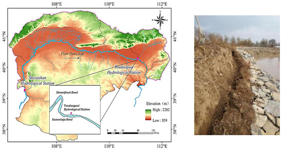
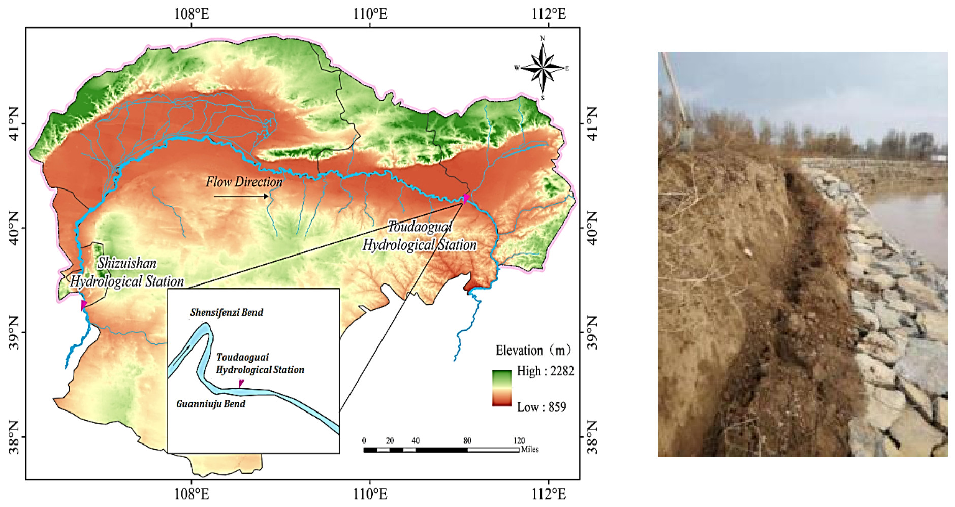
The Shisifenzi Bend, located approximately 4 km upstream of the Toudaoguai Hydrological Station along the Inner Mongolia section of the Yellow River, was selected as the study area. The geographical location of the study area is shown in Figure 1. The channel slope is approximately 0.15‰, with an average river width of about 300 m and an average water depth of approximately 2.85 m [19,20]. The river flows from northeast to southwest, and the bend exhibits an approximately 180° curvature with a curvature coefficient of 3.15. The channel width at the upstream entrance of the bend is approximately 620 m, whereas the downstream exit section narrows substantially to only 215 m, representing a reduction of nearly two-thirds in river width. This region features a typical continental monsoon climate, with a mean annual temperature ranging from 4 °C to 8 °C. The average temperature drops below zero in late November each year, when ice run begins. The river enters the freeze-up stage in early December and breaks up in mid-to-late March of the following year. The ice season generally lasts approximately 130 days, with a maximum duration of 150 days. The maximum historical frozen soil depth is 1.34 m.

Figure 1. Study area location and embankment collapse photo.

The Shisifenzi Bend is a key location for ice-jam-induced river closure along the Inner Mongolia section of the Yellow River. Since 2000, five initial ice-jam events have occurred at this site. Following ice-jam formation, the river water level increases substantially, reaching a maximum elevation of 988.4 m. After river breakup, the minimum water level decreases to 985.5 m, resulting in a water-level difference of 2.9 m during the ice period. The bend exhibits distinct hydraulic characteristics, including deposition along the convex bank and erosion along the concave bank. Therefore, it is considered a critical river reach along the Inner Mongolia section of the Yellow River. Due to ice-period water-level fluctuations and freeze–thaw cycles, instability and collapse frequently occur along the concave bank during the ice-melting period.

2.2. Experimental Design

In accordance with the Standard for Soil Test Methods [21], soil samples were collected from the concave bank of the Shisifenzi Bend. Soil samples were collected vertically at 60 cm intervals, with sampling depths of 0, 60, 120, 180, and 240 cm below the ground surface. Particle size distribution analysis, dry density measurements, and water content measurements were conducted to characterize the basic physical properties of the riverbank soils.

Affected by diurnal temperature difference, variation of freeze–thaw duration and soil temperature gradient, the deterioration rate and magnitude of natural embankment soils exhibit complex variations. To focus on analyzing the effects of water content, dry density and freeze–thaw cycles on soil mechanical properties, and to explore the contribution and influence degree of each factor on soil physico-mechanical properties, uniform and repeatable thermal boundary conditions were adopted in the experiments. Triaxial shear tests were conducted under four water content levels (12.0%, 15.0%, 18.0%, and 21.0%), three confining pressure levels (50, 100, and 150 kPa), and different numbers of freeze–thaw cycles. Based on the recorded minimum winter temperature of −22.6 °C and maximum temperature of 15 °C in recent years [22], the freezing and thawing temperatures were set at −20 °C and 15 °C, respectively. The detailed experimental program is summarized in Table 1.

Table 1. Experimental program for freeze–thaw cycle tests.

Water Content (%)	Confining Pressure (kPa)	Number of Freeze–Thaw Cycles	Freezing/Thawing Temperatures (°C)	Freezing/Thawing Duration (h)
12, 15, 18, 21	50, 100, 150	0, 1, 3, 5, 7, 10	−20 (freezing); 15 (thawing)	12 (freezing); 12 (thawing)

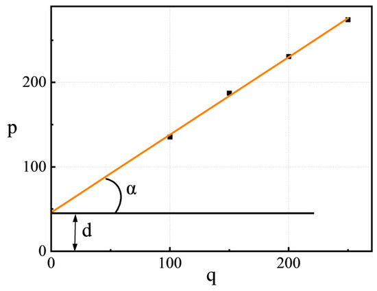
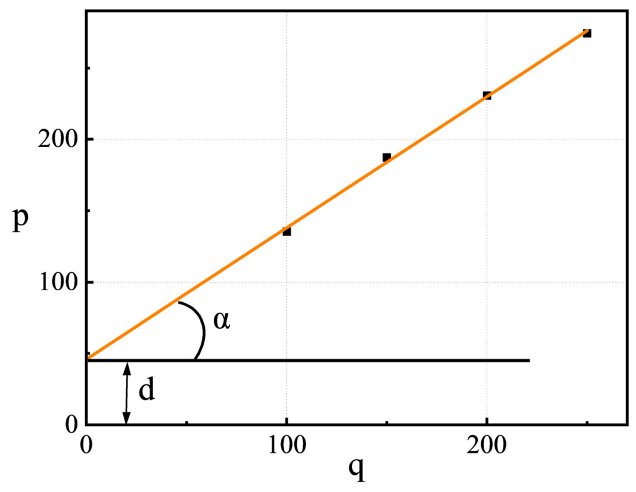
Prior to the freeze–thaw triaxial shear tests, soils with four target water contents were sealed in plastic bags and cured for 24 h to ensure uniform moisture distribution. The required soil masses for triaxial and compression specimens with different initial dry densities and water contents were calculated. The specimens were prepared using a three-piece mold and compacted in five layers. Each layer was scarified before the subsequent layer was compacted to prevent density nonuniformity between layers. Remolded cylindrical triaxial specimens with a height of 80 mm and a diameter of 39.1 mm were obtained. The prepared specimens were subsequently placed in a freeze–thaw chamber for freeze–thaw cycling. Freeze–thaw cycles were performed using a walk-in high–low temperature test chamber (DHT(H)R). Triaxial shear tests were conducted using a strain-controlled triaxial testing apparatus (TSZ10-1.0). The unconsolidated undrained (UU) triaxial shear test was adopted with a strain rate of 0.08 mm/min. Although this test cannot capture the transient pore water pressure and drainage process during soil instability and deformation under multi-factor coupling, it can obtain the macroscopic shear strength parameters of soil under different freeze–thaw cycles, water contents and dry densities, especially the variations in cohesion and internal friction angle. The test was terminated when the axial strain reached 15%, and the maximum deviator stress was adopted as the failure criterion. The failure principal stress lines under different confining pressures were plotted with $p=\left({\sigma }_1-{\sigma }_3\right)/2$ as the vertical axis and $q=\left({\sigma }_1+{\sigma }_3\right)/2$ as the horizontal axis, as shown in Figure 2. The inclination angle of the principal stress line was defined as α, and the intercept on the vertical axis was defined as d. The internal friction angle and cohesion of the soil were determined according to Equations (1) and (2), and the shear strength was subsequently calculated using Equations (3) and (4).

$$\phi ={\sin }^{-1}\left(\tan \alpha \right)$$

(1)

$$c={\displaystyle \frac{d}{\cos \phi }}$$

(2)

$$\tau =c+\sigma \tan \phi$$

(3)

$$\sigma ={\displaystyle \frac{{\sigma }_1+{\sigma }_3}{2}}+{\displaystyle \frac{{\sigma }_1-{\sigma }_3}{2}}\cos 2\left({45}^{\circ }+{\displaystyle \frac{\phi }{2}}\right)$$

(4)

where φ is the internal friction angle of the soil (°); c is the cohesion of the soil (kPa); τ is the shear strength at failure of the soil (kPa); and σ is the normal stress acting on the failure plane of the soil (kPa).

Figure 2. Schematic diagram of principal stress lines at soil failure.

3. Tests Results and Analysis

3.1. Soil Particle Size Distribution

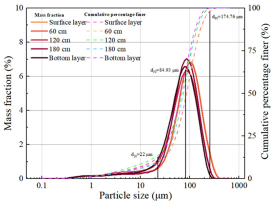
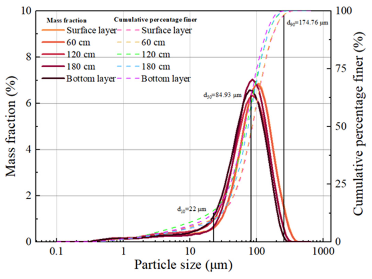
A BT-9300LD laser particle size analyzer (LPSA) was used to characterize the particle size distribution of soil samples. The particle size distribution curves of the surface, middle, and bottom layers are presented in Figure 3. The riverbank soils exhibit evident vertical variations in particle composition. From the surface layer (0–60 cm) to the middle layer (120–180 cm), all soil samples were classified as silty sand (SM). The content of fine particles (<75 μm) exhibited a fluctuating trend with increasing sampling depth, characterized by a slight increase, followed by a rapid increase and subsequent decrease, with corresponding proportions of 35.60%, 36.60%, 47.64%, and 43.87%. The particle size distribution characteristics of the riverbank soils were generally consistent within the study area, although the proportions of different soil fractions varied among sampling depths. Overall, the soils were characterized by high fine particle contents and relatively low coarse particle fractions. Fine components, mainly silt and clay particles, dominated the soil composition. The absence of abrupt changes in the particle size distribution curves suggests relatively uniform particle size characteristics within the study area. Relevant geotechnical tests were carried out to determine key physical parameters of the soil in the study area, including the average water content, dry density, liquid limit and plastic limit, as shown in Table 2.

Figure 3. Soil particle size distribution curve.

Table 2. Physical properties of embankment soils in the study area.

Type	Average Water Content (%)	Average Dry Density (g/cm3)	Liquid Limit (%)	Plastic Limit (%)	Clay Content (%)
Sandy silt	18	1.40	25.7	16.1	14

3.2. Mechanical Properties of Soils

3.2.1. Stress–Strain Behavior of Soils Under Different Water Contents

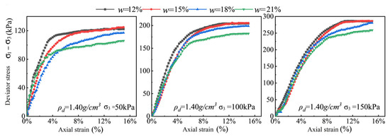
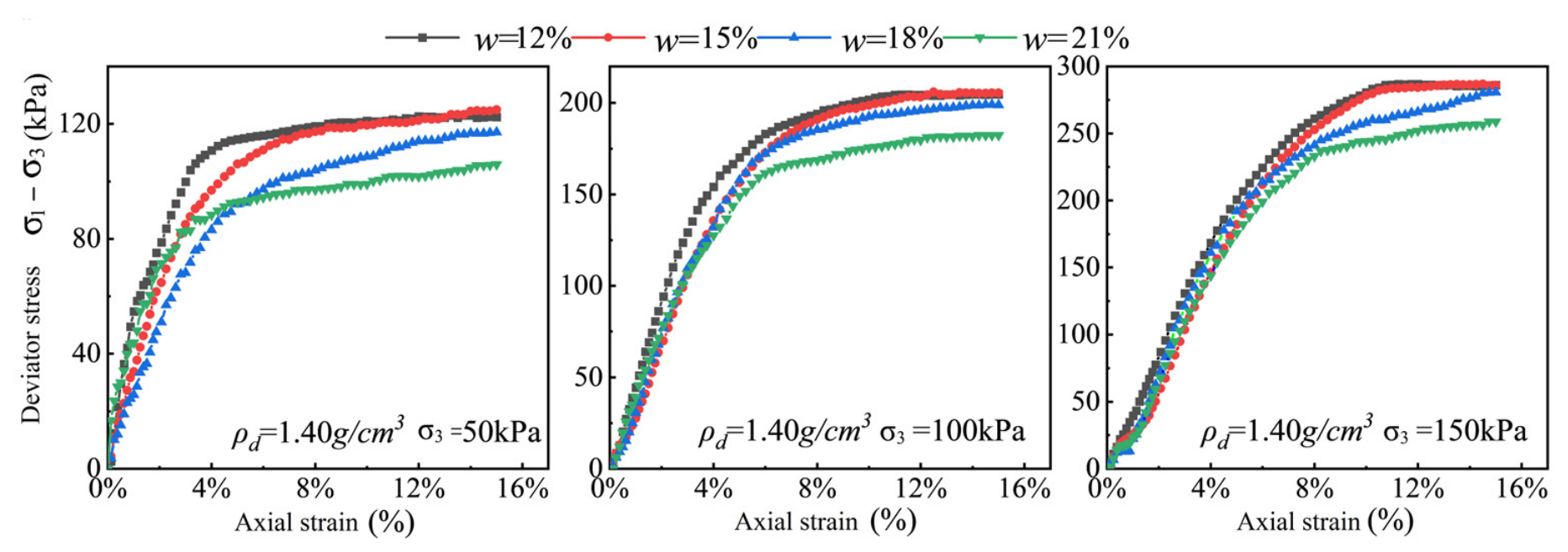
Figure 4 presents the measured shear stress–strain relationships of soils under different confining pressures with varying initial water contents. The results indicate that initial water content has a clear negative relationship with soil shear strength. At all confining pressure levels, the deviator stress of the soil samples exhibited an overall decreasing trend as the initial water content increased from 12% to 21%. Under low water content conditions, the soils exhibited the highest initial tangent modulus and peak strength, accompanied by relatively small axial strains. Subsequently, a certain degree of strain softening was observed after peak strength. As the water content increased to 21%, the peak strength decreased substantially. The stress–strain curves became flatter and smoother, exhibiting more pronounced strain-hardening behavior and ductile failure characteristics. The ultimate strength was also considerably lower than that of specimens with lower water contents. In addition, although increasing confining pressure substantially increased the deviator stress of specimens under all water content conditions by enhancing lateral confinement, it did not alter the fundamental trend of decreasing soil strength with increasing water content.

Figure 4. Stress–strain curves of soil at different initial moisture content.

3.2.2. Evolution of Soil Cohesion

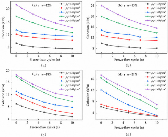
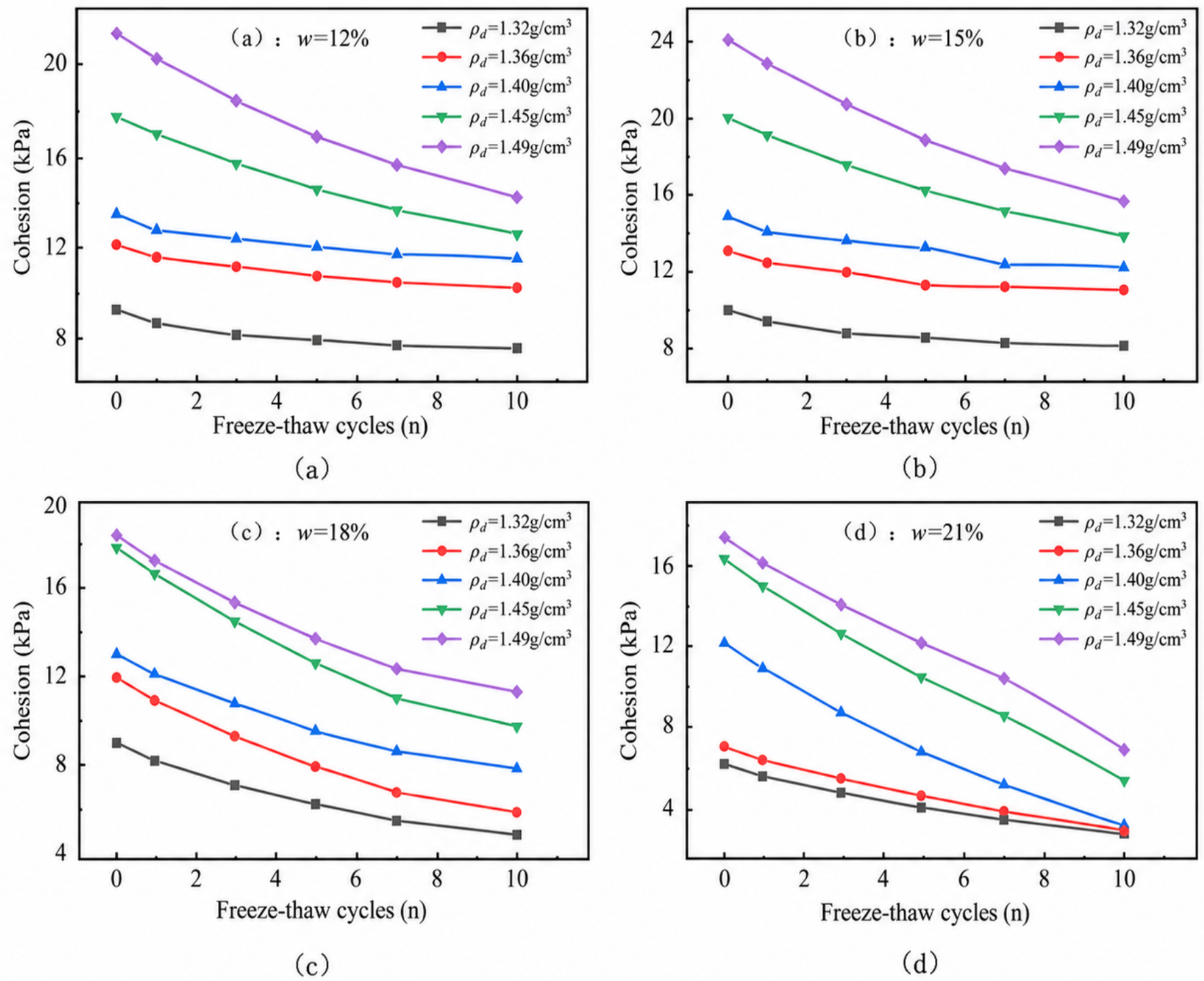
Figure 5 illustrates the evolution of cohesion in riverbank soils with different initial dry densities under four initial water content conditions with increasing numbers of freeze–thaw cycles. Regardless of the combinations of water content and dry density, soil cohesion exhibited a monotonic degradation trend with increasing freeze–thaw cycles, and the degradation process showed distinct stage-dependent characteristics. During the early stage of freeze–thaw cycling (0–3 cycles), the curves exhibited relatively steep declines, indicating that frost heaving pressure caused rapid structural deterioration of the soil. As the number of freeze–thaw cycles increased from 3 to 10, the curves gradually flattened, and the rate of cohesion loss decreased, indicating that the accumulated damage gradually approached stabilization.

Figure 5. Variation in soil cohesion with the number of freeze–thaw cycles, (a) w = 12%; (b) w = 15%; (c) w = 18%; (d) w = 21%.

Initial dry density was the primary factor controlling the absolute level of soil cohesion during freeze–thaw cycling. Under all four water content conditions, the five curves were consistently distributed according to initial dry density, with higher-density soils maintaining substantially higher residual cohesion than lower-density soils after 10 freeze–thaw cycles. Meanwhile, water content affected not only the initial cohesion level but also the freeze–thaw degradation characteristics of soils. At a water content of 15%, soils with different dry densities exhibited the highest initial cohesion. However, when water content increased to 21%, the initial cohesion of soils at all dry density levels decreased substantially. After 10 freeze–thaw cycles, the difference in cohesion among soils with different dry densities became smaller, indicating that high water content weakened the strengthening effect of dry density.

The degradation of cohesion during freeze–thaw cycling is primarily associated with repeated frost-induced stresses generated by pore water phase changes, which disrupt particle bonding and interlocking structures. Soils with higher initial dry density possess smaller void ratios and limited freezable water content, while their denser skeletons provide stronger resistance to frost-induced deformation. In contrast, under high water content conditions, increased pore water content amplifies frost-induced stresses and weakens particle bonding, leading to irreversible structural loosening and cohesion loss during freeze–thaw cycles.

3.2.3. Evolution of Soil Internal Friction Angle

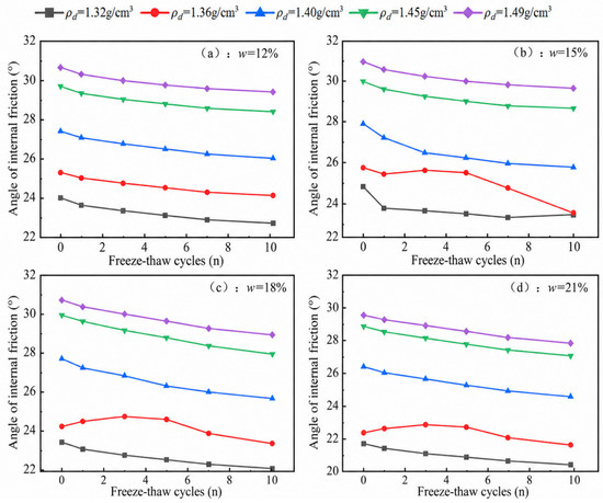
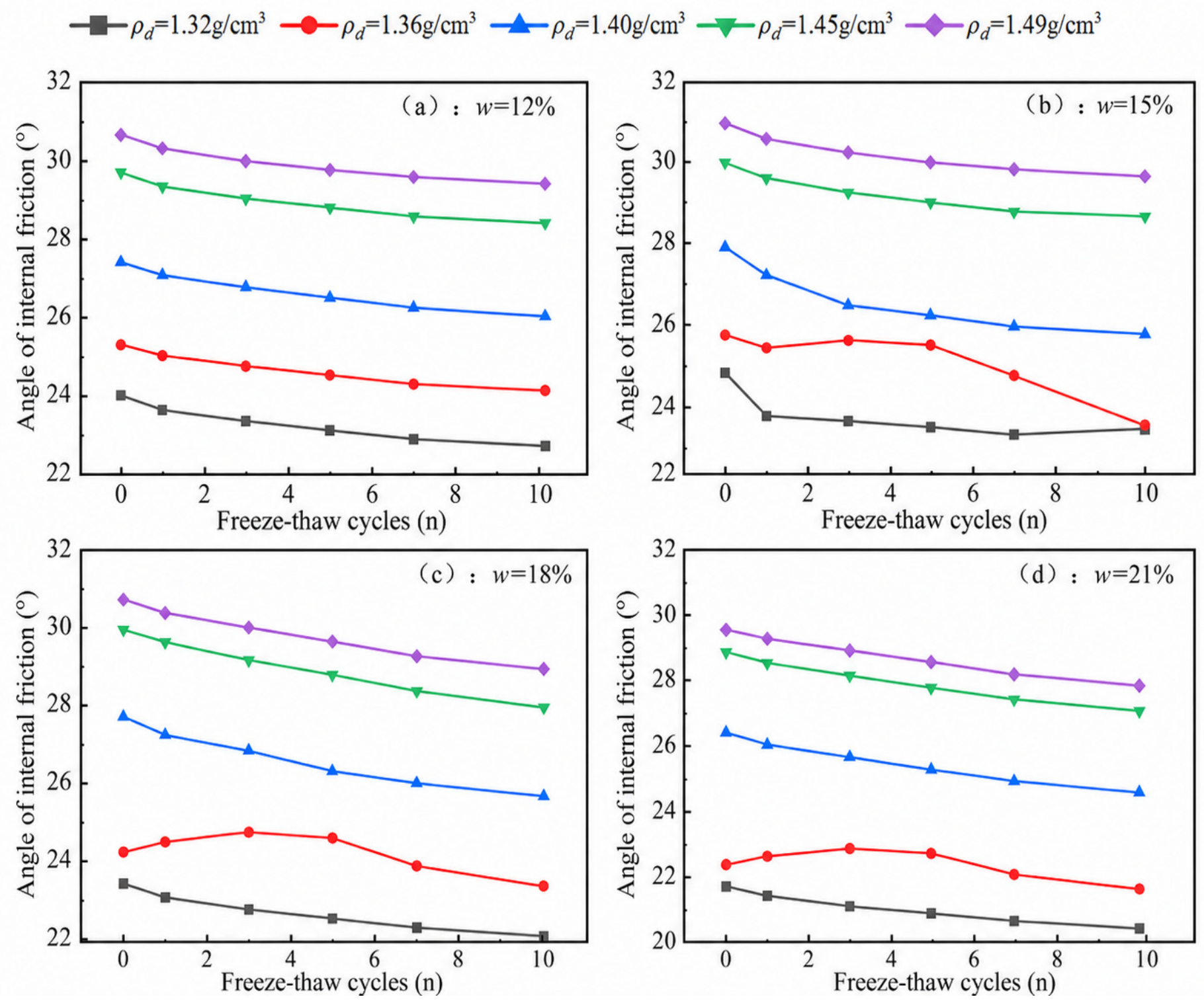
Figure 6 presents the variations in the internal friction angle of riverbank soils with freeze–thaw cycles and initial dry density under different initial water contents. Under different water contents, initial dry density consistently dominated the absolute level of internal friction angle. In all panels, the five curves exhibited a clear vertical arrangement according to initial dry density, with denser soils maintaining higher internal friction angles throughout the 10 freeze–thaw cycles. As shown in Figure 6a, regarding the effect of freeze–thaw cycling, the internal friction angle of soils at different dry densities generally exhibited a slight decreasing trend with increasing freeze–thaw cycles. However, Figure 6b,c, shows that the internal friction angle of soils with low initial dry density remained stable or even slightly increased locally during the early freeze–thaw stage (0–3 cycles). This phenomenon may be attributed to the temporary enhancement of particle interlocking in loose soils caused by ice crystal compression during the initial freeze–thaw stage. However, with continued cycling, the degradation rate increased, indicating the irreversible accumulation of freeze–thaw damage. Meanwhile, water content had a considerable influence on the internal friction angle. Within the water content range of 15–18%, soils with different dry densities exhibited relatively high initial internal friction angles, which was consistent with the existence of an optimum water content (approximately 15%) for the tested soils. When the water content increased to 21%, the overall internal friction angle decreased substantially, and high-density soils (e.g., 1.49 g/cm³) also exhibited greater strength losses under freeze–thaw conditions, as shown in Figure 6d.

Figure 6. Variation of internal friction angle with the number of freeze–thaw cycles, (a) w = 12%; (b) w = 15%; (c) w = 18%; (d) w = 21%.

3.3. Sensitivity Analysis of Factors Influencing Soil Shear Strength

To quantitatively determine the relative importance of initial dry density, water content, and freeze–thaw cycles on soil shear strength, analysis of variance (ANOVA) was employed to evaluate the statistical significance of these key influencing factors. The effects of initial dry density, water content, and freeze–thaw cycle number on soil shear strength parameters were systematically examined, providing statistical evidence for understanding the mechanical evolution of riverbank soils under multi-field coupling conditions.

Considering the potential interactions among different factors, a statistical model containing second-order interaction terms was established:

$$Y=\mu +A_w+B_{\rho }+C_N+A_w{B}_{\rho }+A_w{C}_N+B_{\rho }{C}_N+\epsilon$$

(5)

where Y represents the soil shear strength parameters, including cohesion and internal friction angle under different normal stress conditions. A_w, $B_{\rho }$, and C_N represent the effects of water content, dry density, and freeze–thaw cycle number, respectively. A_w$B_{\rho }$, A_wC_N, and B_ρC_N denote the interaction effects between water content and dry density, water content and freeze–thaw cycles, and dry density and freeze–thaw cycles, respectively. ε represents the random error.

Four water contents, five dry densities, and six freeze–thaw cycle levels were considered in this experiment, resulting in a total of 120 test combinations. The effects of different factors on soil shear strength were evaluated using the sum of squares (SS), mean square (MS), F-statistic, and significance level (p-value). In addition, the contribution ratio was used to quantify the contribution of each factor to the total variation. The contribution rate is calculated as the ratio of the sum of squares of each factor to the total sum of squares. It is used to quantify the relative contribution of different factors to the total variation of the response variable, and its calculation formula is:

$${\eta }_i={\displaystyle \frac{S{S}_i}{S{S}_T}}\times 100\%$$

(6)

where η_i represents the contribution ratio of the ith influencing factor, SS_i is the corresponding sum of squares of the ith factor, and SS_T represents the total sum of squares.

To verify the accuracy of the multi-factor analysis of variance (ANOVA) model with multiple interaction terms, the coefficient of determination $R^2$ and adjusted coefficient of determination $R_{adj}^2$ are introduced. Their formulas are given below:

$$R^2={\displaystyle \frac{S{S}_M}{S{S}_T}}={\displaystyle \frac{S{S}_T-S{S}_E}{S{S}_T}}$$

(7)

$$R_{adj}^2=1-{\displaystyle \frac{S{S}_E/d{f}_E}{S{S}_T/d{f}_T}}$$

(8)

where ${SS}_M$ is the model sum of squares, ${SS}_E$ is the error sum of squares, ${df}_E$ denotes the degrees of freedom for error, and ${df}_T$ denotes the total degrees of freedom.

Table 3 presents the ANOVA results for cohesion. The results indicate that dry density was the dominant factor affecting cohesion, with a contribution ratio of 60.199%. Increasing dry density enlarged the contact area among soil particles and enhanced particle bonding, thereby improving soil structural stability. Water content was the second most influential factor, with a contribution ratio of 19.618%. Variations in water content altered the pore conditions between soil particles. During freeze expansion and thaw contraction processes, changes in water content weakened particle interlocking, thereby affecting soil cohesion. Freeze–thaw cycle number also exhibited a considerable influence on cohesion, with a contribution ratio of 15.940%. This effect was mainly attributed to the repeated destruction of internal bonding structures caused by freeze–thaw processes, resulting in cohesion degradation. Furthermore, the three interaction terms accounted for 4.244% of the total contribution, indicating that interactions among water content, dry density, and freeze–thaw cycles also influenced the cohesive structure of the soil.

Table 3. ANOVA results for cohesion c.

Factor	Sum of Squares (SS)	Degree of Freedom (df)	Mean Square (MS)	F-Value	p-Value	Contribution Ratio (%)
Water content, w	454.92	3	151.64	501.30	<0.001	19.618
$\mathrm{Dry}\mathrm{density},{\rho }_d$	1395.95	4	349.00	1153.72	<0.001	60.199
$\mathrm{Freeze}–\mathrm{thaw}\mathrm{cycles},n$	369.64	5	73.93	244.40	<0.001	15.940
$w\times {\rho }_d$	24.02	12	2.00	6.62	<0.001	1.036
$w\times n$	19.87	15	1.33	4.38	<0.001	0.857
${\rho }_d\times n$	54.51	20	2.73	9.01	<0.001	2.351
Error	18.15	60	0.30	—	—	0.783

Table 4 presents the ANOVA results for the internal friction angle $\phi$. Similar to cohesion, the internal friction angle was predominantly controlled by dry density, which accounted for 88.556% of the total contribution, far exceeding the contributions of water content and freeze–thaw cycles. This is because the internal friction angle primarily reflects friction and interlocking among soil particles, whereas changes in dry density directly modify particle arrangement and interparticle contact conditions. The contribution of freeze–thaw cycles to the internal friction angle was relatively small, at only 3.215%, consistent with the experimental observations. This suggests that freeze–thaw action primarily affects the structural integrity of the soil, while its influence on interparticle friction is comparatively limited.

Table 4. ANOVA results for internal friction angle φ.

Factor	Sum of Squares (SS)	Degree of Freedom (df)	Mean Square (MS)	F-Value	p-Value	Contribution Ratio (%)
$\mathrm{Water}\mathrm{content},w$	64.11	3	21.37	736.27	<0.001	7.062
$\mathrm{Dry}\mathrm{density},{\rho }_d$	803.96	4	200.99	6924.54	<0.001	88.55
$\mathrm{Freeze}–\mathrm{thaw}\mathrm{cycles},n$	29.19	5	5.84	201.13	<0.001	3.215
$w\times {\rho }_d$	7.49	12	0.62	21.49	<0.001	0.825
$w\times n$	0.52	15	1.33	1.18	<0.001	0.057
${\rho }_d\times n$	2.59	20	2.73	4.464	<0.001	0.285
Error	1.74	60	0.30	—	—	0.192

The coefficient of determination $R^2=0.992$ and adjusted coefficient of determination $R_{adj}^2=0.985$ for the cohesion model, together with $R^2=0.998$ and $R_{adj}^2=0.986$ for the internal friction angle model, were calculated from the ANOVA sum of squares. $R^2$ is slightly higher than $R_{adj}^2$, yet no marked reduction is observed after adjustment, which indicates that the interaction terms included in the model are statistically significant. The adjusted coefficients of determination for both cohesion and internal friction angle are close to 1, demonstrating that the ANOVA model with main effects and second-order interaction effects possesses strong explanatory power for the experimental results. Water content, dry density, freeze–thaw cycle number and their coupled interactive effects can account for most of the variation in soil shear strength parameters. The small p-values are now reported as evidence that the corresponding effects are statistically detectable within the tested factorial design. Practical importance is instead discussed together with effect magnitude and the contribution ratio. This also suggests low random error and high reliability of the experimental data in this study.

The factors affecting soil cohesion and internal friction angle are ranked as dry density, water content and freeze–thaw cycle number. Among them, dry density is the dominant factor governing shear strength, while freeze–thaw cycles exert a vital effect on cohesion degradation by disrupting the cemented structure of soil. The shear performance of freeze–thawed soil is jointly controlled by three mechanisms: dry density determines the initial strength level, water content modulates the magnitude of freeze–thaw damage, and freeze-thaw cycles accelerate structural deterioration.

Overall, the three-factor ANOVA results indicate that dry density, water content, and freeze–thaw cycle number ranked in descending order of influence on both cohesion and internal friction angle. Dry density was the dominant factor controlling the initial level of soil shear strength, whereas freeze–thaw cycling played an important role in cohesion degradation by progressively disrupting the internal bonding structure of the soil. The shear behavior of freeze–thaw-affected soils therefore reflects the combined effects of three processes: dry density governs the initial strength level, water content regulates the extent of freeze–thaw-induced deterioration, and repeated freeze–thaw cycles promote progressive structural degradation.

4. Development and Application of a Thermo-Hydro-Mechanical Coupled Model for Riverbank Stability

4.1. Governing Equations

4.1.1. Governing Equation for the Temperature Field

Based on the principle of energy conservation, the net heat inflow into an infinitesimal soil element per unit time is equal to the rate of increase in its internal energy plus the internal heat-source term. Accordingly, the heat-conduction equation for frozen soil, accounting for the latent heat associated with ice–water phase change, can be expressed as:

$$\lambda {\nabla }^{2}T\cdot dxdydzdt+L{\rho }_i{\displaystyle \frac{\partial {\theta }_i}{\partial t}}dt\cdot dxdydz=\rho C\left(\theta \right){\displaystyle \frac{\partial T}{\partial t}}dt\cdot dxdydz$$

(9)

where $\lambda$ is the effective thermal conductivity of the soil (W·m⁻¹K⁻¹); $\rho$ is the dry density of the soil (kg·m⁻³); $T$ is the temperature (°C); $t$ is time (s); ${\rho }_i$ is the density of ice (kg·m⁻³); $L$ is the latent heat of phase change, taken as $3.34\times {10}^5$ J·kg⁻¹; $\theta$ is the porosity, with $\theta ={\theta }_w+{\theta }_i$, where ${\theta }_w$ and ${\theta }_i$ are the volumetric contents of unfrozen water and ice, respectively (m³·m⁻³); and $C\left(\theta \right)$ is the specific heat capacity of the soil (J·kg⁻¹K⁻¹).

Equation (9) can be simplified to obtain the governing equation for the temperature field of frozen soil [23]:

$$C_v{\displaystyle \frac{\partial T}{\partial t}}=\lambda \left(\theta \right){\nabla }^{2}T+L{\rho }_i{\displaystyle \frac{\partial {\theta }_i}{\partial t}}$$

(10)

where C_v = ρC(θ) is the volumetric heat capacity of the soil (J·m⁻³K⁻¹).

4.1.2. Governing Equation for the Moisture Field

According to the law of mass conservation and Darcy’s law for unsaturated soils, the change in the mass of liquid water within an infinitesimal element of frozen soil per unit time is equal to the sum of the net inflow of liquid water and the mass change induced by the ice–water phase transition. The flow of liquid water is driven by the gradient of the total hydraulic head. Accordingly, the governing equation for moisture migration during freeze–thaw processes can be expressed as [24]:

$${\displaystyle \frac{\partial {\theta }_w}{\partial t}}+{\displaystyle \frac{{\rho }_i}{{\rho }_w}}{\displaystyle \frac{\partial \theta i}{{\partial }_t}}=\nabla [D(\theta )\nabla {\theta }_w+K({\theta }_w)]$$

(11)

where ${\rho }_w$ is the density of water (kg·m⁻³); $K\left({\theta }_w\right)$ is the unsaturated hydraulic conductivity; and $D\left(\theta \right)$ is the moisture diffusivity. The unsaturated hydraulic conductivity $K\left({\theta }_w\right)$ and moisture diffusivity $D\left(\theta \right)$ of frozen soil can be calculated as follows:

$$D\left({\theta }_w\right)={\displaystyle \frac{K\left({\theta }_w\right)}{c\left({\theta }_w\right)}}\cdot I$$

(12)

$$K\left({\theta }_w\right)=k_s{S}^l{\left[1-{\left(1-S^{1/m}\right)}^m\right]}^2$$

(13)

$$c\left({\theta }_w\right)={\displaystyle \frac{1}{a}}{\left(S^{-1/m}-1\right)}^{1-m}$$

(14)

where $k_s$ is the saturated hydraulic conductivity (m·d⁻¹); $l$ is the pore-connectivity parameter, commonly taken as 0.5; and $m$ is an empirical parameter related to the pore-size distribution. Here, $c\left({\theta }_w\right)$ is the specific moisture capacity (m⁻¹), and $I$ is the impedance factor representing the inhibitory effect of ice content on moisture migration. The impedance factor is calculated as [25]:

$$I={10}^{-10{\theta }_i}$$

(15)

4.1.3. Governing Equation for the Stress Field

Under freeze–thaw conditions, the total strain of the soil consists of the elastic strain induced by external loading and the volumetric strain induced by moisture phase change and migration [26], expressed as:

$$\epsilon ={\epsilon }_{ij}^e+{\epsilon }_{ij}^v$$

(16)

where ${\epsilon }_{ij}^e$ represents the elastic strain induced by external loading, and ${\epsilon }_{ij}^v$ represents the volumetric strain induced by moisture phase change and migration. The strain associated with moisture phase change and migration can be calculated as:

$${\epsilon }_{ij}^v=0.09\left({\theta }_o+{\Delta }_{\theta }-{\theta }_u\right)+\Delta \theta +\left({\theta }_o-n\right)$$

(17)

The model proposed in this paper is mainly used to investigate the macroscopic evolution of temperature field, moisture field, displacement field and embankment slope stability, rather than to precisely describe the complex plastic behavior of soil during freeze–thaw cycles. Therefore, the constitutive equation adopts a linear elastic constitutive relation considering initial strain. Combined with the Mohr-Coulomb strength criterion, the soil constitutive equations are expressed as:

$$\left\{\sigma \right\}=\left[C\right]\left(\left\{\epsilon \right\}-\left\{{\epsilon }_0\right\}\right)$$

(18)

$$\tau =c+\sigma \tan \phi$$

(19)

where $\left\{\sigma \right\}$ is the stress vector; $\left[C\right]$ is the material stiffness matrix; $\left\{\epsilon \right\}$ is the total strain vector; and $\left\{{\epsilon }_0\right\}$ is the initial strain vector. In Equation (19), $c$ is the soil cohesion, $\phi$ is the internal friction angle, $\sigma$ is the normal stress, and $\tau$ is the shear stress. By combining the above governing equations with the constitutive relations and discretizing the system using the finite element method (FEM), the displacement field, stress field, and distribution of plastic zones within the bank slope can be obtained.

4.1.4. Coupling Theory for the Moisture and Temperature Fields

During soil freezing, moisture migration and temperature distribution are strongly coupled through bidirectional interactions. On the one hand, the temperature gradient not only indirectly affects matric potential and moisture transport parameters by altering the viscosity and surface tension of water, but can also directly drive moisture migration. On the other hand, the latent heat associated with moisture phase change and variations in water content significantly affect the temperature distribution. To enable the coupled solution of the temperature and moisture fields, the ratio of the volumetric ice content to the volumetric unfrozen water content, $B_i$, is introduced as the key coupling variable, thereby linking the dependent variables of the two fields through the phase equilibrium relationship. The resulting hydrothermal coupling relationship is expressed as [27,28]:

$$B_i={\displaystyle \frac{{\theta }_i}{{\theta }_u}}\left\{\begin{array}{c}\begin{array}{cc}1.1{\left({\displaystyle \frac{T}{T_f}}\right)}^b-1,& T<T_f\end{array}\\ \begin{array}{ccc}0,& & T\ge T_f\end{array}\end{array}\right.$$

(20)

where $T_f$ is the soil freezing temperature (°C), and $b$ is a constant that varies with soil type and salt content, with values of 0.61 for sandy soil, 0.47 for silty soil, and 0.56 for clayey soil.

Based on the temperature-field and moisture-field formulations described above, the coupled hydrothermal governing equations for frozen soil can be expressed as:

$$\theta ={\theta }_w+{\displaystyle \frac{{\rho }_i}{{\rho }_w}}{\theta }_i$$

(21)

$$B_i={\displaystyle \frac{{\theta }_i}{{\theta }_w}}=f\left(T\right)$$

(22)

The above system of equations couples the temperature and moisture fields through the dynamic evolution of unfrozen water and ice contents, thereby describing the coupled evolution of moisture migration, latent heat associated with phase change, and temperature distribution during freeze–thaw processes. By explicitly incorporating the water–ice phase-transition relationship and the latent-heat term, bidirectional feedback between the two fields is represented.

4.2. Geometric Model Development and Validation

4.2.1. Model Development

COMSOL6.4 Multiphysics was employed for the numerical simulations. The temperature and moisture fields were implemented using the Coefficient Form PDE interface, whereas the displacement field was modeled using the built-in Solid Mechanics interface. In this way, a fully coupled thermo-hydro-mechanical (THM) model was established.

The general form of the coefficient-form partial differential equation in COMSOL Multiphysics is expressed as [29]:

$$e_a{\displaystyle \frac{{\partial }^{2}u}{\partial t^2}}+d_a{\displaystyle \frac{\partial u}{\partial t}}+\nabla \left(-c\nabla u-\alpha u+\gamma \right)+\beta \cdot \nabla u+au=f$$

(23)

where $e_a$ is the mass coefficient (s²); $d_a$ is the damping coefficient [J·m⁻³·K⁻¹]; $c$ is the diffusion coefficient [W·m⁻¹·K⁻¹]; $\alpha$ is the conservative-flux convection coefficient (m⁻¹); $\gamma$ is the conservative-flux source term (W·m⁻²); $\beta$ is the convection coefficient [W·m⁻²·K⁻¹]; $a$ is the absorption coefficient [W·m⁻³·K⁻¹]; and $f$ is the source term (W·m⁻³).

The governing equation for the temperature field was then combined with the hydrothermal coupling relationship, yielding:

$$\rho C\left(\theta \right){\displaystyle \frac{\partial T}{\partial t}}=\lambda \left(\theta \right){\nabla }^{2}T+L{\rho }_i\left({\theta }_s-{\theta }_r\right)\left[S{\displaystyle \frac{\partial B_i}{\partial t}}+B_i{\displaystyle \frac{\partial S}{\partial t}}\right]+L{\rho }_i{\theta }_r{\displaystyle \frac{\partial B_i}{\partial t}}$$

(24)

Rearranging Equation (24) into the coefficient form required by the PDE interface gives:

$$\left\{\begin{array}{c}{d}_a=\rho C-L{\rho }_i\left[\left({\theta }_s-{\theta }_r\right)S+{\theta }_r\right]{\displaystyle \frac{\partial B\left(T\right)}{\partial T}}\\ c=\lambda \left(\theta \right)\\ f=L{\rho }_i\left({\theta }_s-{\theta }_r\right)B\left(T\right){\displaystyle \frac{\partial S}{\partial t}}\end{array}\right.$$

(25)

Because the remaining terms in the general coefficient-form equation have no corresponding terms in the temperature-field governing equation, the coefficients $a$, $\gamma$, $\beta$, $\alpha$, and $e_a$ were all set to zero.

Similarly, the coefficient inputs for the moisture field were obtained as:

$$\left\{\begin{array}{c}{d}_a=1+B_i{\displaystyle \frac{{\rho }_i}{{\rho }_w}}\\ c=D\left(S\right)\\ \gamma =-K\left(S\right)\\ a={\displaystyle \frac{{\rho }_i}{{\rho }_w}}{\displaystyle \frac{\partial B_i}{{\partial }_t}}\\ f={\displaystyle \frac{{\rho }_i}{{\rho }_w}}{\displaystyle \frac{{\theta }_r}{{\theta }_s-{\theta }_r}}{\displaystyle \frac{\partial B_i}{{\partial }_t}}\end{array}\right.$$

(26)

For the moisture-field equation, $e_a$, $\alpha$, and $\beta$ in the general coefficient-form equation were set to zero.

For the simulation of frost-heave deformation, the Thermal Expansion feature in the Solid Mechanics interface was used to represent changes in ice volume as an equivalent thermal strain. Since the triaxial tests in this paper are mainly conducted to obtain shear strength parameters under different freeze–thaw conditions, and the critical ice content at the initiation of frost heave was not specifically measured, research results for loam are referenced, and this parameter is assigned a value of 2.7% [30]. The uncertainty in the critical ice content for frost-heave initiation may affect the simulation accuracy of frost-heave displacement in the early freezing stage, leading to relatively large displacement errors of the model at the onset of freezing.

The relationship between the frost-heave coefficient and ice content was defined as:

$$\eta \left(x,y\right)=\left\{\begin{array}{ll}0.0156{\omega }_{\theta i}-0.0042,& {\omega }_{\theta i}>0.027\\ 0,& {\omega }_{\theta i}<0.027\end{array}\left(loam\right)\right.$$

(27)

where $w_{\theta i}$ is the mass fraction corresponding to the ice content ${\theta }_i$, calculated as:

$${\omega }_{\theta i}={\displaystyle \frac{{\rho }_i}{{\rho }_{\omega }}}\cdot {\displaystyle \frac{{\theta }_i}{{\rho }_s}}$$

(28)

4.2.2. Model Validation

To accurately simulate temperature field evolution, moisture migration and accumulation, and frost-heave deformation caused by ice–water phase change of soil during freezing in seasonally frozen regions, the reliability and computational accuracy of the developed thermo-hydro-mechanical (THM) multi-field coupled model need to be validated. Owing to the absence of continuous field measurements of ground temperature, water content, pore pressure and deformation for the target slope, field validation on the real riverbank cannot be carried out. Hence, the well-known laboratory one-dimensional freezing soil column test reported by Lu Song is chosen to separately verify the hydrothermal coupling and solid mechanics modules of the model, so as to demonstrate the validity of the physical mechanisms and numerical approaches adopted.

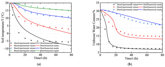
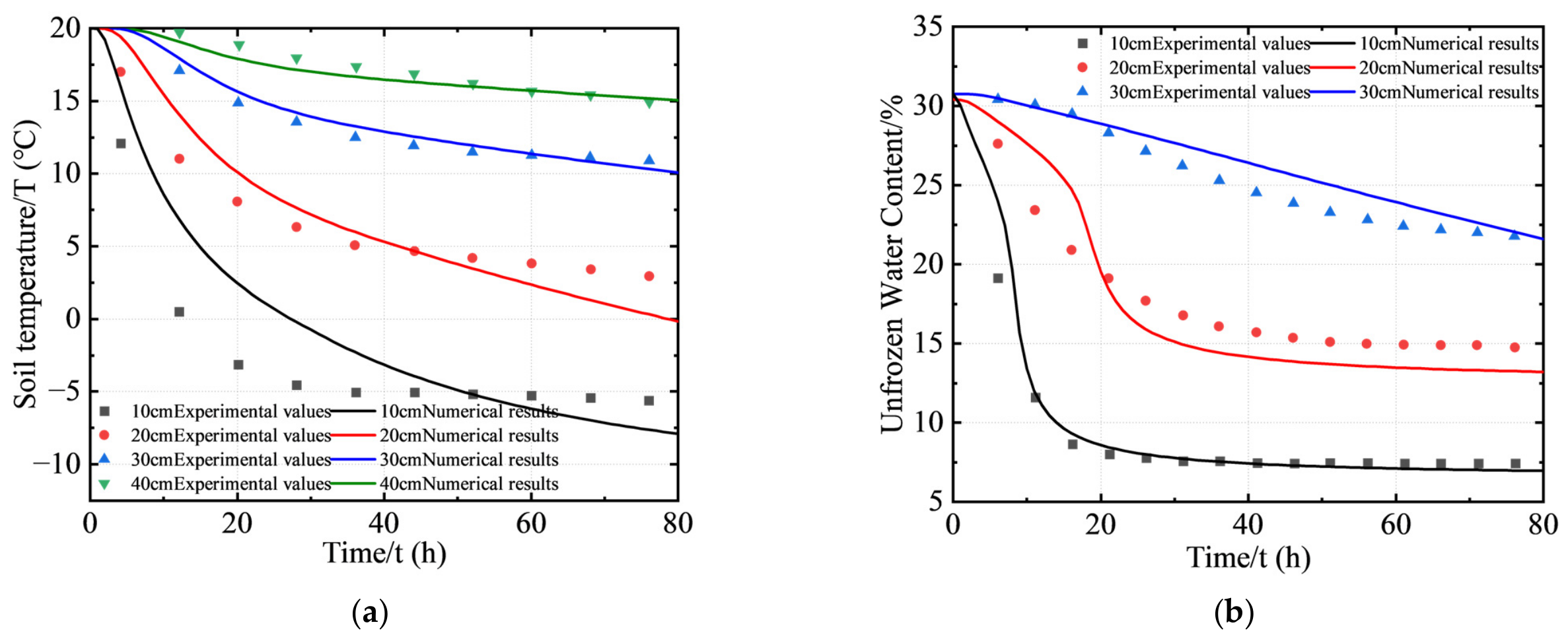
In the closed-system one-dimensional freezing soil-column experiment, monitoring points were arranged at depths of 10, 20, 30, and 40 cm below the top of the soil column, and temporal variations in temperature and water content were recorded at each depth [31]. Figure 7 compares the simulated and measured temperature and water-content values at different depths and freezing times. Overall, the simulated results reproduced the measured trends well at all four monitoring depths throughout the 0–80 h freezing period.

Figure 7. Comparison of experimental and simulation results: (a) temperature field, (b) moisture content.

During the initial stage of freezing, the simulated rate of temperature decrease agreed well with the experimental observations, and the temperature curves were nearly coincident. The maximum absolute temperature error was less than 2 °C, with the relative error remaining within 8% over the corresponding range. For water content, the maximum absolute error was less than 3%, and the relative error remained within 10%. As the freezing front migrated downward, pronounced moisture migration and accumulation occurred near the freezing interface. At this stage, the mean absolute temperature error at each monitoring depth remained below 3 °C, while the relative error over the full range was within 12%.

As the phase-transition process approached completion, the rate of decrease in unfrozen water content gradually slowed and tended toward a stable state. The mean absolute error in unfrozen water content at each depth was less than 4%. A slightly larger deviation occurred at the shallow 10 cm monitoring point during the later stage, mainly because of the stronger influence of boundary heat exchange. Overall, the relative error of the hydrothermal model over the entire freezing period was within 12% for temperature and within 15% for unfrozen water content, while the relative errors during the active phase-transition stage were both maintained within 10%.

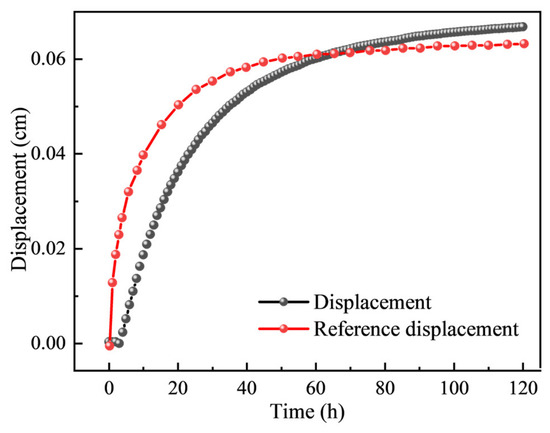
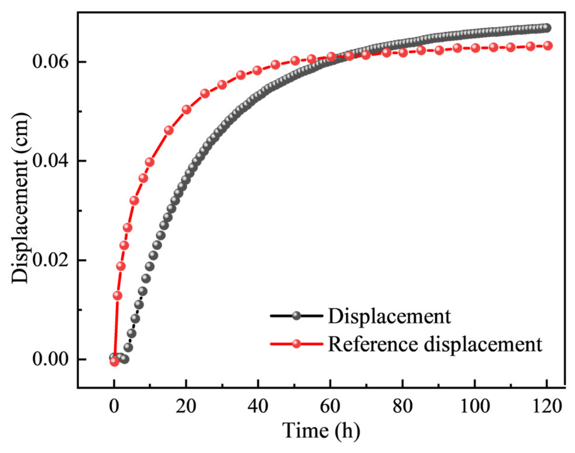
Figure 8 compares the measured and simulated displacement at the top of the soil column over time. Overall, the simulated and measured curves exhibited consistent temporal trends, both showing a distinct three-stage evolution characterized by rapid initial growth, a subsequent reduction in growth rate, and eventual stabilization. During the initial stage (0–60 h), both curves increased steeply, corresponding to the period of the most rapid frost-heave development over the entire freezing process. The simulated displacement was generally slightly lower than the measured value during this stage, with a maximum absolute error of approximately 0.014 cm and a corresponding relative error of approximately 28%. The main reason is that the ice–water phase change, moisture migration and frost-heave process are intense at the initial freezing stage. The model proposed in this paper simplifies the phase equilibrium and frost-heave relationship, which leads to certain deviations between the simulated displacements and measured values. As the freezing process proceeds, the error between the simulated and measured results gradually decreases. The two curves intersected at approximately 60 h. During the subsequent stage from 60 to 120 h, the displacement growth rates decreased simultaneously and gradually approached a stable state. The simulated values became slightly higher than the measured values, and the deviation increased slowly with time. At 120 h, the final absolute error was approximately 0.004 cm, corresponding to a relative error of approximately 6.3%. Throughout the freezing process, the simulated and measured displacements exhibited consistent evolutionary behavior and generally good agreement. This indicates that the model can reasonably reproduce the overall evolution trend and the later stable characteristics of frost-heave deformation, whereas the quantitative prediction accuracy for the rapid frost-heave deformation in the initial freezing stage still needs to be improved.

Figure 8. Comparison of displacement versus time between experimental and model results.

4.3. Simulation Results and Analysis for the Typical Cross-Section

4.3.1. Geometric Model and Mesh Discretization

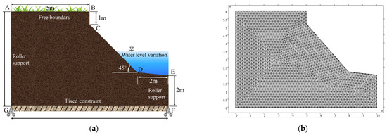
To analyze the evolution of internal stress–strain, displacement and bank slope stability of the embankment within a complete freeze–thaw cycle, a typical bank slope cross-section of the Yellow River (Inner Mongolia Reach) is selected for simulation and analysis. Figure 9a shows the selected typical cross-section of the riverbank at the Shisifenzi Bend along the Inner Mongolia reach of the Yellow River. The riverbank is approximately 6 m high. The middle portion of the bank slope consists of an inclined section with a slope angle of approximately 45°, while the bank toe comprises a 2 m-high vertical bank face and a 0.2 m-high stepped gentle-slope transition section.

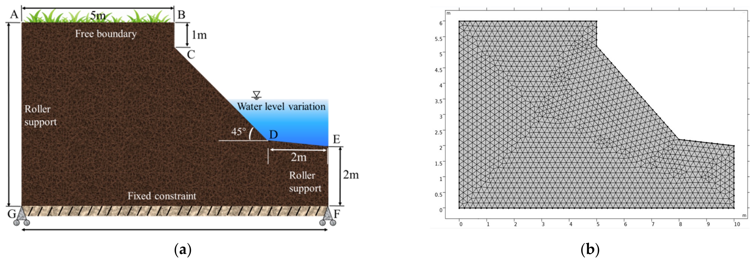
Figure 9. Construction of the geometric model and mesh generation for a typical embankment: (a) geometric model; (b) mesh generation.

The computational domain was discretized using an unstructured triangular mesh, as shown in Figure 9b. The maximum and minimum element sizes were set to 0.2 m and $7.5\times {10}^{-4}$m, respectively, resulting in a total of 2941 mesh elements.

For temporal discretization, the time step was set to 1 day over the complete 130-day freeze–thaw period. The temperature field, moisture field, and Solid Mechanics field were incorporated into a unified transient solution framework. Through temporal discretization, the continuous transient process was divided into 130 discrete time steps, at which the coupled multiphysics equations were solved simultaneously. This scheme enabled the coupled freeze–thaw simulation to proceed on a daily basis from the prescribed initial conditions throughout the entire freeze–thaw period.

4.3.2. Boundary Conditions

A time-dependent surface temperature boundary was prescribed for the temperature field to reproduce the environmental temperature variation over a complete 130-day freeze–thaw period in the study area. The air temperature along the riverbank generally exhibits a sinusoidal seasonal variation. The daily mean temperature falls below 0 °C in November and decreases progressively to its minimum in late January, with a mean January temperature of approximately −15 °C. It then gradually rises and exceeds 0 °C around early April, corresponding to a complete freeze–thaw period of approximately 130 days.

For the moisture field, a closed-system boundary condition was adopted, with no external water supply or drainage considered. The analysis therefore focused on moisture migration and redistribution within the bank slope driven by temperature gradients and gravity. Zero-flux conditions were imposed on the top, bottom, and lateral boundaries to ensure conservation of water within the system. This configuration was used to isolate the dominant sequence of moisture redistribution during freezing and thawing, including temperature-gradient-driven migration toward the freezing front, moisture accumulation near the freezing front, and subsequent redistribution toward deeper soil layers during thawing.

For the mechanical field, the bottom boundary was fixed to constrain both vertical and horizontal displacements, while roller constraints were applied to the two lateral boundaries to restrict only the normal displacement. The slope surface was treated as a free boundary [32]. This combination of mechanical boundary conditions allows the deformation response of the bank slope under the combined effects of self-weight and freeze–thaw action to be represented while minimizing artificial disturbance of the internal stress–strain evolution caused by boundary constraints.

4.3.3. Simulation Results and Analysis

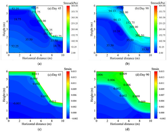
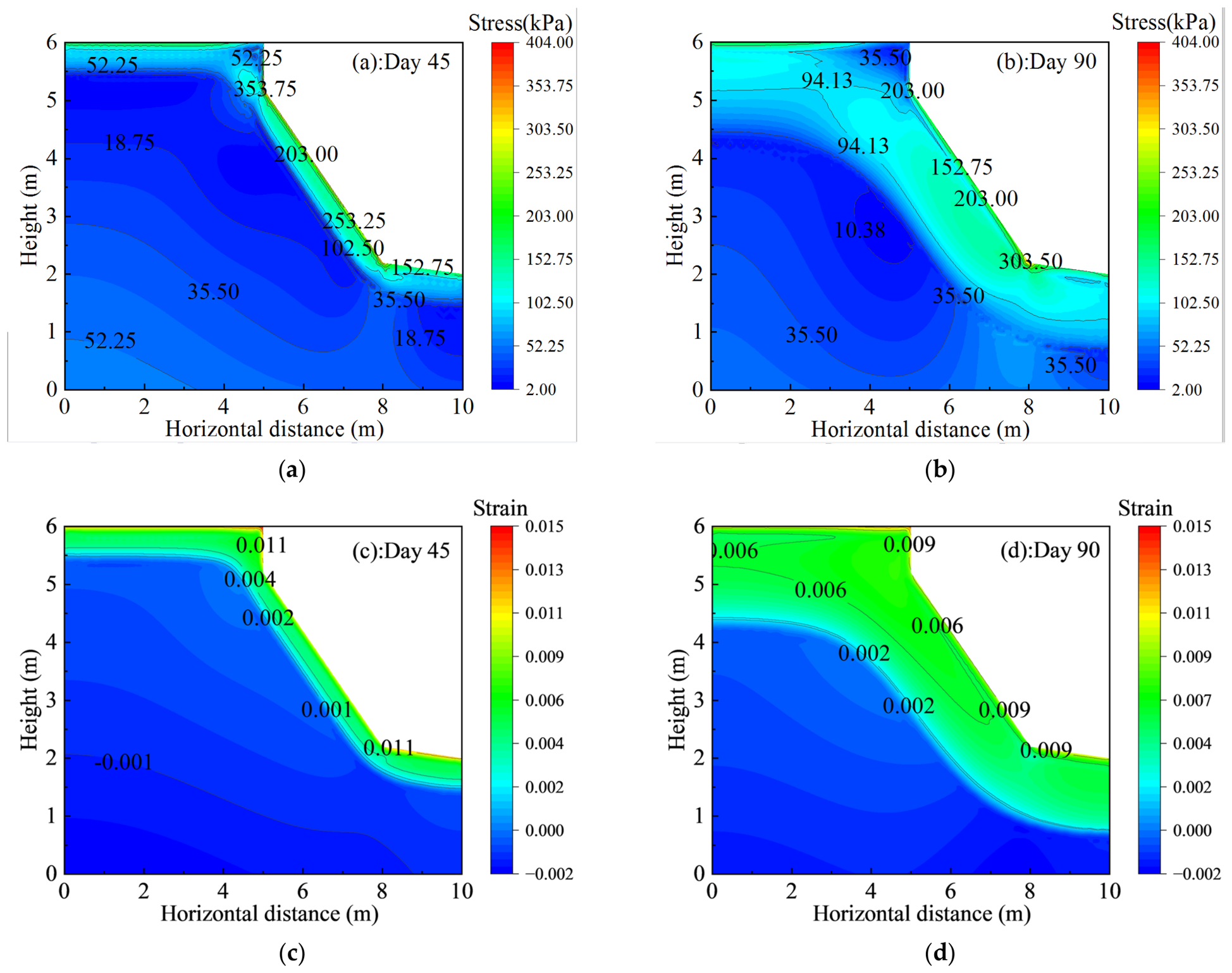
Figure 10 presents the spatial evolution of the stress and strain fields within the bank slope during the freeze–thaw process. As shown in Figure 10a,b, during the earlier freezing stage, relatively high stresses were mainly concentrated along the slope surface and in the upper part of the bank toe, whereas the stress contours within the interior of the slope remained comparatively smooth and the internal stress levels were generally low. By Day 90, corresponding to the deep-freezing stage, the stress field had undergone pronounced redistribution under the combined influence of sustained low-temperature boundary conditions and extensive freezing of the near-surface soil. Lateral compression and volumetric expansion induced by frost heave generated substantial additional stresses in the shallow slope and bank-toe regions. The originally low-stress region at the bank toe developed into a pronounced stress-concentration zone, where the peak stress exceeded 303.50 kPa.

Figure 10. Spatial evolution of stress and strain fields in the bank slope soil during freeze–thaw: (a) Day 45 stress; (b) Day 90 stress; (c) Day 45 strain; (d) Day 90 strain.

This strong stress concentration associated with water–ice phase transition and frost-heave deformation indicates a marked increase in the mechanical loading of the bank toe during the deep-freezing stage. The bank toe therefore represents a potentially vulnerable location in the subsequent warming and thawing period, during which stress redistribution and release may promote shear deformation and reduce slope stability.

Consistent with the evolution of the stress field, the strain field exhibited clear spatial migration and accumulation between Days 45 and 90, as shown in Figure 10c,d. At Day 45, during the early freezing stage, the exposed slope surface and crest responded first to the low-temperature boundary, producing frost-heave-induced tensile strains of approximately 0.011. Meanwhile, a slight compressive strain of approximately −0.001 developed within the slope interior, indicating that deformation was still mainly concentrated in the shallow near-surface soil.

By Day 90, corresponding to the peak frost-heave stage, the freezing front had propagated substantially downward into the soil mass. The zones of frost-heave-induced tensile strain along the slope surface and around the bank toe progressively expanded and became interconnected, while strain contours exceeding 0.006 extended further into the slope interior. The high-strain zone near the bank toe also expanded further. Although the maximum surface strain decreased slightly from 0.011 at Day 45 to 0.009 at Day 90, this reduction does not necessarily indicate an attenuation of the overall frost-heave deformation. Rather, together with the spatial expansion of the high-strain region, it suggests that deformation became progressively redistributed from a localized near-surface response toward a broader zone within the slope as freezing advanced.

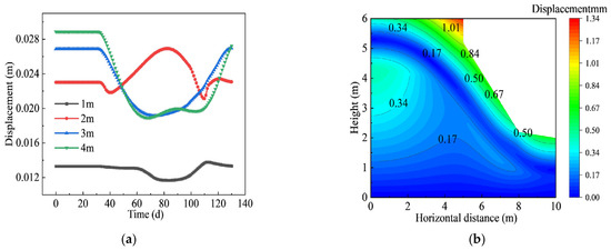
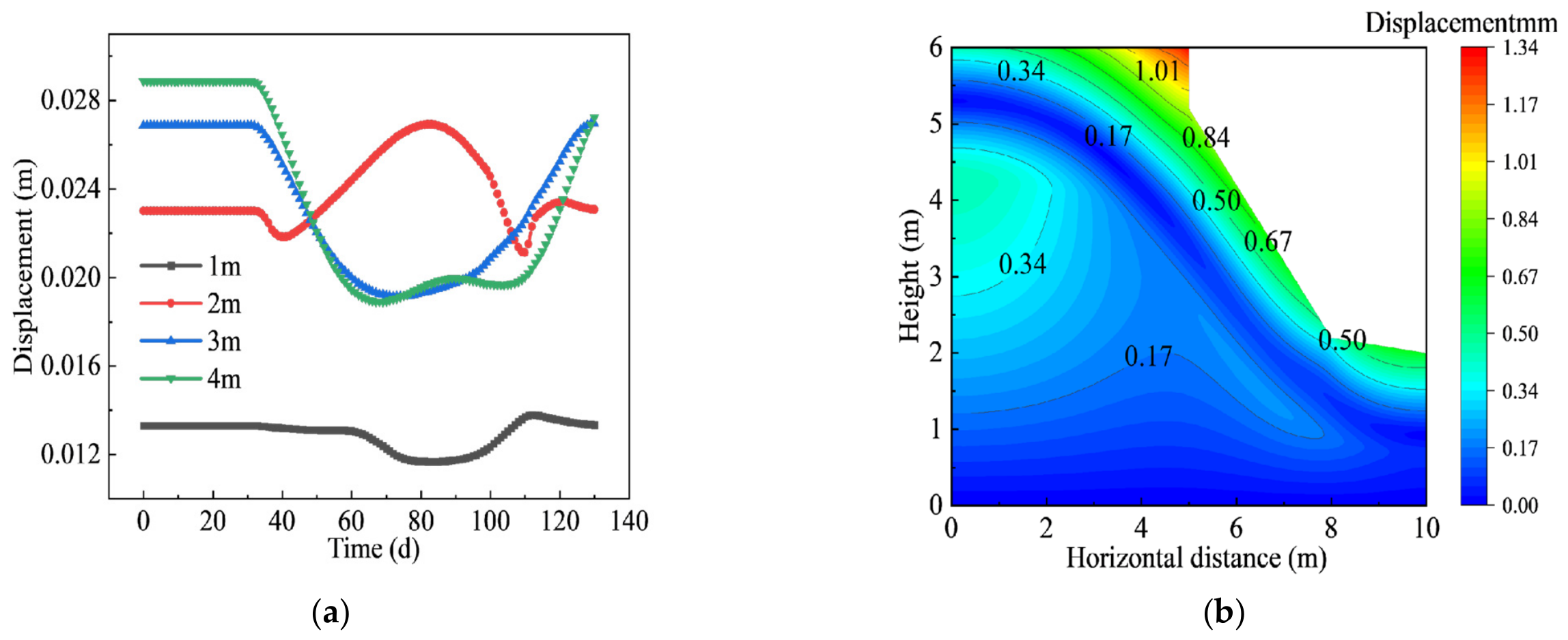
Figure 11 presents the time histories of cumulative displacement at different depths within the bank slope, together with the spatial distribution of displacement over the slope profile on Day 90. The displacement evolution curves indicate that the monitoring point at 1 m remained relatively stable throughout the simulation period, with only minor fluctuations, whereas the points at 2 m, 3 m, and 4 m exhibited pronounced dynamic responses. During the freezing period from Day 40 to Day 90, the displacements at 2 m, 3 m, and 4 m underwent successive sharp decreases or uplift-like fluctuations, reflecting structural adjustment of the soil induced by frost-heave-related volumetric change.

Figure 11. Displacement variation of bank slope during freeze–thaw and its spatial distribution contour map at the typical thawing period: (a) Displacement; (b) Contour map.

After Day 90, when the slope entered the thawing stage, especially during the interval from Day 90 to Day 120, the displacement curves at 2 m, 3 m, and 4 m all showed a distinct synchronous turning point followed by rapid increase, indicating that the thawing stage was associated with the most pronounced displacement variation during the entire freeze–thaw cycle. This intense displacement fluctuation suggests that, as air temperature rises and the near-surface frozen soil begins to thaw, the shallow bank soil undergoes a strong mechanical response under the combined influence of ice–water phase transition and soil–structure readjustment.

Because displacement variation was most pronounced during the thawing stage, the displacement field on Day 90 was selected for further spatial analysis. As shown in Figure 11b, the displacement field exhibits marked spatial heterogeneity. The upper-left corner of the slope crest and the shoulder region form the main displacement concentration zone, where the maximum displacement reaches 1.01 mm. Relatively large displacement bands, ranging from 0.50 mm to 0.84 mm, are also distributed along the exposed slope face and the middle-to-lower bank-toe region, whereas the deeper and inner parts of the slope show much smaller displacements, approximately 0.17 mm. These results indicate that, under the strong effect of thawing, the bank surface—particularly the slope shoulder and slope face—develops a clear tendency for outward deformation toward the free face.

The equivalent hydraulic head boundary formulated in the PDE framework typically exhibits lower numerical robustness compared with the native hydraulic head boundary in the built-in Darcy’s law interface. In this work, COMSOL’s Heat Transfer in Porous Media module is used for temperature field computation. Its porous medium component supports fluid type setup and phase-change material properties to directly describe ice–water phase change, while the porous matrix component permits assigning soil physical parameters separately for different soil layers. Thermal expansion coupling links the porous-media heat transfer field to the solid mechanics field, and poroelastic coupling realizes the interaction between the Darcy seepage field and solid mechanics field. In addition, the Darcy seepage velocity field is incorporated into the heat transfer interface to represent convective heat transport caused by moisture migration and sustain coupled information exchange between the thermal and Darcy seepage fields.

A saturation function is introduced, and the Van Genuchten soil–water characteristic curve is adopted to convert the temperature field into the liquid water content of the seepage field, thereby linking the temperature field and the Darcy seepage field.

$$S_e={\left[1+{\left(\alpha \left|h\right|\right)}^{1/(1-m)}\right]}^{-m}$$

(29)

where $S_e$ is the effective saturation, $h$ denotes the matric suction in kPa; $\alpha$ and m are the fitting parameters of the VG model, respectively.

To investigate the influence of lateral hydraulic boundaries on the freeze–thaw response of soil, a constant hydraulic head of 3 m is uniformly assigned on the left boundary of the model, which is derived from the multi-year average groundwater level of the river channel in the study area. Hydraulic heads of 2 m, 3 m and 4 m are applied on the right boundary of the model to represent working conditions under different water levels of the bank slope.

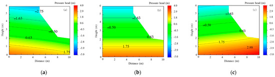
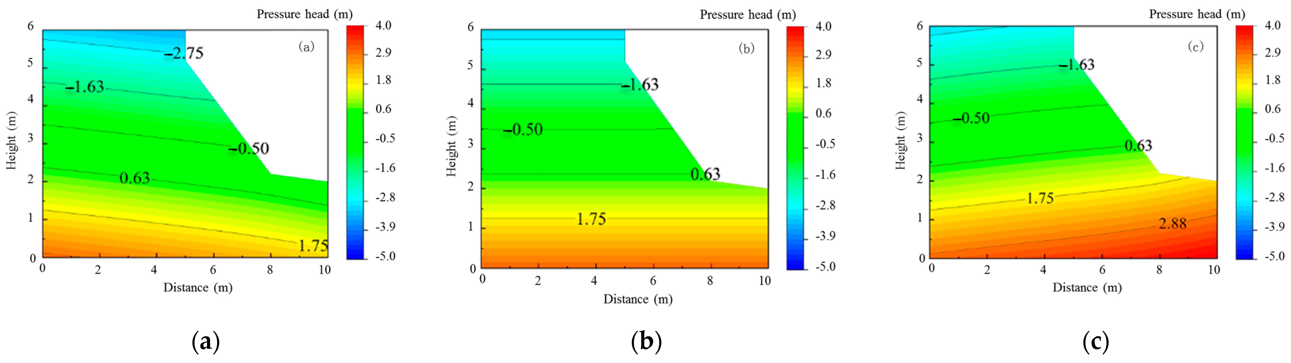
Figure 12 presents the contour plots of pressure head distribution in the slope under different water-level boundaries. It can be observed that when the river head on the right side is 2 m, the hydraulic head inside the left bank slope is higher than that on the river side, and seepage develops from the inner bank slope toward the river channel. A saturated zone with locally positive pressure head exists at the slope toe, while the pressure head of soil in the middle and upper parts of the slope are negative, indicating an unsaturated state. When the river head on the right rises to 3 m, the hydraulic head on the inner bank slope equals that on the river side, the lateral hydraulic gradient decreases significantly, and lateral seepage nearly disappears. The pressure head distribution of the slope is dominated by vertical variation. When the river head on the right increases to 4 m, the hydraulic head on the river side exceeds that inside the bank slope, and the seepage direction reverses. The region of high pressure head at the slope toe expands obviously, the saturated area in the lower slope enlarges, and the distribution range of negative pressure head and matric suction in the soil is compressed.

Figure 12. Contour plots of slope pressure head distribution under variable water head boundary conditions: (a) 2 m; (b) 3 m; (c) 4 m.

By comparing the three groups of working conditions, it can be seen that the variation of river-side hydraulic head can significantly alter the spatial distribution of pressure head, the extent of saturated zones and the seepage direction inside the slope. As the river-side hydraulic head rises, the pore water pressure of slope soil increases overall, the saturated zone expands upward, and the matric suction of soil decreases. Changes in pore water pressure affect the pattern of moisture migration during freeze–thaw processes, thereby modifying the mechanical properties of slope soil and exerting a substantial influence on bank slope stability under freeze–thaw conditions.

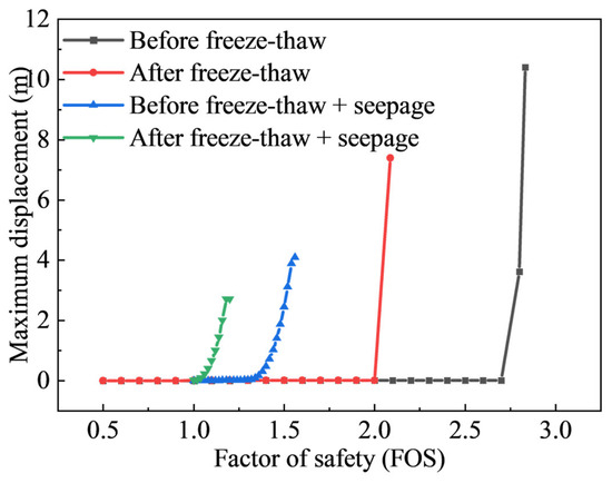
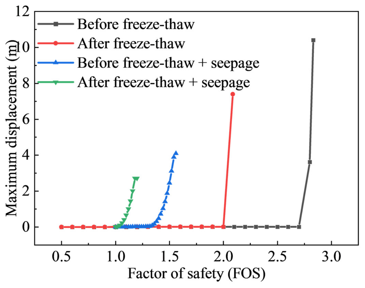
Figure 13 presents the relationship between the factor of safety and maximum displacement of the bank slope under different conditions. Under the original natural condition without freeze–thaw or seepage effects, the bank slope exhibited the highest stability margin, with a factor of safety of approximately 2.8. After one freeze–thaw cycle, deterioration of the soil structure resulted in a pronounced decrease in the factor of safety to approximately 2.05. When seepage was considered, the factor of safety further decreased to approximately 1.4 because pore water pressure generated by groundwater reduced the effective stress within the soil, bringing the slope closer to a critical stability state.

Figure 13. Variation of safety factor with maximum displacement of bank slope under different working conditions.

When freeze–thaw and seepage effects were considered simultaneously, the factor of safety decreased markedly to approximately 1.1, well below the adopted stability control threshold of 1.3 [33,34]. Comparison of the four conditions indicates that slope stability is jointly controlled by freeze–thaw and seepage effects, and that their combined action produces a stronger reduction in stability than either process considered individually.

From a mechanistic perspective, freeze–thaw action may promote the development of microcracks within the soil, providing preferential pathways for subsequent seepage. Seepage, in turn, can weaken the soil structure and intensify freeze–thaw-induced deterioration. The interaction between these processes may therefore progressively reduce the stability of the bank slope and increase its susceptibility to overall sliding failure during the spring thaw period.

5. Conclusions and Limitations

5.1. Conclusions

This study investigated the embankments along the Inner Mongolia reach of the Yellow River, which are strongly affected by seasonal freeze–thaw processes. Basic physical tests and multivariable mechanical tests were conducted on sampled soils to examine the effects of freeze–thaw cycling, water content, and related factors on soil mechanical behavior. A thermo-hydro-mechanical (THM) coupled model for riverbank stability was subsequently developed, validated, and applied to the stability analysis of a typical riverbank cross-section. The main conclusions are as follows:

(1) Compared with water content and the number of freeze–thaw cycles, dry density was the dominant factor controlling soil shear strength. The soil exhibited its highest shear strength near the optimum water content. Increasing the number of freeze–thaw cycles caused pronounced degradation of soil cohesion, with the most substantial reduction occurring during the first three cycles; the rate of degradation decreased thereafter. By contrast, the internal friction angle was much less sensitive to freeze–thaw cycling.

(2) The developed THM coupled model satisfactorily reproduced the evolution of temperature, moisture, and displacement within the soil during freezing and thawing. When applied to the typical riverbank cross-section, the model captured the continuous evolution of the internal stress–strain response and displacement throughout the freeze–thaw period, identified the bank toe and near-surface slope regions as the most unfavorable locations for stability, and quantified variations in the factor of safety under different stages and influencing conditions.

5.2. Limitations

This study investigates the mechanical behaviors of silty sand under different freeze–thaw cycles, water contents and dry densities, and analyses the stability of the typical embankment at Shisifenzi under hydrothermal–mechanical coupling. The experimental and modeling results not only provide parameter references for sustainable resilient design and hazard-risk evaluation of seasonally frozen river embankments, but also facilitate risk-informed decision-making for cold-region river hazard mitigation and support the sustainable operation of flood-protection infrastructures. However, the Yellow River (Inner Mongolia reach) extends approximately 840 km. The embankments at different locations differ in soil physico-mechanical properties, bank slope geometry, groundwater conditions and inter annual temperature variations, leading to discrepancies in the deterioration mechanisms and instability laws under multi-factor coupling.

In the laboratory tests on freeze–thaw mechanical properties, the freeze–thaw boundary conditions and UU triaxial tests adopted in this study have limitations in capturing the dynamic evolution of soil behavior. Future work will carry out comprehensive stability analyses for embankment soils and slope configurations from different regions. The actual variable temperature histories and freeze–thaw cycle characteristics of in situ soils will be considered, and internal soil parameters including pore water pressure, temperature, water content and deformation will be monitored. More accurate CU or CD triaxial tests and frost-heave tests will be performed to calibrate parameters such as the frost-heave initiation threshold. Quantitative analysis of the evolution of soil micro-pore structures during freeze–thaw will be conducted using CT or SEM. These efforts will further strengthen the experimental basis for hydro-mechanical coupling processes and help clarify the freeze–thaw mechanisms and stability characteristics of embankment soils along the entire Yellow River (Inner Mongolia reach).

Meanwhile, the linear elastic constitutive relation combined with the Mohr–Coulomb strength criterion used herein cannot fully describe the nonlinearity, path dependence and irreversible cumulative plastic deformation of soil subjected to repeated freeze–thaw cycles. Subsequent research will introduce elastoplastic constitutive models or freeze–thaw damage models to more realistically simulate irreversible deformation and stiffness degradation.

References

- Formanek, G.E.; Mccool, D.K.; Papendick, R.I. Freeze-Thaw and Consolidation Effects on Strength of a Wet Silt Loam. Trans. ASAE 1984, 27, 1749–1752. [Google Scholar] [CrossRef] [Scilit]
- Xiao, J.; Sun, B.; Li, Z.; Zhang, L.; Ma, B. Effects of freeze-thaw cycles on Aeolian sand soil physical properties and soil anti-scourability. J. Soil Water Conserv. 2017, 31, 67–71. [Google Scholar] [CrossRef]
- Aoyama, K.; Ogawa, S.; Fukuda, M. Temperature dependencies of mechanical properties of soils subjected to freezing and thawing. In Proceedings of the 4th International Symposium, Sapporo, Japan, 5–7 August 1985; CRC Press: Boca Raton, FL, USA, 1985. [Google Scholar] [CrossRef] [Scilit]
- Ogata, N.; Kataoka, T.; Komiya, A. Effect of freezing-thawing on the mechanical properties of soil. In Proceedings of the 4th International Symposium, Sapporo, Japan, 5–7 August 1985; CRC Press: Boca Raton, FL, USA, 1985. [Google Scholar] [CrossRef] [Scilit]
- Dong, X.; Zhang, A.; Lian, J.; Guo, M. Study of shear strength deterioration of loess under repeated freezing-thawing cycles. J. Glaciol. Geocryol. 2010, 32, 767–772. [Google Scholar] [CrossRef]
- Li, L.; Zhang, K.; Zhang, Q.; Mao, Y.; Li, G. Experimental study on the loess strength degradation characteristics under the action of dry-wet and freeze-thaw cycles. J. Glaciol. Geocryol. 2016, 38, 1142–1149. [Google Scholar] [CrossRef]
- Gandah, L.R. The Damaging Effects of Frost Action in Roads, Over-View of Types of Damage and Preventive Measures; VTI Report no. 230; Swedish Road and Traffic Research Institute: Linkoping, Sweden, 1980; Volume 13, pp. 418–423. [Google Scholar]
- Yu, J.; Wang, N.; Tan, F.; Wei, H.; Fu, W. Experimental investigation on mechanical behaviors of saturated silty clay under freeze-thaw cycles. Geotech. Eng. World 2008, 11, 48–51. [Google Scholar]
- Yu, J. Design of Low Temperature Triaxial Testing Machine and Experimental Study on Cyclic Freeze-Thaw on the Mechanical Properties of Silty Clay. Ph.D. Thesis, The Chinese Academy of Sciences (Wuhan Institute of Rock and Soil Mechanics), Wuhan, China, June 2007. [Google Scholar]
- Weeks, A.G. The stability of natural slopes in south-east England as affected by periglacial activity. Q. J. Eng. Geol. 1969, 2, 49–63. [Google Scholar] [CrossRef] [Scilit]
- Hutchinson, J.N. Periglacial solifluxion: An approximate mechanism for clayey soil. Geotechnique 1974, 24, 438–443. [Google Scholar] [CrossRef] [Scilit]
- Ji, D.; Niu, F.; Chen, Z.; Ni, W. Discussion on method of stability analysis of infinite slope for different seepage conditions. J. Geol. Hazards Environ. Preserv. 2003, 14, 63–67. [Google Scholar]
- Pufahl, D.E.; Morgenstern, N.R. Stabilization of planar landslides in permafrost. Can. Geotech. J. 1979, 16, 734–747. [Google Scholar] [CrossRef] [Scilit]
- Morgenstern, N.R.; Price, V.E. The Analysis of the stability of general Slip Surfaces. Géotechnique 1965, 15, 79–93. [Google Scholar] [CrossRef] [Scilit]
- Zhou, X.P.; Cheng, H. The long-term stability analysis of 3D creeping slopes using the displacement based rigorous limit equilibrium method. Eng. Geol. 2015, 195, 292–300. [Google Scholar] [CrossRef] [Scilit]
- Ugai, K.; Leshchinsky, D. Three-dimensional limit equilibrium and finite element analyses: A comparison of results. J. Jpn. Geotech. Soc. 1995, 35, 1–7. [Google Scholar] [CrossRef] [Scilit]
- Wei, W.; Cheng, Y. A temperature-driven strength reduction method for slope stability analysis. Mech. Res. Commun. 2009, 36, 224–231. [Google Scholar] [CrossRef] [Scilit]
- Zhang, J.; Lai, Y.; Zhang, M.; You, Z. Study on the coupling mechanism of water-heat-vapor-salt-mechanics in unsaturated freezing sulfate saline soil. Comput. Geotech. 2024, 169, 106232. [Google Scholar] [CrossRef] [Scilit]
- Luo, H.; Ji, H.; Gao, G.; Zhang, B.; Mou, X. Study on the characteristics of flow and ice jam in Shisifenzi bend in the Yellow River during the freeze-up period. J. Hydraul. 2020, 51, 1089–1100. [Google Scholar] [CrossRef]
- Zhao, S.; Li, C.; Li, C.; Shi, X.; Zhao, S. Processes of river ice and ice-jam formation in Shensifenzi Bend of the Yellow River. J. Hydraul. Eng. 2017, 48, 351–358. [Google Scholar] [CrossRef]
- GB/T 50123-2019; Standard for Geotechnical Test Methods. China Planning Press: Beijing, China, 2019.
- Tian, H. Variation characteristics of temperature in Hohhot city in recent 30 years and its impacts on agricultural production. South China Agric. 2021, 15, 197–199. [Google Scholar] [CrossRef]
- Tao, W. Heat Transfer; Higher Education Press: Beijing, China, 2019. [Google Scholar]
- Lu, N.; Likos, W.J. Unsaturated Soil Mechanics; Wei, C.; Hou, L.; Jian, W., Translators; Higher Education Press: Beijing, China, 2012. [Google Scholar]
- Taylor, G.S.; Luthin, J. A model for coupled heat and moisture transfer during soil freezing. Can. Geotech. J. 1978, 15, 548–555. [Google Scholar] [CrossRef] [Scilit]
- Wang, X. Study on Characteristics of Frost Heave and Thawing Settlement of Pile-Soil System in Permafrost Regions. Master’s Thesis, Xi’an University of Science and Technology, Xi’an, China, June 2019. [Google Scholar]
- Bai, Q.; Li, X.; Tian, Y.; Fang, J. Equations and numerical simulation for coupled water and heat transfer in frozen soil. Chin. J. Geotech. Eng. 2015, 37, 131–136. [Google Scholar] [CrossRef]
- Xu, X.; Deng, Y. Experimental Study on Water Migration in Freezing and Frozen Soils; Science Press: Beijing, China, 1991. [Google Scholar]
- He, L. Mechanical Properties and Numerical Analysis of Fiber Gangue Composite Improved Soil Under Freeze-Thaw Cycle. Master’s Thesis, Inner Mongolia Agricultural University, Hohhot, China, June 2021. [Google Scholar] [CrossRef]
- Bai, Q. Determination of Boundary Layer Parameters and a Preliminary Research on Hydrothermal Stability of Subgrade in Cold Region. Master’s Thesis, Beijing Jiaotong University, Beijing, China, December 2015. [Google Scholar]
- Lu, S. Experimental and Numerical Simulation Analysis of Water-Heat Migration of Silty Sand in Cold Regions Under Freezing Action. Master’s Thesis, Heilongjiang University, Harbin, China, May 2020. [Google Scholar] [CrossRef]
- Zhang, L.; Zheng, Y.; Zhao, S.; Shi, W. The feasibility study of strength-reduction method with FEM for calculating safety factors of soil slope stability. J. Hydraul. Eng. 2003, 1, 21–27. [Google Scholar] [CrossRef]
- Stark, T.D.; Ruffing, D.G. Selecting minimum factors of safety for 3D slope stability analyses. In Geo-Risk 2017: Geotechnical Risk Assessment and Management; American Society of Civil Engineers: Reston, VA, USA, 2017; pp. 259–266. [Google Scholar] [CrossRef] [Scilit]
- Li, C.; Yang, Z.; Shen, H.T.; Mou, X. Freeze-Thaw Effect on Riverbank Stability. Water 2022, 14, 2479. [Google Scholar] [CrossRef] [Scilit]
Disclaimer/Publisher’s Note: The statements, opinions and data contained in all publications are solely those of the individual author(s) and contributor(s) and not of MDPI and/or the editor(s). MDPI and/or the editor(s) disclaim responsibility for any injury to people or property resulting from any ideas, methods, instructions or products referred to in the content. |
© 2026 by the authors. Licensee MDPI, Basel, Switzerland. This article is an open access article distributed under the terms and conditions of the Creative Commons Attribution (CC BY) license.