Water Quality in the Haihe River Basin, China: Spatial and Seasonal Variations, Sources and Sustainable Strategies

Abstract

A two-year dataset was collected to investigate the spatial and seasonal variations in water quality within the Haihe River Basin (HRB), China. Potential pollution sources and influencing factors were identified, and their contributions were quantified using absolute principal component scores-multiple linear regression (APCS-MLR) and Positive Matrix Factorization (PMF) models. The average water quality index (WQI) was 80.2, indicating that the overall water quality was classified as “good”. TN pollution was severe. WQI values followed the order: Luanhe River system (84.7) > North Haihe River system (80.0) > South Haihe River system (76.6). The WQI value during the non-flood season (77.2) was lower than that during the flood season (82.0). Grassland and forest exhibited negative correlations with water-quality parameters. Construction land and farmland negatively influenced water quality but were not the primary land-use types contributing to TN variability. Higher pH and TN occurred in mountain areas and during the non-flood season, while higher COD_Mn, COD, BOD, AN, and TP occurred in plain areas and estuaries, respectively, and during the flood season. Four potential sources or factors were identified as domestic and industrial wastewater, meteorological and hydrological conditions as environmental driving factors, non-point sources, and unrecognized sources. Source apportionment using APCS-MLR and PMF models revealed that domestic and industrial wastewater contributed 28.6% and 47.2% of pollution, respectively, while non-point sources contributed 27.7% and 22.2%. Meteorological and hydrological conditions, as environmental driving factors, accounted for 17.9% and 21.0% of the variability, respectively, and unrecognized sources accounted for 25.8% and 9.6%. Sustainable control strategies were proposed to improve water quality in the HRB in the future.

1. Introduction

Water quality is a global environmental issue because it significantly affects natural ecosystems and human well-being. Increasing pollutant discharges from industrial, municipal, and agricultural sources have caused severe water contamination, and most river basins in China face significant challenges in reducing pollutants [1]. Water quality is influenced not only by anthropogenic factors (e.g., domestic and industrial wastewater, land use, agricultural activities) but also by natural factors (e.g., environmental conditions, climate change) [2]. Rapid urbanization and modernization have created notable challenges related to sewage treatment and water quality [3]. Land-use patterns are key determinants of water quality, and farmland has exerted substantial influence on water quality in numerous river basins. Land-use changes directly alter concentrations of water pollutants such as turbidity (Turb), electrical conductivity (EC), ammonia–nitrogen (AN), permanganate index (COD_Mn), and Fe²⁺ in built-up and forested areas [2]. Land use affects urban river water quality with distinct seasonal variations and spatial-scale dependencies. Studies have found both negative and positive correlations between water quality parameters and land use patterns in non-flood and flood seasons [4]. To address water pollution and improve water quality, China has implemented national action plans for water pollution control and prevention. These comprehensive abatement measures aim to substantially reduce the concentrations of AN, chemical oxygen demand (COD), total nitrogen (TN), and total phosphorus (TP) across diverse river basins [5,6]. Assessing the effectiveness of these measures in reducing pollutant concentrations carries meaningful policy implications for future water quality improvement [5]. Basin-scale spatial patterns of water quality can provide essential insights for sustainable regional water resource management [7]. This study used the Haihe River Basin (HRB) as a case to explore spatial and seasonal changes in surface water quality and identify possible pollution sources and driving factors. As the first systematic evaluation of these plans, the present research provides an empirical reference for other river basins to optimize environmental protection regulations.

The aims of the current research are: (1) to evaluate surface water quality and examine its spatial and seasonal changes in the HRB; (2) to investigate the relationship between surface water quality parameters and land use patterns in the HRB; (3) to identify possible pollution sources and factors and obtain a source apportionment of contributions to water pollution in the HRB. Ultimately, this study provides a scientific basis for formulating systematic pollution-control strategies and water-quality management regulations in the HRB.

2. Materials and Methods

2.1. Study Area

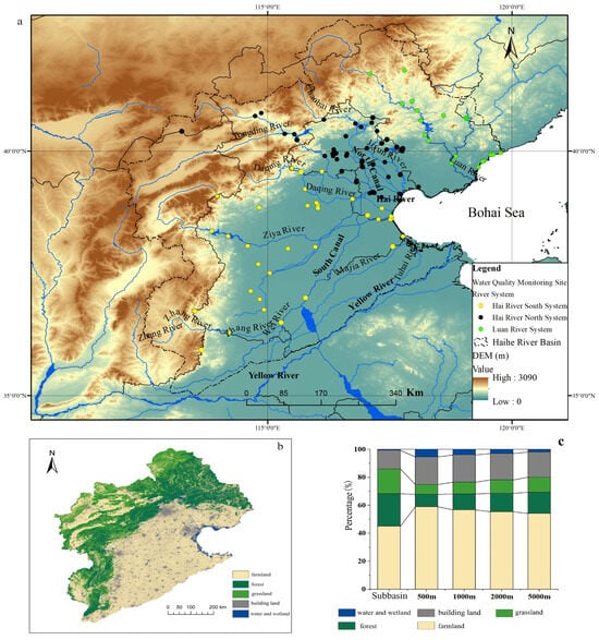
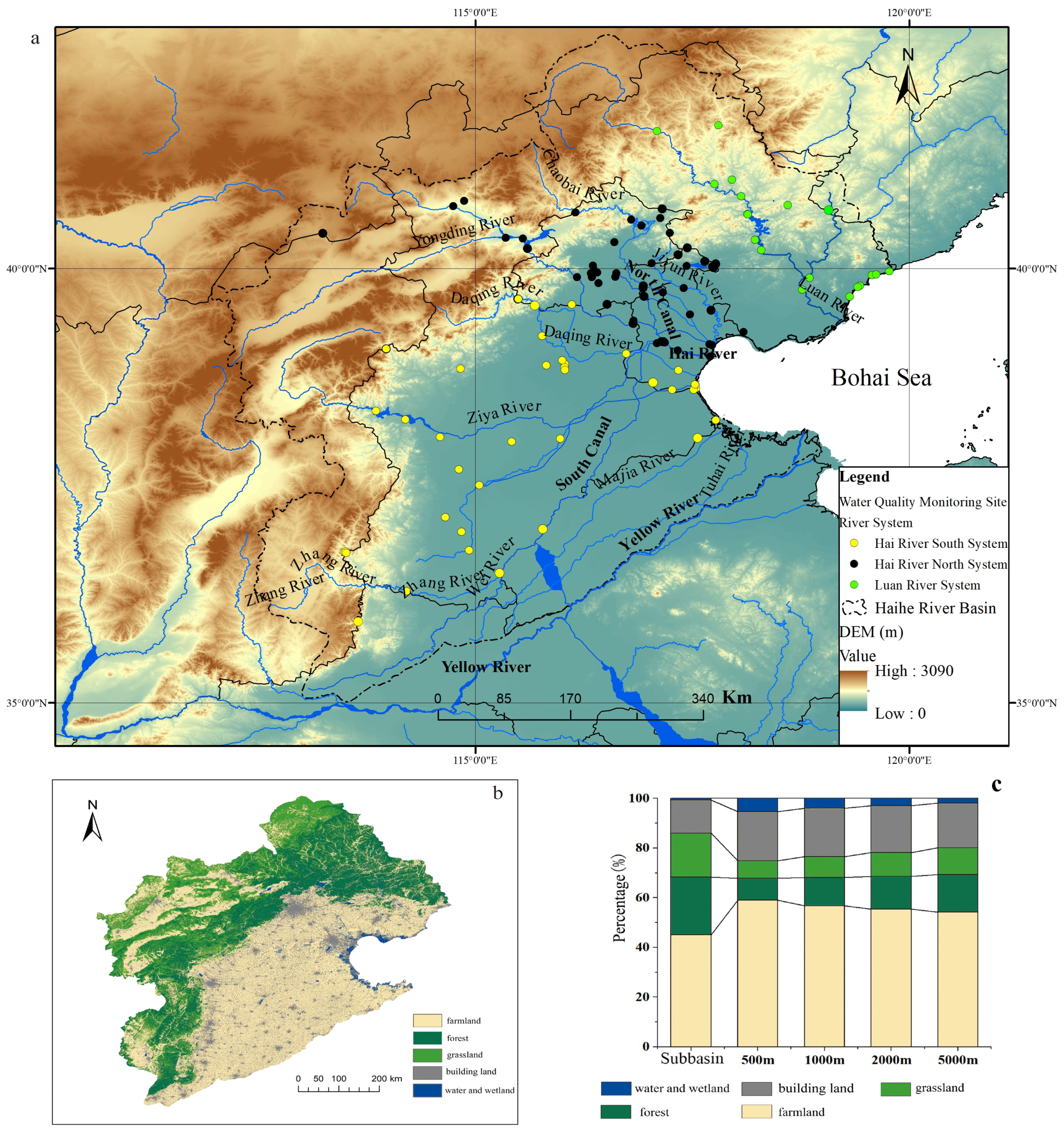
The Haihe River Basin (HRB) spans one autonomous region, two municipalities, and five provinces in northern China. The basin is 31.82 × 10⁴ km², accounting for 3.3% of China’s land area. The terrain slopes from southeast to northwest, with low elevation in the southeast and high elevation in the northwest (Figure 1a). The HRB consists of plateau and mountains (1.89 × 10⁴ km², 60%) and plains (1.29 × 10⁵ km², 40%). The Bohai Sea borders it to the east, the Taihang Mountains to the west, the Yellow River to the south, and the Inner Mongolia Plateau to the north. The basin has a semi-humid, semi-arid continental East Asian monsoon climate, with mean annual precipitation of 539 mm and mean annual air temperature ranging from approximately 1.5 to 14 °C (1956–1998) [8]. In the present study, the HRB was divided into three major river systems: Luanhe River system (Luan River, with sampling sites indicated by green dots), North Haihe River system (North HR, with sampling sites indicated by black dots, including North Canal, Yongding River, Chaobai River, and Jiyun River), and South Haihe River system (South HR, with sampling sites indicated by yellow dots, including Daqing River, Ziya River, Zhang River, Wei River, South Canal, Tuhai River, and Majia River. Because of topographic heterogeneity, land-use patterns in the HRB differ significantly between the northwest and southeast. Cultivated land is the dominant land use type, mainly distributed in the middle and lower reaches and in low-lying areas of the western mountainous areas. Forest and grassland are concentrated in the western and northern mountainous zones. Meanwhile, built-up land is mainly distributed in the eastern plains, forming two core agglomerations in Beijing and Tianjin. We extracted 82 subbasins and buffer zones (500 m, 1000 m, 2000 m, and 5000 m) around each sampling site using the hydrological analysis module in ArcGIS 10.3 (Esri, Redlands, CA, USA) and a 30 m resolution Digital Elevation Model (DEM) obtained from Geospatial Data Cloud (Chinese Academy of Sciences, Beijing, China). Figure 1b,c show the statistical analysis of land use across the entire HRB, buffer zones, and subbasins. Farmland was the largest land use type in the sub-basins, accounting for about 45%, with an average proportion exceeding 50%. As the buffer scale increased, the proportion of farmland gradually decreased, while the percentages of forest and grassland areas increased correspondingly.

Figure 1. Overview and land-use characteristics in the HRB. (a) Water quality monitoring sites and river systems; (b) Land use/land cover map; (c) Percentage composition of different land-use types across the subbasin and different buffer zones.

2.2. Data Collection

A total of 25 physicochemical water quality parameters were collected during 2021–2022 for analysis, including pH, water temperature (WT), EC, Turb, dissolved oxygen (DO), biochemical oxygen demand (BOD), COD_Mn, COD, TP, AN, TN, Zn, Cu, Hg, Cd, Cr⁶⁺, Pb, As, Se, fluoride (F⁻), sulfide (S²⁻), oil pollutants, cyanide (CN), volatile phenolic compounds (VPCs), and linear alkylbenzene sulfonates (LAS). Data were sourced from China’s 14th Five-Year Plan national surface water environmental quality monitoring database (https://data.epmap.org/page/index) (accessed on 15 October 2024). A total of 98 sampling sites were distributed across the three river systems: 18 in the Luan River, 45 in the North HR, and 35 in the South HR. Each site was monitored once a month. The dataset was divided into flood-season and non-flood-season subsets. In China, the flood season is conventionally differentiated between the southern and northern regions: in the southern basins (Yangtze, Pearl River, and Taihu Lake basins), the flood season spans April to October with a main flood season from June to August, whereas in the northern basins (Yellow, Huai, Hai, Songhua, and Liao River basins), the flood season spans June to September with a main flood season from July to August. Because the HRB belongs to the northern group, this study defined the flood season as June to September and the non-flood season as October to May. We obtained a 10 m × 10 m gridded land-use dataset for the HRB from Geospatial Data Cloud (https://www.gscloud.cn/) (accessed on 15 August 2024). Land use was commonly categorized into five categories: farmland, forest, grassland, built-up land, and water/wetland. A 30 m resolution DEM was sourced from the Geographical Information Monitoring Cloud Platform (GIM Cloud, http://www.dsac.cn/) (accessed on 15 December 2024).

2.3. Methods

Normal distribution hypotheses of water quality parameters were tested using the Shapiro–Wilk (S-K) and Kolmogorov–Smirnov (K-S) tests. One-way ANOVA was applied to verify spatial and seasonal variation in pollutant concentrations, including differences between flood and non-flood seasons, across three landscape zones (mountain areas, plain areas, and estuaries), and among three water systems (Luan River, North HR, and South HR). Before ANOVA, the homogeneity of variances was assessed using Levene’s test. Because we performed multiple ANOVA comparisons, we controlled the family-wise Type I error rate by applying post hoc multiple comparison corrections (e.g., Bonferroni) to the pairwise comparisons and interpreted the results conservatively. We calculated the areas of farmland, grassland, forest, built-up land, and water/wetland within 500 m, 1000 m, 2000 m, and 5000 m buffers and subbasins surrounding each sampling site using buffer analysis and area tabulation tools in ArcGIS 10.1. Redundancy analysis (RDA) was used to explore the impact of land use on water quality at multiple spatial scales (subbasin, 500 m, 1000 m, 2000 m, and 5000 m) across four periods (annual, dry, normal, and wet seasons). The relationship between land-use types and water quality parameters was analyzed using RDA in IBM SPSS Statistics 26.0.

(1)

Water quality index (WQI)

WQI is a convenient and valuable method of evaluating water quality in river reaches, watersheds, and bays. The detailed calculation procedure and assigned relative weights of parameters were provided in a previous study [9]:

$$\mathrm{WQI}={\displaystyle \frac{{\sum }_{i=1}^n{W_{i}Q}_i}{{\sum }_{i=1}^n{W}_i}}$$

(1)

where W_i is the weight given from 1 to 4 to each parameter, Q_i is the value given to each parameter after standardization, and n is the total number of parameters (Table S1). WQI ranged from 0 to 100, with lower values indicating worse water quality and higher values indicating better water quality. Classification criteria are as follows: excellent (91 ≤ WQI ≤ 100), good (71 ≤ WQI < 90), medium (51 ≤ WQI < 70), bad (26 ≤ WQI < 50), and very bad (0 ≤ WQI < 25) [9]. In this study, WQI was calculated using pH, T, EC, DO, Turb, BOD, COD, AN, TP, and TN. The ten parameters were selected because they (i) represent the major conventional physicochemical groups routinely used in surface water quality assessment, namely physicochemical indicators (pH, T, EC), oxygen-related indicators (DO, BOD, COD), nutrient indicators (AN, TP, TN), and turbidity; (ii) are the core indicators of both the Chinese national surface water environmental quality standard (GB 3838-2002) [10] and the applied WQI scheme [9]; and (iii) had complete monitoring coverage across all 98 sampling sites. Heavy metals and toxic organic compounds were also measured but excluded from the WQI because the applied WQI framework is based on conventional water-quality indicators [9]. The relative weights (W_i, ranging from 1 to 4) were assigned according to the relative importance of each parameter for water quality and for ecosystem and human health as defined in the WQI scheme [9]; parameters with stronger implications for water use and aquatic health (e.g., DO, BOD, AN, TP, and TN) received higher weights, whereas parameters with secondary influences (e.g., T and Turb) received lower weights.

(2)

PCA-APCS-MLR

High-dimensional datasets are widespread in water environment research. Principal component analysis (PCA) effectively reduces the dimensionality of original datasets. PCA was first adopted to identify the possible sources and driving factors of water pollution. Absolute principal component score (APCS) was then derived from PCA results. Finally, a multiple linear regression (MLR) model was established between the independent variable (APCS) and the dependent variables (water quality parameters) to quantify source contributions. The APCS-MLR is expressed as:

$${\mathit{APCS}}_{\mathit{jk}}={\left(A_Z\right)}_{\mathit{jk}}-{\left(A_0\right)}_k$$

(2)

$$C_j=a_k+{\displaystyle {\sum }_{k=1}^k}{b}_{\mathit{jk}}\times {\mathit{APCS}}_{\mathit{jk}}$$

(3)

where (A_z)_jk is the score of the principal component, (A₀)_k is the corresponding score for the principal component, C_j represents the measured concentration of pollutant j, b_jk is the multiple regression coefficient of pollutant source k on pollutant j, b_jk × APCS_jk is the contribution of source k to C_j, and a_k is the multiple regression constant term. Detailed descriptions were provided by Haji Gholizadeh [11]. PCA was considered valid when Bartlett’s sphericity (k < 0.05) and the Kaiser–Meyer–Olkin statistic (KMO > 0.5) tests were satisfied. A cumulative variance contribution > 55% was regarded as acceptable [12]. Factor loadings were defined as weak (0.3–0.5), moderate (0.5–0.75), and strong (>0.75).

(3)

PMF model

The PMF model was applied to identify and quantify surface water pollution sources [13]. The original dataset (X) was decomposed into a factor distribution matrix (F), a factor contribution matrix (G), and a residual matrix (E). The PMF model can be expressed as:

$$X_{\mathit{ij}}=E_{\mathit{ij}}+{\displaystyle {\sum }_{p=1}^k}{G}_{\mathit{ip}}\times F_{\mathit{pj}}\left(i=1,2,\cdots ,n,j=1,2,\cdots ,m\right)$$

(4)

where X_ij is the concentration for each sample, E_ij is the residual for each sample, G_ip is the amount of mass contributed by each factor (p) to each sample (i), F_kj is the species profile of each source, p is the number of factors, n is the number of samples, and m is the number of chemical species. All values of G and F are non- negative.

The objective function Q is minimized based on residuals and uncertainties:

$$Q={\displaystyle {\sum }_{i=1}^n}{\displaystyle {\sum }_{j=1}^m}\left({\displaystyle \frac{E_{\mathit{ij}}}{U_{\mathit{ij}}}}\right)$$

(5)

where U_ij is the uncertainty associated with each species measurement.

The number of factors (p) was determined by evaluating the convergence and stability of the objective function Q across different factor numbers and random initial seeds, combined with the physical interpretability of the resulting factor profiles and their consistency with the PCA-APCS-MLR results; a three-factor solution provided the best compromise between model fit and interpretability and was therefore retained. Uncertainties were propagated in the PMF model using the standard error model [13], which accounts for both analytical uncertainty and the method detection limit (MDL). Concentrations below the MDL were substituted with half of the MDL, and their uncertainties were estimated using the standard PMF error-estimation procedure [13].

3. Results and Discussion

3.1. Statistics and Water Quality Assessment

Descriptive statistics for water quality parameters in the HRB were analyzed to characterize data variability (Table S2). Skewness and kurtosis were used to test normality. Positive skewness values showed that the parameters, except T, were non- normally distributed and right skewed. The K-S and S–W tests confirmed non-normal distributions (p < 0.001). Kurtosis values for T, pH, COD_Mn, COD, and BOD were <3, while those for other parameters were >3, indicating sharper peaks and longer tails than a normal distribution. Natural factors (precipitation, surface runoff, river flux) and human activities (industrial and population growth, agricultural activities, urbanization) can affect parameter distributions. In well-mixed natural waters, variables typically follow normal distributions. Concentration distributions reflect pollutant emissions, transport, sources, and sinks, excessive pollutant discharges often lead to right-skewed distributions because of sporadic high-value observations [14]. The detailed normality statistics (Shapiro–Wilk and Kolmogorov–Smirnov statistics, skewness, and kurtosis) for all parameters are provided in Table S2.

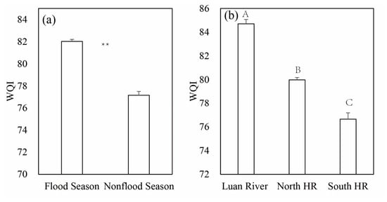
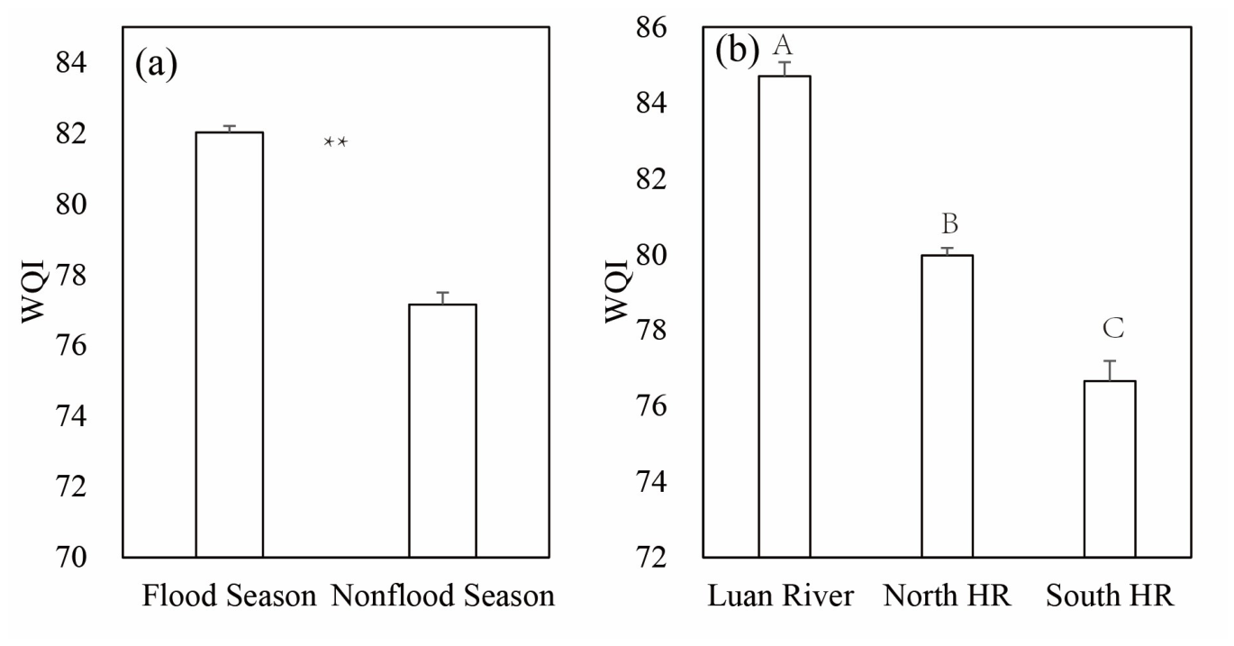
WQI values based on the ten parameters (pH, T, EC, DO, Turb, BOD, COD, AN, TP, and TN) were calculated for different water systems and seasons (Figure 2). The mean WQI for the HRB was 80.2, indicating “good” water quality. ANOVA results indicated significant seasonal and spatial differences in WQI (p < 0.01). WQI was significantly lower in the non-flood season (77.2) than in the flood season (82.0). Among river systems, WQI followed the order: Luan River (84.7) > North HR (80.0) > South HR (76.6) (p < 0.01).

Figure 2. WQI values in different water seasons (a) and water systems (b) (different uppercase letters in the different columns indicate significant differences (p < 0.01), and ** indicates significant differences (p < 0.01)).

Water quality parameters were evaluated against the Chinese Class III Surface Water Environmental Quality Standard (GB 3838-2002) [10]. All parameters except TN met the standard. TN concentrations ranged from 4.21 to 6.62 mg/L (mean = 4.43 mg/L), making TN the primary pollutant in the HRB. Xiong reported that the HRB had the highest TN levels among China’s 10 major river basins, with annual averages exceeding 3.3 mg/L in the Beijing–Tianjin–Hebei region [1]. Xie reported TN concentrations in estuaries across China of 3.24 ± 2.73, 3.60 ± 2.55, and 3.92 ± 3.30 mg/L in 2020, 2021, and 2022, respectively [15]. Primary sources of TN include soil nitrogen, litter, sewage effluents, atmospheric deposition, manure, and chemical fertilizers [6]. In northern and northwestern China, soil nitrogen is the main source of TN, while sewage discharge dominates organic pollution [1,6].

In addition to the physicochemical parameters analyzed above, biological and hydro-morphological indicators are also relevant to a comprehensive water quality assessment. Among the parameters examined in this study, biochemical oxygen demand (BOD) served as the surrogate biological indicator of biodegradable organic matter, reflecting the oxygen demand exerted by organic pollution. Direct biological parameters, such as sanitary microbiological indicators, phytoplankton and cyanobacteria (whose excessive proliferation can cause algal blooms and toxin production), and bioindicator organisms that indicate the level of water cleanliness, as well as hydro-morphological parameters (e.g., water flow and level, riverbed and bank structure, and river continuity such as the presence of dams), were not included in the 2021–2022 monitoring program.

3.2. Spatial and Seasonal Variations

ANOVA revealed significant spatial differences among mountain, plain, and estuarine zones (Figure S1). Mountain areas exhibited higher pH and TN but lower EC, COD_Mn, BOD, COD, TP, and AN (p < 0.05). Estuaries showed lower TN and higher COD_Mn, COD, BOD, AN, and TP. Plains represented a transitional zone. Notably, high TN concentrations occurred in rivers discharging into the Bohai Sea and within the Beijing–Tianjin–Hebei region, a secondary high-TN zone in China [9]. Plains had the lowest DO and highest Se and VPCs. Estuaries showed higher F⁻, As, Cd, and Hg than mountains and plains, while Zn, CN⁻, and S²⁻ were highest in mountain areas. The AN/TN ratio was higher in estuaries, and the TN/TP ratio was higher in mountains, indicating distinct pollution sources. Nitrogen pollution in mountainous and plain regions was more severe than in estuaries, likely due to scattered domestic sewage and livestock manure sources. Spatial variations among river systems (Figure S2) showed that COD_Mn, COD, BOD, AN, TP, and As increased significantly from the Luan River to North HR and South HR (p < 0.05), while TN decreased (p < 0.05). The AN/TN ratio increased, whereas TN/TP decreased. Hg and Cd were higher in South HR and North HR than in the Luan River. F⁻ was highest in South HR, likely influenced by fluorine-containing minerals, agricultural runoff, and wastewater [15]. Seasonal variations (Figure S3) showed that pH, T, EC, DO, TN, and TN/TP were significantly higher in the non-flood season (p < 0.01), while COD_Mn, COD, BOD, AN, TP, As, and AN/TN were higher in the flood season. Other water quality parameters (Turb, Cu, F⁻, Se, Hg, Cd, Cr⁶⁺, Pb, VPCs, oil pollutants, LAS, and S²⁻) showed no significant seasonal variation. These patterns reflect mixed influences of point/non-point sources and rainfall dilution.

In the HRB, TN concentrations were higher during the non-flood season than during the flood season, and in mountainous areas than in plain areas. By contrast, concentrations of other water quality parameters were higher during the flood season than during the non-flood season, and in plain areas than in mountainous areas. These results suggest that TN and other water quality parameters in the HRB originate from different pollution sources. In the HRB, precipitation mainly recharges surface water via runoff, and extreme rainfall events dilute TN concentrations in surface water. Rainfall and soil nitrogen jointly drive spatial–temporal variations in TN concentration in the HRB [1]. TN trends in the HRB from 2018 to 2022 showed a decrease in annual average concentration (2018–2020), followed by an increase (2021–2022), with TN increasing significantly from June 2021 to June 2022 [1]. In the HRB, TN was higher in the non-flood season and mountain areas, whereas most other pollutants were higher in the flood season and plain areas, indicating different sources. Increased runoff during the flood season dilutes TN but transports organic matter and phosphorus from non-point sources. These patterns are consistent with the Liaohe River Basin but differ from the Yangtze River [16]. TN concentrations in Chinese estuaries are high in winter, low in summer, and moderate in spring and autumn [15]. In the Bohai Rim region of the Liaohe River Basin, riverine AN and TN concentrations were higher during the non-flood season than the flood season [9]. Marine water quality was also better in the non-flood season, with lower SRP and COD concentrations than in the flood season. However, the Bohai Sea showed no significant differences in pH, petroleum pollutants, or DIN [17]. Precipitation is a key factor driving seasonal variations in the occurrence patterns and loads of nitrogen and phosphorus in the Yellow River Basin. Yet, water quality exhibited little difference between the wet and dry seasons [18]. The high TN in the mountainous areas likely reflects the combined contributions of the relatively high soil nitrogen background and litter inputs under natural forest and grassland cover, scattered rural domestic sewage and livestock manure in the agro-pastoral ecotone of the northwestern HRB, and atmospheric nitrogen deposition, which together exceed the dilution capacity of the relatively low runoff in these headwater zones [1,5,19].

The concentrations of TN and AN varied significantly across hydrological seasons and sampling areas, suggesting the presence of distinct pollution sources. The primary sources of TN include soil, litter, urban point sources, rainfall, scattered domestic sewage, and livestock manure [5]. Our results indicate that TN mainly came from urban point sources and soil sources, consistent with findings in the Liaohe River Basin but different from those in the upper Yellow River reach. In the upper Yellow River reach, TN concentrations were lower during dry and normal seasons than in the wet season, and soil, litter, and point sources were the dominant sources of NO₃⁻-N [5]. In the HRB, the contribution ratios of soil sources and urban point sources increased during the non-flood season, and rainfall did not elevate TN concentrations during the flood season.

3.3. Source Identification and Apportionment

3.3.1. Relationships Between Water Quality and Land Uses

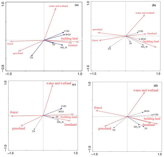
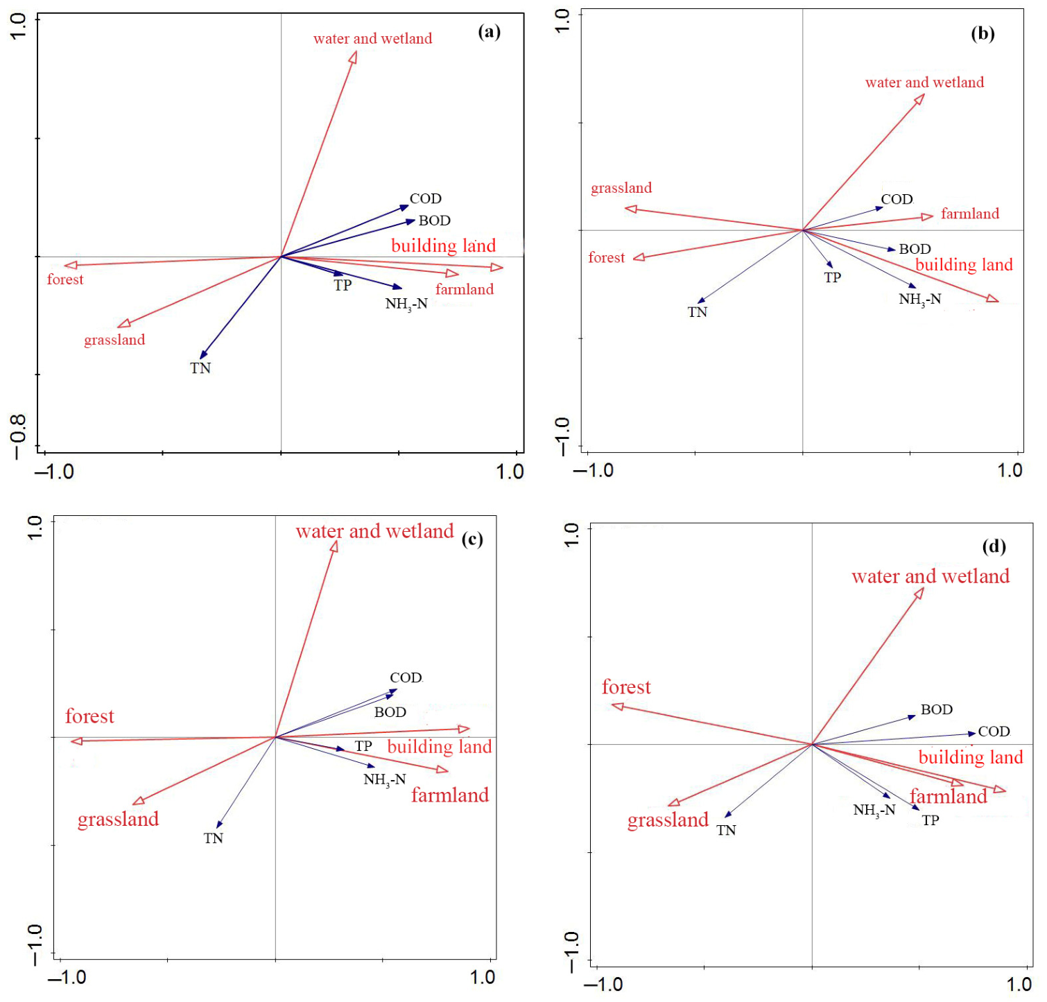
RDA was conducted to explore land use–water quality relationships across multiple buffer scales and subbasins over four periods. Land use explained the most variance in the dry season and the least in the wet season, and it was strongest at the subbasin scale. Sub-basin land use captures basin-scale pollutant generation and hydrological connectivity, whereas riparian buffer zones mainly regulate near-stream retention and filtration. Runoff and basin-scale transport readily mobilize nutrients (TN and TP). In the study area, flood-season flushing and the flat terrain with dense drainage networks further enhance basin-scale pollutant conveyance, whereas narrow, fragmented, or sparsely vegetated riparian buffers have limited retention capacity. Thus, sub-basin land use explains more variance, reflecting the dominance of watershed-scale source and transport processes over near-stream attenuation [20]. The first two axes explained 91% of total variance, supporting the reliability of RDA results. RDA biplots (Figure 3) showed consistent directional responses across scales. Farmland and built-up land were negatively correlated with overall water quality, while forest and grassland were positively correlated (and negatively correlated with pollutant parameters). Notably, farmland and built-up land were not positively associated with TN in this study. These results align with previous studies in the upper Changjiang River basin [12]. In the present study, farmland and built-up land did not contribute positively to TN. Forest ratios > 70% could result in low AN concentrations in water, which originated mainly from agricultural activities (arable land and grassland) [21]. The proportion of farmland and built-up land positively correlated with COD_Mn, BOD, TP, and AN [5]. Farmland in the HRB hosted most human agricultural activities (fertilizer and pesticide use, etc.), making it the primary source of non-point pollution. Built-up land (residential areas, impermeable surfaces, industrial parks, etc.) is highly susceptible to mixed pollution, which worsens water quality. Water pollution varied across residential areas, with AN and TP as the most affected water quality parameters; farmland acted as a sink for TP, AN, and COD_Mn loads [22]. Urban stress strongly influenced water quality; rural and urban parts of the river showed good and medium water quality, respectively [23]. TN concentrations positively correlated with forest and grassland area percentages, but these area percentages negatively correlated with other parameters. Grassland and forest, along with their soil conservation and water storage capabilities, were considered to reduce contaminants in runoff and improve water quality through soil retention and plant root uptake [24,25]. However, TN exhibited a significant positive correlation with the proportion of grassland and forest areas at the spatial scale. TN concentrations in surface waters across China varied significantly by region, mainly influenced by regional background, altitude, human activities, and atmospheric nitrogen deposition. Nitrate sources in Northern China surface waters varied seasonally, with soil organic nitrogen dominating in the flood season (62.81%). By comparison, soil and manure/sanitary sewerage contributed the most during the normal season (48.85% and 21.96%, respectively). In the dry season, household sewage was the primary source (68.03%) [26]. TN concentrations were higher in forest and grassland areas, possibly because organic manure and human activities contributed more. The northwestern region in the HRB is an agriculture-pastoral-forest ecotone, where livestock manure from animal husbandry was a critical source of TN. Water quality was much worse in the plains than in the mountains. Land-use patterns, especially in the 8000 m buffer zone, significantly influenced water-quality changes during dry and wet seasons [27]. The proportion of water and wetland area was negatively correlated with TN concentrations and positively correlated with BOD and COD_Mn concentrations. Forest decline and agricultural activities were significantly correlated with water quality parameters; urban land-use activities such as manufacturing and residential use significantly influenced water quality by altering hydrological processes. Across the four buffer scales (500–5000 m) and the subbasin scale, the directional responses of water quality to land use were broadly consistent; however, the explanatory power of land use generally increased with spatial scale and was strongest at the subbasin scale, indicating that catchment-scale land-use aggregation captures the dominant land-use–water-quality coupling better than the local riparian buffers alone [27]. RDA reveals correlational relationships, not causal mechanisms. Distinguishing the direct and indirect pathways through which land use affects water quality (e.g., via hydrological connectivity, nutrient loading, or in-stream processes) would require structural equation modeling or mediation analysis, which is beyond the scope of this study and is identified as a future research direction.

Figure 3. RDA biplots of land use (red arrows) and water quality parameters (blue arrows) at the subbasin scale: annual (a), wet (b), normal (c), and dry (d) seasons.

3.3.2. Source Apportionment Using PCA-APCS-MLR

PCA was performed after data normalization. KMO (>0.75) and Bartlett’s test (k < 0.001) confirmed PCA suitability. The loadings of ten parameters on varimax-rotated factors were provided in Figure S4. We extracted the first three factors with eigenvalues > 1, which explained 68.1% of the total variance. Several studies reported that cumulative variance above 55% suggested the feasibility of source apportionment with the PCA-APCS-MLR method [12]. Factor 1 (AF1) had strong loadings (0.88, 0.88 and 0.82) on COD_Mn, COD, and BOD; moderate positive loadings (0.545 and 0.66) on TP and fluoride; and a weak positive loading (0.33) on AN, explaining 32.1% of the total variance. High organic matter and nutrient concentrations were likely associated with high emissions from domestic and industrial wastewater [28]. A strong correlation between fluorine-containing rock and F⁻ occurred in North China. The region studied showed high fluoride concentrations in groundwater. Most fluoride in surface water came from anthropogenic sources and natural weathering processes, including phosphate production and coal-fired power generation. Using sewage sludge, phosphate fertilizer, herbicides, and pesticides in agricultural practices could also increase fluoride in river water [29]. AF1 was associated with domestic and industrial wastewater. Factor 2 (AF2, 18.7% of total variance) presented strong positive loading (0.87) on DO, and weak positive loadings (0.45 and 0.36) on TN and pH, and yet strong negative loading (−0.82) on T. It should be noted that, although the loading of F⁻ on AF1 was moderate, fluoride can also originate from natural fluoride-bearing rocks that are widespread in North China; the co-occurrence of F⁻ with organic indicators in AF1 therefore reflects a mixture of anthropogenic effluent (e.g., phosphate production, coal-fired power generation, and sewage sludge application) and natural weathering signals, and the interpretation of AF1 should be made with this mixed origin in mind [29].

AF2 could reflect meteorological and hydrological conditions as environmental driving factors. Water temperature varies by season, suggesting that AF2 may reflect seasonal influence. Oxygen solubility in water decreases as temperature increases. N accumulation in water also increases with high atmospheric deposition during the flood season. Factor 3 (AF3) had moderate positive loadings (0.66, 0.68, and 0.72) on TP, TN, and AN and a moderate negative loading (−0.52) on pH, explaining 17.3% of the total variance. TN, AN, and TP may originate from multiple sources, including animal waste and fertilizer [26]. Rural and agricultural sources contributed most to AN and TP because AN, TP, and livestock density were positively correlated. Therefore, this factor can be considered a non-point source of pollution. Given the strong inverse relationship between water temperature and dissolved oxygen solubility, the loading pattern of AF2 (positive DO, TN, and pH with negative T) is likely dominated by seasonal and hydrological co-variation rather than by a distinct pollution source; AF2 should therefore be interpreted as a combined meteorological–hydrological condition, and the grouping of these parameters should not be over-interpreted as evidence of a specific pollutant discharge.

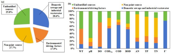
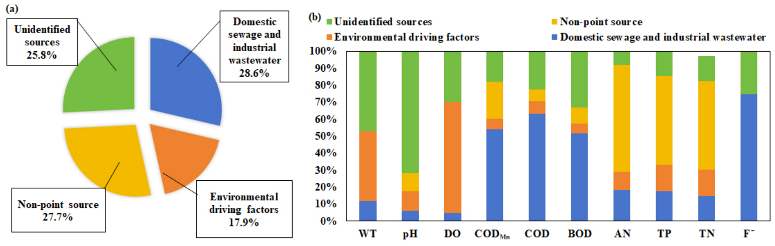
Based on the source-identification results, we calculated the contributions of various sources or factors to water-quality parameters in the HRB using the APCS-MLR model (Figure 4a,b). The results showed that domestic and industrial wastewater (AF1), represented by COD_Mn (65%), COD (66%), and BOD (63%), respectively, accounted for 28.6% of total pollution sources. Meteorological and hydrological conditions (AF2), represented by DO (60%), TN (21%), and TP (12%), accounted for 17.9% of total pollution sources. Non-point pollution sources (AF3) represented by AN (39%), TP (31%), and TN (31%), respectively, accounted for 27.7% of total pollution sources. The contribution rate for unidentified sources in the HRB was estimated at 25.8%. Water pollutants could originate from various sources. For example, TN, TP, and COD may originate from aquaculture wastewater. Some mixed sources could not be separated, resulting in high contributions from unidentified sources in the HRB.

Figure 4. Mean contributions for various sources (a) and contributions to individual parameters (b) using APCS-MLR.

3.3.3. Source Apportionment Based on PMF

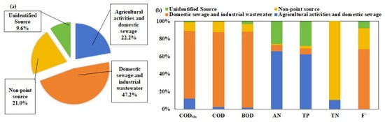
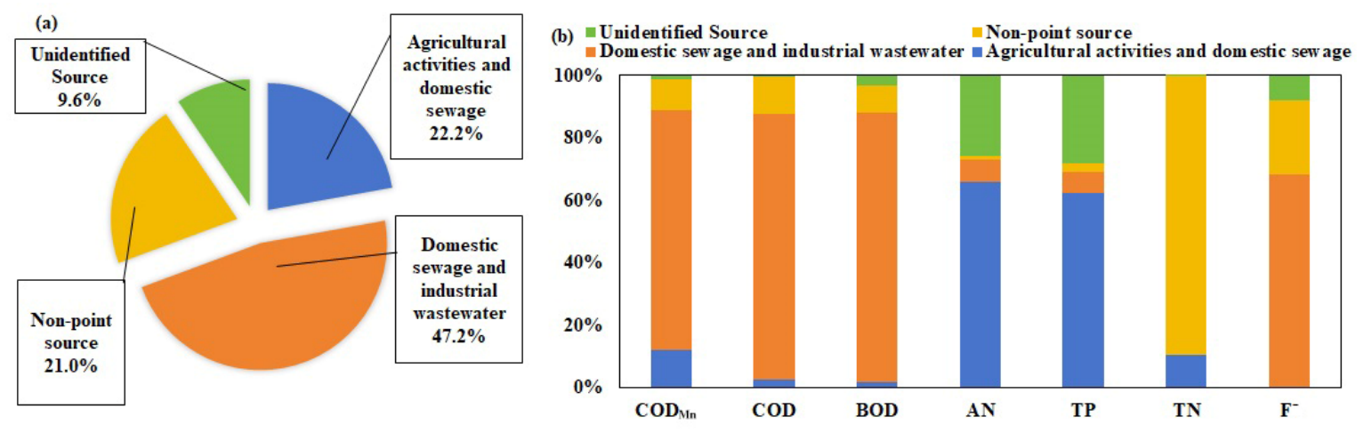
The PMF model was applied to identify potential pollution sources for key water quality parameters (COD_Mn, COD, BOD, AN, TP, TN, and F⁻) in the HRB (Figure 5). Three environmental driving factors or potential sources (PF1–PF3) were identified. Factor 1 (PF1) accounted for 22.2% of total pollution and was characterized by strong loadings of AN and TP. These patterns likely reflect agricultural activities and domestic sewage discharge. TP mainly originates from rural domestic sources, while AN is primarily associated with cropland runoff in the Baiyangdian Basin, a subbasin of the Haihe River Basin [5]. Spatially, AN and TP correlated positively with the areal proportions of construction land and farmland within the catchment. Non-point source pollution from agricultural activities and scattered domestic sewage represented the dominant sources of AN and TP in the HRB, contributing 65.9% and 62.5%, respectively.

Figure 5. Mean contributions for various sources (a) and different parameters using PMF (b).

Factor 2 (PF2) accounted for 47.2% of total pollution and exhibited high loadings of COD_Mn, COD, BOD, and F⁻, indicating organic pollution. Anthropogenic activities, particularly domestic sewage and industrial wastewater, were identified as major sources of these contaminants. Fluoride mainly derives from industrial effluents. PF2 was therefore identified as a mixed source comprising domestic sewage, industrial wastewater, and livestock and poultry breeding [5]. This mixed source dominated BOD, COD, COD_Mn, and F⁻, contributing 76.8%, 85.2%, 86.1%, and 68.2%, respectively. Factor 3 (PF3) explained 21.0% of total pollution and was distinguished by a high TN loading. TN sources are diverse and complex. Average NO₃-N concentrations are higher in the dry season than in the normal and wet seasons, with no significant spatial variation in NO₃-N during the wet season. In the wet season, nitrate in surface water is primarily from non-point sources, with soil organic nitrogen contributing 62.8%. Domestic sewage represents the dominant source in the dry season, accounting for 68.0% of surface-water nitrate. During the normal season, soil organic nitrogen and manure/domestic sewage contribute 48.9% and 22.0% of surface-water nitrate, respectively [26]. The percentage of grassland area in the northwestern HRB was positively correlated with TN, indicating that agricultural and pastoral areas also serve as important TN sources, consistent with previous findings [24]. Accordingly, PF3 was identified as non-point source pollution from agricultural and pastoral activities, which contributed 89.5% of TN. Unrecognized sources contributed 0.2% (TN) to 28.3% (TP) of various surface water quality parameters in the HRB, averaging 9.6%.

3.3.4. Model Fit and Comparison

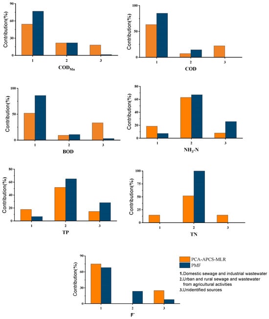
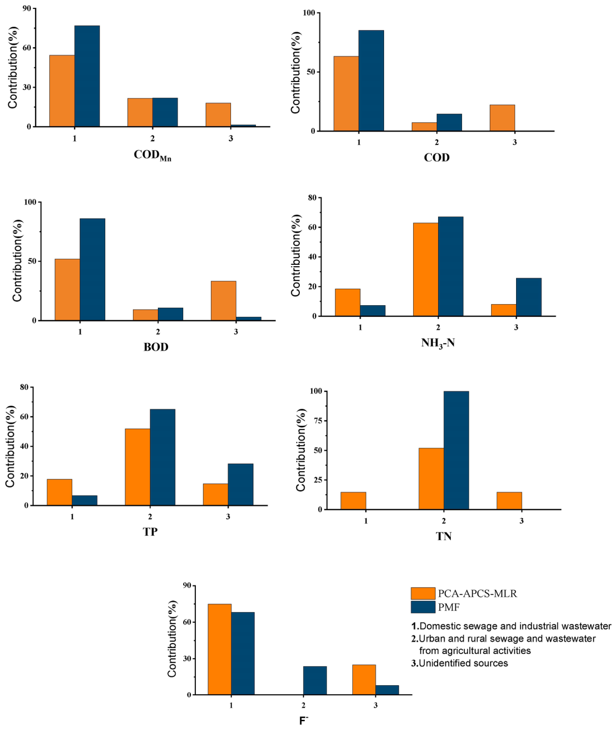
Both the APCS-MLR and PMF models identified three major pollution sources, demonstrating general consistency in source characterization. However, the PCA-APCS-MLR model attributed water quality parameters (WT, pH, and DO) to atmospheric dry and wet deposition. In contrast, the PMF model separately classified TN as an agricultural and pastoral non-point source. A qualitative comparison of contribution rates for the various factors identified by the APCS-MLR and PMF models was shown in Figure 6. Overall, the APCS-MLR model tended to underestimate COD_Mn, COD, and BOD concentrations in AF1. By contrast, the PMF model overestimated TP and TN concentrations in PF2. The PMF model’s relative contribution from unidentified sources (9.6%) was notably lower than the APCS-MLR model (25.8%). The two models differ in input variables, preprocessing, and algorithmic constraints. APCS-MLR applied all 10 normalized parameters, whereas PMF applied seven key parameters with uncertainty weighting. Consequently, the “unidentified” category in APCS-MLR includes variance not captured by the four principal components and residual variance from the regression.

Figure 6. Qualitative comparison of source apportionment using the PCA-APCS-MLR and PMF models.

In contrast, PMF allocates a smaller unexplained fraction to the seven species explicitly included in the factorization. The PMF model accounts for uncertainties in method detection limits, pollutant concentrations, and other external factors, yielding a smaller model error for the selected parameters. The large differences in the estimated source contributions between the two models (e.g., domestic and industrial wastewater: 28.6% vs. 47.2%; unidentified sources: 25.8% vs. 9.6%) arise from several methodological differences: (i) APCS-MLR was applied to the full set of normalized parameters with four extracted components, whereas PMF was run on seven key parameters (COD_Mn, COD, BOD, AN, TP, TN, and F⁻) with three factors; (ii) APCS-MLR partitions variance through regression of the measured concentrations on absolute principal component scores, whereas PMF solves a weighted least-squares factorization that explicitly propagates measurement uncertainty; and (iii) the two models impose different constraints on the source profiles and residual handling. Consequently, the two models allocate different proportions of the total variance to the unidentified category, which does not necessarily indicate that one model is correct and the other is not, but rather reflects their different mathematical structures and input configurations. The PMF solution is more robust here because it formally incorporates measurement uncertainty [10,12]; however, external validation against independent data (e.g., local pollution census and sewage discharge statistics) is still required to confirm individual source attribution and is listed as a future task.

The performance of the two receptor models (APCS-MLR and PMF) for source identification and apportionment was further compared using coefficients of determination (R²). For the APCS-MLR model, R² values ranged from 0.44 to 0.80, with a mean of 0.68, indicating generally good model fit. The pH (0.46) and F⁻ (0.44) had relatively low R² values, likely because these parameters vary widely. An R² value greater than 0.50 suggests satisfactory agreement between measured and predicted values, supporting the reliability of APCS-MLR source apportionment results [12]. For the PMF model, the coefficient of determination ranged from 0.38 to 0.91, with a mean R² of 0.73. The goodness of fit for individual parameters followed the order: TN (0.91) > AN (0.83) > COD_Mn (0.72) > BOD (0.71) > COD (0.66) > TP (0.65) > F⁻ (0.62). The PMF model’s mean R² (0.73) was higher than that of the APCS-MLR model (0.68), indicating that PMF-based source apportionment provides more reliable, robust fits. In addition to R², we evaluated the robustness of the PMF solution by assessing objective-function convergence and factor-profile stability across multiple runs with different random seeds, and by examining residuals of the modeled parameters, following standard diagnostic practice [12].

This study analyzes a two-year dataset (2021–2022). However, it was collected at monthly resolution across 98 sites and covers two complete annual hydrological cycles; it is too short to capture long-term trends and inter-annual variability in HRB water quality, and longer-term monitoring is required to confirm the temporal conclusions. The 98 sampling sites were unevenly distributed across the three river systems, and the study did not conduct a formal spatial representativeness assessment (e.g., variogram or kriging analysis), so interpret the spatial patterns with caution. The monitoring program did not include direct biological parameters (microbial indicators, phytoplankton and cyanobacteria, and bioindicator organisms) or hydro morphological parameters (flow, water level, riverbed and bank structure, and river continuity); BOD was the only biological-related indicator used. Fourth, the source apportionment results of the APCS-MLR and PMF models differ considerably, and the attribution of individual sources has not been independently validated against local pollution census or sewage discharge statistics; moreover, the RDA results describe correlations rather than causal relationships, and no structural equation modeling was performed to separate direct from indirect effects. Although PMF explicitly propagates measurement uncertainty, it has not fully quantified the overall uncertainty associated with monitoring, data processing, modeling, and source interpretation. These limitations set priorities for future research, including longer, more spatially representative monitoring; incorporating biological and hydro morphological indicators; and validating source attribution with independent emission inventories.

3.4. Sustainable Control Strategies

Numerous water pollution prevention and control policies have been developed to mitigate water pollution in the HRB. Establishing an efficient, cost-effective water quality monitoring network is critical to evaluating the effectiveness of water pollution prevention action plans, identifying potential pollution sources, and prioritizing sampling sites. In some cases, routine monitoring programs fail to reflect water quality in water bodies accurately. Local authorities still struggle to create a systematic framework for managing the aquatic environment. Sampling sites should integrate with data on anthropogenic activities. Combining land-use mapping with an assessment of potential pollution risks across the basin can identify optimal sampling sites. Water pollution in the HRB is more severe in areas dominated by farmland and construction land than in other land-use types. The greater the extent and spatial connectivity of these land use categories, the more severe the associated water pollution tends to be. Therefore, optimizing land use patterns in the HRB is essential to reduce the environmental impacts of pollution-source landscapes.

Nitrogen is an essential input for agricultural food production. However, excessive nitrogen inputs across many regions worldwide have triggered widespread water pollution, and controlling nitrogen levels within river basins has become a core objective of most water pollution abatement policies [30]. Anthropogenic reactive nitrogen loads have increased nearly tenfold, leading to the hazardous accumulation of unused reactive nitrogen [31]. Peak TN concentration in the HRB occurred during the non-flood season, while maximum TN concentration in the Yellow River and the Yangtze River basins occurred during the flood season. These differences suggest distinct nitrogen pollution sources among these basins. Further research is urgently needed to better understand nitrogen sources and the distribution of nitrogen speciation in the HRB. Understanding how elevated TN concentrations affect water quality is critical for developing basin-scale management strategies and policies to mitigate nitrogen pollution from agricultural activities, fertilizer production, and sewage treatment facilities within the HRB. Sources of TP and AN in the HRB were largely homogeneous and primarily derived from cultivated land, underscoring the importance of implementing nutrient-loss control measures through optimized cultivation practices. These findings also highlight the need for long-term monitoring to evaluate the effectiveness of relevant management interventions.

In recent years, water pollutant loads in rural areas have become a serious challenge. Water pollution control measures should prioritize reducing pollution from livestock, poultry breeding, and agricultural planting. Rural domestic sewage treatment facilities in China remain insufficient, and their treatment efficiency requires further improvement [3]. Strengthening domestic pollution control requires upgrading pipe networks to collect scattered domestic sewage more effectively. HRB should expand and improve rural domestic sewage treatment facilities to support improvements in water quality.

Based on the source apportionment results, the following differentiated and operational management measures are recommended for the HRB. (1) For TN, which is the primary pollutant and peaks in the mountainous areas and during the non-flood season, monitoring and control efforts should be prioritized in the agro-pastoral ecotone of the northwestern HRB during the non-flood season, emphasizing livestock manure management, the collection of scattered rural domestic sewage, and the control of both nitrate and ammonium (including organic nitrogen) forms; targeted monitoring sections should be established in the mountain-to-plain transition zone and in the rivers discharging into the Bohai Sea. (2) For AN and TP, which are predominantly associated with cultivated land and non-point sources, nutrient-loss control should be implemented through optimized fertilization, conservation tillage, buffer strips, and wetland restoration in the South HR and the plain areas. (3) For the organic indicators (COD_Mn, COD, and BOD), which dominate in the plains and estuaries and are linked to domestic and industrial wastewater, priority should be given to upgrading rural and urban sewage collection networks and to regulating industrial point-source discharges in the Beijing–Tianjin–Hebei region. (4) A risk-based monitoring network should integrate land-use mapping with pollution-source inventories to identify priority control units and to optimize the spatial allocation of monitoring sections and the cost-effectiveness of the monitoring program.

4. Conclusions

Multivariate statistical techniques were employed to analyze spatial and seasonal variations in water quality and to investigate how land-use patterns influence water-quality parameters. PCA identified possible pollution sources and environmental factors in the HRB, and APCS-MLR and PMF calculated their relevant contributions. The conclusions were summarized as follows:

WQI classified water quality in most regions of the HRB as “good”, but TN remained a key concern. TN was the primary pollutant in surface water, exceeding Grade III of the national environmental quality standards and thus requiring primary attention. Water quality in the HRB was better during the flood season than the non-flood season. Nitrogen pollution ranked as mountain areas > plain areas > estuaries, but concentrations of AN, BOD, COD_Mn, and COD ranked as estuaries > plain areas > mountain areas. Water quality in the Luanhe River system was better than in the North Haihe River and South Haihe River systems. Grassland and forest negatively correlated with water-quality parameters. Construction land and farmland adversely affected water quality but did not dominate TN enrichment in the HRB. The APCS-MLR and PMF models successfully apportioned the pollution contributions: domestic and industrial wastewater (28.6% and 47.2%), non-point sources of pollution (27.7% and 22.2%), meteorological and hydrological conditions as environmental driving factors (17.9% and 21.0%), and unidentified sources (25.8% and 9.6%) in the HRB. These findings support the identification of key pollution sources and development of targeted water quality protection strategies in the HRB. Taken together, these results indicate that water quality management in the HRB should be organized around two contrasting pollution regimes: nitrogen-dominated pollution from diffuse rural and pastoral sources in the mountainous areas during the non-flood season, and organic- and nutrient-dominated pollution from agricultural and urban sources in the plains and estuaries during the flood season. Accordingly, implement differentiated strategies, including season- and region-specific TN control in the mountain agro-pastoral ecotone and integrated nutrient-loss and organic-pollution control in the cultivated plains and estuary zones.

References

- Xiong, W.G.; Peng, J.Y.; Li, X.G.; Guo, C.C.; Yang, K.; Wang, W.H.; Lu, X.B.; Lei, K. Spatial-temporal variations and driving factors analysis of total nitrogen concentration in the Haihe River Basin from 2018 to 2022. Environ. Sci. 2025, 46, 184–192. [Google Scholar] [CrossRef] [Scilit] [PubMed]
- Chundu, M.L.; Banda, K.; Sichingabula, H.M.; Nyambe, I.A. Assessing land-use/land-cover influence on surface water quality using a weighted inverse distance function in Bangweulu sub-catchment area, Zambia. Phys. Chem. Earth Parts A/B/C 2025, 137, 103813. [Google Scholar] [CrossRef] [Scilit]
- Cheng, P.; Jin, Q.; Jiang, H.; Hua, M.; Ye, Z. Efficiency assessment of rural domestic sewage treatment facilities by a slacked-based DEA model. J. Clean. Prod. 2020, 267, 122111. [Google Scholar] [CrossRef] [Scilit]
- Umwali, E.D.; Kurban, A.; Isabwe, A.; Mind’je, R.; Azadi, H.; Guo, Z.; Udahogora, M.; Nyirarwasa, A.; Umuhoza, J.; Nzabarinda, V.; et al. Spatio-seasonal variation of water quality influenced by land use and land cover in Lake Muhazi. Sci. Rep. 2021, 11, 17376. [Google Scholar] [CrossRef] [Scilit] [PubMed]
- Hao, C.; Chao, S.; Deng, Y.; Quan, W.; Ying, X.; Yang, X.; Peng, Z. Temporal and Spatial Distribution Characteristics and Source Analysis of Nitrogen in the Yellow River Basin in Qinghai Province. Res. Environ. Sci. 2023, 36, 325–333. [Google Scholar]
- Tao, Y.; Liu, J.; Guan, X.; Chen, H.; Ren, X.; Wang, S.; Ji, M. Estimation of potential agricultural non-point source pollution for Baiyangdian Basin, China, under different environment protection policies. PLoS ONE 2020, 15, e0239006. [Google Scholar] [CrossRef] [Scilit] [PubMed]
- Rodriguez, K.; Arumi, J.L.; Delgado, V. Impact of Regulation on the Water Quality of a Mediterranean River: The Case of the Biobío River. Sustainability 2025, 17, 9997. [Google Scholar] [CrossRef] [Scilit]
- Wei, Q.; Sun, C.; Wu, G.; Pan, L. Haihe River discharge to Bohai Bay, North China: Trends, climate, and human activities. Hydrol. Res. 2017, 48, 1058–1070. [Google Scholar] [CrossRef] [Scilit]
- Wu, G.H.; Ye, D.; Luo, W. Water quality analysis and source apportionment in estuaries along the coast of the Bohai Sea, North China. J. Oceanol. Limnol. 2025, 43, 73–89. [Google Scholar] [CrossRef] [Scilit]
- GB3838-2002; Environmental Quality Standards for Surface Water. China Environmental Science Press: Beijing, China, 2002.
- Haji Gholizadeh, M.; Melesse, A.M.; Reddi, L. Water quality assessment and apportionment of pollution sources using APCS-MLR and PMF receptor modeling techniques in three major rivers of South Florida. Sci. Total Environ. 2016, 566–567, 1552–1567. [Google Scholar] [CrossRef] [Scilit] [PubMed]
- Zhang, H.; Li, H.; Gao, D.; Yu, H. Source identification of surface water pollution using multivariate statistics combined with physicochemical and socioeconomic parameters. Sci. Total Environ. 2022, 806, 151274. [Google Scholar] [CrossRef] [Scilit] [PubMed]
- Ren, X.; Zhang, H.; Xie, G.; Hu, Y.; Tian, X.; Gao, D.; Guo, S.; Li, A.; Chen, S. New insights into pollution source analysis using receptor models in the upper Yangtze river basin: Effects of land use on source identification and apportionment. Chemosphere 2023, 334, 138967. [Google Scholar] [CrossRef] [Scilit] [PubMed]
- Andersson, A. Mechanisms for log normal concentration distributions in the environment. Sci. Rep. 2021, 11, 16418. [Google Scholar] [CrossRef] [Scilit] [PubMed]
- Xie, X.; Li, W.; Li, X.; Huo, X.; Ge, M.; Wang, L. Spatiotemporal Characteristics of Total Nitrogen Concentrations in Rivers Entering the Sea of China from 2020 to 2022. Environ. Monit. China 2023, 39, 90–97. [Google Scholar] [CrossRef]
- Qin, Y.; Ma, Y.; Wang, L. Pollution of the total phosphorus in the Yangtze River Basin: Distribution characteristics, source and control strategy. Res. Environ. Sci. 2018, 31, 9–14. [Google Scholar]
- Wu, G.; Li, J.; Luo, W. Spatial distribution, source apportionment, and assessment of marine water quality parameters in the Bohai Sea, China. Mar. Pollut. Bull. 2023, 195, 115526. [Google Scholar] [CrossRef] [Scilit] [PubMed]
- Xu, H.; Zhu, P.B.; Yue, C.; Ping, L.Y.; Ming, H.Y. Characteristics of Water Environment and Spatial-temporal Distribution of Nitrogen and Phosphorus Load in the Yellow River. Environ. Sci. 2021, 42, 5786–5795. [Google Scholar]
- Camara, M.; Jamil, N.R.; Abdullah, A.F.B. Impact of land uses on water quality in Malaysia: A review. Ecol. Process. 2019, 8, 10. [Google Scholar] [CrossRef] [Scilit]
- Xiang, S.; Pang, Y.; Dou, J.S.; Lü, X.J.; Xue, L.Q.; Chu, Z.S. Impact of land use on the water quality of inflow river to Erhai Lake at different temporal and spatial scales. Acta Ecol. Sin. 2018, 38, 876–885. [Google Scholar] [CrossRef] [Scilit]
- Kändler, M.; Blechinger, K.; Seidler, C.; Pavlů, V.; Šanda, M.; Dostál, T.; Krása, J.; Vitvar, T.; Štich, M. Impact of land use on water quality in the upper Nisa catchment in the Czech Republic and in Germany. Sci. Total Environ. 2017, 586, 1316–1325. [Google Scholar] [CrossRef] [Scilit] [PubMed]
- Lu, J.; Cai, H.; Zhang, X.; Fu, Y. Water quality in relation to land use in the Junshan Lake watershed and water quality predictions. Water Supply 2021, 21, 3602–3613. [Google Scholar] [CrossRef] [Scilit]
- Parween, S.; Siddique, N.A.; Mahammad Diganta, M.T.; Olbert, A.I.; Uddin, M.G. Assessment of urban river water quality using modified NSF water quality index model at Siliguri city, West Bengal, India. Environ. Sustain. Indic. 2022, 16, 100202. [Google Scholar] [CrossRef] [Scilit]
- Ren, X.; Yang, C.; Zhao, B.; Xiao, J.; Gao, D.; Zhang, H. Water quality assessment and pollution source apportionment using multivariate statistical and PMF receptor modeling techniques in a sub-watershed of the upper Yangtze River, Southwest China. Environ. Geochem. Health 2023, 45, 6869–6887. [Google Scholar] [CrossRef] [Scilit] [PubMed]
- Ma, C.; Sun, W.; Yang, Z.; Wang, J.; Zhou, L. Spatiotemporal variations in land use impacts on river water quality in a mountain-to-plain transitional basin in arid region of northern China. J. Contam. Hydrol. 2025, 271, 104542. [Google Scholar] [CrossRef] [Scilit] [PubMed]
- Zhang, E.-C.; Wang, X.; Xu, J.; Cong, X.; Xu, Z.-H.; Xu, L.i.-R.; Liu, B.-W.; Liang, X.-Q.; Liu, M.-Y. Distribution Characteristics and Source Analysis of Nitrate in Surface Water of the Northern Karst Region: A Case Study of the Wohushan Reservoir Basin. China Environ. Sci. 2025, 45, 4965–4974. [Google Scholar] [CrossRef]
- Zhang, H.; Li, H.; Yu, H.; Cheng, S. Water quality assessment and pollution source apportionment using multi-statistic and APCS-MLR modeling techniques in Min River Basin, China. Environ. Sci. Pollut. Res. 2020, 27, 41987–42000. [Google Scholar] [CrossRef] [Scilit] [PubMed]
- Fuge, R. Fluorine in the environment, a review of its sources and geochemistry. Appl. Geochem. 2019, 100, 393–406. [Google Scholar] [CrossRef] [Scilit]
- Luo, M.; Liu, X.; Legesse, N.; Liu, Y.; Wu, S.; Han, F.X.; Ma, Y. Evaluation of Agricultural Non-point Source Pollution: A Review. Water Air Soil Pollut. 2023, 234, 657. [Google Scholar] [CrossRef] [Scilit]
- Cardinale, B.J. Biodiversity improves water quality through niche partitioning. Nature 2011, 472, 86–89. [Google Scholar] [CrossRef] [Scilit] [PubMed]
- Kanter, D.R.; Bartolini, F.; Kugelberg, S.; Leip, A.; Oenema, O.; Uwizeye, A. Nitrogen pollution policy beyond the farm. Nat. Food 2020, 1, 27–32. [Google Scholar] [CrossRef] [Scilit]
Disclaimer/Publisher’s Note: The statements, opinions and data contained in all publications are solely those of the individual author(s) and contributor(s) and not of MDPI and/or the editor(s). MDPI and/or the editor(s) disclaim responsibility for any injury to people or property resulting from any ideas, methods, instructions or products referred to in the content. |
© 2026 by the authors. Licensee MDPI, Basel, Switzerland. This article is an open access article distributed under the terms and conditions of the Creative Commons Attribution (CC BY) license.