


Abstract
This paper presents a scenario analysis of natural-gas substitution with biomethane in the reheating furnaces of a hot-rolling mill exporting steel to the European Union under the Carbon Border Adjustment Mechanism (CBAM) and the phase-out of free allocation in the EU Emissions Trading System over 2026–2034. The model follows the definitive CBAM methodology: embedded emissions of the exported hot-rolled product include the precursor slab, only direct emissions are priced, and certificates are calculated net of the free allocation adjustment. For the case-study mill the product carries 2.48 t CO2e/t, of which the reheating furnaces contribute 4.9%; replacing 20% of natural gas with certified biomethane lowers embedded emissions by about 1%. The resulting CBAM saving of €1.4–3.2 million per year does not depend on the benchmark and remains below the extra fuel cost of €6.9 million, giving a net present value of −€30.8 million over 2026–2034. Substitution breaks even at biomethane prices of €366–427 per thousand m3 for EUA prices of €65–150/t, lower when only part of the CBAM cost is passed through, and yields no saving under default values or without proof of sustainability compliance. For the exporter, verified emissions data are worth considerably more than fuel switching.
1. Introduction
The steel industry accounts for approximately 7–9% of global greenhouse gas emissions [1,2]. The introduction of the Carbon Border Adjustment Mechanism (CBAM) [3] fundamentally changes the regulatory landscape: from 2026 onward, the carbon intensity of steel products acquires direct financial implications for exporters to the European Union [4,5]. The exposure is particularly acute for Ukraine, which entered the definitive CBAM period as the largest exporter of CBAM-covered goods to the EU by physical volume while its industrial base operates under wartime constraints [6]. In parallel, the gradual phase-out of free allocation under the EU ETS during 2026–2034 (from approximately 97.5% to 0%), established by Directive (EU) 2023/959 [7], increases, together with the CBAM, the regulatory pressure on energy-intensive industries and on exporters to the EU [8,9,10].
At steelmaking enterprises producing and exporting steel products to the European Union, rolling mills equipped with reheating furnaces represent a specific case. Their direct fuel-combustion emissions (Scope 1 according to the Greenhouse Gas Protocol classification [11], a boundary for which the lack of reliable records is a recognized barrier to CBAM compliance in the steel sector [12]) are low, but the CBAM is levied on the embedded emissions of the exported product, which for hot-rolled steel include those of the precursor slab [3,13]. For such a mill the reheating furnaces account for only a small share of the embedded emissions of the product, so fuel switching in the furnaces is a marginal lever whose value depends on the carbon price, the share of the CBAM cost passed through by the importer, the price of certified biomethane and the evidence available for its zero-rating.
The aim of this study is to develop an analytical model for assessing natural-gas substitution with biomethane in the reheating furnaces of a hot-rolling mill and to perform a scenario analysis of the effects of market and regulatory factors (carbon prices, the CBAM free allocation adjustment, biomethane availability and price, cost pass-through and certification) on the embedded emissions of the exported product, the CBAM obligation and the financial performance of fuel substitution.
2. Literature Review
2.1. CBAM and Its Impact on the Steel Industry
Research on the implications of the CBAM for the steel industry has intensified since 2021. Using a system dynamics approach, Zhao et al. [14] demonstrated that the CBAM could reduce Chinese steel exports to the EU by 32% and decrease profits by 58%. Bye et al. [15], based on computable general equilibrium (CGE) modeling, showed that the effects of CBAM implementation and the phase-out of free allowances are heterogeneous and vary significantly across industries. Bellora and Fontagné [16] found that the CBAM is effective in reducing carbon leakage but raises the carbon price in the EU ETS and is expected to cause competitiveness losses in export markets for downstream sectors not covered by the mechanism and for European exporters of high-emitting industries. Clausing et al. [17] showed with plant-level data for aluminum and steel that CBAMs can boost domestic competitiveness and reduce emissions leakage while largely avoiding disproportionate burdens on lower-income countries; their simulations include electricity-related (Scope 2) emissions, which the EU CBAM does not price for iron and steel.
Lu et al. [18] quantitatively assessed the long-term impact of the CBAM on the Chinese steel industry under three scenarios (BAU, DCS, and NES), identifying power sector decarbonization as a critical factor. Tian et al. [19] applied evolutionary game theory to analyze the evolution of production decisions at steel enterprises under the influence of the CBAM. Candan and Küçükakça Meral [20] evaluated the sustainable green steel production performance of EU member states to assess whether carbon-free steel production in Europe is attainable. Sgaravatti [21] analyzed the remaining gaps in carbon pricing for EU energy-intensive industries and estimated that an export rebate of the carbon price, requested by EU exporters, could cost about €4 billion per year for iron and steel and €7 billion overall by 2034. Johnson et al. [22] showed that the development of “green” steel production in the EU could become competitive under ETS and CBAM policies; however, risks of competitiveness losses remain in the absence of sufficient deployment of low-carbon technologies. The combined effect of the EU ETS and the CBAM substantially increases carbon-related costs for steel producers, creating new competitive conditions in the emerging green steel market. Ren et al. [23] demonstrated that the introduction of the CBAM significantly increases export costs for Chinese producers trading with the EU and reduces their competitiveness, with total levies on the affected industries ranging from USD 0.07 to 2.25 billion depending on the scenario.
2.2. Technology and Economics of Natural Gas Substitution with Biomethane
The cost of CO2 abatement for industrial decarbonization technologies varies widely, from economically favorable (negative) values in bioenergy systems [24] to substantially higher values for hydrogen production routes, among which biomass gasification has a lower CO2 abatement cost than renewable electrolysis, the lowest being achieved with CCS [25]. For CO2 capture in industry, the cost of CO2 avoided ranges from about USD 34 to 135/t in iron and steel production and from about USD 38 to 199/t in cement production (2016 prices), depending on the route and capture technology [26]. Guerrero et al. [27] conducted a techno-economic assessment of biomass gasification as an alternative to natural gas and coke in energy-intensive industries and showed that the profitability of such projects increases with the prices of natural gas and CO2 emission credits.
D’Adamo et al. [28] showed that the economic viability of biomethane production (€0.54–0.78/m3) strongly depends on public support mechanisms, particularly biofuel certificates (analogous to Guarantees of Origin, GO, instruments certifying the renewable origin of gas), which provide an additional revenue stream for producers. Liebetrau et al. [29] emphasized that biomethane, as a renewable gas, can substitute natural gas within existing infrastructure and support the decarbonization of hard-to-abate sectors, including the steel industry, while its production cost is estimated at €25–100/MWh. Owing to its physicochemical similarity to natural gas and the possibility of using existing gas networks without major infrastructure upgrades, biomethane is considered a “path of least resistance” for the decarbonization of energy and industrial systems [29,30].
A further development of this concept is the Power-to-Biomethane approach. Lanni et al. [31] demonstrated that the integration of electrolytic hydrogen with biogenic CO2 enables biomethane production at a cost of approximately €97/MWh under an optimal hybrid PV–wind configuration, while also providing effective long-term renewable energy storage and supporting decarbonization of the gas sector.
In the industrial context, Mandova et al. [32] showed that biomass can partially replace fossil carbon in European integrated steel plants (coke making, sintering and blast furnace injection), with a CO2 reduction of about 20% at a CO2 price near €60/t and up to 42% at about €140/t, the cost of biomass supply being the main barrier. Biofuels are considered the most readily available short-term solution for existing facilities, provided that sufficient biomass resources and adequate CO2 price levels are available. The resource base itself remains only partly exploited: residual marine biomass, such as the storm-cast macroalgae and seagrass accumulating along the coast of the Sea of Azov, has been shown to sustain stable methanogenesis in a three-stage bioreactor while yielding a digestate suitable for agricultural use [33]. Achievable yields depend strongly on process configuration: reducing the organic loading rate in a three-stage bioreactor raised the methane yield from 175 to 324 L CH4 per kg of volatile solids added [34]. Despite extensive research on the technological aspects of hot rolling and related metal-forming processes, including deformation parameters, temperature regimes, and energy consumption [35,36,37], the substitution of natural gas with biomethane in reheating furnaces and its effects on thermal regimes, energy efficiency, and carbon emissions remain insufficiently addressed in the scientific literature.
2.3. Green Steel Markets and the Research Gap
Rübbelke et al. [38] showed that the introduction of a European Carbon Border Adjustment Mechanism, combined with rising carbon costs under the EU ETS, may improve the competitiveness of hydrogen-based steelmaking routes such as H2-DRI-EAF, although their economic viability remains strongly dependent on energy prices and regulatory conditions. Vogl et al. [39] analyzed the early commercial deployment phase of low-carbon steelmaking in the EU and demonstrated that, due to insufficient infrastructure, uncertain demand, and high investment risks, such technologies are not competitive without public support. Mechanisms such as carbon contracts for difference (CCfDs) were found to be more effective for initiating primary “green” steel production than demand-side instruments, although they require complementary policies to reduce risks and ensure a fair distribution of costs. Koolen and Vidovic [40] conducted a comparative analysis of emission intensities in the EU steel industry and its major trading partners. Hasanbeigi [41] showed that substantial cross-country differences in emissions are driven by production structure (BF–BOF vs. EAF), fuel mix, and technological efficiency. In this context, decarbonization largely depends on changes in the technological structure of production, which directly affect energy consumption and carbon intensity. Kukhar et al. [42,43] demonstrated that the transition from the outdated IOSP + BF + OHF route to the Midrex + EAF route is associated with a significant increase in electricity consumption (reaching approximately 340 kWh/t for EAF operations), while simultaneously enabling substantial CO2 emission reductions due to improved energy efficiency and the use of direct reduced iron technologies.
The literature review reveals four major research gaps. First, most studies focus on the blast furnace–basic oxygen furnace production route, whereas the downstream rolling stage, whose own direct CO2 emissions per unit of output are low, remains largely unexplored. Second, although the technological parameters of rolling and related processes, including temperature regimes, energy consumption, and deformation conditions, are extensively studied in the literature [35,36,37], they are rarely integrated into carbon regulation models or climate policy impact assessments. Third, the economics of fuel switching at a single production stage of a complex good have not been assessed under the definitive CBAM methodology, which combines precursor emissions, the free allocation adjustment and the surrender obligation of the importer. Fourth, the impact of limited biomethane availability (BM_MAX) as a resource constraint on the choice of decarbonization strategies remains insufficiently investigated. Table 1 summarizes the coverage of the reviewed studies; addressing these gaps constitutes the scientific novelty and primary objective of the present study.
Table 1.
Coverage of the reviewed studies and the research gap addressed in this work.
3. Research Methodology
3.1. Case Study Object: Industrial Case-Study Rolling Mill “HRM”
3.1.1. Production Characteristics
For the subsequent analysis, an anonymized industrial hot-rolling mill designated as “HRM” was selected. The case study is based on actual operational and energy-consumption data obtained from an export-oriented steel enterprise. To preserve commercial confidentiality and comply with information-security requirements, the identity of the enterprise and selected operational parameters were anonymized and partially aggregated. The presented characteristics remain representative of the actual industrial conditions considered in this study. The main production, energy, and environmental parameters of the case study object are presented in Table 2.
Table 2.
Production and energy characteristics of the industrial case-study rolling mill “HRM”.
As shown in Table 2, the analyzed facility is characterized by substantial natural-gas consumption (150 million m3/year) and production output (2.5 million t/year), resulting in a significant level of absolute CO2 emissions. The specific carbon footprint of the rolling stage amounts to 0.1224 t CO2e/t; this figure refers to the reheating furnaces only and is not comparable with route-level intensities, because the embedded emissions of the exported product, including the precursor slab, are 2.48 t CO2e/t (Section 3.2.4).
It should be noted that the values presented in Table 2 originate from real industrial operating conditions. Certain production indicators are reported in aggregated form, and some parameters are rounded to representative industrial ranges in order to prevent reverse identification of the enterprise while preserving the validity of the scenario analysis.
The share of exports to the EU was set at 35% as a representative baseline value for the analyzed industrial case; it is an assumption of the case study, motivated by the orientation of Ukrainian exports of CBAM-covered goods toward the European market [6]. At this export level the exported hot-rolled products fall within the scope of the CBAM, and because their embedded emissions include those of the precursor slab, a CBAM obligation arises from 2026 onwards; its level depends on the phase-out of free allocation, the EUA price and whether verified actual data or default values are declared.
Industrial Data Confidentiality
The study is based on operational data obtained from an industrial hot-rolling facility exporting steel products to the European Union. Due to commercial confidentiality obligations and enterprise information-security requirements, the identity of the facility is not disclosed. Several operational indicators are presented in aggregated or rounded form; however, such modifications do not affect the validity of the calculations, the structure of the analytical model, or the conclusions derived from the scenario analysis.
3.1.2. NG/BM Flow Scheme and CO2 Emission Formation
Figure 1 illustrates the conceptual flow scheme of energy carriers and carbon emission formation within the analyzed rolling mill, which serves as the structural basis of the analytical model for assessing decarbonization effects and CBAM-related payments. Although the scheme is presented in generalized form, its structure reflects the actual configuration of fuel consumption and emission sources observed at the industrial facility used as the case study.
Figure 1.
Conceptual diagram of natural-gas/biomethane flows and CO2 emissions formation in the “HRM” rolling mill: model boundaries, precursor slab and emission sources (Scope 1 and the precursor slab included in the embedded emissions of the product; Scope 2 not priced for steel and excluded from the model). Box colors: blue and orange, supply and distribution of natural gas/biomethane; red, Scope 1 emission sources included in the model and the CBAM declaration; green, Scope 2 (electricity) sources excluded from the model; grey, precursor slab; purple, exported product.
The scheme presents the supply and utilization chain of natural gas or biomethane, highlighting the key fuel consumption points and sources of direct CO2 emissions. Reheating and thermal furnaces constitute the primary and effectively the only significant source of direct emissions (Scope 1) within the analyzed facility.
Process units associated with electricity consumption (in particular rolling stands) generate indirect emissions (Scope 2), whereas upstream emissions related to the fuel supply chain (Scope 3) are not considered in the current version of the model.
Thus, the scheme defines the modeling boundaries and the key emission sources directly used in the development of the analytical decarbonization model. The fuel decision concerns the direct fuel-combustion emissions of the rolling stage (Scope 1); for the CBAM obligation these are combined with the embedded emissions of the precursor slab (Section 3.2.3). Electricity-related emissions (Scope 2) are not priced for steel and enter only the hypothetical variant A4-S2.
3.2. Research Design and Analytical Framework
3.2.1. Research Algorithm
The research methodology is structured as a five-block algorithm, schematically presented in Figure 2, which ensures a consistent transition from input data to final analytical conclusions. The overall logic of the study follows a sequential framework: parameterization → mathematical model → baseline analysis → scenario matrix → synthesis of results. This structure reflects the transformation of initial production and energy parameters into quantitative assessments of decarbonization strategies and CBAM-related impacts. Each block represents a distinct stage of the analysis, forming an integrated methodological framework that links system inputs, model formulation, scenario evaluation, and final interpretation of results.
Figure 2.
Five-block research algorithm of scenario analysis for rolling mill decarbonization (V_GAS, annual natural-gas consumption, m3; P_STEEL, steel production, t; EF_NG, emission factor of natural gas, kg CO2/m3; Q_EXP, export volume, t; SEE_SLAB, embedded emissions of the precursor slab, t CO2e/t; BMK, CBAM benchmark, t CO2e/t; EUA, allowance price, €/t; BM_PRICE, biomethane price, €/thousand m3). Colors and icons only distinguish the five sequential blocks.
The first block (parameterization) defines the initial conditions of the system and includes key production, energy, and export parameters, such as fuel consumption, steel output, emission factors, and export shares. These inputs establish the quantitative basis for subsequent modeling.
The second block represents the mathematical model, which integrates carbon-intensity calculations, fuel substitution effects, and CBAM-related payments within a unified analytical framework. This stage formalizes the relationships among energy use, emissions, and financial performance at the enterprise level.
The third block corresponds to the baseline analysis, where the reference state of the system is evaluated under different regulatory and market assumptions. Particular attention is given to the role of biomethane availability (BM_MAX) as a structural constraint affecting decarbonization potential.
The fourth block introduces the scenario matrix, which combines key drivers such as the carbon price (EUA), fuel substitution levels, biomethane availability and price, cost pass-through, certification of the biomethane and the type of emissions data declared. This allows for systematic exploration of alternative system configurations.
The final block provides the synthesis of results, including the comparison of economic and regulatory outcomes across scenarios, identification of risk zones, and determination of break-even conditions for fuel substitution strategies.
Thus, the proposed algorithm serves as the methodological backbone of the study, linking the conceptual framework with the scenario-based analysis and ensuring the internal consistency of the results. All calculations were performed using industrially derived input data representing actual production conditions, while the facility identity remained anonymized throughout the study. The model was implemented in Microsoft Excel, with every result computed by formula from a single input sheet; all inputs are listed in Table 2 and Section 3.2.4, and a step-by-step worked example of the calculation is shown in Section 3.2.3.
3.2.2. Scenario Matrix and Grouping of Drivers
The scenario matrix constitutes the core element of the research design and is structured as a classification of scenarios based on the dominant driver of variation. This approach represents a factor-based decomposition of the system, enabling the separation of regulatory, technological, market, and qualitative influences within a unified analytical framework.
Accordingly, four analytical groups of scenarios are defined. Group A follows the regulatory trajectory of 2026–2034, combining the phase-out of free allocation through the CBAM factor with the EUA path, and compares actual verified data with default values. Group B reflects technological and resource-related conditions, specifically the level of natural-gas substitution and the availability constraint of biomethane (BM_MAX). Group C comprises price scenarios for the EUA price and the biomethane price (BM_PRICE), together with the cost pass-through. Group D represents the certification and quality of the biomethane, including the absence of proof of compliance with the sustainability criteria and variations in the life-cycle emission factor (EF_BM). The scenario matrix comprises sixteen core scenarios (A1–A4, B1–B4, C1–C4 and D1–D4) and two variants, A4-S2 and B4 + ESG; all are listed once with unique labels in Section 5.1.
Such grouping enables the isolation of the effects of individual drivers while maintaining comparability across scenarios and provides a consistent basis for identifying the conditions under which decarbonization strategies become economically and regulatorily effective.
3.2.3. Mathematical Framework for Assessing CBAM Effects and Natural Gas Substitution
The mathematical framework formalizes the relationship among fuel substitution, carbon intensity, and CBAM-related financial outcomes. The model is structured into five interconnected blocks, consistent with the algorithm presented in Figure 2, and enables scenario-based evaluation of decarbonization strategies under regulatory and market constraints.
The source of each equation is stated with it: the fuel-mix and carbon-intensity relations follow the stationary-combustion approach of the IPCC 2006 Guidelines [44] and the GHG Protocol [11]; the CBAM relations follow Regulation (EU) 2023/956 [3] and Implementing Regulations (EU) 2025/2547 [45] and 2025/2620 [13]; and the availability constraint is the authors’ formulation.
Block 1. Mixed emission factor. The mixed emission factor is defined as a linear combination of natural gas and biomethane, weighted by the substitution share α:
EF_mix(α) = EF_NG × (1 − α) + EF_BM × α
This Equation (1) captures the direct impact of fuel switching on emission intensity at the process level. Two values of the biomethane factor are distinguished. For the CBAM declaration, biomethane combustion CO2 is biogenic and zero-rated when compliance with the sustainability criteria of the Renewable Energy Directive is evidenced; otherwise, biomethane carries the natural-gas factor EF_NG = 2.04 kg CO2/m3 (Section 3.2.4). For the climate-impact assessment, a life-cycle factor EF_BM = 0.36 kg CO2e/m3, about 18% of EF_NG, accounts for upstream processing and for methane losses in digestion, upgrading and digestate storage (Section 3.2.4); its feedstock-related variation (−0.07 to 0.94 kg CO2e/m3) is examined in Group D.
For iron and steel, the CBAM covers carbon dioxide only, so CO2 and CO2e coincide numerically for the CBAM quantities; following the implementing regulations, CO2 is used for the combustion factors of fuels and CO2e for embedded emissions, benchmarks and life-cycle factors.
Block 2. Carbon intensity under biomethane availability constraint. To reflect real market conditions, the substitution volume is constrained by the maximum available biomethane supply (BM_MAX) in Equation (2):
V_BM(α) = MIN(V_GAS × α; BM_MAX)
To ensure that the biomethane-availability constraint propagates into all subsequent calculations, the effective substitution share is defined as the fraction of total gas demand actually covered by biomethane in Equation (3):
α_eff(α) = V_BM(α)/V_GAS = MIN(α; BM_MAX/V_GAS)
The resulting carbon intensity is then obtained directly from the actual natural-gas and biomethane volumes (equivalently, by substituting α_eff for α in EF_mix) in Equation (4):
CF_spec(α) = [EF_NG × (V_GAS − V_BM(α)) + EF_BM × V_BM(α)]/(1000 × P_STEEL)
Block 2 introduces a critical real-world constraint, the limited availability of biomethane, which bounds the achievable substitution level and, consequently, the reduction in carbon intensity. This constraint decouples technical substitution potential from market feasibility. Here, BM_MAX denotes the maximum annual biomethane volume available to the enterprise, accounting jointly for production capacity, market availability and gas-infrastructure constraints. In this formulation BM_MAX enters the carbon-intensity expression explicitly through V_BM: whenever the availability ceiling is binding (V_GAS × α > BM_MAX), the effective substitution α_eff, and therefore CF_spec, is governed by BM_MAX rather than by the nominal substitution share α.
Equation (2) is the authors’ formulation of the supply constraint, and Equations (3) and (4) follow from it with the stationary-combustion approach [44]. The range BM_MAX = 15–90 million m3/year used in the scenarios represents 10–60% of the annual gas demand of the mill and is a plant-level supply scenario rather than an estimate of national potential. For comparison, the technical biomethane potential of Ukraine is estimated at 21.8 billion m3/year, whereas production capacity reached about 41 million m3/year in 2025, with about 111 million m3/year planned by the end of that year [46]. The lower end of the range is therefore consistent with near-term supply, while the upper end presupposes substantial market development.
Blocks 3–5. Embedded emissions, CBAM obligation and net financial effect. Blocks 3–5 translate the carbon intensity of the rolling stage into the CBAM obligation of the exported product and into the financial effect of substitution (Table 3). Because hot-rolled flat products (CN 7208) are complex goods, their specific embedded emissions include those of the precursor slab (CN 7207), in addition to the direct emissions of the rolling stage [3,45]. Only direct emissions are taken into account, since iron and steel are listed in Annex II of Regulation (EU) 2023/956 [3]:
where SEE_SLAB is the embedded emissions of the slab per ton of hot-rolled product and CF_CBAM(α) is the rolling-stage intensity of Equation (4) evaluated with the CBAM emission factor of biomethane (Section 3.2.4). The number of CBAM certificates per ton equals the specific embedded emissions minus the specific embedded free allocation, which, with default CBAM benchmarks, is the product of the CBAM factor of year y, the cross-sectoral correction factor and the CBAM benchmark BMK [13]:
SEE(α) = SEE_SLAB + CF_CBAM(α)
N_y(α) = MAX(0; SEE(α) − CBAM_y × CSCF_y × BMK)
Table 3.
Formulation of the CBAM obligation and net financial effect for the rolling mill case.
The annual obligation attributable to the exporter is N_y × Q_EXP × EUA_y × PT, where PT is the share of the CBAM cost of the importer that is passed through to the exporter in the price; the legal surrender obligation rests with the authorized CBAM declarant in the Union [3]. Provided N_y remains positive, the saving from substitution follows from Equations (5) and (6):
SAVE_y(α) = [SEE(0) − SEE(α)] × Q_EXP × EUA_y × PT
Equation (7) contains neither the benchmark nor the CBAM factor: these determine the level of the total obligation but not the saving obtained by reducing embedded emissions. The net financial effect and the break-even biomethane price are
where FUEL_EXTRA = (BM_PRICE − NG_PRICE)/1000 × V_BM(α) is the additional fuel cost and OPEX the additional operating cost of certification and monitoring (Section 3.2.4). Equation (9) gives the fuel price at which the saving offsets the fuel premium, following the marginal abatement cost approach [24]; the fixed costs of implementation are assessed separately in a discounted cash-flow analysis. A step-by-step worked example of the calculation for 2030 is given in Table 4.
NET_y(α) = SAVE_y(α) − FUEL_EXTRA − OPEX
BM_PRICE* = NG_PRICE + 1000 × SAVE_y(α)/V_BM(α)
Table 4.
Worked example of the CBAM calculation for 2030 (verified actual data; compliant biomethane, α = 20%; EUA = €100/t; PT = 100%).
3.2.4. Regulatory Parameters and Their Dynamics
The regulatory environment is a key driver of decarbonization decisions in the steel industry. In the context of the EU Emissions Trading System (EU ETS) reform, the following two interrelated factors are of particular importance: the gradual phase-out of free emission allowances and the expected increase in carbon prices (EUA).
The reduction in free allowances directly increases the exposure of steel producers to carbon costs, while rising EUA prices amplify the financial impact of residual emissions. Together, these mechanisms create a steadily intensifying regulatory pressure over time, which fundamentally affects the economic feasibility of decarbonization strategies.
Figure 3 illustrates the projected dynamics of free allowances and EUA prices for the period 2026–2034. The share of free allowances declines from approximately 97.5% in 2026 to zero by 2034, reflecting the full phase-out under the revised EU ETS Directive. At the same time, EUA prices are assumed to increase from 65 €/t to 150 €/t CO2e, based on available market forecasts.
Figure 3.
Free-allowance phase-out for CBAM sectors (%, bars) under Article 10a(1a) of Directive 2003/87/EC, applied to imports through Article 31 of Regulation (EU) 2023/956 (CBAM factor falling from 97.5% in 2026 to 0% in 2034), and projected EUA prices (€/t CO2e, line). EUA trajectory: authors’ projection based on market forecasts [47,48,49].
In the CBAM, the same phase-out enters through the CBAM factor of Article 10a(1a) of the EU ETS Directive [7], which scales the free allocation adjustment of imported goods in Equation (6).
The third regulatory parameter is the CBAM benchmark. For hot-rolled flat products of carbon steel produced via the BF/BOF route (CN 7208, route C), Implementing Regulation (EU) 2025/2620 sets a default CBAM benchmark of 1.370 t CO2e/t, which covers the precursor chain, and a process-level benchmark of 0.044 t CO2e/t for the rolling stage alone [13]. Benchmarks for 2026–2030 are based on the EU ETS benchmarks determined by Implementing Regulation (EU) 2026/1412 [50], and no values have been adopted beyond 2030. The scenarios therefore use the official value BMK = 1.370 t CO2e/t. Because the saving from substitution does not depend on the benchmark (Equation (7)), the benchmark affects the total obligation of the exporter but not the substitution decision.
For transparency the free allocation adjustment is computed with this Column B benchmark of the product, which covers the precursor chain. With verified actual data the Annex to Implementing Regulation (EU) 2025/2620 provides a precursor-by-precursor calculation; applied here, with a slab consumption of about 1.04 t per ton of hot-rolled product, it would lower the number of certificates by about 8% in 2026 and 3% in 2030, an effect that vanishes by 2034 as the CBAM factor reaches zero. The saving of Equation (7), and hence every result on substitution, is unaffected.
The precursor slab is assigned embedded emissions of SEE_SLAB = 2.36 t CO2e per ton of hot-rolled product. This value corresponds to the Ukrainian default value for hot-rolled flat products of 2.48 t CO2e/t (direct emissions, BF/BOF route) [51] less the rolling-stage intensity of the case-study mill and is varied between 1.60 and 2.36 t CO2e/t in the sensitivity analysis. As a cross-check, the Ukrainian default for slabs (CN 7207) of 2.40 t CO2e per ton of slab, applied with a yield of about 96%, implies a somewhat higher value of about 2.5 t CO2e per ton of hot-rolled product; this would raise the total obligation but would not change the saving from substitution. With the value of 2.36 t CO2e/t the embedded emissions of the product are 2.48 t CO2e/t, of which the rolling stage contributes 0.122 t CO2e/t, or 4.9%. Where the importer declares default values instead of actual verified data, the declared emissions equal the default value with a mark-up of 10% in 2026, 20% in 2027 and 30% from 2028 [51]; the declared emissions then do not depend on the installation, and fuel substitution yields no CBAM saving.
Iron and steel are listed in Annex II of Regulation (EU) 2023/956, so only direct embedded emissions enter the CBAM obligation; emissions related to purchased electricity (Scope 2) are monitored but not priced [3]. The extended accounting with a scalar Scope 2 + 3 increment (Scenario A4-S2) is therefore retained only as an explicitly hypothetical extension of the CBAM scope and is not used to support the main conclusions.
Biomethane is zero-rated in the CBAM declaration only when compliance with the sustainability and greenhouse gas saving criteria of Directive (EU) 2018/2001 [52] is evidenced through a recognized voluntary scheme [53,54,55], for example an ISCC EU Proof of Sustainability together with a Proof of Compliance for the end user, with a mass-balance chain of custody covering injection into and withdrawal from the gas grid [56]. A Guarantee of Origin alone does not provide this evidence. The CBAM emission factor of biomethane is therefore set to zero when compliance is evidenced and to EF_NG otherwise. For the climate-impact assessment, EF_BM is taken from the typical values for biomethane in Annex VI to Directive (EU) 2018/2001 [52], which include methane losses in digestion, upgrading and digestate storage, converted at a lower heating value of 36 MJ/m3: 10 g CO2e/MJ (0.36 kg CO2e/m3) for biowaste with closed digestate and off-gas combustion in the baseline, and −2 to 26 g CO2e/MJ (−0.07 to 0.94 kg CO2e/m3) for the feedstocks of Scenario D2. Grid-quality biomethane is in principle interchangeable with natural gas [57], so burner replacement is not required; however, for furnaces operating at 1200 °C and above, the permissible deviation of the Wobbe index applied to industrial plants is not sufficient to keep the air-to-gas ratio and the furnace temperature within limits [58], which calls for gas-quality measurement and combustion control where biomethane is supplied physically rather than by mass balance through the grid. These items, together with metering and the update of the monitoring plan, are represented by a capital cost of €2.0 million. Certification under a recognized voluntary scheme requires annual audits and mass-balance administration along the value chain [59]; these, with gas-quality analysis, are represented by an operating cost of €0.15 million per year, a deliberately conservative allowance. Both values are stated assumptions. The pass-through share PT is 100% in the baseline and 25–100% in the sensitivity analysis, and a discount rate of 10% is used in the cash-flow assessment.
3.2.5. Scope of Model Application
The proposed analytical model is designed for gas-dependent thermal units in the steel industry, where the primary source of direct emissions (Scope 1) is the combustion of natural gas in reheating or thermal furnaces. Such facilities include rolling mills with reheating furnaces, heat-treatment units, and other installations with a similar energy consumption structure.
The model allows for partial or full substitution of natural gas with biomethane without significant modification of the technological configuration, which makes it suitable for analyzing short- and medium-term decarbonization strategies. The key assumptions are the dominant contribution of gas consumption to Scope 1 emissions and the existence of market access to biomethane (parameter BM_MAX).
For the CBAM assessment of other products, the embedded emissions of the relevant precursors (SEE_SLAB in the present case) must be supplied as an input, since they are determined upstream of the installation analyzed.
The application of the model to electric steelmaking processes, particularly Electric Arc Furnace (EAF) operations, is limited due to the substantial share of indirect emissions (Scope 2), which are not included in the baseline model configuration. For blast-furnace-route units, such as blast furnace (BF) and basic oxygen furnace (BOF) operations, the model is not applicable, since their emissions are primarily generated by the use of solid fossil fuels (coke and coal), while biomethane is not a direct technological substitute.
Thus, the model is generally applicable within the class of gas-dependent thermal units but requires modification for processes dominated by electricity consumption or solid fossil fuels. The case study analyzed in this work represents one such industrial facility and was selected because of the availability of detailed operational data and its relevance to export-oriented steel production under CBAM regulation.
4. Results
4.1. Baseline Analysis: Impact of BM_MAX
To evaluate the impact of biomethane availability on decarbonization outcomes, a baseline analysis was conducted for different BM_MAX values at a fixed substitution rate (α = 60%, chosen so that biomethane availability BM_MAX is the binding constraint across the analyzed range). This approach makes it possible to isolate the effect of supply-side constraints while maintaining constant technological substitution conditions.
Figure 4 illustrates the variation in carbon intensity (CF_spec) across different levels of biomethane availability. The results demonstrate that the achievable emission reduction is determined not only by the substitution rate, but also critically depends on the maximum available biomethane volume.
Figure 4.
Specific carbon footprint of the rolling stage (CF_spec, life-cycle basis, EF_BM = 0.36 kg CO2e/m3) under different biomethane availability levels (BM_MAX) at α = 60%.
At BM_MAX = 30 million m3, the effective substitution is capped at 20% of V_GAS for any nominal share α of 20% or more. This indicates that under constrained supply conditions, biomethane availability becomes the binding constraint, overriding scenario-specific parameters and limiting the potential for further emission reduction.
As shown in Figure 4, increasing BM_MAX leads to a decrease in carbon intensity (CF_spec) that is proportional to the available volume, because at α = 60% the supply constraint is binding over the whole range. Under highly constrained conditions (BM_MAX = 15 million m3), the achievable substitution remains limited, resulting in CF_spec = 0.112 t CO2e/t, which corresponds to only a modest reduction relative to the baseline.
When BM_MAX increases to 30 million m3, the effective substitution reaches 20% of V_GAS, reducing carbon intensity to 0.1022 t CO2e/t. However, further improvements remain limited, as the substitution ceiling is still binding. This confirms that, within this range, biomethane availability, rather than substitution willingness or scenario configuration, determines the outcome.
A more substantial reduction is observed under expanded availability scenarios. At BM_MAX = 60 million m3, carbon intensity decreases to 0.0821 t CO2e/t, corresponding to a 32.9% reduction. Further expansion to BM_MAX = 90 million m3 enables a reduction to 0.0619 t CO2e/t (−49.4%), indicating that deep decarbonization of the rolling stage becomes feasible only when supply constraints are significantly relaxed.
The detailed numerical results are presented in Table 5, which summarizes the relationship between BM_MAX, effective substitution share, carbon intensity, emission reduction, and additional biomethane consumption.
Table 5.
Impact of biomethane availability (BM_MAX) on effective substitution, carbon intensity, and emission reduction.
As shown in Table 5, the effective substitution share increases proportionally with BM_MAX, from 10% under constrained conditions (15 million m3) to 60% in the expanded scenario (90 million m3). This directly translates into a stepwise reduction in carbon intensity and corresponding emission savings.
At the same time, the results reveal a rapid increase in additional biomethane cost, from €3450 thousand/year to €20,700 thousand/year, indicating a growing resource requirement for deeper decarbonization. This highlights a fundamental trade-off between emission reduction and fuel availability.
The linear relationship reflects the MIN function in Equation (2): with α = 60% the cap is binding throughout, so the effective substitution equals BM_MAX/V_GAS; the unequal spacing of the BM_MAX values in Figure 4 does not indicate a change in slope. On the CBAM basis, where compliant biomethane is zero-rated, the corresponding reductions in the embedded emissions of the product are 0.012–0.073 t CO2e/t, or 0.5–3.0% of 2.48 t CO2e/t.
Overall, both Figure 4 and Table 5 consistently demonstrate that biomethane availability acts as a system-defining constraint. Even at a fixed substitution rate, the achievable decarbonization outcome is primarily determined by supply limitations, which define the boundary between technically feasible and practically achievable emission reduction.
4.2. Group A: Regulatory Trajectory and the CBAM Obligation
Group A follows the regulatory trajectory of 2026–2034 at four points (A1–A4: 2026, 2028, 2030 and 2034), combining the CBAM factor of Article 10a(1a) of the EU ETS Directive, the official CBAM benchmark BMK = 1.370 t CO2e/t and the EUA path of Figure 3. The substitution level is α = 20% with BM_MAX = 30 million m3, and the biomethane is compliant (see Figure 5). Table 6 reports the total CBAM obligation of the exported volume under verified actual data and under default values, together with the saving from substitution.
Figure 5.
Net financial effect of biomethane substitution in 2026–2034 under verified actual data, default values and non-compliant biomethane (α = 20%; BM_MAX = 30 million m3; BM_PRICE = €550/thousand m3).
Table 6.
CBAM obligation of the exported volume and effect of biomethane substitution along the regulatory trajectory (Group A; α = 20%; BM_PRICE = €550/thousand m3; PT = 100%).
The obligation grows from €65.2 million in 2026 to €325.8 million in 2034 as the CBAM factor falls and the EUA price rises; under default values, which carry the mark-up of Implementing Regulation (EU) 2025/2621, it is €14.0–97.3 million per year higher. The saving from substitution grows only with the EUA price, from €1.4 million to €3.2 million, and at no point offsets the additional fuel cost of €6.9 million. The benchmark and the CBAM factor change the total obligation by tens of millions of euros but leave the saving unchanged, which confirms the property of Equation (7). For the exporter, the choice between verified actual data and default values is therefore worth one to two orders of magnitude more than fuel substitution in the reheating furnaces.
A hypothetical extension of the CBAM scope to electricity-related emissions, represented by a scalar increment of 0.1014 t CO2e/t (Scenario A4-S2), would raise the 2034 obligation by €13.3 million but would not change the saving, since substitution does not affect electricity consumption; this variant is therefore not considered further.
4.3. Group B: Substitution Level and Biomethane Availability
Group B varies the substitution level together with biomethane availability (B1: α = 10%, BM_MAX = 15 million m3; B2: 20%, 30; B3: 40%, 60; and B4: 60%, 90) under the 2034 conditions of Group A (EUA = €150/t, CBAM factor 0). The results are shown in Table 7 and Figure 6.
Table 7.
Effect of the substitution level and biomethane availability (Group B; 2034; EUA = €150/t; BM_PRICE = €550/thousand m3; PT = 100%).
Figure 6.
CBAM saving and additional fuel cost for the Group B scenarios (2034; EUA = €150/t; BM_PRICE = €550/thousand m3).
Both the saving and the fuel cost scale linearly with the volume of biomethane, so the net loss grows in proportion to the substitution level; even 90 million m3 reduces the embedded emissions of the product by only 3.0%. Scenario B4 + ESG asks which green premium on the exported steel would close the gap: the break-even premium is €12.6 per ton of exports in B4, or €4.4 per ton of total output, and €8.4 and €2.9 per ton respectively in B3. These are thresholds derived from the model rather than observed market prices.
4.4. Group C: Price Conditions
Group C varies the two prices that determine the result, the EUA price (C1: €60/t; C2: €150/t) and the biomethane price (C3: €400; C4: €750 per thousand m3), at α = 20%. Because the saving per thousand m3 of biomethane equals EF_NG × s_EXP × EUA × PT, Equation (9) reduces to a closed form that depends neither on α nor on BM_MAX:
where s_EXP = Q_EXP/P_STEEL is the export share and EF_NG is expressed in t CO2 per thousand m3. With s_EXP = 0.35 and full pass-through, the break-even price is €366/thousand m3 at EUA = €65/t and €427/thousand m3 at €150/t (Table 8). Conversely, at the baseline biomethane price of €550/thousand m3 substitution breaks even only at an EUA price of €322/t, or €113/t if the entire output were exported. In C1 the saving is €1.29 million and the net effect −€5.62 million per year; in C2 the saving is €3.21 million and the net effect −€3.69 million.
BM_PRICE* = NG_PRICE + EF_NG × s_EXP × EUA × PT
Table 8.
Break-even biomethane price (€/thousand m3) by EUA price and cost pass-through share (Equation (10); s_EXP = 0.35).
Lower pass-through lowers the break-even price: at EUA = €150/t it falls from €427 at full pass-through to €374 at 50% and €347 at 25%. The effect of the biomethane price at EUA = €150/t is shown in Table 9: the net effect turns positive only below €427/thousand m3 (C3: +€0.81 million at €400), whereas C4 (€750) gives a loss of €9.7 million in 2034 and €11.5 million in 2026. A decline in the biomethane price through scale and learning would close the gap: at 3% per year the price falls from €550 to €427 in 8.3 years, i.e., close to the end of the horizon in 2034 (2% and 4% per year: 12.5 and 6.2 years).
Table 9.
Effect of the biomethane price on the net financial effect (α = 20%; EUA = €150/t; PT = 100%).
4.5. Group D: Certification, Data and Biomethane Quality
Group D addresses the conditions under which the saving exists at all. In D1 the biomethane is supplied with a Guarantee of Origin but without evidence of compliance with the sustainability criteria of the Renewable Energy Directive; it then carries the natural-gas emission factor in the CBAM declaration, the saving is zero and the net effect equals the full fuel premium of −€6.9 million per year (−€7.05 million with the certification cost). The same outcome arises whenever default values are declared, since the declared emissions then do not depend on the installation. In D2 the life-cycle factor of the biomethane varies with the feedstock (Table 10); this changes the climate benefit but not the CBAM result, because compliant biomethane is zero-rated irrespective of its life-cycle factor.
Table 10.
Effect of the biomethane life-cycle emission factor (Scenario D2; α = 20%; EUA = €150/t; typical values of Annex VI to Directive (EU) 2018/2001 [52] at 36 MJ/m3).
Scenario D3 combines the favorable conditions: compliant biomethane at €400/thousand m3, verified actual data, EUA = €150/t and full pass-through. It is the only configuration with a positive annual result, +€0.81 million (+€0.66 million after the certification cost). Scenario D4 combines the unfavorable ones, biomethane at €750/thousand m3 and declaration by default values, and yields a loss of €12.9 million per year with no CBAM saving.
4.6. Dynamic Analysis of Decarbonization Trajectories (2026–2034)
Table 11 and Figure 7 show the annual net effect for representative scenarios and the net present value over 2026–2034, which includes the implementation capital cost of €2.0 million, the certification cost of €0.15 million per year and a discount rate of 10%.
Table 11.
Annual net financial effect (thousand €) and net present value of biomethane substitution, 2026–2034 (α = 20%; PT = 100%).
Figure 7.
Annual net financial effect of biomethane substitution in 2026–2034 for representative scenarios (thousand €/year).
The net effect improves only with the EUA price. Under the C3 price the annual effect turns positive in 2032, but the net present value over 2026–2034 remains −€4.8 million because of the early years and the implementation cost; in the other cases it ranges from −€30.8 million to −€65.3 million. Within the study horizon substitution is therefore a cost rather than a source of return, unless certified biomethane is available close to €400/thousand m3 and the EUA price approaches €150/t.
4.7. Sensitivity Analysis and Economic Feasibility Boundaries
Equation (10) makes the feasibility boundary explicit. Figure 8 shows the net effect in 2034 as a function of the biomethane price, crossing zero at €427/thousand m3, and Figure 9 shows the break-even biomethane price as a function of the EUA price for pass-through shares of 25–100%. Because the boundary depends on the export share, the pass-through and the EUA price but not on α or BM_MAX, the substitution level determines the magnitude of the result, not its sign. The export share acts in the same way as the pass-through: the saving scales linearly with the exported tonnage, so a change in the share of exports to the EU from 35% to 25% or 45% changes the saving and the break-even price premium over natural gas of Equation (10) proportionally.
Figure 8.
Net financial effect of biomethane substitution in 2034 as a function of the biomethane price (α = 20%; EUA = €150/t; PT = 100%); break-even at €427/thousand m3.
Figure 9.
Break-even biomethane price as a function of the EUA price for pass-through shares of 25–100% (export share 35%; Equation (10)).
5. Discussion
5.1. Integrated Comparison of All Scenarios
Table 12 lists every case once with a unique label: the sixteen core scenarios A1–D4 and two variants, A4-S2 (hypothetical extension of the CBAM scope to electricity-related emissions) and B4 + ESG (break-even green premium). Group A is evaluated in its respective year and Groups B–D in 2034, the year of the highest carbon price; Figure 10 shows the net effects.
Table 12.
Register of scenarios and their results (thousand €/year).
Figure 10.
Net financial effect of biomethane substitution for all scenarios (thousand €/year; Group A in the respective year, Groups B–D in 2034).
Only two cases yield a positive annual result, C3 and D3, and both require biomethane at €400/thousand m3, below the break-even price of €427/thousand m3 at EUA = €150/t; D3 differs from C3 only by the certification cost. The largest losses arise where the saving disappears (D1, D4) or the fuel premium is large (C4, B4). Across the groups the result is governed by three quantities, namely the biomethane price premium, the EUA price and the share of the CBAM cost borne by the exporter, and by two conditions, certified biomethane and verified actual data, without which the saving is zero. The benchmark, the CBAM factor and BM_MAX change the total obligation or the scale of the result, but not its sign.
5.2. Strategic Recommendations
5.2.1. Strategic Decision Tree
Figure 11 summarizes the decision logic. For an exporter of hot-rolled steel the first question is not whether its direct emissions exceed a benchmark, since the product carries the precursor emissions and the obligation is positive in every year, but whether verified actual data can be declared; without them no reduction at the installation reduces the obligation. The second question is whether biomethane can be procured with evidence of compliance with the sustainability criteria of the Renewable Energy Directive; without it the saving is zero. Only when both conditions hold does the comparison of the offered biomethane price with the break-even price of Equation (10) decide whether substitution adds value.
Figure 11.
Decision tree for a hot-rolling exporter under the CBAM: verified data, certified biomethane and the break-even price of Equation (10). Box colors: orange, starting point; blue, decision nodes; red, priority action when verified data are not declared; grey, no switching or monitoring; green, recommended action (contracting of certified biomethane).
5.2.2. Recommendation Matrix
Table 13 translates the results into recommendations for exporters in different situations.
Table 13.
Recommendation matrix for hot-rolling exporters under the CBAM.
5.2.3. Ranking of Factors Influencing the Net Effect
To rank the factors on a common basis, each parameter was varied between the bounds of a stated plausible range with all other parameters at the 2034 baseline (α = 20%, EUA = €150/t, BM_PRICE = €550/thousand m3, PT = 100%, and s_EXP = 35%), and the parameters were ordered by the resulting swing in the net effect (Table 14).
Table 14.
Ranking of factors by the swing in the net financial effect between the bounds of their plausible ranges (thousand €/year; 2034 baseline).
The biomethane price is the dominant factor and the only one that changes the sign of the result within its plausible range. The substitution level scales the loss without changing its sign, as Equation (10) implies. Certification and verified data act as a switch on the saving. The benchmark and the CBAM factor, which govern the total obligation, have no influence on the substitution decision, and the life-cycle emission factor affects only the climate benefit.
5.3. Interpretation of Results and Study Limitations
5.3.1. Comparison with the Existing Literature
The results are consistent with recent studies on how the CBAM and its design shape the incentives for reducing the carbon footprint of industrial products [60,61,62], and they quantify these incentives for the downstream rolling stage. Because the embedded emissions of hot-rolled steel are dominated by the precursor slab, the CBAM exposure of a rolling mill is substantial from 2026 onwards, but the share of that exposure which the mill can influence through its own fuel choice is small, 4.9% of embedded emissions in the case examined. The incentive for fuel switching at this stage is therefore real but limited, and it is set by the EUA price and the cost pass-through rather than by the benchmark.
Bye et al. [15] indicate that CBAM, in combination with EU ETS mechanisms, is intended to reduce carbon leakage risks by equalizing carbon-related regulatory pressure between internal and external producers. At the same time, recent quantitative studies show that the economic impact of CBAM remains ambiguous: while it may improve EU welfare and alter trade structures, it provides only moderate emission reductions and is accompanied by a redistribution of gains and losses among countries and industrial sectors [62,63]. Furthermore, the CBAM is expected to reduce the export competitiveness of non-EU producers, most sharply for India, Russia and Turkey, while for China part of the losses can be offset by its national emissions trading system [64]. At plant level, the results obtained in this study demonstrate that regulatory pressure alone is insufficient to ensure the economic feasibility of fuel substitution. Under the baseline biomethane price level (BM_PRICE = €550/thousand m3), most scenarios remain financially negative even at EUA = €150/t, whereas a positive effect is achieved only under the combined conditions of stringent climate regulation and reduced biomethane costs.
Because the saving scales with the EUA price, its value to the exporter also depends on how carbon-price risk is managed. Liu et al. [65] show that energy-consuming enterprises can optimize the timing of allowance purchases under price uncertainty, which suggests that hedging the carbon price and switching fuel are complementary rather than alternative instruments.
The conclusion of Mandova et al. [32] that the economics of biomass substitution in integrated steel plants is governed by the carbon price and the cost of biomass supply is also confirmed by the present results for the rolling stage. At the same time, the modeling performed in this study demonstrates a fundamental distinction between technological availability and economic viability of such solutions. Under conditions of BM_MAX = 30 million m3 and BM_PRICE = €550/thousand m3, natural-gas substitution is technically feasible; however, in most scenarios it does not ensure a positive financial outcome without additional regulatory or market-based incentives. This finding is consistent with studies emphasizing the ambiguous economic effects of climate policy and the strong dependence of decarbonization efficiency on market and regulatory parameters [32,63].
D’Adamo et al. [28] emphasize the growing role of certification and verification of low-carbon fuels. The present results make this concrete for the CBAM: zero-rating of biomethane requires evidence of compliance with the sustainability criteria of the Renewable Energy Directive, and a Guarantee of Origin alone does not provide it. Without such evidence, or when default values are declared, the saving from substitution is zero and the net effect equals the full fuel premium.
The results also align with studies focused on the development of H2-DRI-EAF technologies as a strategic decarbonization pathway for the steel industry, which are widely regarded as a key long-term low-carbon route for steel production [22,39]. Unlike hydrogen-based technologies, which require substantial capital investments, infrastructure development, and relatively high hydrogen prices to achieve competitiveness, biomethane substitution scenarios may be implemented within the framework of existing reheating furnace infrastructure. In this context, biomethane substitution may be considered an intermediate or transitional decarbonization stage capable of providing approximately 8–49% reduction in rolling-stage emissions without complete reconstruction of the production cycle.
Thus, the results complement the existing literature by linking a stage-level fuel decision to the product-level CBAM obligation. Unlike studies that address the macro-level effects of the EU ETS and the CBAM, the present analysis shows that at the level of a rolling mill the economic result of fuel switching is determined by the biomethane price premium, the EUA price and the cost pass-through, provided the following two institutional conditions are met: certified biomethane and verified actual data. The benchmark and the CBAM factor shape the total obligation, and hence the competitiveness of the exporter, but not the value of switching fuel.
5.3.2. Study Limitations
The study has several limitations that should be considered when interpreting the scenarios. First, the precursor emissions of the slab are represented by a single value derived from the Ukrainian default for hot-rolled flat products; in practice a verified value from the slab supplier would replace it. Because the saving from substitution does not depend on the precursor value, this affects the total obligation but not the substitution result. Second, the CBAM benchmark and the CBAM factor are those currently adopted; benchmark values beyond 2030 have not been set, and the cross-sectoral correction factor is taken as 1.0. Third, the implementation costs, a capital cost of €2.0 million and a certification cost of €0.15 million per year, are stated assumptions rather than quotations; their inclusion lowers the net present value but does not change the sign of any result.
Fourth, transparent transaction data on green premiums for low-carbon steel remain scarce, so the study reports the break-even premium (€12.6 per ton of exports in B4) instead of assuming a market value. Fifth, production volume, export share and gas consumption are held constant; because the saving is linear in the exported tonnage, a change in the export share changes the result proportionally, but output shocks under wartime conditions are not modeled stochastically. Sixth, the scenario design is deterministic; a probabilistic treatment of EUA and biomethane prices, for example by Monte Carlo simulation, is a natural extension. Finally, the biomethane price is constant within each scenario; a learning-driven decline of 3% per year would bring it to the break-even level by about 2034.
5.4. Scientific Novelty
The elements of scientific novelty of the study are summarized in Table 15.
Table 15.
Elements of scientific novelty of the study and their distinction from existing approaches.
The contribution therefore lies in the explicit link between a stage-level fuel decision and the product-level CBAM obligation, and in the analytical and institutional conditions under which that decision adds value.
6. Conclusions
This study developed an analytical model for evaluating natural-gas substitution with biomethane in the reheating furnaces of a hot-rolling mill exporting to the European Union, under the definitive CBAM methodology and the phase-out of free allocation over 2026–2034. The model links the rolling-stage fuel decision to the embedded emissions of the exported product, including the precursor slab, and to the CBAM obligation net of the free allocation adjustment.
For the case-study mill the exported product carries 2.48 t CO2e/t, of which the reheating furnaces contribute 4.9%. The CBAM obligation of the exported volume rises from €65 million in 2026 to €326 million in 2034 with verified actual data and is €14–97 million per year higher under default values. Exposure to the CBAM is therefore substantial for a rolling mill, but it is dominated by the precursor.
Replacing 20% of natural gas with certified biomethane reduces embedded emissions by about 1% and yields a CBAM saving of €1.4–3.2 million per year, which does not depend on the benchmark or the CBAM factor and remains below the extra fuel cost of €6.9 million at €550/thousand m3. Over 2026–2034 the net present value is −€30.8 million. Only scenarios C3 and D3, with biomethane at €400/thousand m3 and EUA at €150/t, give a positive annual result, and even then, the net present value over the horizon remains negative (−€4.8 million).
The break-even biomethane price follows the closed form of Equation (10) and is independent of the substitution level and of biomethane availability: €366–427/thousand m3 for EUA prices of €65–150/t at full pass-through and lower when only part of the CBAM cost is passed through to the exporter. At the baseline biomethane price substitution would break even only at an EUA price of about €322/t.
Two institutional conditions are decisive. Biomethane must be supplied with evidence of compliance with the sustainability criteria of the Renewable Energy Directive, since a Guarantee of Origin alone does not permit zero-rating, and the importer must declare verified actual data, since under default values no reduction at the installation reduces the obligation. Biomethane availability limits the scale of substitution, and the upper end of the range considered exceeds the current biomethane production capacity of Ukraine.
For a rolling mill exporting hot-rolled steel to the EU, the first priorities under the CBAM are therefore verified emissions data and the carbon intensity of the slab supply. Fuel switching in the reheating furnaces is a secondary lever, economically justified only when certified biomethane is available below the break-even price of Equation (10).
Author Contributions
Writing, original draft preparation, V.B.; writing, review and editing, V.B., V.K., A.Z., P.K.D.M. and A.K. All authors have read and agreed to the published version of the manuscript.
Funding
This research received no external funding. The APC was supported by P.K.D.M.
Institutional Review Board Statement
Not applicable.
Informed Consent Statement
Not applicable.
Data Availability Statement
The data supporting the reported results are contained within the article. The complete scenario model (Microsoft Excel workbook, Microsoft 365) is available from the corresponding author upon reasonable request.
Conflicts of Interest
The authors declare no conflicts of interest.
Abbreviations
The following abbreviations are used in this manuscript:
| A1–A4 | Scenarios of Group A describing the regulatory trajectory 2026–2034 (CBAM factor, EUA price) under verified actual data and default values |
| B1–B4 | Scenarios of Group B describing different levels of natural-gas substitution by biomethane and biomethane availability constraints |
| BAU | Business-as-Usual Scenario (scenario assuming continuation of existing policies without additional decarbonization measures) |
| BF | Blast Furnace |
| BF–BOF | Blast Furnace–Basic Oxygen Furnace steelmaking route |
| BM | Biomethane |
| BMK | CBAM benchmark for the exported product (t CO2e/t); 1.370 t CO2e/t for CN 7208, BF/BOF route |
| BM_MAX | Maximum available biomethane volume (m3/year) |
| BM_PRICE | Biomethane price (€/thousand m3) |
| BOF | Basic Oxygen Furnace |
| C1–C4 | Scenarios of Group C describing EUA and biomethane price conditions and their impact on financial feasibility |
| CBAM | Carbon Border Adjustment Mechanism |
| CBAM_y | CBAM factor of year y, the share of free allocation retained under Article 10a(1a) of Directive 2003/87/EC |
| CCfD | Carbon Contracts for Difference |
| CF_base | Baseline specific carbon footprint of the rolling stage before biomethane substitution (t CO2e/t) |
| CF_spec | Specific carbon footprint of the rolling stage under a given scenario (t CO2e/t) |
| CGE | Computable General Equilibrium |
| CN | Combined Nomenclature product classification used in EU trade and CBAM regulation |
| CO2 | Carbon dioxide |
| CO2e | Carbon dioxide equivalent |
| CSCF | Cross-sectoral correction factor (taken as 1.0) |
| D1–D4 | Scenarios of Group D describing certification of biomethane, the type of emissions data declared and the life-cycle emission factor |
| DCS | Decarbonization Scenario (scenario with accelerated implementation of low-carbon technologies and emission reduction policies) |
| DRI | Direct Reduced Iron |
| EAF | Electric Arc Furnace |
| E_base | Baseline Scope 1 emissions from natural-gas combustion before substitution (t CO2e/year) |
| EF | Emission factor |
| EF_BM | Emission factor of biomethane (kg CO2e/m3) |
| EF_mix | Mixed emission factor of the NG/BM fuel blend after biomethane substitution (kg CO2e/m3) |
| EF_NG | Emission factor of natural gas (kg CO2/m3) |
| ESG | Environmental, Social, and Governance |
| ETS | Emissions Trading System |
| EU | European Union |
| EU ETS | European Union Emissions Trading System |
| EUA | European Union Allowance, i.e., EU carbon allowance price under EU ETS (€/t CO2e) |
| FUEL_EXTRA | Additional fuel cost caused by replacing natural gas with biomethane |
| GHG | Greenhouse Gas |
| GO | Guarantee of Origin, certificate confirming the renewable origin of biomethane or renewable gas |
| HRM | Hot-Rolling Mill, representative enterprise analyzed in the study |
| H2 | Hydrogen |
| H2-DRI-EAF | Hydrogen-based Direct Reduced Iron–Electric Arc Furnace steelmaking route |
| IOSP | Iron Ore Sintering Plant |
| IOSP + BF + OHF | Conventional steelmaking route based on iron ore sintering, blast furnace, and open-hearth furnace |
| IPCC | Intergovernmental Panel on Climate Change |
| ISCC | International Sustainability and Carbon Certification |
| MAX | Maximum function used in model equations |
| Midrex | Direct reduction ironmaking technology used for DRI production |
| MIN | Minimum function used to impose the biomethane availability constraint |
| NES | Net-Zero Emissions Scenario (scenario targeting net-zero greenhouse gas emissions by 2050 through deep industrial and energy transition) |
| NET | Net financial effect of biomethane substitution after CBAM savings, additional fuel costs and OPEX, Equation (8) |
| NG | Natural Gas |
| NG_PRICE | Natural-gas price (€/thousand m3) |
| NPV | Net present value |
| N_y | Number of CBAM certificates per ton of exported product in year y, Equation (6) |
| OHF | Open-Hearth Furnace |
| OPEX | Additional operating expenditure for certification and monitoring (€/year) |
| P_STEEL | Annual steel production volume (t/year) |
| PT | Share of the CBAM cost of the importer passed through to the exporter |
| PV | Photovoltaic energy system |
| Q_EXP | Annual export volume of steel products to the EU (t/year) |
| q_spec | Specific natural-gas consumption per ton of steel (m3/t steel) |
| RED | Renewable Energy Directive (EU) 2018/2001 |
| S0 | Baseline scenario without biomethane substitution |
| SAVE | CBAM saving from substitution (thousand €/year), Equation (7) |
| Scope 1 | Direct greenhouse gas emissions from on-site fuel combustion |
| Scope 2 | Indirect greenhouse gas emissions from purchased electricity |
| Scope 2 + 3 | Combined indirect emissions from electricity consumption and supply-chain processes |
| Scope 3 | Other indirect upstream and supply-chain greenhouse gas emissions |
| SEE | Specific embedded emissions of the exported product, including the precursor (t CO2e/t) |
| SEE_SLAB | Embedded emissions of the precursor slab per ton of hot-rolled product (t CO2e/t) |
| SEFA | Specific embedded free allocation, CBAM_y × CSCF_y × BMK (t CO2e/t) |
| s_EXP | Export share, Q_EXP/P_STEEL |
| USD | United States dollar |
| V_BM | Volume of biomethane consumed (m3/year) |
| V_GAS | Annual natural-gas consumption (m3/year) |
| α | Biomethane substitution share, expressed as a fraction of V_GAS |
References
- Kim, J.; Sovacool, B.K.; Bazilian, M.; Griffiths, S.; Lee, J.; Yang, M.; Lee, J. Decarbonizing the iron and steel industry: A systematic review of sociotechnical systems, technological innovations, and policy options. Energy Res. Soc. Sci. 2022, 89, 102565. [Google Scholar] [CrossRef] [Scilit]
- Rathore, D. Toward green steel: Role of pilot-scale carbon capture and utilization technologies. Energy Sustain. Dev. 2025, 89, 101866. [Google Scholar] [CrossRef] [Scilit]
- European Parliament; Council of the European Union. Regulation (EU) 2023/956 of the European Parliament and of the Council establishing a carbon border adjustment mechanism. Off. J. Eur. Union 2023, L 130, 52–104. [Google Scholar]
- Zhu, J.; Zhao, Y.; Zheng, L. The impact of the EU carbon border adjustment mechanism on China’s exports to the EU. Energies 2024, 17, 509. [Google Scholar] [CrossRef] [Scilit]
- Minten, H.; Hausweiler, J.; Probst, B.; Reinert, C.; Meys, R.; Bardow, A. Embodied emissions of chemicals within the EU Carbon border adjustment mechanism. Nat. Sustain. 2025, 8, 1381–1390. [Google Scholar] [CrossRef] [Scilit]
- Kukhar, V.; Burko, V.; Khliestova, O.; Kara De Maeijer, P.; Korjakins, A. War-Driven Transformation of Stationary Air Pollutant and Greenhouse Gas Emissions in Ukraine: Evidence from Official Statistics and Implications for CBAM and the National Emissions Trading System. Pollutants 2026, 6, 50. [Google Scholar] [CrossRef] [Scilit]
- European Parliament; Council of the European Union. Directive (EU) 2023/959 of the European Parliament and of the Council amending Directive 2003/87/EC establishing a system for greenhouse gas emission allowance trading within the Union and Decision (EU) 2015/1814 concerning the establishment and operation of a market stability reserve for the Union greenhouse gas emission trading system. Off. J. Eur. Union 2023, L 130, 134–202. [Google Scholar]
- Zetterberg, L.; Elkerbout, M. What Lies Ahead for the EU ETS? (NEPP Resultatblad 2/2025). Energiforsk. 2025. Available online: https://energiforsk.se/media/34065/what-lies-ahead-for-the-eu-ets-2025_1.pdf (accessed on 8 September 2026).
- Dobranschi, M.; Nerudová, D.; Solilová, V.; Stadler, K. Carbon border adjustment mechanism challenges and implications: The case of Visegrad countries. Heliyon 2024, 10, e30976. [Google Scholar] [CrossRef] [Scilit] [PubMed]
- Wirdyansyah, D.M. Carbon border adjustment mechanism (CBAM) and its implications for developing economies: A systematic literature review. Indones. J. Energy 2025, 8, 162–176. [Google Scholar] [CrossRef] [Scilit]
- World Resources Institute and World Business Council for Sustainable Development. Greenhouse Gas Protocol. Corporate Accounting and Reporting Standard, Revised ed.; World Resources Institute and World Business Council for Sustainable Development: Washington, DC, USA, 2004; Available online: https://ghgprotocol.org/sites/default/files/standards/ghg-protocol-revised.pdf (accessed on 8 September 2026).
- Malik, S.A.A.; Qureshi, S.; Ijaz, A.; Zulfiqar, M. Monitoring, verification, and trade exposure: Evaluating cross-border adjustment mechanism (CBAM) compliance in Pakistan’s steel sector. Eng. Proc. 2025, 111, 40. [Google Scholar] [CrossRef] [Scilit]
- European Commission. Commission Implementing Regulation (EU) 2025/2620 of 16 December 2025 laying down rules for the application of Regulation (EU) 2023/956 of the European Parliament and of the Council as regards the calculation of the free allocation adjustment to the number of CBAM certificates to be surrendered. Off. J. Eur. Union 2025, L, 2025/2620. Available online: http://data.europa.eu/eli/reg_impl/2025/2620/oj (accessed on 6 October 2026).
- Zhao, L.-T.; Chen, Z.-Y.; Duan, Y.-X.; Qiu, R.-X. How will CBAM affect the decarbonization of steel industry in China? A system dynamics approach. Int. J. Prod. Res. 2024, 62, 6859–6880. [Google Scholar] [CrossRef] [Scilit]
- Bye, B.; Kaushal, K.R.; Storrøsten, H.B. EU’s carbon border adjustment mechanism (CBAM)—Industrial effects. Clim. Policy 2025, 1–13. [Google Scholar] [CrossRef] [Scilit]
- Bellora, C.; Fontagné, L. EU in search of a carbon border adjustment mechanism. Energy Econ. 2023, 123, 106673. [Google Scholar] [CrossRef] [Scilit]
- Clausing, K.A.; Colmer, J.M.; Hsiao, A.; Wolfram, C. The Global Effects of Carbon Border Adjustment Mechanisms (NBER Working Paper No. 33723); National Bureau of Economic Research: Cambridge, MA, USA, 2025. [Google Scholar] [CrossRef] [Scilit]
- Lu, B.; Liu, X.; Hong, J.; Mo, K.; You, J.; Niu, N.; Wang, Z. Quantifying the long-term impact of carbon border adjustment mechanism on Chinese steel industry. iScience 2026, 29, 115089. [Google Scholar] [CrossRef] [Scilit] [PubMed]
- Tian, B.; Pan, C.; Xing, Y.; Gu, Y. Analysis of production decision-making evolution of steel enterprises under carbon border adjustment mechanism. Heliyon 2024, 10, e33382. [Google Scholar] [CrossRef] [Scilit] [PubMed]
- Candan, G.; Küçükakça Meral, Z. Is a carbon-free Europe possible? Evaluation of sustainable green steel production performance in EU member states. Appl. Energy 2026, 409, 127431. [Google Scholar] [CrossRef] [Scilit]
- Sgaravatti, G. How to Fill the Remaining Gaps in Pricing the Emissions of the EU’s Energy-Intensive Industries. Bruegel, 2024. Available online: https://www.bruegel.org/sites/default/files/2026-04/how-to-fill-the-remaining-gaps-in-pricing-the-emissions-of-the-eu’s-energy-intensive-industries--10486_4.pdf (accessed on 8 September 2026).
- Johnson, C.; Åhman, M.; Nilsson, L.J.; Li, Z. Emerging green steel markets surrounding the EU emissions trading system and carbon border adjustment mechanism. Nat. Commun. 2025, 16, 9087. [Google Scholar] [CrossRef] [Scilit] [PubMed]
- Ren, L.; Wang, J.; Zhang, L.; Hu, X.; Ning, Y.; Cong, J.; Li, Y.; Zhang, W.; Xu, T.; Shi, X. Quantitative assessment of the carbon border adjustment mechanism: Impacts on China–EU trade and provincial-level vulnerabilities. Sustainability 2025, 17, 1699. [Google Scholar] [CrossRef] [Scilit]
- Bose, A.; O’Shea, R.; Lin, R.; Long, A.; Rajendran, K.; Wall, D.; De, S.; Murphy, J.D. The marginal abatement cost of co-producing biomethane, food and biofertiliser in a circular economy system. Renew. Sustain. Energy Rev. 2022, 169, 112946. [Google Scholar] [CrossRef] [Scilit]
- Lundgren, J.; Vreugdenhil, B.; Ganjkhanlou, Y.; Baldwin, R. Biomass Gasification for Hydrogen Production. IEA Bioenergy Task 33. IEA Bioenergy. 2025. Available online: https://www.ieabioenergy.com/wp-content/uploads/2025/03/IEA-Bioenergy_T33_Bio-H2_Final_v2.pdf (accessed on 8 September 2026).
- Fernandez Pales, A.; McCulloch, S.; Tam, C.; Burnard, K.; Dixon, T. Cost of CO2 Capture in the Industrial Sector: Cement and Iron and Steel Industries (IEAGHG Technical Review 2018-TR03). IEAGHG, 2018. Available online: https://ieaghg.org/publications/2018-TR03%20Cost%20of%20CO2%20capture%20in%20the%20industrial%20sector%20cement%20and%20iron%20and%20steel%20industries.pdf (accessed on 8 September 2026).
- Guerrero, J.; Sala, S.; Fresneda-Cruz, A.; Bolea, I.; Carmona-Martínez, A.A.; Jarauta-Córdoba, C. Techno-economic feasibility of biomass gasification for the decarbonization of energy-intensive industries. Energies 2023, 16, 6271. [Google Scholar] [CrossRef] [Scilit]
- D’Adamo, I.; Ribichini, M.; Tsagarakis, K.P. Biomethane as an energy resource for achieving sustainable production: Economic assessments and policy implications. Sustain. Prod. Consum. 2023, 35, 13–27. [Google Scholar] [CrossRef] [Scilit]
- Liebetrau, J.; Ammenberg, J.; Gustafsson, M.; Pelkmans, L.; Murphy, J.D. The Role of Biogas and Biomethane in Pathway to Net Zero. IEA Bioenergy Task 37. IEA Bioenergy. 2022. Available online: https://www.ieabioenergy.com/wp-content/uploads/2022/12/2022_12_12-IEA_Bioenergy_position-paper_Final2.pdf (accessed on 8 September 2026).
- Francisco López, A.; Lago Rodríguez, T.; Faraji Abdolmaleki, S.; Galera Martínez, M.; Bello Bugallo, P.M. From biogas to biomethane: An in-depth Rreview of upgrading technologies that enhance sustainability and reduce greenhouse gas emissions. Appl. Sci. 2024, 14, 2342. [Google Scholar] [CrossRef] [Scilit]
- Lanni, D.; Di Cicco, G.; Minutillo, M.; Perna, A. Techno-economic feasibility analysis of biomethane production via electrolytic hydrogen and direct biogas methanation. Appl. Sci. 2025, 15, 12170. [Google Scholar] [CrossRef] [Scilit]
- Mandova, H.; Leduc, S.; Wang, C.; Wetterlund, E.; Patrizio, P.; Gale, W.; Kraxner, F. Possibilities for CO2 emission reduction using biomass in European integrated steel plants. Biomass Bioenergy 2018, 115, 231–243. [Google Scholar] [CrossRef] [Scilit]
- Burko, V.; Zagorskis, A.; Elistratova, N.; Khliestova, O.; Urbonavičius, J.; Monin, V. Assessment of the seasonal potential of macroalgae and grass in the sea of Azov for methanogenesis and optimization of the digestate’s carbon/nitrogen ratio. Sustainability 2024, 16, 1134. [Google Scholar] [CrossRef] [Scilit]
- Vasiliauskienė, D.; Pranskevičius, M.; Dauknys, R.; Urbonavičius, J.; Lukša, J.; Burko, V.; Zagorskis, A. Changes in microbiota composition during the anaerobic digestion of macroalgae in a three-stage bioreactor. Microorganisms 2024, 12, 109. [Google Scholar] [CrossRef] [Scilit] [PubMed]
- Khrebtova, O.; Shapoval, O.; Markov, O.; Kukhar, V.; Hrudkina, N.; Rudych, M. Control systems for the temperature field during drawing, taking into account the dynamic modes of the technological installation. In Proceedings of the 2022 IEEE 4th International Conference on Modern Electrical and Energy System (MEES), Kremenchuk, Ukraine, 20–22 October 2022; pp. 1–6. [Google Scholar] [CrossRef] [Scilit]
- Kurpe, O.H.; Kukhar, V.V.; Klimov, E.S.; Chernenko, S.M. Improvement of process parameters calculation for coil rolling at the Steckel mill. Mater. Sci. Forum 2020, 989, 609–614. [Google Scholar] [CrossRef] [Scilit]
- Kurpe, O.H.; Kukhar, V.V.; Klimov, E.S.; Prysiazhnyi, A.H. Thermomechanical controlled rolling of hot coils of steel grade S355MC at the wide-strip rolling mill 1700. Solid State Phenom. 2019, 291, 63–71. [Google Scholar] [CrossRef] [Scilit]
- Rübbelke, D.; Vögele, S.; Grajewski, M.; Zobel, L. Hydrogen-based steel production and global climate protection: An empirical analysis of the potential role of a European cross border adjustment mechanism. J. Clean. Prod. 2022, 380, 135040. [Google Scholar] [CrossRef] [Scilit]
- Vogl, V.; Åhman, M.; Nilsson, L.J. The making of green steel in the EU: A policy evaluation for the early commercialization phase. Clim. Policy 2021, 21, 78–92. [Google Scholar] [CrossRef] [Scilit]
- Koolen, D.; Vidovic, D. Greenhouse Gas Intensities of the EU Steel Industry and Its Trading Partners (JRC129297); Publications Office of the European Union: Luxembourg, 2022. [Google Scholar] [CrossRef] [PubMed]
- Hasanbeigi, A. Steel Climate Impact: An International Benchmarking of Energy and CO2 Intensities [Report]. Global Efficiency Intelligence, 2022. Available online: https://static1.squarespace.com/static/5877e86f9de4bb8bce72105c/t/624ebc5e1f5e2f3078c53a07/1649327229553/Steel+climate+impact-benchmarking+report+7April2022.pdf (accessed on 8 September 2026).
- Kukhar, V.V.; Tymoshenko, D.O.; Volovnenko, I.V.; Kurpe, O.H.; Pashynskyi, V.V.; Shaulska, L.V. Electricity consumption in the green transition of steelmaking: A case study of OHF/BF vs. Midrex-EAF at Zaporizhstal. In Proceedings of the 2025 IEEE 6th KhPI Week on Advanced Technology (KhPIWeek), Kharkiv, Ukraine, 6–10 October 2025; pp. 1–5. [Google Scholar] [CrossRef] [Scilit]
- Kukhar, V.; Tymoshenko, D.; Volovnenko, I.; Kurpe, O.; Pashynskyi, V.; Shaulska, L. Comparison of electricity consumption in the obsolete and modern steelmaking process: IOSP+BF+OHF vs. Midrex+EAF. In Proceedings of the 2024 IEEE 6th International Conference on Modern Electrical and Energy System (MEES), Kremenchuk, Ukraine, 18–21 September 2024; pp. 1–5. [Google Scholar] [CrossRef] [Scilit]
- Eggleston, H.S.; Buendia, L.; Miwa, K.; Ngara, T.; Tanabe, K. (Eds.) IPCC Guidelines for National Greenhouse Gas Inventories; Institute for Global Environmental Strategies (IGES): Kanagawa, Japan, 2006; Volume 2: Energy, Chapter 2: Stationary Combustion; Available online: https://www.ipcc-nggip.iges.or.jp/public/2006gl (accessed on 8 September 2026).
- European Commission. Commission Implementing Regulation (EU) 2025/2547 of 10 December 2025 laying down rules for the application of Regulation (EU) 2023/956 of the European Parliament and of the Council as regards the methods for the calculation of emissions embedded in goods. Off. J. Eur. Union 2025, L, 2025/2547. Available online: http://data.europa.eu/eli/reg_impl/2025/2547/oj (accessed on 6 October 2026).
- Geletukha, G. Biomethane Development in Ukraine; Bioenergy Association of Ukraine (UABIO): Kyiv, Ukraine, 2025; Available online: https://uabio.org/wp-content/uploads/2025/06/Geletukha-UABIO-presentation-12.05.2025-Kyiv.pdf (accessed on 6 October 2026).
- Pahle, M.; Quemin, S.; Osorio, S.; Günther, C.; Pietzcker, R. The emerging endgame: The EU ETS on the road towards climate neutrality. Resour. Energy Econ. 2025, 81, 101476. [Google Scholar] [CrossRef] [Scilit]
- Abrell, J.; Bilici, S.; Blesl, M.; Fahl, U.; Kattelmann, F.; Kittel, L.; Kosch, M.; Luderer, G.; Marmullaku, D.; Pahle, M.; et al. Optimal allocation of the EU carbon budget: A multi-model assessment. Energy Strategy Rev. 2024, 51, 101271. [Google Scholar] [CrossRef] [Scilit]
- Sitarz, J.; Pahle, M.; Osorio, S.; Luderer, G.; Pietzcker, R. EU carbon prices signal high policy credibility and farsighted actors. Nat. Energy 2024, 9, 691–702. [Google Scholar] [CrossRef] [Scilit]
- European Commission. Commission Implementing Regulation (EU) 2026/1412 of 26 June 2026 determining revised benchmark values for free allocation of emission allowances for the period from 2026 to 2030 pursuant to Article 10a(2) of Directive 2003/87/EC of the European Parliament and of the Council. Off. J. Eur. Union 2026, L, 2026/1412. Available online: http://data.europa.eu/eli/reg_impl/2026/1412/oj (accessed on 15 September 2026).
- European Commission. Commission Implementing Regulation (EU) 2025/2621 of 16 December 2025 laying down rules for the application of Regulation (EU) 2023/956 of the European Parliament and of the Council as regards the establishment of default values. Off. J. Eur. Union 2025, L, 2025/2621, Annex I as replaced by Commission Implementing Regulation (EU) 2026/1740. Available online: https://eur-lex.europa.eu/eli/reg_impl/2026/1740/oj (accessed on 7 October 2026).
- European Parliament; Council of the European Union. Directive (EU) 2018/2001 of the European Parliament and of the Council of 11 December 2018 on the promotion of the use of energy from renewable sources (recast). Off. J. Eur. Union 2018, L 328, 82–209. [Google Scholar]
- European Commission. Voluntary Schemes, 2024. Available online: https://energy.ec.europa.eu/topics/renewable-energy/bioenergy/voluntary-schemes_en (accessed on 8 September 2026).
- Da Silva, L.E.; Serra, L. 2BSvs: A major actor ensuring sustainability as an essential condition for biofuels’ long-term viability. OCL 2015, 22, D105. [Google Scholar] [CrossRef] [Scilit]
- Moser, C.; Hildebrandt, T.; Bailis, R. International sustainability standards and certification. In Sustainable Development of Biofuels in Latin America and the Caribbean; Solomon, B., Bailis, R., Eds.; Springer: Berlin/Heidelberg, Germany, 2014; pp. 27–69. [Google Scholar] [CrossRef] [Scilit]
- Media, A. ISCC Updates Biomethane, Bio-LNG Sustainability Rules. 22 September 2025. Available online: https://www.argusmedia.com/de/news-and-insights/latest-market-news/2734386-iscc-updates-biomethane-bio-lng-sustainability-rules (accessed on 6 October 2026).
- MARCOGAZ. Quality of Biomethane Required in European Countries for Injecting into Natural Gas Grid: Update; MARCOGAZ: Brussels, Belgium, 2024; Available online: https://marcogaz.org/wp-content/uploads/2024/03/Quality-of-biomethane.pdf (accessed on 7 October 2026).
- de Carvalho, F.S.; Reis, L.C.B.d.S.; Lacava, P.T.; de Araújo, F.H.M.; de Carvalho, J.A., Jr. Substitution of Natural Gas by Biomethane: Operational Aspects in Industrial Equipment. Energies 2023, 16, 839. [Google Scholar] [CrossRef] [Scilit]
- European Biogas Association. Value of Biomethane/RNG Certificates: White Paper; EBA: Brussels, Belgium, 2024; Available online: https://www.europeanbiogas.eu/wp-content/uploads/2025/06/Value-of-Biomethane-Certficates-Study-Complete-White-Paper-FINAL-for-Publishing-20241021.pdf (accessed on 7 October 2026).
- Rossetto, D. The role of border carbon adjustments and subsidies in incentivising investment: Comparing equivalence in the context of steel recycling and decarbonization. Discov. Sustain. 2024, 5, 132. [Google Scholar] [CrossRef] [Scilit]
- Zhang, L.; Wen, Z.; Wang, Y.; Xu, M. Returning European Union carbon border adjustment revenues to specific products increases global welfare and reduces emissions. Commun. Earth Environ. 2026, 7, 336. [Google Scholar] [CrossRef] [Scilit]
- Sagone, S.; Cellura, M. The carbon border adjustment mechanism from developing countries’ perspective: A systematic literature review on challenges and opportunities for the Mediterranean basin. Energy Strategy Rev. 2025, 62, 101884. [Google Scholar] [CrossRef] [Scilit]
- Amendola, M. Winners and losers of the EU carbon border adjustment mechanism: An intra-EU issue? Energy Econ. 2025, 142, 108139. [Google Scholar] [CrossRef] [Scilit]
- Li, M.; Sun, Y.; Xia, Y.; Yang, Z.; Chen, C.; Yuan, Y.; Wang, P. The impacts of carbon border adjustment mechanism (CBAM) on international trade and policy responses: From an economic and environmental equity perspective. Energy Policy 2026, 210, 115014. [Google Scholar] [CrossRef] [Scilit]
- Liu, Y.; Sun, H.; Meng, B.; Jin, S.; Chen, B. How to purchase carbon emission right optimally for energy-consuming enterprises? Analysis based on optimal stopping model. Energy Econ. 2023, 124, 106758. [Google Scholar] [CrossRef] [Scilit]
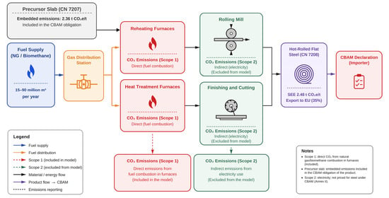
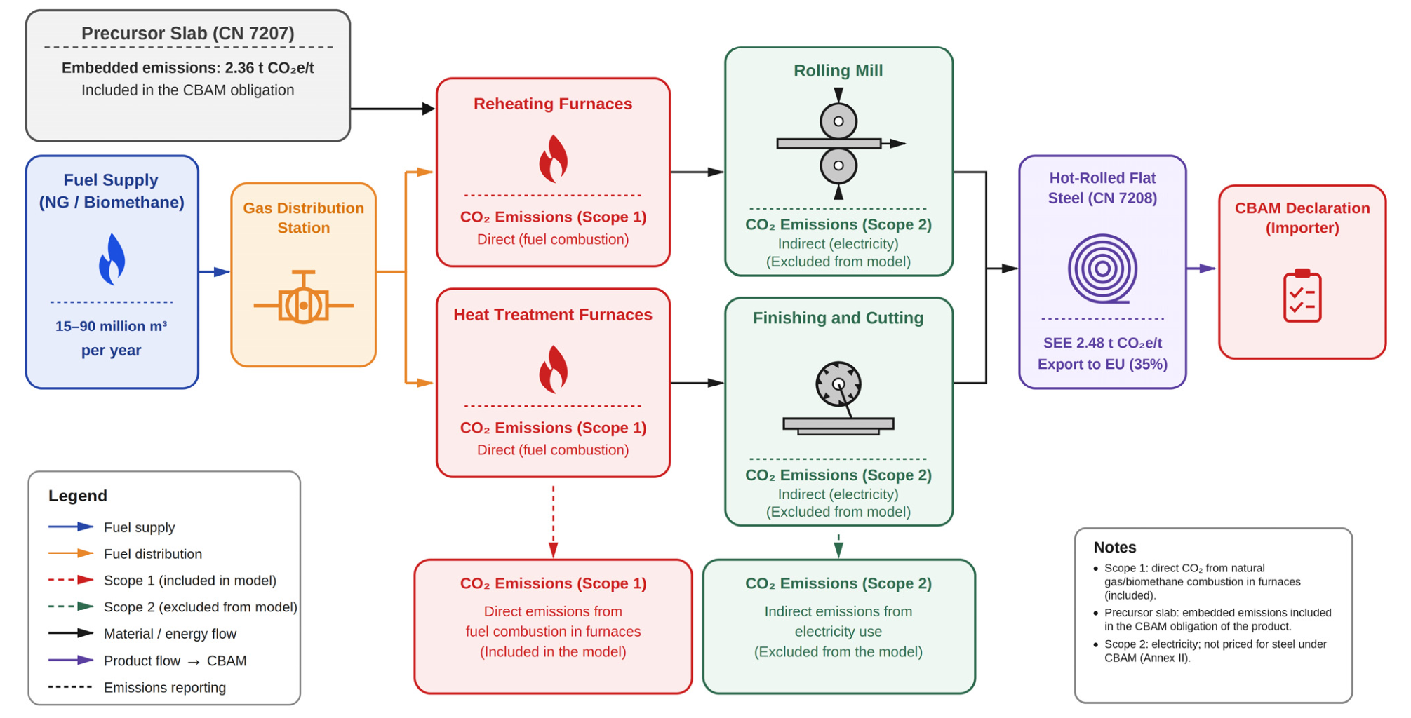
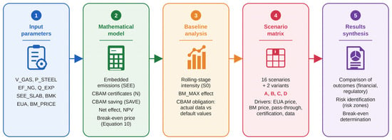
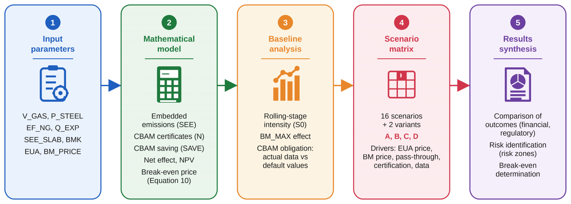
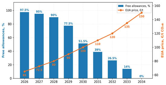
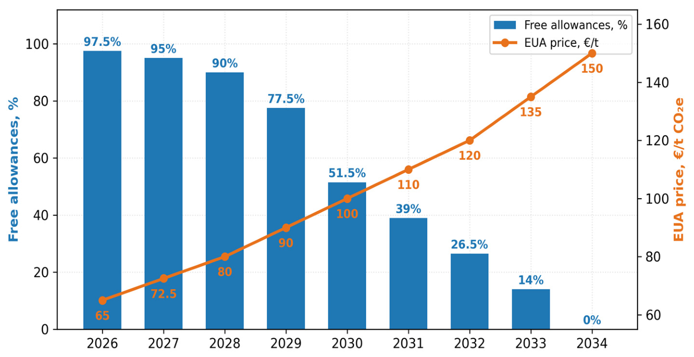
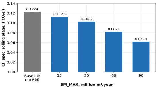
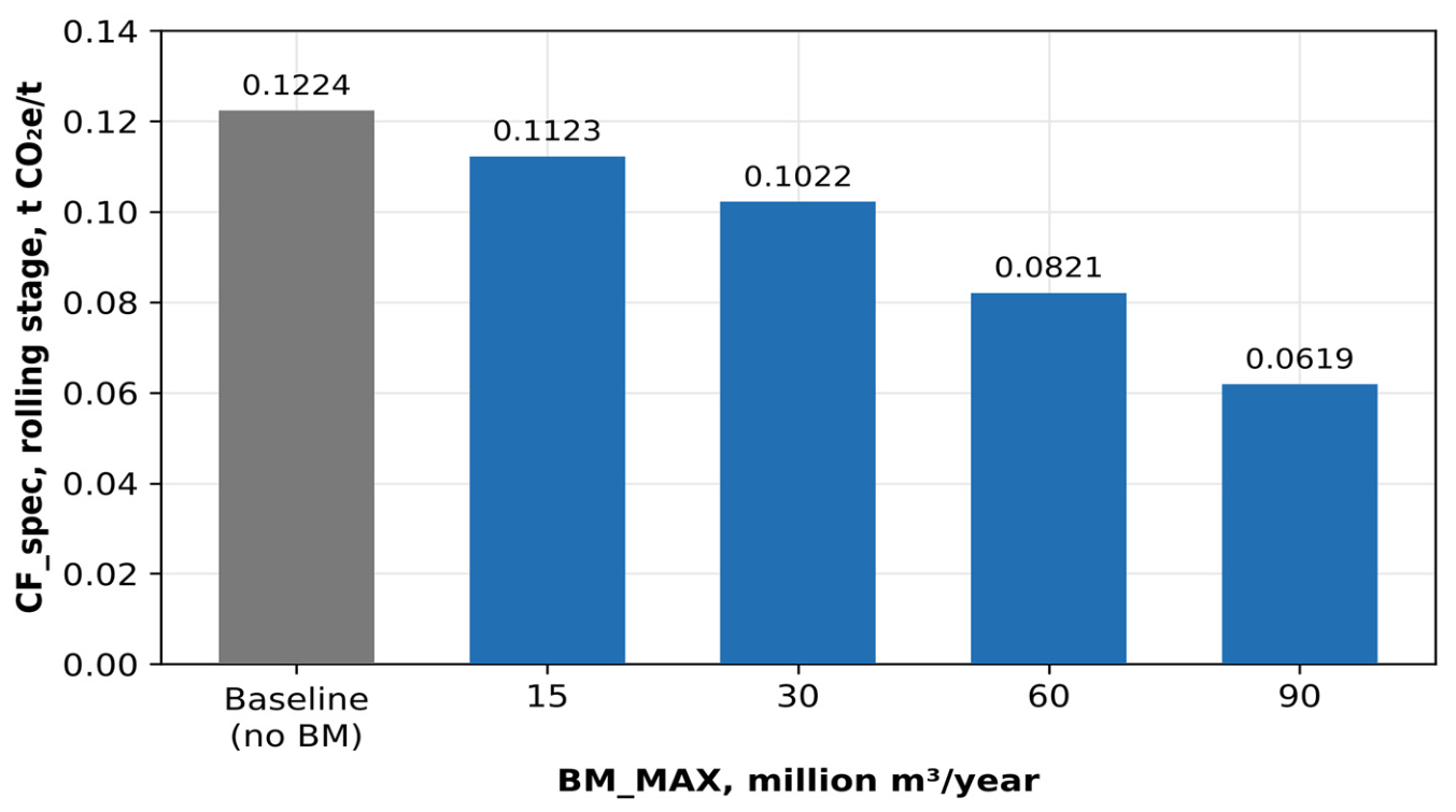
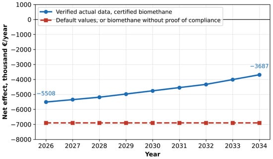
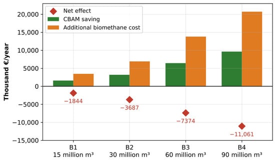
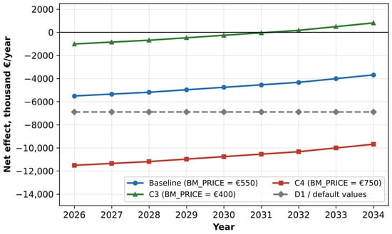
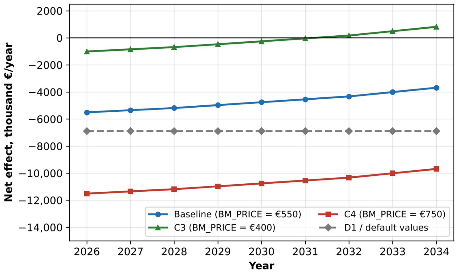
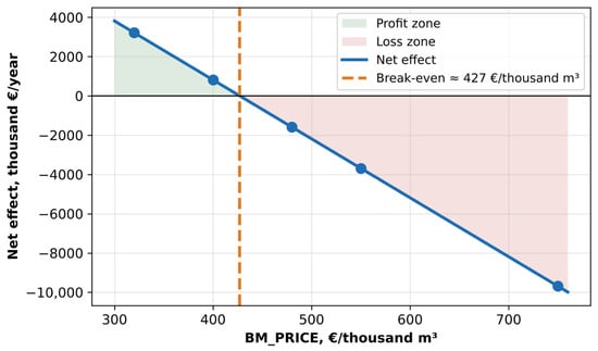
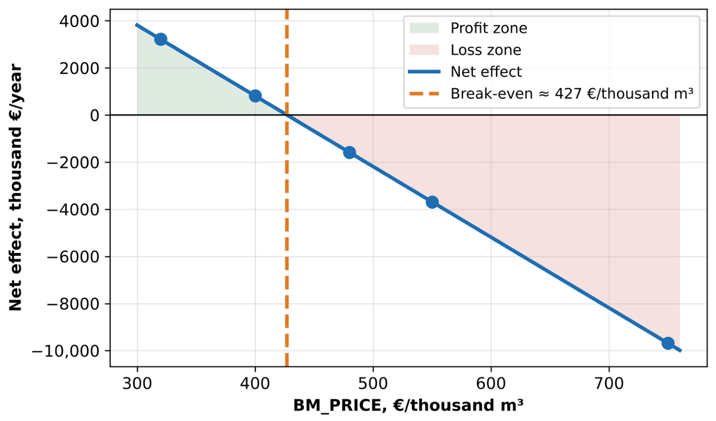
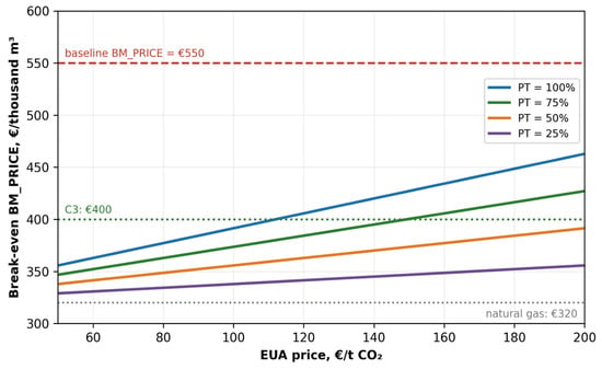
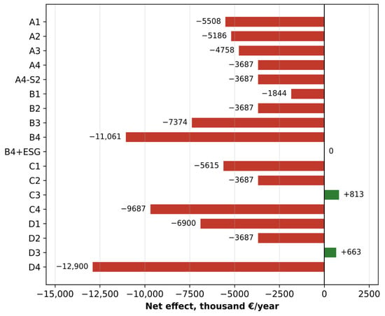
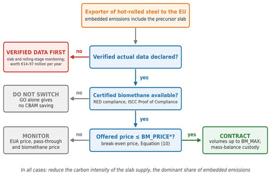

Disclaimer/Publisher’s Note: The statements, opinions and data contained in all publications are solely those of the individual author(s) and contributor(s) and not of MDPI and/or the editor(s). MDPI and/or the editor(s) disclaim responsibility for any injury to people or property resulting from any ideas, methods, instructions or products referred to in the content. |
© 2026 by the authors. Licensee MDPI, Basel, Switzerland. This article is an open access article distributed under the terms and conditions of the Creative Commons Attribution (CC BY) license.