Optimization Study on Integrated Energy Mutual Aid–Response Considering Multi-Energy Flow Carbon Responsibility Allocation

Abstract

Improving the sustainability of regional integrated energy systems requires carbon signals that reflect the coupled use of electricity, cooling, and heating. In this paper, we propose a multi-energy flow responsibility factor construction method that accounts for carbon responsibility allocation on both the source and demand sides, and employ it as a low-carbon signal within a multi-regional collaborative optimization framework for mutual aid and response. First, a dynamic weighting mechanism based on real-time electricity–heat (cooling) supply–demand matching is established to enable fine-grained allocation of carbon responsibility among the three energy flows. Subsequently, a joint capacity configuration and operational optimization model is developed by integrating low-carbon demand response (LCDR) with carbon trading. The proposed approach is then validated using measured data from the Higashida area of Kitakyushu, Japan, to investigate the low-carbon response benefits under two operating scenarios: independent operation and mutual aid operation across multiple systems. The results demonstrate that the proposed method effectively shifts loads toward low-carbon periods and enhances local photovoltaic utilization. Specifically, compared with interconnected operation without LCDR (Case 1), the proposed LCDR method reduces carbon emissions by 1.4%. Furthermore, compared with independent operation with LCDR (Case 3), the proposed multi-regional interconnection strategy reduces external power purchases by 18.2% and lowers total operational costs by 4.1%. Although this interconnected strategy leads to a moderate 5.5% increase in local carbon emissions due to higher local natural gas consumption, it represents a rational trade-off that significantly enhances system economic viability and energy autonomy, achieving the greatest overall benefit.

1. Introduction

The global transition toward clean energy and deep decarbonization has become a pressing challenge in mitigating climate change [1,2]. Against this backdrop, integrated energy systems (IESs), which eliminate the boundaries between individual energy subsystems and enable coordinated planning and operation of multiple energy carriers such as electricity, heat, cooling, and gas, are widely recognized as a key approach for enhancing overall energy efficiency and facilitating large-scale renewable energy integration [3,4]. IESs can be classified into different levels according to geographical scope [5], and this study focuses on regional integrated energy systems (RIESs). RIESs achieve cascade utilization and multi-energy complementarity near the load side and have become an important form of energy system innovation at the urban and community levels [6,7]. For RIES planning, sustainability therefore involves coordinating renewable energy use and energy conversion efficiency with the economic feasibility of meeting local demand.

The core of RIESs lies in multi-energy flow coupling and collaborative optimization. Researchers worldwide have conducted extensive research on this. Early studies mainly focused on system architecture design and basic modeling [8]. With the deepening of research, optimization objectives have expanded from a single economic dimension to multiple dimensions, including reliability and environmental protection [9]. In terms of modeling methods, mixed-integer linear programming has become an effective tool for solving IES configuration and operational problems [10]. Yang et al. [11] linked hourly multi-energy load forecasting with station siting, network routing, and capacity optimization, accounting for the complementary characteristics of electricity, heating, and cooling demands. Existing studies have shown that the interconnection structure of multiple RIESs can effectively alleviate the problem of redundant equipment capacity caused by mismatched peak and valley loads in a single region [12,13] and improve system economics and operational resilience through cross-regional reconstruction of energy flows [14], which is particularly significant given the increasing penetration of renewable energy. However, the aforementioned studies mainly optimize the supply-side system, treating loads as rigid parameters and ignoring the enormous potential of demand-side resources [15], especially demand response (DR) based on prices [16,17,18] or carbon signals [19,20,21], in improving system flexibility, economics, and low-carbon performance.

Price-based DR has been proven effective in peak-valley regulation, but its main goal is economic optimization [22]. Low-carbon demand response (LCDR) uses carbon signals to guide load adjustment [23]. Ma et al. [24] combined dynamic carbon factors obtained by carbon flow tracking with time-of-use tariffs in a bi-level model of regional power grid operators and load aggregators, improving economic and emission-reduction performance through source-load coordination. Their case study illustrated the benefits of using both signals. Zhang et al. [25] constructed a full-process carbon emission flow model, introduced an LCDR mechanism, took node carbon intensity as an incentive signal, and proposed a low-carbon economic dispatch model for IESs that balances economics and emission reduction effects. The results showed that LCDR can significantly reduce system carbon emissions and operational costs while ensuring energy supply stability. Huang et al. [26] established a low-carbon economic dispatch framework for distributed energy systems based on carbon emission flow and Shapley value allocation. By clearly assigning node carbon responsibilities to the load side and combining demand response with a carbon trading mechanism, they effectively reduced system carbon emissions and total costs, verifying the feasibility and coordination of user-side participation in low-carbon regulation. Su et al. [27] further established a time-varying carbon flow model and a model of users’ willingness to participate in low-carbon demand response in the regional integrated energy service system. Using a multi-factor incentive signal composed of dynamic electricity prices, carbon emission factors, and renewable energy absorption levels, they guided users to actively adjust loads during low-carbon periods, realizing “source-load” collaborative low-carbon optimization and significantly improving renewable energy utilization efficiency. Most of the above studies are based on the “carbon emission flow” theory [28,29], linking dynamic carbon signals with real-time power flow, which addresses the lack of temporal variability in traditional static carbon emission factors. However, these methods struggle to reflect the real-time supply and demand status of the system and have high computational complexity. To address these limitations, Jiang et al. [30] introduced the concept of a dynamic carbon emission responsibility factor (DCERF), which allocates carbon responsibility based on real-time generator output and grid conditions. This method distinguishes between “must-run” thermal generation during low-load periods and peak-load regulation behavior, enabling dynamic transfer of carbon responsibility between producers and consumers. The DCERF satisfies balance, consistency, and sustainability principles while offering a highly responsive low-carbon signal for end users.

Although substantial progress has been made, existing studies still have limitations. Carbon emission flow theories [28,29] and Shapley value allocation methods [26] provide solid foundations for tracing carbon responsibilities; however, they either require complex network calculations that struggle to capture real-time multi-energy dynamics, or, in game-theoretic methods, encounter increased computational challenges as the scale of the system expands. Furthermore, the existing DCERF [30], while effective for pure power grids, fails to account for the strong electricity–heat coupling inherent in RIESs, particularly when CHP units are involved. Additionally, most current LCDR mechanisms are guided by electricity-only carbon signals and do not comprehensively reflect multi-energy flow interactions.

To address these gaps and support regional energy sustainability, this paper develops a dynamic carbon emission responsibility factor tailored for RIESs and employs it as a low-carbon signal for LCDR. The main innovative contributions are explicitly summarized as follows:

(1) A multi-energy flow carbon responsibility allocation method based on source–demand dynamic carbon responsibility factors is proposed, extending beyond traditional DCERF and Shapley value methods. Unlike pure network flow tracking or game theory, this method enables the decoupling of electricity and heat outputs of CHP units using a dynamic weighting factor based on real-time heat supply–demand matching. It reasonably attributes heterogeneous energy flow responsibilities and guides the spatiotemporal shifting of electrical loads to achieve improved multi-energy matching.

(2) A joint capacity–operation optimization model coordinating multi-regional interconnection and carbon trading is constructed. By integrating the proposed multi-energy flow LCDR signal (Cs)—which considers external electricity, CHP coupling, and inter-system exchanges—this model reveals the synergistic influence mechanism of mutual aid and response on system economic performance and carbon emission reduction, significantly advancing traditional LCDR frameworks.

2. Regional Integrated Energy System

2.1. System Architecture

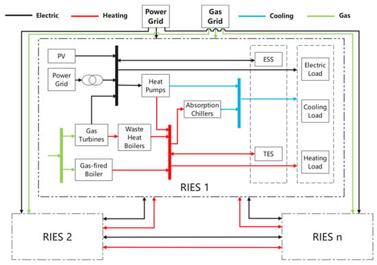
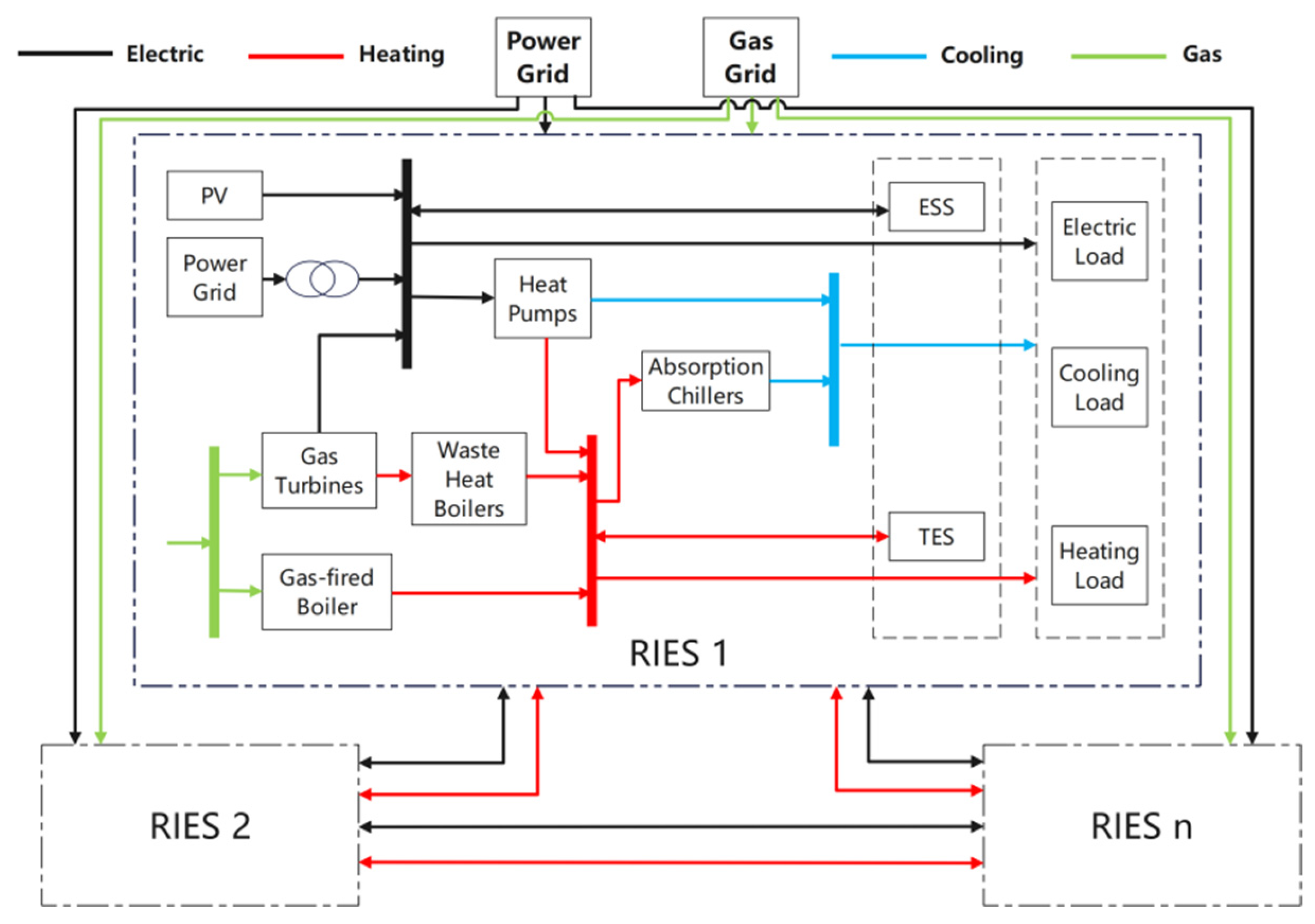
The basic structural topology of the regional integrated energy system (RIES) investigated in this study is illustrated in Figure 1. On the demand side, the system mainly comprises electricity, heating, and cooling loads. Energy supply in the RIES is primarily provided by the external power grid, the natural gas network, and photovoltaic (PV) generation. The main energy conversion devices include combined cooling, heating, and power (CCHP) units and gas boilers, while the energy storage facilities consist of electrical energy storage and thermal energy storage systems. Electrical loads are supplied by gas turbines and PV generation, with any deficit supplemented by the power grid. Heating demands are met by waste heat boilers, gas boilers, and heat pumps, whereas cooling demands are satisfied by absorption chillers and heat pumps. In addition, different RIESs can exchange electricity and thermal energy through interconnection pipelines, enabling mutual energy support and complementary operation.

Figure 1. Internal topology of the regional integrated energy system.

2.2. System Model Formulation

2.2.1. Equipment Models

The following models describe the input–output relations and energy-state equations for the energy equipment [31,32]. The time index is $t$, and the time-step duration is $1 \mathrm{h}$. Power variables are expressed in kW, stored energy and storage capacities are expressed in kWh, and efficiencies, coefficients of performance (COPs), and heat-to-power ratios are dimensionless. Regional indices are omitted for clarity; the relations apply to each RIES separately. Natural gas inputs are expressed as fuel-energy input powers rather than volumetric flow rates.

• Combined heat and power unit

The CHP unit converts natural gas input into electrical power and recoverable thermal power:

$$P_{chp}(t)={\eta }_{chp}^e{P}_{chp}^{gas}(t)$$

(1)

$$H_{\mathrm{c}\mathrm{h}\mathrm{p}}(t)=r_{\mathrm{c}\mathrm{h}\mathrm{p}}^{h/e}{P}_{\mathrm{c}\mathrm{h}\mathrm{p}}(t)$$

(2)

Here, $P_{chp}(t)$ and $H_{chp}(t)$ are the electrical and thermal outputs, respectively; $P_{chp}^{gas}(t)$ is the natural gas input power; ${\eta }_{chp}^e$ is the electrical efficiency; and ${\mathrm{r}}_{\mathrm{c}\mathrm{h}\mathrm{p}}^{\mathrm{h}/\mathrm{e}}$ is the heat-to-power ratio. If a separate thermal efficiency ${\eta }_{\mathrm{c}\mathrm{h}\mathrm{p}}^h$ is used, the definitions satisfy $r_{\mathrm{c}\mathrm{h}\mathrm{p}}^{h/e}={\eta }_{\mathrm{c}\mathrm{h}\mathrm{p}}^h/{\eta }_{\mathrm{c}\mathrm{h}\mathrm{p}}^e$. The heat-to-power ratio describes physical energy conversion and is distinct from the carbon-responsibility allocation coefficient.

• Absorption chiller

The absorption chiller uses thermal energy to produce cooling:

$$C_{ac}(t)={\eta }_{ac}{H}_{ac}(t)$$

(3)

Here, $C_{ac}(t)$ is the cooling output, and $H_{ac}(t)$ is the thermal input. The coefficient ${\eta }_{ac}$ is the ratio of cooling output to thermal input.

• Gas boiler

The gas boiler supplies heat according to the following:

$$H_{gb}(t)={\eta }_{gb}^h{P}_{gb}^{gas}(t)$$

(4)

Here, $H_{gb}(t)$ is the thermal output, $P_{gb}^{gas}(t)$ is the natural gas input power, and ${\eta }_{gb}^h$ is the thermal efficiency.

• Heat pump

The heating and cooling outputs of the heat pump are represented separately:

$$H_{hp}(t)={\eta }_{hp,h}{P}_{hp,h}(t)$$

(5)

$$C_{hp}(t)={\eta }_{hp,c}{P}_{hp,c}(t)$$

(6)

Here, $P_{hp,h}(t)$ and $P_{hp,c}(t)$ are the electrical inputs for heating and cooling, respectively; $H_{hp}(t)$ and $C_{hp}(t)$ are the corresponding outputs; and ${\eta }_{hp,h}$ and ${\eta }_{hp,c}$ are the heating and cooling ${\mathrm{C}\mathrm{O}\mathrm{P}}_s$. When both input components are represented in the model, the total heat pump electrical consumption in the electricity balance is defined as follows:

$$P_{\mathrm{h}\mathrm{p}}(t)=P_{\mathrm{h}\mathrm{p},h}(t)+P_{\mathrm{h}\mathrm{p},c}(t)$$

(7)

Equation (7) defines the total electrical consumption; it does not itself impose restrictions on simultaneous heating and cooling.

• Photovoltaic generation

The photovoltaic (PV) formulation below separates the preprocessing of a unit capacity generation profile from the installed capacity decision. The cell temperature is estimated from the ambient temperature and plane-of-array irradiance:

$$T_{cell}(t)=T_{air}(t)+{\displaystyle \frac{G_{surf}(t)}{800}}\times (NOCT-20)$$

(8)

The reference module direct current output is expressed as follows:

$$P_{dc}(t)=P_{dc,0}\times {\displaystyle \frac{G_{surf}(t)}{G_{ref}}}\times \left[1+{\gamma }_{pdc}\times (T_{cell}(t)-T_{ref})\right]$$

(9)

The alternating-current output before other system losses is expressed as follows:

$$P_{ac,raw}(t)=P_{dc}(t)\times {\eta }_{inv}$$

(10)

The normalized output profile and the installed system output are expressed as follows:

$$p_{\mathrm{p}\mathrm{v},unit}(t)={\displaystyle \frac{P_{\mathrm{a}\mathrm{c},raw}(t)(1-\mathrm{c})}{P_{\mathrm{d}\mathrm{c},0}}}$$

(11)

$$P_{\mathrm{p}\mathrm{v}}(t)={Cap}_{\mathrm{p}\mathrm{v}}{p}_{\mathrm{p}\mathrm{v},unit}(t)$$

(12)

Here, $T_{air}(t)$ and $T_{cell}(t)$ are the ambient and cell temperatures in degrees Celsius; $G_{surf}(t)$ is the plane-of-array irradiance, and $G_{\mathrm{r}\mathrm{e}\mathrm{f}}$ is the reference irradiance, both in $\mathrm{W}\hspace{0.17em}{\mathrm{m}}^{-2}$; NOCT is the nominal operating cell temperature, and $T_{\mathrm{N}\mathrm{O}\mathrm{C}\mathrm{T},ref}$ is its reference ambient temperature of 20 °C; $P_{dc,0}$ is the reference module rated direct current power in kW; ${\gamma }_{pdc}$ is the power temperature coefficient in ${\mathrm{K}}^{-1}$; $T_{ref}$ is the reference cell temperature; ${\eta }_{inv}$ is the inverter conversion efficiency; and $c$ is the fractional system loss. The normalized profile $p_{\mathrm{p}\mathrm{v},unit}(t)$ has units of kW/kW, and ${Cap}_{\mathrm{p}\mathrm{v}}$ is the installed PV capacity in kW. The time-dependent profile is computed before optimization, so Equation (12) is linear in the installed capacity.

• Electrical energy storage

$$E_{t+1}=(1-{\theta }^e)E_t+({\eta }_c^e{P}_{c,t}-P_{disc,t}/{\eta }_{disc}^e)∆t$$

(13)

The state of charge is defined as follows:

$${SOC}_t={\displaystyle \frac{E_t}{E_{cap}}}$$

(14)

Here, $E_t$ is stored electrical energy in kWh; $E_{cap}$ is the installed electrical storage capacity in kWh; $P_{c,t}$ and $P_{disc,t}$ are the charging and discharging powers in kW, respectively; ${\eta }_c^e$ and ${\eta }_{disc}^e$ are the corresponding efficiencies; and ${\theta }^e$ is the fractional standing loss per time step. The SOC definition applies when $E_{\mathrm{c}\mathrm{a}\mathrm{p}}> 0$; it can be expressed through equivalent energy bounds in a capacity-planning model to avoid division by a decision variable. The charging/discharging power limits, mutual-exclusion constraints, and $SOC$ bounds are presented in Section 4.2.2.

• Thermal energy storage

The stored thermal energy evolves according to the following:

$$H_{t+1}=(1-{\theta }^h)H_t+({\eta }_c^h{H}_{c,t}-H_{disc,t}/{\eta }_{disc}^h)∆t$$

(15)

Here, $H_t$ is stored thermal energy in kWh; $H_{c,t}$ and $H_{disc,t}$ are the charging and discharging thermal powers in kW, respectively; ${\eta }_c^h$ and ${\eta }_{disc}^h$ are the corresponding efficiencies; and ${\theta }^h$ is the fractional standing loss per time step. The stored energy variable $H_t$ is distinct from thermal power variables such as $H_{\mathrm{c}\mathrm{h}\mathrm{p}}(t)$.

• Efficiency assumptions

In Equations (1)–(7), the conversion efficiencies, heat-to-power ratio, and ${\mathrm{C}\mathrm{O}\mathrm{P}}_s$ are fixed coefficients. These equations do not explicitly represent part-load efficiency curves or temperature-dependent heat pump ${\mathrm{C}\mathrm{O}\mathrm{P}}_s$. This approximation preserves linear input–output relations but does not capture equipment performance changes under off-design conditions. In contrast, the PV preprocessing in Equations (8)–(11) accounts for irradiance and cell-temperature variations. The storage equations represent energy inventory, standing losses, and conversion losses; they do not themselves describe aging-related capacity fade or equipment replacement. The gas boiler thermal efficiency is 0.9, the absorption chiller $\mathrm{C}\mathrm{O}\mathrm{P}$ is 1.2, and the heat pump heating and cooling ${\mathrm{C}\mathrm{O}\mathrm{P}}_s$ are 3.0 and 2.8, respectively.

2.2.2. Interconnection Pipeline Model

To account for transmission losses during energy exchange between RIESs, models for electricity and thermal interconnection lines are established. The energy loss functions characterize the transmission states between energy station i and energy station j, expressed as follows:

$${\mathrm{P}}_{\mathrm{i}-\mathrm{j},t}=(1-{\mathrm{f}}_{\mathrm{i}-\mathrm{j}}^{\mathrm{e}}){\mathrm{P}}_{\mathrm{i}-\mathrm{j},t}^{\ast }$$

(16)

$${\mathrm{H}}_{\mathrm{i}-\mathrm{j},t}=(1-{\mathrm{f}}_{\mathrm{i}-\mathrm{j}}^{\mathrm{h}}){\mathrm{H}}_{\mathrm{i}-\mathrm{j},t}^{\ast }$$

(17)

$${\mathrm{f}}_{\mathrm{i}-\mathrm{j}}^{\mathrm{e}/\mathrm{h}}={\mathrm{L}}_{\mathrm{i}-\mathrm{j}}^{\mathrm{e}/\mathrm{h}}{\phi }_{\mathrm{e}/\mathrm{h}}$$

(18)

Here, ${\mathrm{P}}_{\mathrm{i}-\mathrm{j},t}$ and ${\mathrm{H}}_{\mathrm{i}-\mathrm{j},t}$ denote the actual electrical and thermal power received by RIES j from RIES i at time t after accounting for transmission losses (kW), respectively; ${\mathrm{P}}_{\mathrm{i}-\mathrm{j},t}^{\ast }$ and ${\mathrm{H}}_{\mathrm{i}-\mathrm{j},t}^{*}$ denote the electrical and thermal power transmitted from RIES I to RIES j (kW), respectively; ${\mathrm{f}}_{\mathrm{i}-\mathrm{j}}^{\mathrm{e}}$ and ${\mathrm{f}}_{\mathrm{i}-\mathrm{j}}^{\mathrm{h}}$ are the loss rates for electrical and thermal power transmission, respectively; ${\mathrm{L}}_{\mathrm{i}-\mathrm{j}}^{\mathrm{e}}$ and ${\mathrm{L}}_{\mathrm{i}-\mathrm{j}}^{\mathrm{h}}$ represent the lengths of electrical and thermal transmission lines between the two RIESs (km), respectively; and ${\phi }_{\mathrm{e}}$ and ${\phi }_{\mathrm{h}}$ are the loss coefficients per unit distance.

It should be noted that Equation (18) applies a steady-state linear approximation for transmission losses, whereas actual heat dissipation is dynamic and influenced by operating temperatures and flow rates. This simplification is adopted as a practical approach for macroscopic system-level planning, considering the relatively short interconnection distance in this case study.

In the simulations, the line length is set as ${\mathrm{L}}_{\mathrm{i}-\mathrm{j}}=1.25$ km. The unit distance loss coefficient for electrical transmission is $\phi =0.03\%$/km and that for thermal transmission is $\phi =0.05\%$/km [33] based on the existing engineering literature.

3. Dynamic Carbon Emission Responsibility Factors and LCDR Modeling

The regional integrated energy system (RIES) involves the coordinated supply of multiple energy carriers, including electricity, heat, and cooling. Owing to thermal inertia and other operational constraints of thermal systems, heating loads typically do not participate in demand response (DR). Cooling loads, however, are supplied through electricity-driven devices (heat pumps) and heat-driven devices (absorption chillers). As a result, the system can be equivalently modeled as comprising electricity and heat loads only. Accordingly, unless otherwise specified, the low-carbon demand response (LCDR) loads considered in this study refer exclusively to electrical loads.

The key to enabling demand-side participation in low-carbon operation lies in constructing a dynamic carbon signal that accurately reflects the real-time operating state of the system. To this end, this study first develops carbon emission responsibility factor models for electricity purchased from the external power grid and for combined heat and power (CHP) units. Subsequently, by jointly considering photovoltaic (PV) generation and inter-system energy exchanges, a dynamic electricity supply carbon emission responsibility factor for regional integrated energy systems is established, providing a foundation for the implementation of low-carbon demand response.

3.1. Dynamic Carbon Emission Responsibility Factor for Purchased Electricity

This study introduces the DCERF $C_r$ as a guiding signal for LCDR when the system purchases electricity from the external power grid. Its core idea is to convert the real-time supply–demand relationship of the power system into a carbon cost signal on the user side through dynamic allocation of carbon emission responsibilities; $C_r$ is calculated in real time based on the operating status of each power source, reflecting the real-time carbon responsibility per unit of electricity consumption, in kg CO₂/kWh.

During the operation of the power system, peak-shaving thermal power units during valley periods usually cannot be shut down and can only operate at the minimum load to ensure rapid response when the load recovers. At this time, even if wind and solar power generation is sufficient, some new energy power often needs to be curtailed to maintain the minimum power of thermal power units. This minimum operating power is not intended to meet current electricity demand but to provide the spinning reserve required for power grid regulation. Therefore, the carbon emissions generated by thermal power units during spinning reserve operation should not be borne by current valley users but should be included in the emission responsibility of users during future peak load periods. This means that during peak periods, electricity consumers not only bear the direct carbon emissions of the power sources at that time but also need to share the corresponding carbon emissions from the low-load operation of power sources during valley periods.

$C_r$ is embedded in the RIES optimization model as part of the low-carbon load response signal, which is expressed as follows:

$$C_r(t)={\displaystyle \frac{\sum P_k(t)C_{r,k}(t)}{\sum P_k(t)}}$$

(19)

where t is any time; ${\mathrm{P}}_{\mathrm{k}}(\mathrm{t})$ is the power generation of power source k, in kW; and $C_{r,k}$ is the carbon emission responsibility per unit of electricity transferred from power source k to the user side, in kgCO₂/kWh.

The method for calculating the carbon emission responsibility per unit of electricity transferred from each power source to the user side is as follows: since clean energy power sources such as wind power, photovoltaic power, and hydropower do not produce carbon emissions, their carbon emission responsibility factor per unit of electricity is the carbon emission responsibility factor $C_r$ of the power supply area where they are located at that time. The methods for calculating the carbon emission responsibility per unit of electricity for other power sources involved in this paper are as follows:

Coal-fired units:

$$C_{r,c}(t)={\epsilon }_c(t)C_{o,c}$$

(20)

CCGT units:

$$C_{r,g}(t)={\epsilon }_g(t)C_{o,g}$$

(21)

Inter-provincial tie lines:

$$C_{r,l}(t)=\{\begin{array}{c}{C}_r(t),P_l(t)>0\\ C_l(t),P_l(t)<0\end{array}$$

(22)

Here, t is any time; $C_{o,c}$ and $C_{o,g}$ are the average carbon emission factors of coal-fired thermal power units and CCGT thermal power units, respectively, in kg CO₂/kWh; ${\epsilon }_c$ and ${\epsilon }_g$ are the responsibility coefficients of coal-fired thermal power units and CCGT thermal power units, respectively; $P_l(t)>0$ indicates that the inter-provincial tie line sends out power; $P_l(t)<0$ indicates that the inter-provincial tie line receives power; and ${\mathrm{C}}_{\mathrm{l}}(\mathrm{t})$ is the carbon emission responsibility factor of the incoming power.

The responsibility coefficient of thermal power units is affected by the respective operating characteristics of different units. The output of thermal power units can indirectly reflect the supply–demand relationship of the power grid. To meet the sensitivity principle and enable $C_r$ to effectively stimulate the self-regulating behavior of electricity end users, it can be expressed by a logistic function relationship. Specifically, it grows exponentially in the initial stage of low load rate and reaches the peak growth rate at the average load rate of stable operation. Then, the growth rate gradually slows down until the maximum operating load rate. Its basic expression is noted as follows:

Coal-fired units:

$${\epsilon }_c(t)={\displaystyle \frac{L}{1+exp\{-K_c\cdot \left[P_c(t)/P_c^{max}-B_c\right]\}}}$$

(23)

CCGT units:

$${\epsilon }_g(t)={\displaystyle \frac{L}{1+exp\{-K_g\cdot \left[P_g(t)/P_g^{max}-B_g\right]\}}}$$

(24)

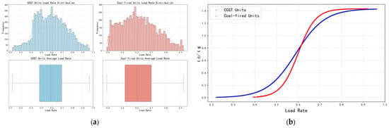
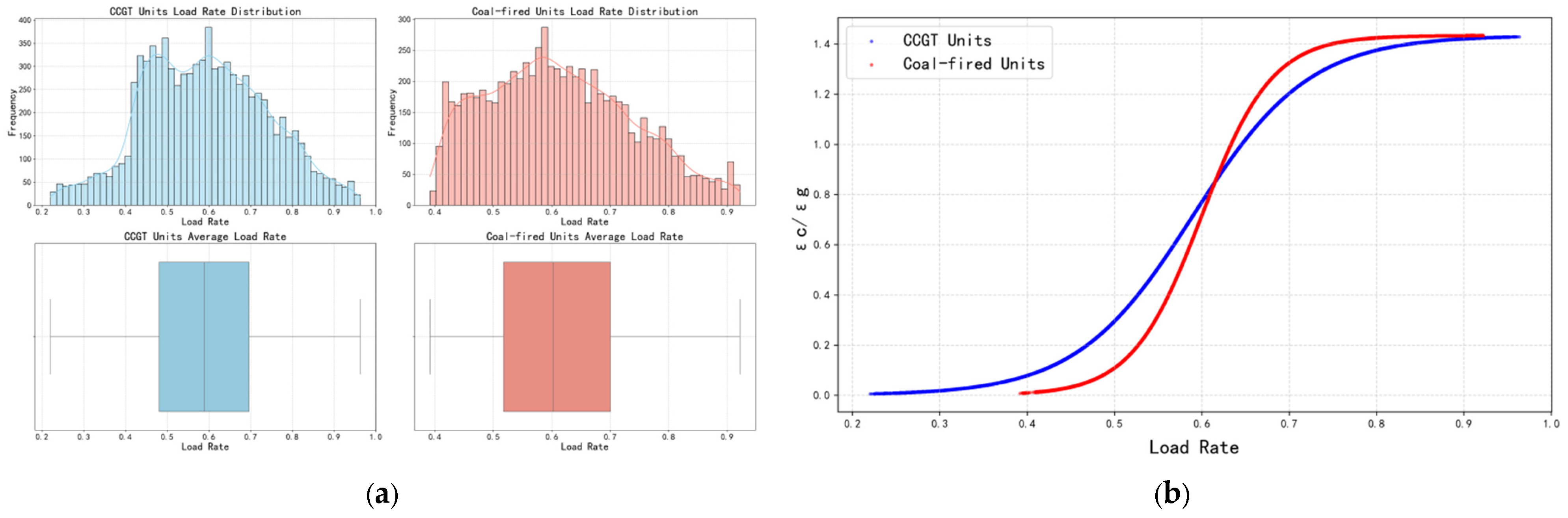
Here, t is any time; ${\mathsf{\epsilon }}_{\mathrm{c}}$ and ${\mathsf{\epsilon }}_{\mathrm{g}}$ are the responsibility coefficients of coal-fired and CCGT units, respectively, dimensionless; ${\mathrm{P}}_{\mathrm{c}}$ and ${\mathrm{P}}_{\mathrm{g}}$ are the power generation of coal-fired and CCGT units, respectively, in kW; ${\mathrm{P}}_{\mathrm{c}}^{\mathrm{m}\mathrm{a}\mathrm{x}}$ and ${\mathrm{P}}_{\mathrm{g}}^{\mathrm{m}\mathrm{a}\mathrm{x}}$ are the rated power of coal-fired and CCGT units, respectively, in kW; ${\mathrm{B}}_{\mathrm{c}}$ and ${\mathrm{B}}_{\mathrm{g}}$ are the annual average load rates of coal-fired units and CCGT units, respectively; and ${\mathrm{K}}_{\mathrm{c}}$ and ${\mathrm{K}}_{\mathrm{g}}$ are the function growth rates of the two units determined by the stable operating load rate range of the units. As illustrated in Figure 2a, the annual average load factor of the coal-fired units is approximately 60%, with a stable operating load range of 40–90%, whereas the CCGT units exhibit an annual average load factor of about 59% and a stable operating load range of 23–95%. Based on the known annual average load factors and stable operating ranges of the units, the parameters in Equations (23) and (24) are determined as ${\mathrm{B}}_{\mathrm{c}}$ = 0.60, ${\mathrm{B}}_{\mathrm{g}}$ = 0.59, ${\mathrm{K}}_{\mathrm{c}}$ = 25, and ${\mathrm{K}}_{\mathrm{g}}$ = 15.

Figure 2. Calculation results of parameters related to thermal power units. (a) Annual average load rate of thermal power units. (b) Relationship between load rate and carbon emission responsibility coefficient.

The data used to calculate the thermal unit parameters in Figure 2 were obtained from publicly available data for the Kyushu region of Japan and local field measurements.

The parameter L is determined based on the balance principle, under which the sum of carbon emission responsibilities on the production side equals zero over the annual time horizon, and the total carbon emissions generated on the production side are equal to the total carbon emission responsibilities allocated to the consumption side. Accordingly, the value of L is calculated to be 1.434, and the corresponding calculation procedure is described as follows:

Total carbon emission responsibilities on the production side:

$$S_{c,k}=\int P_k(t)\cdot \left[C_{0,k}(t)-C_r(t)\right]dt$$

(25)

In Equation (25), t is measured in h; $S_{c,k}$ denotes the accumulated production-side carbon responsibility of source k, in kg CO₂; $C_{0,k}(t)$ and $C_r(t)$ are carbon emission factors, in kg CO₂/kWh; and $P_k(t)$ is the output power of source k, in kW. Integration over time gives the accumulated carbon responsibility in kg CO₂.

Total carbon emission responsibilities on the consumption side:

$$T_c=\int P_T(t)\cdot C_r(t)dt$$

(26)

In Equation (26), $T_c$ denotes the accumulated consumption-side carbon responsibility over the annual horizon, in kg CO₂; $P_T(t)$ is the electrical power supplied to consumers, in kW; $C_r(t)$ is the electricity carbon responsibility factor, in kg CO₂/kWh; and t is measured in h.

The calculated responsibility coefficients of thermal power units are illustrated in Figure 2b. The results are consistent with the preceding analysis. When the units operate at low load levels (i.e., under minimum load operation), carbon emission responsibility is not transferred to the user side. Within the stable operating load range, both ${\epsilon }_c$ and ${\epsilon }_g$ increase rapidly as the unit load level rises. When the units operate at their maximum load levels, the carbon emission responsibility transferred to the user side reaches its peak.

Based on the above-determined calculation methods of power carbon emission responsibilities transferred from various power sources to the consumption side, $C_r$ can be expressed as follows:

$$\begin{array}{c}{C}_r(t)=[\sum P_c(t)\cdot C_{r,c}(t)+\sum P_g(t)\cdot C_{r,g}(t)-\sum P_l(t)\cdot C_{r,l}(t)]/\\ \left[\sum P_c(t)+\sum P_g(t)-P_l(t)\right]\end{array}$$

(27)

Given that the power of the inter-provincial tie line $P_l$ in the region studied in this paper is always positive, i.e., power is transmitted outward, Equation (27) can be simplified according to Equation (22) as follows:

$$\begin{array}{c}{C}_r(t)=[\sum P_c(t)\cdot C_{r,c}(t)+\sum P_g(t)\cdot C_{r,g}(t)]/\\ \left[\sum P_c(t)+\sum P_g(t)\right]\end{array}$$

(28)

Based on the above analysis, the calculated ${\mathrm{C}}_{\mathrm{r}}$ varies dynamically with time and the overall supply–demand conditions of the power system, thereby reflecting the carbon emission responsibility associated with each unit of electricity purchased by RIESs.

3.2. Dynamic Carbon Emission Responsibility Factor of CHP Electricity Supply

CHP units simultaneously produce electricity and heat from a common fuel input, requiring an allocation rule to assign the resulting carbon emissions to the two outputs. This study adopts energy-based allocation as the baseline for the subsequent heat-matching adjustment. The baseline assigns emissions in proportion to electrical and thermal output expressed on a consistent energy basis; it does not imply that electricity and heat have equivalent thermodynamic quality. The baseline allocation is expressed as follows:

$$C_{cchp,t}^{total}=C_{gas}{P}_{cchp,t}^{gas}$$

(29)

$${\alpha }_{e,t}^0={\displaystyle \frac{P_{chp,t}}{P_{chp,t}+H_{chp,t}}}, {\alpha }_{h,t}^0={\displaystyle \frac{H_{chp,t}}{P_{chp,t}+H_{chp,t}}}$$

(30)

$$C_{e,t}^0={\alpha }_{e,t}^0{C}_{cchp,t}^{total}, C_{h,t}^0={\alpha }_{h,t}^0{C}_{cchp,t}^{total}$$

(31)

In Equations (29)–(31), $P_{cchp,t}^{gas}$ is the natural gas energy input power, and $P_{chp,t}$ and $H_{chp,t}$ are the electrical and thermal output powers, respectively, all in kW. $C_{gas}$ is the natural gas emission factor, in kg CO₂/kWh. Consequently, $C_{cchp,t}^{total}$, $C_{e,t}^0$, and $C_{h,t}^0$ represent the total and allocated carbon emission rates, in kg CO₂/h. The allocation coefficients ${\alpha }_{e,t}^0$ and ${\alpha }_{h,t}^0$ are dimensionless. Multiplication by the time-step duration of 1 h gives the corresponding emission quantities in kg CO₂.

It should be noted that from a strict thermodynamic perspective, electricity is high-grade energy (exergy), whereas heat is low-grade energy (enthalpy). The energy-based allocation method (Equations (29)–(31)) treats them equally by simply adding their energy outputs, which has inherent thermodynamic limitations.

Alternative allocation methods were not adopted for the following two main reasons:

(1) Model compatibility: Exergy-based allocation methods (e.g., the Carnot factor method) require detailed thermodynamic parameters, which are typically not modeled in macroscopic MILP optimization models. Avoided-emission methods (e.g., the Finnish method) rely on predefined reference efficiencies that are difficult to integrate endogenously into the optimization.

(2) Objectivity: Avoided-emission methods rely on a subjectively chosen reference baseline, which would introduce significant uncertainty and potentially distort the carbon responsibility evaluation.

Conversely, the energy-based method is transparent, data-efficient, and highly compatible with the system-level energy flow variables used in this study, making it the most practical approach for the proposed optimization framework.

However, in practical operation, mismatches between electricity and heat load profiles may lead to situations in which the heat produced by CHP units cannot be fully utilized, or, alternatively, heat supply becomes insufficient and must be supplemented by gas boilers. These conditions result in suboptimal system energy utilization efficiency. To address this issue, a dynamic carbon emission responsibility factor for CHP electricity supply is developed to encourage electrical loads to participate in low-carbon demand response (LCDR), thereby improving overall system energy efficiency.

Building on the conventional energy-based allocation method, a dynamic weighting factor based on the degree of heat supply–demand matching is introduced to adjust the allocation of carbon emission responsibility between the electricity and heat outputs of CHP units. Two typical operating conditions, namely, heat surplus and heat deficit, are explicitly characterized and mapped to adjustment coefficients for the electricity-side carbon emission responsibility. When heat surplus occurs, a larger portion of carbon emission responsibility is shifted to the electricity side, thereby discouraging electricity consumption and reducing CHP output to mitigate excess heat generation. Conversely, when heat supply is insufficient, the electricity-side carbon emission responsibility is appropriately reduced, making electricity appear more “low-carbon,” which incentivizes electricity consumption, increases CHP heat production, and reduces reliance on less efficient gas boilers. The detailed model formulation is described as follows.

The total heat demand $H_t^{dem}$, effective heat utilization of the CHP unit $H_t^{use}$, heat surplus $H_t^s$, and heat deficit $H_t^{def}$ are defined as follows:

$$H_t^{dem}=L_h^t+H_{ac}^t+H_{i-j}^t$$

(32)

$$H_t^{use}=\mathit{min}(H_{chp,t},H_t^{dem})$$

(33)

$$H_t^s=\mathit{max}(0,H_{chp,t}-H_t^{dem})$$

(34)

$$H_t^{def}=\mathit{max}(0,H_t^{dem}-H_{chp,t})$$

(35)

In Equations (32)–(35), $L_h^t$, $H_{ac}^t$, and $H_{i-j}^t$ denote the heating load, thermal input to the absorption chiller, and thermal power exported to the neighboring RIES, respectively. $H_{chp,t}$ is the CHP thermal output. The resulting total thermal demand, utilized thermal output, surplus, and deficit are also power quantities. All these variables are expressed in kW. $H_{chp,t}$ denotes the heat output of the CHP unit.

To characterize the level of heat utilization, the heat surplus ratio ${\gamma }_t^s$ is defined to quantify the proportion of heat produced by the CHP unit that is not utilized, whereas the heat deficit ratio ${\gamma }_t^{def}$ is introduced to measure the proportion of total heat demand that remains unmet. These ratios are defined as follows:

$${\gamma }_t^s={\displaystyle \frac{H_t^s}{H_{chp,t}}}, {\gamma }_t^{def}={\displaystyle \frac{H_t^{def}}{H_t^{dem}}}$$

(36)

To reflect the impact of thermal energy utilization conditions on the allocation of carbon emission responsibility, the electricity-side dynamic weighting factor ${\omega }_{e,t}$ is defined as follows:

$${\omega }_{e,t}=1+{\gamma }_t^s-{\gamma }_t^{def}$$

(37)

A larger value of ${\gamma }_{\mathrm{t}}^{\mathrm{s}}$ (approaching 1) indicates a larger heat surplus, in which case a greater share of carbon emission responsibility should be allocated to electricity supply; therefore, ${\gamma }_t^s$ is added positively to the weighting factor. Conversely, a larger value of ${\gamma }_{\mathrm{t}}^{\mathrm{d}\mathrm{e}\mathrm{f}}$ (approaching 1) implies a more severe heat deficit. To encourage electricity consumption and stimulate CHP heat production, the electricity-side carbon emission responsibility is reduced; thus, ${\gamma }_{\mathrm{t}}^{\mathrm{d}\mathrm{e}\mathrm{f}}$ is incorporated with a negative sign.

Under the effect of the dynamic weighting factor, the carbon emission allocation coefficients for electricity and heat produced by the CHP unit are redefined as follows:

$${\alpha }_{e,t}={\displaystyle \frac{{\omega }_{e,t}{P}_{chp,t}}{{\omega }_{e,t}{P}_{chp,t}+H_t^{use}}}, {\alpha }_{h,t}={\displaystyle \frac{H_t^{use}}{{\omega }_{e,t}{P}_{chp,t}+H_t^{use}}}$$

(38)

where the sum of ${\alpha }_{\mathrm{e},t}$ and ${\alpha }_{\mathrm{h},t}$ equals 1, ensuring that the allocation of carbon emission responsibility satisfies the principle of total carbon emission balance.

Accordingly, the carbon emission responsibility per unit of electricity generated by the CHP unit (i.e., carbon intensity) can be calculated as follows:

$$C_{e,t}^{cchp}={\displaystyle \frac{{\alpha }_{e,t}{C}_{cchp,t}^{total}}{P_{chp,t}}}$$

(39)

Based on the above modeling framework, the proposed dynamic carbon emission responsibility factor for CHP electricity supply, ${\mathrm{C}}_{\mathrm{e},t}^{\mathrm{c}\mathrm{c}\mathrm{h}\mathrm{p}}$, enables dynamic adjustment of carbon emission responsibility between electricity and heat outputs while preserving the conservation of total carbon emissions of the CHP unit.

3.3. Dynamic Carbon Emission Responsibility Factor for RIES Electricity Supply

Based on the models developed in Section 3.1 and Section 3.2, the dynamic carbon emission responsibility factor for electricity supply in RIES, denoted as $C_s$, is defined as follows:

$${\mathrm{C}}_{\mathrm{s}}(\mathrm{t})={\displaystyle \frac{{\mathrm{C}}_{\mathrm{r}}(\mathrm{t}){\mathrm{P}}_{\mathrm{g}\mathrm{r}\mathrm{i}\mathrm{d}}(\mathrm{t})+{\mathrm{P}}_{\mathrm{c}\mathrm{h}\mathrm{p}}(\mathrm{t}){\mathrm{C}}_{\mathrm{e},t}^{\mathrm{c}\mathrm{c}\mathrm{h}\mathrm{p}}+{\mathrm{P}}_{\mathrm{j}-\mathrm{i}}(\mathrm{t})\ast {\mathrm{C}}_{\mathrm{s}}^{\ast }(\mathrm{t})}{{\mathrm{P}}_{\mathrm{g}\mathrm{r}\mathrm{i}\mathrm{d}}(\mathrm{t})+{\mathrm{P}}_{\mathrm{c}\mathrm{h}\mathrm{p}}(\mathrm{t})+{\mathrm{P}}_{\mathrm{p}\mathrm{v}}(\mathrm{t})+{\mathrm{P}}_{\mathrm{j}-\mathrm{i}}(\mathrm{t})}}$$

(40)

where t is any time; ${\mathrm{P}}_{\mathrm{g}\mathrm{r}\mathrm{i}\mathrm{d}}$ is the external purchased power, in kW; ${\mathrm{P}}_{\mathrm{c}\mathrm{h}\mathrm{p}}$ is the output power of CHP units, in kW; ${\mathrm{P}}_{\mathrm{p}\mathrm{v}}$ is the output power of PV, in kW; ${\mathrm{P}}_{\mathrm{j}-\mathrm{i}}$ is the electrical power input from other systems, in kW; and ${\mathrm{C}}_{\mathrm{s}}^{\ast }$ denotes the dynamic carbon emission responsibility factor of electricity supply in other RIESs, in kg CO₂/kWh.

It should be noted that the battery discharge power (${\mathrm{P}}_{\mathrm{d}\mathrm{i}\mathrm{s}\mathrm{c}}^{\mathrm{t}}$) is not explicitly included in Equation (40). As a temporal energy buffer, the energy storage system does not generate primary energy or direct emissions [34]. The carbon responsibility of the stored electricity is entirely allocated during the charging phase (reflected in the historical Cs(t) values when the battery acts as a load). During discharge, the battery meets a portion of the electricity demand, thereby partially replacing the output from carbon-emitting sources (such as grid purchases, CHP, and tie line transfers). This partial displacement is implicitly reflected in the reduced power output of these sources within Equation (40), thereby accurately updating the real-time carbon intensity of the system.

In summary, the constructed ${\mathrm{C}}_{\mathrm{s}}$ reflects the overall carbon emission level of the system under different operating conditions.

3.4. Low-Carbon Demand Response Model

${\mathrm{C}}_{\mathrm{s}}$ is used as the dynamic carbon signal to guide low-carbon demand response in the RIES, and the electrical load after response is expressed as follows:

$$L_{e,t}^{af}=L_{e,t}^{be}+{\beta }^{in}{L}_{e,t}^{in}-{\beta }^{out}{L}_{e,t}^{out}$$

(41)

$${\displaystyle {\sum }_{t=1}^{N_t}}{L}_{e,t}^{in}={\displaystyle {\sum }_{t=1}^{N_t}}{L}_{e,t}^{out}$$

(42)

$${\beta }^{in}+{\beta }^{out}\le 1$$

(43)

$$L_{e,t}^{in}={\alpha }^{in}{L}_{e,t}^{be}$$

(44)

$$L_{e,t}^{out}={\alpha }^{out}{L}_{e,t}^{be}$$

(45)

$$L_{e,t}^{in}={\displaystyle {\sum }_{\tau =max(0,t-24)}^{min(8759,t+24)}}{L}_{e,\tau }^{out}$$

(46)

where t is any time; $L_{e,t}^{af}$ and $L_{e,t}^{be}$ are the electrical load after participating in LCDR and the original electrical load before LCDR, respectively, in kW; and $L_{e,t}^{in}$ and $L_{e,t}^{out}$ are the power of transferable load incoming and outgoing, respectively, in kW. Equation (43) stipulates that transferable load cannot be incoming and outgoing at the same time; ${\alpha }^{in}$ and ${\alpha }^{out}$ are the proportions of the maximum transferable load to the original load. Equation (46) stipulated that load transfer must be completed within the same day; $N_t$ is the number of hours in the cycle, set to 8760 h a year.

The internal equivalent carbon cost/benefit associated with LCDR is given as follows:

$$f_{idr,t}={\lambda }_{idr}(L_{e,t}^{af}-L_{e,t}^{be})C_s(t)$$

(47)

where ${\lambda }_{\mathrm{i}\mathrm{d}\mathrm{r}}$ denotes the internal settlement price for carbon emission variations (CNY/kg CO₂). The term $({\mathrm{L}}_{\mathrm{e},t}^{\mathrm{a}\mathrm{f}}-{\mathrm{L}}_{\mathrm{e},t}^{\mathrm{b}\mathrm{e}}){\mathrm{C}}_{\mathrm{s}}(\mathrm{t})$ represents the change in carbon emissions before and after participating in LCDR.

When the load is shifted into period t, carbon emissions increase, and ${\mathrm{f}}_{\mathrm{i}\mathrm{d}\mathrm{r},t}$ is positive, representing an internal penalty cost. Conversely, when the load is shifted out of period t to avoid high carbon intensity, ${\mathrm{f}}_{\mathrm{i}\mathrm{d}\mathrm{r},t}$ becomes negative, representing a carbon reduction benefit.

4. Optimization Model of RIES

4.1. Objective Function

In RIES optimization, the objective is to minimize the system’s total annual planning cost, which consists of the annualized investment cost and the annual operating cost. The mathematical expression of the total cost is presented as follows:

$$f_{total}=f_{inv}+f_{op}$$

(48)

where $f_{total}$ is the annual planning total cost of the RIES; and $f_{inv}$ and $f_{op}$ are the construction investment cost and annual operation total cost of the RIES, respectively.

4.1.1. Investment Cost

The calculation of investment cost can be expressed using the following formula:

$$f_{inv}={\sum }_{n\in {\Gamma }^{equ}}{Cap}_n\ast {\lambda }_{n}R$$

(49)

$$R={\displaystyle \frac{r{(1+r)}^{{\beta }_n}}{({1+r)}^{{\beta }_n}-1}}$$

(50)

where ${Cap}_n$ is the construction capacity of equipment n in the RIES; ${\lambda }_n$ is the unit capacity cost of equipment n; R is the annualized cost coefficient of the equipment; ${\Gamma }^{equ}$ is the set of equipment in the RIES; r is the discount rate; and ${\beta }_n$ is the service life of equipment n.

4.1.2. Operation Cost

The operation cost mainly includes energy purchase cost, equipment maintenance cost, carbon trading cost, and the internal equivalent carbon cost/benefit of LCDR. The calculation formula is expressed as:

$$f_{op}=f_{buy}+f_c+f_{om}+{\displaystyle {\sum }_{t=1}^{N_t}}{f}_{idr,t}$$

(51)

where ${\mathrm{f}}_{\mathrm{b}\mathrm{u}\mathrm{y}}$ is the cost of the RIES purchasing energy from the upper-level energy supply network; ${\mathrm{f}}_{\mathrm{c}}$, ${\mathrm{f}}_{\mathrm{o}\mathrm{m}}$ are the carbon trading cost and equipment maintenance cost, respectively, and ${\mathrm{f}}_{\mathrm{i}\mathrm{d}\mathrm{r},t}$ is added directly to the total operation cost ${\mathrm{f}}_{\mathrm{o}\mathrm{p}}$ in all time periods.

$$f_{buy}={\sum }_{m\in {\Gamma }^{en}}{\displaystyle {\sum }_{t=1}^{N_t}}{(P}_m(t)\ast {\lambda }_m(t))$$

(52)

In Equation (52), $P_m(t)$ is the purchased power of energy carrier m, in kW, and natural gas is represented on a fuel-energy basis. ${\lambda }_m(t)$ is the energy purchase price, in CNY/kWh, and ${\Gamma }^{en}$ is the set of purchased energy carriers, including electricity and natural gas. The hourly summation uses a time-step duration of 1 h, giving the annual energy purchase cost in CNY.

$$f_c=(E_c-{E^{\ast }}_c)\alpha$$

(53)

In Equation (53), $\alpha$ is the carbon trading price, in CNY/kg CO₂; $E_c$ is the annual accounted carbon emissions; and ${E^{\ast }}_c$ is the annual carbon allowance, both in kg CO₂. The resulting carbon trading cost is expressed in CNY.

$$E_c={\displaystyle {\sum }_{t=1}^{N_t}}{P}_e(t)\ast C_r(t)+{\displaystyle {\sum }_{t=1}^{N_t}}{C}_{gas}(P_{chp}^{gas}(t)+P_{gb}^{gas}(t))$$

(54)

In Equation (54), $E_c$ denotes annual carbon emissions, in kg CO₂. $P_e(t)$ is the purchased electrical power, and $P_{chp}^{gas}(t)$ and $P_{gb}^{gas}(t)$ are the natural gas energy input powers of the CHP unit and gas boiler, respectively, all in kW. $C_r(t)$ and $C_{gas}$ are the purchased electricity responsibility factor and natural gas emission factor per unit of fuel energy, respectively, both in kg CO₂/kWh. The hourly summation uses a time-step duration of 1 h. Annual emissions results are reported in t CO₂ after conversion from kg CO₂.

The annual carbon allowances for the gas boiler and CHP unit are calculated from their energy outputs as follows:

$$E_{gb}^c={\sum }_{t=1}^{N_t}{H}_{gb}(t){\delta }_h\Delta t$$

(55)

$$E_{chp}^c={\sum }_{t=1}^{N_t}\left[P_{chp}(t){\delta }_e+H_{chp}(t){\delta }_h\right]\Delta t$$

(56)

Here, ${\delta }_e$ and ${\delta }_h$ denote the carbon allowance coefficients per unit of electrical and thermal energy output, respectively, expressed in kg CO₂/kWh. The time-step duration Δt is 1 h. The resulting annual allowances are expressed in kg CO₂.

$${E^{\ast }}_c=E_{gb}^c+E_{chp}^c$$

(57)

In Equation (57), $E_{gb}^c$ and $E_{chp}^c$ are the annual carbon allowances assigned to the gas boilers and CHP units, respectively, both in kg CO₂, consistent with the emission quantities used in Equation (53).

$${\mathrm{f}}_{\mathrm{o}\mathrm{m}}={\sum }_{\mathrm{n}\in {\mathsf{\Gamma }}^{\mathrm{e}\mathrm{q}\mathrm{u}}}{\displaystyle {\sum }_{\mathrm{t}=1}^{{\mathrm{N}}_{\mathrm{t}}}}({\mathrm{P}}_{\mathrm{n}}(\mathrm{t})\ast {\mathsf{\lambda }}_{\mathrm{n},om})$$

(58)

Here, ${\mathrm{P}}_{\mathrm{n}}$ is the output power of equipment $\mathrm{n}$, and ${\lambda }_{\mathrm{n},om}$ is the unit power maintenance cost of equipment $\mathrm{n}$. It should be noted that for the ESS, the comprehensive annual O&M cost ${\mathrm{f}}_{\mathrm{o}\mathrm{m}}$ is designed to implicitly cover the long-term capacity fading and replacement costs over the planning horizon.

4.2. Constraint Conditions

4.2.1. Power Balance Constraints

RIESs break energy silos through coupled equipment to realize multi-energy flow collaborative optimization. Power balance constraints are the basis for the stable operation of the system. The electrical, cooling, and thermal power balance constraints of the system are expressed as follows:

Electrical Power Balance Constraint

$$P_{chp}^t+P_{pv}^t+P_{disc}^t+P_{grid}^t+P_{j-i}^t=L_{e,t}^{af}+P_{hp}^t+P_c^t+P_{i-j}^t$$

(59)

Here, t is any time; $P_{chp}^t$, $P_{pv}^t$, $P_{disc}^t$, $P_{grid}^t$, and $P_{j-i}^t$ are the power generation of CHP units, PV output, ESS discharge, external power grid purchase, and electrical energy input from other RIESs, respectively; and $L_{e,t}^{af}$, $P_{hp}^t$, $P_c^t$, and $P_{i-j}^t$ are the electrical load after LCDR, power consumption of heat pump units, ESS charging, and electrical energy output to other RIESs, respectively.

Thermal Power Balance Constraint

$$H_{chp}^t+H_{gb}^t+H_{hp}^t+H_{disc}^t+H_{j-i}^t=L_h^t+H_c^t+H_{ac}^t+H_{i-j}^t$$

(60)

Here, t is any time; $H_{chp}^t$, $H_{gb}^t$, $H_{hp}^t$, $H_{disc}^t$, and $H_{j-i}^t$ are the heat supply power of CHP units, output of gas-fired boilers, heat supply power of heat pumps, thermal energy storage discharge, and thermal energy input from other RIESs, respectively; and $L_h^t$, $H_c^t$, $H_{ac}^t$, and $H_{i-j}^t$ are the system thermal load, thermal energy storage charging, heat consumption of absorption chillers, and thermal energy output to other RIESs, respectively.

Cooling Power Balance Constraint

$$C_{ac}^t+C_{hp}^t=L_c^t$$

(61)

Here, t is any time; $C_{ac}^t$ and $C_{hp}^t$ are the output of absorption chillers and heat pump units, respectively; and $L_c^t$ is the system cooling load.

4.2.2. Equipment Constraints

To ensure the safe and stable operation of equipment, each type of equipment has a rated power range, and the actual power of the equipment during operation cannot exceed this range. At the same time, this is also a requirement for equipment performance and service life. The equipment constraints are as follows:

$${Cap}_n^{min}\le {Cap}_n\le {Cap}_n^{max}$$

(62)

$$P_n^{min}\le P_n\le P_n^{max}$$

(63)

$$P_{chp}^{down}\le [P_{chp}(t)-P_{chp}(t-1)]/\Delta t\le P_{chp}^{up}$$

(64)

$$H_{gb}^{down}\le [H_{gb}(t)-H_{gb}(t-1)]/\Delta t\le H_{gb}^{up}$$

(65)

Here, ${Cap}_n^{max}$ and ${Cap}_n^{min}$ are the upper and lower limits of the installed capacity of equipment n, respectively; $P_n^{max}$ and $P_n^{min}$ are the maximum and minimum allowable output of equipment n, respectively; $P_{chp}^{down}$ and $P_{chp}^{up}$ are the maximum downward ramp rate and maximum upward ramp rate of combined heat and power units, respectively; and $H_{gb}^{down}$ and $H_{gb}^{up}$ are the maximum downward ramp rate and maximum upward ramp rate of gas-fired boilers, respectively.

Charging and Discharging Constraints of Energy Storage Batteries:

$$0\le P_{c,t}\le \mu P_c^{max}$$

(66)

$$0\le P_{disc,t}\le {\mu }^{\ast }{P}_{disc}^{max}$$

(67)

$$0\le \mu +{\mu }^{\ast }\le 1$$

(68)

Here, $P_c^{max}$ and $P_{disc}^{max}$ are the maximum charging and discharging power of energy storage batteries, respectively, and $\mu$ and ${\mu }^{\ast }$ are 0–1 binary variables indicating whether the energy storage battery is charging/discharging at time t. Equation (68) prevents simultaneous charging and discharging of the energy storage battery at time t.

Considering that overcharging and over-discharging will reduce the life of an electrical storage system, its state of charge (SOC) should be limited within a certain range:

$${\mathrm{S}\mathrm{O}\mathrm{C}}_{\mathrm{m}\mathrm{i}\mathrm{n}}\le {\mathrm{S}\mathrm{O}\mathrm{C}}_{\mathrm{t}}\le {\mathrm{S}\mathrm{O}\mathrm{C}}_{\mathrm{m}\mathrm{a}\mathrm{x}}$$

(69)

where ${\mathrm{S}\mathrm{O}\mathrm{C}}_{\mathrm{m}\mathrm{i}\mathrm{n}}$ and ${\mathrm{S}\mathrm{O}\mathrm{C}}_{\mathrm{m}\mathrm{a}\mathrm{x}}$ are the lower and upper limits of the state of charge of the electrical storage system, respectively. Specifically, the operational $\mathrm{S}\mathrm{O}\mathrm{C}$ is strictly constrained between 10% and 90% to avoid deep discharge. This operational strategy effectively mitigates rapid battery degradation and extends the cycle life, thereby supporting the 20-year service life assumption used in the lifecycle economics.

4.3. Analysis of Comprehensive Benefits

To quantitatively evaluate the comprehensive benefits of the optimization results considering both economic and low-carbon performances, a comprehensive benefit index ($CBI$) is proposed in this paper. The $CBI$ is established based on a weighted normalization method, which can be expressed as follows:

$${CBI}_i={\omega }_1{\displaystyle \frac{f_{total,i}}{f_{total,ref}}}+{\omega }_2{\displaystyle \frac{E_{c,i}}{E_{c,ref}}}$$

(70)

where ${\mathrm{f}}_{\mathrm{t}\mathrm{o}\mathrm{t}\mathrm{a}\mathrm{l},i}$ and ${\mathrm{E}}_{\mathrm{c},i}$ represent the total annual cost and total carbon emissions under scenario I, respectively; ${\mathrm{f}}_{\mathrm{t}\mathrm{o}\mathrm{t}\mathrm{a}\mathrm{l},ref}$ and ${\mathrm{E}}_{\mathrm{c},ref}$ are the reference values (taking Case 1 as the baseline in this study); and ${\omega }_1$ and ${\omega }_2$ are the weight coefficients for economic and carbon reduction performances. Given that ensuring project economic viability and investment returns is currently the primary concern for regional integrated energy system operators, we have assigned a higher weight to the economic cost (${\omega }_1=0.6$) compared to carbon emissions (${\omega }_2=0.4$). Furthermore, to ensure the robustness of the research conclusions, a weight sensitivity analysis was added to this study. A smaller CBI value indicates better comprehensive performance.

4.4. Solution Process

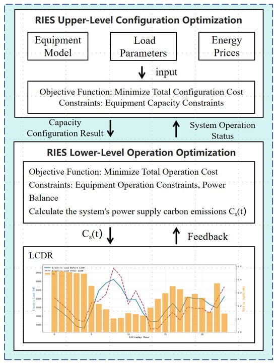
Figure 3 illustrates the coupling mechanism among equipment capacity planning, system operation, and low-carbon demand response (LCDR). The proposed approach is formulated as a two-layer optimization framework for capacity configuration and operation. Based on the fundamental equipment models, the objective functions and constraints are established using building load data, energy prices, and equipment costs as input parameters. This framework comprehensively coordinates electricity purchasing, local generation, energy conversion, energy storage, and inter-regional electricity and heat exchanges to satisfy electricity, heating, and cooling demands, thereby balancing investment costs and operational requirements.

Figure 3. Flow chart of RIES capacity configuration and operational optimization.

As shown in Figure 3, a preliminary operational optimization is first conducted without building load participation in demand response. Based on these preliminary operational results, the dynamic electricity supply carbon emission responsibility factor (Cs), which reflects the real-time carbon intensity of the system’s electricity supply, is calculated synchronously. Subsequently, Cs is fed back into the model as a dynamic carbon signal. This signal guides flexible electrical loads to shift across hours within the response constraints (i.e., building loads enter a responsive state). Under these conditions, the load data after LCDR are fed back into the optimization model to further optimize system operation. Finally, the system optimization results are obtained when building loads participate in LCDR.

The optimization model constructed in this paper is a mixed-integer linear programming (MILP) model that is solved using the Gurobi 12.0.2 solver. Before solving the model, Gurobi simplifies the model using extensive preprocessing, removing redundant constraints and variables to improve solution efficiency. The model solution adopts a two-step method of “continuous relaxation–branch-and-bound.” First, the barrier method is used to solve the continuous relaxation problem of the model; then, the continuous interior point solution is converted into a vertex solution through crossover, and the branch-and-bound method is used to find the optimal integer solution. The solution results show that the model achieves the optimization objective of minimizing the total cost of the RIES while satisfying multi-energy power balance and equipment operation constraints.

5. Case Study

5.1. Parameter Setting

The additional model settings are specified as follows. The electrical storage SOC ranges from 0.1 to 0.9, while the normalized thermal storage level ranges from 0 to 1. The maximum charging and discharging rates are both 0.2 h⁻¹ for electrical storage and 0.25 h⁻¹ for thermal storage. The thermal storage capacity upper limits are 6000 kWh for RIES 1 and 5000 kWh for RIES 2. The maximum load-shifting-in and load-shifting-out proportions are both 0.1. The carbon trading price and the internal LCDR settlement price are both set to 0.08 CNY/kg CO₂. The discount rate is 8%, and the project lifetime is 20 years.

This study mainly considers the capacity configuration and operational optimization of multiple RIESs under the LCDR mechanism. To accurately reflect realistic load fluctuations and validate the optimization results, the cooling, heating, and electrical loads of various buildings involved in the calculation are derived from actual power grid operational data from a region of Japan, covering 8760 h with a 1-h time resolution and 100% data completeness.

The significant differences in the power and thermal balance results between RIES 1 and RIES 2 are primarily due to the distinct building load characteristics in each system:

(1) RIES 1 primarily comprises residential buildings and hospitals. The load profile of residential buildings exhibits a distinct dual-peak pattern (high in the morning and evening, with a lower load at midday), whereas the hospital load curve is relatively stable with a slight decrease at night.

(2) RIES 2 primarily comprises office buildings, shopping malls, and museums. The overall load of these commercial and office buildings predominantly features a daytime peak and lower loads in the morning and evening.

These inherent differences in building load profiles directly lead to distinct operational strategies and energy flow characteristics in the two systems.

The price of purchasing electrical energy from the upper-level grid is shown in Table 1, and the price of purchasing natural gas is 0.27 CNY/kWh. RIES optimization also involves various energy supply equipment, and the parameters of each piece of equipment are shown in Table 2 and Table 3.

Table 1. Electricity purchase price table.

	Time Frame	Price (CNY/kWh)
Night	22:00–6:00	0.289
Daytime	6:00–8:00, 11:00–13:00, 15:00–18:00, 21:00–22:00	0.597
Peak time	8:00–11:00, 13:00–15:00, 18:00–21:00	0.991

Table 2. Price parameters of equipment [35,36,37,38].

Equipment	CHP (CNY/kW)	PV (CNY/kW)	Gas-Fired Boiler (CNY/kW)	Absorption Chillers (CNY/kW)	Heat Pumps (CNY/kW)	TES (CNY/kWh)	ESS (CNY/kWh)
Price	4000	2000	1000	1200	3000	150	1500

Table 3. Performance parameters of various equipment [35,36,37,38].

Equipment	CHP	PV	Gas-Fired Boiler	Absorption Chillers	Heat Pumps	TES	ESS
Parameters	Efficiency: 0.45/0.40	Efficiency: 0.95	Efficiency: 0.9	COP: 1.2	COPh: 3.0 COPc: 2.8	Efficiency: 0.9 Loss: 0.04	Efficiency: 0.9 Loss: 0.01
Life	20 years

It should be noted that this case study serves as a methodological transferability study. The measured load profiles of various buildings are derived from the Kitakyushu area of Japan, which provides realistic multi-energy demand characteristics across different building types. Meanwhile, the tariff parameters, investment costs, and natural gas prices are presented in CNY, reflecting the typical Chinese power market framework (Table 1). This combination is intentional. It allows the study to validate the proposed optimization method using highly realistic physical load datasets, while evaluating its economic performance under a representative and transparent market pricing framework. Therefore, this study demonstrates the methodological transferability and applicability of the proposed approach using measured datasets across different regional contexts.

5.2. Applicability Analysis of $C_r$

The conventional carbon emission factor $C_e$ (i.e., total carbon emissions divided by total power generation at the corresponding time) is compared with $C_r$ in this paper. Assuming that the electrical load demand is completely met by purchased electricity, the annual carbon emissions on the user side calculated using $C_e$ and $C_r$ are 27.224 million tons of CO₂ and 27.229 million tons of CO₂, respectively. The total carbon emissions on the user side calculated on an annual scale are almost equal, with a small error of approximately 0.019%, which meets the consistency principle. Thus, they are comparable.

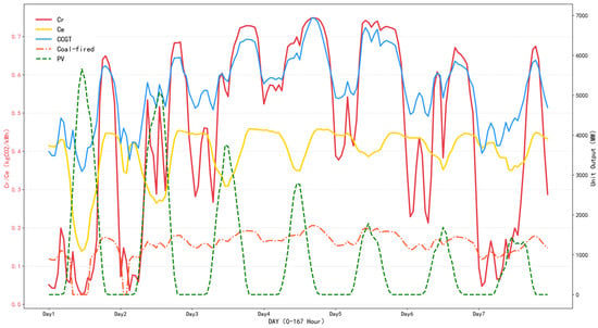
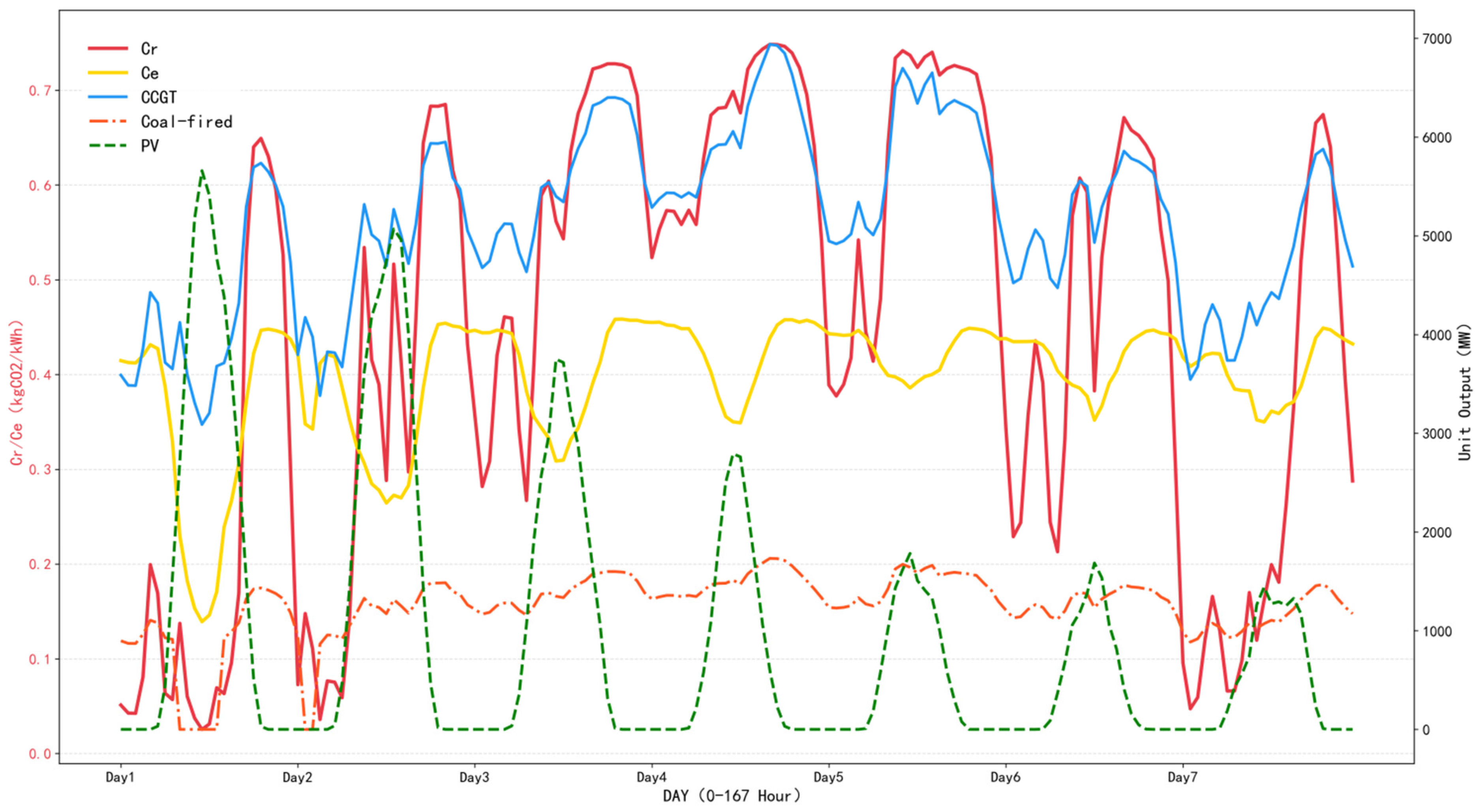
At the same time, Figure 4 shows a comparison between the two carbon indicators $C_r$ and $C_e$ and the output of each unit. Given that the output of hydropower in this region is relatively stable with little fluctuation in the output curve, and that the overall installed capacity of wind power is small with no obvious change comparison, their output curves are not displayed in Figure 4.

Figure 4. Comparison diagram of carbon indicators and unit output in a typical summer week.

$C_r$ shows better sensitivity than $C_e$. $C_e$ almost only fluctuates significantly with changes in photovoltaic output, and it is difficult to fully reflect the actual output of each thermal power unit and the supply–demand relationship of electricity. In contrast, $C_r$ fluctuates greatly with time, reflecting not only renewable energy output but also changes in the output of thermal power units. It can also capture fluctuations in marginal carbon emissions of thermal power during “peak regulation and deep peak regulation,” thereby comprehensively reflecting the output of new energy and the electricity supply–demand relationship.

Figure 5 shows the comparison of carbon emission results of load LCDR guided by $C_e$ and $C_r$, separately, on a typical summer day (assuming that the electrical load demand is completely met by purchased electricity). Under the constraint that users participate in LCDR to keep the total daily load unchanged, the LCDR using $C_r$ reduces 961 kg CO₂ per day, whereas the LCDR using $C_e$ reduces 243 kg CO₂ per day. It is evident that the LCDR using $C_r$ has higher carbon reduction benefits; thus, the use of $C_r$ can better stimulate loads to participate in LCDR.

Figure 5. Comparison diagram of carbon emission results of LCDR guided by $C_e$ and $C_r$ on a typical summer day.

The above analysis shows that during periods when electricity is exclusively purchased from the external power grid, LCDR using $C_r$ has higher sensitivity and provides stronger incentive for loads to participate in LCDR.

5.3. Sensitivity Analysis of $C_{e,t}^{cchp}$

Figure 6 illustrates the intraday variation in ${\mathrm{C}}_{\mathrm{e},\mathrm{t}}^{\mathrm{c}\mathrm{c}\mathrm{h}\mathrm{p}}$. Here, ${\mathrm{C}}_{\mathrm{e},\mathrm{t}}^{\mathrm{c}\mathrm{c}\mathrm{h}\mathrm{p}}$ exhibits pronounced fluctuations in response to changes in the “heat surplus ratio” and “heat deficit ratio” of the CHP unit, with values ranging from 0.08 to 0.38 kg CO2/kWh. The daily maximum values is approximately five times the minimum value. These results indicate that the proposed dynamic carbon emission responsibility factor for CHP electricity supply, ${\mathrm{C}}_{\mathrm{e},\mathrm{t}}^{\mathrm{c}\mathrm{c}\mathrm{h}\mathrm{p}}$, exhibits sufficient sensitivity to effectively incentivize demand response.

Figure 6. Fluctuation in ${\mathrm{C}}_{\mathrm{e},t}^{\mathrm{c}\mathrm{c}\mathrm{h}\mathrm{p}}$.

5.4. Analysis of Optimization Results

5.4.1. Comparative Scenario Settings

To verify the economic and low-carbon performance of the proposed optimization method for multi-RIES considering LCDR, three scenarios are established for comparison, as follows:

Case 1: Two RIESs operate in an interconnected manner with energy interaction but without load participation in LCDR;

Case 2: Two RIESs operate in an interconnected manner with energy interaction with load participation in LCDR;

Case 3: Two RIESs operate independently without energy interaction and consider load participation in LCDR.

The three scenarios are designed to compare the impact of the LCDR mechanism driven by $C_s$ on the system configuration and operational optimization of interconnected systems by comparing Case 1 and Case 2; Case 2 and Case 3 are used to compare the differences between independent and interconnected system operation under the LCDR mechanism.

5.4.2. Analysis of LCDR Results Based on ${\mathrm{C}}_{\mathrm{s}}$

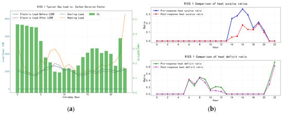
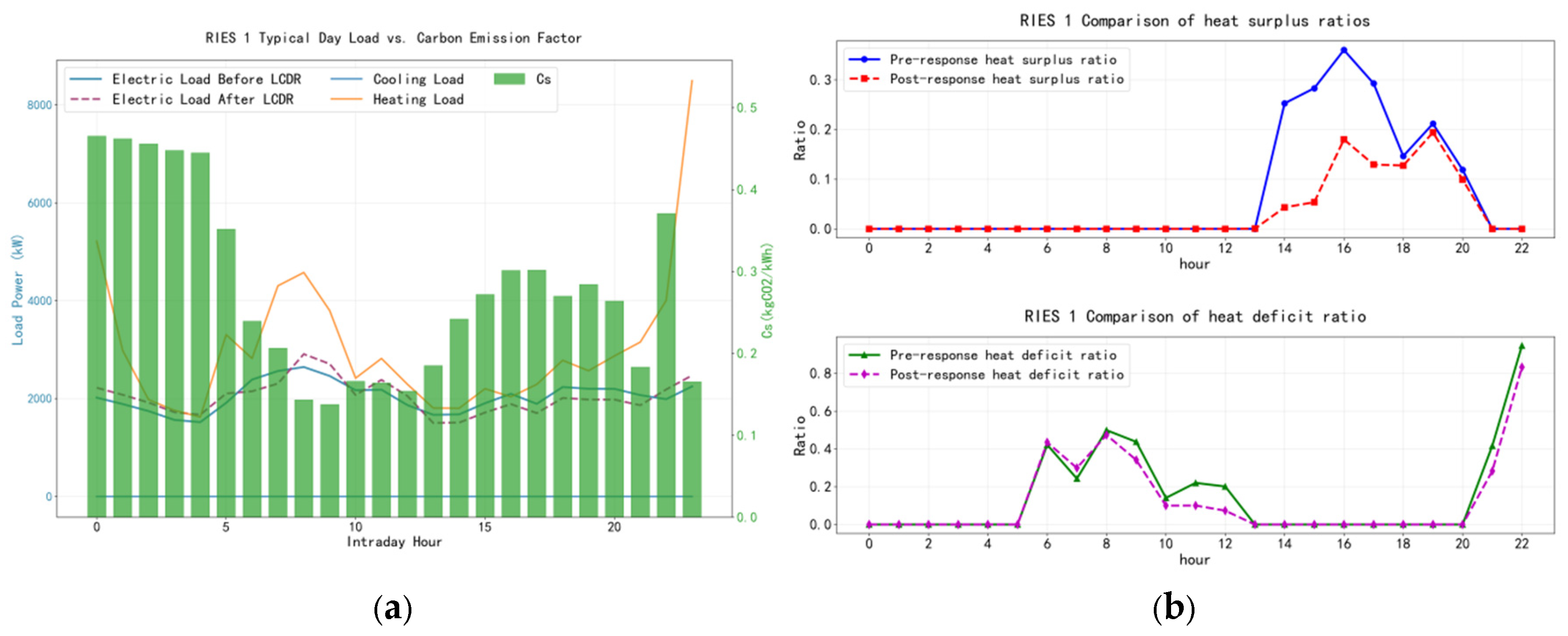
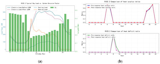
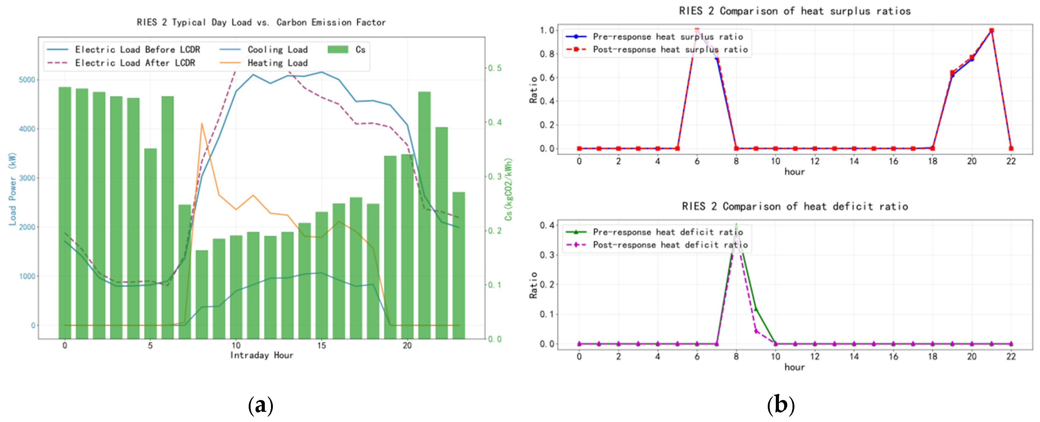
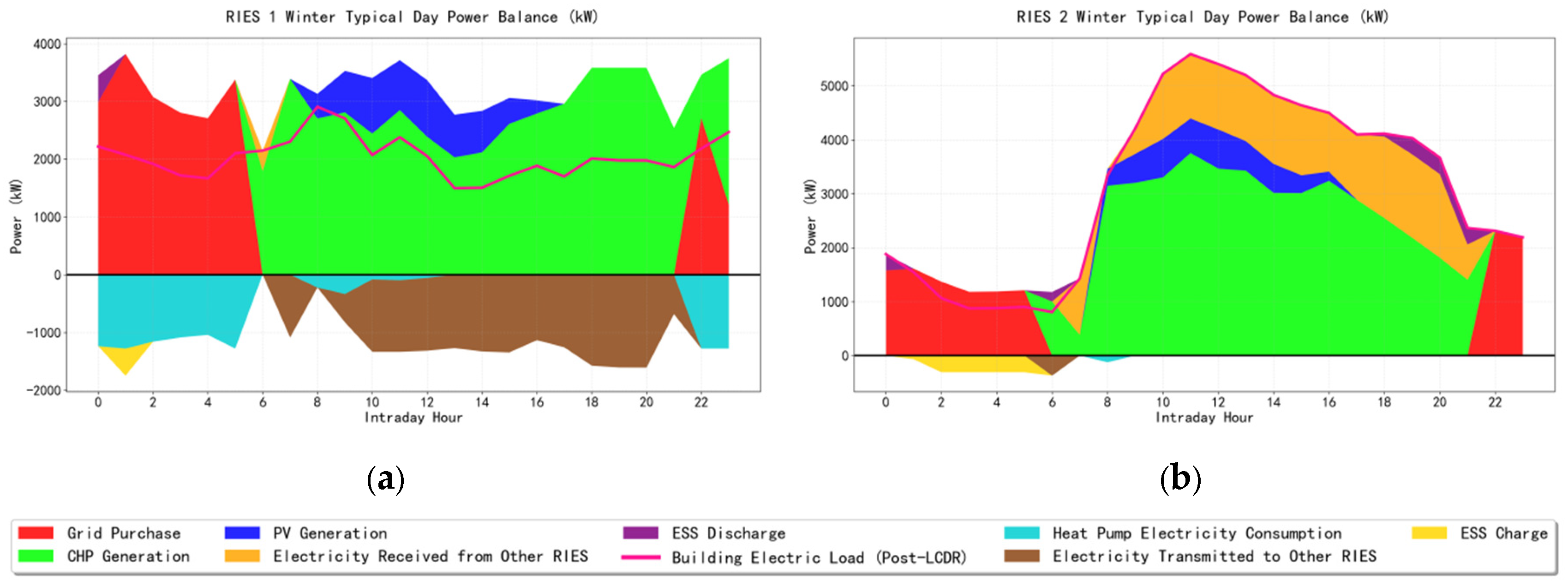
Taking the winter heating period in Case 2 as an example, the RIES features multiple energy supply sources, and different supply strategies lead to variations in the electricity supply carbon emission responsibility factor ${\mathrm{C}}_{\mathrm{s}}$. As shown in Figure 7a and Figure 8a, the values of ${\mathrm{C}}_{\mathrm{s}}$ are relatively high during the periods 0:00–5:00 and 22:00–24:00. This is because electricity prices are low during these hours, making electricity purchases from the external grid more economically attractive while the CHP units are not in operation (as illustrated in Figure 9). Under these conditions, ${\mathrm{C}}_{\mathrm{s}}$ is equal to ${\mathrm{C}}_{\mathrm{r}}$. During the period from 6:00 to 21:00, when photovoltaic generation is available and the CHP units experience a heat deficit, the values of ${\mathrm{C}}_{\mathrm{s}}$ are relatively low. In contrast, when a heat surplus occurs in the CHP units, ${\mathrm{C}}_{\mathrm{s}}$ increases accordingly. The heat surplus ratio and heat deficit ratio of the CHP units during different time periods are shown in Figure 7b and Figure 8b.

Figure 7. Comprehensive comparison diagram of typical daily loads and $C_s$ of RIES 1. (a) Typical daily electrical, heating, and cooling loads and the electricity supply carbon responsibility factor; (b) CHP heat surplus and heat deficit ratios before and after LCDR.

Figure 8. Comprehensive comparison diagram of typical daily loads and $C_s$ of RIES 2. (a) Typical daily electrical, heating, and cooling loads and the electricity supply carbon responsibility factor; (b) CHP heat surplus and heat deficit ratios before and after LCDR.

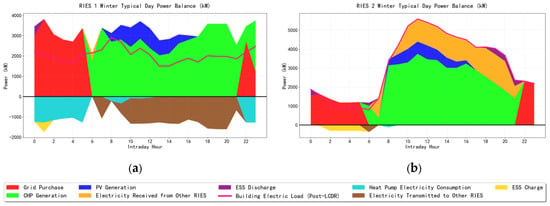
Figure 9. Electrical power balance diagram on a typical winter day. (a) RIES 1; (b) RIES 2.

Compared with Case 1, the electrical load in Case 2, through participation in low-carbon demand response (LCDR), effectively improves the matching between electricity and heat load profiles and enhances the energy utilization efficiency of the CHP units. In RIES 1, which mainly supplies residential and hospital buildings, LCDR participation reduces the average “heat surplus ratio” of the CHP units by 9%, with a maximum reduction of 19.7%, whereas the average “heat deficit ratio” decreases by 6%, with a maximum reduction of 18%. As a result, the annual CO₂ emissions of RIES 1 are reduced by 32 tons.

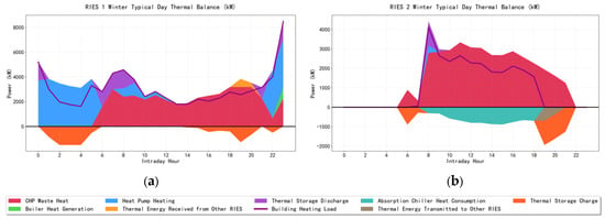
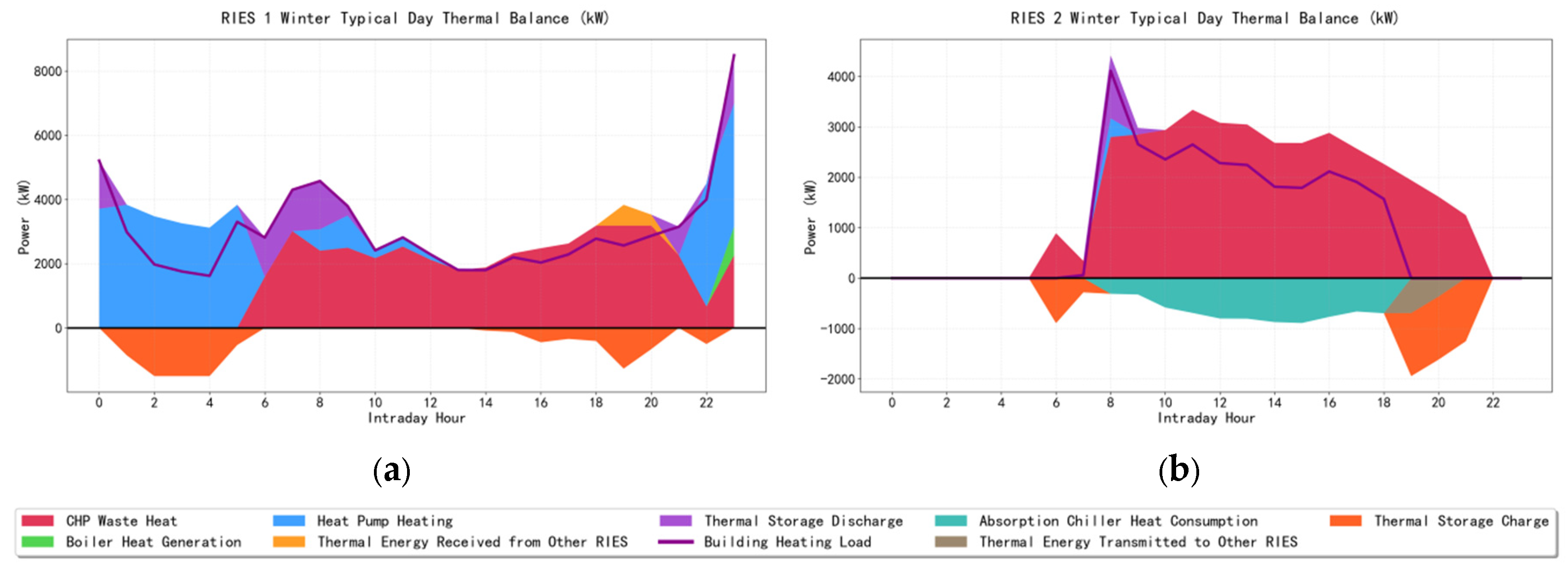
In contrast, RIES 2 primarily serves office buildings, where the electricity and heat load profiles exhibit better inherent matching. Consequently, the values of ${\mathrm{C}}_{\mathrm{s}}$ in RIES 2 are more strongly influenced by photovoltaic (PV) generation. After LCDR implementation, the peak electrical load shifts closer to periods of high PV output (as shown in Figure 9b), thereby reducing the demand for thermal power generation during peak load periods. This leads to an annual CO₂ emission reduction of 300 tons in RIES 2. As illustrated in Figure 10b, during the periods 6:00–7:00 and 19:00–21:00, heat demand in RIES 2 is either absent or relatively low. According to Equation (36), the potential for optimizing the CHP heat surplus ratio during these periods is therefore limited, which is consistent with the results shown in Figure 8b.

Figure 10. Thermal power balance diagram on a typical winter day. (a) RIES 1; (b) RIES 2.

The above analysis shows that participation in LCDR effectively improves the matching between electricity and heat loads, enhances overall system energy utilization efficiency, and provides a positive incentive for carbon emission reduction.

5.4.3. Analysis of Equipment Capacity Optimization Results

Simulation-based optimization is conducted using hourly load data over the entire year, and the resulting equipment capacities under different scenarios are summarized in Table 4. Compared with Case 1, Case 2, which incorporates low-carbon demand response, exhibits more pronounced changes in photovoltaic (PV) and electrical energy storage capacities. Under the low-carbon demand response mechanism, electrical loads are shifted from high-carbon periods to low-carbon periods, and the post-response load peaks are aligned more closely with periods of high PV generation. This reduces the demand for thermal power generation during peak electricity consumption periods and leads to an overall increase of 15.1% in installed PV capacity.

Table 4. Equipment capacity configuration results of RIESs under different scenarios.

	RIES	CHP (kW)	Absorption Chillers (kW)	Gas-Fired Boiler (kW)	Heat Pumps (kW)	PV (kW)	ESS (kWh)	TES (kWh)
Case 1	1	3668	7328	2812	3847	5246	0	6000
	2	5628	17,825	6649	905	4980	4032	5000
Case 2	1	3585	7338	2892	3837	6762	2336	6000
	2	5527	17,808	6726	922	5006	1527	5000
Case 3	1	3037	6999	8901	4176	5366	0	6000
	2	5050	8456	1308	10,274	7323	7131	5000

With respect to electrical energy storage, the substantial increase in PV capacity in RIES 1 results in surplus PV generation during summer peak periods. Consequently, additional electrical energy storage capacity is installed to store excess PV electricity. In contrast, although PV capacity in RIES 2 increases slightly, the improved alignment between the electrical load profile and PV generation after demand response reduces surplus PV output during peak generation periods, leading to a decrease in the required electrical energy storage capacity.

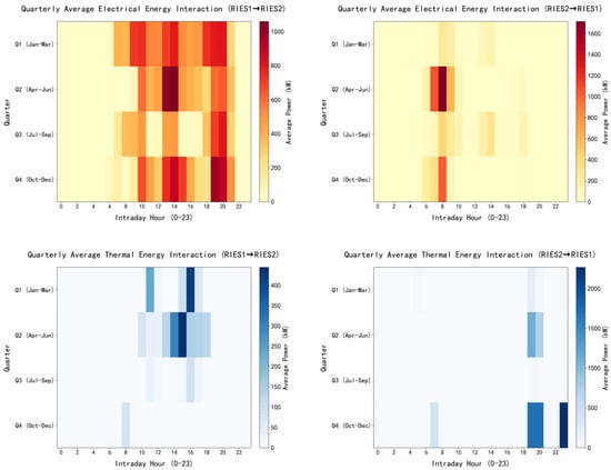
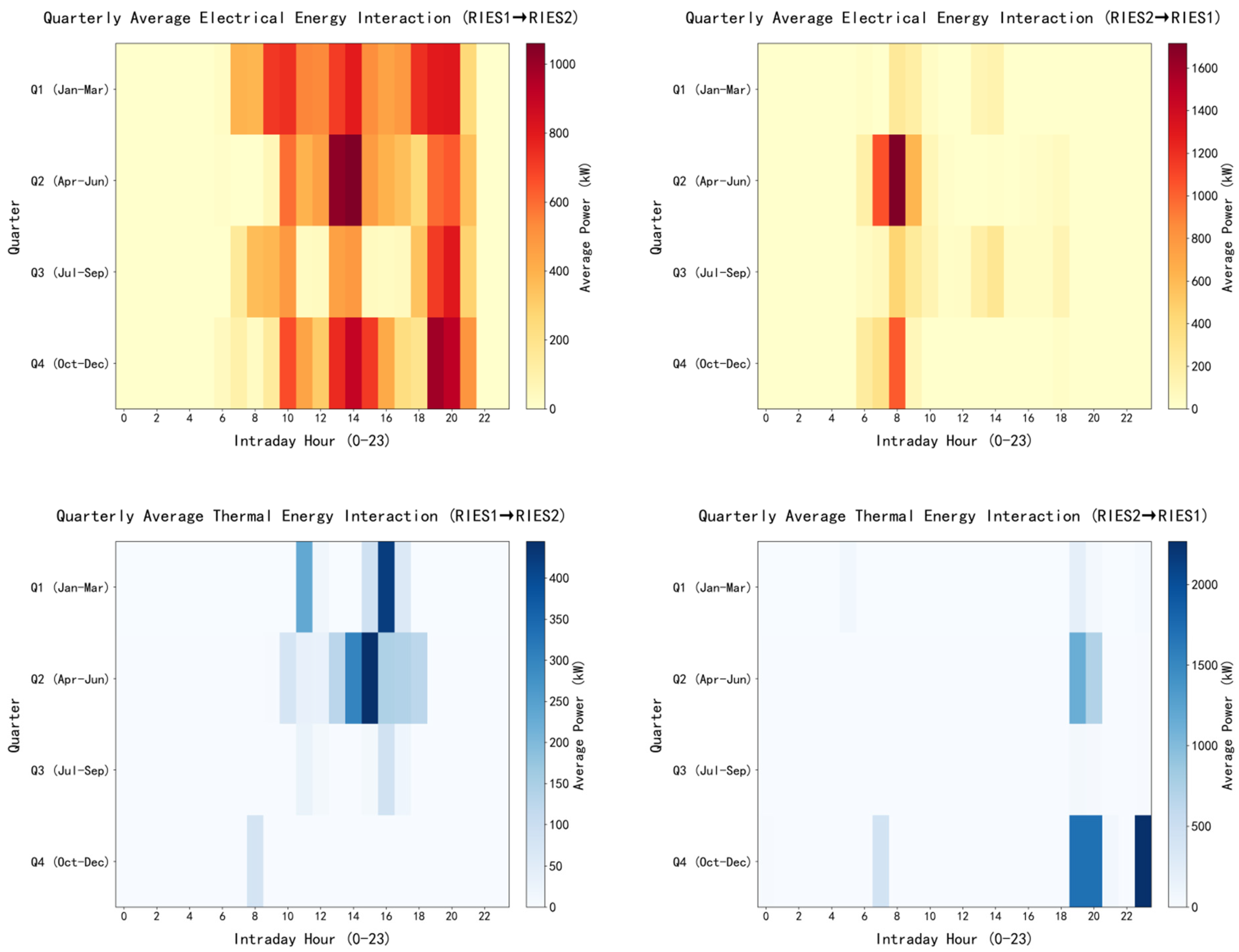
Compared with Case 3, Case 2 allows energy exchanges between different RIESs. Figure 11 illustrates the average hourly inter-regional energy exchanges across different seasons. Under the interconnected operating mode, differences in load characteristics across regions enable RIES 1 to fully exploit the heating capability of its CHP units. Because the surplus electricity generated during CHP heat production can be transmitted through the interconnection network and absorbed by RIES 2 (as shown in Figure 9 and Figure 10), RIES 1 is no longer constrained by local electricity absorption limitations when operating the CHP units. Consequently, the reliance on gas boilers for supplementary heating is substantially reduced, leading to a significant decrease in redundant gas boiler capacity. For RIES 2, during the second quarter (the cooling season), a considerable amount of surplus heat from RIES 1 is transferred to supply cooling (as shown in Figure 11). As a result, the capacity of absorption chillers in RIES 2 is increased, while the capacity of higher-cost heat pumps is reduced. The reduction in heat pump capacity lowers heating capability, which subsequently necessitates an increase in gas boiler capacity. Overall, the equipment configuration of the system is effectively optimized.

Figure 11. Heatmap of energy interaction between RIESs in different quarters.

5.4.4. Analysis of System Economic Cost Optimization Results

To provide a clear comparison, the optimization results are analyzed based on two distinct baselines:

• Impact of LCDR (Case 2 vs. Case 1):

Comparing Case 2 with Case 1 isolates the effect of LCDR. The introduction of LCDR guided by ${\mathrm{C}}_{\mathrm{s}}$ reduces the annual total system cost by 0.55 million CNY and CO₂ emissions by 333.2 tons (approximately 1.4%). The increase in installed PV capacity reduces the demand for thermal power generation. Although the total investment cost rises slightly, the operational cost is significantly reduced, with electricity purchases from the external grid decreasing by 556.4 MWh and natural gas consumption decreasing by 1004.9 MWh. Overall, LCDR effectively lowers system carbon emissions, improves economic performance, and reduces dependence on external energy supplies.

2.

Impact of interconnection and trade-off analysis (Case 2 vs. Case 3):

Comparing Case 2 with Case 3 isolates the effect of multi-regional interconnection. The annual total system cost in Case 2 is reduced by 1.948 million CNY (approximately 4.1%), and electricity purchases from the external grid decrease by 4914.5 MWh (approximately 18.2%). Under the interconnected operating mode, complementary exchanges of electricity and heat among RIESs reduce equipment redundancy, significantly lowering investment costs.

It should be emphasized that the moderate increase in CO₂ emissions in Case 2 compared to Case 3 is not a drawback but a reasonable trade-off for economic efficiency and system autonomy. This increase is mainly attributed to the reduced electricity purchases from the external grid, which leads to greater reliance on local energy supply and higher natural gas consumption. However, the increased total output of CHP units results in higher allocated carbon allowances, thereby reducing carbon trading costs (164,000 CNY in Case 2 vs. 314,000 CNY in Case 3). Overall, while independently operated systems (Case 3) exhibit lower carbon emissions, they suffer from higher total costs and stronger dependence on external energy networks. In contrast, the interconnected system (Case 2) demonstrates superior economic performance, stronger autonomy, and enhanced operational stability.

3.

Comprehensive benefit evaluation:

To quantitatively balance the trade-off between economic and low-carbon aspects, the CBI values for the three cases under different weights are calculated based on Table 5 and Table 6, as shown in Table 7. Under equal weights (ω1 = 0.5, ω2 = 0.5), Case 3 achieves the lowest CBI due to its superiority in total carbon emissions. However, considering that ensuring economic viability is the primary concern for system operators, this study assigns slightly higher weights to the economic index (ω1 = 0.6, ω2 = 0.4 and ω1 = 0.7, ω2 = 0.3). Under both practical weight settings, Case 2 achieves the lowest CBI, demonstrating the optimal comprehensive performance and effectively balancing operational costs with carbon reduction. This proves that the proposed coordinated optimization strategy (Case 2) is a robust and practical solution.

Table 5. Economic costs of each RIES under different scenarios (10,000 CNY).

	RIES	Annual Operating Cost	Annualized Investment Cost	Annual Total Cost	Grand Total
Case 1	1	1327.4	504.5	1831.9	4557.5
	2	2009.2	716.4	2725.6
Case 2	1	1311.7	568.2	1879.9	4502.5
	2	1947.0	675.6	2622.6
Case 3	1	1265.7	546.0	1811.7	4697.3
	2	1983.5	902.1	2885.6

Table 6. Energy purchase and carbon emission status of each RIES under different scenarios.

	RIES	Electricity Purchase (MWh)	Gas Purchase (MWh)	Carbon Emissions (tCO2)	Total Carbon Emissions (tCO2)
Case 1	1	9340.8	31,915.8	9691.3	23,383.0
	2	13,326.5	45,453.2	13,691.7
Case 2	1	9643.8	31,239.1	9658.4	23,049.8
	2	12,467.1	45,125.0	13,391.4
Case 3	1	10,470.5	26,985.3	9006.4	21,854.1
	2	16,554.9	37,308.7	12,847.7

Table 7. CBI values for the three cases under different weights.

	${\mathsf{\omega }}_1=0.7$ ${\mathsf{\omega }}_2=0.3$	${\mathsf{\omega }}_1=0.6$ ${\mathsf{\omega }}_2=0.4$	${\mathsf{\omega }}_1=0.5$ ${\mathsf{\omega }}_2=0.5$
CBI1 (Baseline)	1.0000	1.0000	1.0000
CBI2	0.9873	0.9871	0.9868
CBI3	1.0019	0.9923	0.9826

5.4.5. Literature-Based Qualitative Comparison of Key Parameters

Based on the established literature, the impacts of key parameters on system operation are analyzed as follows. Regarding carbon pricing, policies such as the ladder-type carbon trading scheme raise the emission cost of high-carbon units, directly incentivizing the system to reduce fossil fuel generation and lower total carbon emissions [39]. However, the system’s response to carbon pricing is non-linear, with specific sensitive and insensitive intervals resulting in a stepwise cost curve [40], and a specific threshold is required to optimally balance economic costs and emission reductions without diminishing marginal returns [41]. For electricity prices, system costs are highly sensitive to fluctuations [42]; higher electricity prices strengthen the economic incentive for demand response, driving stronger load shifting. When aligned with carbon prices, this can create a synergistic incentive to further promote low-carbon operations [43,44]. Regarding load and PV output uncertainty, these factors primarily alter the low-carbon periods and the charging/discharging cycles of energy storage [45], thereby affecting the actual operational scheduling of the system. This highlights robust or stochastic optimization under uncertainty as a crucial direction for future work.

6. Conclusions and Prospects

In this study, we investigated the capacity planning and operational optimization of multi-regional integrated energy systems (RIESs) considering low-carbon demand response. A low-carbon guidance mechanism centered on the dynamic carbon emission responsibility factor for electricity supply, $C_s$, is developed and integrated with economic models for equipment capacity configuration and system operation, enabling coordinated optimization of economic performance and carbon reduction. Simulation studies based on real load and generation data from a region in Japan verify the effectiveness and practicality of the proposed method. The main conclusions are summarized as follows:

(1)

A dynamic low-carbon guidance signal suitable for RIESs is proposed. By introducing the carbon emission responsibility factor for externally purchased electricity, $C_r$, and decoupling the electricity–heat coupling characteristics of CHP units, a dynamic carbon emission responsibility allocation mechanism based on the CHP electricity-side weighting factor ${\omega }_{e,t}$ is established. By further incorporating photovoltaic generation and inter-regional energy interactions, a dynamic electricity supply carbon emission responsibility factor for RIES, $C_s$, is constructed to accurately reflect the electricity carbon intensity under different operating strategies in real time.

(2)

Under the low-carbon demand response mechanism guided by $C_s$, electrical loads actively shift toward low-carbon periods, effectively improving the matching between electricity and heat load profiles and aligning peak electricity demand more closely with photovoltaic generation periods. This mechanism significantly enhances the energy utilization efficiency of CHP units and the utilization of photovoltaic energy, thereby effectively reducing overall system carbon emissions.

(3)

The coordinated optimization of multi-regional interconnection and low-carbon demand response significantly improves the overall operational performance of the system. Compared with interconnected operation without low-carbon demand response, the introduction of low-carbon demand response reduces both system operating costs and carbon emissions. Compared with single-region independent operation, multi-regional interconnection optimizes equipment configuration through complementary exchanges of electricity and heat, reduces reliance on external energy supplies, and markedly enhances system autonomy and operational stability. These distinct effects indicate that regional energy sustainability should be evaluated against explicit baselines, accounting for both economic performance and operational carbon emissions.

Future work may further consider incorporating new energy elements such as hydrogen to enrich multi-energy complementarity forms and introduce robust optimization or stochastic optimization methods to improve model robustness by accounting for uncertainties in wind and solar output and load demand.

References

- IEA. World Energy Outlook 2023; International Energy Agency: Paris, France, 2023. [Google Scholar]
- IPCC. Climate Change 2022: Mitigation of Climate Change; Cambridge University Press: Cambridge, UK, 2022. [Google Scholar]
- Mancarella, P. MES (multi-energy systems): An overview of concepts and evaluation models. Energy 2014, 65, 1–17. [Google Scholar] [CrossRef] [Scilit]
- Gao, X.; Xiao, H.; Xu, S.; Lin, H.C.; Chang, P. What Is the Optimal Solution for Scheduling Multiple Energy Systems? Overview and Analysis of Integrated Energy Co-Dispatch Models. Energies 2024, 17, 4718. [Google Scholar] [CrossRef] [Scilit]
- Cheng, H.; Hu, X.; Wang, L.; Liu, Y.; Yu, Q. Review on research of regional integrated energy system planning. Autom. Electr. Power Syst. 2019, 43, 2–13. (In Chinese) [Google Scholar]
- Lin, X.; Zhang, N.; Zhong, W.; Kong, F.; Cong, F. Regional integrated energy system long-term planning optimization based on multi-energy complementarity quantification. J. Build. Eng. 2023, 68, 106046. [Google Scholar] [CrossRef] [Scilit]
- Jia, H.; Wang, D.; Xu, X.; Yu, X. Research on some key problems related to integrated energy systems. Autom. Electr. Power Syst. 2015, 39, 198–207. (In Chinese) [Google Scholar]
- Geidl, M.; Andersson, G. Optimal power flow of multiple energy carriers. IEEE Trans. Power Syst. 2007, 22, 145–155. [Google Scholar] [CrossRef] [Scilit]
- Zhang, X.; Shahidehpour, M.; Alabdulwahab, A.; Abusorrah, A. Optimal expansion planning of energy hub with multiple energy infrastructures. IEEE Trans. Smart Grid 2015, 6, 2302–2311. [Google Scholar] [CrossRef] [Scilit]
- Gabrielli, P.; Gazzani, M.; Martelli, E.; Mazzotti, M. Optimal design of multi-energy systems with seasonal storage. Appl. Energy 2018, 219, 408–424. [Google Scholar] [CrossRef] [Scilit]
- Yang, C.; You, S.; Han, Y.; Wang, X.; Li, J.; Wang, L. Research on Optimization Method of Integrated Energy System Network Planning. Sustainability 2023, 15, 8843. [Google Scholar] [CrossRef] [Scilit]
- Zheng, W.; Zou, B.; Gu, J.; Chen, J.; Hou, J. Study on optimal allocation of energy storage in multi-regional integrated energy system considering stepped carbon trading. Int. J. Low-Carbon Technol. 2024, 19, 551–558. [Google Scholar] [CrossRef] [Scilit]
- Li, Q.; Wang, J.; Chen, J.; Ding, T.; Gu, C. A hierarchical multi-area capacity planning model considering configuration ratios of renewable energy and energy storage systems with multi-area coordination. IET Gener. Transm. Distrib. 2023, 17, 3658–3677. [Google Scholar] [CrossRef] [Scilit]
- Zhou, B.; Li, E. Multi-Regional Integrated Energy Economic Dispatch Considering Renewable Energy Uncertainty and Electric Vehicle Charging Demand Based on Dynamic Robust Optimization. Energies 2024, 17, 2453. [Google Scholar] [CrossRef] [Scilit]
- Palensky, P.; Dietrich, D. Demand side management: Demand response, intelligent energy systems, and smart loads. IEEE Trans. Ind. Inform. 2011, 7, 381–388. [Google Scholar] [CrossRef] [Scilit]
- Song, Y.; Mu, H.; Li, N.; Wang, H.; Kong, X. Optimal scheduling of zero-carbon integrated energy system considering long- and short-term energy storages, demand response, and uncertainty. J. Clean. Prod. 2024, 435, 140393. [Google Scholar] [CrossRef] [Scilit]
- Zhu, B.; Wang, D. Master–Slave Game Optimal Scheduling for Multi-Agent Integrated Energy System Based on Uncertainty and Demand Response. Sustainability 2024, 16, 3182. [Google Scholar] [CrossRef] [Scilit]
- Choi, W.; Im, J.; Lee, J.; Chung, J.H.; Lee, D. Operating strategy for load service entities using flexible real-time pricing through stochastic dual dynamic programming. Sci. Rep. 2025, 15, 33576. [Google Scholar] [CrossRef] [Scilit]
- Hu, B.; Zong, X.; Wu, H.; Yang, Y. Distributed Low-Carbon Demand Response in Distribution Networks Incorporating Day-Ahead and Intraday Flexibilities. Processes 2025, 13, 2460. [Google Scholar] [CrossRef] [Scilit]
- Hong, J.; Zhang, L.; Hu, Z.; Lin, W.; Zou, Y. A robust system model for the photovoltaic in industrial parks considering photovoltaic uncertainties and low-carbon demand response. Front. Energy Res. 2024, 12, 1343309. [Google Scholar] [CrossRef] [Scilit]
- Gao, H.; Yin, B.; He, S.; Liu, J. A distributionally robust-based information gap decision theory optimization method for energy station considering low-carbon demand response. Sustain. Energy Technol. Assess. 2025, 73, 104129. [Google Scholar] [CrossRef] [Scilit]
- Fleschutz, M.; Bohlayer, M.; Braun, M.; Henze, G.; Murphy, M.D. The effect of price-based demand response on carbon emissions in European electricity markets: The importance of adequate carbon prices. Appl. Energy 2021, 295, 117040. [Google Scholar] [CrossRef] [Scilit]
- Liu, Y.; Wang, X.; Li, S.; Liu, L.; Zhao, Y.; Yu, M. Demand Response Model of Low-Carbon Economy in Integrated Energy System Based on Carbon Flow Traceability. Eng. Rep. 2025, 7, e70097. [Google Scholar] [CrossRef] [Scilit]
- Ma, F.; Ying, L.; Cui, X.; Yu, Q. Research on a Low-Carbon Optimization Strategy for Regional Power Grids Considering a Dual Demand Response of Electricity and Carbon. Sustainability 2024, 16, 7000. [Google Scholar] [CrossRef] [Scilit]
- Zhang, Y.; Sun, P.; Ji, X.; Yang, M.; Ye, P. Low-Carbon Economic Dispatch of Integrated Energy Systems Considering Full-Process Carbon Emission Tracking and Low Carbon Demand Response. IEEE Trans. Netw. Sci. Eng. 2024, 11, 5417–5431. [Google Scholar] [CrossRef] [Scilit]
- Huang, J.; Yuan, M.; Zou, Z.; Sun, Y. Low-carbon economic optimization scheduling in distributed energy systems considering carbon emission responsibility and demand response. Int. J. Electr. Power Energy Syst. 2025, 169, 110768. [Google Scholar] [CrossRef] [Scilit]
- Su, X.; Zhang, Q.; Lu, Y.; Hao, R.; Qin, T.; Li, C.; Huang, S.; Bi, K. Study on multi-energy scheduling strategy considering dynamic energy prices and low-carbon demand response. Renew. Energy 2025, 247, 123048. [Google Scholar] [CrossRef] [Scilit]
- Zhou, T.; Kang, C.; Xu, Q.; Chen, Q. Preliminary theoretical investigation on power system carbon emission flow. Autom. Electr. Power Syst. 2012, 36, 38–43, 85. (In Chinese) [Google Scholar]
- Zhou, T.; Kang, C.; Xu, Q.; Chen, Q. Preliminary investigation on a method for carbon emission flow calculation of power system. Autom. Electr. Power Syst. 2012, 36, 44–49. (In Chinese) [Google Scholar]
- Jiang, Y.; Zhang, J.; Zhang, T.; Liu, X.; Xue, Z.; Liu, Y.; Shi, J. Dynamic Carbon Emission Responsibility Factor of Electricity. Proc. CSEE 2024, 44, 7024–7039. (In Chinese) [Google Scholar]
- Guo, J.; Liu, Z.; Wu, X.; Wu, D.; Zhang, S.; Yang, X.; Ge, H.; Zhang, P. Two-layer co-optimization method for a distributed energy system combining multiple energy storages. Appl. Energy 2022, 322, 119486. [Google Scholar] [CrossRef] [Scilit]
- Li, Y.; Liu, J.; Ma, S.; Hu, Y. Source-load interactive multi-objective optimal dispatching of integrated energy system based on off-design model. Power Syst. Technol. 2022, 46, 2472–2482. (In Chinese) [Google Scholar]
- Wouters, C.; Fraga, E.S.; James, A.M. An energy integrated, multi-microgrid, MILP (mixed-integer linear programming) approach for residential distributed energy system planning–A South Australian case-study. Energy 2015, 85, 30–44. [Google Scholar] [CrossRef] [Scilit]
- Li, M.; Yang, Y.; Smith, T.M.; Wilson, E.J. Wind can reduce storage-induced emissions at grid scales. Appl. Energy 2020, 276, 115420. [Google Scholar] [CrossRef] [Scilit]
- Liu, G.; Zeng, J.; Wu, Y.; Liao, S. Multi-criteria techno-economic analysis of solar photovoltaic/wind hybrid power systems under temperate continental climate. IET Renew. Power Gener. 2022, 16, 3058–3070. [Google Scholar] [CrossRef] [Scilit]
- Liu, H.; Shen, W.; He, X.; Zeng, B.; Liu, Y.; Zeng, M.; Zhao, C. Multi-scenario comprehensive benefit evaluation model of a multi-energy micro-grid based on the matter-element extension model. Energy Sci. Eng. 2021, 9, 402–416. [Google Scholar] [CrossRef] [Scilit]
- Li, S.; Zhu, Y.; Xu, Y.; Zhou, X.; Fu, Z.; Wu, J.; Han, R.; Cheng, L.; Zhang, H.; Chen, H. Three-objective optimization and emergy analysis of integrated energy system under time-of-use flexible operation strategy. Energy Storage Sci. Technol. 2025, 14, 3447–3462. [Google Scholar] [CrossRef]
- Wang, W.; Xu, X.; Li, S.; Li, B.; Hao, J. Bi-Level Optimal Configuration of Multi-Building Flexible Interconnected Energy Systems Considering Multi-Energy Complementarity. Clean Energy Sustain. 2026, 4, 10002. [Google Scholar] [CrossRef] [Scilit]
- Zhang, C.; Qi, Y.; Cao, X.; Zhang, Y. Low-Carbon Economic Dispatch of an Integrated Energy System with Multi-Device Coupling under Ladder-Type Carbon Trading. Energy Eng. 2026, 123, 12. [Google Scholar] [CrossRef] [Scilit]
- Liao, W.; Liu, D.; Wu, Y.; Liu, T. Bi-level optimization of multi-regional power system considering low-carbon oriented synergy of both source and load sides. IET Renew. Power Gener. 2024, 18, 515–528. [Google Scholar] [CrossRef] [Scilit]
- Ren, F.; Cao, X. Optimal operation of integrated energy system with carbon capture and demand response. Appl. Therm. Eng. 2025, 280, 128216. [Google Scholar] [CrossRef] [Scilit]
- Yu, J.; Chen, L.; Wang, Q.; Zhang, X.; Sun, Q. Towards sustainable regional energy solutions: An optimized operational model for integrated energy systems with price-responsive planning. Energy 2024, 305, 132278. [Google Scholar] [CrossRef] [Scilit]
- Wang, X.; Jiao, Y.; Cui, B.; Zhu, H.; Wang, R. Two-Stage Optimal Operation of Integrated Energy System Considering Electricity-Heat Demand Response and Time-of-Use Energy Price. Int. J. Energy Res. 2025, 2025, 6106019. [Google Scholar] [CrossRef] [Scilit]
- Zhang, Y.; Bao, Z.; Yu, M. Digital Twin–Driven Low-Carbon and Economic Scheduling for Integrated Energy System With Learnt Energy–Carbon Coupling Constraints. Digit. Twins Appl. 2026, 3, e70037. [Google Scholar] [CrossRef] [Scilit]
- Li, Y.; Lu, Z.; Zhang, J.; Guo, X.; Li, X.; Kong, X.; Zhang, J. Low-carbon Joint Planning for Distribution Network Considering Carbon Emission Flow and Uncertainties from Photovoltaic Power Generation. CSEE J. Power Energy Syst. 2026, 12, 411–423. [Google Scholar] [CrossRef] [Scilit]
Disclaimer/Publisher’s Note: The statements, opinions and data contained in all publications are solely those of the individual author(s) and contributor(s) and not of MDPI and/or the editor(s). MDPI and/or the editor(s) disclaim responsibility for any injury to people or property resulting from any ideas, methods, instructions or products referred to in the content. |
© 2026 by the authors. Licensee MDPI, Basel, Switzerland. This article is an open access article distributed under the terms and conditions of the Creative Commons Attribution (CC BY) license.