Artist Mobility Networks, Hub Dependence, and Cross-Cohort Cultural Persistence: A Historical Network Analysis of Visual Artists Born in 1850–1969

Abstract

Inter-city networks of cultural producers offer one measurable window on urban cultural resilience. Using Wikidata records, with Getty ULAN identifiers for authority control, this study builds birthplace-to-work-location networks for 15,816 painters, sculptors, printmakers, and photographers born in 1850–1969 and grouped into six 20-year birth cohorts. Each tie records a documented spatial association whose timing is approximated by birth cohort. Two network-level dimensions of resilience are examined: structural dependence on hubs, through node-removal stress tests benchmarked against degree-preserving null networks, and cross-cohort persistence of cultural attraction, through historical forecasting from cohort t to cohort t + 1. In every cohort, removing the 5% of cities with the highest PageRank leaves 18–27% of the artist-flow weight, against about 90% under random removal, and every observed network is more vulnerable than its nulls. The current cultural scale carries most of the forecasting signal (held-out R² = 0.733). Connectivity adds a small, consistent increment that is clearest for identifying future hubs (ROC-AUC from 0.827 to 0.866); the regression gain (R² = 0.750) is statistically uncertain. Results hold under normalized outcomes, city-grouped validation, metropolitan harmonization, documentation controls, and event-dated ties, and the high concentration of the latest cohort reflects dense Dutch documentation.

1. Introduction

Culture occupies an uneasy position in sustainability research. It is increasingly treated as more than an instrument for economic development or social cohesion, yet its long-term viability is still less consistently operationalized than environmental, economic, or social sustainability. Work on cultural sustainability has therefore treated culture as a constituent part of sustainable development in its own right, while documenting wide variation in how the concept is defined and measured [1,2,3]. Policy discussions have moved in the same direction: UNESCO’s 2025 Global Report on Cultural Policies (updated in 2026) frames inclusive and sustainable cultural ecosystems, the protection of artists, and resilience under crisis as connected policy concerns [4].

In this paper, cultural sustainability refers to the long-run capacity of a cultural system to renew its practices, producers, and meanings across generations [1,3]. Resilience refers to how the functions of a system respond to a disturbance, whether by absorbing it, adapting, or reorganizing [5,6,7]. Persistence is narrower: the continuation of an observed property from one period to the next. Cultural attraction, in this study, is the volume of documented artist ties a city receives from other places within a birth cohort. The link to sustainability runs through circulation. Cities that keep drawing cultural producers from elsewhere retain the labor, training, and exchange through which practices are renewed, and a system whose circulation passes through a few hubs concentrates the exposure of that renewal to local disruption [8,9]. Continued production, institutional survival, and audience reach are equally relevant dimensions of cultural sustainability; they require data on outputs, organizations, and publics that a biographical source does not provide, and they remain outside the present design. Table 1 maps each concept to its working definition, its operational measure, and the sections in which it is used.

Table 1. Concepts, working definitions, and operational measures.

Concept	Working Definition in This Study	Operational Measure	Sections
Artist mobility	Documented spatial association between an artist’s birthplace and a recorded work location	Directed, fractionally weighted birthplace-to-work-location tie	Section 2.3
Cultural attraction	Documented artist ties a city receives from other places within a birth cohort	Weighted in-strength; incoming artists	Section 2.5 and Section 3.2
Structural dependence (vulnerability)	Share of network function lost when the most central cities are removed	Retained flow RF(q), largest weak component, global efficiency, average path length, modularity; z-scores against degree-preserving nulls	Section 2.6, Section 2.7, and Section 3.3
Cross-cohort persistence	Continuation of a city’s cultural attraction into the next birth cohort	Out-of-period prediction of ln(1 + in-strength) and cohort share in cohort t + 1; top-quartile hub status	Section 2.8, Section 2.9, Section 3.4, and Section 3.5
Urban cultural resilience (network dimension)	Capacity of the inter-city artist network to retain function under removal of cities and to sustain attraction across cohorts	Joint reading of structural dependence and cross-cohort persistence	Section 4
Cultural sustainability	Long-run renewal of practices and producers across generations	Context for interpretation; sustained inter-city circulation is treated as one of its conditions	Section 1 and Section 4

Artists’ careers link places of origin to places of work, forming networks through which cultural labor, knowledge, reputation, and opportunity are redistributed across cities. Planning research has long treated artists and cultural activity as spatially consequential actors [8], and mobility research shows that artists combine migration, temporary residence, repeated travel, and transnational circulation across creative cities [10]. In this study, artist mobility means a documented spatial association between an artist’s birthplace and a place where the artist is recorded as having worked. Most statements of Wikidata’s work-location property (P937) carry no date, so the data locate an artist’s professional life relative to birth, while leaving the timing, order, and number of individual moves unobserved for most artists. The networks analyzed here are therefore birthplace-to-work-location networks, and “mobility” refers to this relation throughout.

Kelly and O’Hagan used art-dictionary data on prominent Western visual artists to show strong geographic clustering of both birthplaces and later locations from the thirteenth to the twentieth century [11]. O’Hagan and Hellmanzik documented high migration rates of important visual artists toward a small number of centers [12], and Hellmanzik estimated price premiums for modern artists who worked in leading clusters such as Paris and New York [13]. Comparable patterns appear for composers [14,15]. Serafinelli and Tabellini linked the rise and decline of creative clusters in European cities to the immigration of famous people and to local institutions [16], and Borowiecki and Graddy traced how immigrant artists reshaped local artistic labor markets in the United States [17]. Together, these studies establish that artistic production concentrates in a few cities and that migration feeds this concentration, with the artist or the city as the unit of analysis. The network that connects many origin cities to many destinations and the way its structure responds when central nodes disappear have received much less attention.

Schich et al. reconstructed the movements of more than 150,000 notable individuals from their birth and death locations and traced the rise and decline of cultural centers over two millennia [18]. Cross-verified databases of notable people and curated biographical corpora have since widened the empirical base for such work [19,20]. Art historians have used quantitative and transnational evidence to question Paris-centered narratives of modernism [21], and sociologists have described the global art world as a field with multiple, unequally weighted centers [22]. Network studies of artistic careers show that early access to central institutions shapes later reputation [23,24]. At the urban scale, measurement frameworks operationalize cultural vibrancy and creative economy across European cities [25,26,27], and large-scale behavioral data show that cultural diversity varies with urban scale and interaction opportunities [28].

Complex-network research distinguishes tolerance to random failure from vulnerability to targeted attack [29], shows that the ordering used to target nodes changes the damage inflicted [30], and provides efficiency measures for networks whose paths lengthen or break under damage [31]. Regional and urban resilience research insists that the system, the function, and the time horizon under examination be specified explicitly [6,7,32]. In cultural settings, ecological and ecosystem approaches emphasize relationships, flows, and geographic scales [9,33,34,35]; creative-city debates distinguish market-led creativity from culturally and socially sustainable development [36,37]; cultural-sustainability indicators for cities have multiplied [38,39,40]; and heritage and arts places have been linked to urban resilience [41,42]. The COVID-19 pandemic exposed how quickly cultural work contracts when mobility and venues shut down [43]. Quantitative stress tests of the networks through which cultural producers circulate between cities remain rare.

Large-scale historical artist-location records have mainly been used to describe where artists were born, worked, or died; they have rarely been assembled into cohort-specific inter-city networks with fractional weights and city-level structural measures. In addition, whether such network characteristics carry prospective information about a city’s later cultural attraction, beyond its current size and its earlier prominence, has not been tested with forward-in-time validation. Finally, the dependence of these networks on central hubs has not been compared with randomized networks that preserve the observed degree structure, a comparison needed to separate hub dependence from the mechanical effect of a skewed degree distribution. These three gaps concern, respectively, the construction of historical inter-city networks, their prospective information, and their structural dependence relative to randomized benchmarks.

RQ1: How do concentration, connectivity, and source diversity vary across historical birthplace-to-work-location networks of visual artists? RQ2: Do network characteristics of cities add prospective information about their cultural attraction in the next birth cohort beyond current cultural scale and earlier prominence? RQ3: How strongly does each cohort network depend structurally on its most central cities, and does this dependence exceed that of degree-preserving randomized networks?

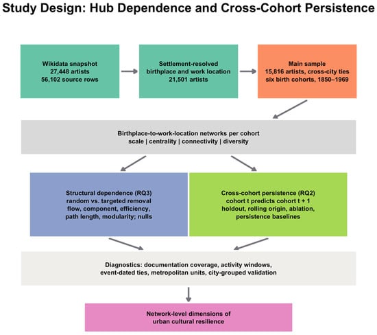
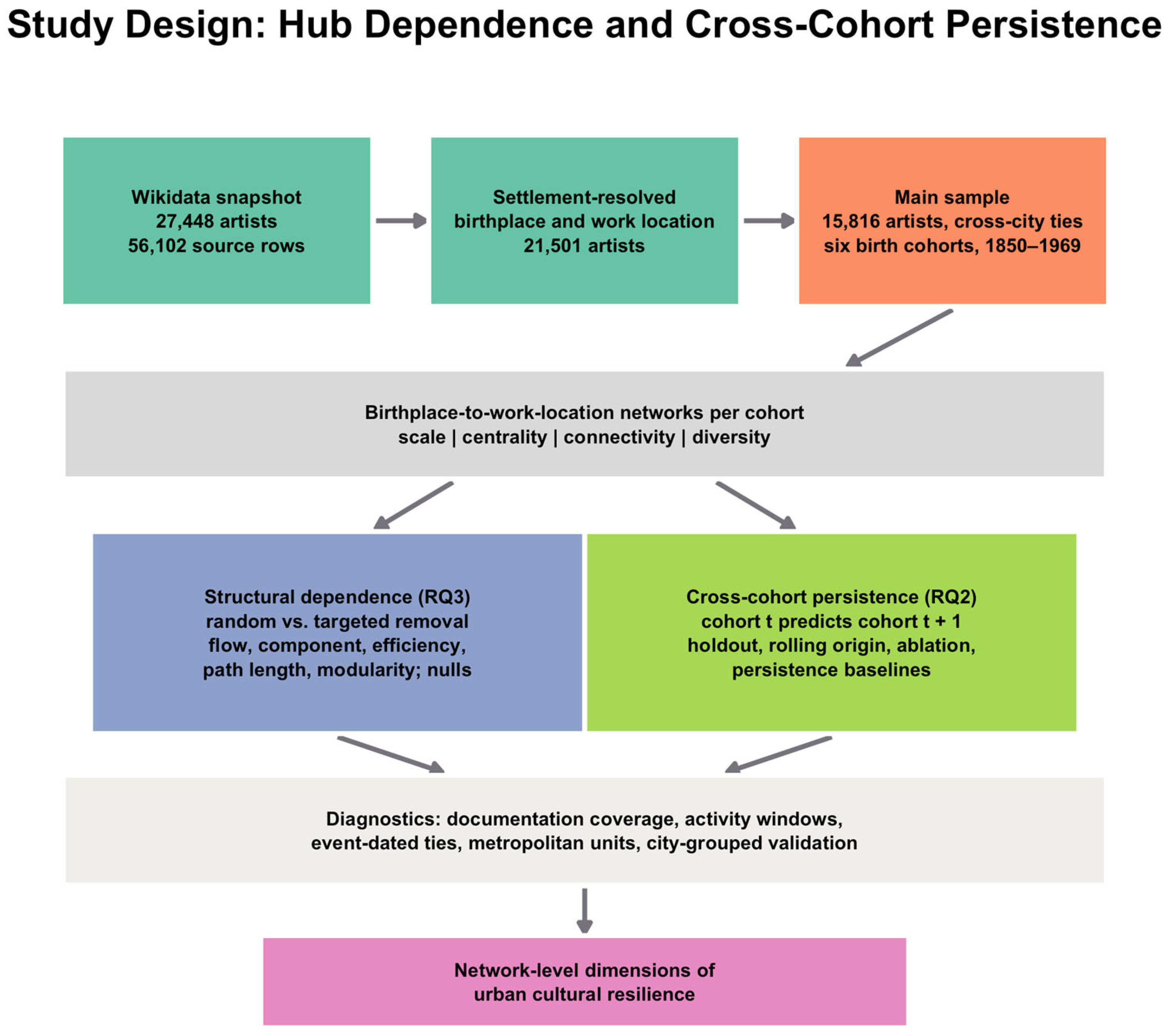
Edges in this study link birthplaces to documented work locations, whereas Schich et al. linked birth to death locations [18]; the destination thus lies in professional life, and an artist can contribute several destinations. Each artist’s contribution is fractionally weighted so that richly documented biographies do not dominate the network. Structural dependence is assessed with several stress-test metrics and benchmarked against degree-preserving null networks. Prospective information is assessed with forward temporal holdouts, rolling-origin folds, persistence baselines, city-grouped validation, and documentation diagnostics. These four features distinguish the design from earlier macro-historical work. The stress tests and the forecasts measure two network-level properties that can be conceptualized as components of urban cultural resilience: structural dependence on hubs and cross-cohort persistence of cultural attraction. Recovery after actual historical shocks, institutional adaptation, and cultural participation lie outside the design. Figure 1 summarizes the study.

Figure 1. Study design. Boxes report the principal sample-size transitions, the two analytical branches (structural dependence and cross-cohort persistence), and the diagnostics added to assess documentation, timing, spatial units, and repeated cities. Box colors mark the stages of the workflow: teal, data retrieval and settlement resolution; orange, the analytical sample; grey, network construction and diagnostics; blue, the structural-dependence branch (RQ3); green, the cross-cohort persistence branch (RQ2); and pink, the network-level dimensions of urban cultural resilience.

2. Materials and Methods

2.1. Data Source and Study Population

Wikidata provides the sampling frame [44]. Data were retrieved in September 2026 and cached locally to preserve the analyzed snapshot of a continuously updated knowledge base. The query identifies human individuals with one of four exact visual-art occupations (painter, sculptor, printmaker, or photographer) and requires a recorded birth date, birthplace (P19), and work location (P937). Restricting the population to these occupations keeps it within visual art and avoids mixing artists with writers, musicians, actors, and architects, whose mobility is governed by different institutions.

The original extraction produced 56,102 artist–work-location rows representing 27,448 unique artists and 11,468 distinct place identifiers. After requiring both birthplace and work location to resolve to settlements (Section 2.2), 21,501 artists remain. The main analysis restricts the sample to artists born from 1850 through 1969 who have at least one cross-city birthplace-to-work-location tie, yielding 15,830 artist–cohort records in six non-overlapping 20-year birth cohorts. These correspond to 15,816 unique artists: 14 artists carry two conflicting birth dates in Wikidata that fall into different cohorts, and they are retained in both cohort networks. Additional attributes were retrieved in October 2026 for the same artist identifiers without redrawing the sample: the number of Wikipedia language editions linked to each item (sitelinks), the numbers of statements and external identifiers, the death date (P570), the work-period start and end (P2031, P2032), the date qualifiers attached to each P937 statement (start time P580, end time P582, point in time P585), the references attached to each P937 statement, and the continent (P30) of each country.

Getty Union List of Artist Names identifiers (Wikidata P245) are retained when available [45]. ULAN linkage serves entity identification: it confirms that a Wikidata item corresponds to an artist recorded in a curated authority file and reduces the risk of conflating homonyms. Population representativeness is a separate matter. Both Wikidata and ULAN reflect the collecting priorities, languages, and institutions that produced them, so ULAN-linked artists share many of the geographic emphases of the full sample. The ULAN-linked rerun reported below therefore tests sensitivity to entity quality, while documentation and coverage bias are examined with the separate diagnostics in Section 2.10.

Wikidata coverage of people varies by language, region, gender, and notability [46,47,48], and a recent audit of humans in Wikidata finds that Western Europe and North America account for most citizenship statements while rural birthplaces are strongly underrepresented [49]. Uneven documentation can therefore shape network structure directly: cities and national art worlds documented by large authority files or active editor communities can appear more central than their historical weight would warrant. The sample is accordingly treated as a large historical sample of documented visual artists. Its country and continent composition is reported in Section 3.1, and the documentation diagnostics in Section 2.10 test how far the main results depend on it.

2.2. Spatial Units and Standardization

Places enter the analysis as the Wikidata items recorded in P19 and P937. An item is retained when it is an instance of human settlement (Q486972) or of any of its subclasses, which covers cities, towns, villages, and municipalities. No population threshold separates cities from smaller settlements, so “city” denotes any settlement node. Items are not merged in the main analysis: separate Wikidata items for a city and for one of its boroughs remain separate nodes, and a place whose name or boundaries changed during the period is represented by its single current Wikidata item and present label. Country attribution uses each item’s current country (P17), so artists born in historical states such as Austria-Hungary or the Russian Empire are assigned to present-day countries. The main analysis therefore uses contemporary geographic entities.

Because historical metropolitan areas often span several present-day items, the main results were re-estimated after harmonizing settlements into metropolitan units. Settlements were ranked by how often they appear in the data; moving down this ranking, each unassigned settlement absorbed all unassigned settlements whose Wikidata coordinates lie within 25 km (and, in a second variant, 50 km). Coordinates are available for 6600 of the 6614 places in the cleaned sample. At 25 km, 3913 places were absorbed into 2701 metropolitan units; at 50 km, 4897 places were absorbed into 1717 units.

2.3. Birthplace-to-Work-Location Ties and Fractional Weighting

The primary relation is a directed tie from an artist’s birthplace to a documented work location:

i: B(i) → W(i,j)

where B(i) is the birthplace of artist i and W(i,j) is the j-th distinct work location recorded for that artist. The tie records that the artist’s documented professional geography includes W(i,j); it carries no information on when the artist arrived there or whether other places came first. An artist may have several work locations. To prevent richly documented biographies from contributing more weight simply because they contain more place statements, each artist’s outgoing contribution is fractionalized. If artist i has k(i) distinct work locations, each tie receives

w(i,j) = 1/k(i)

so the total weight contributed by one artist is one. Same-city birthplace–work-location ties are retained in the artist-level data for documentation but excluded from the inter-city network.

2.4. Birth Cohorts and Approximate Activity Windows

The main specification uses six birth cohorts: 1850–1869, 1870–1889, 1890–1909, 1910–1929, 1930–1949, and 1950–1969. Birth year indexes the generation whose professional geography is observed; it does not date individual moves. Because careers last several decades, the activity periods of adjacent cohorts overlap. To make the temporal reference of each cohort explicit, an approximate activity window was constructed for every artist, running from age 20 to the earlier of death or age 70; the reported work-period start and end dates (P2031, P2032) replace these defaults when available. Each artist contributes equal mass to each year of the window, and the resulting cohort distributions of active years are summarized by their percentiles. Overlap between adjacent cohorts is measured by the overlap coefficient, the sum over calendar years of the smaller of the two normalized distributions; a value of 0 means disjoint activity periods, and 1 means identical ones. A narrower window from age 25 to the earlier of death or age 60 serves as a sensitivity check. Dated P937 statements provide an independent check on the timing implied by the cohorts. In addition, every cross-city tie whose work-location statement carries a date was assigned to the 20-year calendar period of its earliest date, and the concentration, structural dependence, and prediction were re-estimated on the resulting event-dated subnetwork.

2.5. City-Level Measures and Feature Families

For each cohort, cities are nodes and aggregated fractional artist ties are directed weighted edges. City-level measures are grouped into four families that correspond to distinct properties of a city’s position. Scale captures the volume of attraction: weighted in-strength (the sum of incoming fractional weights) and the number of incoming artists. Centrality captures recursive importance within the whole network: PageRank computed on the weighted directed graph with damping 0.85 [50], which rises when a city receives ties from cities that are themselves central. Connectivity captures the number and direction of a city’s distinct links: in-degree (distinct origin cities), out-degree (distinct destination cities of artists born there), and out-strength (the weighted volume of artists born in the city who worked elsewhere). Diversity captures the composition of incoming ties: Shannon entropy of incoming weight across source cities and across source countries, and the number of source countries. Scale and centrality are correlated, yet they answer different questions: scale counts how much a city receives, whereas PageRank also depends on where its ties come from. PageRank therefore forms its own family so that the ablation in Section 2.9 separates the scale from network position. For city c, source diversity is

H(c) = −Σ_j p(c,j) ln p(c,j)

where p(c,j) is the share of city c’s incoming fractional weight originating from source j. Network-level concentration is summarized by the shares of incoming weight captured by the largest one and five destinations and by the Herfindahl index of incoming weight. Table 2 lists the variables and their families.

Table 2. Variables, operational definitions, feature families, and analytical roles.

Variable	Operational Definition	Family/Scale	Analytical Role
Artist tie	Birthplace → documented work location	Directed link between settlement nodes	Biographical spatial association
Fractional weight	1/number of distinct work locations of the artist	Each artist contributes total weight 1	Controls documentation density of biographies
In-strength	Sum of incoming fractional weights	Scale	Current cultural attraction
Incoming artists	Number of distinct incoming artists	Scale	Current cultural attraction
PageRank	Weighted directed PageRank, damping 0.85	Centrality	Recursive network position
In-degree	Number of distinct origin cities	Connectivity	Breadth of recruitment channels
Out-degree	Number of distinct destinations of artists born in the city	Connectivity	Breadth of outward circulation
Out-strength	Sum of outgoing fractional weights	Connectivity	Volume of outward circulation
Source-city entropy	Shannon entropy of incoming weight by origin city	Diversity	Evenness of origin cities
Source-country entropy	Shannon entropy of incoming weight by origin country	Diversity	International evenness of origins
Source countries	Number of distinct origin countries	Diversity	International reach
Future attraction	ln(1 + in-strength in cohort t + 1)	Regression target	Cross-cohort persistence (absolute)
Future attraction share	ln(1 + 1000 × share of cohort t + 1 inflow)	Regression target	Cross-cohort persistence (cohort-normalized)
Future hub	Top quartile of positive in-strength in cohort t + 1	Binary target	Persistent hub status (relative by construction)
Flow retention	Remaining edge weight/intact edge weight	0–1	Structural dependence
Largest component, efficiency, path length, modularity	See Section 2.6	Network level	Structural dependence

2.6. Structural Stress Tests

Random and targeted node removal are compared, following the distinction between random failure and targeted attack in complex-network robustness research [29]. Random failure removes 5%, 10%, 15%, or 20% of cities selected at random, with 30 Monte Carlo replications per cohort and removal fraction. Targeted removal deletes the same proportions of cities in descending order of PageRank computed once on the intact network. Two alternative orderings, by in-strength and by total degree, test whether the results depend on the choice of PageRank [30]. For removal fraction q, the primary outcome is the retained artist-flow weight,

R_F(q) = F(q)/F(0)

where F(0) is the total edge weight before removal and F(q) the weight remaining among surviving cities. Four further metrics describe the residual network: the share of original nodes in the largest weakly connected component; global efficiency, E = [n(n − 1)]⁻¹ Σ_i≠j 1/d_ij, computed on the undirected, unweighted residual network with n surviving nodes and expressed relative to the intact network [31]; the average shortest-path length within the largest connected component; and the modularity of a Louvain partition of the weighted, undirected residual network [51,52], computed with a fixed random seed.

Alongside the proportional removals, the most central city of each cohort was removed on its own, and in a separate scenario, all cities located in one of the three countries receiving the largest inflow were removed together. The country scenario approximates a geographically clustered disruption and is compared with the random removal of an equal number of cities.

A removed node stands for the complete loss of a city’s capacity to receive and send documented artists within a cohort, and the artists who would have gone there are not reassigned to other destinations. Wars, economic crises, and policy shocks rarely work this way; they usually reduce a city’s attraction partially, hit several cities at once, and send artists elsewhere. As topological stress tests, the simulations measure the immediate exposure of the network when no rerouting occurs, an upper bound on damage, and they rank cities by how much network function passes through them. PageRank ordering finds the cities whose loss removes the most function, while the country scenario comes closer to the spatial clustering of many historical disruptions.

2.7. Degree-Preserving Null Networks

Targeted vulnerability could arise mechanically from a skewed degree sequence. Directed null networks were therefore generated via degree-preserving edge swaps [53], with five times as many swaps as edges, and the empirical multiset of edge weights was randomly reassigned to the rewired edges. Thirty null realizations were produced for each cohort. The rewiring preserves the node set, every node’s in-degree and out-degree, the number of edges, and the distribution of edge weights. It alters which cities are connected to which, the assignment of weights to particular ties and hence node strengths, reciprocity, clustering, and the geographic distance spanned by ties. PageRank was recomputed within each null network before targeted removal, so the comparison holds the removal rule constant.

For each cohort and removal fraction, the standardized difference is

z = (R_obs − μ_null)/σ_null

where R_obs is observed flow retention after targeted removal and μ_null and σ_null are the mean and standard deviation of retention across the null realizations. Negative values indicate that the observed network retains less flow than degree-matched random networks, that is, greater structural dependence on its central cities. The empirical percentile of R_obs within the null distribution is reported alongside z.

2.8. Prospective Prediction Design

In the prospective analysis, which is kept separate from the stress tests, features measured in cohort t predict outcomes in cohort t + 1. The primary regression outcome is

Y(c,t + 1) = ln [1 + InStrength(c,t + 1)]

Because the number of documented artists and the total network flow differ across cohorts, an absolute outcome partly reflects the cohort size. Two cohort-normalized outcomes address this: the share of the next cohort’s total inflow received by city c, entered as ln(1 + 1000 × share), and the percentile rank of the city’s next-cohort in-strength among cities in the same transition. A version of the models in which the scale predictors are also expressed as within-cohort shares was estimated as well. The classification outcome identifies whether city c falls in the top quartile of positive incoming flow in cohort t + 1; because the threshold is set within each outcome cohort, this target is relative by construction. Top-10% and top-20% thresholds serve as sensitivity checks.

The predictive sample retains city-cohort observations with at least two incoming artists in cohort t. The main holdout trains on the four earlier transitions and evaluates predictors measured in 1930–1949 against outcomes in 1950–1969, giving 972 training and 315 held-out observations. A rolling-origin analysis repeats the forward-time logic based on three successive held-out transitions; in every fold, the test cohort follows all training cohorts. “Future” therefore denotes the next birth cohort within the 1850–1969 snapshot. The exercise is historical forecasting within a fixed dataset, and the fitted models make no claim to transfer to cohorts born after 1969, whose documented careers are still strongly right-censored.

Elastic Net provides a regularized linear baseline [54]; Random Forest [55] and histogram gradient boosting capture nonlinear relationships; logistic regression and Random Forest are used for hub classification. The main results use hyperparameters fixed in advance (Random Forest: 500 trees, minimum leaf size 3; Elastic Net: α = 0.01, l1 ratio 0.5; gradient boosting: learning rate 0.05, 350 iterations, 31 leaf nodes; logistic regression: C = 1, balanced class weights). To document the effect of tuning, each model was also tuned through nested forward-chaining validation inside the training cohorts: the inner folds trained on 1850–1869 and validated on 1870–1889, trained on 1850–1889 and validated on 1890–1909, and trained on 1850–1909 and validated on 1910–1929. The grids covered the minimum leaf size {1, 3, 5, 10}, maximum features {all, 0.5, √p}, and maximum depth {none, 8} for Random Forest; α {0.001, 0.01, 0.05, 0.1, 0.5} and l1 ratio {0.1, 0.5, 0.9} for Elastic Net; learning rate {0.03, 0.05, 0.1}, leaf nodes {15, 31}, iterations {150, 350}, and minimum leaf size {10, 20} for gradient boosting; and C {0.01, 0.1, 1, 10} for logistic regression. The configuration with the best mean inner-fold R² or ROC-AUC was refitted on all training cohorts and evaluated once on the held-out transition. Classification performance is reported as ROC-AUC, PR-AUC, F1, precision, recall, balanced accuracy, and the confusion matrix at a probability threshold of 0.5.

2.9. Incremental Information, Persistence Baselines, and Repeated Cities

The predictive value is decomposed via feature ablation with eight sets: scale only; scale plus centrality; scale plus connectivity; scale plus diversity; the three pairwise combinations of the network families added to scale; and the full model. Uncertainty in the increment over scale only is quantified with a paired bootstrap of the 315 held-out observations (2000 resamples), recomputing the difference in R² and ROC-AUC between each set and scale only based on identical resamples.

Because the same cities appear in successive cohorts, a model could learn persistent city characteristics instead of the information contained in a given cohort’s network. The simplest check is a linear persistence baseline that predicts the outcome from the logarithm of current in-strength alone. City-history features (the mean and maximum of ln(1 + in-strength) over all earlier cohorts and the number of earlier cohorts in which the city appears) are added to the scale-only and full models to test whether network features add information beyond a city’s accumulated prominence, and city-grouped temporal validation splits the cities of each held-out transition into five groups; for each group, the models are trained on earlier transitions after removing every observation of the held-out cities, so that no city contributes to both training and testing. Performance is also reported separately for held-out cities that never appear in the training panel.

Random-Forest predictions are interpreted with SHAP values computed with the tree explainer [56] for the full regression model fitted to the 972 training observations. The values reported in the main text refer to the 315 held-out observations of the final transition; values for the training observations are reported for comparison. Mean absolute SHAP values are also summed within feature families. They describe how strongly each feature contributes to fitted predictions and carry no causal interpretation.

2.10. Documentation Coverage Diagnostics

Predictors and outcomes are derived from the same Wikidata statements, and documentation is unlikely to be stable across cohorts. Coverage is therefore described cohort by cohort through the median numbers of sitelinks and statements per artist, the share of artists with ULAN identifiers, the mean number of work locations, the shares of P937 statements carrying a date or a reference, and the share of artists with a recorded death date. The predictive models are re-estimated with documentation-intensity controls, namely the weighted means of ln(1 + sitelinks) and ln(1 + statements) among a city’s incoming artists, the weighted ULAN share of those artists, and the mean documentation level of the outcome cohort. They are also re-estimated based on progressively better-documented subsets of artists (at least two, three, and five sitelinks), which serve to repeat the 1950–1969 stress test as well. Concentration measures are recomputed on 300 random subsamples of 2067 artists per cohort, the size of the smallest cohort, for painters alone, and, after excluding artists born in the Netherlands, the most heavily represented country of birth.

2.11. Robustness Analyses

Robustness checks include a rerun based on ULAN-linked artists, alternative future-hub thresholds (top 10%, 20%, and 25%), an alternative 30-year cohort specification, a comparison with degree-preserving null networks, rolling-origin validation, reruns for painters only and excluding photographers, label-permutation tests with 200 randomized outcomes, and geographic-dominance tests that exclude artists born in the Netherlands and, jointly, in the Netherlands, Germany, and the Czech Republic. Further diagnostics cover the event-dated subnetwork, cohort-normalized outcomes, persistence baselines, city-history features, city-grouped validation, hyperparameter tuning, alternative removal orderings, additional stress-test metrics, stylized removal scenarios, and metropolitan harmonization.

2.12. Generative AI Assistance

OpenAI ChatGPT (GPT-5.6 Sol, web interface; accessed in September 2026) was used to assist with writing and debugging the data-analysis code and with English translation and language editing. The research design, interpretation of results, and conclusions were determined by the author. The author checked all code, statistical outputs, numerical values, and references and takes full responsibility for the content of the article. No AI-generated data were added to the research data.

3. Results

3.1. Sample Composition, Documentation, and Activity Windows

Artists born in Europe account for 85.1% of the 15,816 unique artists (Table 3) and those born in North America for 10.0%; Asia, South America, Africa, and Oceania together account for 4.9%. Ten countries account for 81.2% of artists, led by the Netherlands (24.2%), Germany (19.0%), the Czech Republic (12.1%), and the United States (9.0%). France is the birth country of only 2.5% of artists, although Paris is the leading destination of the early cohorts. Destinations are similarly concentrated: 85.6% of artist-flow weight goes to European work locations and 12.1% to North American ones. These proportions describe the documentation of Wikidata at least as much as the historical population of visual artists, and they recur in the diagnostics below.

Table 3. Birth-continent and leading birth-country composition of the main sample by cohort (share of artists).

Birth Region	1850–1869	1870–1889	1890–1909	1910–1929	1930–1949	1950–1969	All
Europe	0.893	0.914	0.901	0.852	0.766	0.816	0.851
North America	0.088	0.062	0.067	0.100	0.163	0.104	0.100
Asia	0.009	0.014	0.019	0.028	0.043	0.039	0.027
South America	0.004	0.006	0.008	0.009	0.015	0.015	0.010
Africa	0.002	0.001	0.002	0.008	0.011	0.018	0.008
Oceania	0.004	0.002	0.003	0.002	0.003	0.008	0.004
Netherlands	0.181	0.247	0.215	0.213	0.240	0.319	0.242
Germany	0.240	0.227	0.185	0.150	0.156	0.184	0.190
United States	0.079	0.057	0.062	0.091	0.150	0.086	0.090
France	0.050	0.038	0.025	0.024	0.011	0.013	0.025

Countries are present-day countries (Wikidata P17) and continents are taken from Wikidata P30; countries spanning two continents are assigned to Europe. Shares are computed over unique artists. The Czech Republic (12.1% of all artists) is the third largest birth country; the full country distribution is given in Table S10. Rows in italics give the leading birth countries.

The median number of Wikipedia language editions per artist falls from 2 in the cohorts born before 1890 to 1 thereafter and the mean from 4.6 to 2.2; the median number of statements falls from 37 to 25.5, the mean number of work locations from 1.79 to 1.35, and the ULAN-linked share from 48% to 32%. Documentation intensity thus declines across cohorts, and later cohorts contain more artists with thin records (Table 4). Between 28% and 45% of P937 statements carry a date, and 87–92% cite at least one reference.

Table 4. Documentation coverage and approximate activity windows by birth cohort.

Cohort	Unique Artists	Sitelinks, Median (Mean)	Statements, Median	ULAN Share	Work Locations, Mean	Dated P937 Share	Active Years, 25th–75th Percentile (Median)	Overlap with Next Cohort	Dated P937 Statements, Median Year (Median Age)
1850–1869	2216	2 (4.6)	37	0.48	1.79	0.43	1890–1915 (1902)	0.58	1890 (30)
1870–1889	2700	2 (4.2)	34	0.39	1.87	0.45	1910–1935 (1922)	0.58	1909 (29)
1890–1909	2354	1 (3.9)	34	0.36	1.74	0.35	1930–1955 (1942)	0.56	1927 (29)
1910–1929	2061	1 (3.9)	33.5	0.35	1.61	0.28	1951–1977 (1964)	0.58	1950 (29)
1930–1949	3129	1 (3.2)	30	0.37	1.43	0.29	1972–1997 (1985)	0.64	1974 (33)
1950–1969	3356	1 (2.2)	25.5	0.32	1.35	0.42	1990–2013 (2001)	–	1992 (32)

Sitelinks = number of Wikipedia language editions linked to the artist’s Wikidata item. Dated P937 share = share of work-location statements with a start time, end time, or point in time. Active years run from age 20 to the earlier of death or age 70 (reported work periods replace these defaults when available); overlap is the overlap coefficient of the active-year distributions of adjacent cohorts (0 = disjoint, 1 = identical). Fourteen artists have conflicting birth dates in Wikidata that place them in two cohorts; they are counted once here and in both cohort networks elsewhere.

The middle half of the approximate active years of the 1850–1869 cohort falls between 1890 and 1915, that of the 1910–1929 cohort between 1951 and 1977, and that of the 1950–1969 cohort between 1990 and 2013 (Table 4; Figure S7). Adjacent cohorts share 56–64% of their activity distributions under the main window and 45–51% under the narrower window. The dated work-location statements agree with this mapping: their median year rises from 1890 for the 1850–1869 cohort to 1992 for the 1950–1969 cohort, the median age at the dated statement lies between 29 and 33, and 95–99% of dated statements fall between ages 15 and 75. Each cohort network therefore describes the professional geography of a generation whose activity is centered 41–45 years after the midpoint of its birth years and overlaps substantially with that of the next generation. The prospective design thus predicts a city’s attraction for a generation that becomes active about twenty years after the predictor generation, while a large part of both generations’ activity falls in the same decades.

The 7631 cross-city ties whose work location carries a date (32.7% of all cross-city ties; 5350 artists) were assigned to 20-year calendar periods by their earliest date. City in-strength in each dated period correlates with in-strength in the birth cohort whose median activity falls in that period (Pearson r between 0.66 and 0.76 on the logarithmic scale), and 55–70% of the twenty leading destinations coincide (Table S9), which supports the temporal reading of the cohorts. The dated subcorpus is heavily Dutch (38–64% of artists born in the Netherlands), so it tests the temporal mapping of the cohorts and leaves the question of representativeness open.

3.2. Cohort Networks and Concentration

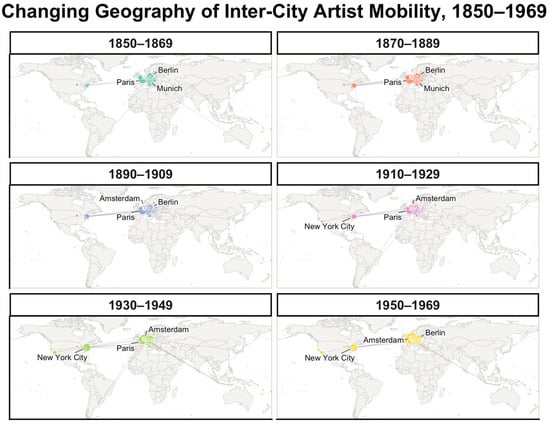
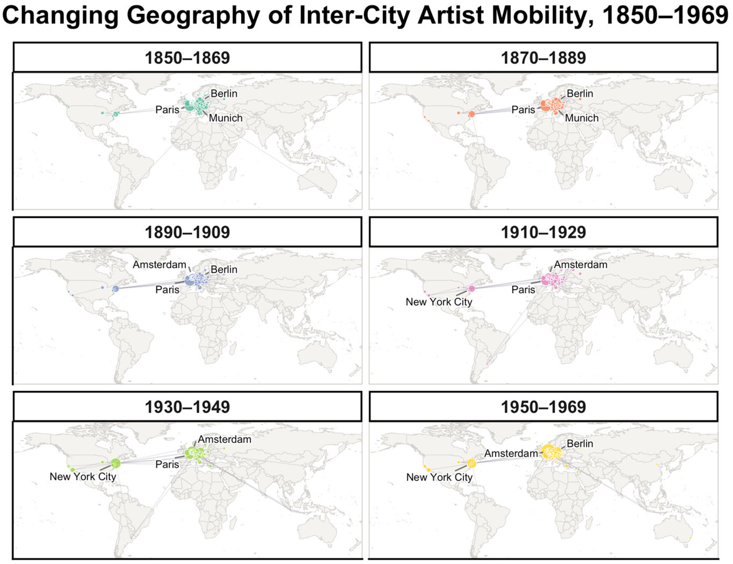
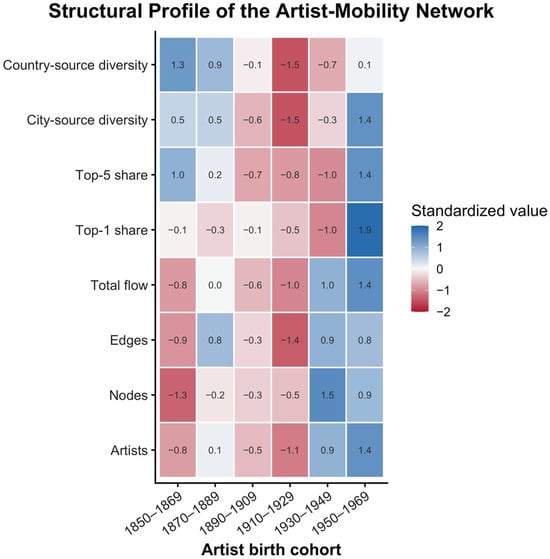
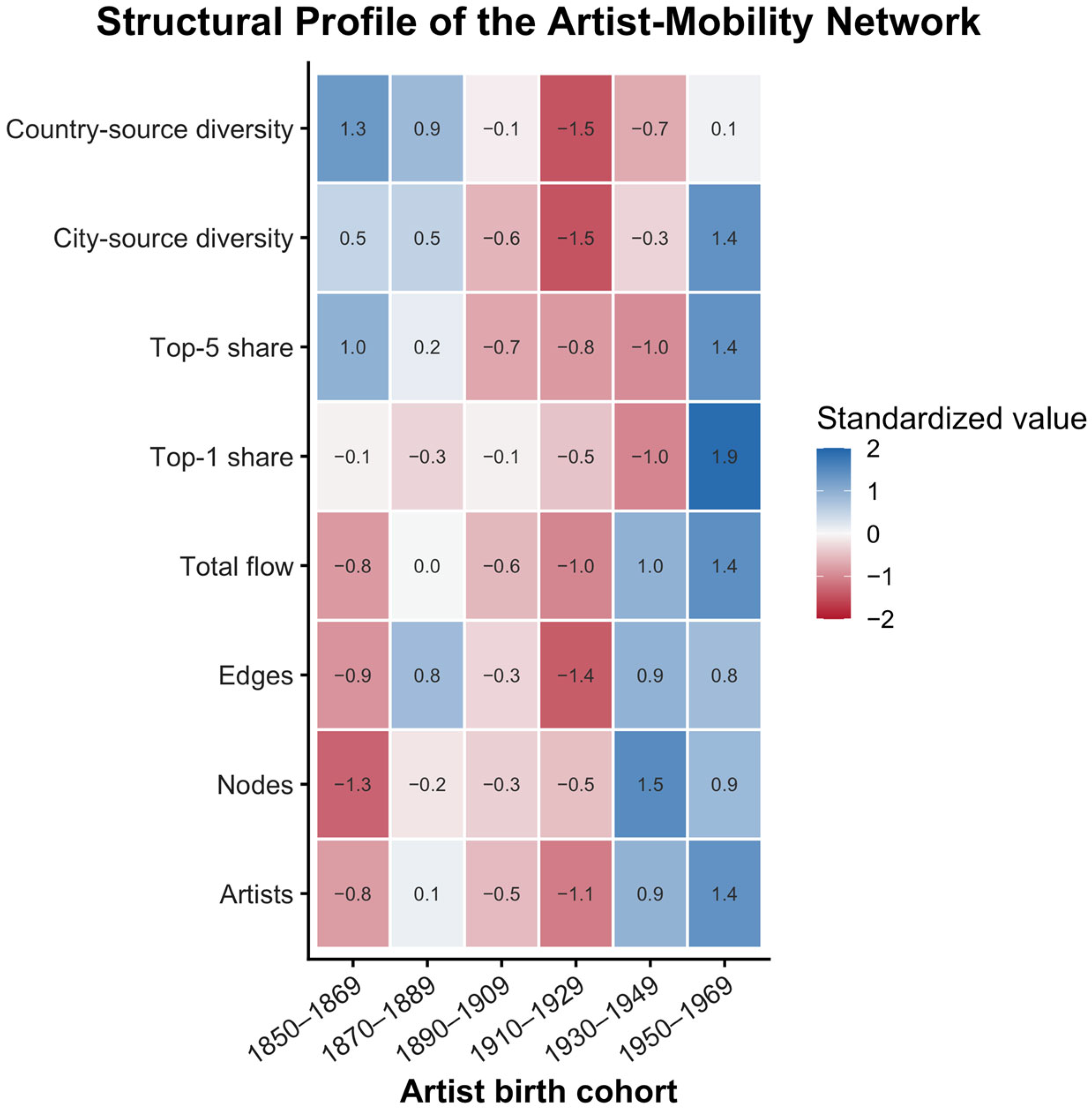
The six cohort networks contain between 1503 and 2162 city nodes and between 2621 and 3552 directed edges (Table 5). Paris is the largest destination for the four cohorts born between 1850 and 1929 and Amsterdam for the two cohorts born between 1930 and 1969; Munich, Berlin, Vienna, London, and New York are the other recurrent leading destinations. The largest destination receives about 10% of incoming weight in the first three cohorts, 9.1% in 1910–1929, 7.7% in 1930–1949, and 14.8% in 1950–1969, while the five largest destinations together receive between one quarter and one third. Figure 2 shows the geographic backbone of each cohort network, and Figure 3 places network size, total flow, concentration, and source diversity on a common standardized scale.

Table 5. Descriptive statistics and concentration of the six birth-cohort networks.

Cohort	Artists	Nodes	Edges	Total Fractional Flow	Largest Destination	Top-1 Share	Top-5 Share	Top-1 share, Size-Equalized (95% Interval)	Top-1 Share, Excl. Netherlands-Born
1850–1869	2216	1503	2818	2061.4	Paris	0.101	0.323	0.101 (0.097–0.104)	0.116 (Paris)
1870–1889	2702	1775	3501	2515.2	Paris	0.095	0.293	0.095 (0.089–0.100)	0.112 (Paris)
1890–1909	2357	1731	3049	2206.8	Paris	0.101	0.260	0.101 (0.097–0.105)	0.116 (Paris)
1910–1929	2067	1694	2621	1964.6	Paris	0.091	0.256	0.091 (–)	0.102 (Paris)
1930–1949	3129	2162	3552	3023.3	Amsterdam	0.077	0.252	0.077 (0.072–0.083)	0.087 (New York)
1950–1969	3359	2017	3495	3273.4	Amsterdam	0.148	0.339	0.148 (0.139–0.157)	0.079 (Berlin)
Total	15,830	–	–	15,044.7	–	–	–	–	–

Artists are counted once, in their birth cohort; the six cohort counts sum to 15,830. Nodes and edges are cohort-specific and are not summed. The total fractional flow is smaller than the number of artists because work locations in the birthplace itself carry weight but form no inter-city tie. Size-equalized shares are means over 300 random subsamples of 2067 artists (the size of the smallest cohort, which therefore has no sampling interval).

Figure 2. Geography of birthplace-to-work-location ties across the six 20-year birth cohorts. Each panel displays the 140 highest-weight inter-city edges and 70 leading destination nodes; the node size represents incoming fractional artist weight and the three largest destinations are labeled.

Figure 3. Standardized structural profile of the six cohort networks. Rows combine the network scale, total flow, hub concentration, and weighted source-diversity measures. Values are z-scores standardized within each metric across cohorts and clipped to the displayed range.

When every cohort is reduced to 2067 randomly drawn artists, the top-1 share of 1950–1969 remains 0.148 (95% interval 0.139–0.157), well above the 0.072–0.105 range of the earlier cohorts (Table 5), so the cohort size does not account for the rise. The share of photographers rises from 23.5% of artists in 1850–1869 to 39.5% in 1950–1969, while the share of painters falls from 70.3% to 53.2%; among painters alone, the top-1 share of 1950–1969 (0.124) is close to that of the cohorts born before 1910 (0.116–0.122). Artists born in the Netherlands make up between 18% and 25% of the earlier cohorts and 31.9% of the 1950–1969 cohort, and most of the inflow to Amsterdam in that cohort comes from them. Excluding Netherlands-born artists lowers the 1950–1969 top-1 share to 0.079, with Berlin as the largest destination, and turns the series into a steady decline, from 0.116 for Paris in 1850–1869 to 0.087 for New York in 1930–1949 and 0.079 for Berlin in 1950–1969 (Table 5). The high concentration of the latest cohort therefore reflects the weight of a densely documented Dutch subcorpus, and, among artists born elsewhere, the network becomes steadily less centered on a single destination.

3.3. Structural Dependence on Hubs

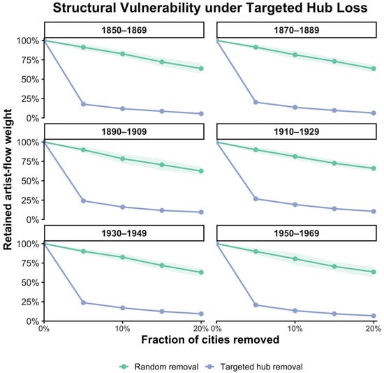
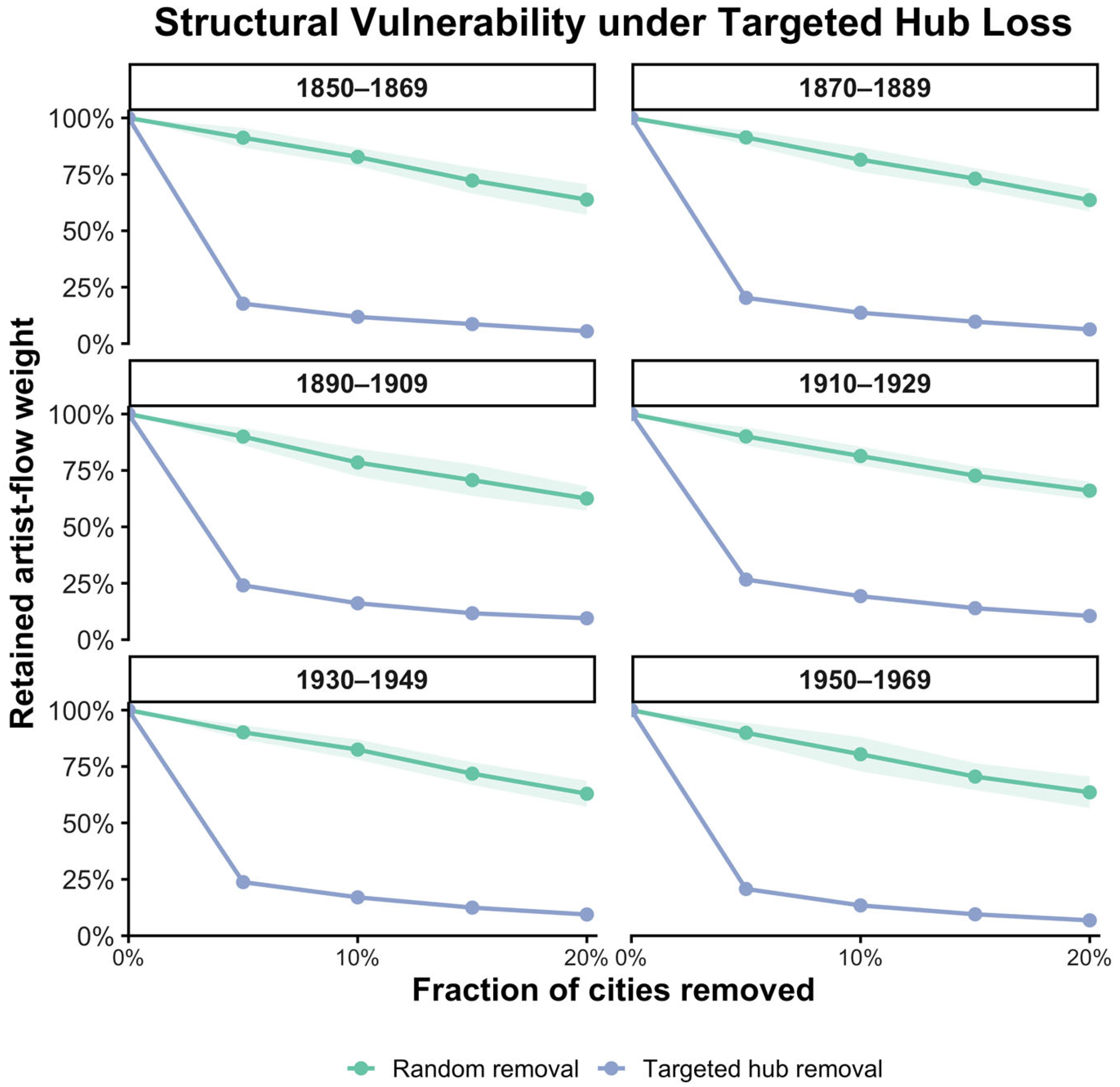
In the 1950–1969 network, removing the 5% of cities with the highest PageRank leaves 20.7% of artist-flow weight and removing 10% leaves 13.4%, whereas random removal of the same proportions leaves 90.0% and 80.4% on average. Across the six cohorts, targeted removal of 5% of cities leaves between 17.7% and 26.6% of flow, against about 90% under random removal (Figure 4).

Figure 4. Retained artist-flow weight under random and targeted node removal across the six cohorts. Targeted removal follows descending PageRank computed on the intact network; random removal is averaged over 30 Monte Carlo replications, and the shaded band shows one standard deviation.

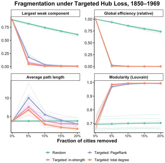
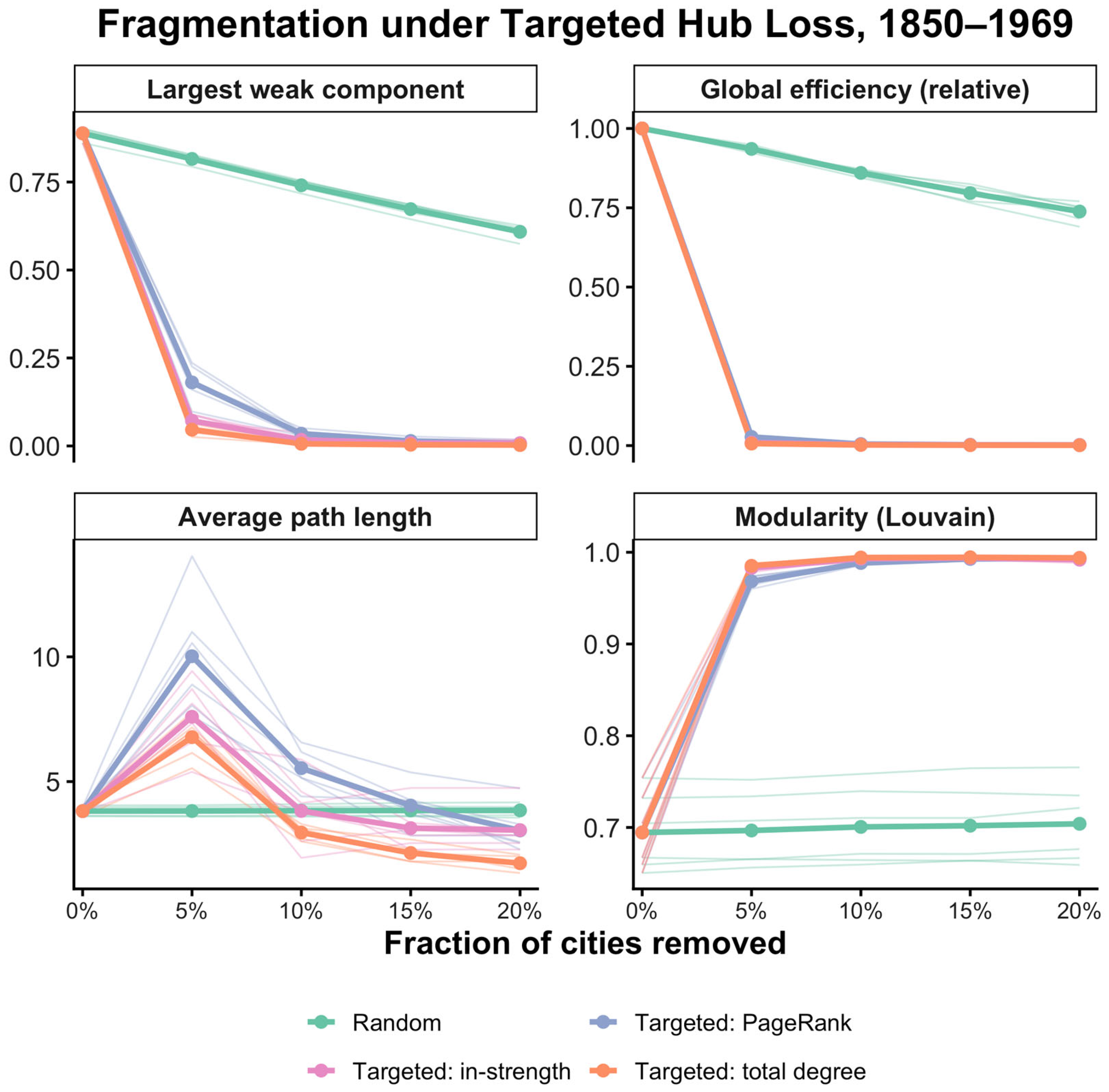
In 1950–1969, removing the top 5% of cities by PageRank shrinks the largest weakly connected component from 89.6% to 22.6% of nodes, against 82.2% under random removal; global efficiency falls to 3.3% of its intact value, against 93.1%; the average path length within the largest component rises from 3.8 to 10.6 steps as the remaining component is held together by long chains; and modularity rises from 0.66 to 0.96 as the residual network splits into nearly disconnected clusters, while random removal leaves modularity unchanged (0.67) (Figure S6). The same sequence recurs in every cohort (Figure 5). Path length peaks at 5% removal and then falls again, because the largest component has by then shrunk to a small cluster, so targeted removal fragments the network, in addition to draining its flow. Ordering removal by in-strength or by total degree is at least as damaging as ordering by PageRank: in 1950–1969, these orderings leave 16.5% and 16.9% of flow at 5% removal and 10.0% and 10.6% at 10% removal. The result is therefore robust to the choice of targeting rule.

Figure 5. Fragmentation under targeted hub loss across the six birth cohorts. Thin lines show individual cohorts and thick lines their mean, for random removal (30 replications per cohort) and three targeted orderings: share of original nodes in the largest weakly connected component, global efficiency relative to the intact network, average shortest-path length within the largest connected component, and Louvain modularity of the residual network. The 1950–1969 cohort is shown in detail in Figure S6.

At 5% targeted removal, observed retention lies between 2.5 and 4.5 standard deviations below the null mean and, at 10% removal, between 2.2 and 5.7 standard deviations below (Table 6). In eleven of the twelve comparisons, the observed value lies below every null realization, so all six observed networks depend more on their central cities than degree-preserving randomized networks do. Because the null networks keep every city’s in-degree and out-degree, the excess dependence comes from where ties and weights are placed: heavy ties converge on the same few destinations more strongly than the degree sequence alone would produce.

Table 6. Observed flow retention after targeted PageRank removal compared with directed degree-preserving null networks (30 realizations per cohort).

Cohort	Removed	Observed Retention	Null Mean	Null SD	z	Empirical Percentile
1850–1869	5%	0.177	0.215	0.009	−4.07	0.00
1850–1869	10%	0.118	0.147	0.008	−3.70	0.00
1870–1889	5%	0.203	0.233	0.012	−2.53	0.00
1870–1889	10%	0.137	0.153	0.007	−2.20	0.03
1890–1909	5%	0.241	0.280	0.009	−4.53	0.00
1890–1909	10%	0.161	0.200	0.007	−5.72	0.00
1910–1929	5%	0.266	0.313	0.012	−3.87	0.00
1910–1929	10%	0.193	0.218	0.009	−2.87	0.00
1930–1949	5%	0.238	0.276	0.011	−3.64	0.00
1930–1949	10%	0.170	0.200	0.007	−4.32	0.00
1950–1969	5%	0.207	0.252	0.011	−4.08	0.00
1950–1969	10%	0.134	0.177	0.009	−4.57	0.00

z = (observed − null mean)/null SD; negative values indicate lower retention, i.e., greater dependence on central cities, than in degree-preserving randomized networks. The empirical percentile is the share of null realizations with retention at or below the observed value.

Removing only the single most central city (Paris for the cohorts born 1850–1929, Amsterdam for 1930–1969) removes between 9.3% and 16.7% of all artist-flow weight, whereas removing one random city removes about 0.1%. Removing every city in a country has more varied effects. Removing all German settlements, which make up 17–23% of nodes, leaves 66–80% of flow, comparable to or higher than the random removal of the same number of cities, because German ties are spread over many small places. Removing all Dutch settlements from the 1950–1969 network (17.7% of nodes) leaves 60.2% of flow, against 69.2% for an equally large random removal (Table S8). The flow structure around hubs is summarized in Table 7. Ties from non-hub origins to the 5% most central cities carry 46–53% of all artist-flow weight in each cohort, ties among hubs 19–25%, ties from hubs to non-hub cities 5–9%, and lateral ties between non-hub cities 18–27%. Only 20–29% of lateral flow crosses a national border. Between 69% and 78% of non-hub origin cities send most of their outgoing artist weight to hubs, and between 50% and 61% send all of it.

Table 7. Composition of artist-flow weight by link type relative to the 5% most central cities (PageRank), by cohort.

Cohort	Hubs (n)	Non-Hub → Hub	Hub → Hub	Hub → Non-Hub	Non-Hub → Non-Hub	Cross-Border Share of Non-Hub → Non-Hub	Non-Hub Origins Sending Most Outflow to Hubs	Non-Hub Origins Sending all Outflow to Hubs
1850–1869	75	0.534	0.239	0.049	0.177	0.262	0.780	0.612
1870–1889	89	0.486	0.251	0.061	0.203	0.282	0.738	0.539
1890–1909	87	0.476	0.195	0.088	0.241	0.268	0.707	0.502
1910–1929	85	0.467	0.189	0.078	0.266	0.288	0.691	0.505
1930–1949	108	0.460	0.215	0.088	0.238	0.227	0.691	0.523
1950–1969	101	0.490	0.249	0.054	0.207	0.198	0.730	0.571

Shares of total fractional artist-flow weight in each cohort; the four link types sum to one. Hubs are the 5% of cities with the highest PageRank in the cohort network.

3.4. Prospective Prediction of Next-Cohort Attraction

Prospective performance is evaluated on cities observed in 1930–1949, with outcomes measured in 1950–1969 (Table 8). With the hyperparameters fixed before the analysis, Random Forest predicts log next-cohort in-strength with R² = 0.750 (RMSE = 0.583; MAE = 0.479), Elastic Net with R² = 0.733, and gradient boosting with R² = 0.707. Nested forward-chaining tuning changes these values little: the tuned Random Forest (minimum leaf size 5, √p features per split, maximum depth 8) reaches R² = 0.758, the tuned Elastic Net 0.734, and the tuned gradient boosting 0.743. For future top-quartile hub status, logistic regression reaches ROC-AUC = 0.867 and Random Forest 0.866, with PR-AUC = 0.891 for both. At a probability threshold of 0.5, Random Forest identifies 128 of the 162 future hubs (recall 0.790) with 29 false positives (precision 0.815), and logistic regression identifies 122 (recall 0.753) with 25 false positives (precision 0.830). Tuning raises the Random-Forest ROC-AUC to 0.871. The two classifier families perform almost identically, so the evidence concerns the stability of the predictive signal across model families; no family is clearly superior.

Table 8. Prospective model performance based on the final temporal holdout (predictors 1930–1949, outcomes 1950–1969; training n = 972, test n = 315).

Model (Task, Hyperparameters)	R2	RMSE	MAE	ROC-AUC	PR-AUC	F1	Precision	Recall	TN/FP/FN/TP
Elastic Net (regression, fixed)	0.733	0.603	0.494	–	–	–	–	–	–
Elastic Net (regression, tuned)	0.734	0.602	0.493	–	–	–	–	–	–
Random Forest (regression, fixed)	0.750	0.583	0.479	–	–	–	–	–	–
Random Forest (regression, tuned)	0.758	0.575	0.474	–	–	–	–	–	–
Hist. gradient boosting (regression, fixed)	0.707	0.632	0.512	–	–	–	–	–	–
Hist. gradient boosting (regression, tuned)	0.743	0.592	0.490	–	–	–	–	–	–
Logistic regression (classification, fixed)	–	–	–	0.867	0.891	0.790	0.830	0.753	128/25/40/122
Logistic regression (classification, tuned)	–	–	–	0.868	0.892	0.788	0.834	0.747	129/24/41/121
Random Forest (classification, fixed)	–	–	–	0.866	0.891	0.803	0.815	0.790	124/29/34/128
Random Forest (classification, tuned)	–	–	–	0.871	0.894	0.806	0.845	0.772	130/23/37/125

Regression metrics refer to ln(1 + next-cohort in-strength). Classification metrics refer to top-quartile hub status in 1950–1969 (162 of 315 held-out cities are positive); threshold-dependent metrics and the confusion matrix (true negatives/false positives/false negatives/true positives) use a probability threshold of 0.5. Tuned models were selected by nested forward-chaining validation within the training cohorts (Section 2.8).

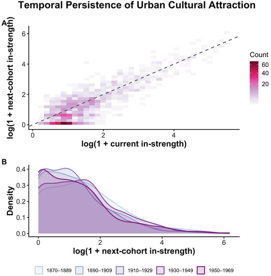
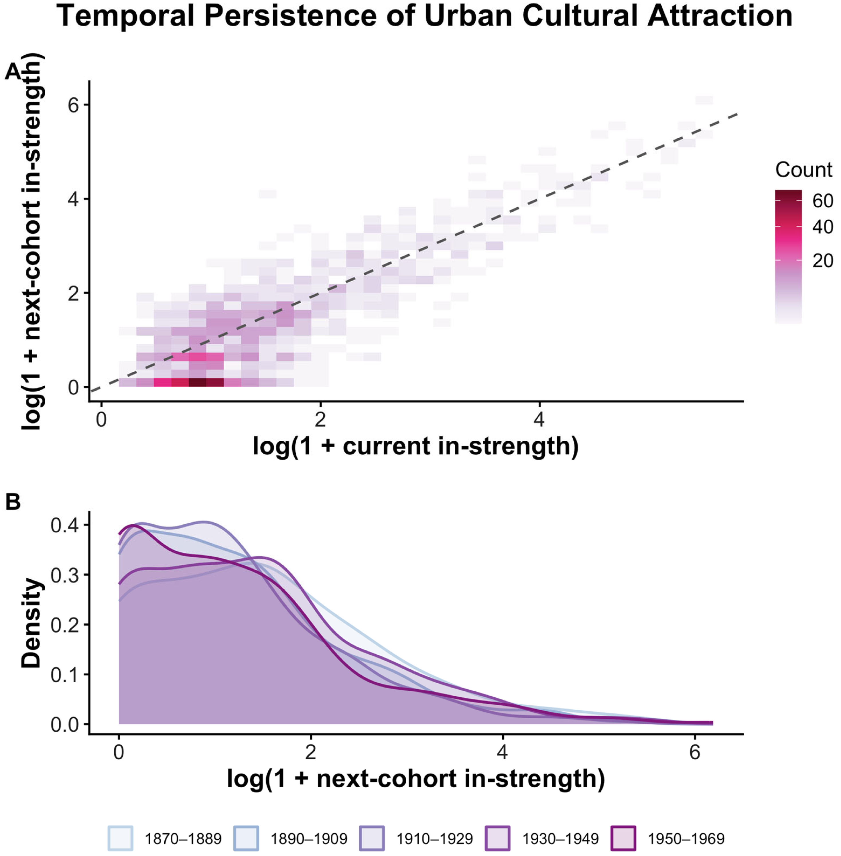
Across the full panel, current and next-cohort in-strength are strongly aligned, and the distribution of next-cohort attraction keeps a long right tail in every outcome cohort (Figure 6).

Figure 6. Temporal persistence of urban cultural attraction. Panel (A) is a two-dimensional histogram of current versus next-cohort in-strength across the prospective panel; Panel (B) shows the density of next-cohort attraction by outcome cohort.

3.5. Network Information Beyond Current Scale

Once PageRank is moved out of the baseline, current scale alone explains 73.3% of held-out variance in next-cohort attraction and reaches ROC-AUC = 0.827 for future hub status (Table 9). Adding PageRank to the scale does not improve either task. Adding connectivity raises the R² to 0.749 and ROC-AUC to 0.849, and the full model reaches R² = 0.750 and ROC-AUC = 0.866. The paired bootstrap places the regression increment of the full model at ΔR² = 0.017 (95% interval −0.011 to 0.047) and the classification increment at ΔAUC = 0.039 (0.012 to 0.067). The network structure therefore adds a modest amount of information for the continuous outcome, an amount that cannot be distinguished from zero in this holdout, and a clearer amount for identifying which cities will be among the leading destinations. Connectivity carries most of this gain; centrality and diversity add little on their own. Logistic regression shows the same ordering for classification (ROC-AUC 0.848 with scale only, 0.867 with all features).

Table 9. Feature-set ablation on the final temporal holdout (Random Forest), with paired-bootstrap intervals for the increment over scale only.

Feature Set	R2	ΔR2 vs. Scale (95% Interval)	ROC-AUC	ΔAUC vs. Scale (95% Interval)	PR-AUC	F1
Scale	0.733	–	0.827	–	0.845	0.734
Scale + centrality	0.711	−0.022 (−0.053 to 0.006)	0.827	0.000 (−0.025 to 0.027)	0.864	0.725
Scale + connectivity	0.749	0.016 (−0.009 to 0.044)	0.849	0.022 (−0.005 to 0.051)	0.876	0.765
Scale + diversity	0.725	−0.008 (−0.027 to 0.010)	0.821	−0.006 (−0.026 to 0.017)	0.849	0.751
Scale + centrality + connectivity	0.747	0.014 (−0.015 to 0.045)	0.860	0.033 (0.006 to 0.062)	0.882	0.783
Scale + centrality + diversity	0.724	−0.009 (−0.037 to 0.017)	0.837	0.010 (−0.015 to 0.036)	0.867	0.749
Scale + connectivity + diversity	0.746	0.013 (−0.014 to 0.042)	0.852	0.025 (0.001 to 0.052)	0.878	0.779
Full	0.750	0.017 (−0.011 to 0.047)	0.866	0.039 (0.012 to 0.067)	0.891	0.803

Scale = in-strength and incoming artists; centrality = PageRank; connectivity = in-degree, out-degree, and out-strength; diversity = source-city entropy, source-country entropy, and number of source countries. Intervals are 2.5th and 97.5th percentiles of 2000 paired bootstrap resamples of the 315 held-out cities.

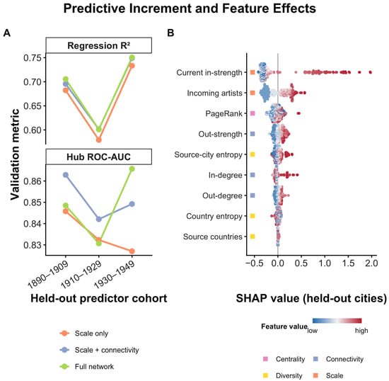
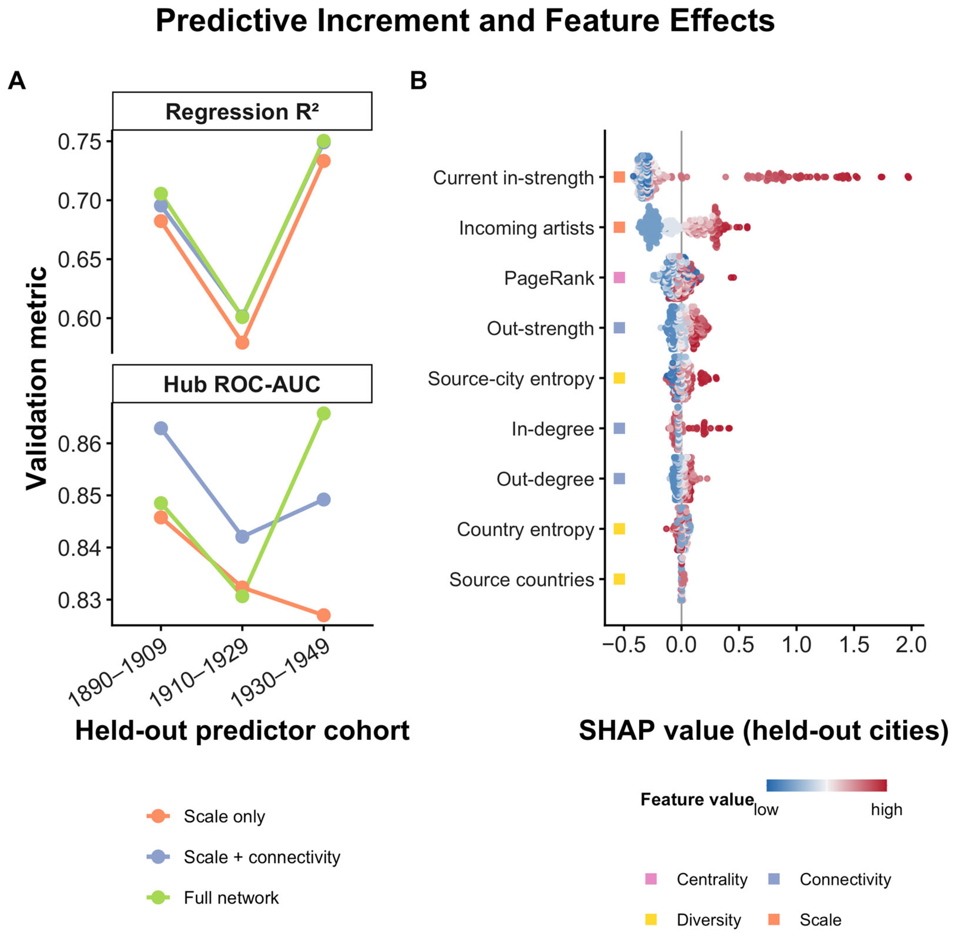
Across the three rolling-origin holdouts (Figure 7A), the mean R² is 0.665 for scale only, 0.682 with connectivity, and 0.686 for the full model; the full model improves on scale only in all three folds, by 0.017–0.023. The mean ROC-AUC is 0.835 for scale only, 0.851 with connectivity, and 0.848 for the full model; adding connectivity improves classification in all three folds, by 0.010–0.022, whereas the full model’s gain varies between −0.002 and 0.039.

Figure 7. Predictive increment and feature effects. Panel (A)compares scale-only, scale-plus-connectivity, and full-network Random-Forest models across the three rolling-origin holdouts for the regression R² and hub-classification ROC-AUC. Panel (B) shows the SHAP value of every feature for each of the 315 held-out cities of the final transition (full regression model), with features ordered by mean absolute SHAP value; the point color gives the feature’s percentile within the held-out sample, and squares mark the feature family.

A linear model using only the logarithm of current in-strength reaches R² = 0.709 and ROC-AUC = 0.842 on the final holdout, close to the Random-Forest scale model. Adding each city’s history of prominence in all earlier cohorts changes the regression performance little (R² = 0.739 for the full model with history, against 0.750 without) and raises the ROC-AUC slightly to 0.879 (Table 10). Under city-grouped temporal validation, where no city contributes to both training and testing, the full model still outperforms the scale-only model on the final holdout (R² = 0.749 vs. 0.725; ROC-AUC = 0.865 vs. 0.826) and in the 1910–1929 fold (R² = 0.605 vs. 0.568). Prediction is weak for the 53–92 held-out cities that never appear in the training panel (R² between −0.27 and 0.25; ROC-AUC between 0.61 and 0.78), and network features do not improve it. The persistence of individual cities therefore accounts for much of what the models learn, and the network increment concerns the way established cities are connected.

Table 10. Persistence baselines, city-history features, and city-grouped validation (Random Forest unless stated).

Held-Out Predictor Cohort	Specification	R2	ROC-AUC
1890–1909	Linear persistence baseline (ln current in-strength)	0.706	0.833
1890–1909	Scale	0.682	0.846
1890–1909	Full network	0.706	0.849
1890–1909	Full network + city history	0.718	0.861
1890–1909	City-grouped: scale/full	0.688/0.708	0.850/0.844
1910–1929	Linear persistence baseline	0.585	0.835
1910–1929	Scale	0.579	0.832
1910–1929	Full network	0.601	0.831
1910–1929	Full network + city history	0.601	0.846
1910–1929	City-grouped: scale/full	0.568/0.605	0.834/0.840
1930–1949	Linear persistence baseline	0.709	0.842
1930–1949	Scale	0.733	0.827
1930–1949	Full network	0.750	0.866
1930–1949	Full network + city history	0.739	0.879
1930–1949	City-grouped: scale/full	0.725/0.749	0.826/0.865

City history = mean and maximum of ln(1 + in-strength) over all earlier cohorts and the number of earlier cohorts in which the city appears. City-grouped validation removes all observations of the held-out cities from the training cohorts (five city groups per holdout).

SHAP values computed on the held-out observations attribute 68% of mean absolute contribution to the scale family, 17% to connectivity, 8% to centrality, and 7% to diversity; the training observations give almost the same shares (68%, 17%, 8%, and 8%). Current in-strength and incoming artists dominate, followed by PageRank, out-strength, source-city entropy, in-degree, and out-degree (Figure 7B). The beeswarm also shows the direction of these effects: high values of in-strength, incoming artists, out-strength, and in-degree raise predicted attraction, and a handful of cities with very large current inflow account for the long right tail of the in-strength contributions.

3.6. Robustness

When the outcome is a city’s share of next-cohort inflow, the full Random-Forest model reaches R² = 0.776 against 0.774 for scale only; with scale predictors also expressed as within-cohort shares, the values are 0.808 and 0.778. When the outcome is the within-transition percentile rank, the full model reaches R² = 0.604 against 0.550. Across the rolling-origin folds, mean R² for the share outcome is 0.738 for the full model and 0.729 for scale only. The prediction of relative attraction is thus as accurate as the prediction of absolute attraction, and the network increment remains small (Table 11).

Table 11. Robustness of the prospective results and of structural dependence (Random Forest; final holdout unless stated).

Specification	Test n	R2 Scale	R2 Full	ROC-AUC Scale	ROC-AUC Full	Targeted 5% Retention, 1950–1969
Main specification	315	0.733	0.750	0.827	0.866	0.207
Outcome: share of next-cohort inflow	315	0.774	0.776	–	–	–
Share outcome, cohort-normalized predictors	315	0.778	0.808	–	–	–
Outcome: within-transition percentile rank	315	0.550	0.604	–	–	–
Documentation-intensity controls added	315	0.748	0.755	0.843	0.875	–
Artists with ≥ 2 sitelinks	163	0.690	0.705	0.821	0.848	0.273
Artists with ≥ 3 sitelinks	112	0.669	0.714	0.780	0.839	0.304
Artists with ≥ 5 sitelinks	72	0.701	0.754	0.820	0.862	0.354
City-grouped temporal validation	315	0.725	0.749	0.826	0.865	–
Metropolitan harmonization, 25 km	248	0.717	0.741	0.867	0.881	0.187
Metropolitan harmonization, 50 km	200	0.735	0.739	0.899	0.917	0.172
Event-dated network (1970–1989 → 1990–2009)	75	0.706	0.731	0.888	0.926	0.115–0.257 *
ULAN-linked artists	127	–	0.702	–	0.896	–
Painters only	224	–	0.691	–	0.857	–
Excluding photographers	255	–	0.689	–	0.834	–
Excluding Netherlands-born artists	262	–	0.688	–	0.821	–
Excluding artists born in the Netherlands, Germany, and the Czech Republic	177	–	0.654	–	0.825	–
30-year cohorts, outcome 1970–1989	–	–	−0.304	–	–	–

Scale = in-strength and incoming artists; full = all nine network features. * Range across the seven dated calendar periods; random removal of 5% leaves 0.89–0.92. Rows with a dash under “scale” report specifications estimated for the full model only.

Adding the documentation intensity of each city’s incoming artists raises the scale-only performance to R² = 0.748 and ROC-AUC = 0.843, and the full model with the same controls reaches 0.755 and 0.875; adding the documentation level of the outcome cohort changes little (0.747 and 0.878), so the classification increment survives documentation controls. Based on subsets restricted to better-documented artists (at least two, three, or five Wikipedia language editions; 7556, 4910, and 2923 artists), the full model outperforms the scale-only model in every case (R² 0.705–0.754 against 0.669–0.701; ROC-AUC 0.839–0.862 against 0.780–0.821). The targeted removal of 5% of cities in 1950–1969 leaves 27–35% of flow in these subsets, against 20.7% in the full sample: hub dependence is somewhat weaker among better-documented artists, which is consistent with thinly documented artists contributing a single recorded work location in a major center. The event-dated subnetwork reproduces both main results. Targeted removal of 5% of cities leaves 11.5–25.7% of flow in each calendar period against 89–92% under random removal, and in the one transition with enough dated ties for a holdout (predictors 1970–1989, outcomes 1990–2009; 75 test cities), the full model outperforms scale only (R² = 0.731 against 0.706; ROC-AUC = 0.926 against 0.888).

The ULAN-linked subset reproduces the main temporal pattern (R² = 0.702; ROC-AUC = 0.896). Hub classification is stable across thresholds (ROC-AUC 0.903, 0.881, and 0.866 for the top 10%, 20%, and 25%). Painters only (R² = 0.691; ROC-AUC = 0.857) and the sample excluding photographers (0.689; 0.834) give slightly lower but similar results. The observed final-period R² and ROC-AUC exceed all 200 label-permutation replications (permutation p = 0.005). Metropolitan harmonization within 25 km reduces the number of nodes by about half and leaves the conclusions intact: in 1950–1969, the targeted removal of 5% of metropolitan units leaves 18.7% of flow against 90.7% under random removal, and the full model reaches R² = 0.741 and ROC-AUC = 0.881 against 0.717 and 0.867 for scale only; the 50 km variant gives similar values. The 30-year specification that uses the 1970–1989 cohort as the outcome period fails out of sample (R² = −0.30), consistent with the right-censoring of younger artists’ documented careers.

Excluding artists born in the Netherlands lowers the R² to 0.688 and ROC-AUC to 0.821; excluding artists born in the Netherlands, Germany, and the Czech Republic lowers them to 0.654 and 0.825, with the held-out sample falling from 315 to 177 cities. The signal survives these exclusions, yet it is not independent of the geographic concentration of the source data and of the countries that dominate it.

4. Discussion

4.1. Prominence and Structural Dependence

Current inflow predicts next-cohort inflow well; a single logarithmic term already reaches R² = 0.71 in the final holdout. In the same networks, removing the most central 5% of cities removes about four-fifths of artist-flow weight, breaks the largest component apart, and lowers global efficiency to a few percent of its intact level, and degree-preserving randomized networks with the same degree sequence retain more flow in every cohort. The cities that remain attractive across generations are thus the cities through which most of the network’s ties run, and prominence and structural dependence describe two sides of the same concentration.

Early cohorts are oriented toward Paris, Munich, Berlin, Vienna, and London, and New York and Amsterdam gain prominence later, which matches the durable but shifting centers described by Schich et al. [18] and the clustering of important visual artists documented with art-dictionary data [11,12]. The present results extend that literature from where artists concentrate to how the network feeding those concentrations depends on them. Between 69% and 78% of non-hub origin cities send most of their outgoing artists to the 5% most central cities, and lateral ties between non-hub cities carry less than a quarter of all flow in most cohorts.

Because the simulations let the artists of a removed city simply leave the network, they give an upper bound on damage. Losing Paris or Amsterdam alone costs 9–17% of a cohort’s flow, whereas removing every German settlement costs no more than an equally large random removal because German ties are spread over many small places. Dependence is therefore concentrated in particular cities more than in national systems. How far actual disruptions, such as the German occupation of Paris in 1940 or the emigration of artists from Central Europe in the 1930s, redirected artists to other destinations is a question that the topology alone cannot answer.

4.2. How Much Network Structure Adds

For the continuous outcome, the full model improves on scale only by 0.017 in R² on the final holdout and by 0.017–0.023 in each rolling fold, and the bootstrap interval for the final holdout includes zero. For future hub status, the gain is larger and more stable: the ROC-AUC rises by 0.039 (95% interval 0.012–0.067) on the final holdout, connectivity improves classification in all three rolling folds, and the gain survives documentation controls and city-grouped validation. Logistic regression and Random Forest perform almost identically, which indicates a predictive signal that is stable across model families. In practice, ranking cities by current inflow recovers most of the information contained in the full model. Connectivity adds value at the margin of the hub category, where cities of a similar size differ in how many places they draw artists from and send artists to.

SHAP attributes 17% of mean absolute contribution to connectivity and 7% to diversity, the ablation shows that connectivity carries the gain while diversity and centrality add little once scale is known, and correlations among predictors are reported in Figure S3; connectivity and diversity are thus partly distinct from scale in this dataset. Counting PageRank with scale lowers the scale baseline to R² = 0.711 and makes the network increment appear larger; with PageRank treated as a network feature, the regression increment shrinks to the values reported here.

Prediction is weak for cities entering the panel for the first time, city-history features leave the network increment in place, and city-grouped validation retains it. The network component of the forecast therefore concerns how established cities are connected, and anticipating the emergence of new centers remains beyond the reach of these features.

4.3. Possible Mechanisms Linking Connectivity to Later Attraction

Cumulative advantage accounts for the dominance of scale: cities that already attract artists accumulate institutions, markets, teachers, and reputations that draw later cohorts [13,57,58]. The design identifies associations only, and for the connectivity increment, three channels are plausible. In-degree counts the distinct origin cities from which a city recruits; a city fed by many origins depends less on the continued output of any single pipeline, and its recruitment rests on many weak ties [59]. Out-degree and out-strength measure how many artists born in a city work elsewhere; cities embedded in two-way circulation keep alumni, correspondents, and dealers in other centers, and these contacts can channel later arrivals, as in chain migration and in the transnational careers documented for artist communities [10,22]. PageRank records the second-order position, the extent to which a city receives artists from places that are themselves central, which parallels the effect of early access to central institutions on artistic careers [23,24]. Source diversity can matter through the recombination of styles and training traditions [60,61], although its predictive contribution here is small. Testing these mechanisms requires event-dated careers, institutional data, and research designs built around historical shocks.

4.4. Documentation and the Meaning of Concentration

The rise in the top-city share in 1950–1969 follows the growth of the Dutch subcorpus and disappears when Netherlands-born artists are excluded, leaving a steady decline in the top-city share from 0.116 to 0.079 across the six cohorts. Documentation intensity falls across cohorts, and structural dependence is weaker among better-documented artists. ULAN linkage improves entity identification without changing these patterns. The core results nevertheless survive every diagnostic: hub dependence exceeds the degree-preserving benchmark in all cohorts and appears in metropolitan units, in well-documented subsets, and in event-dated networks, and the network increment for hub classification survives documentation controls and city grouping. The findings describe the documented network of visual artists in Wikidata, a network that is predominantly European and in which Dutch, German, and Czech artists are overrepresented relative to French artists. How closely the historical cultural system matched its documented trace is a question that this source cannot settle.

4.5. Implications for Cultural Policy

Lateral ties between non-hub cities carry 18–27% of flow, and only a fifth to a quarter of them cross national borders; these are the ties that survive the loss of hubs. Residency exchanges, co-commissioning, and touring circuits between second-tier cities in different countries, of the kind organized through city-to-city cooperation such as the UNESCO Creative Cities Network, would thicken this layer. Between 69% and 78% of non-hub origin cities send most of their artists to hubs, and half send all of them; regional academies, studio programs, and exhibition venues in intermediate cities would give artists from these origins alternative first destinations. Flows from hubs to non-hub cities are small (5–9% of weight), so fellowships and teaching posts that bring artists trained in central cities to smaller ones would turn one-directional recruitment into circulation. Lateral cross-border links, alternative first destinations, and return circulation from hubs are thus the clearest targets that the link typology identifies. For monitoring, PageRank-based exposure measures identify the cities whose loss would remove most of the network function and can guide contingency support, such as emergency relocation residencies, when a central city faces a crisis [4,43]. These implications are derived from historical documented networks; contemporary artist mobility operates under different institutions and would need its own data before specific programs are designed.

5. Limitations and Future Research

The ties analyzed here are spatial associations between birthplace and documented work locations. About a third of cross-city ties carry dates, and the dated subnetwork reproduces the main results, yet the sequence, timing, and duration of moves remain unknown for most artists. Birth cohorts also index generations whose activity periods overlap by more than half, so the predictive design forecasts the attraction of a later generation that is partly active at the same time as the predictor generation. Career trajectories reconstructed from exhibition catalogues, academy registers, address books, and the biographical sections of authority files would separate first moves from return migration and repeated circulation and would allow networks and forecasts to be built in calendar time.

City-history features and city-grouped validation show that the network increment is not reducible to persistent city prominence, whereas prediction for cities without an observed history remains weak; panel models with city fixed effects and longer histories could separate the time-varying network position from stable city characteristics more completely. Normalized outcomes remove most of the cohort-size component of the absolute outcome, although cohort sizes themselves reflect documentation.

Coverage is the deeper constraint. Wikidata and ULAN are uneven across countries, languages, periods, occupations, and levels of notability, and the sample is predominantly European with a strong Dutch, German, and Czech presence. Documentation controls, well-documented subsets, and geographic exclusions narrow this bias without eliminating it. The spatial units add a second layer of uncertainty: they are contemporary Wikidata settlements and present-day countries, and although metropolitan harmonization at 25 and 50 km leaves the results unchanged, historical boundaries, renamed places, and changing national affiliations are not modeled. Reweighting artists by estimated documentation propensity, combining several authority files, adding non-Western biographical sources, and linking places to historical gazetteers and period-specific administrative units are priorities for future work.

The node-removal experiments are topological stress tests without rerouting, and the temporal models establish the out-of-period association. Recovery and adaptation can be studied only around actual disruptions, such as wars, occupations, and forced emigration, where the redistribution of artists after the shock is observed, and institutions, art markets, migration regimes, and education systems would need to enter the analysis alongside the network measures before causal claims become possible.

6. Conclusions

This study measures two network-level properties of historical birthplace-to-work-location networks of visual artists that can be conceptualized as components of urban cultural resilience. The first is structural dependence on hubs. In every birth cohort from 1850 to 1969, removing the most central 5% of cities removes about four-fifths of the artist-flow weight and fragments the network, far beyond the effect of random removal or of removal from degree-preserving randomized networks. The second is cross-cohort persistence. A city’s current inflow predicts its inflow in the next cohort, and connectivity adds a small, consistent increment that is clearest for identifying future hubs. Both properties hold under cohort-normalized outcomes, city-grouped validation, metropolitan harmonization, documentation controls, and event-dated networks, while the high concentration of the latest cohort reflects the density of Dutch documentation.

The contribution is a measurable network perspective on cultural persistence and structural vulnerability. It specifies a cultural system, two relational functions, and the conditions under which these functions persist or are exposed. This perspective captures one dimension of urban cultural resilience, to be read alongside institutional, social, economic, and participatory dimensions that require other kinds of data.

References

- Soini, K.; Birkeland, I. Exploring the scientific discourse on cultural sustainability. Geoforum 2014, 51, 213–223. [Google Scholar] [CrossRef] [Scilit]
- Dessein, J.; Soini, K.; Fairclough, G.; Horlings, L. (Eds.) Culture in, for and as Sustainable Development; University of Jyväskylä: Jyväskylä, Finland, 2015. [Google Scholar]
- Soini, K.; Dessein, J. Culture-Sustainability Relation: Towards a Conceptual Framework. Sustainability 2016, 8, 167. [Google Scholar] [CrossRef] [Scilit]
- UNESCO. Global Report on Cultural Policies: Culture—The Missing SDG; UNESCO: Paris, France, 2025. [Google Scholar]
- Holling, C.S. Resilience and Stability of Ecological Systems. Annu. Rev. Ecol. Syst. 1973, 4, 1–23. [Google Scholar] [CrossRef] [Scilit]
- Martin, R.; Sunley, P. On the notion of regional economic resilience: Conceptualization and explanation. J. Econ. Geogr. 2015, 15, 1–42. [Google Scholar] [CrossRef] [Scilit]
- Meerow, S.; Newell, J.P.; Stults, M. Defining urban resilience: A review. Landsc. Urban Plan. 2016, 147, 38–49. [Google Scholar] [CrossRef] [Scilit]
- Markusen, A.; Gadwa, A. Arts and Culture in Urban or Regional Planning: A Review and Research Agenda. J. Plan. Educ. Res. 2010, 29, 379–391. [Google Scholar] [CrossRef] [Scilit]
- Komorowski, M.; Lupu, R.; Pepper, S.; Lewis, J. Joining the Dots—Understanding the Value Generation of Creative Networks for Sustainability in Local Creative Ecosystems. Sustainability 2021, 13, 12352. [Google Scholar] [CrossRef] [Scilit]
- Hautala, J.; Nordström, P. Creative city, mobility, and creativity: Finnish artists in Berlin. Mobilities 2019, 14, 859–874. [Google Scholar] [CrossRef] [Scilit]
- Kelly, E.; O’Hagan, J. Geographic clustering of economic activity: The case of prominent western visual artists. J. Cult. Econ. 2007, 31, 109–128. [Google Scholar] [CrossRef] [Scilit]
- O’Hagan, J.; Hellmanzik, C. Clustering and Migration of Important Visual Artists: Broad Historical Evidence. Hist. Methods 2008, 41, 121–136. [Google Scholar] [CrossRef] [Scilit]
- Hellmanzik, C. Location matters: Estimating cluster premiums for prominent modern artists. Eur. Econ. Rev. 2010, 54, 199–218. [Google Scholar] [CrossRef] [Scilit]
- O’Hagan, J.; Borowiecki, K.J. Birth Location, Migration, and Clustering of Important Composers. Hist. Methods 2010, 43, 81–90. [Google Scholar] [CrossRef] [Scilit]
- Borowiecki, K.J. Agglomeration economies in classical music. Pap. Reg. Sci. 2015, 94, 443–468. [Google Scholar] [CrossRef] [Scilit]
- Serafinelli, M.; Tabellini, G. Creativity over time and space. J. Econ. Growth 2022, 27, 1–43, Correction in J. Econ. Growth 2022, 28, 337–338. [Google Scholar] [CrossRef] [Scilit]
- Borowiecki, K.J.; Graddy, K. Immigrant artists: Enrichment or displacement? J. Econ. Behav. Organ. 2021, 191, 785–797. [Google Scholar] [CrossRef] [Scilit]
- Schich, M.; Song, C.; Ahn, Y.-Y.; Mirsky, A.; Martino, M.; Barabási, A.-L.; Helbing, D. A network framework of cultural history. Science 2014, 345, 558–562. [Google Scholar] [CrossRef] [Scilit]
- Laouenan, M.; Bhargava, P.; Eyméoud, J.-B.; Gergaud, O.; Plique, G.; Wasmer, E. A cross-verified database of notable people, 3500BC–2018AD. Sci. Data 2022, 9, 290. [Google Scholar] [CrossRef] [Scilit]
- Yu, A.Z.; Ronen, S.; Hu, K.; Lu, T.; Hidalgo, C.A. Pantheon 1.0, a manually verified dataset of globally famous biographies. Sci. Data 2016, 3, 150075. [Google Scholar] [CrossRef] [Scilit]
- Joyeux-Prunel, B. Provincializing Paris. The Center-Periphery Narrative of Modern Art in Light of Quantitative and Transnational Approaches. Artl@s Bull. 2015, 4, 4. [Google Scholar]
- Buchholz, L. What is a Global Field? Theorizing Fields beyond the Nation-State. Sociol. Rev. 2016, 64, 31–60. [Google Scholar] [CrossRef] [Scilit]
- Fraiberger, S.P.; Sinatra, R.; Resch, M.; Riedl, C.; Barabási, A.-L. Quantifying reputation and success in art. Science 2018, 362, 825–829. [Google Scholar] [CrossRef] [Scilit]
- de Nooy, W. The dynamics of artistic prestige. Poetics 2002, 30, 147–167. [Google Scholar] [CrossRef] [Scilit]
- Montalto, V.; Tacao Moura, C.J.; Langedijk, S.; Saisana, M. Culture counts: An empirical approach to measure the cultural and creative vitality of European cities. Cities 2019, 89, 167–185. [Google Scholar] [CrossRef] [Scilit]
- Montalto, V.; Alberti, V.; Panella, F.; Sacco, P.L. Are cultural cities always creative? An empirical analysis of culture-led development in 190 European cities. Habitat Int. 2023, 132, 102739. [Google Scholar] [CrossRef] [Scilit]
- Grossi, E.; Sacco, P.L.; Tavano Blessi, G. Cultural, creative, and complex: A computational foundation of culture-driven urban governance. Cities 2023, 140, 104437. [Google Scholar] [CrossRef] [Scilit]
- Lee, H.; Jacoby, N.; Hennequin, R.; Moussallam, M. Mechanisms of cultural diversity in urban populations. Nat. Commun. 2025, 16, 5192. [Google Scholar] [CrossRef] [Scilit]
- Albert, R.; Jeong, H.; Barabási, A.-L. Error and attack tolerance of complex networks. Nature 2000, 406, 378–382, Correction in Nature 2001, 409, 542. [Google Scholar] [CrossRef] [Scilit]
- Holme, P.; Kim, B.J.; Yoon, C.N.; Han, S.K. Attack vulnerability of complex networks. Phys. Rev. E 2002, 65, 056109. [Google Scholar] [CrossRef] [Scilit]
- Latora, V.; Marchiori, M. Efficient Behavior of Small-World Networks. Phys. Rev. Lett. 2001, 87, 198701. [Google Scholar] [CrossRef] [Scilit]
- Pendall, R.; Foster, K.A.; Cowell, M. Resilience and regions: Building understanding of the metaphor. Camb. J. Reg. Econ. Soc. 2010, 3, 71–84. [Google Scholar] [CrossRef] [Scilit]
- Schippers, H. Cities as Cultural Ecosystems: Researching and Understanding Music Sustainability in Urban Settings. J. Urban Cult. Res. 2016, 12, 10–19. [Google Scholar] [CrossRef]
- Dovey, J.; Moreton, S.; Sparke, S.; Sharpe, B. The practice of cultural ecology: Network connectivity in the creative economy. Cult. Trends 2016, 25, 87–103. [Google Scholar] [CrossRef] [Scilit]
- de Bernard, M.; Comunian, R.; Gross, J. Cultural and creative ecosystems: A review of theories and methods, towards a new research agenda. Cult. Trends 2022, 31, 332–353. [Google Scholar] [CrossRef] [Scilit]
- Ratiu, D.E. Creative cities and/or sustainable cities: Discourses and practices. City Cult. Soc. 2013, 4, 125–135. [Google Scholar] [CrossRef] [Scilit]
- Kirchberg, V.; Kagan, S. The roles of artists in the emergence of creative sustainable cities: Theoretical clues and empirical illustrations. City Cult. Soc. 2013, 4, 137–152. [Google Scholar] [CrossRef] [Scilit]
- Montalto, V.; Sacco, P.L.; Saisana, M. Cultural, Creative, and Sustainable Cities: Assessing Progress and Measurement Perspectives. Sustainability 2022, 14, 4246. [Google Scholar] [CrossRef] [Scilit]
- Stefanidou, A.; Doumpos, M.; Zopounidis, C. Culture as a driver of sustainable urban development—Methodological approaches. Dev. Sustain. Econ. Financ. 2024, 2–4, 100011. [Google Scholar] [CrossRef] [Scilit]
- Zhao, Q.; Zhang, L.; Hou, J. Developing a cultural sustainability assessment framework for environmental facilities in urban communities. npj Herit. Sci. 2025, 13, 107. [Google Scholar] [CrossRef] [Scilit]
- Fabbricatti, K.; Boissenin, L.; Citoni, M. Heritage Community Resilience: Towards new approaches for urban resilience and sustainability. City Territ. Archit. 2020, 7, 17. [Google Scholar] [CrossRef] [Scilit]
- Zeng, X.; Ortner, F.P.; Tunçer, B. Systematic Review of the Role of Arts Places in Fostering Urban Sustainability and Resilience. Sustainability 2025, 17, 2076. [Google Scholar] [CrossRef] [Scilit]
- Comunian, R.; England, L. Creative and cultural work without filters: Covid-19 and exposed precarity in the creative economy. Cult. Trends 2020, 29, 112–128. [Google Scholar] [CrossRef] [Scilit]
- Wikidata Contributors. Wikidata. Available online: https://www.wikidata.org/ (accessed on 15 October 2026).
- Getty Trust, J.P.; Getty Research Institute. Union List of Artist Names (ULAN). Available online: https://www.getty.edu/research/tools/vocabularies/ulan/ (accessed on 27 September 2026).
- Färber, M.; Bartscherer, F.; Menne, C.; Rettinger, A. Linked data quality of DBpedia, Freebase, OpenCyc, Wikidata, and YAGO. Semant. Web 2018, 9, 77–129. [Google Scholar] [CrossRef] [Scilit]
- Wagner, C.; Graells-Garrido, E.; Garcia, D.; Menczer, F. Women through the glass ceiling: Gender asymmetries in Wikipedia. EPJ Data Sci. 2016, 5, 5. [Google Scholar] [CrossRef] [Scilit]
- Yu, Y.; Li, X.; Li, T.; Dhillon, P.S.; Romero, D.M. Demographic disparity in Wikipedia coverage: A global perspective. EPJ Data Sci. 2025, 14, 15. [Google Scholar] [CrossRef] [Scilit]
- Kronk, C. Initial Evaluation of Potential Bias in Coverage of Humans in Wikidata. arXiv 2026, arXiv:2609.22375. [Google Scholar]
- Brin, S.; Page, L. The anatomy of a large-scale hypertextual Web search engine. Comput. Netw. ISDN Syst. 1998, 30, 107–117. [Google Scholar] [CrossRef] [Scilit]
- Blondel, V.D.; Guillaume, J.-L.; Lambiotte, R.; Lefebvre, E. Fast unfolding of communities in large networks. J. Stat. Mech. 2008, 2008, P10008. [Google Scholar] [CrossRef] [Scilit]
- Newman, M.E.J. Modularity and community structure in networks. Proc. Natl. Acad. Sci. USA 2006, 103, 8577–8582. [Google Scholar] [CrossRef] [Scilit]
- Maslov, S.; Sneppen, K. Specificity and Stability in Topology of Protein Networks. Science 2002, 296, 910–913. [Google Scholar] [CrossRef] [Scilit]
- Zou, H.; Hastie, T. Regularization and Variable Selection via the Elastic Net. J. R. Stat. Soc. B 2005, 67, 301–320. [Google Scholar] [CrossRef] [Scilit]
- Breiman, L. Random Forests. Mach. Learn. 2001, 45, 5–32. [Google Scholar] [CrossRef] [Scilit]
- Lundberg, S.M.; Lee, S.-I. A Unified Approach to Interpreting Model Predictions. In Advances in Neural Information Processing Systems 30; Curran Associates: Red Hook, NY, USA, 2017. [Google Scholar]
- Merton, R.K. The Matthew Effect in Science. Science 1968, 159, 56–63. [Google Scholar] [CrossRef] [Scilit]
- Barabási, A.-L.; Albert, R. Emergence of Scaling in Random Networks. Science 1999, 286, 509–512. [Google Scholar] [CrossRef] [Scilit]
- Granovetter, M.S. The Strength of Weak Ties. Am. J. Sociol. 1973, 78, 1360–1380. [Google Scholar] [CrossRef] [Scilit]
- Uzzi, B.; Spiro, J. Collaboration and Creativity: The Small World Problem. Am. J. Sociol. 2005, 111, 447–504. [Google Scholar] [CrossRef] [Scilit]
- Burt, R.S. Structural Holes and Good Ideas. Am. J. Sociol. 2004, 110, 349–399. [Google Scholar] [CrossRef] [Scilit]
Disclaimer/Publisher’s Note: The statements, opinions and data contained in all publications are solely those of the individual author(s) and contributor(s) and not of MDPI and/or the editor(s). MDPI and/or the editor(s) disclaim responsibility for any injury to people or property resulting from any ideas, methods, instructions or products referred to in the content. |
© 2026 by the author. Licensee MDPI, Basel, Switzerland. This article is an open access article distributed under the terms and conditions of the Creative Commons Attribution (CC BY) license.