Sustainable Biogas Utilization in Wastewater Treatment Plants: A Predictive-Optimization Decision-Making Framework for CHP Investments and Operations

Abstract

Although biogas and combined heat and power (CHP) technologies are mature, the economic feasibility of energy recovery depends on plant operations, technology costs, and energy prices. This study develops a decision-support framework integrating multilinear regression for biogas prediction, stochastic natural-gas price modeling using a mean-reverting process, and mixed-integer linear programming (MILP) to evaluate digester operation and CHP technology selection under uncertain market conditions. The framework was applied retrospectively to a 55 MGD wastewater treatment plant with thermal hydrolysis pretreatment already installed and substantial biogas flaring. Digester-specific regression models were calibrated using 2022–2023 records and evaluated against prepared 2024 observations, yielding R² values of 0.68–0.78. Four natural-gas price scenarios were evaluated through 100 stochastic runs per scenario. CHP technology selections were more consistent under high and extreme gas-price scenarios and more variable under low and reference scenarios. Reported undiscounted payback periods were >20, 18.9, 16.4, and 12.3 years for the low, reference, high, and extreme scenarios, respectively. Higher natural-gas prices increased modeled avoided energy costs and shortened investment recovery periods. The results support preliminary screening of CHP pathways under alternative gas-price conditions, with economic performance remaining conditional on the modeled operating and cost assumptions.

1. Introduction

By the end of 2025, nearly 2600 biogas systems were operating across all U.S. sectors, including 1232 wastewater systems [1]. The Environmental Protection Agency (EPA) reports that more than half of the wastewater systems use at least some of their biogas for electricity or useful heat [2]. Methane has a 100-year global warming potential approximately 27–30 times greater than that of CO₂ [3]; therefore, capturing methane from organic waste through biogas systems not only reduces greenhouse gas emissions but also converts it into a valuable renewable energy source for heat, electricity, and renewable natural gas, supporting more sustainable waste management.

Anaerobic digestion (AD) stabilizes municipal sewage sludge, reduces volatile solids, and produces methane-rich biogas [4,5]. To improve digestion efficiency and reduce sludge-management costs, pretreatment methods such as mechanical, chemical, enzymatic, and thermal treatment have been explored before mesophilic digestion [6]. Their effectiveness depends on sludge characteristics and operating conditions, while practical application is influenced by trade-offs involving energy use, chemical requirements, downstream effects, and cost [6].

In this context, Barber (2016) [7] highlights that when facilities approach capacity limits, thermal hydrolysis pretreatment (THP) can improve sludge biodegradability and increase the organic loading rates (OLRs) that existing digesters can process in some configurations. THP is a mature pretreatment technology applied before anaerobic digestion. Commercial high-temperature THP uses pressurized heating, often followed by rapid decompression. Lower-temperature thermal pretreatment, including treatment below 100 °C, has also been investigated and can improve subsequent digestion; its performance depends in part on exposure time and sludge characteristics [8]. Growing interest and project development reflect potential energy-recovery and biosolids-management benefits, but higher capital and operating costs are not necessarily offset at every facility [7,8].

For a facility where THP is already installed, the immediate energy decision is how to use the biogas produced under that existing digestion configuration. Biogas systems represent a mature technological pathway for industries seeking environmental benefits and energy security, with combined heat and power (CHP) being a common energy-recovery option for digesters [9]. The International Energy Agency (IEA) task 37 report provides production and consumption patterns in ten countries, offers insights into the role of biogas in decarbonization, as well as production sources, end use, and industrial applications [9]. Major biogas-to-electricity technologies include chemical, electrochemical, thermal-electric, and thermal-mechanical systems. Internal combustion engines are generally the most economical at small scales, while gas turbines are more common for large-scale generation, and Stirling engines remain limited because of their relatively low thermal efficiency [10]. This aligns with the U.S. Department of Energy’s (DOE) CHP technology review [11], which uses the DOE CHP installation database [12] to compare technology deployment. Among the five main prime movers, reciprocating engines and gas turbines account for 55% of installations, and 64% of installed capacity, as of 2018.

Recently, interest in CHP has grown across the energy and environmental sectors [13]. The EPA’s feasibility analysis documentation [14], focused on industrial facilities, provides studies showing how CHP reduces electrical load by reusing waste heat and emphasizes sizing systems to meet thermal demand even when electrical output exceeds on-site needs. The reported results highlight the strong influence of natural gas price variability on marginal generation cost savings. Historical data show that U.S. natural gas prices have experienced substantial fluctuations over the past decade, affecting fuel-cost assumptions and potentially changing CHP payback periods, particularly for facilities with continuous thermal demand such as WWTPs [15]. This sensitivity to fuel-price assumptions supports examining a range of energy-price conditions in CHP feasibility and technology selection analyses, rather than relying solely on static or average price projections.

Although CHP systems can convert on-site biogas into useful electricity and heat and may provide favorable economic returns, their feasibility depends strongly on plant-specific conditions. The case study in [16] reported a payback period of approximately 5.7 years when sufficient biogas production and thermal demand were available. However, project-development requirements, operation and maintenance demands, biogas impurities, and gas-cleaning costs can limit CHP implementation and reduce its economic attractiveness. Historically, CHP deployment was much more limited; as of 2011, only about 3.3% of U.S. WWTPs utilized biogas for electricity production through cogeneration [16].

Existing research relevant to CHP decision-making falls into three streams. First, data-driven studies predict biogas production from feed and operating measurements; Sun et al. (2023) [17], for example, evaluated prediction models using full-scale WWTP data. Second, optimization studies address biogas use and energy operation. Oluleye et al. (2019) [18] selected biogas-use technologies using real WWTP inputs and included capital and operating costs; Laing et al. (2020) [19] optimized gas distribution using historical plant data. Other studies explicitly address uncertainty: Tavakoli et al. (2021) [20] modeled uncertain day-ahead energy prices in a biogas energy hub, and Stuhlmacher et al. (2025) [21] considered uncertain biogas production when scheduling a WWTP generator. Third, techno-economic studies evaluate CHP and THP. Riley et al. (2020) [16] assessed CHP at a WWTP; Elio and Milcarek (2022) [22] showed that hourly rather than annual biogas and demand data changed estimated CHP size and savings; and Balasundaram et al. (2025) [23] compared conventional and THP-assisted digestion with CHP and biomethane end uses. Table 1 compares the decisions, uncertainty sources, process representations, and economic measures considered in these studies with those of the present study.

Table 1. Comparison of previous WWTP biogas and CHP studies with the present study in terms of modeling decisions, uncertainty, process representation, and economic metrics.

Study	Decisions Modeled	Uncertainty/Variation	Process Representation	Economic Metrics
Sun et al. (2023) [17]	Predict biogas production	Measured plant variability	Ensemble prediction models	None reported
Oluleye et al. (2019) [18]	Select and dispatch biogas-use technologies	Energy-price and capital-cost scenarios	Multi-period WWTP optimization	Capital and operating costs; annual cost
Laing et al. (2020) [19]	Allocate biogas among plant uses	Historical operating variation	Gas-distribution optimization	Cost and revenue
Stuhlmacher et al. (2025) [21]	Schedule WWTP generation	Uncertain biogas production	Generator, storage, and grid constraints	Operating cost and grid-service value
Riley et al. (2020) [16]	Assess CHP installation	Technical and cost assumptions	CHP and plant thermal demand	Initial cost, savings, NPV, payback
Elio and Milcarek (2022) [22]	Size CHP	Hourly vs. annual biogas and demand variation	Measured biogas and energy demands	20-year savings
Balasundaram et al. (2025) [23]	Compare AD/THP and CHP/biomethane pathways	Technology scenarios	Experimental THP–AD and economic assessment	Capital/O&M costs, NPV, IRR, payback
Present study	Select CHP technologies and operating pathways using observed operation as reference	Natural-gas price trajectories across four scenarios with repeated runs	Digester-specific biogas prediction linked to optimization; existing THP	Net economic benefit and payback across price scenarios

Within the context established by this literature, this work addresses a specific question about how biogas predictions based on individual digester records affect CHP technology choices under variable natural-gas prices at a WWTP with THP already installed. Prior studies have combined WWTP operating data with CHP economics and selected biogas-use technologies using capital and operating costs. The contribution of the present study is to link digester-specific biogas prediction with CHP technology selection and operation across simulated natural-gas price trajectories within an existing THP configuration. To evaluate these decisions, we developed an integrated biogas-prediction and benefit-maximization framework and applied it to operational data from a 55 MGD WWTP. The facility has two installed CHP units with limited use, while much of its biogas is flared. Observed plant operation serves as the case-study baseline for evaluating modeled alternatives. The study does not reassess the previous decision to install THP or construct digestion capacity, and the modeled CHP selections should not be interpreted as observed post-installation outcomes. Volatile solids reduction and biosolids management remain important plant objectives but are outside the scope of the present energy-focused optimization. The objectives of this study are to:

• Develop a flexible modeling framework that can be adapted to facility-specific operating conditions, biogas production, and alternative CHP technologies.
• Integrate digester-specific biogas prediction with CHP technology selection and operating decisions to evaluate energy-recovery pathways and maximize modeled economic benefit.
• Evaluate CHP investment and operating pathways across natural-gas price scenarios to quantify economic performance, examine the influence of fuel-price variability, and identify decision pathways that remain consistent across alternative price conditions.

The proposed methods are intended to identify CHP pathways and price conditions that warrant closer site-specific assessment; they do not establish that a modeled installation has been implemented or that it satisfies every operational priority of the plant.

2. Materials and Methods

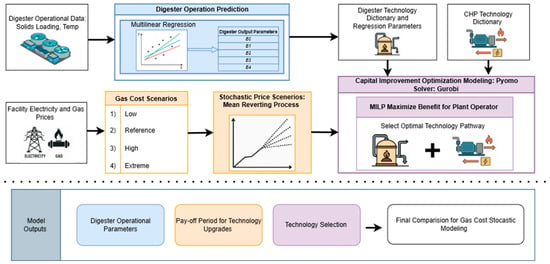
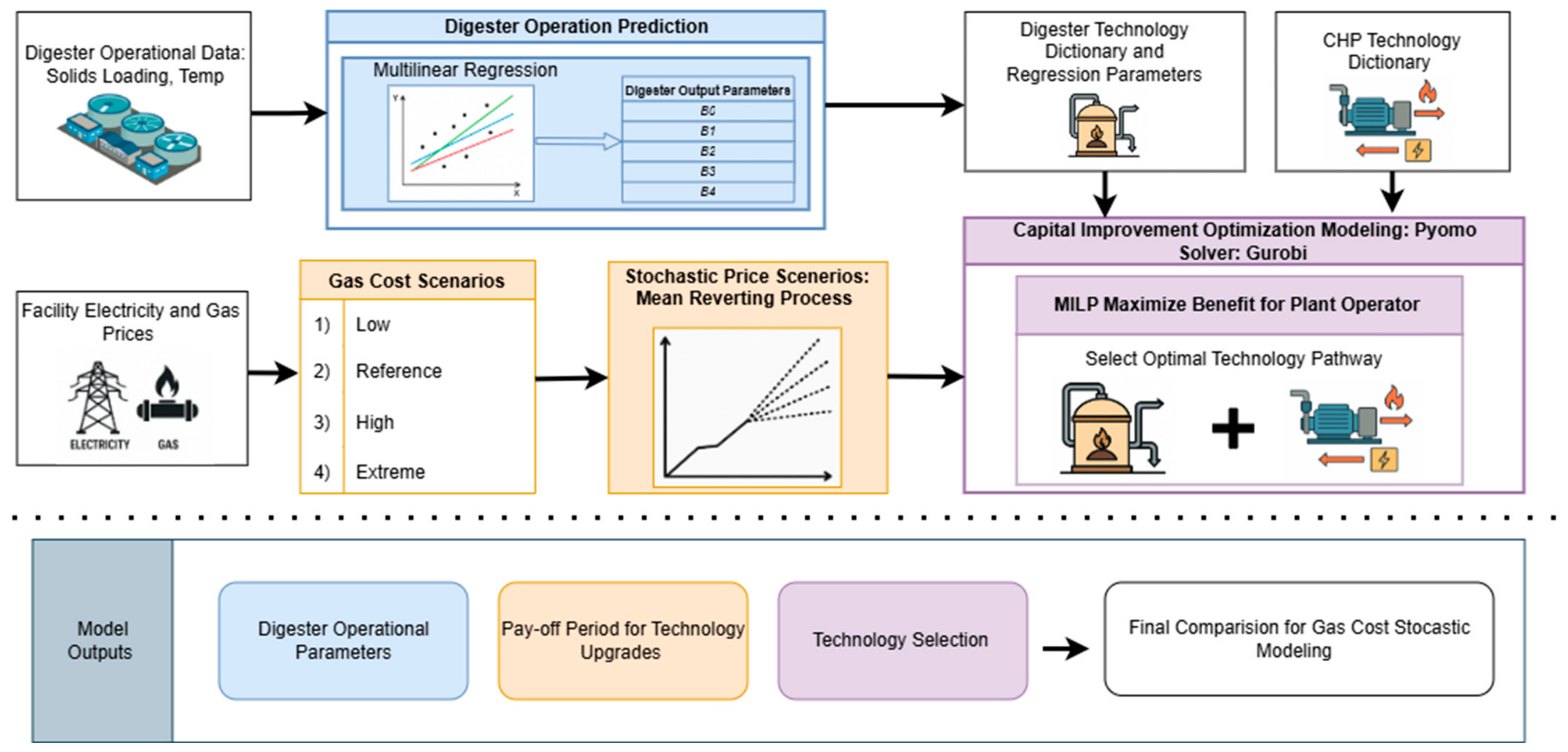
The suggested framework (Figure 1) links plant-specific biogas prediction simulated natural-gas prices, and economic optimization. Historical digester records are used to estimate regression coefficients, which parameterize biogas production within the optimization model. Technology performance and cost inputs are then combined with simulated prices to evaluate CHP selection and digester operating conditions. Outputs include selected technologies, modeled energy recovery, economic benefit, and payback estimates. These outputs identify alternatives that warrant further site-specific assessment under the stated assumptions. Here is a breakdown of how the framework functions: (i) The Digester Operation Prediction (The “Supply-side”) in the top-left track focuses on predicting how much biogas a facility can produce based on its operational reality via multilinear regression which generates specific regression coefficients that define the efficiency of the current digester technology; (ii) Economic & Stochastic Modeling (The “Market” Side) in the bottom-left track accounts for the volatility of energy markets, which is critical for calculating return on investment that uses a stochastic autoregressive process for energy prices that captures temporal dependence and price variation over time [24]; (iii) Capital Improvement Optimization (The “Decision” Engine) where the physical technology meets the financial data to find the best path forward as it pulls data on available biogas production and CHP technologies, including their costs and performance specs, and then runs a Mixed-Integer Linear Programming (MILP) model to maximize the benefit for the plant operator. The framework evaluates various technology upgrade combinations to identify the pathway that maximizes net profit or minimizes operational costs within predicted gas price scenarios. The resulting model outputs provide stakeholders with actionable insights, including optimized digester operational average parameters, estimated payback periods for energy savings, and specific technology selection recommendations. By offering a final comparison across volatile price futures, this tool acts as a screening step into economic pathways.

Figure 1. Integrated predictive–stochastic optimization framework for digester and CHP technology selection.

2.1. Biogas Prediction

Regression Model Formulation

Multilinear regression (MLR) offers a simple yet effective and widely used approach for predicting biogas yield, supporting preliminary energy and economic assessments. Reviews show that MLR commonly uses feedstock composition, loading rates, and operating conditions and achieves strong predictive performance, although slightly below advanced machine learning models [25]. Biogas optimization frameworks use prediction models to identify performance-maximizing conditions under real-world constraints, and a review of 55 studies shows that temperature, pH, retention time, pretreatment, and organic loading rate are among the five key factors driving biogas optimization [26]. Accordingly, MLR was used to relate biogas production to a limited set of operational and temporal predictors relevant to digester performance.

For model parsimony and interpretability, the regression included digester temperature, organic loading rate (OLR_t), lagged biogas production to represent temporal dependence, and paired sine and cosine terms to represent annual seasonality while allowing the seasonal phase to vary [27,28,29].

$$\begin{gathered} \widehat{y_t}={\mathsf{\beta }}_0+{\mathsf{\beta }}_1{\mathit{OLR}}_t+{\mathsf{\beta }}_2{B}_{\left(t-1\right)}+{\mathsf{\beta }}_3{\mathit{temp}}_t+{\mathsf{\beta }}_4\sin \left(\left(2\mathsf{\pi }/12\right){\mathit{Month}}_t\right) \\ +{\mathsf{\beta }}_5\cos \left(\left(2\mathsf{\pi }/12\right){\mathit{Month}}_t\right)+{\mathsf{\epsilon }}_t \end{gathered}$$

(1)

The subscript t denotes the time step, with each variable evaluated at day (t). Specifically, (ŷ_t) represents the predicted biogas production at time t, while (OLR_t) denotes the organic loading rate at the same time step. The term (B_t−1) represents biogas production from the preceding prepared observation and is included to capture temporal persistence in the digestion process. Similarly, temp_t denotes the digester operating temperature at time t, reflecting its influence on microbial activity. Finally, Month_t represents the calendar month corresponding to time t, and the paired seasonal terms sin[(2π/12) Month_t] and cos[(2π/12)Month_t] represent annual seasonal variation while allowing the seasonal phase to vary. Additional information on regression design and diagnostics can be found in Supplementary Materials.

In this study, biogas production refers to the total volume of digester gas (ft³/day), methane content refers to the volumetric methane fraction of the biogas (F^H_i,t), and methane production refers to the methane volume, obtained as the product of biogas production and methane content.

The regression model is intended to be calibrated separately for each wastewater treatment plant rather than transferred directly using coefficients estimated from the present case study. Application at another facility requires plant-specific historical operating data prepared using the same data structure and preprocessing procedures described in this study. The facility-specific dataset is then used to estimate its own regression coefficients before integration with the optimization framework. This approach allows the predictive component to reflect differences in digester configuration, feed characteristics, operating conditions, and process performance among facilities. Therefore, the framework is transferable in structure, while the fitted biogas-production model remains site-specific.

2.2. Biogas Benefit Maximization

The biogas benefit model is a MILP with the ability to select technology options for the optimal technology pathways to maximize benefits for the plant operator. We define the model objective function as a benefit-based maximization that captures the avoided costs of natural gas, electricity, and on-site power produced by the selected CHP system, thereby representing the net economic benefit to the plant operator. We identify the benefits of economic investment based on the avoided cost of electricity and natural gas. These benefits are directly related to the volume of gas produced by the digestion process. By including the biogas operation in the model, we can optimize benefits within operational limits and by selecting CHP (SelC_c,) technology pathways using a MILP. The costs estimated in the objective function are based on the net power (NP_c), a parameter of the CHP technology (c), and biogas (Biogas_t,y) volume from each of the digesters (i) in operation. Variable and Parameter are indexed by daily (t) or monthly (m) time steps, and over the lifetime of the technology in years (y). The benefit-maximization objective is shown in Equation (2), which defines (Z) as the benefit to be maximized over each major cost group.

The technology set C also includes a “No Investment (Flare)” alternative with zero net power and, therefore, zero CHP capital, installation, scrubber, and O&M costs (Table 2). This alternative represents the baseline of continued flaring under the observed digester operation and incurs the same digester operating costs as the CHP alternatives. Because exactly one alternative must be selected (∑ SelC_c = 1), a CHP technology is chosen only when its objective value exceeds that of continued flaring, and the incremental benefit of a CHP alternative relative to the baseline is ΔZ = Z_CHP − Z_flare. Each CHP alternative represents a new installation priced with the full equipment, installation, and scrubber costs in Table S3. The two existing CHP units at the case-study facility are assumed to remain idle and are treated as sunk; no salvage, recommissioning, or decommissioning costs or credits are included, and the existing gas-cleaning infrastructure is not credited.

Table 2. Abbreviated CHP technology dictionary name and net power.

CHP System (c)	Net Power kW (NPc)
Reciprocating Engine 35 kW	34.7
Reciprocating Engine 100 kW	99
Reciprocating Engine 250 kW	247.5
Reciprocating Engine 500 kW	495
Reciprocating Engine 1 MW	990
Reciprocating Engine 2 MW	1980
Reciprocating Engine 3 MW	2970
Reciprocating Engine 4 MW	4455
Gas Turbine 2 MW	1980
Gas Turbine 3.5 MW	3470
Gas Turbine w/Duct Burner 2 MW	1980
Gas Turbine w/Duct Burner 3.5 MW	3470
Microturbine 65 kW	61
Microturbine 200 kW	190
Microturbine 600 kW	570
Microturbine 1 MW	950
No Investment (Flare)	0

SelC_c ∈ {0, 1} is the only binary variable, and the model contains no general-integer variables. Digester OLR, temperature, and biogas production; storage level, injection, and withdrawal; flared gas; recovered and waste heat; avoided electricity and natural gas; and the soft-bound slack variables are continuous variables. All other quantities, including net power, fuel input, operating hours, efficiencies, methane content, digester feed flow, influent temperature, physical properties, costs, and prices, are fixed parameters (see Nomenclature Section). Consequently, every product in Equations (2)–(10) is a parameter multiplied by either a continuous or a binary variable; no product of two decision variables occurs, no linearization is required, and the model is represented as a MILP.

$$\begin{gathered} \mathit{max} Z=-\sum _{c\in C}{\mathit{CapCosts}}_c+\sum _{y\in Y, c\in C}({\mathit{AvoidedEmissions}}_c-{\mathit{AddCost}}_c) \\ +\sum _{y\in Y, t\in T}({\mathit{AvoidedCost}}_{t,y}-{\mathit{BioOMCost}}_t)-\sum _{y\in Y, t\in T, c\in C}{\mathit{OMCost}}_c \\ -\sum _{y\in Y, t\in T, i\in I}{\mathit{BioOPCost}}_{t,i}+\sum _{y\in Y, m\in M}{\mathit{AvoidedDemand}}_m \end{gathered}$$

(2)

The model is solved as a single MILP over the full 20-year planning horizon. Capital costs are incurred once; daily terms are summed over t ∈ T and y ∈ Y using the corresponding day of each simulated price trajectory (monthly AR(1) prices expanded to a 365-day calendar); monthly demand savings are summed over m ∈ M and y ∈ Y; and the technology-level terms AvoidedEmissions_c and AddCost_c are counted once per year. OMCost_c (Equation (4)) is evaluated per day and summed over all days of the horizon. All costs and natural-gas prices are expressed in constant 2016 dollars (real terms); therefore, no general inflation or price escalation is applied, and O&M costs and demand charges are held constant in real terms.

We further break down the objective function in Equations (3)–(10) into three general categories: capital and O&M costs associated with the CHP system, O&M costs associated with the biogas technology and avoided costs due to CHP installation. The costs associated with installation and operation of the CHP system are related to the installation costs (I_c), CHP system costs (E_c), scrubber costs (S_c), additional fuel cost for equipment such as duct burners (AC_c), and operations and maintenance costs for the CHP system (O_c) and scrubber (OS_c). These are shown below in Equations (3)–(5) for a particular year. Associated costs for CHP and biogas systems are detailed in Supplementary Materials and represent 2016-dollar values.

CapCosts_c = NP_c(I_c + E_c + S_c) SelC_c

(3)

OMCost_c = NP_c(O_c + OS_c)SelC_c

(4)

AddCost_c = NP_c AC_cSelC_c

(5)

The cost benefit is calculated in avoided cost expressions based on natural gas (${A^{\mathit{NG}}}_t$), demand (DC), and electricity (${A^E}_t$) avoided costs per unit. We added the additional option for cost benefit to avoid CO₂ emissions based on avoided emissions (${A^C}_c$) and associated cost of emissions (EV). Equations (6)–(8) are the objective function items related to the benefit of the operator they relate to an avoided cost based on the installation of a CHP system. Natural-gas prices NCt,y are expressed in $/ft³ (the simulated $/Mcf price divided by 1000); electricity prices ECt,y follow Equation (24) in Section 2.3.

$${\mathit{AvoidedCost}}_{\mathit{ty}}={A^E}_t {\mathit{EC}}_{t,y}+{A^{\mathit{NG}}}_t{\mathit{NC}}_{t,y}$$

(6)

$${\mathit{AvoidedDemand}}_m=\mathit{DC} \sum _{c\in C}{\mathit{NP}}_c {\mathit{SelC}}_c$$

(7)

$${\mathit{AvoidedEmissions}}_c={A^C}_c \mathit{EV} {\mathit{SelC}}_c$$

(8)

This shows costs associated with biogas costs for violating soft operation limits for digester temperature $(P_b^{\mathit{temp}}$) and OLR ($P_b^{\mathit{OLR}}$) for biogas production. Equation (9) is associated with the digester technology operation. Equation (10) adds a digester O&M cost proportional to facility biogas production, where the digester O&M cost per unit of biogas is c^OM.

$${\mathit{BioOPCost}}_{t,i,b}=[P_b^{\mathit{OLR}} \ast ({\mathit{OS}}_{i,t }^{+}+{\mathit{OS}}_{i,t}^{-})+P_b^{\mathit{temp}}\ast ({\mathit{TS}}_{i,t }^{+}+{\mathit{TS}}_{i,t}^{-}\left)\right]$$

(9)

BioOMCost_t = c^OMBiogas_t

(10)

The critical constraint for this program is the energy balance equation. The constraint balances the biogas selection from the digester scenario, gas withdrawn from storage (FS_t,y), and heat (H^CH4) content with the fuel utilized by the CHP (${I^F}_c$), operating hours (Hr), and any excess gas that will be flared (F_t) or can be injected into storage (−TS_t,y).

$$({\mathit{Biogas}}_{t,y}-T{S}_t+F{S}_{t,y})H^{\mathit{CH}4}=\sum _{c\in C}{I^F}_c\mathit{Hr} {\mathit{SelC}}_c+F_t \forall t\in T, \forall y\in Y$$

(11)

We ensure a storage balance by utilizing a storage equation; each day’s gas storage level (SL_t,y) equals the day before minus withdrawal and plus injections and limited by the maximum storage (MS) available at the facility. The storage level is bounded by 0 ≤ SL_t,y ≤ MS. The initial storage level equals the storage capacity (SL⁰ = MS; Equation (14)), and the level on the last day of each year is carried over to the first day of the following year (Equation (15)).

SL_t,y = SL_t−1,y + TS_t,y − FS_t,y

(12)

SL_t,y ≤ MS

(13)

SL_0,1 = SL⁰

(14)

SL_0,y = SL_|T|,y−1, ∀y ∈ Y, y > 1

(15)

The avoided natural gas use (${A^{\mathit{NG}}}_t$) expressed in ft³/day and electricity produced by the system (${A^E}_t$), expressed in kWh, are calculated based on the selected technology. The equations for these variables are detailed in Equations (16) and (17) respectively. The avoided natural gas is calculated based on the recovered heat (${R^H}_t$) and efficiency of the boiler operating on biogas (η^BIO) divided by the heat rate of natural gas (H^NG) and efficiency of the boiler operating on natural gas (η^NG). The electricity produced by the system is based on the operational hours and the selected technology’s net power. Natural-gas heat content varies with gas composition [30]; the fixed gas heat-content assumptions used in this model are reported in Table S2.

$${A^{\mathit{NG}}}_t={\displaystyle \frac{ {R^H}_t {\eta }^{\mathit{BIO}}}{H^{\mathit{NG}} {\eta }^{\mathit{NG}}}}$$

(16)

$$\sum _{c\in C}{\mathit{NP}}_c \mathit{Hr} {\mathit{SelC}}_c={A^E}_t\forall t\in T$$

(17)

The recovered heat from the CHP system is determined by the thermal efficiency (${{\eta }^{\mathit{TH}}}_c$) of the technology and fuel input and is equal to the waste heat (${W^H}_t$), for heat produced but unable to be utilized, and recovered heat (${R^H}_t$), that is available to be reused in digesters and can offset boiler usage.

$$\sum _{c\in C}{{\eta }^{\mathit{TH}}}_c{I^F}_c\mathit{Hr} {\mathit{SelC}}_c={R^H}_t+{W^H}_t \forall t\in T$$

(18)

The recovered heat is constrained by heat demand at the plant, estimated using the heat transfer equation simplified from [31]:

$${R^H}_t \le \mathit{Flow} {\rho }^s C{p}^S\left({\mathit{TempOut}}_t -{\mathit{TempIn}}_t \right) \forall t\in T$$

(19)

$$Q=\dot{m}{c}_p∆T$$

(20)

with heat transfer in the related function (Equation (20)) being (${R^H}_t$), mass flow rate being the flow into the digesters (Flow) multiplied by density of water (ρ^s), specific heat (Cp^S) and delta T being influent temp (TempIn_t) and digester operating temp (TempOut_t). The recovered heat can be used to estimate the avoided natural gas costs using the boiler efficiency relation between natural gas (η^NG) and biogas (η^BIO), and the gas heat content (H^NG).

Biogas quantity per time and technology is based on the linear regression equation. We determine the associated regression parameters from the previous step (β₀, β₁, …, β₅), the initial biogas production for time step zero (B) to parameterize the biogas production by digester, the cosine t (c_t) and sine t (s_t) of the monthly variation.

B_i,t = β_i + β1_i ∗ OLR_i,t + β2_i ∗ B_{i, t−1} + β3_i ∗ temp_i,t + β4_i ∗ c_t + β5i ∗ s_t

(21)

The range of the temperature (temp_i,t) and OLR (OLR_i,t) are subject to soft and hard bounds set by those associated with the biogas technology. We introduce a slack variable associated with the temperature (${\mathit{TS}}_{i,t }^{+},{\mathit{TS}}_{i,t}^{-})$ and OLR (${\mathit{OS}}_{i,t }^{+}+{\mathit{OS}}_{i,t}^{-}$); these slack values are associated with the range outside of the soft bounds that incur an additional operational cost. Equations related to these soft bounds are located in the Supplementary Materials.

To determine system biogas production at each time step, the individual digestion of biogas production is summated. A weighted summation is used to determine the total system of methane production from the individual production and a mean temperature of the digesters is used as the digester operating temp (TempOut_t) for Equation (8); these are detailed in Supplementary Materials. Equations (2)–(21) make up the fundamental constraints and benefit-maximization model which maximize the benefit to the operator by selecting the cost optimal upgrade based on facility-provided operating conditions and capacities.

To determine the economic payoff period for CHP investments the formula below (Equation (22)) was implemented, determining the economic payoff over time. In the model a discount rate of 0% is applied to the payoff period equation. The discount rate effect on the payoff period (Payoff_t,y) is determined during post-processing and addressed in the Supplementary Material; therefore, the discount rate does not contribute to the objective modeling or decision making.

$$\begin{gathered} {\mathit{Payoff}}_{t,y}={\mathit{AvoidedCost}}_{t,y}+{\mathit{AvoidedDemand}}_{m\left(t\right)}-{\mathit{BioOMCost}}_t \\ +\sum _{c\in C}({\mathit{AvoidedEmissions}}_c-{\mathit{OMCost}}_c-{\mathit{AddCost}}_c-{\mathit{CapCosts}}_c) \end{gathered}$$

(22)

Full documentation for objective function, expression and constraints for benefit-maximization model formulation is located in Supplementary Materials. The model was implemented in Python (version 3.12.3) using Pyomo (version 6.9.5) and solved with the HiGHS (version 1.15.1) MILP solver (appsi_highs interface) with its default settings, including a relative MIP-gap tolerance of 10⁻⁴. Each run contains 39,923 variables (28 binary and the remainder continuous) and 31,100 constraints and solution time was approximately 70 s per run in average.

2.3. Economic and Stochastic Modeling

The cost variation of natural gas plays a large role in the benefit analysis of the CHP system [16] as it shows a relationship between gas costs and installation of CHP systems. Stochastic commodity-price models commonly incorporate temporal dependence and mean-reverting behavior to represent price variability over time [24]. For natural gas, autoregressive time-series models provide a computationally simplified approach for representing price dynamics, with AR(1) processes providing a discrete-time representation of mean-reverting behavior under the assumption of constant assumptions [32]. This allowing for the implementation of price scenarios through definition of mean values as a core of the stochastic price model. The stochastic price modeling utilizes first-order autoregressive process to estimate monthly gas prices for benefit model inputs. The process is calibrated using EIA historical industrial natural prices beginning in 2008–2026. Historical gas prices were converted to 2016 dollars using the Consumer Price Index for All Urban Consumers (CPI-U) [33,34] with the 2016 annual average CPI used as the reference year for inflation adjustment. This conversion places historical gas prices on a consistent real-dollar basis before calibration and scenario generation. The data is calibrated using an 80% sample data and 20% hold out sample. An autoregressive model of order one [AR(1)] was estimated using the calibration period, with a constant term and one lag. Four economic gas-price scenarios were established from the empirical distribution of historical calibration-period prices. The low, reference, high, and extreme scenarios were defined using the 25th, 50th, 75th, and 95th percentiles, respectively.

To determine the simulated gas cost at each time step (X_t), the estimated AR(1) (φ) persistence parameter and empirical innovation distribution were held constant across scenarios, while the long-run mean (μ_s) was shifted to the corresponding historical percentile. At each time step, an innovation (ϵ_t) was randomly sampled (random seed: 42) with replacement from the empirical distribution of historical AR(1) residuals. Thus, the scenarios isolate the effect of alternative long-run gas-price environments while retaining a common representation of short-term price persistence and historical stochastic variability. The simulated gas price at each time step is given by (23):

X_t = μ_s + φ(X_t−1 − μ_s) + ϵ_t

(23)

Monthly gas prices generated by the AR(1) model are expanded to a daily 366-day calendar for each year of the 20-year horizon. Electricity prices are linked to the simulated natural-gas prices as (24), where EC₀ and NC₀ are the facility’s base electricity and natural-gas prices (Table S2) and ρ_r = 0.87 is the natural-gas-to-electricity price correlation factor for the Mid-Atlantic region.

EC_t,y = max{EC₀[1 + ρ_r(NC_t,y − NC₀)/NC₀], 10⁻⁴}

(24)

In this work, the avoided cost of the technology paths is dependent on the cost futures of natural gas and electricity; hence, the benefit-maximization model aims to find the optimal cost benefit selection for the input gas and energy cost. We then represent gas prices in a stochastic, time-varying process over a technology’s operational lifetime.

3. Case Study

3.1. System Description

A Wastewater Treatment Plant (WWTP) with an average treatment capacity of 55 million gallons per day was selected as the case study. The plant co-digests primary sludge, thickened waste-activated sludge, and FOG. In this system, feedstock undergoes THP to enhance biodegradability before being fed into three anaerobic digesters, where higher loading rates enable microbial conversion to biogas with increased methane yields and greater volatile-solids reduction. The facility opted to implement THP rather than construct an additional digester a few years ago, as cost analysis indicated that THP was approximately 50% more economical. Although the plant has two CHP units installed to utilize this biogas, their operation remains limited for years now; according to all plant records, biogas is flared. The THP digestion configuration has substantially reduced the volume of biosolids requiring disposal, but its potential for renewable energy generation has not yet been fully leveraged.

3.2. Data and Constraints

The research uses daily plant operational data (January 2022–December 2024), including flow of biosolids fed to the digester, OLR, produced biogas volume, biogas composition, temperature, and energy consumption, to calibrate a biogas prediction model. Each digester has a constant working volume of 1.13 million gallons with daily operational changes restricted using ramping limits based on the plant recommendation of ±1% for OLR, and ±2.5 °F for temperature, ensuring that no variable could shift more than these amounts from the previous day’s value. Digester temperature was recorded and modeled in degrees Fahrenheit. For the optimization model, the allowable range was set at 95–110 °F (35.0–43.3 °C), representing the plant’s historical operating regime while limiting extrapolation beyond observed conditions. Approximately 99.9% of valid temperature observations fell within this range, with values concentrated near 105 °F. The broader 60–150 °F interval was used only as a preprocessing plausibility filter and did not represent an operating constraint. Operators clarified that temperature is governed by cooling limitations after THP and can routinely reach as high as 106–110 °F. OLR was constrained by hard bounds of 0.156–0.317 and soft bounds of 0.179–0.269 lb VS/ft³/day (Table S2); deviations outside the soft bounds are penalized through the slack variables in Equation (9).

Energy billing records and unit-process operating sheets support evaluation of net energy recovery to quantify gains in biogas output, energy efficiency, and cost performance under different technology pathways and fuel price conditions. DOE CHP fact sheets were used to establish generalized capital, O&M, and additional costs, as well as technology efficiencies for three common systems: microturbines, reciprocating engines, and gas turbines [35]. Base-case natural gas and electricity prices were drawn from EIA industrial natural gas data [36] and power bills, with natural gas price variability represented using the standard deviation of annual industrial prices from 2008–2024.

3.3. CHP Technologies

For this case study, we have chosen the CHP technology options detailed in Table 2. The table summarizes net power outputs for various CHP technologies, showing that reciprocating engines and gas turbines deliver scalable outputs from tens of kW up to several MW (with near-rated efficiency), while microturbines provide smaller-scale power generation with slightly lower net outputs. The technical and cost parameters used in the optimization for each technology (equipment, installation, and scrubber costs; O&M costs; fuel input; electrical and thermal efficiencies; heat-recovery capacity; and emission rates) along with a full technology list are listed in Supplementary Table S3, and the facility inputs and model constants are listed in Table S2. The “No Investment (Flare)” alternative represents continued flaring with no CHP capital or O&M costs.

3.4. Gas Prices

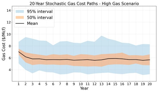
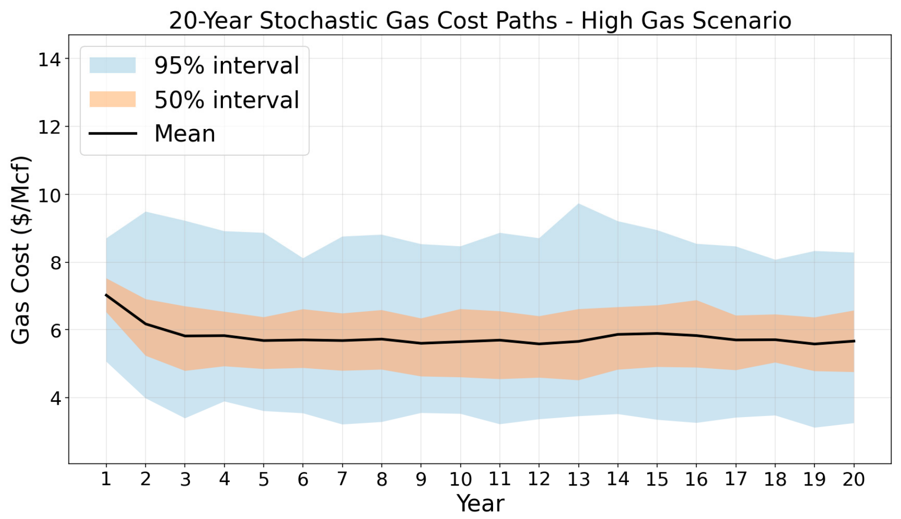
The stochastic gas-price model described in Section 2.3 was applied to generate gas-price realizations for the 20-year economic analysis shown in Figure 2. Four counterfactual gas-price environments were evaluated: Low, Reference, High, and Extreme. These scenarios correspond to the 25th, 50th, 75th, and 95th percentiles, respectively, of the historical calibration-period natural-gas price distribution and are shown in Table 3. Within each scenario, stochastic price trajectories were generated using the common AR(1) persistence and empirical innovation distribution described in Section 2.3, while the scenario-specific long-run price level was varied.

Figure 2. Gas prices for high scenario displaying stochastic variation over 20-year lifecycle. Prices are expressed in 2016 dollars per thousand cubic feet ($/Mcf). The scenario-specific long-run price level is $5.44/Mcf.

Table 3. Gas cost scenario descriptions.

	Gas Cost Scenario	Gas Cost ($/Mcf)
(1)	Low Gas	3.79
(2)	Reference	4.56
(3)	High	5.44
(4)	Extreme	9.32

The resulting gas-price trajectories were incorporated into the economic optimization model to evaluate technology-selection outcomes under alternative gas-price conditions. Multiple stochastic realizations were evaluated within each scenario to capture variation in the economic conditions experienced by the modeled facility. The resulting simulations provide a basis for comparing the consistency of modeled technology selections and economic outcomes across alternative long-run gas-price environments.

4. Results and Discussion

Traditionally, municipalities have addressed increasing solids loading by constructing additional anaerobic digesters; however, this approach involves high capital costs, larger physical footprints, and persistent limitations due to slow digestion kinetics. In contrast, intensification technologies such as THP aim to overcome these constraints by enhancing hydrolysis, enabling higher organic loading rates, improving process stability, and reducing required retention times. THP can be a cost-effective option for achieving higher capacity, improved solids destruction and collecting methane within existing infrastructure [37]. Nevertheless, although THP is a technologically mature process, its adoption in the United States remains relatively recent and limited, and it requires significant upfront capital investment. In an industry article published on 4 June 2025, Greseth reported nine thermal hydrolysis plants were in operation in the United States [38]. Therefore, there is limited research on its integration with CHP systems in the United States. THP improves digestion capacity and can avoid new digester construction, especially in large plants [39]. It is most economically attractive for medium- to large-scale WWTPs, typically those treating flows on the order of ≥50 MGD, where economies of scale allow the capital and energy requirements to be offset by gains in biogas production and solids reduction; however, recent developments indicate that smaller, high-solids systems are increasingly becoming feasible [7]. This study contributes to an evolving discussion on the potential benefits of coupling THP with CHP. Continued research in this area may provide additional incentives for facilities to adopt THP by enhancing its economic viability through improved energy recovery and biogas utilization.

The findings of this study are consistent with the existing literature emphasizing the importance of process optimization and intensification in improving the economic viability of anaerobic digestion systems and have shown that while biogas production is a promising renewable energy pathway, it often struggles to remain cost-competitive with conventional natural gas without technological improvements or favorable economic conditions [40]. In this context, the present study extends the literature by introducing an integrated framework that combines process prediction, stochastic economic modeling, and optimization to evaluate infrastructure upgrade strategies under uncertain energy prices. This highlights the importance of incorporating uncertainty into infrastructure planning, rather than relying solely on deterministic or average-case economic assumptions.

4.1. Biogas Prediction Results

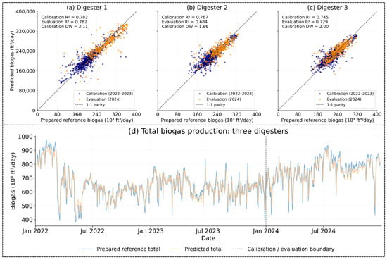
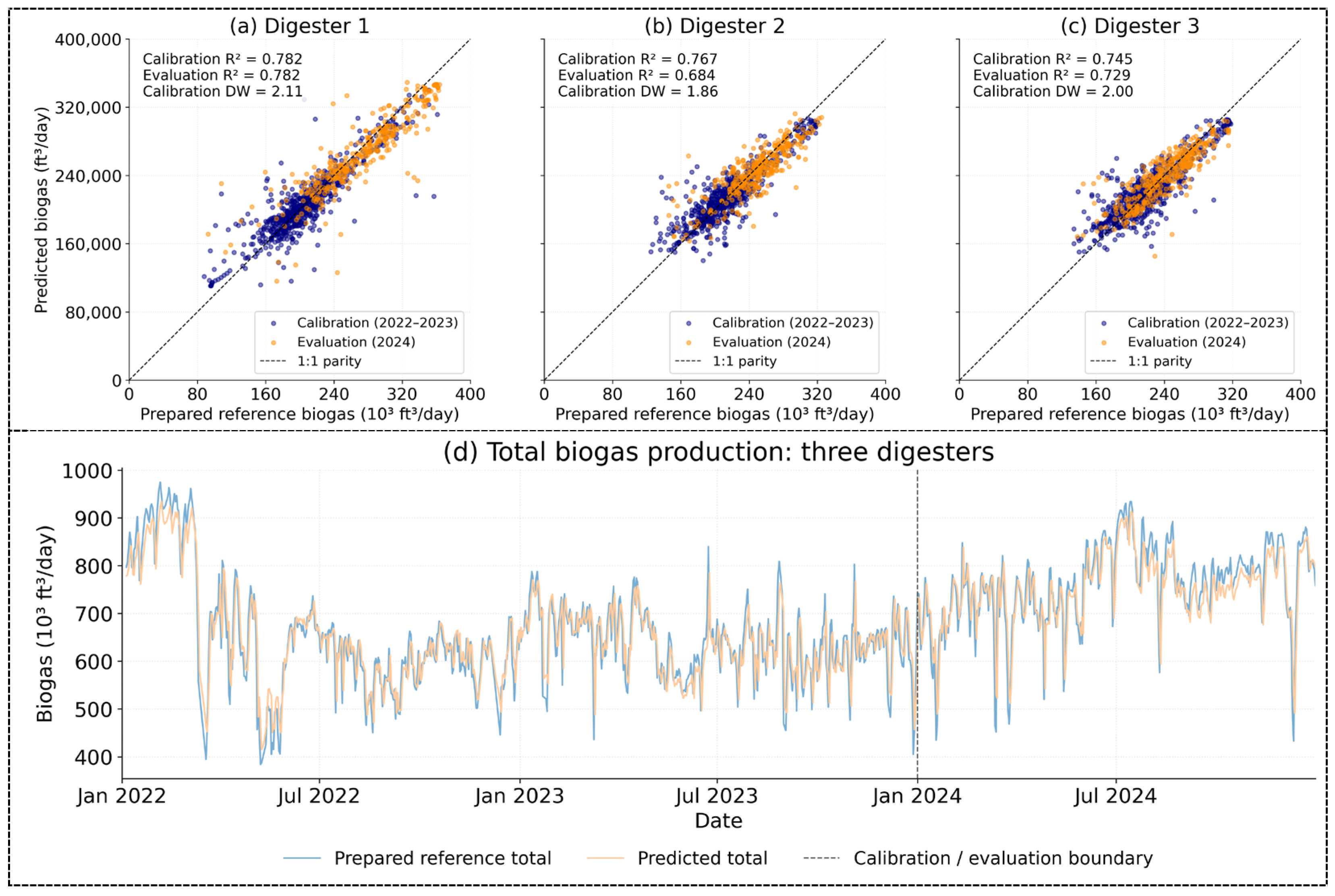
Separate multilinear regression models were developed for the three digesters using 2022–2023 records and evaluated against the prepared 2024 biogas-production series. Model performance was generally consistent across digesters. Calibration R² values ranged from 0.75 to 0.78, while 2024 R² values ranged from 0.68 to 0.78. MAPE remained below 7% for all digesters in both periods, with 2024 values ranging from 5.58% to 6.74% (Table 4). Overall, the models reproduced a substantial portion of the day-to-day variation in the prepared biogas-production series, although performance varied somewhat among digesters. Figure 3 presents model performance at both the digester and facility levels. Each digester panel includes all 366 prepared 2024 observations. The facility-level series represents the sum of the three digesters on dates common to all models. For 2024, the facility comparison included 363 dates and yielded R² = 0.70, RMSE = 48,378 ft³/day, and MAE = 35,289 ft³/day. These aggregate results complement the digester-specific evaluation by characterizing overall agreement between predicted and prepared facility-level biogas production.

Table 4. Calibration, 2024 evaluation, and residual diagnostics of the digester regression models. Note: RMSE and MAE are expressed in ft³/day. Residual diagnostics refer to the 2022–2023 calibration residuals. DW = Durbin − Watson; BP = Breusch − Pagan; BG = Breusch − Godfrey. Values below 0.01 are reported as <0.01 rather than 0.00.

Digester	Period	n	R2	RMSE (ft3/day)	MAE (ft3/day)	MAPE (%)	BP p	BG-7 p	BG-30 p
DIG1	2022–2023 Calibration	726	0.78	19,889.10	12,869.60	6.79	0.58	0.63	0.02
DIG1	2024 Evaluation	366	0.78	23,844.20	16,240.30	6.74	—	—	—
DIG2	2022–2023 Calibration	726	0.77	17,210.00	12,152.60	6.00	<0.01	0.01	<0.01
DIG2	2024 Evaluation	366	0.68	18,876.50	13,379.90	5.74	—	—	—
DIG3	2022–2023 Calibration	726	0.75	18,154.70	13,300.40	6.32	<0.01	0.90	<0.01
DIG3	2024 Evaluation	366	0.73	17,637.30	12,646.50	5.58	—	—	—

Figure 3. Evaluation of the MLR model. (a–c) Observed-versus-predicted biogas production for Digesters 1–3, with colors distinguishing the 2022–2023 calibration period from the 2024 evaluation period. (d) Facility-level prepared and predicted biogas production from 2022 to 2024, obtained by summing the three digesters on common valid dates. The boundary between the calibration period and the 2024 evaluation period is indicated.

Residual diagnostics indicated Durbin–Watson values close to 2 for all models. However, the Koenker–Breusch–Pagan test indicated heteroskedasticity for DIG2 and DIG3, while the 30-lag Breusch–Godfrey test indicated longer-lag residual dependence in all three digesters. Coefficient uncertainty was therefore evaluated using Heteroskedasticity- and Autocorrelation-Consistent (HAC) standard errors with a Bartlett kernel, a 21-record lag, and finite-sample correction. Lagged biogas coefficients ranged from 0.779 to 0.817, indicating substantial temporal persistence. Paired sine and cosine terms were retained to represent annual seasonality, with joint HAC p-values of 0.026, 0.019, and 0.147 for DIG1–DIG3, respectively. OLR and Temperature associated with positive relationships aligning with expected biological kinetics [41]. We admit that MLR model R2 values of 0.686–0.784 perform slightly below advanced machine learning models such as those evaluated by Sun et al. (2023) [17]. Nevertheless, MLR was selected here for its simplicity and interpretability. Complete coefficient estimates and uncertainty measures are provided in Supplementary Table S1.

4.2. Economic and Stochastic Modeling Results

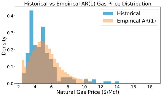
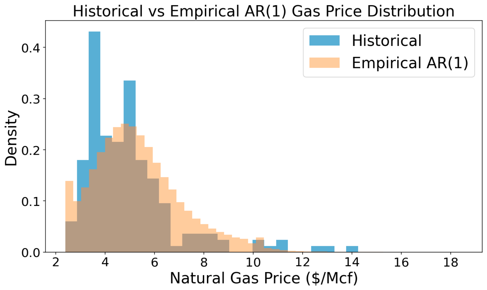
The historical natural gas price sample contained 220 observed values from January 2008 through June 2026, of which 176 data points were used for calibration and 45 data points were used for validation. The calibrated AR(1) model produced a persistence parameter of 0.919 and an innovative standard deviation of $0.711 per thousand cubic feet, with the simulated and historical price distributions compared in Figure 4. The estimated long-run mean of calibrated process was $4.83 per thousand cubic feet, while the minimum calibration price was $2.39 Mcf. The high persistence value observed demonstrates substantial temporal dependence in historical gas price series. Residual diagnostics indicated no statistically significant remaining autocorrelation through 12 lags.

Figure 4. Comparison of the historical natural-gas price distribution during the calibration period with the distribution generated by the calibrated empirical AR(1) model. Histograms are shown as probability densities to facilitate comparison of the observed and simulated price distributions.

The calibrated simulations reproduced several statistical characteristics of the calibrated data. Across the simulated trajectories, the mean gas price was $5.35 per thousand cubic feet compared with $5.01 in historical calibration period, while the historical standard deviation was $1.80 compared with $1.99 historically. The simulated median was $5.11 compared to the historical median of $4.66. The model reproduced the 10 percentiles with simulated ($3.23) with a −2.7% difference to historical ($3.32), while the upper percentile differences increased with 50 and 75 percentiles with 9.6% and 13.1% difference respectively. The 95 percentiles decreased to −1.0% difference between simulated and historical.

The 45 validation test prices showed greater differences from the observed data. For the 45-observation holdout, the historical mean and median were $3.75 and $3.45 per thousand cubic feet, respectively, compared with simulated values of $5.72 and $5.66. The simulated standard deviation was also higher, at $1.69, compared with $1.03 historically.

The out-of-sample results therefore indicate that the stochastic model should be interpreted as a scenario-generation framework rather than a point-forecasting model for future natural-gas prices. Its primary purpose in this study is to generate temporally correlated prices around specified long-run gas-price environments for economic screening. Consequently, economic results obtained from the stochastic scenarios are interpreted as conditional outcomes under alternative gas-price environments rather than predictions of future natural-gas prices.

4.3. Benefit Maximization

To evaluate the sensitivity of the CHP investment decisions to natural-gas price variability, 100 stochastic simulations were evaluated for each of the four gas-price scenarios, resulting in 400 simulation outcomes. Uncertainty in this analysis arises from the stochastic natural-gas price trajectories generated by the AR(1) price model; biogas production was not independently sampled as a stochastic variable. Therefore, the resulting variation in economic outcomes reflects differences in the energy-price trajectories applied to the modeled CHP pathways.

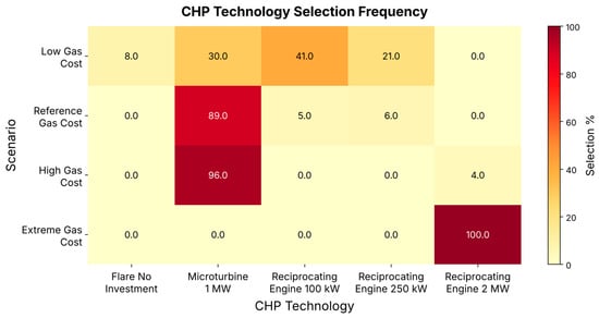
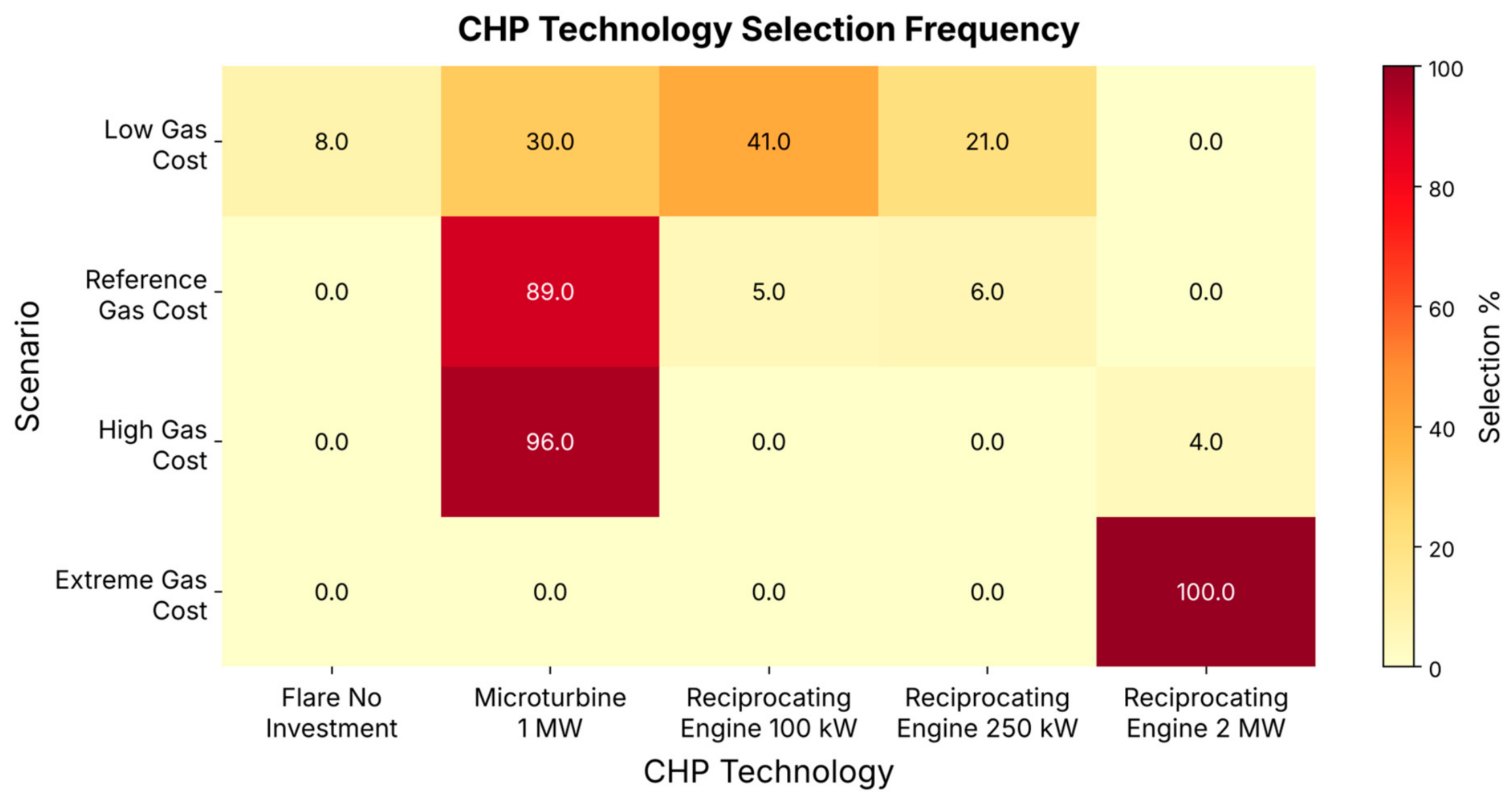
The resulting technology selections were aggregated and summarized in Figure 5, which shows the selection frequency for each scenario. The selection of technologies reflects the cost-effective pathways for quantity of gas produced and lowest capital costs and O&M cost related to operating engine with optimal economic return. Technology choices under the high and extreme gas cost scenarios were stable across the 100 runs. The reference gas cost and low gas cost cases show increased variability in the technology decisions. This variability signifies a region where marginal changes in gas costs create competition between the technologies.

Figure 5. Technology selection frequency across four stochastic natural gas cost scenarios, based on a sample size of 100 runs. Greater selection stability observed for CHP technologies under high and extreme gas cost conditions. Scenarios are ordered as in Table 5, Table 6 and Table 7.

While technology pathways can provide insight into the robustness of investment choices under cost uncertainties, the performance of each investment pathway can be evaluated through payback periods for each cost scenario. Table 5 compares the simple (undiscounted) payback period for each natural gas cost scenario. The results indicate that the modeled payback period was sensitive to the natural-gas price environment, with higher gas-price scenarios generally producing shorter payback periods.

The probability of achieving payback also varied substantially among scenarios. Payback occurred in all 100 Extreme Gas & Energy Cost simulations and 99 of 100 High Gas & Energy Cost simulations. In comparison, payback occurred in 74% of Reference simulations and only 15% of Low Gas & Energy Cost simulations. Across all 400 simulations, 72% produced a valid payback period. Thus, while the modeled CHP pathways frequently recovered their initial investment under higher gas-price conditions, payback was considerably less consistent under lower gas-price conditions. The mean final cumulative net benefit was $3.63 million under the Extreme Gas & Energy Cost scenario, compared with $0.73 million under the High scenario, $0.20 million under the Reference scenario, and −$0.17 million under the Low scenario. A negative net benefit indicates that the modeled savings did not recover the capital and operating costs, including digester operating costs.

The probability of a positive final cumulative net benefit was 100% for the Extreme scenario, 99% for the High scenario, 74% for the Reference scenario, and 15% for the Low scenario. Cumulative net benefit was also analyzed for each scenario; this measure allowed the economic benefit to be evaluated for runs in which payback was not achieved.

The technology-level results further illustrate the effect of energy-price uncertainty on modeled economic outcomes shown in Table 6. Across the selected CHP technologies, the 2 MW reciprocating engine exhibited a narrower payback range and positive final cumulative net benefit in all selected simulations, while the 1 MW microturbine showed greater payback variability and positive net benefit in 85.58% of selected simulations. The smaller reciprocating-engine alternatives and the flare/no-investment pathway produced negative final cumulative net benefits in all simulations in which they were selected with flaring representing the 20-year estimation of operating digesters within normal range with no production maximization.

Because the flare alternative is included in the selection set, the 100 kW and 250 kW reciprocating engines selected under the Low scenario were chosen only because their objective values were slightly less negative than continued flaring in those realizations (mean net benefits of −$254,953 and −$220,820 in the runs in which they were selected, compared with −$281,069 for flaring; Table 6). Their incremental benefit relative to flaring is therefore small, they did not achieve a positive net benefit within the 20-year horizon in any realization, and they should be interpreted as economically marginal outcomes rather than recommended investments.

Simple (undiscounted) payback periods in the primary analysis were calculated from the cumulative undiscounted payoff over the 20-year operating period. To assess the effect of the time value of money, supplemental analyses applied 5% and 10% discount rates during post-processing to the annual payoff streams. The resulting discounted payoff periods are reported separately in the Supplementary Material.

Table 5. Mean and range of the simple (undiscounted) payback period for the gas cost scenarios.

	Gas Cost Scenario	Mean Payback Period (yr)	Range (yr)	5th–95th Percentile
(1)	Low	>20	16.5–>20	17.23–19.86
(2)	Reference	18.9	14.1–>20	16.54–19.73
(3)	High	16.4	13.3–>20	14.38–18.90
(4)	Extreme	12.3	10.3–15.1	10.84–13.49

Table 5. Mean and range of the simple (undiscounted) payback period for the gas cost scenarios.

	Gas Cost Scenario	Mean Payback Period (yr)	Range (yr)	5th–95th Percentile
(1)	Low	>20	16.5–>20	17.23–19.86
(2)	Reference	18.9	14.1–>20	16.54–19.73
(3)	High	16.4	13.3–>20	14.38–18.90
(4)	Extreme	12.3	10.3–15.1	10.84–13.49

Table 6. Mean Payback Period and Net Benefit for technology selection.

CHP Technology Selection	Count All Scenarios	Mean Payback Period (yr)	Mean Net Benefit ($)	Probability Final Net Benefit (%)
Flare No Investment	8	>20	−281,069.29	0%
Reciprocating Engine 100 kw	46	>20	−254,952.69	0%
Reciprocating Engine 250 kw	27	>20	−220,819.83	0%
Microturbine 1 MW	215	17.4	416,654.41	85.6%
Reciprocating Engine 2 mw	104	12.4	3,546,366.28	100%

Table 6. Mean Payback Period and Net Benefit for technology selection.

CHP Technology Selection	Count All Scenarios	Mean Payback Period (yr)	Mean Net Benefit ($)	Probability Final Net Benefit (%)
Flare No Investment	8	>20	−281,069.29	0%
Reciprocating Engine 100 kw	46	>20	−254,952.69	0%
Reciprocating Engine 250 kw	27	>20	−220,819.83	0%
Microturbine 1 MW	215	17.4	416,654.41	85.6%
Reciprocating Engine 2 mw	104	12.4	3,546,366.28	100%

Higher gas cost scenarios lead to shorter payback periods due to the direct relationship between the avoided costs of electricity and energy and the benefit maximization. Although previous studies have shown potential payback periods of 5.7 years [16], this study analyzed a 2,000,000 cubic meter per year facility dependent on thermal demand met rather than specific technologies. It is important to note that the objective function in this study maximizes total net benefit and not minimizing potential payback period. The payback periods obtained in this study ranging from 12.4 to over 20 years across low to extreme natural-gas price scenarios are broadly consistent with the long investment-recovery timelines reported by Balasundaram et al. (2025) [23]. In their techno-economic assessment, the most economically favorable configuration (THP-AD with Bio-CNG (compressed biomethane made from upgraded biogas)) exhibited a 17-year payback period, despite achieving the highest net present value and internal rate of return.

Balasundaram et al. (2025) [23] actually evaluated THP-AD primarily from a scenario-based, steady-state framework that incorporates process-performance, microbial, techno-economic, and lifecycle assessment perspective, demonstrating that THP increases methane yield and volatile solids reduction and that downstream utilization pathways (CHP versus Bio-CNG)) strongly influence environmental and financial outcomes. In contrast, this work focuses less on maximizing absolute methane yield and more on decision-making under uncertainty. Additionally, rather than treating CHP and biogas utilization pathways as static scenarios, our framework explicitly captures day-to-day operational dynamics, temporal dependence in biogas production, seasonal variation, and volatile energy markets, which proved critical in determining whether CHP deployment remains economically robust across gas-price regimes. While Balasundaram et al. identify THP-AD with Bio-CNG as the most profitable pathway and THP-AD with CHP as environmentally optimal, our results show that even at facilities with THP already installed, economic viability of energy recovery remains highly sensitive to natural gas prices and operational constraints, helping explain why many full-scale WWTPs continue flaring biogas despite favorable process performance. Together, the two studies are complementary: Balasundaram et al. establish the technical and environmental potential of THP-AD systems, whereas this work advances the literature by embedding that potential within a real-world, uncertainty-aware decision framework.

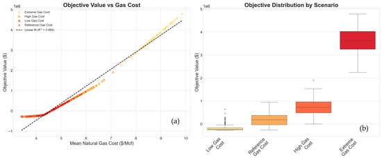
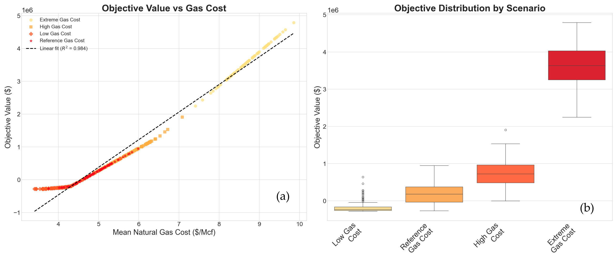
The objective function in Figure 6a exhibits an approximately linear (R² = 0.984) relationship with the cost of natural gas. Under low gas-cost conditions, the objective value remains negative in most stochastic realizations, leading to limited variation. In this region it selects the no-investment, 100 kw, 250 kw, and 1 MW CHP technology based on the benefit maximization (Figure 6). Even though our results as shown in Figure 6b agree with Tavakoli et al. (2021) [20] who showed that stochastic representation of electricity prices alters optimal CHP dispatch decisions, our results demonstrate that technology selection stability increases in higher natural-gas-price regimes. In the low gas-cost scenario, the mean objective value is negative; this behavior differs from the payback period metric because the objective function explicitly accounts for ongoing digester operation and maintenance costs. As gas cost increases, the distribution of objective values widens across scenarios.

Figure 6. (a) Correlation between objective function value and mean natural gas cost, presented as a scatter plot demonstrating an approximate linear relationship. (b) Distribution of objective function values by gas-cost scenario, indicating increasing variability as natural gas costs rise.

This increased spread reflects the stochastic natural-gas price trajectories, whose effect on avoided energy costs, and therefore on net benefits, is larger under higher gas-price conditions. Despite this variability, the selected technology configurations remain consistent, indicating that economic uncertainty primarily affects performance outcomes rather than technology choices as gas cost increases. Table 7 shows the numerical variability in the objective and the overview of model outputs for each scenario.

Table 7. Technology selection overview table.

	Gas-Cost Scenario	Total Samples	CHP Selection Distribution	Mean Objective	Mean Energy (kWH/YR)	Mean Heat (MMBtu/YR)
(1)	Low	100	Reciprocating Engine 100 kw: 41 (41.0%) Microturbine 1 MW: 30 (30.0%) Reciprocating Engine 250 kw: 21 (21.0%) Flare No Investment: 8 (8.0%)	$−165,397.43 ± $169,521.88	3,316,531	15,615
(2)	Reference	100	Microturbine 1 MW: 89 (89.0%) Reciprocating Engine 250 kw: 6 (6.0%) Reciprocating Engine 100 kw: 5 (5.0%)	$196,025.56 ± $276,681.49	7,600,795	34,489
(3)	High	100	Microturbine 1 MW: 96 (96.0%) Reciprocating Engine 2 MW: 4 (4.0%)	$728,048.80 ± $352,202.49	8,706,701	38,508
(4)	Extreme	100	Reciprocating Engine 2 MW: 100 (100.0%)	$3,625,963.21 ± $493,578.61	17,392,320	56,667

Table 7. Technology selection overview table.

	Gas-Cost Scenario	Total Samples	CHP Selection Distribution	Mean Objective	Mean Energy (kWH/YR)	Mean Heat (MMBtu/YR)
(1)	Low	100	Reciprocating Engine 100 kw: 41 (41.0%) Microturbine 1 MW: 30 (30.0%) Reciprocating Engine 250 kw: 21 (21.0%) Flare No Investment: 8 (8.0%)	$−165,397.43 ± $169,521.88	3,316,531	15,615
(2)	Reference	100	Microturbine 1 MW: 89 (89.0%) Reciprocating Engine 250 kw: 6 (6.0%) Reciprocating Engine 100 kw: 5 (5.0%)	$196,025.56 ± $276,681.49	7,600,795	34,489
(3)	High	100	Microturbine 1 MW: 96 (96.0%) Reciprocating Engine 2 MW: 4 (4.0%)	$728,048.80 ± $352,202.49	8,706,701	38,508
(4)	Extreme	100	Reciprocating Engine 2 MW: 100 (100.0%)	$3,625,963.21 ± $493,578.61	17,392,320	56,667

From the outputs we determined the heat recovery from our scenarios; this value is based on technology and usable heat. We can compare these values to Shen et al. (2015) [42] who determined the average estimated thermal energy in wastewater for all facilities across the United States was equal to 2.4 MMBtu/DAY per 1MGD. We compare this value to our 55 MGD facility and determine based on this scenario our thermal energy use is between 1.01 and 2.82 MMBtu/DAY per 1 MGD before thermal losses. THP has been shown to increase methane yield, leading to increased heat energy recovery. The mean electricity per year is not comparable to the previous paper as it is directly related to the CHP system selected.

4.4. Comparison Between the Case Study and the Proposed Optimization Model in Terms of Decision Making

The decision-making philosophy expressed by the case study’s real operation revealed a fundamental contrast with the strategy embedded in our framework. While our model prioritizes maximizing biogas production and selecting economically optimal technology pathways (e.g., CHP or pretreatment), the operators’ real-world focus is centered on biosolids-management economics rather than energy utilization, as most of the produced biogas is currently flared. The plant’s true operational priority is maximizing volatile solids reduction (VSR); higher VSR directly reduces biosolids’ hauling costs and mitigates long-term Per- and Polyfluoroalkyl Substances (PFAS) exposure risks. Biogas generation remains a secondary benefit, as only a small portion is used on site, and CHP, despite two installed units, is not economical due to siloxane removal costs, staffing needs, and limited heat integration with the THP system. Moreover, in terms of capital investment, operators emphasized that digester expansion must be avoided, with one digester always kept offline for maintenance and reliability. This implies that any optimization model must restrict feasible digester configurations accordingly and even consider scenarios with fewer digesters online with added pretreatment procedures, due to the economic burden of adding new digestion. In our case study, the plant has already invested nearly $50 million in pretreatment to avoid digester expansion, which would cost double that amount.

4.5. Limitations, Uncertainty and Future Research

Despite this work contribution, the study has several limitations. The modeling approach relies on simplified representations of biological processes as the regression model assumes linear relationships and relies on one-day lag, which may not fully capture nonlinear microbial behavior, and multi-day retention effects. Another limitation is that a key operator priority is maximizing VSR which we did not explicitly model.

Although research such as [16] suggest economic benefit and a payback period well within the 20-year lifetime, the real-world operation of these systems can be cost prohibitive to a plant operator. This suggests a gap in understanding the associated operations and maintenance costs and benefits of running a CHP system. A stronger analysis of the cost to wastewater facilities operating can reduce uncertainties in the economic viability of this benefit modeling. Additionally, in the benefit-maximization model, CHP is represented as a new installation that is selected only when it outperforms continued flaring, whereas in practice the existing CHP units are not used because of current economic and thermal-integration limitations. Therefore, any scenario assuming full CHP utilization should be interpreted as hypothetical unless the model explicitly includes its associated operating costs and heat-recovery constraints that make it possible to use it fully. All capital, operation, and maintenance cost parameters used in the benefit-maximization model are based on standardized 2016 cost estimates reported in the DOE CHP technology cost reference sheets, unless otherwise specified. Where facility-specific data were available, cost inputs were refined using values provided directly by the plant operator or the model user to better reflect local operational conditions. The use of 2016 cost data ensures internal consistency across technology options and aligns with widely cited public-sector cost benchmarks for CHP systems and energy equipment, providing a neutral basis for comparative evaluation of alternative technology pathways. Taken together, these insights show that the plant’s decision framework is fundamentally risk-averse, stability-driven, and biosolids-cost-minimizing, whereas our model remains in biogas recovery and reuse maximizing. The analysis is based on a single case study, which may limit the generalizability of the results across different wastewater treatment configurations and geographic contexts. Because the facility’s historical investment and operating decisions were not generated from the proposed optimization framework, the case study is intended as a retrospective decision-screening application rather than a prospective validation of the model’s ability to predict actual investment decisions.

Because all costs and natural-gas prices are expressed in 2016 dollars, the comparison is internally consistent in real terms; however, the CPI-U increased by approximately 31% between 2016 and 2024 [34], and CHP equipment and installation costs may have escalated faster than general inflation, which would lengthen the reported payback periods. A sensitivity analysis on capital and O&M costs is therefore recommended for future studies and before site-specific application. In addition, the model does not include the incremental staffing costs that operators identified as a barrier to CHP operation (Section 4.3); these costs may not be fully captured by the DOE non-fuel O&M values and would further reduce the modeled net benefits.

Future research should focus on integrating more detailed process-based models, expanding scenario analysis to include policy incentives such as carbon pricing, and validating the framework across multiple full-scale facilities. Additionally, it could incorporate operator-aligned objectives, particularly Volatile Solids Reduction (VSR) as a secondary objective. Further extensions could evaluate the economic benefits of Renewable Identification Number (RIN) credits for biogas utilization, pipeline injection options, and account for other constraints such as the high costs associated with scrubber maintenance, ensuring that the framework reflects both technical performance and real-world decision-making. A full exploration of the decision-making framework and comparison of selected technology pathways would further support the stability of the technology selection. The addition of smaller facilities without installed pretreatment would support the economic feasibility of installing CHP. The inclusion of a facility facing a capacity expansion decision would further validate the model’s formulation, showcasing the model’s ability to support technology pathway decisions.

5. Conclusions

The proposed integrated framework supports preliminary screening of CHP alternatives at WWTPs with THP already installed under simulated natural-gas price scenarios, with economic outcomes conditional on the modeled operating and cost assumptions. Further evaluation should incorporate operator priorities and site-specific operating costs and assess the framework across additional facilities. The literature indicates that CHP and other biogas-utilization pathways can provide economic and energy-recovery benefits at WWTPs, but their performance depends on facility-specific operating conditions, technology characteristics, and variable energy prices. The proposed framework predicts biogas production, models digester operation, and implements an economic benefit-maximization module. The applied case study results show that higher natural-gas price scenarios are associated with larger modeled economic benefits, with CHP investment decisions remaining stable and favorable under high-price scenarios but becoming uncertain and sensitive under low-price conditions.

References

- American Biogas Council. Investment in New U.S. Biogas Systems Exceeds $2 Billion in 2025, Continuing Strong Industry Growth. Available online: https://americanbiogascouncil.org/investment-in-new-u-s-biogas-systems-exceeds-2-billion-in-2025-continuing-strong-industry-growth/ (accessed on 30 September 2026).
- U.S. Environmental Protection Agency. Types of Anaerobic Digesters. Available online: https://www.epa.gov/anaerobic-digestion/types-anaerobic-digesters (accessed on 30 September 2026).
- U.S. Environmental Protection Agency. Understanding Global Warming Potentials. Available online: https://www.epa.gov/ghgemissions/understanding-global-warming-potentials (accessed on 30 September 2026).
- Mudzanani, K.E.; Phadi, T.T.; Iyuke, S.E.; Daramola, M.O. Enhancing Methane Production through Anaerobic Co-Digestion of Sewage Sludge: A Modified ADM1 Model Approach. Fermentation 2023, 9, 833. [Google Scholar] [CrossRef] [Scilit]
- Obileke, K.; Makaka, G.; Tangwe, S.; Mukumba, P. Improvement of Biogas Yields in an Anaerobic Digestion Process via Optimization Technique. Environ. Dev. Sustain. 2025, 27, 15025–15051. [Google Scholar] [CrossRef] [Scilit]
- Mitraka, G.-C.; Kontogiannopoulos, K.N.; Batsioula, M.; Banias, G.F.; Zouboulis, A.I.; Kougias, P.G. A Comprehensive Review on Pretreatment Methods for Enhanced Biogas Production from Sewage Sludge. Energies 2022, 15, 6536. [Google Scholar] [CrossRef] [Scilit]
- Barber, W.P.F. Thermal Hydrolysis for Sewage Treatment: A Critical Review. Water Res. 2016, 104, 53–71. [Google Scholar] [CrossRef] [Scilit] [PubMed]
- Mirsoleimani Azizi, S.M.; Haffiez, N.; Mostafa, A.; Hussain, A.; Abdallah, M.; Al-Mamun, A.; Bhatnagar, A.; Dhar, B.R. Low- and High-Temperature Thermal Hydrolysis Pretreatment for Anaerobic Digestion of Sludge: Process Evaluation and Fate of Emerging Pollutants. Renew. Sustain. Energy Rev. 2024, 200, 114453. [Google Scholar] [CrossRef] [Scilit]
- Wall, D.; O’Shea, R. Biogas Systems in Industry: An Analysis of Sectoral Usage, Sustainability, Logistics and Technology Development; Murphy, J.D., Ed.; IEA Bioenergy Task 37: Paris, France, 2018; Volume 37, p. 3. [Google Scholar]
- Kabeyi, M.J.B.; Olanrewaju, O.A. Technologies for Biogas to Electricity Conversion. Energy Rep. 2022, 8, 774–786. [Google Scholar] [CrossRef] [Scilit]
- U.S. Department of Energy. Better Buildings Initiative Overview of CHP Technologies; U.S. Department of Energy: Washington, DC, USA, 2018.
- Oak Ridge National Laboratory. Onsite Energy Installation Database; Oak Ridge National Laboratory: Oak Ridge, TN, USA, 2018.
- U.S. Department of Energy. Combined Heat and Power (CHP) Fact Sheet Series: Wastewater Treatment Plants. Available online: https://betterbuildingssolutioncenter.energy.gov/resources/combined-heat-and-power-chp-fact-sheet-series-wastewater-treatment-plants (accessed on 30 September 2026).
- U.S. Environmental Protection Agency. Combined Heat and Power (CHP) Level 1 Feasibility Analysis—Industrial Facility; U.S. Environmental Protection Agency: Washington, DC, USA, 2015.
- U.S. Energy Information Administration. Natural Gas Prices: Henry Hub Spot Price and Regional Delivered Prices; U.S. Energy Information Administration: Washington, DC, USA, 2026.
- Riley, D.M.; Tian, J.; Güngör-Demirci, G.; Phelan, P.; Villalobos, J.R.; Milcarek, R.J. Techno-Economic Assessment of CHP Systems in Wastewater Treatment Plants. Environments 2020, 7, 74. [Google Scholar] [CrossRef] [Scilit]
- Sun, J.; Xu, Y.; Nairat, S.; Zhou, J.; He, Z. Prediction of Biogas Production in Anaerobic Digestion of a Full-Scale Wastewater Treatment Plant Using Ensembled Machine Learning Models. Water Environ. Res. 2023, 95, e10893. [Google Scholar] [CrossRef] [Scilit] [PubMed]
- Oluleye, G.; Wigh, D.; Shah, N.; Napoli, M.; Hawkes, A. A Framework for Biogas Exploitation in Italian Waste Water Treatment Plants. Chem. Eng. Trans. 2019, 76, 991–996. [Google Scholar] [CrossRef] [Scilit]
- Laing, H.; O’Malley, C.; Browne, A.; Rutherford, T.; Baines, T.; Willis, M.J. Development of a Biogas Distribution Model for a Wastewater Treatment Plant: A Mixed Integer Linear Programming Approach. Water Sci. Technol. 2020, 82, 2761–2775. [Google Scholar] [CrossRef] [Scilit] [PubMed]
- Tavakoli, A.; Karimi, A.; Shafie-Khah, M. Linearized Stochastic Optimization Framework for Day-Ahead Scheduling of a Biogas-Based Energy Hub under Uncertainty. IEEE Access 2021, 9, 136045–136059. [Google Scholar] [CrossRef] [Scilit]
- Stuhlmacher, A.; Kody, A.; Wu, M. Optimizing Biogas Use in Wastewater Treatment Plants for Demand Flexibility. Sustain. Energy Grids Netw. 2025, 43, 101825. [Google Scholar] [CrossRef] [Scilit]
- Elio, J.; Milcarek, R.J. Techno-Economic Analysis and Case Study of Combined Heat and Power Systems in a Wastewater Treatment Plant. Energy 2022, 260, 125106. [Google Scholar] [CrossRef] [Scilit]
- Balasundaram, G.; Gahlot, P.; Hafyan, R.H.; Tyagi, V.K.; Gadkari, S.; Sahu, A.; Barber, B.; Mutiyar, P.K.; Kazmi, A.A.; Kleiven, H. Anaerobic Digestion of Thermal Hydrolysis Pretreated Sludge: Process Performance, Metagenomic Analysis, Techno-Economic and Life Cycle Assessment. Bioresour. Technol. 2025, 428, 132470. [Google Scholar] [CrossRef] [Scilit] [PubMed]
- Schwartz, E.; Smith, J.E. Short-Term Variations and Long-Term Dynamics in Commodity Prices. Manag. Sci. 2000, 46, 893–911. [Google Scholar] [CrossRef] [Scilit]
- Rossi, E.; Pecorini, I.; Iannelli, R. Multilinear Regression Model for Biogas Production Prediction from Dry Anaerobic Digestion of OFMSW. Sustainability 2022, 14, 4393. [Google Scholar] [CrossRef] [Scilit]
- Djimtoingar, S.S.; Derkyi, N.S.A.; Kuranchie, F.A.; Yankyera, J.K. A Review of Response Surface Methodology for Biogas Process Optimization. Cogent Eng. 2022, 9, 2115283. [Google Scholar] [CrossRef] [Scilit]
- Mondal, C.; Das, A.; Chatterjee, S.G. A Time-Lag Model for Biogas Production by Anaerobic Digestion. J. Renew. Sustain. Energy 2016, 8, 063104. [Google Scholar] [CrossRef] [Scilit]
- Jiang, J.; He, S.; Kang, X.; Sun, Y.; Yuan, Z.; Xing, T.; Guo, Y.; Li, L. Effect of Organic Loading Rate and Temperature on the Anaerobic Digestion of Municipal Solid Waste: Process Performance and Energy Recovery. Front. Energy Res. 2020, 8, 89. [Google Scholar] [CrossRef] [Scilit]
- Echiegu, E.; Ghaly, A.; Ramakrishnan, V. Performance of Anaerobic Bioreactors under Diurnally Cyclic Air Temperatures: A Spectral Analysis Approach to Biogas Production. J. Bioprocess. Biotech. 2013, 4, 2. [Google Scholar]
- U.S. Energy Information Administration. Newly Released Heat Content Data Allow for State-to-State Natural Gas Comparisons. Available online: https://www.eia.gov/todayinenergy/detail.php?id=18371 (accessed on 1 October 2026).
- Pal, A.; Ilango, G.S. Design and Experimental Validation of a Thermal Model for Anerobic Digester for Consistent Biogas Production. Energy 2025, 334, 137632. [Google Scholar] [CrossRef] [Scilit]
- Müller, J.; Hirsch, G.; Müller, A. Modeling the Price of Natural Gas with Temperature and Oil Price as Exogenous Factors. In Innovations in Quantitative Risk Management: TU München, September 2013; Springer International Publishing: Cham, Switzerland, 2015; pp. 109–128. [Google Scholar]
- The PyData Development Team. Pandas-Datareader: Up to Date Remote Data Access for Pandas; The PyData Development Team: New York, NY, USA, 2021. [Google Scholar]
- U.S. Bureau of Labor Statistics. Table 1. Consumer Price Index for All Urban Consumers (CPI-U): U.S. City Average, by Expenditure Category; U.S. Bureau of Labor Statistics: Washington, DC, USA, 2026.
- U.S. Environmental Protection Agency. Fuel and Carbon Dioxide Emissions Savings Calculation Methodology for Combined Heat and Power Systems; U.S. Environmental Protection Agency: Washington, DC, USA, 2015.
- U.S. Energy Information Administration. United States Natural Gas Industrial Price (Dollars per Thousand Cubic Feet); U.S. Energy Information Administration: Washington, DC, USA, 2026.
- Elsayed, A.; Laqa Kakar, F.; Mustafa Abdelrahman, A.; Ahmed, N.; AlSayed, A.; Sherif Zagloul, M.; Muller, C.; Bell, K.Y.; Santoro, D.; Norton, J.; et al. Enhancing Anaerobic Digestion Efficiency: A Comprehensive Review on Innovative Intensification Technologies. Energy Convers. Manag. 2024, 320, 118979. [Google Scholar] [CrossRef] [Scilit]
- Greseth, S. The Future of Wastewater Treatment with Thermal Hydrolysis. Kiewit Corporation, 4 June 2025; Available online: https://www.kiewit.com/newsroom/the-future-of-wastewater-treatment-with-thermal-hydrolysis/ (accessed on 18 September 2026).
- Long, J.H.; Bullard, C.M. Waste Activated Sludge Pretreatment to Boost Volatile Solids Reduction and Digester Gas Production: Market and Technology Assessment. Fla. Water Resour. J. 2014, 44–50. [Google Scholar]
- Bhatt, A.H.; Tao, L. Economic Perspectives of Biogas Production via Anaerobic Digestion. Bioengineering 2020, 7, 74. [Google Scholar] [CrossRef] [Scilit] [PubMed]
- Ho, D.; Jensen, P.; Batstone, D. Effects of Temperature and Hydraulic Retention Time on Acetotrophic Pathways and Performance in High-Rate Sludge Digestion. Environ. Sci. Technol. 2014, 48, 6468–6476. [Google Scholar] [CrossRef] [Scilit] [PubMed]
- Shen, Y.; Linville, J.L.; Urgun-Demirtas, M.; Mintz, M.M.; Snyder, S.W. An Overview of Biogas Production and Utilization at Full-Scale Wastewater Treatment Plants (WWTPs) in the United States: Challenges and Opportunities towards Energy-Neutral WWTPs. Renew. Sustain. Energy Rev. 2015, 50, 346–362. [Google Scholar] [CrossRef] [Scilit]
Disclaimer/Publisher’s Note: The statements, opinions and data contained in all publications are solely those of the individual author(s) and contributor(s) and not of MDPI and/or the editor(s). MDPI and/or the editor(s) disclaim responsibility for any injury to people or property resulting from any ideas, methods, instructions or products referred to in the content. |
© 2026 by the authors. Licensee MDPI, Basel, Switzerland. This article is an open access article distributed under the terms and conditions of the Creative Commons Attribution (CC BY) license.