Particulate Matter (PM₁₀) Impact on Health and Environment: A Statistical Learning Approach for Analyzing Spatiotemporal Data

Abstract

Inhalable airborne particulate matter (PM), including components (nitrate, sulfate, ammonium dust, pollen, mold, soot, iron, aluminum, and sea salt, among others) with an aerodynamic diameter of ≤10 micrometers (µm), referred to as ${\mathrm{P}\mathrm{M}}_{10}$, is one of the indicators of air pollution. The particulate matter ${\mathrm{P}\mathrm{M}}_{10}$ levels above normal have been shown to have consistent, long-term harmful effects on human health and the environment, which in turn can cause severe ecosystem disruption. Ironically, sustainability can fail when disruptions to ecosystems upset their natural balance, reducing their ability to provide essential resources over time. Severe ecosystem disruptions can trigger permanent and damaging shifts in regional habitability and agricultural productivity. Moreover, chronic exposure to ${\mathrm{P}\mathrm{M}}_{10}$ drives higher mortality and morbidity rates than short-term exposure alone. These ${\mathrm{P}\mathrm{M}}_{10}$-based air pollution data are often collected repeatedly at many monitoring stations worldwide. These ongoing data collections from many stations often exhibit spatial and/or temporal dependencies, which introduce additional complexity in conducting appropriate statistical analysis. These dependencies warrant multivariate models across many time points, which are largely unavailable. In addition, relating time-varying covariates to ${\mathrm{P}\mathrm{M}}_{10}$ levels at different time points and estimating covariate risks are other complexities that typically arise during the analysis. In this research, we propose marginal–conditional approaches based on joint statistical modeling to predict the trajectory risk of spatiotemporal air pollution data. Our approach will be illustrated using repeatedly collected ${\mathrm{P}\mathrm{M}}_{10}$ data from the Environmental Protection Agency (EPA) in the USA between 2000 and 2025 at 1110 monitoring stations. The proposed model overcomes several barriers to analyzing large, complex spatiotemporal data by introducing a unified modeling framework.

1. Introduction

Air pollution is the contamination of indoor or outdoor environments by chemical, physical, or biological agents that alter the natural characteristics of the atmosphere. Common air pollutants include particulate matter (PM), carbon monoxide (CO), ozone (O₃), nitrogen dioxide (NO₂), and sulfur dioxide (SO₂), among others, and they pose major threats to public health. Both outdoor and indoor air pollution are associated with respiratory and other diseases and are major contributors to morbidity and mortality. According to the World Health Organization (WHO), nearly the entire global population (99%) breathes air that exceeds WHO guideline limits [1]. Moreover, low- and middle-income countries experience the highest levels of exposure due to elevated concentrations of air pollutants [1]. On 29 June 2026, the WHO released updated data on the Sustainable Development Goal (SDG) indicators that track the relationship between air pollution and health. The updated SDG data indicate stalled progress in addressing air pollution and its health impacts and highlight substantial disparities between low- and high-income countries [2].

Among the various air pollutants, particulate matter (PM) is of particular concern. PM consists of a complex mixture of solid particles and liquid droplets suspended in the atmosphere and has been consistently associated with long-term adverse effects on human health and the environment [3,4,5,6,7]. Beyond its effects on human health, PM pollution can disrupt ecosystems and contribute to food and water insecurity, thereby affecting both human populations and other species. Particulate matter is commonly classified according to aerodynamic diameter, with PM₁₀ referring to inhalable particles with diameters generally 10 micrometers (μm) or smaller. Evidence indicates that the health risks associated with particulate matter are strongly influenced by particle size, as smaller particles can penetrate more deeply into the respiratory system and are generally associated with more severe adverse health effects [5,8]. In particular, chronic exposure to PM₁₀ has been associated with increased mortality and morbidity compared with short-term exposure alone [9,10].

The environmental consequences of PM pollution also have important implications for sustainability. Ecosystem disruptions can alter natural processes and reduce the capacity of ecosystems to provide essential resources and services over time. In severe cases, persistent environmental degradation may contribute to long-lasting changes in regional habitability and agricultural productivity, potentially exacerbating food and water insecurity. Consequently, understanding the long-term impacts of ${\mathrm{P}\mathrm{M}}_{10}$ exposure is important not only from a public-health perspective but also for evaluating broader environmental and sustainability challenges. Because PM₁₀ concentrations are routinely measured across numerous monitoring stations worldwide, these observations provide a valuable basis for investigating spatial and temporal patterns in particulate pollution and assessing its long-term health and environmental implications.

Most developed countries routinely collect data on a wide range of pollutants, weather conditions, and other environmental variables through monitoring stations, such as those operated by the U.S. Environmental Protection Agency (EPA) [11]. These monitoring stations typically record measurements hourly or at other regular intervals, generating large and complex datasets containing repeated observations. Such data often exhibit both temporal and spatial dependence, which introduces additional challenges for statistical analysis and can complicate the investigation of important questions, including those arising in trajectory analysis, where appropriately accounting for dependence is essential [12]. These dependencies motivate the development of multivariate models that can accommodate repeated measurements across many time points while accounting for the inherited dependence structure during model fitting, a capability that remains limited in many existing approaches.

An additional challenge is relating time-varying covariates to ${\mathrm{P}\mathrm{M}}_{10}$ concentrations measured at different time points and estimating the associated covariate-specific risks [12]. Predicting ${\mathrm{P}\mathrm{M}}_{10}$ risk trajectories over time is therefore an important component of analyzing repeatedly collected environmental data. Autoregressive (AR) models provide one approach by predicting future ${\mathrm{P}\mathrm{M}}_{10}$ concentrations as a linear combination of previously observed concentrations [13,14]. However, conventional AR models generally require stationarity, meaning that the underlying process has a stable mean and variance over time. When this assumption is violated, ARIMA frameworks can be used to address nonstationarity through differencing and, where appropriate, seasonal adjustments [15].

It is also important to distinguish pure time-series data from longitudinal data. In a pure time-series setting, measurements are typically collected densely and sequentially over time at a single location or for a single process. In contrast, longitudinal environmental data involve repeated measurements from multiple monitoring stations over time, potentially with unequal observation intervals and missing measurements. These characteristics require models that can accommodate both within-station dependence and variation across stations. Prediction-based Markov models and related longitudinal approaches have been used to address such repeated-measurement structures [16,17,18]. Consequently, developing models that jointly account for temporal dependence, spatial heterogeneity, time-varying covariates, irregular observation patterns, and missing observations remains an important methodological challenge for predicting ${\mathrm{P}\mathrm{M}}_{10}$ risk trajectories.

Meteorological parameters, such as humidity and wind patterns, can influence particle accumulation and dispersion, and the surrounding environment may itself be associated with emission sources. This research is motivated by ${\mathrm{P}\mathrm{M}}_{10}$ air pollution data from 2000 to 2025, obtained from the United States Environmental Protection Agency (EPA) [11]. The EPA monitoring network includes approximately 1110 sites across the United States, with some variation in the number and availability of sites across years. The data are collected continuously at high frequency and intensity, resulting in a complex spatiotemporal structure that requires substantial, time-consuming preparation.

This study aims to estimate the effects of available covariates on ${\mathrm{P}\mathrm{M}}_{10}$ concentrations across years and to predict risk trajectories over time for specified covariate values. We will also examine how ${\mathrm{P}\mathrm{M}}_{10}$ risk varies across predefined risk levels and investigate how controllable risk-factor categories, particularly those associated with emission sources, change these trajectories. Identifying and quantifying risk factors over time is critical for improving our understanding of ${\mathrm{P}\mathrm{M}}_{10}$ formation processes, temporal variability, and pollution characteristics. However, this task is challenging because ${\mathrm{P}\mathrm{M}}_{10}$ concentrations exhibit both temporal and spatial dependence. Furthermore, multiple environmental and emission-related factors may interact with one another, and their effects can vary over time and across locations. These complex dependencies and dynamic interactions create substantial challenges for estimating risk-factor effects and characterizing the evolution of ${\mathrm{P}\mathrm{M}}_{10}$ pollution over time.

To address temporal dependence in PM₁₀ data, we propose a marginal-, conditional-, and joint-modeling approach that conditions the current year’s outcomes on the previous year’s outcome categories. That is, we create two separate datasets for each year based on the previous year’s outcomes, assuming outcomes are categorized into binary variables. For example, the joint probability for the outcomes $Y_{i1},Y_{i2},\dots ,Y_{ij}$ ($j=1,\dots ,J$) in the presence of covariates ${\mathbf{x}}_{\mathbf{ij}}^{\mathbf{\prime }}=(\mathbf{1},{\mathbf{x}}_{\mathbf{i}\mathbf{1}},\dots ,{\mathbf{x}}_{\mathbf{ip}})$ can be expressed as the product of the marginal and conditional probability mass functions as follows:

$$\begin{array}{cc}\hfill P_{y_{i1},y_{i2},\dots ,y_{ij}}\left({\mathbf{x}}_{\mathbf{ij}}\right)& =P(Y_{i1}=y_{i1},Y_{i2}=y_{i2},\dots ,Y_{ij}=y_{ij}\mid {\mathbf{x}}_{\mathbf{ij}})={\mathbf{P}}_{{\mathbf{y}}_{\mathbf{i}\mathbf{1}}}\left({\mathbf{x}}_{\mathbf{ij}}\right)\hfill \\ \hfill & \times P_{y_{i2}.y_{i1}}\left({\mathbf{x}}_{ij}\right)\times P_{y_{i3}.y_{i2}{y}_{i1}}\left({\mathbf{x}}_{ij}\right)\times \dots \times P_{y_{ij}.y_{i(j-1)},\dots ,y_{i1}}\left({\mathbf{x}}_{\mathbf{ij}}\right)\hfill \end{array}$$

(1)

which is also a Markov chain of order $k(=j-1)$. In Equation (1), $P_{y_1}\left({\mathbf{x}}_{\mathbf{ij}}\right)$ is the marginal probability function of $Y_{i1}$ conditional on the covariate vector ${\mathbf{x}}_{\mathbf{ij}}$. The future outcome depends on all previous outcomes (higher-order dependence), but this would require a very large sample size for each time point due to effective stratification.

To estimate the effect of risk factors on ${\mathrm{P}\mathrm{M}}_{10}$, we used a logistic regression model for multiple repeated categorical outcomes at subsequent time points (follow-ups). The marginal–conditional approach reduces estimation and model fitting from a multivariate to a univariate process by effectively stratifying the data [19]. Autologistic regression can also be used to adjust for spatial dependence, if present and the sample size permits. The autologistic regression model includes a spatially lagged term as a covariate to account for spatial dependence among neighboring sites, thereby adjusting for spatial dependence in the data [20]. Using significant predictors, we can obtain a more precise estimate of trajectory probability and quantify ${\mathrm{P}\mathrm{M}}_{10}$ pollution risk over time. It can also help identify factors that may affect pollution, as policymakers require. We are interested in the following objectives: (i) estimating the risk of ${\mathrm{P}\mathrm{M}}_{10}$ outcome categories in a particular year given the covariates and the history of previous outcomes (i.e., calculating conditional probability), (ii) estimating the risk of ${\mathrm{P}\mathrm{M}}_{10}$ outcome categories over a sequence of years given the covariates and the history of previous conditions observed over time (i.e., the joint probability), and (iii) predicting the trajectory risks.

Section 2 begins with a short introduction to the data and the trajectory. In Section 3, we propose a modeling approach based on marginal, conditional, and joint probability relationships for predicting repeated categorical responses. Section 4 estimates the model parameters and assesses model significance. Section 5 presents an illustrative example using PM₁₀-based air pollution data. Section 6 presents the discussion, and Section 7 presents the conclusions. Section 8 presents limitations of the proposed model.

2. Fine Particulate Matter (${\mathit{PM}}_{\mathbf{10}}$)-Based Air Pollution Data

Since 1987, the World Health Organization (WHO) has periodically issued air quality guidelines to help governments worldwide reduce human exposure to air pollution [21,22]. The latest guidelines issued in 2021 on ${\mathrm{P}\mathrm{M}}_{10}$ recommended that the annual average ${\mathrm{P}\mathrm{M}}_{10}$ air pollution concentration should not exceed 15 μg/m³, and the 24 h average should not exceed 45 μg/m³. However, some older standards and some regional guidelines (such as past WHO or EU targets) set the annual limit value at 20 μg/m³ [21,23,24]. We used data from 1110 sites across various states in the United States [11] to illustrate the proposed modeling approach. The dependent variable (${\mathrm{P}\mathrm{M}}_{10}$) represents yearly data, denoted by $Z_{ij}$ and measured as the yearly maximum value of the ${\mathrm{P}\mathrm{M}}_{10}$ level, where i refers to the sites and j refers to years from 2000 to 2025. We determined the cutoff value by following the WHO air quality standards for ${\mathrm{P}\mathrm{M}}_{10}$ [21,22,24]. The outcomes for all the years are re-categorized as $Z_{ij}=0$ if $Z_{ij}$ ≤ 15 μg/m³ and $Z_{ij}=1$ if $Z_{ij}>15$. The EPA reported three yearly maximum values of ${\mathrm{P}\mathrm{M}}_{10}$, and we dichotomized them using 15 μg/m³ as a cutoff. The contents of the pre-generated files and variable descriptions are available elsewhere [25]. We used the notations $Y_{i1},\dots ,Y_{i26}$ for the outcome variable $Z_{ij}$ from the years 2000 to 2025 ($j=1,\dots ,26$) for the ith ($i=1,\dots ,1110$) site. From now on, we will use the terms “wave” and “follow-ups” to represent the year. For example, Waves (follow-ups) 1 to 26 will represent years 2000 to 2025.

The frequency distribution of responses (${\mathbf{Z}}_{ij}$) for all the years is presented in Table 1. The sample size has decreased over the years because these measures were not available at all stations in all years, which complicates data analysis. It is normal for ${\mathrm{P}\mathrm{M}}_{10}$ data to be missing or unavailable from certain stations, as the US EPA does not require or design every monitoring station to track every pollutant [26]. Using the proposed conditional approach, the data will be divided conditional on the immediately previous outcome if we use only first-order dependence. This is because the sample size will not permit data division for higher-order dependence, i.e., conditional on more than one previous outcome (higher-order dependence).

Table 1. Outcome frequency for the 26 dependent variables for the years 2000 to 2025.

Dep. Var.	Years
	2000	2001	2002	2003	2004	2005	2006	2007	2008
$Z_j$	$Z_1$	$Z_2$	$Z_3$	$Z_4$	$Z_5$	$Z_6$	$Z_7$	$Z_8$	$Z_9$
0	124	93	85	70	75	59	47	35	42
1	967	881	768	665	587	546	503	333	280
Total	1091	974	853	735	662	605	550	368	322
Dep. var.	Years
	2009	2010	2011	2012	2013	2014	2015	2016	2017
$Z_j$	$Z_{10}$	$Z_{11}$	$Z_{12}$	$Z_{13}$	$Z_{14}$	$Z_{15}$	$Z_{16}$	$Z_{17}$	$Z_{18}$
0	62	46	54	43	53	53	39	53	48
1	224	213	175	160	129	116	115	92	83
Total	286	259	229	203	182	169	154	145	131
Dep. var.	Years
	2018	2019	2020	2021	2022	2023	2024	2025
$Z_j$	$Z_{19}$	$Z_{20}$	$Z_{21}$	$Z_{22}$	$Z_{23}$	$Z_{24}$	$Z_{25}$	$Z_{26}$
0	38	42	39	26	27	24	27	23
1	79	63	56	56	54	53	38	39
Total	117	105	95	82	81	77	65	62

2.1. Temporal Dependence

To measure temporal dependence, we used the phi coefficient ($\varphi$), which quantifies the association between two binary (dichotomous) variables. It is essentially a Pearson correlation coefficient applied to two binary variables, often used in psychology for analyzing 2 × 2 contingency tables (e.g., Yes/No questions). It is noteworthy that there is temporal dependence between outcomes in consecutive years (Table 2). We did not measure any higher-order temporal dependence.

Table 2. The $\varphi$ coefficient measures the dependence between consecutive years’ outcomes.

${\mathbf{Year}}_{\mathit{i}}$	${\mathbf{Year}}_{\mathit{i}\mathbf{+}\mathbf{1}}$	${\mathit{\varphi }}_{\mathit{i}\mathbf{,}\mathit{i}\mathbf{+}\mathbf{1}}$	${\mathbf{Year}}_{\mathit{i}}$	${\mathbf{Year}}_{\mathit{i}\mathbf{+}\mathbf{1}}$	${\mathit{\varphi }}_{\mathit{i}\mathbf{,}\mathit{i}\mathbf{+}\mathbf{1}}$	${\mathbf{Year}}_{\mathit{i}\mathbf{+}\mathbf{1}}$	${\mathbf{Year}}_{\mathit{i}\mathbf{+}\mathbf{1}}$	${\mathit{\varphi }}_{\mathit{i}\mathbf{,}\mathit{i}\mathbf{+}\mathbf{1}}$
2000	2001	0.74	2009	2010	0.57	2018	2019	0.78
2001	2002	0.67	2010	2011	0.65	2019	2020	0.76
2002	2003	0.67	2011	2012	0.59	2020	2021	0.73
2003	2004	0.66	2012	2013	0.69	2021	2022	0.82
2004	2005	0.67	2013	2014	0.79	2022	2023	0.82
2005	2006	0.69	2014	2015	0.78	2023	2024	0.79
2006	2007	0.82	2015	2016	0.69	2024	2025	0.80
2007	2008	0.77	2016	2017	0.75
2008	2009	0.60	2017	2018	0.69

2.2. Moran’s I Statistic for Spatial Correlation

The spatial dependence in the ${\mathrm{P}\mathrm{M}}_{10}$ data needs to be investigated to obtain more accurate approximations and ultimately better precision in risk prediction. This measure of spatial correlation helps us understand how strongly ${\mathrm{P}\mathrm{M}}_{10}$ levels at adjacent monitors are statistically correlated. It is noteworthy that the monitoring locations (sites) are likely spatially correlated, with stronger correlations between sites that are closer together (Table 3). Also, p-values are significant for all but one. Various indices measure spatial autocorrelation, but we used the well-known Moran’s I statistic [27] to assess the spatial dependence of air quality ($P{M}_{10}$) measurements taken at nearby stations.

Table 3. Moran’s I statistic estimates with standard errors for spatial autocorrelation.

Year	Estimates		Standard Errors	p-Values
	Observed	Expected
2000	0.140	−0.001	0.010	0.000
2001	0.077	−0.001	0.010	0.000
2002	0.119	−0.001	0.011	0.000
2003	0.100	−0.001	0.012	0.000
2004	0.095	−0.002	0.013	0.000
2005	0.116	−0.002	0.014	0.000
2006	0.117	−0.002	0.015	0.000
2007	0.156	−0.003	0.022	0.000
2008	0.151	−0.003	0.025	0.000
2009	0.108	−0.004	0.028	0.000
2010	0.305	−0.004	0.030	0.000
2011	0.234	−0.004	0.033	0.000
2012	0.066	−0.005	0.036	0.049
2013	0.111	−0.006	0.039	0.003
2014	0.112	−0.006	0.039	0.003
2015	0.177	−0.007	0.043	0.000
2016	0.167	−0.007	0.044	0.000
2017	0.188	−0.008	0.047	0.000
2018	0.161	−0.009	0.050	0.001
2019	0.257	−0.010	0.053	0.000
2020	0.314	−0.011	0.053	0.000
2021	0.127	−0.012	0.061	0.023
2022	0.186	−0.012	0.061	0.001
2023	0.300	−0.013	0.065	0.000
2024	0.257	−0.016	0.072	0.000
2025	0.372	−0.016	0.077	0.000

2.3. Data Stratification

As shown in Equation (1), we stratified the datasets from the years 2000 to 2025 based on the previous year’s outcome categories (0 and 1). In other words, the left-hand side of Equation (2) would be first-order joint probabilities, and the right-hand side is the first-order conditional probabilities.

$$\begin{array}{cc}\hfill P_{y_{i1},y_{i2},\dots ,y_{i25}}\left({\mathbf{x}}_{\mathbf{ij}}\right)& =P(Y_{i1}=y_{i1},Y_{i2}=y_{i2},\dots ,Y_{i25}=y_{i25}\mid {\mathbf{x}}_{\mathbf{ij}})={\mathbf{P}}_{{\mathbf{y}}_{\mathbf{i}\mathbf{1}}}\left({\mathbf{x}}_{\mathbf{i}\mathbf{1}}\right)\times {\mathbf{P}}_{{\mathbf{y}}_{\mathbf{i}\mathbf{2}}.{\mathbf{y}}_{\mathbf{i}\mathbf{1}}}\left({\mathbf{x}}_{\mathbf{i}\mathbf{2}}\right)\hfill \\ \hfill & \times P_{y_{i3}.y_{i2}}\left({\mathbf{x}}_{i3}\right)\times P_{y_{i4}.y_{i3}}\left({\mathbf{x}}_{i4}\right)\times \dots \times P_{y_{i\left(26\right)}.y_{i\left(25\right)}}\left({\mathbf{x}}_{\mathbf{i}\mathbf{26}}\right)\hfill \\ \hfill & \mathrm{where}j=1,\dots ,26.\hfill \end{array}$$

(2)

We created a total of 51 new datasets after stratification based on Equation (2). The first dataset is from 2000 and is the marginal one without any stratification, as there are no data from the previous year. How the datasets are created is detailed in Table 4. For illustration, in this table, we used hypothetical data for four monitoring stations for several years. The first column, HHIDPN, is the monitoring station ID. The second column, Year (j), and the fourth column, Year (j + 1), are two consecutive years for the same monitoring stations. The third column, Wave (j), and the fifth column, Wave (j + 1), are used to identify the previous follow-up number and the current follow-up number and also to identify the transition (change in ${\mathrm{P}\mathrm{M}}_{10}$ status) from one category to another category of ${\mathrm{P}\mathrm{M}}_{10}$ during the consecutive years. For example, the first two stations with HHIDPN 1 and 2 had only year two data and will contribute only to the marginal model without transitions, as they have no previous-year outcomes. So for these two records, the new outcome variable Y for the new datasets remains the same. Stations 1 and 2 had ${\mathrm{P}\mathrm{M}}_{10}$ categories of 0 and 1, respectively, and they belong to dataset 1 (in the Datasets column). As there will be 51 datasets, the last column, “Models,” shows the follow-up years and outcome changes or transition types. In other words, it shows the change in outcome categories for the current year, conditioned on the previous year’s category, if any, for a monitoring station. For example, F1T0 indicates that for Follow-up 1 (F1), there is no transition from outcome 0 (T0) to any other category, and the outcomes are shown in the sixth column as 0 and 1. Now consider the third row, where station 1 has data for 2000 with outcome 0, and for 2001 also with outcome 0; that is, the change is based on the previous year’s outcome and is shown as no transition using $0\to 0$ in column six. This record will contribute to the model F12T01, as shown in the last column. If there is another record for this station with a transition $0\to 1$, it will also be included in the model F12T01. Here, F12 means making a transition from Follow-up 1 (Wave 1) to Follow-up 2 (Wave 2) from outcome category 0 to 1, and so on. This notation will help us to identify how the outcome categories are making transitions (changing) over the years in a trajectory.

Table 4. Transition indicator with dependent variable based on the four hypothetical sites.

HHIDPN (i)	Year (j)	Wave (j)	Year (j + 1)	Wave (j)	${\mathit{Z}}_{\mathit{ij}}\mathbf{\to }{\mathit{Z}}_{\mathit{i}\mathbf{(}\mathit{j}\mathbf{+}\mathbf{1}\mathbf{)}}$	Y	Datasets	Models
1	2000	1	-	-	0	0	1	F1T0
2	2000	1	-	-	1	1	1	F1T1
1	2000	1	2001	2	$0\to 0$	0	2	F12T01
2	2000	1	2001	2	$0\to 1$	1	2	F12T01
3	2000	1	2001	2	$1\to 1$	0	3	F12T11
4	2000	1	2001	2	$1\to 0$	1	3	F12T11
1	2001	2	2002	3	$0\to 0$	0	4	F23T01
2	2001	2	2002	3	$0\to 1$	1	4	F23T01
3	2001	2	2002	3	$1\to 1$	0	5	F23T11
4	2001	2	2002	3	$1\to 0$	1	5	F23T11
1	2002	3	2003	4	$0\to 0$	0	6	F34T01
2	2002	3	2003	4	$0\to 1$	1	6	F34T01
3	2002	3	2003	4	$1\to 1$	0	7	F34T11
4	2002	3	2003	4	$1\to 0$	1	7	F34T11

Based on stratification by the previous outcome, the frequency distribution of the newly created 51 datasets is shown in Table 5. As we can see, over the years, sample sizes in newly created datasets have decreased. This may prevent fitting some models if there is no cell frequency for a particular dataset. For example, the stratified dataset with DivID 48 has no frequency for outcome category 1; hence, we will not be able to fit a model for this dataset. However, this will impact our objectives in this paper. We can omit this particular dataset from the analysis and proceed with the proposed modeling framework.

Table 5. Stratified data outcome frequency for the subsets for two transition types and the marginal model.

DivID	Stratified Dataset ID (DivID)
	1	2	3	4	5	6	7	8	9	10	11	12	13
$Y_j$	$Y_1$	$Y_2$	$Y_3$	$Y_4$	$Y_5$	$Y_6$	$Y_7$	$Y_8$	$Y_9$	$Y_{10}$	$Y_{11}$	$Y_{12}$	$Y_{13}$
0	124	76	17	54	31	47	23	42	32	41	16	33	13
1	967	29	852	16	749	18	646	8	574	19	524	13	489
Total	1091	105	869	70	780	65	669	50	606	60	540	46	502
DivID	Stratified Dataset ID (DivID)
	14	15	16	17	18	19	20	21	22	23	24	25	26
$Y_j$	$Y_{14}$	$Y_{15}$	$Y_{16}$	$Y_{17}$	$Y_{18}$	$Y_{19}$	$Y_{20}$	$Y_{21}$	$Y_{22}$	$Y_{23}$	$Y_{24}$	$Y_{25}$	$Y_{26}$
0	27	8	29	11	31	30	32	14	32	19	31	12	33
1	3	329	4	276	5	216	20	192	7	167	17	142	3
Total	30	337	33	287	36	246	52	206	39	186	48	154	36
DivID	Stratified Dataset ID (DivID)
	27	28	29	30	31	32	33	34	35	36	37	38	39
$Y_j$	$Y_{27}$	$Y_{28}$	$Y_{29}$	$Y_{30}$	$Y_{31}$	$Y_{32}$	$Y_{33}$	$Y_{34}$	$Y_{35}$	$Y_{36}$	$Y_{37}$	$Y_{38}$	$Y_{39}$
0	19	42	9	36	3	34	17	40	7	31	7	32	10
1	120	6	110	11	103	3	87	8	75	9	69	1	59
Total	139	48	119	47	106	37	104	48	82	40	76	33	69
DivID	Stratified Dataset ID (DivID)
	40	41	42	43	44	45	46	47	48	49	50	51
$Y_j$	$Y_{40}$	$Y_{41}$	$Y_{42}$	$Y_{43}$	$Y_{44}$	$Y_{45}$	$Y_{46}$	$Y_{47}$	$Y_{48}$	$Y_{49}$	$Y_{50}$	$Y_{51}$
0	34	5	23	3	20	4	21	3	20	7	21	2
1	6	49	7	49	2	51	3	50	0	38	4	35
Total	40	54	30	52	22	55	24	53	20	45	25	37

DivID = Stratified Dataset Number. The dataset with DivID = 1 is only from the first wave (follow-up) without any stratification and is used to fit the marginal model.

Now, to check the spatial dependence among these 51 datasets, we present the Moran’s I statistic in Table 6. We can see that out of 51 datasets, 34 datasets showed no spatial dependence ($p>0.05$), i.e., non-significant p-values. We can see that, for some stratified datasets, spatial dependence was reduced. However, more investigation may be needed to determine whether stratification significantly reduces spatial dependence.

Table 6. Estimates with standard errors of the spatial autocorrelation using Moran’s I statistic for all stratified datasets.

Year	Estimates		Standard Errors	p-Values
	Observed	Expected
1	0.140	−0.001	0.010	0.000
2	0.166	−0.010	0.045	0.000
3	0.024	−0.001	0.010	0.015
4	0.022	−0.015	0.054	0.492
5	0.124	−0.001	0.012	0.000
6	0.059	−0.016	0.076	0.321
7	0.023	−0.002	0.013	0.065
8	0.147	−0.023	0.067	0.011
9	0.053	−0.002	0.014	0.000
10	0.141	−0.018	0.068	0.019
11	0.040	−0.002	0.015	0.006
12	0.043	−0.023	0.085	0.438
13	−0.001	−0.002	0.016	0.969
14	−0.010	−0.038	0.116	0.809
15	0.051	−0.003	0.023	0.017
16	−0.095	−0.033	0.119	0.606
17	0.084	−0.004	0.027	0.001
18	0.011	−0.030	0.099	0.673
19	0.055	−0.004	0.031	0.057
20	0.465	−0.020	0.086	0.000
21	0.194	−0.005	0.034	0.000
22	−0.018	−0.027	0.112	0.936
23	0.060	−0.005	0.038	0.080
24	−0.040	−0.022	0.088	0.834
25	0.008	−0.007	0.046	0.758
26	0.005	−0.029	0.072	0.638
27	0.124	−0.007	0.047	0.006
28	−0.042	−0.022	0.072	0.774
29	0.052	−0.009	0.050	0.229
30	0.047	−0.022	0.070	0.329
31	0.471	−0.010	0.051	0.000
32	−0.088	−0.029	0.077	0.442
33	0.088	−0.010	0.062	0.114
34	0.033	−0.022	0.070	0.427
35	0.004	−0.012	0.068	0.807
36	0.037	−0.026	0.083	0.444
37	0.010	−0.013	0.071	0.738
38	−0.016	−0.032	0.015	0.280
39	0.134	−0.015	0.072	0.040
40	0.042	−0.026	0.090	0.444
41	0.101	−0.019	0.074	0.104
42	−0.094	−0.036	0.102	0.569
43	−0.044	−0.020	0.079	0.762
44	−0.181	−0.050	0.100	0.189
45	0.058	−0.019	0.076	0.319
46	0.003	−0.045	0.098	0.618
47	0.086	−0.019	0.073	0.148
48	-	-	-	-
49	0.241	0.023	0.094	0.005
50	0.070	−0.042	0.099	0.256
51	−0.028	−0.028	0.086	0.999

3. Prediction of Trajectory Risks Using Marginal–Conditional Models

To obtain trajectory risks, we need to predict the joint, marginal, and conditional probabilities using the following equation. For example, the joint probability for the outcomes $Y_{i1},Y_{i2},\dots ,Y_{ij}$ ($j=1,\dots ,J$) in the presence of covariates ${\mathbf{x}}_{\mathbf{ij}}^{\prime }=(\mathbf{1},{\mathbf{x}}_{\mathbf{i}\mathbf{1}},\dots ,{\mathbf{x}}_{\mathbf{ip}})$ can be expressed as the product of the marginal and conditional probability mass functions as follows:

$$\begin{array}{cc}\hfill {\widehat{P}}_{y_{i1},y_{i2},\dots ,y_{i25}}\left({\mathbf{x}}_{\mathbf{ij}}\right)& =\widehat{P}(Y_{i1}=y_{i1},Y_{i2}=y_{i2},\dots ,Y_{i25}=y_{i25}\mid {\mathbf{x}}_{\mathbf{ij}})={\widehat{\mathbf{P}}}_{{\mathbf{y}}_{\mathbf{i}\mathbf{1}}}\left({\mathbf{x}}_{\mathbf{i}\mathbf{1}}\right)\times {\widehat{\mathbf{P}}}_{{\mathbf{y}}_{\mathbf{i}\mathbf{2}}.{\mathbf{y}}_{\mathbf{i}\mathbf{1}}}\left({\mathbf{x}}_{\mathbf{i}\mathbf{2}}\right)\hfill \\ \hfill & \times {\widehat{P}}_{y_{i3}.y_{i2}}\left({\mathbf{x}}_{i3}\right)\times {\widehat{P}}_{y_{i4}.y_{i3}}\left({\mathbf{x}}_{i4}\right)\times \dots \times {\widehat{\mathbf{P}}}_{y_{i\left(25\right)}.y_{i\left(24\right)}}\left({\mathbf{x}}_{\mathbf{i}\mathbf{25}}\right),\hfill \end{array}$$

(3)

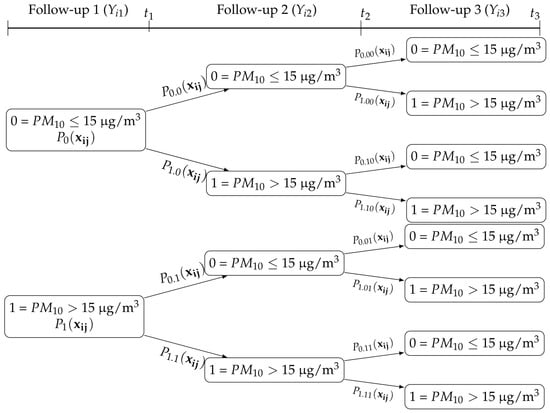
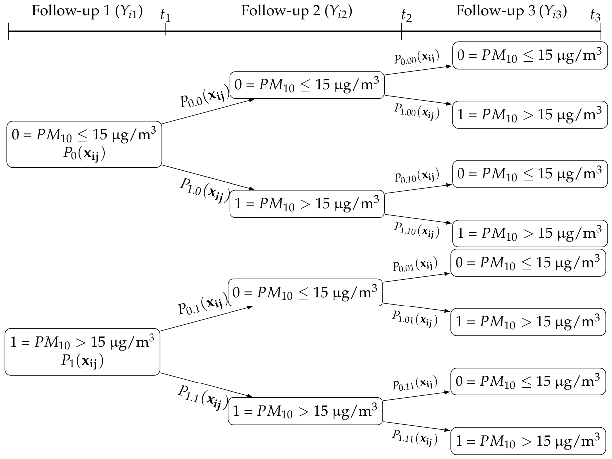
$\mathrm{where}{y}_{ij}=0,1,j=1,\dots ,25$. Equation (3) is also referred to as a first-order Markov chain, where ${\widehat{P}}_{y_1}\left({\mathbf{x}}_{\mathbf{ij}}\right)$ is the marginal probability function of $Y_{i1}$ conditional on the covariate vector ${\mathbf{x}}_{\mathbf{ij}}$ and ${\widehat{P}}_{y_{i2}.y_{i1}}\left({\mathbf{x}}_{i2}\right)$ is the conditional probability function of $Y_{i2}$ conditional on $Y_{i1}$ and ${\mathbf{x}}_{\mathbf{i}\mathbf{2}}$ and so on. In other words, the future outcome depends only on the previous outcome (first-order dependence), but this would require a very large sample size for each time point. The trajectory risk using Equation (3) with three time points shown in Figure 1 would be as follows.

$$\begin{array}{cc}\hfill {\widehat{P}}_{y_{i1},y_{i2},y_{i3}}\left({\mathbf{x}}_{\mathbf{ij}}\right)& =\widehat{P}(Y_{i1}=y_{i1},Y_{i2}=y_{i2},Y_{i3}=y_{i3}\mid {\mathbf{x}}_{\mathbf{ij}})\hfill \\ \hfill & ={\widehat{P}}_{y_{i1}}\left({\mathbf{x}}_{ij}\right)\times {\widehat{P}}_{y_{i2}.y_{i1}}\left({\mathbf{x}}_{ij}\right)\times {\widehat{P}}_{y_{i3}.y_{i2}y}\left({\mathbf{x}}_{\mathbf{ij}}\right).\hfill \end{array}$$

(4)

Figure 1. Transitions of ${PM}_{10}$ states (0, 1) between three follow-up years.

The first column (Follow-up 1), for example, represents the first time point, in our case the year 2000, and $Y_{i1}$ is the outcome variable for this year. The second column (Follow-up 2) represents the second time point, the year 2001, and $Y_{i2}$ is the outcome variable for the second year, and so on. Because our outcomes are binary (0 and 1), we define them in the first column using two boxes with information on how the outcome variable was dichotomized. The model fitted from the first column is the marginal model. We can predict risk for outcome variable categories (e.g., 0 and 1) for different covariate values using the fitted marginal model. In column two, the first two boxes from the top are conditional on the outcome from the first year (2000). So, from the year 2000, those in category 0 can remain in the same category in 2001, or they may change to category 1 in 2001. Using these two groups as the binary outcome, we can fit one conditional model. Similarly, records in 2000 that were in category 1 may remain in the same outcome category in 2001 or change to category 0. Therefore, these two outcomes that moved from category 1 in 2000 allow us to fit the second conditional model for 2001. The interpretation remains the same for the next time points.

3.1. Handling Missing Data

Missing data are inevitable in any longitudinal, time-series, or repeated-measures dataset for various reasons. This is also true for these data; however, they are less prone to error because they are captured automatically via monitors. However, in our proposed modeling framework, data stratification reduces a multivariate problem to a univariate case. Therefore, we can easily apply appropriate missing-data techniques as we would for any cross-sectional dataset. Additionally, outliers do not threaten model building, as the dataset is strictly categorical except for one variable. The proposed framework can also accommodate a varying number of covariates per stratified dataset, which can be handled through additional programming tasks.

3.2. Covariate-Dependent Logistic Regression Models

The logistic regression model is a common choice for studying covariate effects on binary outcomes (transitions) across 51 datasets in Table 5, and the fitted models can be used for risk prediction, accounting for the underlying dependence between consecutive time points [19]. The logistic regression model will model the transition ($Y_{ij}\to Y_{i(j+1)}$) as a function of the covariate vector ${\mathbf{x}}_{ij}$ for the ith site. The first-order conditional probability of $Y_{i2}$ given $Y_{i1}$ and ${\mathbf{x}}_{ij}$ (the probability mass function of $Y_{i2}$ conditional on $Y_{i1}$ and ${\mathbf{x}}_{\mathbf{ij}}$) is expressed as $P(Y_{i2}=y_{i2}\mid Y_{i1}=y_{i1},{\mathbf{x}}_{ij})$ after stratifying the sample based on $Y_{i1}=0$ and $Y_{i1}=1$ as the outcome $Y_{i1}$ is binary. When we stratify the data using $Y_{i1}=0$ and model $Y_{i2}$ as a function of the covariates, we are modeling the transitions from $Y_{i1}=0$ to $Y_{i2}=s$ (i.e., $Y_{i1}=0\to Y_{i2}=s$) where $s=0,1$. Similarly, when we stratify the data using $Y_{i1}=1$ and model $Y_{i2}$ as a function of covariates, we are modeling the transitions ($Y_{i1}=1\to Y_{i2}=s$). In other words, each of these stratified (51) datasets is becoming a univariate dataset; hence, we can use a univariate model. Then the impact of covariates on the first-order conditional model for $P(Y_{i2}=y_{i2}\mid Y_{i1}=0,{\mathbf{x}}_{ij})$ using logistic regression can be shown as:

$$P_{y_{i2}.0}\left({\mathit{x}}_{ij}\right)={\displaystyle \frac{e^{\left({\mathit{x}}_{ij}^{\mathbf{\prime }}{\mathit{\beta }}_{y_2.0}\right)s}}{1+e^{\left({\mathit{x}}_{ij}^{\mathbf{\prime }}{\mathit{\beta }}_{y_2.0}\right)}}},s=0,1,\mathrm{where}{\mathit{\beta }}_{y_2.0}^{\mathbf{\prime }}=\left[{\beta }_{00},{\beta }_{01},\dots ,{\beta }_{0p}\right]$$

(5)

is a $1\times (p+1)$ vector of regression coefficients corresponding to the covariate vector ${\mathbf{x}}_{\mathbf{ij}}^{\mathbf{\prime }}=\left[\mathbf{1},{\mathbf{x}}_{\mathbf{i}\mathbf{1}},\dots ,{\mathbf{x}}_{\mathbf{ip}}\right]$ for the sub-sample stratified on $Y_{i1}=0$. The other first-order conditional model for $P(Y_{i2}=y_{i2}\mid Y_{i1}=1,{\mathbf{x}}_{\mathbf{ij}})$ is:

$$P_{y_{i2}.1}\left({\mathit{x}}_{ij}\right)={\displaystyle \frac{e^{\left({\mathit{x}}_{ij}^{\prime }{\mathit{\beta }}_{{\mathit{y}}_{\mathbf{2}}.\mathbf{1}}\right)s}}{1+e^{\left({\mathit{x}}_{ij}^{\prime }{\mathit{\beta }}_{{\mathit{y}}_{\mathbf{2}}.\mathbf{1}}\right)}}},s=0,1,\mathrm{where}{\mathit{\beta }}_{{\mathit{y}}_{\mathbf{2}}.\mathbf{1}}^{\mathbf{\prime }}=\left[{\beta }_{10},{\beta }_{11},\dots ,{\beta }_{1p}\right]$$

(6)

is a $1\times (p+1)$ vector of regression coefficients corresponding to the covariate vector ${\mathbf{x}}_{\mathbf{ij}}^{\mathbf{\prime }}$ for the sub-sample stratified on $Y_{i1}=1$.

The general form of Equations (5) and (6), $P(Y_{i2}=s\mid Y_{i1}=y_{i1},{\mathbf{x}}_{ij})$, can be shown as:

$$P_{y_{i2}.y_1}\left({\mathit{x}}_{ij}\right)=P(Y_{i2}=s\mid Y_{i1}=y_{i1},{\mathit{x}}_{ij})={\displaystyle \frac{e^{\left({\mathit{x}}_{ij}^{\prime }{\mathit{\beta }}_{{\mathit{y}}_{\mathbf{2}}.{\mathit{y}}_{\mathbf{1}}}\right)s}}{1+e^{\left({\mathit{x}}_{ij}^{\prime }{\mathit{\beta }}_{{\mathit{y}}_{\mathbf{2}}.{\mathit{y}}_{\mathbf{1}}}\right)}}},s,y_1=0,1,$$

(7)

where ${\mathit{\beta }}_{{\mathit{y}}_{\mathbf{2}}.{\mathit{y}}_{\mathbf{1}}}^{\mathbf{\prime }}=\left[{\beta }_{y_{1}0},{\beta }_{y_{1}1},\dots ,{\beta }_{y_{1}p}\right]$ is a $1\times \left[2\right(p+1\left)\right]$ vector of coefficients for the covariate vector ${\mathit{x}}_{ij}^{\mathbf{\prime }}=\left[1,x_1,\dots ,x_p\right]$ for $Y_{i1}=y_{i1}$. This first-order model easily generalizes to higher-order models [17] if the data permit. We can obtain the first-order conditional probabilities for all consecutive outcomes for various values of $\left({\mathit{x}}_{ij}\right)$ using the fitted models in Equation (7). The predicted trajectory risk based on consecutive first-order conditional models can be obtained using the following equation:

$${\widehat{P}}_{y_{i1},y_{i2},\dots ,y_{iJ}}\left({\mathit{x}}_{\mathit{ij}}\right)={\widehat{P}}_{is}\left({\mathit{x}}_{ij}\right)\times {\widehat{P}}_{y_{i2}.y_{i1}}\left({\mathit{x}}_{ij}\right)\times {\widehat{P}}_{y_{i3}.y_{i2}}\left({\mathit{x}}_{ij}\right)\times \dots \times {\widehat{P}}_{y_{ij}.y_{i(j-1)}}\left({\mathit{x}}_{ij}\right).$$

(8)

4. Parameter Estimation

In this section, we discuss the parameter estimation technique for the proposed model. The log-likelihood function of the joint mass function for the first-order Markov chain in (7) can be shown as:

$$\begin{array}{cc}\hfill l& ={\displaystyle \sum _{i=1}^n}{\displaystyle \sum _{j=1}^J}\ln P(Y_{i1}=y_{i1},Y_{i2}=y_{i2},\dots ,Y_{iJ}=y_{iJ}\mid {\mathit{x}}_{\mathit{ij}})={\displaystyle \sum _{i=1}^n}{\displaystyle \sum _{j=1}^J}[\ln P(Y_{i1}=y_{i1}\mid {\mathit{x}}_{\mathit{ij}})\hfill \\ \hfill & +\ln P(Y_{i2}=y_{i2}\mid y_{i1};{\mathit{x}}_{\mathit{ij}})+\dots +\ln P(Y_{iJ}=y_{iJ}\mid y_{i(j-1)};{\mathit{x}}_{\mathit{ij}})]\hfill \\ \hfill & ={\displaystyle \sum _{i=1}^n}{\displaystyle \sum _{j=1}^J}\left[\ln P_{y_1}\left({\mathit{x}}_{\mathit{ij}}\right)+\ln P_{y_2.y_1}\left({\mathit{x}}_{\mathit{ij}}\right)+\dots +\ln P_{y_{iJ}.y_{j-1}}\left({\mathit{x}}_{\mathit{ij}}\right)\right].\hfill \end{array}$$

(9)

Taking the log of the joint mass function converts it into multiple univariate mass functions for each repeated outcome (${\mathbf{Y}}_{ij}$) variable. This shows that each univariate mass function represents a first-order conditional model equal to the marginal model. We can now use logistic regression or any other classification model for a binary outcome for each year. Hence, we can fit all these models in the standard way using an appropriate data structure and Python, R, or other software. We can also use parallel programming to analyze many datasets simultaneously using multiple cores on a single computer or several CPUs in a distributed system.

5. Analysis of ${\mathit{PM}}_{\mathbf{10}}$-Based Air Pollution Data

In this paper, we apply the proposed methodology for analyzing fine particulate matter (${PM}_{10}$)-based air pollution data collected from 1110 sites across various states in the United States. To do that, in Table 7 we first present the list of covariates along with their category descriptions and needed identification variables. We then fit logistic regression models to all 51 stratified datasets. We use a statistical learning approach with leave-one-out cross-validation (LOOCV), a model validation method in which a single data point is used for testing and the remaining data points are used for training, repeating the process for every single point in the dataset. The purpose of this approach is to provide an unbiased estimate of test error and to use almost all data for training at every step, making it well-suited to small datasets. This is appropriate for our analysis, as our datasets are small due to data stratification.

Table 7. Descriptions of covariates used in the models.

Variables	Description	Values
HHIDPN	ID number for each monitor site
EventD ($X_1$)	Occurrence of a wildfire	Yes = 1, No = 0
Elevation ($X_2$)	Measured in meters	Ranges between 0 and 7085
AreaD ($X_3$)	Location of the monitors	Rural = 1, Otherwise = 0
		Rural/Others = 0
LandD ($X_4$)	Type of land utilization	Those that affect $P{M}_{10}$ = 1,
Latitude ($X_5$)	Site Latitude
Longitude ($X_6$)	Site Longitude
DivID	Dataset identification number	1 to 51

5.1. Prediction Accuracy

The model-fitting statistics using LOOCV (e.g., accuracy and Kappa) for all 51 datasets, except dataset 48, are presented in Table 8. For dataset 48, there was no cell frequency for category 1, as shown in Table 5. Out of 51 datasets, 38 had prediction accuracies between 0.80 and 0.99. The prediction accuracies of the remaining 13 datasets range from 0.51 to 0.79.

Table 8. Accuracies of logistic regression models using the LOOCV method for all 51 models.

Datasets	Accuracy	Kappa	ModInfo	Datasets	Accuracy	Kappa	ModInfo
1	0.887	0.166	F1T0M0	27	0.855	−0.014	F1314T11M4
2	0.690	−0.057	F12T01M1	28	0.830	−0.068	F1415T01M3
3	0.980	0.000	F12T11M2	29	0.924	0.000	F1415T11M4
4	0.803	0.364	F23T01M1	30	0.739	0.045	F1516T01M3
5	0.960	0.000	F23T11M2	31	0.952	−0.023	F1516T11M4
6	0.629	−0.099	F34T01M1	32	0.917	0.000	F1617T01M3
7	0.968	0.000	F34T11M2	33	0.835	0.059	F1617T11M4
8	0.756	−0.128	F45T01M1	34	0.761	−0.105	F1718T01M5
9	0.949	0.000	F45T11M2	35	0.902	−0.022	F1718T11M6
10	0.625	−0.131	F56T01M1	36	0.718	−0.092	F1819T01M3
11	0.970	0.000	F56T11M2	37	0.882	−0.043	F1819T11M4
12	0.705	0.159	F67T01M1	38	0.875	−0.049	F1920T01M5
13	0.976	0.000	F67T11M2	39	0.826	−0.051	F1920T11M6
14	0.852	−0.059	F78T01M1	40	0.821	−0.046	F2021T01M3
15	0.976	0.000	F78T11M2	41	0.907	0.000	F2021T11M4
16	0.839	−0.054	F89T01M1	42	0.724	−0.064	F2122T01M5
17	0.962	0.000	F89T11M2	43	0.923	−0.030	F2122T11M6
18	0.912	0.617	F910T01M1	44	0.905	0.000	F2223T01M5
19	0.878	0.000	F910T11M2	45	0.873	−0.066	F2223T11M6
20	0.780	0.553	F1011T01M1	46	0.826	0.233	F2324T01M5
21	0.956	0.551	F1011T11M2	47	0.906	0.236	F2324T11M6
22	0.763	−0.089	F1112T01M1	48	-	-	F2425T01M7
23	0.897	0.000	F1112T11M2	49	0.822	0.234	F2425T11M8
24	0.511	−0.233	F1213T01M3	50	0.760	−0.119	F2526T01M3
25	0.915	−0.012	F1213T11M4	51	0.865	−0.069	F2526T11M4
26	0.886	0.545	F1314T01M3

Note: For dataset 48, category 1 has 0 frequency.

5.2. Trajectory Risk Prediction

To illustrate the trajectory risk, we selected four monitoring sites and predicted their trajectory risks. The IDs for these four sites are (i) 121151006, (ii) 3511013, (iii) 811350, and (iv) 302947. To understand the differences among these four sites, the covariate values for all years are presented in Table 9 and Table 10. We can see that the Area and Land Use values for all of them are the same, whereas Latitude, Longitude, and some event occurrence values differ. The values of the outcome variables (Y) for all years are 1, except for Wave 13 at station 121151006, which is 0.

Table 9. Values of independent variables for two selected sites shown in the figures.

HHIDPN	Wave	Y	Latitude	Longitude	Elevation	Area	Land	Event
3511013	1	1	35.19324	−106.61382	1523	0	1	1
3511013	2	1	35.19324	−106.61382	1523	0	1	1
3511013	3	1	35.19324	−106.61382	1523	0	1	1
3511013	20	1	35.19324	−106.61382	1523	0	1	1
3511013	21	1	35.19324	−106.61382	1523	0	1	1
3511013	22	1	35.19324	−106.61382	1523	0	1	1
3511013	23	1	35.19324	−106.61382	1523	0	1	1
3511013	24	1	35.19324	−106.61382	1523	0	1	1
3511013	25	1	35.19324	−106.61382	1523	0	1	1
3511013	26	1	35.19324	−106.61382	1523	0	1	1
4811350	1	1	32.77426	−96.79769	145	0	1	1
4811350	2	1	32.77426	−96.79769	145	0	1	1
4811350	3	1	32.77426	−96.79769	145	0	1	1
4811350	4	1	32.77426	−96.79769	145	0	1	1
4811350	5	1	32.77426	−96.79769	145	0	1	1
4811350	6	1	32.77426	−96.79769	145	0	1	1
4811350	7	1	32.77426	−96.79769	145	0	1	1
4811350	8	1	32.77426	−96.79769	145	0	1	1
4811350	9	1	32.77426	−96.79769	145	0	1	1
4811350	10	1	32.77426	−96.79769	145	0	1	1
4811350	11	1	32.77426	−96.79769	145	0	1	1
4811350	12	1	32.77426	−96.79769	145	0	1	1
4811350	13	1	32.77426	−96.79769	145	0	1	1
4811350	14	1	32.77426	−96.79769	145	0	1	1
4811350	15	1	32.77426	−96.79769	145	0	1	1
4811350	16	1	32.77426	−96.79769	145	0	1	1
4811350	19	1	32.77426	−96.79769	145	0	1	1
4811350	20	1	32.77426	−96.79769	145	0	1	1
4811350	21	1	32.77426	−96.79769	145	0	1	1
4811350	22	1	32.77426	−96.79769	145	0	1	1
4811350	23	1	32.77426	−96.79769	145	0	1	1
4811350	24	1	32.77426	−96.79769	145	0	1	1
4811350	25	1	32.77426	−96.79769	145	0	1	1
4811350	26	1	32.77426	−96.79769	145	0	1	1

Table 10. Values of independent variables for two selected sites shown in the figures.

HHIDPN	Wave	Y	Latitude	Longitude	Elevation	Area	Land	Event
121151006	1	1	27.35028	−82.47972	11	0	1	1
121151006	2	1	27.35028	−82.47972	11	0	1	1
121151006	4	1	27.35028	−82.47972	11	0	1	1
121151006	5	1	27.35028	−82.47972	11	0	1	1
121151006	6	1	27.35028	−82.47972	11	0	1	1
121151006	7	1	27.35028	−82.47972	11	0	1	1
121151006	8	1	27.35028	−82.47972	11	0	1	1
121151006	9	1	27.35028	−82.47972	11	0	1	1
121151006	10	1	27.35028	−82.47972	11	0	1	1
121151006	11	1	27.35028	−82.47972	11	0	1	1
121151006	12	1	27.35028	−82.47972	11	0	1	1
121151006	13	0	27.35028	−82.47972	11	0	1	1
121151006	14	1	27.35028	−82.47972	11	0	1	1
121151006	15	1	27.35028	−82.47972	11	0	1	1
121151006	16	1	27.35028	−82.47972	11	0	1	1
121151006	17	1	27.35028	−82.47972	11	0	1	1
121151006	18	1	27.35028	−82.47972	11	0	1	1
121151006	19	1	27.35028	−82.47972	11	0	1	1
121151006	20	1	27.35028	−82.47972	11	0	1	1
121151006	21	1	27.35028	−82.47972	11	0	1	1
121151006	22	1	27.35028	−82.47972	11	0	1	1
121151006	23	1	27.35028	−82.47972	11	0	1	1
121151006	24	1	27.35028	−82.47972	11	0	1	1
121151006	25	1	27.35028	−82.47972	11	0	1	1
121151006	26	1	27.35028	−82.47972	11	0	1	1
302947	1	1	48.20054	−114.30533	890	0	1	1
302947	2	1	48.20054	−114.30533	890	0	1	1
302947	3	1	48.20054	−114.30533	890	0	1	1
302947	4	1	48.20054	−114.30533	890	0	1	1
302947	5	1	48.20054	−114.30533	890	0	1	0
302947	6	1	48.20054	−114.30533	890	0	1	0
302947	7	1	48.20054	−114.30533	890	0	1	1
302947	8	1	48.20054	−114.30533	890	0	1	0
302947	9	1	48.20054	−114.30533	890	0	1	1
302947	12	1	48.20054	−114.30533	890	0	1	0
302947	13	1	48.20054	−114.30533	890	0	1	1
302947	14	1	48.20054	−114.30533	890	0	1	1
302947	15	1	48.20054	−114.30533	890	0	1	1
302947	16	1	48.20054	−114.30533	890	0	1	1
302947	17	1	48.20054	−114.30533	890	0	1	1
302947	18	1	48.20054	−114.30533	890	0	1	0
302947	19	1	48.20054	−114.30533	890	0	1	1
302947	20	1	48.20054	−114.30533	890	0	1	1
302947	21	1	48.20054	−114.30533	890	0	1	1
302947	22	1	48.20054	−114.30533	890	0	1	0
302947	23	1	48.20054	−114.30533	890	0	1	1
302947	24	1	48.20054	−114.30533	890	0	1	0
302947	25	1	48.20054	−114.30533	890	0	1	1
302947	26	1	48.20054	−114.30533	890	0	1	1

The predicted conditional probabilities (CP) and the joint probabilities (JP) for these four sites are presented in Table 11. We can see that across all sites, there are some missing values, as is usual for these types of datasets. The predicted conditional probabilities (CP) with values of 0.5 or higher will fall into category 1 for Y, and those less than 0.5 will fall into category 0 for Y, assuming 0.50 as the cutoff threshold. These results help us understand how the fitted models predict risk.

Table 11. Conditional and joint probabilities for four selected sites shown in the figures.

Site ID	3511013		4811350		121151006		302947
Wave (Year)	CP	JP	CP	JP	CP	JP	CP	JP
1	0.96	0.96	0.98	0.98	0.99	0.99	0.80	0.80
2	0.98	0.94	0.99	0.97	0.99	0.98	0.98	0.78
3	0.98	0.92	0.96	0.93			0.95	0.74
4			0.98	0.91			0.90	0.67
5			0.98	0.89	0.98	0.97	1.00	0.67
6			0.97	0.87	0.96	0.93	0.99	0.67
7			0.99	0.86	1.00	0.93	0.95	0.63
8			0.98	0.84	0.98	0.91	1.00	0.63
9			0.99	0.84	0.99	0.90	0.99	0.62
10			0.94	0.79	0.92	0.82
11			0.95	0.75	0.99	0.82
12			0.95	0.72	0.91	0.75
13			0.97	0.69	0.88	0.65	1.00	0.62
14			0.94	0.65	1.00	0.65	0.99	0.62
15			0.97	0.64	0.98	0.64	0.87	0.54
16			1.00	0.63	1.00	0.64	0.99	0.53
17					0.95	0.61	0.94	0.50
18					0.97	0.59	1.00	0.50
19					0.87	0.52	0.96	0.48
20			0.92	0.58	0.92	0.48	0.85	0.40
21	0.99	0.91	0.95	0.56	0.97	0.46	0.86	0.35
22	1.00	0.91	1.00	0.56	1.00	0.46	1.00	0.35
23	1.00	0.91	1.00	0.55	0.99	0.46	1.00	0.35
24	1.00	0.91	1.00	0.55	1.00	0.46	1.00	0.35
25	0.87	0.79	0.97	0.54	0.79	0.36	0.98	0.34
26	1.00	0.79	1.00	0.54	1.00	0.36	1.00	0.34

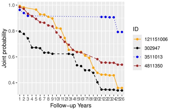
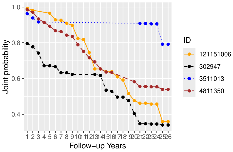
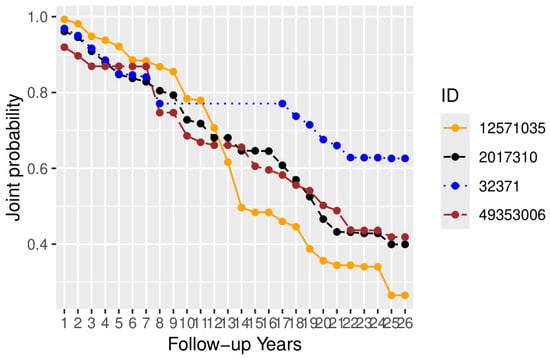
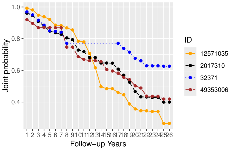
The predicted trajectory risks of joint probabilities for all four stations, shown in Table 11, are presented graphically in Figure 2. We can see that joint probabilities are decreasing gradually, as expected. This is because the joint probabilities are for the full sample in a dataset and are smaller than the conditional probabilities. Conditional probabilities are for the sub-sample, not for the entire dataset. For example, in those datasets, the 51 records that are transitioning from category 1 in the previous year will have higher probabilities than in a dataset conditional on the previous outcome being category 0. In the figure, the trajectory risks for two stations, 121151006 and 4811350, will remain in the high-risk category (joint probabilities are above 0.5 for all the years). However, for the other two stations, these risks have been lower over the last few years, as their joint probabilities are below 0.5. It may be noted that the categories are $1={PM}_{10}$ > 15 μg/m³ and $0={PM}_{10}$ ≤ 15 μg/m³. Similarly, the predicted trajectory risks of joint probabilities for four other stations are presented in Table 11 and Figure 3. We can see a similar trajectory-risk pattern in joint probabilities as in Figure 2.

Figure 2. Model-predicted joint probabilities for four selected stations.

Figure 3. Model-predicted joint probabilities for four different selected stations.

5.3. Comparison of Trajectory Risk Computed from Joint–Marginal and Conditional Model and Independent Models

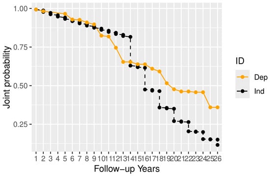
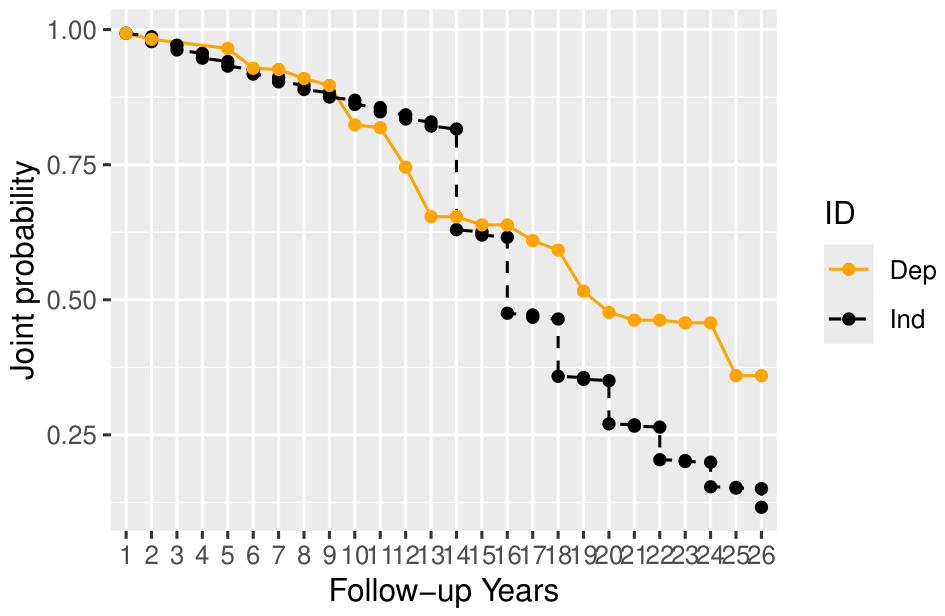
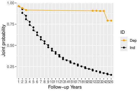
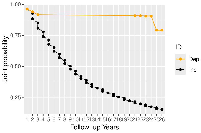
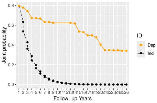
The trajectory risk shown in Figure 2 and Figure 3 is based on the joint model obtained using marginal and conditional models that inherently adjust for temporal dependence. We will now compare the trajectory risk computed using independent models, which do not adjust for temporal dependence. We fitted a logistic regression model to each of the 26 datasets for each year (2000 to 2025), assuming no temporal dependence, and estimated the trajectory risk for station 121151006 using two methods, as shown in Figure 4. Figure 4 shows the trajectory risk for station 121151006 using two methods: Dep (dependent method) with the joint–marginal–conditional approach and Ind (independent method) without any adjustment for temporal dependence. We can see similar trajectory risks for the first 8 years and a wide difference in the later years. In particular, the Ind model is underestimating the trajectory risk. Testing the difference between two lines (trends) over several years involves comparing their slopes (rates of change) and intercepts (starting points) to determine if differences are statistically significant rather than due to sampling error.

Figure 4. Comparison of trajectory risk for station 121151006 using two methods.

To do this, we need to create a new dataset for each station as follows:

• Column 1: Value/Outcome (trajectory risk= joint probabilities);
• Column 2: Wave (Year 1, Year 2, etc., or calendar years like 2020, 2021);
• Column 3: Group—ModelInd (0 for the line from Dep, 1 for the line from IND);
• Column 4: Interaction term: Wave × ModelInd.

Next, we fitted a linear regression and looked at the significance of the estimated coefficient for the interaction term. This coefficient represents the difference between the two lines’ slopes, and we examine the corresponding p-value. If $p<0.01$, the difference between the two trends is statistically significant. If $p\ge 0.05$, we do not have enough evidence to say the trends are different. Table 12 presents the test results using the above regression model for the Dep and Ind models for all four stations. For station 121151006, the interaction term Wave:ModelInd is significant ($p<0.01$). Hence, the difference between the two trends is statistically significant. Figure 5 shows the trajectory risk for station 3511013 using two methods: Dep (dependent method) with the joint–marginal–conditional approach and Ind (independent method) without any adjustment for temporal dependence. We can see a large difference between the two trajectory risks for all years. Also, the regression results for this figure from Table 12 show that the interaction term Wave:ModelInd is significant ($p<0.01$). Hence, the difference between the two trends is statistically significant, and the Ind model substantially underestimates joint probabilities.

Table 12. Testing the difference between two lines over several years.

Term	Estimate	Std. Error	Statistic	p-Value
Model for Site ID: 121151006
Intercept	1.085	0.03	32.95	0.00
Wave	−0.028	0.00	−13.75	0.00
ModelInd	0.094	0.04	2.39	0.02
Wave:ModelInd	−0.012	0.00	−4.90	0.00
Model for Site ID: 3511013
Intercept	0.954	0.04	21.40	0.00
Wave	−0.004	0.00	−1.63	0.11
ModelInd	−0.124	0.05	−2.51	0.02
Wave:ModelInd	−0.027	0.00	−9.80	0.00
Model for Site ID: 811350
Intercept	0.980	0.02	50.56	0.00
Wave	−0.019	0.00	−14.89	0.00
ModelInd	0.109	0.02	4.55	0.00
Wave:ModelInd	−0.022	0.00	−13.68	0.00
Model for Site ID: 302947
Intercept	0.794	0.05	17.48	0.00
Wave	−0.018	0.00	−6.40	0.00
ModelInd	−0.485	0.06	−8.71	0.00
Wave:ModelInd	0.002	0.00	0.57	0.00

Figure 5. Comparison of trajectory risk for station 3511013 using two methods.

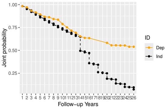
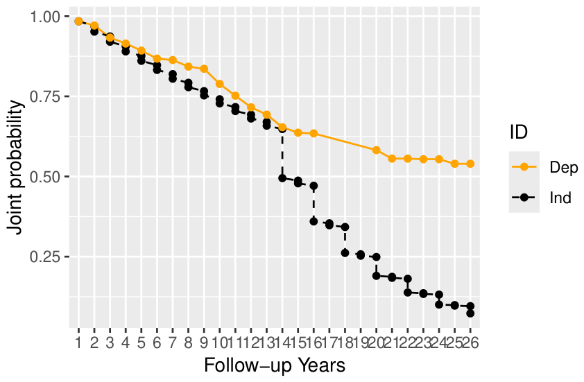
Figure 6 shows the trajectory risk for station 811350 using two methods. A close look at the trajectory risk reveals that the first few years show some difference, and later years show a wide difference. Also, the regression results for this figure from Table 12 show that the interaction term Wave:ModelInd is significant ($p<0.01$). Hence, the difference between the two trends is statistically significant, and the Ind model substantially underestimates joint probabilities.

Figure 6. Comparison of trajectory risk for station 811350 using two methods.

Figure 7 shows the trajectory risk for station 302947 using two methods. A close look at the trajectory risk reveals a wide difference between the two trajectories over the years. Also, the regression results for this figure from Table 12 show that the interaction term Wave:ModelInd is significant ($p<0.01$). Hence, the difference between the two trends is statistically significant, and the Ind model substantially underestimates joint probabilities.

Figure 7. Comparison of trajectory risk for station 302947 using two methods.

6. Discussion

For the analysis of repeated-measures categorical data, particularly those generated from continuous measurements of various environmental variables at monitoring stations, a widely used approach is generalized estimating equations (GEE) for analyzing repeated-measures data using a quasi-likelihood approach with a population-averaged model [28,29]. Because GEE models describe the population-averaged, or marginal, distribution of repeated measurements, they should be used carefully in causal experiments [30]. The authors also concluded that the analysis must generally be conditioned on the previous history of a subject. These environmental data are longitudinal and offer the advantage of visualizing changes in individual responses over time; GEE models cannot achieve this because they describe the population-averaged distribution. In a mixed-effects model, the random component has an unstructured covariance matrix, which could be problematic for this type of data [19]. Conditional models alone are also inadequate for longitudinal data; hence, this paper proposes joint models based on marginal–conditional approaches for analyzing longitudinal data and trajectory risk prediction. We can understand the impact of different covariate values between two stations. For example, in Figure 2, if we compare two stations (121151006 vs. 302947), we can see that the joint probabilities for station 302947 (the first line from the bottom) are lower over the years as compared to those for station 121151006 (the line immediately above station 302947). We can clearly see the impact of elevation on the trajectory risks. For example, the elevation of station 351103 is 1523, much higher than the elevation of 145 for station 4811350; the difference is noticeable. Station 351103, with a much higher elevation, has a very high risk over the years compared to station 4811350. The proposed framework can easily incorporate other machine learning models, e.g., Neural Network, Decision Tree, Support Vector Machine, Naïve Bayes, Random Forest, and many others available for classification. One should replace logistic regression with other machine learning models.

7. Conclusions

We propose a modeling framework to analyze and predict the trajectory risk of repeated binary outcomes using EPA ${PM}_{10}$ air pollution data. These repeated-measures data can be modeled to see how an individual’s outcomes change repeatedly over time [30] and are usually estimated conditional on the subject’s previous outcome. Conditional models are of fundamental interest, and marginal prediction can be derived from them [31]. The proposed framework for trajectory risk prediction uses the relationship between marginal, conditional, and joint probabilities to estimate joint probabilities as the trajectory risk. These joint probabilities are obtained by linking marginal and first-order conditional probabilities from repeated-measures data, i.e., the current-time outcome depends only on the immediately previous outcome. Chowdhury and Islam [19] also predicted joint probabilities for multinomial outcomes by linking marginal and conditional probabilities in a Markov chain. Prediction results from the proposed modeling framework indicate good predictive accuracy for the risk category ${PM}_{10}$ > 15 μg/m³. This is important for policymakers updating guidelines in countries worldwide. More accurate prediction of ${PM}_{10}$ risk categories is critical as it translates complex chemical data into actionable public health warnings, protecting vulnerable populations from severe respiratory and cardiovascular damage [21,32]. In addition, the proposed joint–marginal–conditional framework inherently adjusts risk prediction through data stratification, thereby removing temporal dependence. Section 5.3 illustrates this issue by comparing the proposed model (dependent model) with an independent model that does not account for temporal dependence. Finally, the proposed approach transforms a multivariate problem into a set of univariate problems. The model-fitting process using the proposed framework is mathematically sound. This framework also simplifies trajectory risk prediction and is straightforward and computationally efficient. It is easy, as usual, to include a varying number of covariates at each follow-up, since many new factors may be added in later follow-ups, as in many repeated-measures studies [12]. This model also allows comparison of changes in trajectory risk by changing covariate values of any station, i.e., by creating a new test sample. This would allow policymakers to simulate scenarios by predicting trajectory risks at different levels of risk factors and formulate policies that may help control different types of pollution.

8. Limitations

Our objectives were to develop a modeling framework to analyze ${PM}_{10}$ air pollution data collected through repeated measurements over the years. This type of data is usually messy and complex, with temporal and spatial dependence among repeated outcomes. For this dataset, the sample size declined over the years, which prevents us from fitting other models (e.g., machine learning models). This reduced sample size prevents us from using autologistic regression to adjust for spatial dependence across several stratified datasets. Therefore, we omitted autologistic regression. Various national and international organizations periodically update the danger levels of ${PM}_{10}$. Harmful ${PM}_{10}$ cutoff levels may also vary across age groups. In our proposed framework, we did not use different ${PM}_{10}$ cutoff levels to predict trajectory risk, which is a limitation of the present study. The small sample size over the years also prevented us from doing this. Daily data are available, and using daily ${PM}_{10}$ as dichotomized outcomes may provide enough samples in each category and better risk estimates; this could be investigated in future research. Although interaction terms among covariates in our model can easily be incorporated, we did not do so to keep the length of the paper short. As discussed in the Discussion Section, we did not fit other models to obtain results from this dataset, as our objectives were not to compare our model to others. We omitted presenting the regression coefficient estimates along with other statistics, as this would produce 51 sets of results, multiple tables, and a lengthy paper. We note that the small sample sizes in the stratified sets preclude the use of autologistic regression, limiting the ability to account for spatial dependence. The 15 μg/m³ threshold is also a simplification, and we did not assess sensitivity to it. The reduction in sample sizes over the years may affect both representativeness and trajectory analysis. Also, we did not construct confidence intervals for the predicted probabilities, which could introduce uncertainty when assessing them.

References

- World Health Organization (WHO). Air Pollution. 2026. Available online: https://www.who.int/health-topics/air-pollution#tab=tab_1 (accessed on 10 August 2026).
- World Health Organization (WHO). New SDG Data Shows Stalled Progress on Air Pollution and Health. Departmental Update. Air Pollution. 2026. Available online: https://www.who.int/news/item/29-06-2026-new-sdg-data-shows-stalled-progress-on-air-pollution-and-health (accessed on 10 August 2026).
- Schiavo, B.; Meza-Figueroa, D.; Inguaggiato, C. Environmental Pollution Exposure and Its Human Health Risks. Environments 2026, 13, 421. [Google Scholar] [CrossRef] [Scilit]
- Khadom, A.A.; Albawi, S.; Abboud, A.J.; Mahood, H.B.; Hassan, Q. Predicting air quality index and fine particulate matter levels in Bagdad city using advanced machine learning and deep learning techniques. J. Atmos. Sol.-Terr. Phys. 2024, 262, 106312. [Google Scholar] [CrossRef] [Scilit]
- McDuffie, E.E.; Martin, R.V.; Spadaro, J.V.; Burnett, R.; Smith, S.J.; O’Rourke, P.; Hammer, M.S.; van Donkelaar, A.; Bindle, L.; Shah, V.; et al. Source sector and fuel contributions to ambient PM2.5 and attributable mortality across multiple spatial scales. Nat. Commun. 2021, 12, 3594. [Google Scholar] [CrossRef] [Scilit] [PubMed]
- Landrigan, P.J.; Fuller, R.; Acosta, N.J.R.; Adeyi, O.; Arnold, R.; Basu, N.; Baldé, A.B.; Bertollini, R.; Bose-O’Reilly, S.; Boufford, J.I.; et al. The Lancet Commission on pollution and health. Lancet 2018, 391, 462–512, Erratum in Lancet 2018, 391, 430. [Google Scholar] [CrossRef] [Scilit] [PubMed]
- Prüss-Ustün, A.; Wolf, J.; Corvalán, C.; Neville, T.; Bos, R.; Neira, M. Diseases due to unhealthy environments: An updated estimate of the global burden of disease attributable to environmental determinants of health. J. Public Health 2017, 39, 464–475. [Google Scholar] [CrossRef] [Scilit] [PubMed]
- Thangavel, P.; Park, D.; Lee, Y.C. Recent Insights into Particulate Matter (PM2.5)-Mediated Toxicity in Humans: An Overview. Int. J. Environ. Res. Public Health 2022, 19, 7511. [Google Scholar] [CrossRef] [Scilit] [PubMed]
- Fuge, R. Anthropogenic sources. In Essentials of Medical Geology: Revised Edition; Springer Netherlands: Dordrecht, The Netherlands, 2012; pp. 59–74. [Google Scholar]
- Narges, S.; Majid, F.; Afshin, T.; Parisa, A.; Fatemeh, K.; Mohammad, J.M. Short-term and long-term effects of exposure to PM10. Clin. Epidemiol. Glob. Health 2024, 27, 101611. [Google Scholar] [CrossRef] [Scilit]
- Environmental Protection Agency (EPA), United States. Pre-Generated Data Files. 2020. Available online: https://aqs.epa.gov/aqsweb/airdata//download_files.html (accessed on 10 August 2026).
- Chowdhury, R.; Hasan, M.T. A Modeling Framework Using Markov Chain and Autologistic Regression to Adjust Temporal and Spatial Dependencies for PM2.5 Trajectory Risk Prediction. Environments 2026, 13, 154. [Google Scholar] [CrossRef] [Scilit]
- Ghosh, A.; Maiti, R. Modelling and Forecasting of Complex Multiple Seasonalities in Categorical Time Series Using TSOLR and ISOLR Models. Environmetrics 2026, 37, e70144. [Google Scholar] [CrossRef] [Scilit]
- Rosner, B.; Munoz, A. Autoregressive modeling for the analysis of longitudinal data with unequally spaced examinations. Stat. Med. 1988, 7, 59–71. [Google Scholar] [CrossRef] [Scilit] [PubMed]
- Houria, B.; Abderrahmane, M.; Kenza, K.; Gábor, G. Short-term predictions of PM10 and NO2 concentrations in urban environments based on ARIMA search grid modeling. CLEAN Soil Air Water 2024, 52, 2300395. [Google Scholar] [CrossRef] [Scilit]
- Hossain, M.I.; Sarkar, S.; Methun, M.I.H.; Rahman, A. Exploring regional air pollution transition dynamics: A multi-state markov model approach. PLoS ONE 2025, 20, e0333849. [Google Scholar] [CrossRef] [Scilit] [PubMed]
- Chowdhury, R.I.; Hasan, M.T. Markov regression model for analyzing big data to predict trajectories of repeated categorical outcomes: An application to PM2.5 air pollution data. Environ. Ecol. Stat. 2022, 29, 149–184. [Google Scholar] [CrossRef] [Scilit]
- Hoi, K.I.; Yuen, K.V.; Mok, K.M. Prediction of daily averaged PM10 concentrations by statistical time-varying model. Atmos. Environ. 2009, 43, 2579–2581. [Google Scholar] [CrossRef] [Scilit]
- Islam, M.A.; Chowdhury, R.I. Analysis of Repeated Measures Data; Springer: Singapore, 2017. [Google Scholar]
- Crespo, R.; Manuschevich, D. Using spatial autologistic regression for predicting urban growth. J. Spat. Sci. 2023, 68, 651–666. [Google Scholar] [CrossRef] [Scilit]
- PM10 (Coarse Particulate Matter): Sources, Health Effects & Dust Monitoring. Air Quality Measurement Series. 2026. Available online: https://www.clarity.io/blog/air-quality-measurement-series-dust-pm10 (accessed on 1 August 2026).
- World Health Organization. WHO Global Air Quality Guidelines: Particulate Matter (PM2.5 and PM10), Ozone, Nitrogen Dioxide, Sulfur Dioxide and Carbon Monoxide; World Health Organization: Geneva, Switzerland, 2021; Available online: https://www.who.int/publications/i/item/9789240034228 (accessed on 19 September 2026).
- What Is PM2.5 and PM10? Info About Particulate Matter (Particle Pollution). Available online: https://airly.org/en/what-is-pm10-and-what-is-pm2-5/ (accessed on 19 September 2026).
- Air Pollution. A Major Public Health Issue. Air Pollution Is Now Recognized as the Greatest Environmental Threat to Human Health. WHO Global Air Quality Guidelines. 2021. Available online: https://www.parapm.org/en/air-pollution/ (accessed on 19 September 2026).
- The Contents of the Pre-Generated Files and Variable Descriptions. AirData Download Files Documentation: Version 3.0.0. 2015. Available online: https://aqs.epa.gov/aqsweb/airdata/FileFormats.html (accessed on 19 September 2025).
- AirData: Air Quality Data Collected at Outdoor Monitors Across the US. 2026. Available online: https://www.epa.gov/outdoor-air-quality-data (accessed on 19 September 2026).
- Moran, P. The interpolation of statistical maps. J. R. Stat. Soc. Ser. B Stat. Methodol. 1948, 10, 243–251. [Google Scholar] [CrossRef] [Scilit]
- Liang, K.Y.; Zeger, S.L. Longitudinal data analysis using generalized linear models. Biometrika 1986, 73, 13–22. [Google Scholar] [CrossRef]
- Zeger, S.L.; Liang, K.Y. Longitudinal data analysis for discrete and continuous outcomes. Biometrics 1986, 42, 121–130. [Google Scholar] [CrossRef] [Scilit]
- Lindsey, J.K.; Lambert, P. On the appropriateness of marginal models for repeated measurements in clinical trials. Stat. Med. 1998, 17, 447–469. [Google Scholar] [CrossRef]
- Lee, Y.; Nelder, J.A. Conditional and Marginal Models: Another View. Stat. Sci. 2004, 19, 219–238. [Google Scholar] [CrossRef] [Scilit]
- Krismanuel, H. Air pollution and cardiovascular diseases: Mechanisms, evidence, and mitigation strategies. J. Med. Life 2025, 18, 411–427. [Google Scholar] [CrossRef] [Scilit] [PubMed]
Disclaimer/Publisher’s Note: The statements, opinions and data contained in all publications are solely those of the individual author(s) and contributor(s) and not of MDPI and/or the editor(s). MDPI and/or the editor(s) disclaim responsibility for any injury to people or property resulting from any ideas, methods, instructions or products referred to in the content. |
© 2026 by the authors. Licensee MDPI, Basel, Switzerland. This article is an open access article distributed under the terms and conditions of the Creative Commons Attribution (CC BY) license.