Exploring the Interaction of Transit Accessibility, Housing Affordability, and Low-Income Household Displacement: A Statistical and Spatial Analysis of Tennessee Counties

Abstract

Urban sustainability depends on balancing transportation accessibility, housing affordability, and social equity. Displacement—defined in this study as the population-level loss of low-income households from a census block over time—poses a growing challenge to inclusive urban development. This study examines statistical relationships and spatial patterns linking transit accessibility, housing affordability, and low-income household displacement across the four largest counties in Tennessee. Negative binomial regression models are used to quantify relationships between transit accessibility, housing affordability, and displacement, revealing that housing affordability is consistently linked to displacement, while the effects of transit accessibility vary substantially across counties. Bivariate Local Indicators of Spatial Association (LISA) identify localized clusters where displacement coincides with transit or housing constraints, and Multivariate Cluster Typology Analysis classifies census blocks into distinct typologies, highlighting region-specific trade-offs between accessibility and affordability. Together, the results demonstrate that displacement dynamics are highly context dependent, underscoring the need for place-based and sustainability-oriented policy responses. The findings provide an empirical basis for integrating transportation and housing strategies to reduce displacement risks and support equitable and sustainable urban development in diverse metropolitan contexts.

1. Introduction

Urban displacement, a significant consequence of gentrification, has garnered increasing attention due to its implications for social equity and urban planning [1]. Over the last decade, metropolitan regions across the United States, including major counties in Tennessee, have witnessed rising housing costs and demographic shifts, particularly in city centers. While these changes often signal economic revitalization, they disproportionately affect vulnerable populations, especially low-income households. These households are frequently forced to relocate to suburban or exurban areas where housing is more affordable. However, transit systems, designed to serve dense urban cores, often provide less frequent and less connected services in suburban and exurban areas, creating significant barriers to mobility and access to opportunities for displaced low-income households. This mismatch between housing affordability and transit accessibility underscores the urgency of addressing transportation and housing challenges in tandem. Strategic interventions, such as expanding affordable housing near transit-rich areas or improving transit networks in low-cost housing zones, are essential for promoting equitable urban development. However, such efforts require a nuanced understanding of the spatial and statistical dynamics that drive displacement and its associated challenges.

Previous studies have examined displacement, transit accessibility, and housing affordability using either non-spatial statistical models or spatial analytical techniques, but rarely in an integrated manner. Regression-based approaches are effective for estimating average relationships while controlling for confounding factors, yet they typically assume spatial independence and provide limited insight into local spatial heterogeneity [2,3]. Conversely, spatial methods such as cluster analysis or Local Indicators of Spatial Association (LISA) reveal geographic concentrations and local autocorrelation but do not quantify the simultaneous influence of multiple explanatory variables [4,5,6]. As a result, existing research often provides either explanatory insight or spatial characterization, but not both within a unified framework. This methodological separation constrains the development of evidence that is simultaneously statistically robust and geographically actionable. Furthermore, while transit accessibility is a primary focus in prior studies, it is increasingly recognized that infrastructure utilization is heavily mediated by the factors influencing an individual’s mode choice. Previous research, such as the application of logit models in the Górnośląska-Zagłębiowska Metropolis, has demonstrated that sociodemographic characteristics—including education levels and economic status—fundamentally shape the decision to utilize public transportation for daily travel activities [7]. Consequently, displacement research may look beyond physical proximity to transit and account for the sociodemographic drivers of realized transit usage, as these factors collectively determine a household’s interaction with the urban environment and their vulnerability to rising housing pressures.

This study addresses these limitations by employing a comprehensive framework that integrates statistical modeling and spatial analysis techniques. Using publicly available datasets and open-source tools, this research analyzes displacement dynamics across Davidson (containing the City of Nashville), Shelby (containing the City of Memphis), Knox (containing the City of Knoxville), and Hamilton (containing the City of Chattanooga) counties in Tennessee. Statistical analysis employs negative binomial regression to quantify the effects of transit accessibility and housing affordability on low-income household displacement, while explicitly controlling for the sociodemographic and demographic factors that influence both transit dependency and residential stability. The spatial analysis combines Bivariate Local Indicators of Spatial Association (LISA) to identify localized correlations and Multivariate Cluster Typology Analysis to classify regions based on displacement patterns, transit accessibility, and housing affordability. The integration of statistical and spatial analyses provides a more comprehensive perspective by jointly capturing explanatory relationships and spatial heterogeneity. By combining regression-based inference with spatial pattern identification, this approach addresses limitations inherent in studies that rely exclusively on either statistical or spatial methods. Tennessee provides a particularly informative and representative context for this analysis. Its major metropolitan counties have experienced uneven urban growth, redevelopment, and demographic change, while operating relatively constrained public transit systems compared to larger U.S. metropolitan regions. This combination of rapid housing market shifts, persistent income inequality, and limited transit provision creates conditions in which displacement risks are both pronounced and spatially heterogeneous, making Tennessee counties a suitable case for examining how transit accessibility and housing affordability interact to shape displacement dynamics in medium-sized metropolitan areas.

This study makes several key contributions to the field. First, it bridges the gap between statistical and spatial analyses, offering a more nuanced understanding of the factors driving low-income household displacement. Second, it provides a scalable methodology that leverages publicly available datasets and open-source tools (e.g., Conveyal’s Analysis tool), making it applicable to diverse urban contexts. Third, the research highlights actionable policy implications, such as identifying priority areas for housing and transit improvements, to promote equitable urban development.

The remainder of this paper is structured as follows. Section 2 reviews the literature on displacement, transit accessibility, and housing affordability. Section 3 introduces the datasets and variable constructions. Section 4 details the statistical and spatial modeling methodologies. Section 5 presents the results and discusses their implications for policy and practice. Finally, Section 6 concludes the study and offers recommendations for future research.

2. Literature Review

This section reviews prior studies in three parts. First, studies on the displacement of low-income households are summarized. Next, research on transit accessibility is discussed. Finally, studies exploring the interaction between these factors are highlighted, along with their methodological approaches and limitations.

2.1. Displacement of Low-Income Households

Displacement is a central concern of gentrification [8], and measuring residential displacement has long posed methodological challenges [9]. Some studies identify displacement through involuntary residential moves, explicitly distinguishing moves driven by external pressures from voluntary relocation [10,11,12,13]. A summary of common displacement measurements used in prior studies is provided in

Table 1. Summary of displacement measurements in prior studies.

Approach	Core Concept	Typical Data Sources	Strengths	Limitations
Motivational approach	Identifies displacement based on involuntary reasons for residential moves	Household surveys, interviews	Directly captures displacement intent and experience	Data-intensive; limited spatial and temporal coverage
Individual approach	Tracks individual or household mobility over time regardless of motivation	Longitudinal administrative or panel data	Enables causal and temporal analysis of mobility	Limited availability; often lacks spatial detail
Population approach	Infers displacement from changes in the concentration or loss of low-income households	Census and ACS data	Scalable; spatially explicit; suitable for regional analysis	Does not directly observe individual displacement events

. The “motivational approach” focuses on the reasons for mobility but relies heavily on detailed survey or administrative data [10]. In contrast, the “individual approach” traces individual longitudinal residential mobility at the household or individual level without distinguishing the underlying motivations for moving [14,15]. However, the extensive data requirements of both approaches often limit their applicability, particularly for large-scale spatial analyses. To address these constraints, the University of California, Berkeley’s Urban Displacement Project (UDP) proposed a “population approach” that measures displacement using publicly available census data, focusing on the loss of low-income households over time [16]. This approach is well suited for identifying spatial patterns of displacement risk and comparing trends across regions [17]. Accordingly, the population approach is adopted in this study. While population-based measures have been widely applied, limited attention has been paid to the spatial clustering of displacement and its interaction with other spatially structured factors, such as transit accessibility and housing affordability. To address this gap, this study incorporates spatial analysis techniques, including Bivariate LISA, to examine how displacement patterns intersect with these urban characteristics.

2.2. Transit Accessibility

The transportation literature increasingly emphasizes accessibility—defined as the ability to reach opportunities—over mobility, which focuses on the efficient movement of people and goods. Recent studies have explored transit accessibility by analyzing the geographic area and number of opportunities, such as jobs, that one can reach within a given time threshold using transit [18,19,20,21]. Transit accessibility is often calculated using digital transit schedule datasets in the General Transit Feed Specification (GTFS) format provided by transit agencies [22]. A range of software tools has been developed to operationalize transit accessibility analysis. Established proprietary platforms such as ArcGIS and Emme offer robust network analysis capabilities but often require costly licenses and extensive manual preprocessing, limiting reproducibility and scalability across regions. Open-source alternatives, including OpenTripPlanner Analyst and the r5r package in R, enable detailed accessibility calculations using the Rapid Realistic Routing (R5) engine and have been widely adopted in research settings [23]. However, these tools generally require programming expertise and additional effort to integrate transit networks with large-scale employment datasets.

For this study, Conveyal Analysis was selected because it offers several advantages over both proprietary GIS platforms and programming-intensive open-source tools [24]. First, Conveyal provides native integration of GTFS transit networks with the Longitudinal Employer-Household Dynamics (LEHD) Origin-Destination Employment Statistics (LODES) dataset, enabling efficient, consistent computation of job accessibility without additional data harmonization. Second, its web-based interface supports large-scale, reproducible accessibility analysis across multiple counties, while maintaining methodological transparency. Third, Conveyal uses the same R5 routing engine as r5r but removes the need for custom scripting, reducing implementation complexity while preserving analytical rigor. Conveyal Analysis was accessed via a web browser using the open-source version of the platform (MIT license). All accessibility calculations were performed online using publicly available GTFS and LODES datasets. Community documentation and user forums provided by the Conveyal development team were consulted to support implementation and validation of the analysis workflow. This combination of open-source licensing, web-based accessibility modeling, and interoperability with national-scale employment data offers a practical and reproducible approach for transit accessibility research across diverse geographic contexts.

2.3. Housing Affordability

Housing affordability is a fundamental determinant of residential stability, representing the relationship between household income and housing expenditures. At its most fundamental level, affordability reflects the challenge households face in balancing housing costs against essential non-housing needs [25]. While this balance is influenced by economic policies and market supply [26], researchers typically evaluate this relationship through the “ratio paradigm,” which measures the proportion of income spent on housing. The 30% income-to-cost threshold is the most common standard used to identify households at risk of housing instability [16,27]. However, traditional applications of this ratio often provide a broad estimate of cost burden without distinguishing between different levels of market affordability at the neighborhood scale. As noted in previous research, aggregate metrics often fail to reveal how affordable housing stock is distributed across different socio-economic groups or sub-markets [28]. This study addresses these limitations by transitioning from individual cost-burden analysis to a multi-tier spatial classification of market affordability. Our approach categorizes housing stock into distinct low-, moderate-, and high-cost tiers based on regional income thresholds. By aggregating these unit-level data into census tract typologies, this method identifies the predominant affordability profile of a specific area. This framework allows for a more detailed analysis of how different levels of housing cost contribute to low-income displacement, bridging the gap between individual financial constraints and neighborhood-scale market trends.

2.4. Transit Accessibility, Housing Affordability, and the Displacement of Low-Income Households

Previous studies exploring the relationship between transit accessibility and the spatial distribution of low-income households have reported differing findings, reflecting strong contextual dependence rather than a single definitive pattern. Some studies find that bus routes are more prevalent in low-income neighborhoods, consistent with higher transit reliance among these households [29,30,31]. Others show that areas with well-developed transit networks are associated with higher housing prices and greater attraction of higher-income residents [32,33]. A third group finds that transit development can increase housing values over time, contributing to the displacement of low-income households [34,35]. These differing findings indicate that the impacts of transit accessibility and housing affordability on low-income households are highly context-dependent and do not follow a uniform pattern across regions. These variations can be attributed to differences in regional housing market dynamics, transit system characteristics, and methodological choices across studies.

While prior studies have established important associations between transit and housing outcomes, they have often relied on aggregate or global analytical approaches that may obscure localized spatial heterogeneities. To address this limitation, this study incorporates advanced spatial analyses to examine displacement patterns at a finer geographic scale. Specifically, Bivariate LISA is used to identify localized clusters of concern—regions where displacement overlaps with transit or housing challenges. This approach enables the detection of place-specific spatial associations that are not captured by global models. Building on this, Multivariate Cluster Typology Analysis is applied to classify regions into distinct typologies, reflecting the combined spatial characteristics of transit accessibility, housing affordability, and displacement. By integrating these spatial techniques, this study enhances existing approaches and provides a more nuanced understanding of displacement dynamics across neighborhoods.

2.5. Summary of Research Gaps

In summary, the existing literature demonstrates that the relationship between transit accessibility, housing affordability, and displacement is highly context-dependent, with findings often varying across different urban environments. While the “population approach” has become a practical standard for measuring displacement risk and advanced tools allow for precise accessibility modeling, a significant methodological gap persists in the integration of these dimensions.

Current research remains largely divided between statistical techniques that identify general regional relationships and spatial methods that visualize geographic patterns. The former often overlooks localized spatial heterogeneities, while the latter lacks the analytical depth provided by multivariate modeling. This study addresses these limitations by integrating negative binomial regression with Bivariate LISA and Multivariate Cluster Typology. This integrated framework bridges the gap between explanatory modeling and spatial pattern recognition, providing a more comprehensive and spatially nuanced understanding of the diverse factors driving displacement at the neighborhood scale.

3. Study Area and Data

This section introduces the study area, outlines the data sources, and describes the key variables used in the analysis. All data were collected prior to the COVID-19 pandemic.

3.1. Study Area

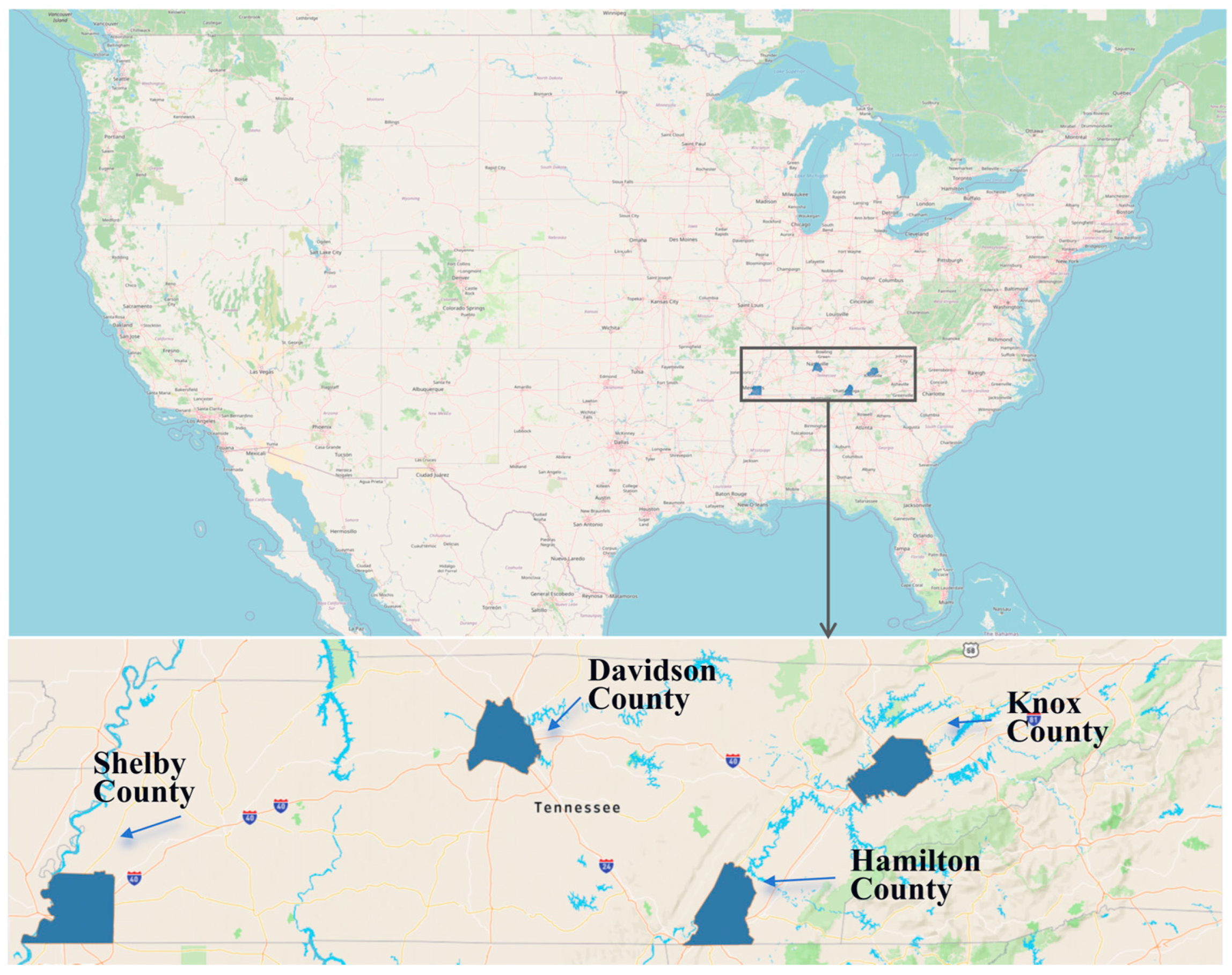
This study focuses on four major metropolitan counties in Tennessee: Davidson, Shelby, Knox, and Hamilton. These counties represent distinct demographic, housing, and transportation contexts that together provide a comprehensive basis for examining the interplay between displacement, transit accessibility, and housing affordability. Their locations within the state are shown in Figure 1.

Davidson County, containing the state capital of Nashville, has undergone rapid population growth and redevelopment, generating substantial pressures on housing affordability. Rising housing costs and neighborhood change have heightened displacement risks for low-income households [36]. Public transit is provided by WeGo Public Transit through a bus network and a limited commuter rail line, though overall coverage remains constrained relative to demand. Shelby County, containing Memphis, is the state’s most populous county and faces persistent socioeconomic challenges. Median household incomes remain below the national average, and poverty rates are among the highest among large U.S. metropolitan areas. These conditions contribute to widespread housing cost burdens. The Memphis Area Transit Authority (MATA) operates bus and trolley services, but coverage and service frequency are limited, providing only modest regional mobility. Knox County, containing Knoxville, presents an intermediate case. Revitalization efforts in the downtown core have spurred redevelopment, increasing property values and producing localized affordability pressures [37]. Knoxville Area Transit (KAT) operates the public transit system, yet automobile dependence remains high, and affordable housing near revitalized areas has become increasingly scarce. Hamilton County, containing Chattanooga, has traditionally been considered more affordable, but recent growth pressures have significantly eroded housing affordability. Rising rents, a declining supply of affordable housing, and growing barriers to home ownership have intensified cost burdens, particularly for low-income households. Transit services, provided by the Chattanooga Area Regional Transportation Authority (CARTA), are limited, leaving vulnerable populations especially exposed where affordability pressures intersect with constrained mobility options.

Taken together, these four counties span a spectrum of urban development and socioeconomic conditions—from rapidly gentrifying regions to persistently low-income communities and areas of emerging affordability stress. This diversity makes them a representative and analytically valuable setting for assessing how displacement patterns among low-income households intersect with transit accessibility and housing affordability.

3.2. Data Sources

3.2.1. Socioeconomic Information

Socioeconomic data were obtained from the U.S. Census Bureau at the tract level. To analyze the displacement of low-income households from 2010 to 2019, data from the 2006–2010 and 2014–2019 American Community Survey (ACS) were used. These datasets provide detailed information on population characteristics, income, and housing costs. In addition to income- and housing-related information, the analysis incorporated three socioeconomic characteristics related to education, ethnicity, and travel behavior to control for broader determinants of residential stability. The educational attainment measure was selected to serve as a proxy for workforce competitiveness and household economic resilience, which distinctively influence displacement risks. Concurrently, the variable representing ethnic composition was included to control for unobserved structural disparities and differential access within the housing market. Finally, data on transit commuting was utilized to capture realized system reliance, thereby distinguishing actual user demand from the theoretical network accessibility modeled in subsequent sections.

3.2.2. Employment Opportunities Information

Employment data were sourced from the Longitudinal Employer-Household Dynamics (LEHD) Origin-Destination Employment Statistics (LODES) dataset, which offers detailed information on home and work locations of employed individuals at the census block level. The analysis used the “JT00” (All Jobs) category, which represents formal sector employment, including jobs covered by state employment insurance systems and most federal government positions. This dataset was utilized to determine the geographic distribution of jobs in 2019, essential for calculating transit accessibility.

3.2.3. Transit Information

Transit schedules and networks were obtained using the General Transit Feed Specification (GTFS), a standardized format widely used in transit accessibility research. The 2019 GTFS data for the primary transit agencies in each of Tennessee’s four largest counties were employed to simulate transit travel times during weekday morning peak hours (7–10 a.m.) using Conveyal’s analysis tool. The GTFS datasets were validated for completeness, schedule consistency, and stop accuracy prior to analysis. Any missing or inconsistent entries were corrected using official agency updates and cross-referenced with transit maps.

3.2.4. Geographic Layer

Geographic layers, including the census tract and block layers from the 2010 U.S. Census Bureau, were used to spatially align socioeconomic and transit data. Census block layers, offering finer spatial resolution, were used for transit accessibility calculations, while census tract layers were applied to analyze socioeconomic variables. Each census block inherited the socioeconomic attributes of its corresponding census tract.

3.3. Explanatory Variables

3.3.1. Transit Accessibility Variable Construction

Transit accessibility was measured as the number of jobs accessible by transit within a 90 min threshold during weekday morning peak hours. While prior studies often adopt a 60 min cutoff when assessing transit accessibility in metropolitan contexts [38,39,40,41], this study encompasses both urban centers and suburban/peripheral areas across four counties in Tennessee, where transit trips to major employment centers frequently exceed one hour. Given the focus on displacement of low-income households, it was necessary to consider longer commutes that more accurately reflect the conditions faced by households relocating to suburban or outskirt areas. Adopting a 90 min threshold therefore provides a more comprehensive and inclusive measure of accessibility in the context of our study. Using Conveyal’s Analysis tool, job locations from the 2019 LODES dataset and transit schedules from the 2019 GTFS data were combined. The centroid of each census block was used as the origin for accessibility calculations, capturing spatial variations across the study area.

3.3.2. Low-Income Households and Loss of Low-Income Households

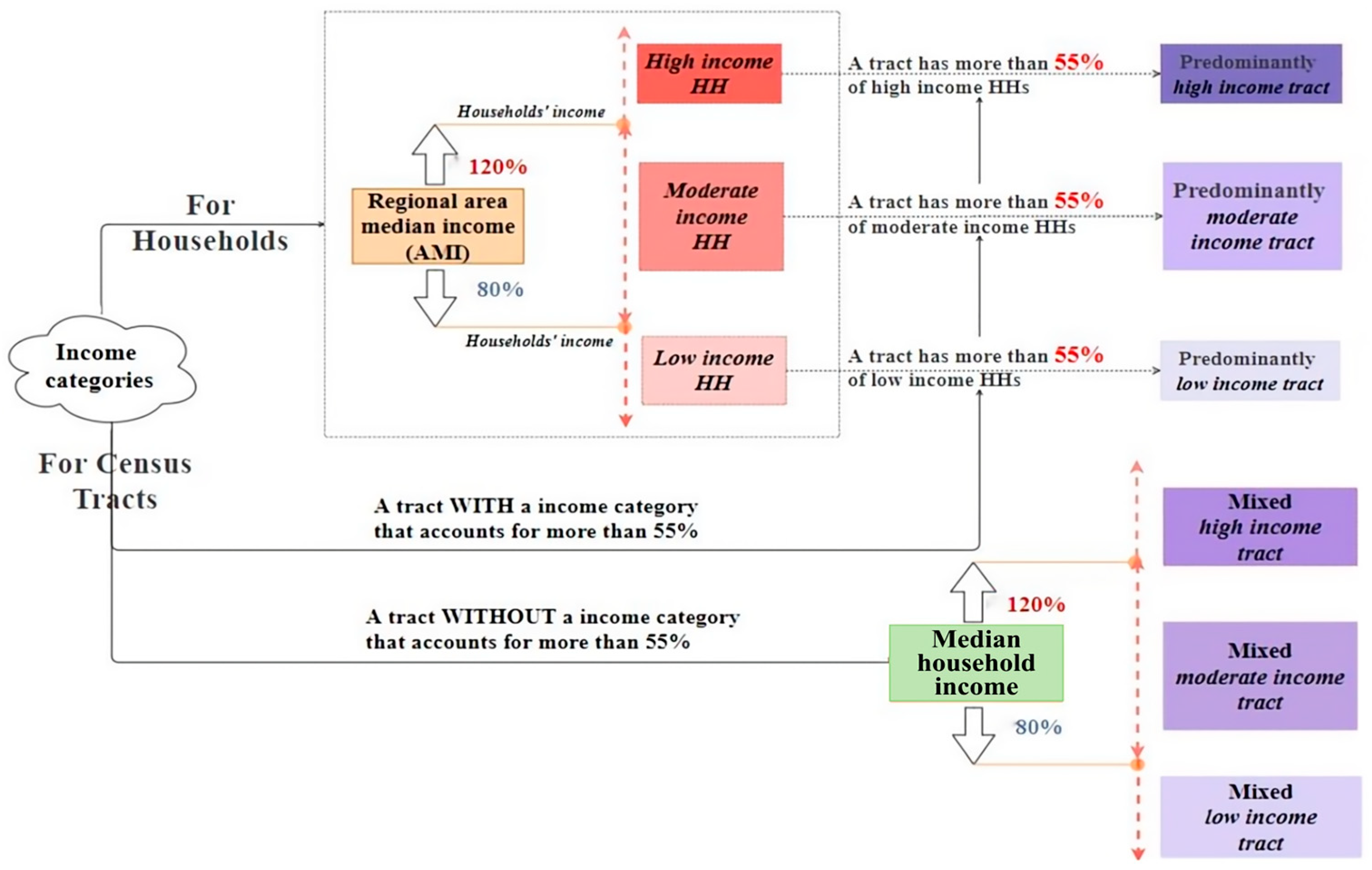
The number of low-income households was estimated using ACS data, which reports household counts across income intervals. Income categories were aggregated according to the Urban Displacement Project (UDP) definition, where households earning less than 80% of the regional area median income (AMI) are classified as low-income (as illustrated in Figure 2) [16]. Displacement was calculated as the change in the number of low-income households in each census tract from 2010 to 2019.

3.3.3. Income Category

To categorize census tracts by income levels, this study followed the classification framework developed by the Urban Displacement Project [16]. In this framework, households earning less than 80% of the area median income (AMI) are classified as low-income, those earning between 80% and 120% of AMI are classified as moderate-income, and those earning above 120% of AMI are classified as high-income. Based on the proportion of households at different income levels, tracts were classified into six categories. Figure 2 illustrates the process of identifying income categories.

3.3.4. Low-Cost Housing and Housing Affordability

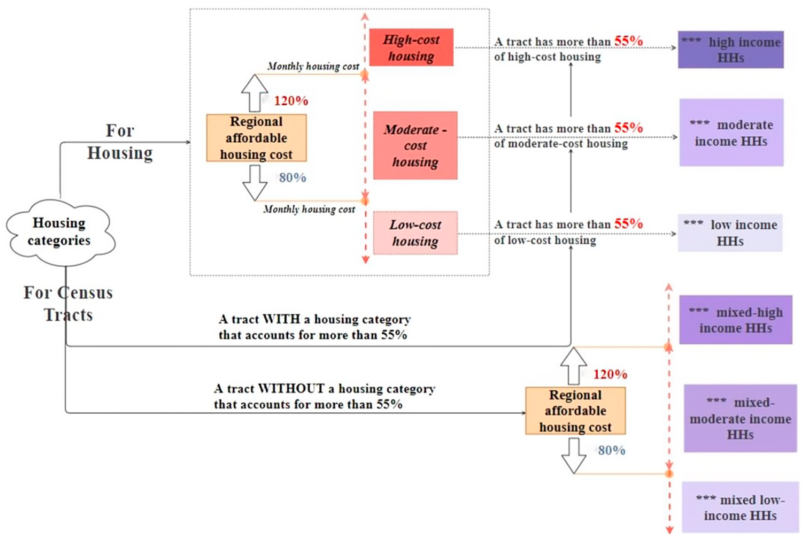
“Housing costs” were measured using the ACS Selected Monthly Owner Costs variable, which includes mortgage payments, home equity loans, real estate taxes, homeowner’s insurance, utilities, fuels, and condominium or association fees. This variable captures the full financial cost of home ownership, providing an indicator of overall market affordability at the neighborhood scale. Housing affordability was evaluated by comparing housing costs to income levels, based on the assumption that housing is affordable when it costs less than 30% of a household’s monthly income [16]. Figure 3 illustrates the steps for identifying housing affordability categories at the census tract level. Following established practice, the analysis proceeded in two steps:

(1)

Housing unit-level cost categorization:

Housing units were classified into three cost levels based on their relationship to the regional affordable housing threshold:

• Low-Cost Housing: Monthly costs below 80% of the regional affordable housing threshold.
• Moderate-Cost Housing: Monthly costs between 80% and 120% of the regional affordable housing threshold.
• High-Cost Housing: Monthly costs above 120% of the regional affordable housing threshold.

(2)

Census tract-level affordability classification:

Using the above cost categories, census tracts were grouped into six affordability types:

• Housing Affordable to Low-Income Households: 55% or more low-cost housing.
• Housing Affordable to Moderate-Income Households: 55% or more moderate-cost housing.
• Housing Affordable to High-Income Households: 55% or more high-cost housing.
• Housing Affordable to Mixed Low-Income Households: Tracts without predominant affordability but with a median housing cost below 80% of the regional affordable housing threshold.
• Housing Affordable to Mixed Moderate-Income Households: Tracts without predominant affordability but with a median housing cost between 80% and 120% of the regional affordable housing threshold.
• Housing Affordable to Mixed High-Income Households: Tracts without predominant affordability but with a median housing cost above 120% of the regional affordable housing threshold.

4. Method

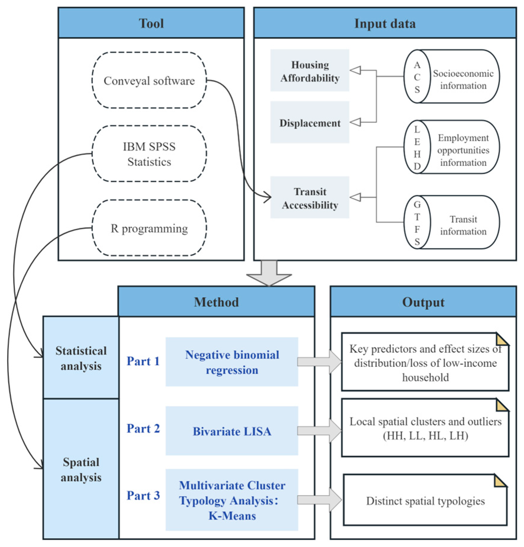
This analysis integrates statistical modeling and spatial analysis to investigate how transit accessibility and housing affordability relate to the spatial distribution and displacement of low-income households across Tennessee’s four largest counties between 2010 and 2019. To achieve this objective, a three-part methodological framework was adopted, as illustrated in Figure 4. First, descriptive statistics and spatial visualizations were used to analyze income categories, housing affordability, and displacement patterns, providing an initial understanding of spatial correlations. Second, negative binomial regression models were conducted in IBM SPSS Statistics (version 27) to quantify the effects of transit accessibility and housing affordability on the distribution and loss of low-income households. Third, spatial analyses using Bivariate LISA identified significant spatial clusters, while Multivariate Cluster Typology Analysis (K-means) categorized areas into typologies based on transit accessibility, housing affordability, and displacement characteristics, revealing distinct spatial patterns.

4.1. Statistical Modeling Approach

This study utilized two response variables: the number of low-income households in 2019 and the loss of low-income households from 2010 to 2019. Since both response variables are non-negative integers, count models were deemed appropriate. A comparison of the observed variance and mean for each variable revealed overdispersion in the data. Consequently, negative binomial regression models were employed, as they are better suited for handling overdispersed data compared to Poisson models [42,43]. Adopting the standard formulation found in established econometric literature [43], the negative binomial regression framework is expressed in Equations (1)–(3) below as follows:

$$P \left({Y=y}_i\right)= {\displaystyle \frac{\mathsf{\Gamma }({\mathsf{\alpha }}^{-1}+y_i)}{\mathsf{\Gamma }(y_i+1)\ast \mathsf{\Gamma }({\mathsf{\alpha }}^{-1})}}\ast ({{\displaystyle \frac{1}{1+\mathsf{\alpha }{\lambda }_i}})}^{{\mathsf{\alpha }}^{-1}}\ast {({\displaystyle \frac{\mathsf{\alpha }{\lambda }_i}{1+\mathsf{\alpha }{\lambda }_i}})}^{y_i}$$

(1)

$${\lambda }_i=\exp \left(\beta X_i+{ϵ}_i\right)$$

(2)

$$var\left(y_i\right)=E\left(y_i\right)\ast [1+\alpha \ast E(y_i\left)\right]$$

(3)

where

• $y_i$ = the response value of the $i^{\mathrm{t}\mathrm{h}}$ observation (i.e., the number of low-income households in 2019 or the loss of low-income households from 2010 to 2019 in the census tract to which the $i^{\mathrm{t}\mathrm{h}}$ census block belongs);
• $P\left({Y=y}_i\right)$ = the probability of the response value of the $i^{\mathrm{t}\mathrm{h}}$ observation;
• $\mathsf{\Gamma }(.)$ = the value of the gamma distribution;
• ${\lambda }_i=$ the expected response value of the $i^{\mathrm{t}\mathrm{h}}$ observation;
• $X_i$ = a vector of explanatory variables (e.g., the number of low-cost housing units in the census tract to which the $i^{\mathrm{t}\mathrm{h}}$ census block belongs);
• $\beta$ = a vector of coefficients that are estimated;
• $ϵ$ = an independently distributed error term into the equation of ${\lambda }_i$ to prevent over-dispersion caused by the difference in the mean and variance of the response variable;
• $\alpha$ = a dispersion parameter that is used to measure the dispersion of a model. When $\alpha$ is equal to 0, then the negative binomial model works like the Poisson model.

4.2. Spatial Modeling Approach

This section employs spatial analysis methods to investigate the interplay between transit accessibility, housing affordability, and low-income household displacement. The primary objectives are to identify spatial clusters and typologies that highlight areas with pronounced displacement patterns and their relationship with varying levels of transit accessibility and housing affordability. The approach integrates two key methods: Bivariate LISA and Multivariate Cluster Typology Analysis, providing a nuanced understanding of spatial patterns and disparities. Bivariate LISA examines localized spatial relationships between pairs of variables, such as displacement and transit accessibility or displacement and housing affordability. This analysis identifies clusters of census blocks with significant local associations, offering insights into areas where displacement may be driven by accessibility or affordability challenges. Building on this, Multivariate Cluster Typology Analysis classifies census blocks into distinct profiles based on their combined levels of displacement, transit accessibility, and housing affordability. These methods complement the statistical modeling results presented in Section 4.1 and provide a broader spatial context for understanding displacement dynamics. The spatial modeling process involved the following key steps:

4.2.1. Step 1: Variable Construction

To ensure comparability, all variables were normalized to a continuous scale ranging from 0 to 1. First, housing affordability categories, as defined in Section 3.3.4, were assigned numerical levels ranging from 1 to 6 for spatial analysis: (1) affordable to high-income households, (2) affordable to mixed high-income households, (3) affordable to mixed moderate-income households, (4) affordable to moderate-income households, (5) affordable to mixed low-income households, and (6) affordable to low-income households. This ordering captures the gradation of affordability across the income spectrum. Level 1 represents the least affordability, while Level 6 denotes the most affordability. Each affordability category was then normalized to a continuous scale ranging from 0 to 1, ensuring alignment with the normalized measures of displacement and transit accessibility.

4.2.2. Step 2: Spatial Weight Matrix Construction

To account for spatial dependencies, a spatial weight matrix was constructed using the queen contiguity method. This method defines neighbors based on shared boundaries or vertices between census blocks. The resulting spatial weight matrix, denoted as W, assigns weights to neighboring tracts, capturing the geographical configuration of the study area and ensuring robust modeling of localized spatial associations.

4.2.3. Step 3: Bivariate LISA

Bivariate LISA was employed to identify localized spatial associations between displacement and the other two variables: transit accessibility and housing affordability. Following the methodological framework established by Anselin [6], the bi-LISA calculates the local Moran’s I statistic for each census block, as shown below in Equation (4):

$$I_i = {\displaystyle \frac{(x_i-\overline{x})}{{\sigma }_x}}{\sum }_j{w}_{ij}{\displaystyle \frac{(y_j-\overline{y})}{{\sigma }_y}}$$

(4)

where $x_i$ represents displacement index (e.g., the loss of low-income households) at census block $i$, and $y_j$ denotes the value of either transit accessibility index or the normalized housing affordability index at block $j$; $\overline{x}$ ($\overline{y}$) is the mean value of variable $\mathrm{X}$ ($\mathrm{Y}$) across all locations; ${\sigma }_x$ (${\sigma }_y$) is the standard deviation of variable $\mathrm{X}$ ($\mathrm{Y}$); $w_{ij}$ represents the spatial weight matrix, constructed using a Queen contiguity approach to assess the spatial association between census block group $i$ and census block group $j$.

The analysis classified census blocks into four cluster types: High-High (H-H): high displacement coinciding with high accessibility or affordability; Low-Low (L-L): low displacement coinciding with low accessibility or affordability; High-Low (H-L): high displacement coinciding with low accessibility or affordability (areas of concern); Low-High (L-H): low displacement coinciding with high accessibility or affordability.

4.2.4. Step 4: Multivariate Cluster Typology Analysis

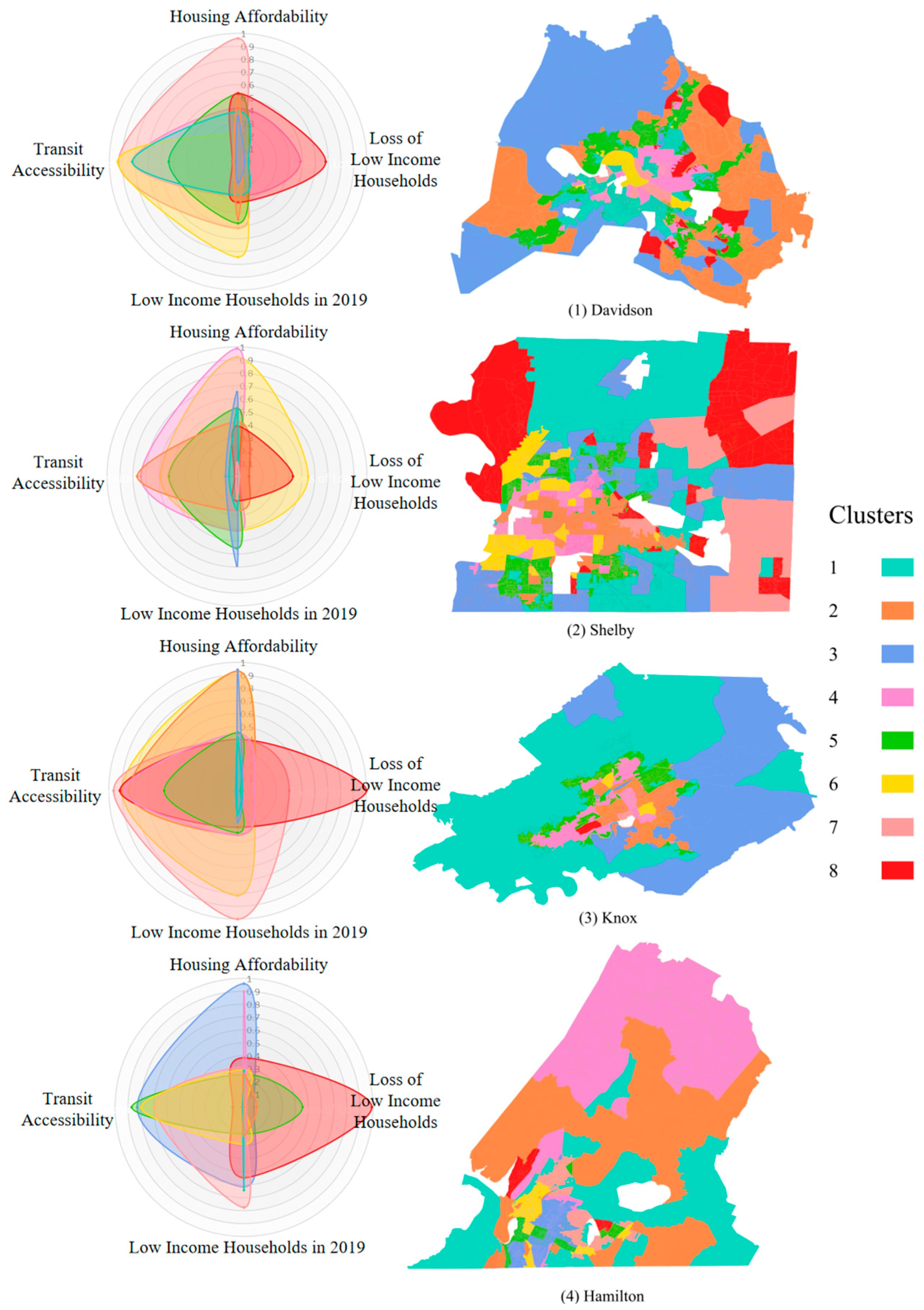
To provide a comprehensive spatial classification, Multivariate Cluster Typology Analysis was conducted using the K-means clustering algorithm. This approach grouped census blocks into eight clusters based on their levels of displacement, transit accessibility, and housing affordability. The optimal number of clusters was determined based on the ratio of between-group to total sum of squares, complemented by considerations of interpretability and meaningfulness of the results. Each cluster was characterized by unique combinations of the three variables, capturing distinct spatial typologies. These typologies were visualized using radar charts and spatial maps, facilitating interpretation and aiding in the identification of priority areas for intervention. Given substantial differences across counties in development context, housing market structure, and transit provision, the cluster analysis was conducted separately for each county to ensure that the resulting typologies reflect locally relevant patterns rather than being constrained by uniform classifications across heterogeneous settings.

5. Results and Discussion

This section presents the results and discussions in four parts. The first part provides the descriptive statistics for the main variables. The second part visualizes the spatial distribution of transit accessibility, housing affordability, and the displacement of low-income households across the four largest counties in Tennessee. The third part focuses on the estimation results from the negative binomial models. The fourth part delves into the spatial results, with a detailed discussion on Bivariate LISA analysis, followed by multivariate cluster typology analysis, highlighting the spatial patterns observed and identifying areas of concern.

5.1. Descriptive Statistics

The distribution of census blocks categorized by income and housing affordability varies significantly across Tennessee’s four largest counties, as shown in

Table 2. Income categories and housing affordability.

Variables		All Counties		Davidson		Shelby		Knox		Hamilton
		(N = 42,858)		(N = 10,222)		(N = 16,179)		(N = 8059)		(N = 8398)
		#	%	#	%	#	%	#	%	#	%
Income category
2010	Low-income	11,628	27.1	2462	24.1	4882	30.2	2054	25.5	2230	26.6
	Mixed low-income	2578	6.0	640	6.3	1188	7.3	454	5.6	296	3.5
	Mixed moderate-income	12,912	30.1	3821	37.4	3281	20.3	3027	37.6	2783	33.1
	Mixed high-income	3110	7.3	1085	10.6	846	5.2	373	4.6	806	9.6
	High-income	12,630	29.5	2214	21.7	5982	37	2151	26.7	2283	27.2
2019	Low-income	10,915	25.5	1370	13.4	5910	36.5	1729	21.5	1906	22.7
	Mixed low-income	3051	7.1	433	4.2	1017	6.3	964	12	637	7.6
	Mixed moderate-income	13,355	31.2	3775	36.9	3658	22.6	2761	34.3	3161	37.6
	Mixed high-income	3021	7.0	891	8.7	740	4.6	575	7.1	815	9.7
	High-income	12,516	29.2	3753	36.7	4854	30	2030	25.2	1879	22.4
Housing affordability in 2019
Housing affordable to:	Low-income	7786	18.2	553	5.4	3610	22.3	1924	23.9	1699	20.2
	Mixed low-income	2178	5.1	98	1.0	541	3.3	901	11.2	638	7.6
	Moderate-income	9633	22.5	2839	27.8	5303	32.8	777	9.6	714	8.5
	Mixed moderate-income	19,568	45.7	4969	48.6	4966	30.7	4380	54.3	5253	62.6
	Housing affordable to mixed moderate-income households	Mixed high-income	5.1	1044	10.2	1039	6.4	0.0	0.0	94	1.1
	High-income	1516	3.5	719	7	720	4.5	77	1	0	0
Displacement (2010–2019)
Blocks without loss of low-income households		27,000	63.0	5068	49.6	11,440	70.7	4475	55.5	6017	71.6
Blocks with loss of low-income households		15,858	37.0	5154	50. 4	4739	29.3	3584	44.5	2381	28.4

#: Frequency; %: Percent.

. Between 2010 and 2019, the proportion of low-income blocks increased in Shelby County (which contains the City of Memphis), whereas Davidson County (which contains the City of Nashville) saw an increase in high-income blocks, reflecting contrasting trends among the counties. Housing affordability also varied notably across counties. Overall, 23.3% of blocks in all four counties had affordable housing for low-income or mixed low-income households. However, Davidson County had the lowest proportion (5.5%), suggesting limited housing affordability, while Knox County was the most affordable, with 35.1% of blocks meeting this criterion. Furthermore, Davidson County had the highest proportion of blocks with housing affordable only for high-income or mixed high-income households, indicating significant affordability challenges. These differences also reflect distinct spatial configurations of affordable housing across counties. In Davidson County, housing affordable to low-income or mixed low-income households is more tightly concentrated in the urban core, whereas in Shelby, Knox, and Hamilton counties, affordable housing is more spatially dispersed across both urban and suburban census blocks. This contrast suggests that affordability in Davidson County is more closely constrained to central locations, while other counties exhibit broader spatial availability of lower-cost housing.

Regarding displacement, 37% of blocks across the four counties experienced a loss of low-income households between 2010 and 2019. Notably, over half of the blocks in Davidson County experienced displacement, the highest among the counties. Knox County, despite its higher affordability, also reported substantial displacement.

A summary of key variables is provided in

Table 3. Summary statistics of key variables.

Variables		Davidson (N = 10,222)			Shelby (N = 16,179)			Knox (N = 8059)			Hamilton (N = 8398)
		Min	Max	Mean	Min	Max	Mean	Min	Max	Mean	Min	Max	Mean
Response variables	Low-income HHs	74	1706	669.65	98	1719	722.48	76	2280	697.53	126	1518	754.88
	Low-income HH loss (2010–2019)	0	517	73.09	0	324	35.40	0	589	48.47	0	261	26.97
Transit accessibility variables	Job Accessibility (90 min)	0	437,771	237,725	0	314,498	117,504	0	140,256	51,818	0	126,886	42,814
Housing variables	Low-cost housing units	69.67	1308.02	517.38	72.49	1338.79	570.55	210.95	1708.36	759.14	138.18	1481.00	832.67
	Legacy housing (40+ years)	0	549	123.22	0	1062	124.67	0	664	111.71	0	375	117.15
	Median gross rent	244.00	3115.00	1165.45	590.00	2012.00	1031.70	374.00	1750.00	899.70	569.00	2118.00	882.13
Socioeconomic variables	Transit commuters	0	696	108.45	0	392	40.06	0	734	35.68	0	568	47.25
	Minority population (%)	1.22	93.11	32.34	1.89	100	60.30	0.00	74.75	14.23	0.00	91.73	25.08
	Bachelor’s degree or higher (%)	1.00	65.00	31.47	1.00	68.00	20.51	3.00	59.00	22.92	1.00	54.00	21.58

. Davidson County experienced the highest average displacement, with 73 households lost per census block, while Hamilton County recorded the lowest displacement rate, averaging 27 households per block. In terms of transit accessibility, Davidson County had the highest levels, both in mean and maximum accessibility, followed by Shelby, Knox, and Hamilton counties. However, Davidson County also had fewer low-cost housing units and higher gross rents compared to the other counties, indicating unique challenges in housing affordability. The table also highlights demographic factors influencing the distribution of low-income households. Davidson County, with the highest transit accessibility, also had the largest average number of transit commuters. Shelby County had the highest proportion of minority residents, while Knox County had the smallest. Additionally, Davidson County reported the highest average proportion of individuals with a bachelor’s degree or higher (31.47%), further distinguishing its socio-economic profile from the other counties.

5.2. Visualizations of Spatial Distribution

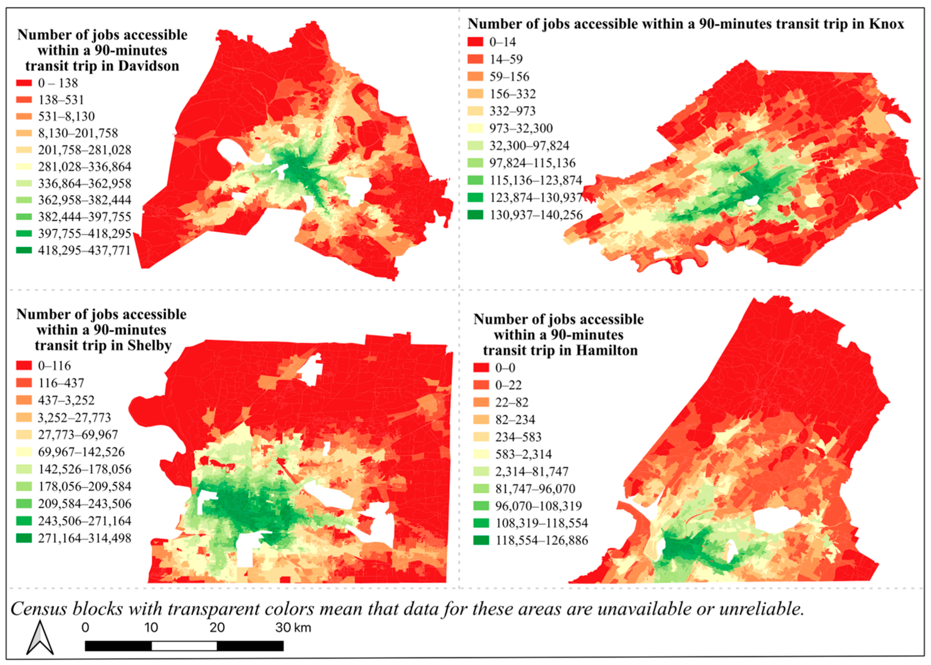
The number of jobs accessible within a 90 min transit trip on a typical weekday is illustrated in Figure 5. The legend for each map uses quantile classification, ensuring equal distribution of values across levels. The maps indicate a general decline in transit accessibility from urban centers to suburban areas. Notably, Hamilton County, which includes the City of Chattanooga, exhibits the highest proportion of blocks with zero transit access, likely due to limited coverage of transit services.

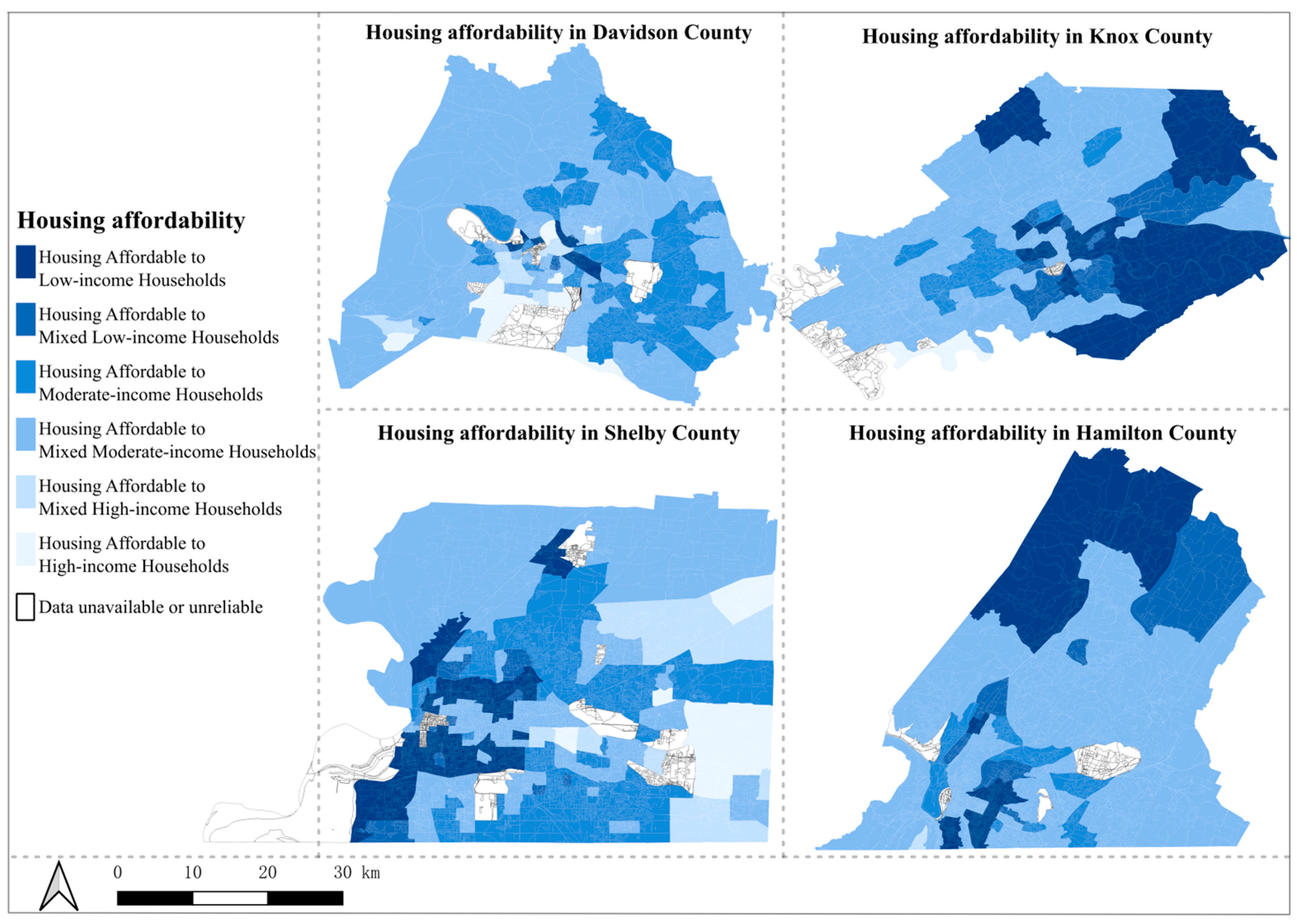
The spatial distribution of affordability levels is presented in Figure 6 using a sequential blue gradient. On this scale, the darkest blue corresponds to level 6, indicating the most affordable housing (affordable to low-income households), while the lightest blue corresponds to level 1, indicating the least affordable housing (affordable to high-income households). The observed spatial patterns reflect the spatial distribution of housing affordability as defined by the relationship between household income and housing costs. The visualization reveals distinct spatial patterns across the study area. In Davidson County, housing affordable to low-income or mixed low-income households is concentrated in fewer census blocks in the urban core, indicating that affordability is achieved in more spatially limited areas. In contrast, Shelby, Knox, and Hamilton counties exhibit a more dispersed pattern, suggesting that a broader range of locations meets the affordability criteria under the same definition. These differences indicate county-level variation in how housing costs and income levels align spatially, resulting in distinct affordability outcomes.

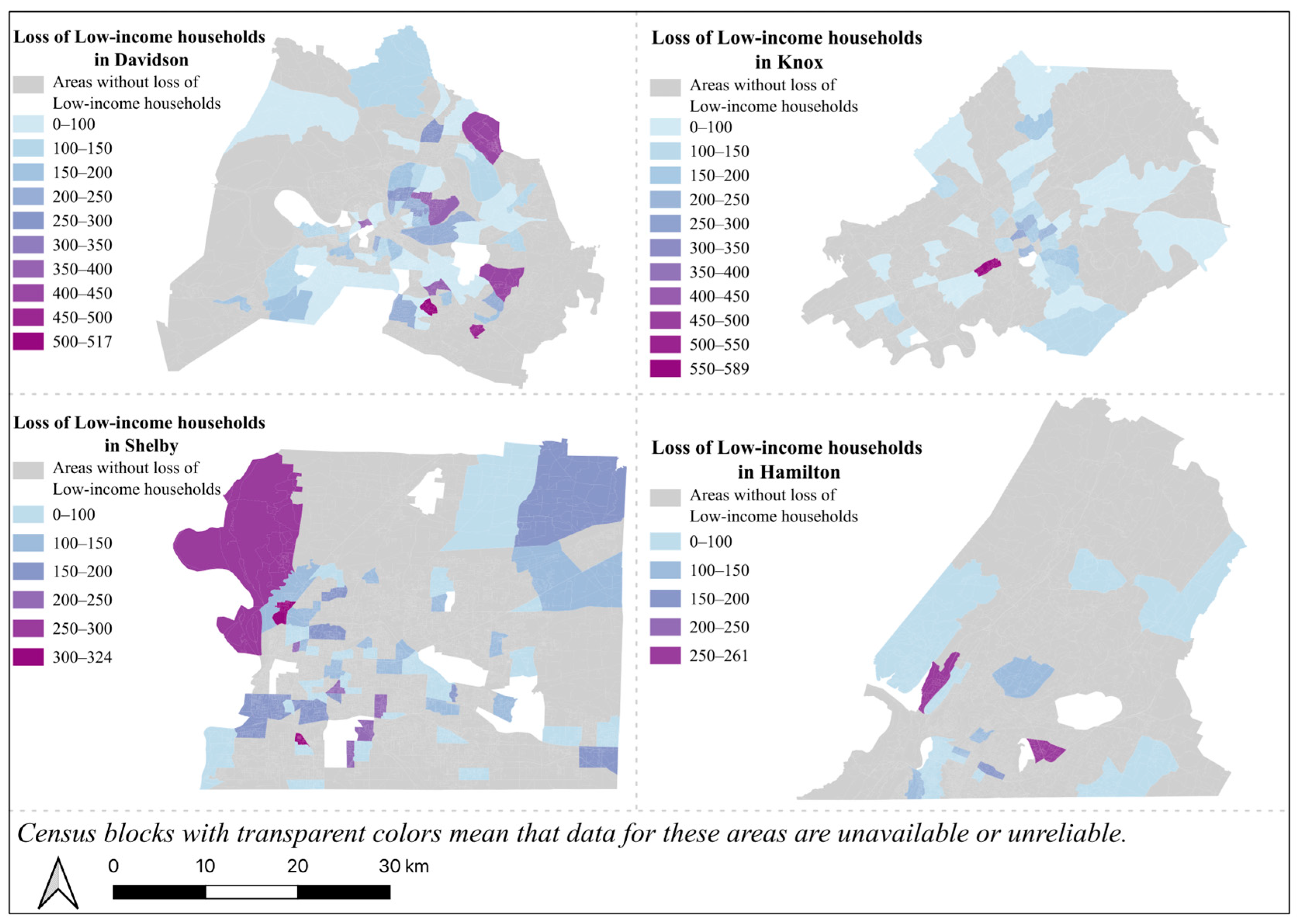
The spatial distribution of low-income household displacement between 2010 and 2019 is depicted in Figure 7. Notably, the displaced households are primarily located in regions with “higher” transit accessibility levels, rather than the absolute “highest” zones. This distinction is critical: the “highest” accessibility areas typically correspond to the commercial Central Business District (CBD), where residential density is lower and market saturation has likely already occurred. Consequently, the wave of displacement is most pronounced in the “higher” accessibility zones—the transit-rich residential neighborhoods immediately adjacent to the core—where gentrification pressures are currently transforming the housing stock. This observation prompts an exploration of the relationship between transit accessibility, housing affordability, and displacement, which is further discussed in the following section.

5.3. Statistical Modeling Results

This section summarizes the results of regression models, examining the association between transit accessibility, housing affordability, and the distribution and displacement of low-income households. The statistical analysis is intended to identify patterns and relationships, without making claims about direct causality.

The estimation results from the negative binomial models are displayed in

Table 4. Negative binomial model for count of low-income households in 2019.

	All Counties (1)		Davidson (2)		Shelby (3)		Knox (4)		Hamilton (5)
	(N = 42,858)		(N = 10,222)		(N = 16,179)		(N = 8059)		(N = 8398)
	$\mathit{\beta }$	SE	$\mathit{\beta }$	SE	$\mathit{\beta }$	SE	$\mathit{\beta }$	SE	$\mathit{\beta }$	SE
Transit accessibility
Jobs accessible within 90 min	0.064 ***	0.0021	0.049 ***	0.0033	−0.076 ***	0.0045	0.538 ***	0.0089	0.234 ***	0.0111
Housing
Low-cost housing units	0.365 ***	0.0021	0.439 ***	0.0052	0.377 ***	0.0037	0.414 ***	0.0046	0.339 ***	0.0032
Housing units 40 years or older	−0.020 ***	0.0019	−0.009 *	0.0038	−0.034 ***	0.0027	−0.072 ***	0.0045	0.105 ***	0.0044
Demographic
Median gross rent	−0.009 ***	0.0025	0.027 ***	0.0053	−0.140 ***	0.0045	−0.076 ***	0.0057	0.144 ***	0.0052
Percent of minority population	0.174 ***	0.0023	0.062 ***	0.0075	0.240 ***	0.0044	0.126 ***	0.0082	0.111 ***	0.0059
Percent of bachelor’s degree or above	0.022 ***	0.0026	−0.040 ***	0.0062	0.151 ***	0.0042	−0.074 ***	0.0042	−0.155 ***	0.0051
Count of workers commuting by transit	0.009 ***	0.0020	0.040 ***	0.0036	−0.049 ***	0.0047	−0.103 ***	0.0048	−0.076 ***	0.0036
Constant	6.491 ***	0.0017	6.554 ***	0.0056	6.458 ***	0.0041	6.610 ***	0.0064	6.541 ***	0.0062
$a$ (Dispersion coefficient)	0.119 ***	0.0008	0.123 ***	0.0017	0.118 ***	0.0013	0.063 ***	0.0010	0.061 ***	0.0010
Log-likelihood with constant only	−309,848.940		−73,569.056		−117,427.028		−57,796.526		−60,855.933
Log-likelihood at convergence	−292,006.244		−69,095.616		−110,305.177		−52,264.365		−54,980.112
p-value for Omnibus Test	0.000		0.000		0.000		0.000		0.000

* p < 0.05; *** p < 0.001. Note: Income and rent were adjusted for inflation.

and

Table 5. Negative binomial model for displacement from 2010 to 2019.

	All Counties (1)		Davidson (2)		Shelby (3)		Knox (4)		Hamilton (5)
	(N = 42,858)		(N = 10,222)		(N = 16,179)		(N = 8059)		(N = 8398)
	$\mathit{\beta }$	SE	$\mathit{\beta }$	SE	$\mathit{\beta }$	SE	$\mathit{\beta }$	SE	$\mathit{\beta }$	SE
Transit accessibility
Jobs accessible within 90 min	0.214 ***	0.0214	0.103 ***	0.0285	0.029	0.0564	1.593 ***	0.1016	−1.718 ***	0.1786
Housing
Low-cost housing units	−0.481 ***	0.0243	−0.580 ***	0.0497	−0.432 ***	0.0490	−0.141 **	0.0541	−1.444 ***	0.0766
Housing units 40 years or older	0.328 ***	0.0209	0.146 ***	0.0334	0.508 ***	0.0431	0.123 *	0.0538	0.806 ***	0.1099
Demographic
Median gross rent	−0.110 ***	0.0213	−0.134 **	0.0433	−0.081	0.0453	−0.836 ***	0.0622	1.003 ***	0.1627
Percent of minority population	−0.380 ***	0.0253	−0.676 ***	0.0703	−0.661 ***	0.0669	−1.190 ***	0.0911	2.526 ***	0.1764
Percent of bachelor’s degree or above	−0.270 ***	0.0286	−0.418 ***	0.0546	−0.805 ***	0.0687	−0.167 ***	0.0467	1.330 ***	0.0760
Count of workers commuting by transit	0.202 ***	0.0202	0.041	0.0305	0.169 ***	0.0487	0.099 *	0.0454	−0.299 *	0.1457
Constant	3.668 ***	0.0165	3.988 ***	0.0431	3.568 ***	0.0496	3.137 ***	0.0767	4.121 ***	0.1352
$a$ (Dispersion coefficient)	11.665 ***	0.1049	7.284 ***	0.1169	15.973 ***	0.2606	7.689 ***	0.1501	13.834 ***	0.3240
Log-likelihood with constant only	−129,635.520		−40,583.507		−40,442.081		−27,638.114		−19,901.939
Log-likelihood at convergence	−129,122.004		−40,440.367		40,241.919		−27,212.382		−19,531.548
p-value for Omnibus Test	0.000		0.000		0.000		0.000		0.000

* p < 0.05; ** p < 0.01; *** p < 0.001. Note: Income and rent were adjusted for inflation.

. Models (1) and (6) include all four counties, while Models (2) to (5) and (7) to (10) analyze each county separately. Prior to model estimation, multicollinearity among explanatory variables was assessed using the Variance Inflation Factor (VIF), and all VIF values were below 5, indicating that multicollinearity was not a concern. The significant dispersion parameters confirm that the negative binomial specification is more appropriate than the Poisson model, given the presence of overdispersion in the data. The log-likelihood values at convergence are considerably higher than those of the constant-only models, indicating that the inclusion of explanatory variables substantially improves model fit. Furthermore, the Omnibus tests are highly significant (p < 0.001), demonstrating that the set of predictors collectively provides strong explanatory power. Besides transit accessibility and housing affordability, the models also consider other factors, such as race and education, that may be associated with the distribution and displacement of low-income households.

5.3.1. Regression Analysis of the Count of Low-Income Households in 2019

The results from five negative binomial models analyzing the distribution of low-income households by census block in 2019 are presented in Table 4. The response variable in these models is the number of low-income households in each block. The coefficient for transit accessibility shows that, except for Shelby County, job access by transit is positively associated with the number of low-income households. This observation is consistent with previous studies indicating that low-income households often reside in areas with better transit access [30,44]. Additionally, the number of low-cost housing units is positively associated with the number of low-income households across all counties. This pattern suggests that low-income households are more prevalent in areas combining relatively higher transit accessibility and more affordable housing options. The results also show that a higher percentage of minority residents corresponds to a greater number of low-income households in all counties. The relationship between education level and the distribution of low-income households varies by county. In Davidson, Knox and Hamilton counties, areas with higher percentages of residents with a bachelor’s degree or higher tend to have fewer low-income households, while the opposite is true for Shelby County. The negative correlation is consistent with traditional patterns of residential segregation. In these regions, educational attainment serves as a strong proxy for higher socioeconomic status, resulting in a spatial structure where highly educated households are concentrated in areas distinct from low-income communities. However, the positive relationship diverges from typical segregation patterns and may reflect the presence of mixed-income dynamics often found in transitional urban neighborhoods. Alternatively, this correlation could be influenced by local institutional factors, such as university districts, where populations in Shelby County with high educational attainment coexist with households reporting lower current incomes. The relationship between the number of transit commuters and the number of low-income households also differs among the counties. In Davidson County, areas with higher numbers of transit commuters tend to have more low-income households, whereas the opposite effect is observed in the other three counties.

5.3.2. Regression Analysis of the Loss of Low-Income Households from 2010 to 2019

The results of five negative binomial models examining the displacement of low-income households from 2010 to 2019 are presented in Table 5. The results reveal distinct regional dynamics regarding the influence of transit accessibility. In Shelby County, transit accessibility is not significantly associated with the loss of low-income households. This lack of significance suggests that in Shelby’s distinct urban context, displacement pressures may be driven more by other factors rather than transit proximity. In contrast, Davidson and Knox counties show a significant positive relationship, where areas with higher transit accessibility experienced greater declines in low-income households. This pattern aligns with “transit-induced gentrification,” common in rapidly growing housing markets. In these counties, high transit accessibility likely acts as a premium amenity, attracting higher-income residents and driving up housing costs, which subsequently displaces lower-income populations who originally relied on the service. Conversely, in Hamilton County, higher job access by transit corresponds to a smaller decline in low-income households. This inverse relationship indicates that in Hamilton, the transit system functions primarily as a stabilizing economic resource. In a potentially less overheated housing market, the cost savings provided by transit access may outweigh rent pressures, allowing low-income households to retain their housing and remain in the neighborhood.

The results also indicate that a greater number of low-cost housing units is associated with less displacement, as indicated by the significant negative coefficients across all counties. This aligns with prior studies linking displacement patterns to rising housing prices driven by transit development [45,46].

Other variables are also associated with displacement patterns. An increase in the number of older housing units corresponds to greater displacement in all counties. Regarding race and education, higher percentages of minority residents or those with bachelor’s degrees (or higher) are linked to greater displacement in Hamilton County, while the opposite pattern is observed in other counties.

While these statistical models identify significant relationships between transit accessibility, housing affordability, and low-income household dynamics, they do not establish causal associations. Many of these associations could be influenced by unobserved factors such as local policies, economic trends, or neighborhood characteristics. Therefore, Section 5.4 complements this analysis by providing qualitative and contextual interpretation of the observed statistical patterns, helping to explore potential mechanisms and contextual factors behind these correlations.

5.4. Spatial Modeling Results

5.4.1. Bivariate LISA

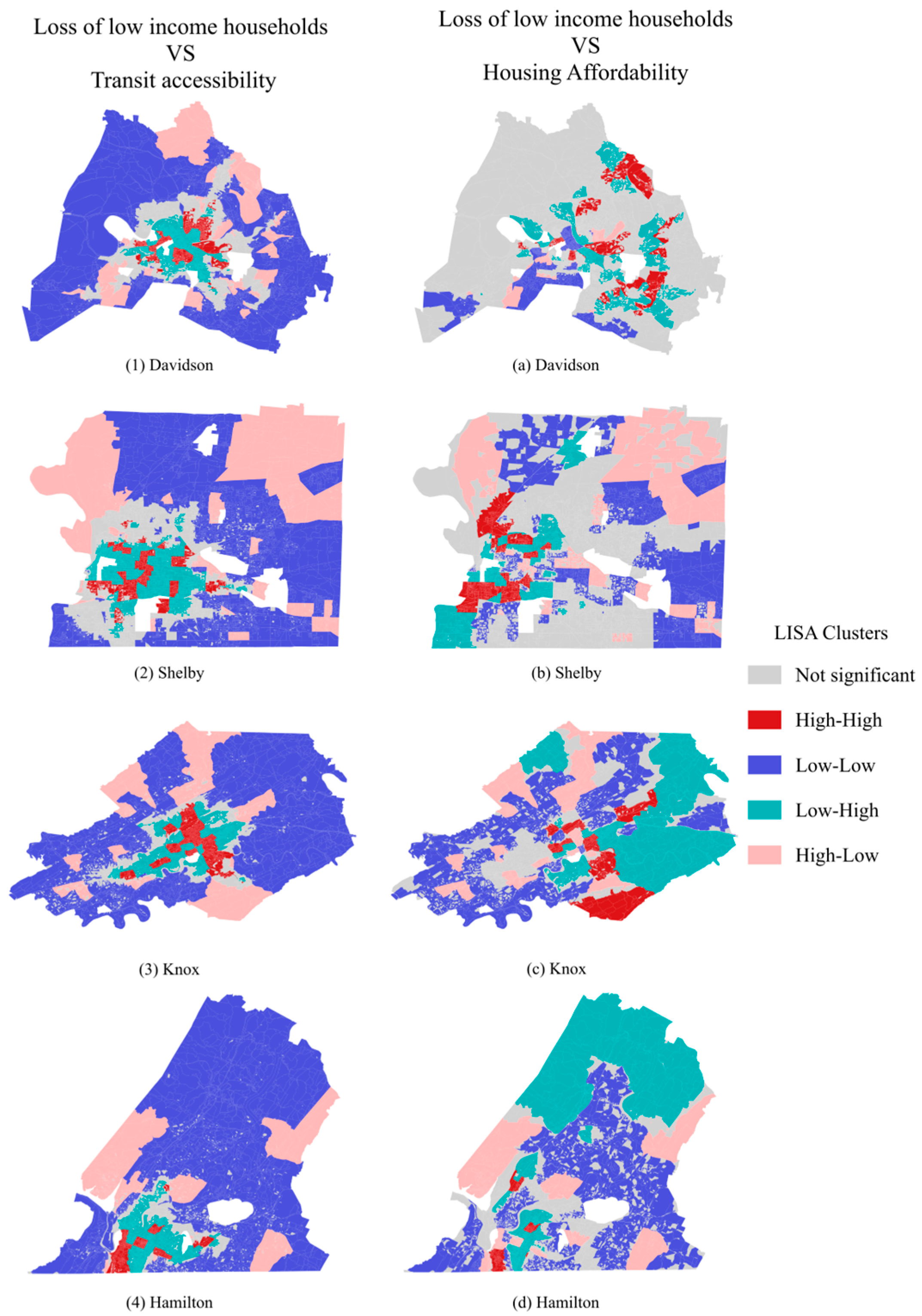
The bivariate LISA maps presented in Figure 8 illustrate the spatial relationships between displacement (measured by the loss of low-income households) and two variables-transit accessibility (left column) and housing affordability (right column) across Davidson, Shelby, Knox, and Hamilton counties. Census blocks are categorized into four significant spatial correlation clusters based on a 5% significance level for local Moran’s I. Blocks with p-values above this threshold are classified as not significant (presented in gray).

The matched correlation clusters include H-H clusters (shown in red), representing areas with both high levels of low-income household loss and high transit accessibility or housing affordability. These regions suggest potential displacement risks in areas where accessibility or affordability conditions are favorable but may still be inaccessible to low-income households due to other socio-economic pressures. Conversely, L-L clusters (indicated in blue) denote blocks with both low levels of low-income household loss and poor transit accessibility or housing affordability, typically stable areas with minimal displacement. The mismatched patterns consist of L-H clusters (indicated in indigo), which highlight regions with low levels of low-income household loss but high transit accessibility or housing affordability. These areas, often considered opportunity areas, suggest that favorable accessibility or affordability conditions may have mitigated displacement. In contrast, H-L clusters (shown in pink) are of particular concern, as they reflect areas where high levels of low-income household loss coincide with either limited transit accessibility or low housing affordability. In these contexts, inadequate accessibility or affordability can act as structural drivers of displacement, identifying priority zones for policy intervention. By contrast, H-H clusters also indicate significant loss, but their favorable accessibility or affordability conditions suggest that displacement there is more strongly linked to broader market dynamics and thus less amenable to direct intervention.

Across all four counties, the spatial patterns of displacement versus transit accessibility display a relatively consistent structure. H-H clusters, representing areas with both high displacement and high transit accessibility, are predominantly distributed in city centers. These areas are characterized by higher transit service density, indicating that low-income households previously residing in certain city center areas with high transit accessibility have experienced significant displacement. While the displacement in these areas is substantial, the presence of already strong transit infrastructure limits the scope for intervention through accessibility improvements.

L-L clusters, reflecting low displacement and low transit accessibility, dominate the outskirts of the cities or suburban peripheries. These areas appear more stable, with fewer signs of population displacement and less-developed transit services. Meanwhile, H-L clusters, indicating areas with high displacement but poor transit accessibility, are also observed in the city outskirts but are less prevalent than L-L clusters. This distribution suggests that regions with low transit accessibility are generally associated with lower levels of displacement, though there are exceptions where underserved areas also experience displacement pressures.

L-H clusters, which reflect low displacement paired with high transit accessibility, are sporadically distributed around the city center or near the boundaries of urban and suburban zones. These areas may represent transitional zones with potential to stabilize low-income populations due to their accessibility advantages.

Unlike displacement versus transit accessibility, the spatial patterns of displacement versus housing affordability exhibit less regularity across the four counties. First, it is evident that the number of insignificant blocks varies among the counties. This variation indicates a weaker spatial correlation between the loss of low-income households and housing affordability in Davidson County, followed by Shelby County, while Knox and Hamilton counties exhibit more blocks with significant spatial correlation between the two variables.

For Davidson County, high-high (H-H) clusters are scattered near the city center, as well as in the northeastern and middle-eastern areas, reflecting irregular patterns of high displacement associated with areas of high housing affordability. However, in Shelby and Hamilton counties, H-H clusters are primarily concentrated near the city center. In Knox County, in addition to being distributed near the city center, H-H clusters are also observed in the southern areas.

Low-high (L-H) clusters in Davidson County exhibit a distribution pattern similar to H-H clusters, indicating that areas with higher housing affordability tend to be clustered together. In Shelby County, most L-H clusters are located near H-H clusters, but a small portion is distributed in the northern part of the county. In Knox and Hamilton counties, L-H clusters extend beyond the city centers and are widely distributed on the outskirts. This suggests that while higher housing affordability might provide some stability for low-income households, it is not uniformly effective across spatial contexts. The peripheral distribution of L-H clusters in Knox and Hamilton counties may reflect a shift in housing affordability dynamics towards suburban areas, potentially driven by urban sprawl or policy interventions.

The clusters with low housing affordability (Low-Low clusters and High-Low clusters shown as blue and pink) highlight areas where unaffordable housing has differing impacts on low-income household displacement. In Davidson County, unaffordable housing in the city center and parts of the middle-southern areas appears to have displaced low-income households significantly. Similarly, in other counties, high displacement is observed in city center areas with low housing affordability. This suggests that in urban cores, low-income households are particularly vulnerable to displacement when housing becomes unaffordable, likely due to competition with higher-income groups and limited access to affordable alternatives.

The differing spatial patterns between displacement and housing affordability, compared to those observed with transit accessibility, highlight the complex interplay of factors influencing the displacement of low-income households. To further explore these dynamics, the next section focuses on a multivariate cluster typology analysis using the K-means clustering method. This analysis aims to integrate multiple variables, including transit accessibility, housing affordability, and displacement patterns, to identify distinct typologies of urban areas. By examining these typologies, we can gain a deeper understanding of the combined effects of these factors on low-income household displacement and uncover potential spatial trends and policy implications.

5.4.2. Multivariate Cluster Typology Analysis

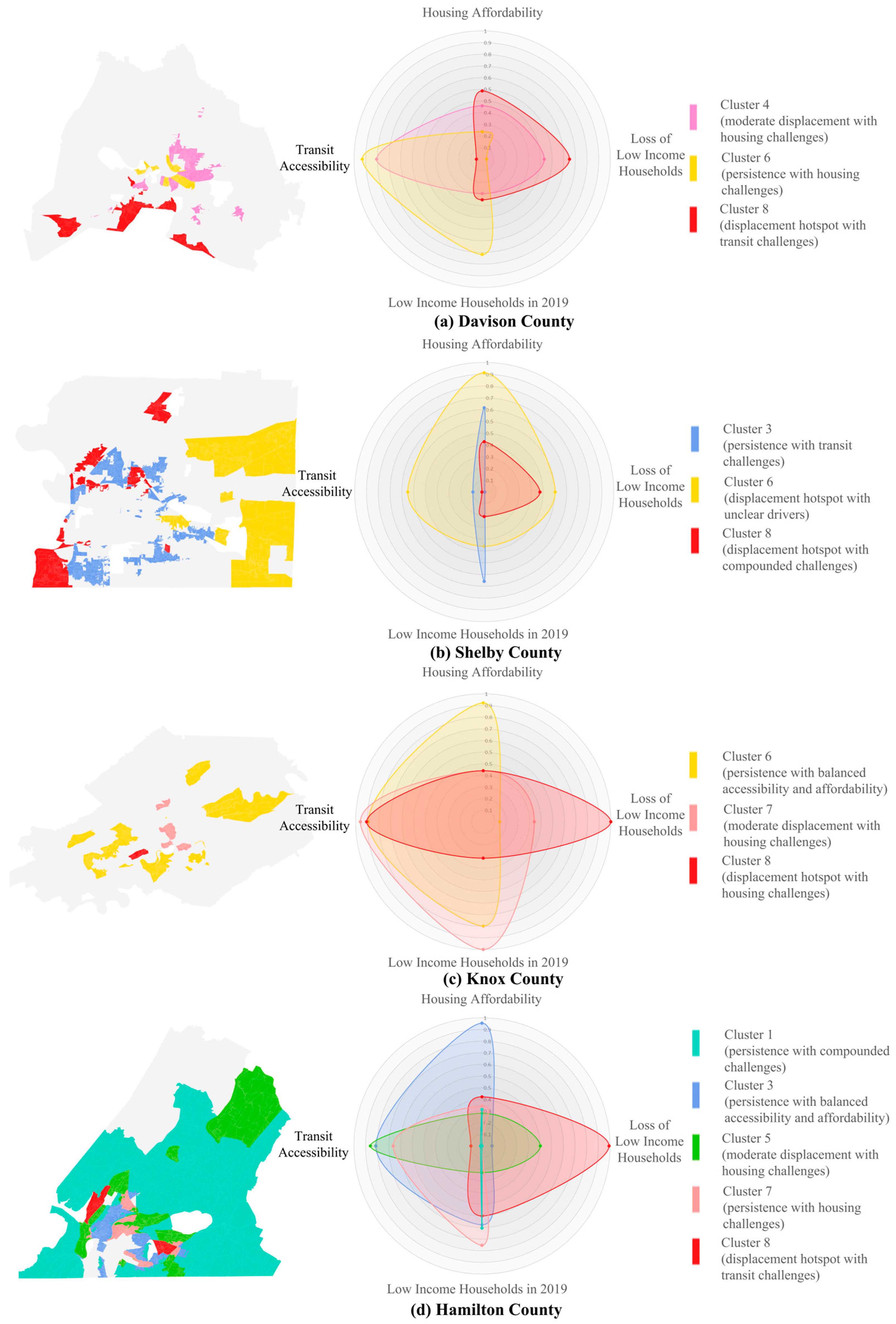
The results of a multivariate cluster typology analysis conducted across four counties using the K-means clustering algorithm are presented in Figure 9. This analysis classifies areas within each county based on four key indicators: transit accessibility, housing affordability, the loss of low-income households from 2010 to 2019, and the concentration of low-income households in 2019. The typology identifies clusters with distinct combinations of these factors, including patterns of significant displacement, persistence in low-income household concentrations, and varying conditions of transit accessibility and housing affordability. Radar charts illustrate the defining characteristics of each cluster, while spatial maps highlight their geographic distributions, offering a detailed understanding of local challenges. To further improve readability, Figure 10 provides a set of radar charts (panels a–d) summarizing only the distinct cluster patterns emphasized in the discussion for each county, together with corresponding county-level maps that display the spatial locations of these clusters. This figure highlights the most relevant typologies and presents them with both cluster numbers and descriptive labels, facilitating clearer cross-county comparisons.

In Davidson County (Figure 10a), two displacement-prone clusters emerge. Cluster 8 (displacement hotspot with transit challenges), highlighted in red, experienced the highest loss of low-income households. Characterized by low transit accessibility, medium housing affordability, and low concentrations of low-income households in 2019, this cluster is located outside the city center, where limited transit services appear to exacerbate displacement. In contrast, Cluster 4 (moderate displacement with housing challenges), marked in light purple, also experienced significant displacement but with medium-to-high transit accessibility. This suggests that housing affordability, rather than transit access, is the key driver of displacement. Geographically, Cluster 4 is concentrated closer to the city center. Meanwhile, Cluster 6 (persistence with housing challenges), shown in yellow, exhibits high concentrations of low-income households in 2019 and near-zero displacement over the past decade. With high transit accessibility but low housing affordability, this cluster indicates that access to transit likely plays a decisive role in retaining low-income populations in the face of affordability challenges.

In Shelby County (Figure 10b), distinct patterns of displacement emerge. Cluster 6 (displacement hotspot with unclear drivers), shown in yellow, experienced the highest loss of low-income households despite very high housing affordability and reasonable transit accessibility, suggesting that other displacement factors require further investigation. This cluster is located to the north and south of the city center. Cluster 8 (displacement hotspot with compounded challenges), shown in red, mirrors Davidson County’s Cluster 8, with very low transit accessibility and medium housing affordability driving displacement. These areas are distributed outside the city center, where insufficient transit and unaffordable housing create significant barriers for low-income households. On the other hand, Cluster 3 (persistence with transit challenges), represented in blue, maintains a high concentration of low-income households in 2019 with low displacement. This cluster demonstrates reasonable housing affordability but very low transit accessibility, suggesting that improving transit access could further stabilize these areas.

In Knox County (Figure 10c), Cluster 8 (displacement hotspot with housing challenges), marked in red, experienced the highest displacement. Located west of the city center, this cluster has high transit accessibility but low housing affordability. Cluster 7 (moderate displacement with housing challenges), highlighted in pink, shows moderate displacement near the city center, with very high transit accessibility, medium housing affordability, and a high concentration of low-income households in 2019. These two clusters indicate that housing costs are likely the main driver of displacement in Knox County. Meanwhile, Cluster 6 (persistence with balanced accessibility and affordability), represented in yellow, exhibits near-zero displacement and high concentrations of low-income households. Benefiting from both high transit accessibility and high housing affordability, this cluster offers a stable environment for low-income populations.

Finally, in Hamilton County (Figure 10d), displacement hotspots and stable areas are evident. Cluster 8 (displacement hotspot with transit challenges), shown in red, experienced the highest displacement, with very low transit accessibility and medium housing affordability. These areas, located to the north and east of the city center, highlight the role of insufficient transit services in displacement. Cluster 5 (moderate displacement with housing challenges), marked in green, shows moderate displacement with low concentrations of low-income households in 2019, despite high transit accessibility. Located in and around the city center, this cluster underscores the impact of housing affordability challenges. In contrast, Cluster 7 (persistence with housing challenges), shown in pink, and Cluster 3 (persistence with balanced accessibility and affordability), shown in blue, exhibit near-zero displacement and high concentrations of low-income households in 2019. Both clusters are located near the city center and benefit from high transit accessibility, though housing affordability is a greater concern in Cluster 7. Lastly, Cluster 1 (persistence with compounded challenges), marked in teal, demonstrates near-zero displacement and high concentrations of low-income households, despite very low transit accessibility and low housing affordability. Located on the county outskirts, this cluster highlights the resilience of low-income populations in peripheral areas, even under compounded challenges.

A comparative analysis of the four counties highlights significant regional variations in the interplay between displacement, transit accessibility, and housing affordability. Davidson and Hamilton Counties exhibit displacement hotspots predominantly driven by either solely transit challenges or solely housing affordability issues. In contrast, displacement hotspots in Knox County, such as Cluster 8, are primarily linked to housing affordability challenges, despite these areas benefiting from relatively high transit accessibility. This suggests that even in transit-accessible areas, rising housing costs can remain a dominant factor driving displacement, underscoring the critical role of affordability in this region. Shelby County, however, presents a more complex scenario, with displacement hotspots such as Cluster 8 reflecting compounded challenges where the drivers of displacement are less clear or involve overlapping factors, including both housing- and transit-related issues.

In summary, while housing affordability remains a crucial factor across all counties, the influence of transit accessibility varies significantly by region. These findings highlight the need for tailored policy interventions that address the unique challenges faced by each county. For displacement hotspots driven solely by transit challenges, such as Cluster 8 in Davidson County and Hamilton County, targeted investments in transit infrastructure are essential, with an emphasis on increasing transit services in areas where affordable housing exists. In areas where displacement is predominantly driven by housing affordability challenges, such as Cluster 4 in Davidson, Cluster 8 in Knox, and Cluster 5 in Hamilton, developing affordable housing programs in transit-robust areas should take precedence. For displacement hotspots with compounded challenges, such as Shelby County’s Cluster 8, further investigation is required to evaluate the trade-offs and design multi-dimensional strategies that address both housing affordability and transit accessibility barriers comprehensively.

For persistent areas not experiencing significant displacement despite transit or housing challenges, such as Shelby’s Cluster 3, enhancing transit services or improving housing conditions could strengthen their stability. By addressing these varying dynamics with tailored strategies, policymakers can more effectively mitigate displacement and support equitable and sustainable urban development.

6. Conclusions

This study examined how transit accessibility and housing affordability are related to the distribution and displacement of low-income households across the four largest counties in Tennessee. By integrating negative binomial regression with spatial analyses, including Bivariate LISA and multivariate cluster typology analysis, the study links county-wide statistical relationships with localized spatial patterns of displacement.

The regression results indicate substantial regional variation in displacement dynamics. In Davidson and Knox Counties, higher transit accessibility is associated with greater losses of low-income households between 2010 and 2019, whereas in Hamilton County, higher job access by transit corresponds to lower displacement. Across all counties, a higher number of low-cost housing units is consistently associated with greater retention and higher concentrations of low-income households. These findings underscore that transit accessibility does not exert a uniform influence on displacement and that housing supply plays a critical stabilizing role. Differences in the effects of demographic variables, such as education and minority composition, further highlight the importance of county-specific contexts.

Spatial analyses deepen these insights by identifying localized patterns that are not evident from regression results alone. Bivariate LISA reveals clusters where high displacement coincides with either limited transit accessibility or housing affordability constraints. Multivariate cluster typology analysis further classifies census blocks into distinct displacement-related typologies, capturing complex combinations of transit conditions, housing affordability, and low-income household presence. Together, these spatial findings demonstrate that displacement pressures are highly uneven within counties and arise through different mechanisms depending on local conditions.

From a sustainability perspective, these results emphasize that equitable and sustainable urban development requires coordinated consideration of both transportation and housing systems. Transit investments that are not accompanied by adequate housing affordability protections may unintentionally intensify displacement, undermining social sustainability and long-term community stability. Conversely, areas where affordable housing and transit access coexist show greater capacity to retain low-income households, supporting inclusive and resilient urban systems. The findings therefore highlight the need for place-sensitive strategies that align transit planning with housing affordability goals to promote sustainable urban development.

7. Limitations and Future Work

This study has several limitations that point to directions for future research. First, displacement was measured using aggregate changes in the number of low-income households, which does not capture individual relocation trajectories or motivations. Future studies could incorporate household-level or longitudinal data to better distinguish displacement from other forms of residential mobility. Second, while spatial clustering was explicitly analyzed, the regression models did not account for spatial dependence. Applying spatial regression techniques could further clarify the interaction between neighboring areas. Third, this analysis focused on four counties in Tennessee, and the findings may not be directly transferable to regions with different transit systems or housing markets. Expanding this framework to additional metropolitan areas would help assess its broader applicability. Finally, the study period predates the COVID-19 pandemic, and future research should examine whether post-pandemic shifts in transit use and housing markets have altered displacement dynamics.

References

1. Freeman, L. Displacement or succession? Residential mobility in gentrifying neighborhoods. Urban Aff. Rev. 2005, 40, 463–491. [Google Scholar] [CrossRef]
2. Pasha, O.; Wyczalkowski, C.; Sohrabian, D.; Lendel, I. Transit effects on poverty, employment, and rent in Cuyahoga County, Ohio. Transp. Policy 2020, 88, 33–41. [Google Scholar] [CrossRef]
3. Zahertar, A.; Lavrenz, S. Transit and Bikeshare Connectivity in Detroit: New Insights on Socioeconomic and Infrastructure Factors Impacting Perceived Quality of Service. J. Urban Mobil. 2025, 7, 100120. [Google Scholar] [CrossRef]
4. Cong, W.; Zhou, J.; Lai, Y. The coordination between citywide rail transit accessibility and land-use characteristics in Shenzhen, China: An explorative analysis based on multidimensional spatial data. Sustain. Cities Soc. 2024, 113, 105691. [Google Scholar] [CrossRef]
5. Shakespeare, R.M. Mapping the desirable and affordable city: Middle-income renter perceptions of housing opportunity. Urban Geogr. 2025, 46, 1408–1431. [Google Scholar] [CrossRef]
6. Anselin, L. Local indicators of spatial association—LISA. Geogr. Anal. 1995, 27, 93–115. [Google Scholar] [CrossRef]
7. Macioszek, E.; Świerk, P.; Grana, A.; Sobota, A. Application of a Logit Model to Identify Socio-Demographic Factors Influencing the Choice of Public Transport for Daily Trips—A Case Study Based on the Example of the Górnośląska-Zagłębiowska Metropolis (Poland). Transp. Probl. Int. Sci. J. 2024, 19, 183. [Google Scholar]
8. Zuk, M.; Bierbaum, A.H.; Chapple, K.; Gorska, K.; Loukaitou-Sideris, A. Gentrification, displacement, and the role of public investment. J. Plan. Lit. 2018, 33, 31–44. [Google Scholar] [CrossRef]
9. Easton, S.; Lees, L.; Hubbard, P.; Tate, N. Measuring and mapping displacement: The problem of quantification in the battle against gentrification. Urban Stud. 2020, 57, 286–306. [Google Scholar]
10. Carlson, H.J. Measuring displacement: Assessing proxies for involuntary residential mobility. City Community 2020, 19, 573–592. [Google Scholar] [CrossRef]
11. Desmond, M.; Shollenberger, T. Forced displacement from rental housing: Prevalence and neighborhood consequences. Demography 2015, 52, 1751–1772. [Google Scholar] [CrossRef] [PubMed]
12. Martin, I.W.; Beck, K. Gentrification, property tax limitation, and displacement. Urban Aff. Rev. 2018, 54, 33–73. [Google Scholar] [CrossRef]
13. Wyly, E.; Newman, K.; Schafran, A.; Lee, E. Displacing new york. Environ. Plan. A Econ. Space 2010, 42, 2602–2623. [Google Scholar] [CrossRef]
14. Ellen, I.G.; O’Regan, K.M. How low income neighborhoods change: Entry, exit, and enhancement. Reg. Sci. Urban Econ. 2011, 41, 89–97. [Google Scholar] [CrossRef]
15. McKinnish, T.; Walsh, R.; White, T.K. Who gentrifies low-income neighborhoods? J. Urban Econ. 2010, 67, 180–193. [Google Scholar] [CrossRef]
16. Chapple, K.; Thomas, T.; Zuk, M. Urban Displacement Project. Available online: https://www.urbandisplacement.org/ (accessed on 20 June 2024).
17. Chapple, K.; Zuk, M. Forewarned: The use of neighborhood early warning systems for gentrification and displacement. Cityscape 2016, 18, 109–130. [Google Scholar]
18. El-Geneidy, A.; Levinson, D.; Diab, E.; Boisjoly, G.; Verbich, D.; Loong, C. The cost of equity: Assessing transit accessibility and social disparity using total travel cost. Transp. Res. Part A Policy Pract. 2016, 91, 302–316. [Google Scholar] [CrossRef]
19. Ermagun, A.; Tilahun, N. Equity of transit accessibility across Chicago. Transp. Res. Part D Transp. Environ. 2020, 86, 102461. [Google Scholar] [CrossRef]
20. Stewart, A.F. Mapping transit accessibility: Possibilities for public participation. Transp. Res. Part A Policy Pract. 2017, 104, 150–166. [Google Scholar] [CrossRef]
21. Zhou, T.; Liu, D.; Liu, W.; Li, Y.; Zhu, S.; Wang, J.; Shi, L. Hierarchical dynamic estimation of fire service accessibility based on POI big data. Case Stud. Therm. Eng. 2024, 59, 104503. [Google Scholar] [CrossRef]
22. Wessel, N.; Farber, S. On the accuracy of schedule-based GTFS for measuring accessibility. J. Transp. Land Use 2019, 12, 475–500. [Google Scholar] [CrossRef]
23. Hu, L.; Liao, Y.; Gao, K.; Jin, S.; Precup, R.-E. Integration of e-scooter sharing with public transit on employment accessibility and equity. Transp. Res. Part D Transp. Environ. 2025, 140, 104604. [Google Scholar] [CrossRef]
24. Conway, M.W.; Stewart, A.F. Getting Charlie off the MTA: A multiobjective optimization method to account for cost constraints in public transit accessibility metrics. Int. J. Geogr. Inf. Sci. 2019, 33, 1759–1787. [Google Scholar] [CrossRef]
25. Stone, M.E. What is housing affordability? The case for the residual income approach. Hous. Policy Debate 2006, 17, 151–184. [Google Scholar] [CrossRef]
26. Galster, G.; Lee, K.O. Housing affordability: A framing, synthesis of research and policy, and future directions. Int. J. Urban Sci. 2021, 25, 7–58. [Google Scholar] [CrossRef]
27. Robinson, M.; Scobie, G.M.; Hallinan, B. Affordability of Housing: Concepts, Measurement and Evidence; New Zealand Treasury Working Paper; New Zealand Government, The Treasury: Wellington, New Zealand, 2006.
28. Meen, G. How should housing affordability be measured. UK Collab. Cent. Hous. Evid. 2018, 3, 3–29. [Google Scholar]
29. Guo, J.; Brakewood, C.; Hightower, A.; Cherry, C. Evaluating equity: A method for analyzing the transit accessibility of affordable housing units. Transp. Res. Rec. 2024, 2678, 668–686. [Google Scholar] [CrossRef]
30. Pathak, R.; Wyczalkowski, C.K.; Huang, X. Public transit access and the changing spatial distribution of poverty. Reg. Sci. Urban Econ. 2017, 66, 198–212. [Google Scholar] [CrossRef]
31. Tao, S.; Cheng, L.; He, S.; Witlox, F. Examining the non-linear effects of transit accessibility on daily trip duration: A focus on the low-income population. J. Transp. Geogr. 2023, 109, 103600. [Google Scholar] [CrossRef]
32. Barton, M.S.; Gibbons, J. A stop too far: How does public transportation concentration influence neighbourhood median household income? Urban Stud. 2017, 54, 538–554. [Google Scholar] [CrossRef]
33. Higgins, C.D.; Arku, R.N.; Farber, S.; Miller, E.J. Modelling changes in accessibility and property values associated with the King Street Transit Priority Corridor project in Toronto. Transp. Res. Part A Policy Pract. 2024, 190, 104256. [Google Scholar]
34. Debrezion, G.; Pels, E.; Rietveld, P. The impact of railway stations on residential and commercial property value: A meta-analysis. J. Real Estate Financ. Econ. 2007, 35, 161–180. [Google Scholar]
35. Jin, T.; Cheng, L.; Liu, Z.; Cao, J.; Huang, H.; Witlox, F. Nonlinear public transit accessibility effects on housing prices: Heterogeneity across price segments. Transp. Policy 2022, 117, 48–59. [Google Scholar] [CrossRef]
36. Hensley, V. “State of Emergency”: Edgehill, Nashville, Tennessee and the Fight Against Displacement from Urban Renewal to Gentrification. Doctoral Dissertation, Middle Tennessee State University, Murfreesboro, TN, USA, 2022. [Google Scholar]
37. Welch, J.G.; Sims, C.B.; McKinney, M.L. Does an urban wilderness promote gentrification? A case study from Knoxville, Tennessee, USA. Sustainability 2022, 14, 973. [Google Scholar] [CrossRef]
38. Chen, Y.; Jia, S.; Xu, Q. Evaluating the accessibility and equity of key amenities in the X-minute and Y-monetary-cost city: A double-threshold cumulative opportunity measure. J. Public Transp. 2025, 27, 100128. [Google Scholar] [CrossRef]
39. Kim, J.; Lee, B. More than travel time: New accessibility index capturing the connectivity of transit services. J. Transp. Geogr. 2019, 78, 8–18. [Google Scholar] [CrossRef]
40. Boisjoly, G.; Moreno-Monroy, A.I.; El-Geneidy, A. Informality and accessibility to jobs by public transit: Evidence from the São Paulo Metropolitan Region. J. Transp. Geogr. 2017, 64, 89–96. [Google Scholar] [CrossRef]
41. Fransen, K.; Neutens, T.; Farber, S.; De Maeyer, P.; Deruyter, G.; Witlox, F. Identifying public transport gaps using time-dependent accessibility levels. J. Transp. Geogr. 2015, 48, 176–187. [Google Scholar] [CrossRef]
42. Chang, L.Y. Analysis of freeway accident frequencies: Negative binomial regression versus artificial neural network. Saf. Sci. 2005, 43, 541–557. [Google Scholar] [CrossRef]
43. Wallace, B.; Mannering, F.; Rutherford, G.S. Evaluating effects of transportation demand management strategies on trip generation by using Poisson and negative binomial regression. Transp. Res. Rec. 1999, 1682, 70–77. [Google Scholar] [CrossRef]
44. Glaeser, E.L.; Kahn, M.E.; Rappaport, J. Why do the poor live in cities? The role of public transportation. J. Urban Econ. 2008, 63, 1–24. [Google Scholar] [CrossRef]
45. Cappellano, F.; Spisto, A. Transit oriented development & social equity: From mixed use to mixed framework. Adv. Eng. Forum 2014, 11, 314–322. [Google Scholar] [CrossRef]
46. Rayle, L. Investigating the connection between transit-oriented development and displacement: Four hypotheses. Hous. Policy Debate 2015, 25, 531–548. [Google Scholar] [CrossRef]
Figure 1. Location of the study area.
Sustainability 18 00859 g001
Figure 2. Chart of income category classification.
Sustainability 18 00859 g002
Figure 3. Chart of housing affordability classification. *** Housing Affordable to.
Sustainability 18 00859 g003
Figure 4. Workflow chart.
Sustainability 18 00859 g004
Figure 5. Spatial distribution of transit accessibility in the four counties.
Sustainability 18 00859 g005
Figure 6. Spatial distribution of housing affordability in the four counties.
Sustainability 18 00859 g006
Figure 7. Spatial distribution of the displacement of low-income households in the four counties.
Sustainability 18 00859 g007
Figure 8. Bi-LISA cluster maps for loss of low-income households and transit accessibility or housing affordability.
Sustainability 18 00859 g008
Figure 9. Radar charts and maps of multivariate K-means clustering results.
Sustainability 18 00859 g009
Figure 10. Radar charts and maps of distinct cluster typologies.
Sustainability 18 00859 g010