Field-Scale Techno-Economic Assessment and Real Options Valuation of Carbon Capture Utilization and Storage—Enhanced Oil Recovery Project Under Market Uncertainty

Abstract

This study develops a field-based techno-economic model and decision framework for a CO₂-enhanced oil recovery and storage project under joint market uncertainty. Historical drilling and completion expenditures calibrate investment cost functions, and three years of production data are fitted with segmented hyperbolic Arps curves to forecast 20-year oil output. Markov-chain models jointly generate internally consistent pathways for crude oil, ETA, and purchased CO₂ prices, which are embedded in a Monte Carlo valuation. The framework outputs probability distributions of NPV and deferral option value; under the mid scenario, their mean values are USD 18.1M and USD 2.0M, respectively. PRCC-based global sensitivity analysis identifies the dominant value drivers as oil price, CO₂ price, utilization factor, oil density, pipeline length, and injection volume. Techno-economic boundary maps in the joint oil and CO₂ price space then delineate feasible regions and break-even thresholds for key design parameters. Results indicate that CCUS-EOR viability cannot be inferred from oil price or any single cost factor alone, but requires coordinated consideration of subsurface constraints, engineering configuration, and multi-market dynamics, including the value of waiting in unfavorable regimes, contributing to low-carbon development and sustainable energy transition objectives.

1. Introduction

Carbon Capture, Utilization and Storage (CCUS) is the predominant technique to reduce CO₂ emissions, recognized as a crucial technology that may promote the attainment of a low-emission, secure, and economical energy system [1]. Within the technical framework of CCUS, Enhanced Oil Recovery (EOR) is a technique that fulfils the dual objectives of augmenting crude oil output and sequestering CO₂, thereby establishing itself as the most technologically advanced and extensively advocated CO₂ storage method [2].

The present research concentrates on examining the gas injection mechanism in the CO₂ flooding process from an engineering standpoint [3], alongside the microscopic principles driving CO₂ displacement [4]. Additionally, refs. [5,6] have assessed the process safety of CO₂-EOR concerning wellbore integrity and pipeline corrosion. Conversely, regarding the economic assessment of this project, several studies have analyzed its economic performance using traditional essential indicators such as net present value (NPV), internal rate of return (IRR), and payback period [7]. Others have conducted more comprehensive analyses of the evaluation system for CCUS-EOR [8] and project full life cycle costs and cash flows [9]. However, the existing research has led to a division in geology, engineering, and economics. Most studies in the technical field end with the optimal injection–production plan, and a simple economic evaluation is conducted to prove the economic feasibility, while the studies in the management field have failed to connect the geological and engineering part with the subsequent evaluation, missing analysis of the critical, geological, or engineering parameters influencing the economic performance. Hence, this study addresses the following research question: In what manner do joint market uncertainties, namely oil prices, emission trading allowance prices, and CO₂ purchase prices, alongside engineering design and subsurface limitations, influence the economic feasibility, risk assessment, and optimal deferral decision for a field-scale CO₂-EOR and storage initiative in China?

Therefore, to address the identified gap between subsurface-engineering analysis and decision-oriented economic evaluation amid market uncertainty, this study develops a comprehensive techno-economic assessment and decision-making framework for CCUS-EOR projects. The innovation of this study is not in the Monte Carlo simulation itself, but in the field-scale integration and the decision-oriented results facilitated by a cohesive workflow. Well investment costs and a 20-year oil production profile are calibrated using historical cost and production datasets. Three interrelated market time series—oil prices, emission trading allowance (ETA) prices, and CO₂ prices—are jointly generated via a Markov-based market model and integrated into the economic evaluation framework. Monte Carlo simulation is then employed to quantify the probability distributions of net present value (NPV) and deferral option value. Building on these results, a global sensitivity analysis identifies and ranks the key geological, engineering, and economic drivers, which are further translated into techno-economic feasibility envelopes. These envelopes provide decision-relevant boundary conditions across diverse oil and CO₂ pricing scenarios, offering actionable insights for project stakeholders.

2. Materials and Methods

This study complies the market data and integrates comprehensive life cycle project costs with actual production revenues to construct an economic evaluation model, subsequently employed to simulate and assess the 20-year economics of the supercritical CO₂ recovery project in a low-permeability conglomerate oil reservoir.

2.1. Research System

The research system comprises three phases: capture, transport, and utilization and storage commenced with the CO₂ seller and concluded at the buried reservoir. The costs and profits associated with each phase of the carbon sequestration system constitute the economic framework, where the project’s overall income is quantified by crude oil revenue, and ETA. Simultaneously, the acquisition of CO₂ has served as the exclusive carbon source, without evaluation of expenses linked to capture devices.

2.2. Data Collection

2.2.1. Reservoir Data

To maintain confidentiality, the study location is designated as “Province A”. This study exemplifies a conventional onshore low-permeability conglomerate reservoir in China, with baseline technical and financial assumptions aligned with publicly accessible regional data and the literature. Since the project is a pilot initiative, the CO₂ injection rate is far from reaching the maximum capacity of the injection well, and the injection is inconsistent, resulting in unpredictable and intermittent oil production volume. Consequently, this study has implemented the methodologies from the existing literature to construct the injection and production model.

Given that the reservoir consists of three primary oil horizons with analogous geological features but different depths, this study utilizes the average value shown in Table 1 to integrate them and streamline the model. The project’s well pattern is a five-spot arrangement resulting in an approximate injection–production well ratio of 2.4, based on actual well site data and the findings of [10].

Table 1. Reservoir data. The table shows the crucial parameters of reservoir, along with their symbols and values.

Parameters	Symbol	Value
Permeability	kh	5 md
Thickness	h	20 m
Depth	d	1725 m
Reservoir pressure	Pres	16.3 MPa
Oil density	ρ	0.83 kg/m3

2.2.2. Market Data

Three market data series, namely crude oil price, ETA, and CO₂ price, which serve as the principal indicators of market-side volatility affecting project revenues and partial costs, are introduced.

Revenue Side

The primary revenue of this project derives from the crude oil generated during CO₂ flooding and the earnings from carbon trading associated with carbon storage.

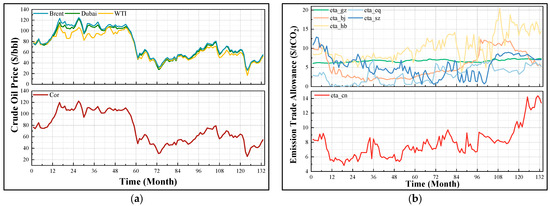
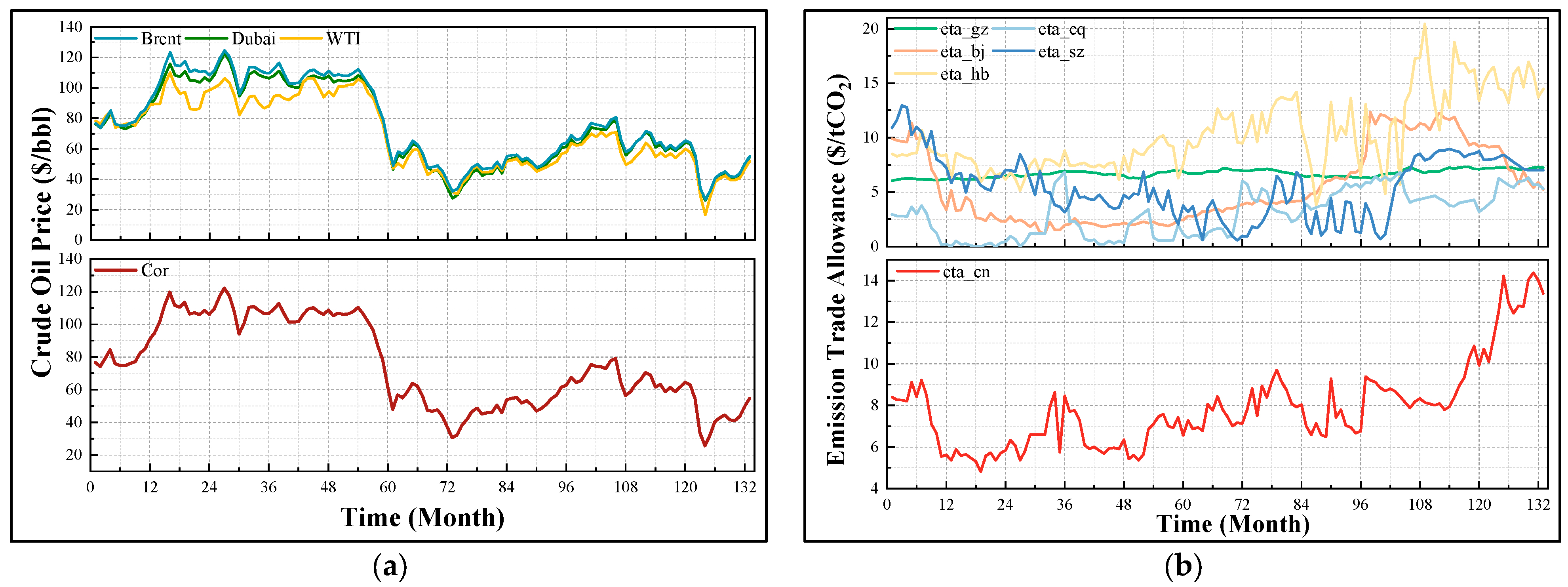
The historical monthly data of crude oil prices from Brent, Dubai, and West Texas Intermediate (WTI), which are three major benchmark crude oil series widely used to represent international oil market conditions, spanning from 2014 to 2025 [11,12,13], about 133 months, are used to comprehensively depict the crude oil price in China. The correlated crude oil price is derived using a 6:3:1 ratio, highlighting the predominant influence of the marine benchmarks of Brent and Dubai, while retaining the marginal insights provided by WTI regarding global supply and demand fluctuations. The data series are shown in Figure 1a, containing the monthly crude oil prices for Brent, Dubai, and WTI, along with their respective correlations as the crude oil price for subsequent work.

Figure 1. Market data related to revenue. (a) Historical monthly data of crude oil prices from Brent, Dubai, WTI, and Cor (Correlated price). (b) Historical monthly data of ETA of each pilot region, and estimated China national ETA.

This work synthesizes the regional pilot ETS data from 2014 to 2015, specifically from Guangzhou, Chongqing, Beijing, Shenzhen, and Hubei [14,15,16,17,18], to represent the nationwide ETS data launched in China in 2021 [19]. In addition, this study has standardized scale and timing across areas to reduce level and volatility variation, subsequently aggregating them into a unified national framework. Figure 1b represents the monthly ETA of each pilot region, and the calculated eta_cn series encapsulates the prevailing market signal while accommodating institutional changes over time.

Hence, the entire revenue could be calculated through the aggregation of two components, illustrated in the equation below.

$$R_i^{tot}=S_i^{oil}{Q}_i^{oil}{\displaystyle \frac{6.29}{\rho }}+S_i^{ETA}{Q}_i^{car}$$

(1)

where $R_i^{tot}$ represents the total revenue in the year i; $S_i^{oil}$ and $S_i^{ETA}$ are the crude oil price and ETA in year i; $Q_i^{oil}$ and $Q_i^{car}$ represent the production of oil and injection of CO₂ in year i; ρ represents the oil density; and 6.29/ρ denotes the ton barrel ratio.

Cost Side

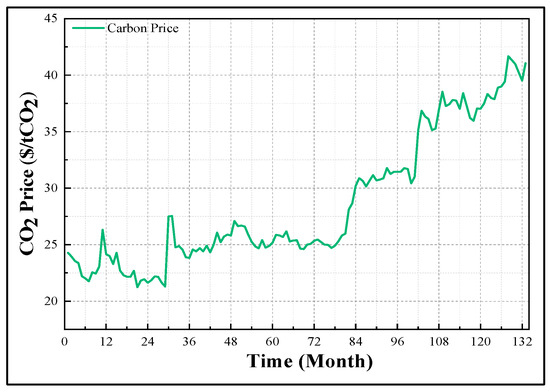
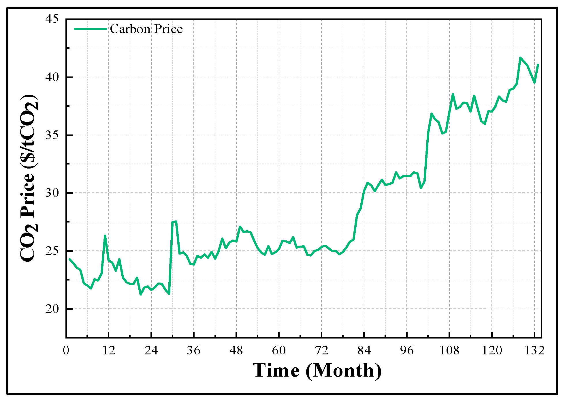
Due to sparse long-run domestic quotations for industrial CO₂, this study has derived a CO₂ price series by integrating the industrial CO₂ price index [20] as the inter-temporal trend proxy and a set of recent domestic monthly quotations [21]. The resulting series reflecting ex-factory pricing is presented in Figure 2.

Figure 2. Historical monthly data of calculated industrial CO₂ price.

Since this study has considered purchasing CO₂ as the sole source, the capital expenditure during the capture phase can be evaluated using the following equation:

$$CAPE{X}_i^{cap}=S_i^{C{O}_2}{Q}_i^{car}$$

(2)

where $S_i^{C{O}_2}$ represents the CO₂ price.

2.2.3. Costs

Costs Within Transport Stage

The costs associated with the transportation phase covers the costs of the pipeline, compressor, and pump. The investment costs of pipelines presume that the economies of scale for an extensive pipeline project, comprising numerous sections with varying diameters, are either equivalent to or just marginally different from those of identical length but with a singular diameter [22]. Consequently, length is the sole parameter considered in this work to derive the capital expenditure (CAPEX) and operation and maintenance (O&M) costs of the pipeline, which can be estimated using the equation proposed by ref. [23].

This work utilizes the simulation of supercritical CO₂ injection, in which CO₂ is compressed from the beginning pressure to the cut-off pressure by compressors. The segmented compression calculation methods are employed to simulate the actual conditions of CO₂ and the required compressors and pumps. Appendix A.1 shows the full calculations for the power requirements of the compressors and pumps, as well as the quantity of compressors needed. Hence, the expenses of compressors and pumps are subsequently concluded based on the injection amount via the following equations [24], and Appendix B.1 shows the full calculations for CAPEX and O&M.

$$CAPE{X}_i^{tran}=CAPE{X}_i^{pipeline}+CAPE{X}_i^{com+pump}$$

(3)

$$O\&M_i^{tran}=O\&M_i^{pipeline}+O\&M_i^{com+pump}+O\&M_i^{elec}$$

(4)

Costs Within Utilization and Storage Stage

The CAPEX throughout the utilization and storage phase may be characterized by the expenses associated with drilling of injection and production wells, fracturing, and ground engineering. Due to the inability to determine a specific ground engineering CAPEX figure per well, the capital could only be evaluated by dividing the total expenditures of the entire sites by the number of wells, resulting in an average of around USD 26.1 per well. Aside from ground engineering CAPEX, the remaining capitals are fit in the next chapter. Appendix A.2 has demonstrate the calculation process for number of injection wells, whereas the number of production well is determined by multiplying the number of injection wells by the injection–production ratio. For the O&M costs, this study has integrated the empirical formulas used in the daily operation of the oilfield with the calculation processes stated by ref. [25]. Appendix B.2 shows the full calculations for CAPEX and O&M.

$$CAPE{X}_i^{stor}=CAPE{X}_i^{id}+CAPE{X}_i^{pd}+CAPE{X}_i^f+CAPE{X}_i^{ge}$$

(5)

$$O\&M_i^{storage}=O\&M_i^{surface}+O\&M_i^{subsurface}+O\&M_i^{others}+O\&M_i^{monitor}$$

(6)

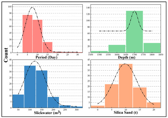
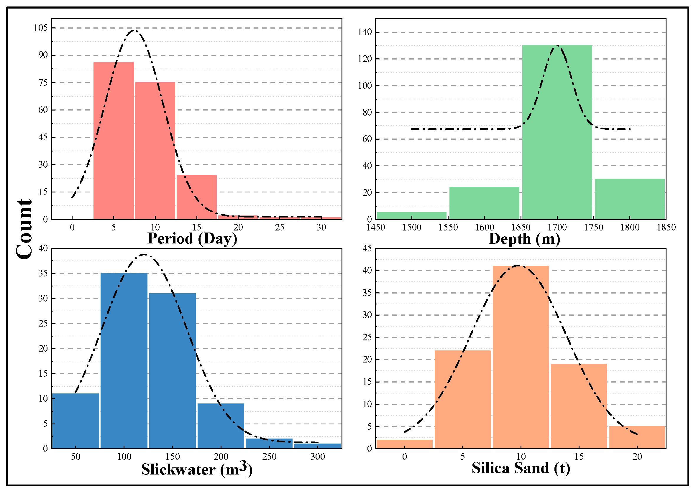
This study simulates the drilling and fracturing costs under different well parameters by fitting the investment data of well engineering. After data collection and cleaning, the drilling CAPEX is fitted for a total of 88 production wells and 101 injection wells. In the injection wells, 89 wells underwent small-scale fracturing, and the data from these wells are used for fracturing CAPEX fitting. The sample range of well engineering parameters related to drilling and fracturing are presented in Figure 3 and Table 2.

Figure 3. Well engineering parameters. The figure demonstrates the distribution of historical data for the four engineering parameters during well completion.

Table 2. Well engineering parameters. This table delineates the principal parameters influencing drilling and fracturing investments, while also indicating the sample size of historical data, the spectrum of parameter values, and the range of concentrations.

Parameter	Symbol	Sample Size	Range	Concentration
Period (Day)	D	189	6–30	5–10
Depth (m)	d	189	1519–1839	1650–1800
Slick water (m3)	SW	89	58–303	100–200
Silica sand (t)	SS	89	2–24	5–15

2.2.4. Tax

The projects are primarily led by oilfield firms, with the discussion on taxes predominantly centered on oilfield taxes during utilization and storage. The CO₂-EOR project tax typically encompasses resource tax, special oil gains, and income tax, as shown in the equation below. The special oil gains are calculated by the crude oil revenue multiplying the results of the subtraction by different levy and deduction groups in different crude oil markets as shown in Table 3.

$${Tax}_{\mathrm{i}}={\tau }^{resource}{S}_i^{oil}{Q}_i^{oil}+{\tau }^{income}EBI{T}_i+(5\cdot {\alpha }_i-{\beta }_i)S_i^{oil}{Q}_i^{oil}$$

(7)

where EBIT_i is the earnings before interests and taxes; τ^resource and τ^income denote resource tax and income tax, valuing at 0.0487 and 0.25, respectively.

Table 3. Levy and deduction rates in the special oil gains. α_i and β_i represent the levy rates and deduction rates in different intervals of crude oil price.

Crude Oil Price (USD/bbl)	Levy Rates (αi)	Deduction Rates (βi)
65	0.2	0
70	0.25	0.25
75	0.3	0.75
80	0.35	1.5
85	0.4	2.5

2.3. Methodology

2.3.1. Production Curve

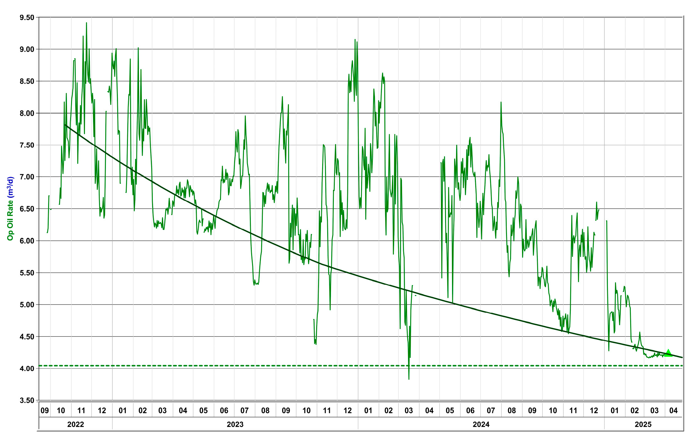
This study has used the Arps decline model to depict the evolution of oil production over time following the implementation of EOR. Specifically, the historical samples consist of daily oil production data from well A, spanning from October 2022 to April 2025, during which EOR was implemented in November 2023, covering a period of about three years. Although the continuous production data are currently inadequate to develop a highly trustworthy numerical reservoir model at the full field scale, this study employs IHS Harmony 2014 v2 to align with the baseline production curve that illustrates the long-term incremental oil production patterns under existing engineering operations, expanding the current model to encompass a 20-year project duration. The fitting results provide a baseline decline model calibrated using field data, rather than an accurate physical prediction of each individual well’s production, as this study primarily emphasizes the subsequent economic analysis of the project.

Considering that the incremental production capacity in the development process of CCUS-EOR may exhibit different diminishing characteristics at different stages, the study has applied segmented hyperbolic decline model instead of single hyperbolic model. The production in a certain stage could be described by the following equation:

$$q_k(t)={\displaystyle \frac{q_k(t_{k-1})}{{(1+b_k{D}_k(t-t_{k-1}))}^{1/b_k}}, }\begin{array}{l}t\in [t_{, k-1},t_k)\\ k=1,2,3\end{array}$$

(8)

where q_k(t_k−1) represents the initial production in the stage k price, with unit t/y; D_k and b_k denote the decline rate and hyperbolic decline exponent; k is the number of stages.

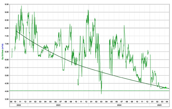
Figure 4 illustrating the two segmented fitting results and Table 4 presenting the decline rate and hyperbolic decline exponent are displayed below. The initial segment pertains to the early reaction phase immediately following the commencement of injection, characterized by a relatively high drop rate (27.04%/y) and a moderate hyperbolic exponent (0.78). The second segment denotes the primary production phase, wherein incremental oil output is maintained over an extended duration, characterized by modest decrease rates (18.83%/y) and a hyperbolic exponent (0.60).

Figure 4. Fitting result according to the historical data. The green solid line represents the historical daily oil production data from late 2022 to early 2025, while the dark green curve signifies the fitted line of the decline model; the green triangle symbol represents the end of history data, and the green dashed line represents the final production rate.

Table 4. Fitting results. The table displays the decline coefficients for each segment of the hyperbolic decline model fitting results, alongside the actual and fitted cumulative production and their respective errors.

Stage	Decline Rate (%/y)	Hyperbolic Exponent	Duration (Month)	Actual Np (103 m3)	Fit Np (km3)	Error (%)
1	27.04	0.78	12.54	2.52	2.52	~1
2	18.83	0.60	17.67	2.25	2.49	~10

The analysis illustrates the project’s oil production volume over 20 years by simulating the oil production curve, using a three-stage decline that features a reduced decline rate and hyperbolic exponent. In the decline model, the decline rates and hyperbolic exponents for the first and second stages are determined based on the aforementioned fitting results, whereas the decline rate and hyperbolic exponent for the third stage are established at values lower than those of the second stage as indicated in [26]. During this experimental operation, approximately 5300 tons of CO₂ were injected in the first year, achieving a utilization factor of nearly 2.64 tCO₂/tOil, slightly above the figure published by refs. [27,28], which employed the same gas injection scheme of alternating water and gas injection, but with a lower permeability. Consequently, this study employed this value as the baseline case to compute the oil yield in the initial year based on the injection volume.

$$Q_0^{oil}={\displaystyle \frac{Q_0^{car}}{\xi }}$$

(9)

where ξ denotes the utilization factor; $Q_0^{oil}$ is the 1st year oil capacity, in the unit of tons.

2.3.2. Economic Evaluation Framework

Scenario Based on Stochastic Market

This study has established scenarios derived from market series, wherein crude oil prices, ETA, and CO₂ pricing are integrated into capital budgeting metrics using quarterly time intervals throughout a project period of 20 years. To illustrate scenario dependence evident in historical data, each series is divided into terciles based on three scenarios: low, mid, and high. The tercile divisions for the market series are determined by the observed values and their sample sizes, yielding the market scenarios presented in Table 5.

Table 5. Market scenarios. The table presents the initial values of the three market series associated with the low, mid, and high scenarios.

Scenario	Oil Price (USD/bbl)	q1/q2	ETA (USD/tCO2)	q1/q2	CO2 Price (USD/tCO2)	q1/q2
Low	47.11	58.80	5.87	6.86	23.55	24.89
Mid	69.65	94.11	7.65	8.27	25.81	30.69
High	107.15		9.15		37.02

This study employed two simulation methodologies, namely static and dynamic models, based on log-return moments and the contemporaneous return correlation matrix for each market interval scenario, thereby situating the project within both static scenario-based and real market contexts. The static method perceives the market as immutable, with the initial market scenario matrix G₀ = {g_oil, g_ETA, g_CO2} maintaining throughout the project’s duration. However, in the dynamic method, the joint scenario matrix is defined as a 1st order and timely homogeneous Markov chain [29], with the transition matrix computed via the same tercile division with Laplace smoothing to suppress the numerical instability caused by zero counting and state sparsity. The dynamic simulation relies on the initial scenario matrix. At each step Δt, the log returns from the preceding state i are extracted from matrix N(μ_i, σ_i), multiplied to update the subsequent state, and then the next state is derived from transition matrix P_i. This method is continuously reiterated to derive a unified trajectory based on the three market series.

$$P_{ij}={\displaystyle \frac{N_{ij}+\alpha }{{\displaystyle {\sum }_{j’}(N_{ij’}+\alpha )}}}$$

(10)

$$r_t^{(x)}=\ln (S_t^x/S_{t+1}^x)$$

(11)

$${\mu }_i^{(x)}={\rm E}[r_t^x\left|G_{t-1}=i\right.] {\sigma }_i^{(x)}=std[r_t^x\left|G_{t-1}=i\right.]$$

(12)

$$S_t^x=S_{t-1}\exp (r_t)$$

(13)

where N_ij and α denote the number of state transitions and a smooth coefficient valuing at 0.5; $r_t^{(x)}$ represents the log return matrix; $S_t^x$, $g_i^x$, ${\mu }_i^{(x)}$, and ${\sigma }_i^{(x)}$ denote prices of market series, scenario, mean, and standard deviation, respectively.

NPV and Option Value

In both static and dynamic approaches, the net present value (NPV) is regarded as the essential criterion for evaluating the project’s economics, determined based on cash flow.

$$C{F}_i=R_i^{tot}-CAPE{X}_i^{cap}-O\&M_i^{tran}-O\&M_i^{stor}-{Tax}_i$$

(14)

$$NPV=-(CAPE{X}_i^{tran}+CAPE{X}_i^{stor})+{\displaystyle \sum _t^{T}C{F}_i{e}^{-rt}}$$

(15)

where CF_i denotes the cash flow in the year i; r represents the discount rate.

As demonstrated by ref. [30], the decision to initiate the project immediately is defined as a discrete-time optimization problem. The approach involves enumerating the permissible investment time points across the three interconnected market scenarios and calculating the option value (OV) by comparing the NPV of immediate investing with the expected value of deferring the decision. The maximum deferral period is five years, and the prime value (PV) is the highest NPV in the deferred choice.

$$NPV(\tau )=-(CAPE{X}_0^{tran}+CAPE{X}_0^{stor})e^{-r\tau \Lambda t}+{\displaystyle \sum _{t=\tau +1}^{T}C{F}_{\tau }{e}^{-rt\Delta t}}$$

(16)

$$PV=\max NPV(\tau )$$

(17)

$$OV=PV-NPV(0)$$

(18)

where τ represents the deferral time; NPV(0) is the NPV investing immediately; Δt represents the step size, valuing at 3 months.

Table 6 delineates the parameters employed in each segment of this model.

Table 6. Parameters in the baseline case involved in the model. The table demonstrates the parameters with their symbols and values in the baseline case.

Parameters	Symbol	Value
1st Decline Rate/Period/ Hyperbolic Factor	D1	27.04%/y
	t1	1 y
	b1	0.78
2nd Decline Rate/Period/Hyperbolic Factor	D2	18.83%/y
	t2	17 y
	b2	0.60
3rd Decline Rate/Period/ Hyperbolic Factor	D3	14%/y
	t3	2 y
	b3	0.55
Utilization factor	ξ	2.64 tCO2/tOil
Duration	D	8 d
Slick water	SW	150 m3
Silica sand	SS	15 t
Out pressure	Pout	13 MPa
Injection amount	$Q_i^{car}$	200,000 t
Pipeline length	L	200 km
Power price	$S_i^p$	0.042 USD/kwh
Discount rate	r	0.12
Project life time	T	20 y
Step time	Δt	0.25 y

3. Results and Discussion

3.1. CAPEX Fitting Results

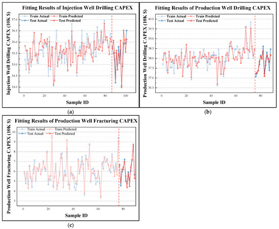
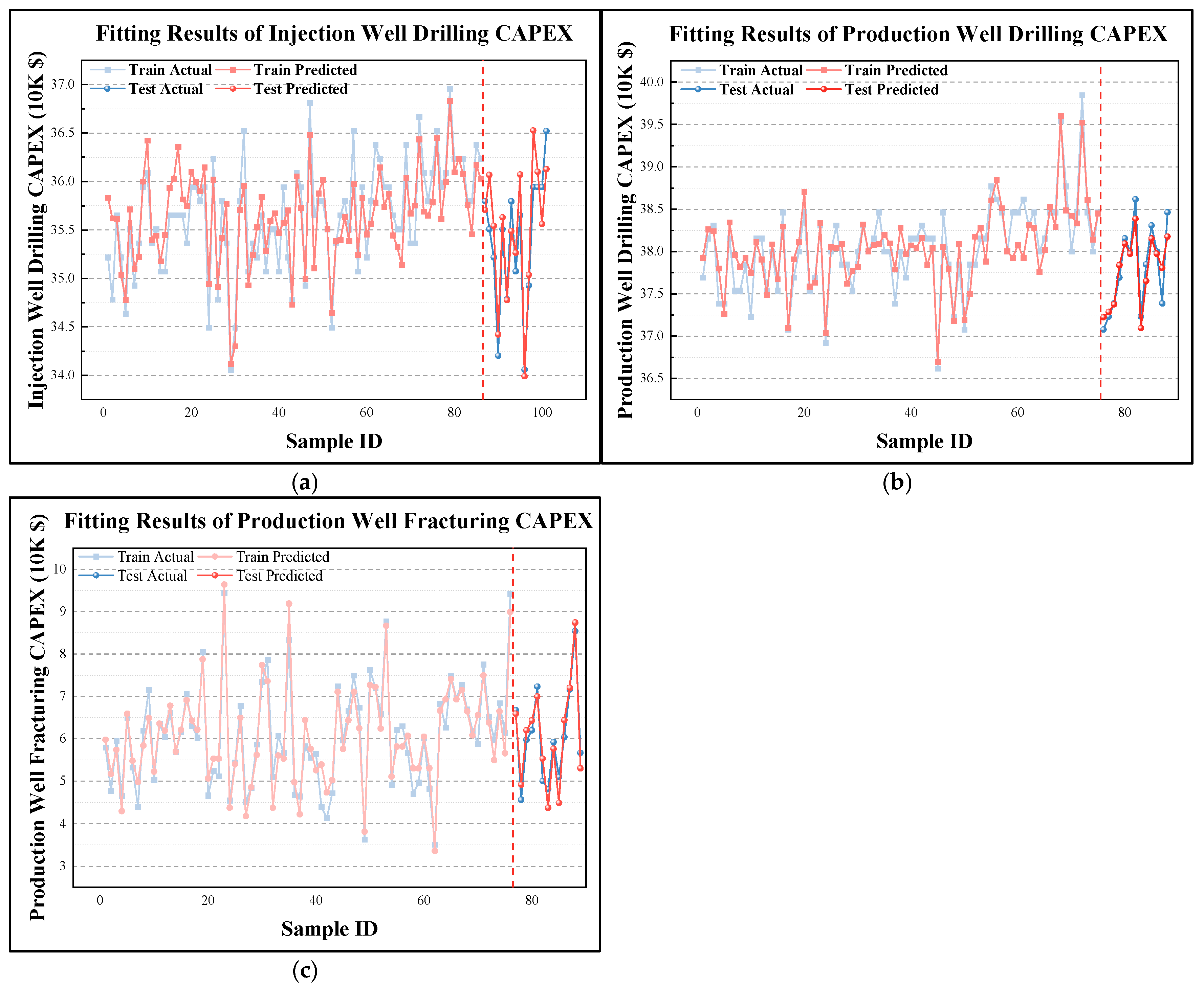
The non-linear and linear models are employed to fit the drilling and fracturing CAPEX, respectively, as all parameters, except for depth, have been linearly influenced by the construction duration, while the fracturing CAPEX is primarily influenced by the quantities of slick water and silica sand utilized. In addition, the models which partition the data into an 85% and a 15% set for training and test to fit, while utilizing K-fold cross-validation (K = 5) on the training set, have been applied to improve robustness. The fitting plots of the drilling CAPEX for injection and production wells and fracturing CAPEX are presented in Figure 5.

Figure 5. (a) Fitting results of injection well drilling CAPEX. (b) Fitting results of production well drilling CAPEX. (c) Fitting results of production well fracturing CAPEX. The light blue line with square markers and the light red line with circular markers represent the training set for actual data and fitting data, while the blue line and the red line with spherical markers denote the test set for actual data and fitting data.

As stated in Table 7, the R²s for the non-linear drilling models for both the training and test sets are higher than 0.7, showing a good fit result, and K’s error is acceptable, and the R²s for test sets of injection and production well drilling CAPEX are in the range of K’s. In addition, the R²s for the linear drilling models for both the training and test sets show fair enough results with 0.911 and 0.902 values, and the K’s error displays a low value, 0.035, which shows a high degree of model explanation. The table below indicates that the R² values for the non-linear drilling models for both the training and testing sets exceed 0.7, demonstrating a satisfactory fit. Additionally, K’s error is deemed acceptable, and the R² levels for the test sets of injection and production well drilling CAPEX align with K’s range. Further, the R² scores for the linear drilling models for both the training and testing sets are adequate at 0.911 and 0.902, whilst the K’s error exhibits an insignificant value of 0.035, signifying a high level of predictive accuracy.

Table 7. Fitting results. The table shows the R², RMSE, and MAE of the training and test sets, and the R² of the K-fold cross-validation of the CAPEX of well construction.

CAPEX	Train/Test/K	R2	RMSE	MAE
Injection Well Drilling	Train	0.738	1.967	1.588
	Test	0.773	2.170	1.812
	K	0.709 ± 0.108
Production Well Drilling	Train	0.794	1.529	1.221
	Test	0.856	1.204	0.850
	K	0.758 ± 0.120
Production Well Fracturing	Train	0.911	2.385	1.958
	Test	0.902	2.196	1.932
	K	0.890 ± 0.035

Hence, the fitting equations of drilling CAPEX for both injection and production wells and fracturing CAPEX are listed below.

$$CAPE{X}_i^{id}=N_i^{inj}(0.47D+200.00e^{0.00018d}-34.19)$$

(19)

$$CAPE{X}_i^{pd}=N_i^{pro}(0.36D+200.00e^{0.00017d}-30.36)$$

(20)

$$CAPE{X}_i^f=N_i^{inj}(0.04SW+1.43SS+15.35)$$

(21)

3.2. Economic Results

3.2.1. Static Result

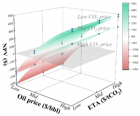
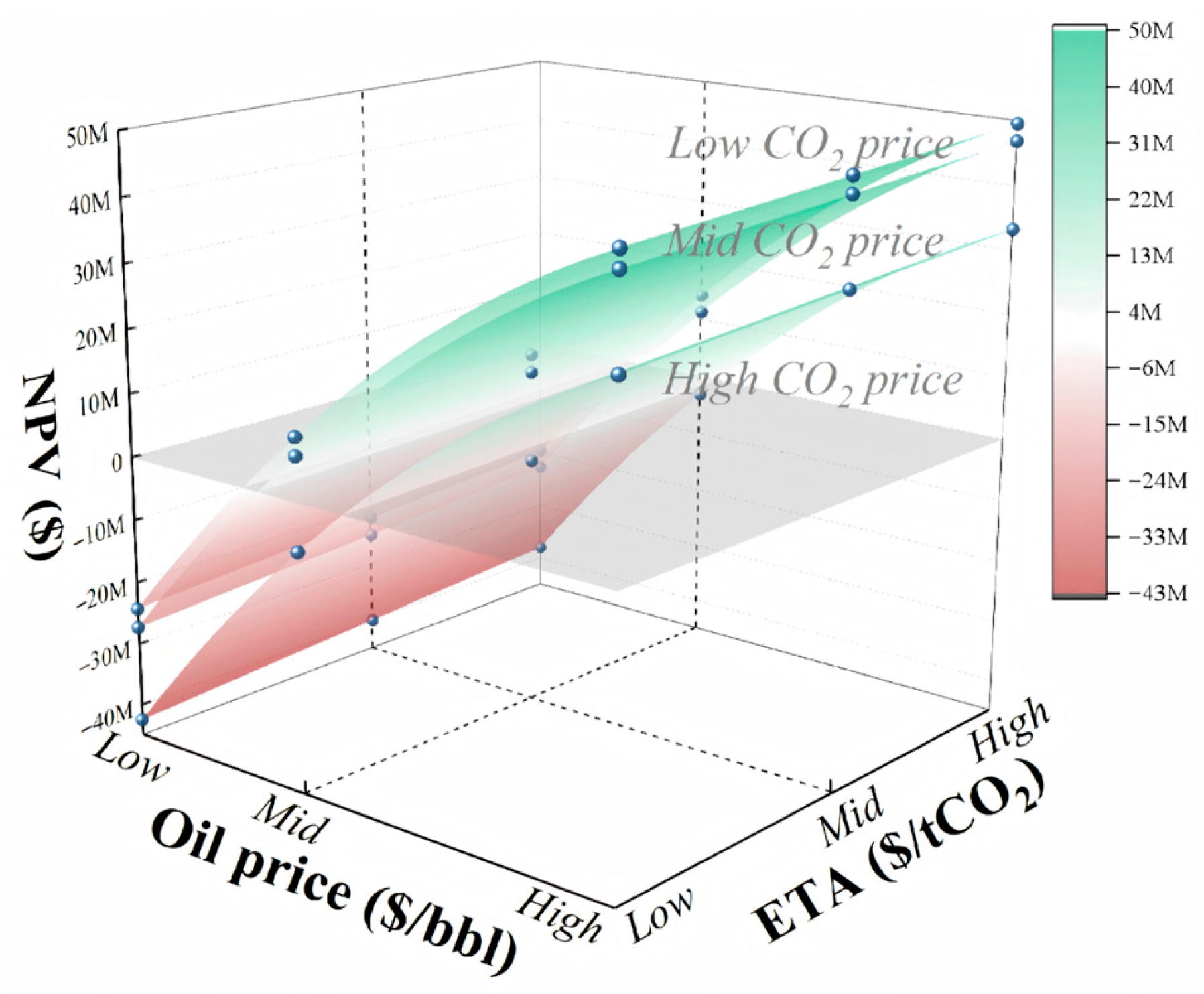
In the static scenario, the market is perceived as stable, with all market variables maintaining their initial values. Figure 6 indicates that the NPV is consistently negative under conditions of low oil prices; there are also situations of high CO₂ prices with mid oil prices. In addition, the impact of rising oil prices on the NPV exhibits a tendency of diminishing returns rather than a straightforward linear relationship, and the NPV increases by around USD 30 million when the oil price attains the next level. The influence of ETA and CO₂ prices on the NPV is linear, with a one-ton variation in the price of ETA and CO₂ leading to an almost USD 1.2 million difference in NPV. Nonetheless, the market fluctuations of ETA and CO₂ prices differ significantly in magnitude as the installation of ETA in China occurred relatively late and the pricing remains lower. Consequently, oil prices and CO₂ purchase prices are the primary factors affecting the NPV, whilst the ETA serves as a supplementary factor that mitigates adverse scenarios.

Figure 6. The NPV of 27 scenarios. The plot depicts the variation in the NPV throughout three market series, with the blue spheres representing 27 scenarios, and the grey plane which denotes the break-even (NPV = 0) threshold.

In conclusion, the findings indicate a highly stable double monotonic structure, wherein the NPV rises with increasing oil prices and decreasing CO₂ purchase prices, while the ETA supplies the secondary buffer. This suggests that given the context of external oil prices, prioritizing low-cost carbon sources and moderately enhancing ETA are two viable methods to maintain the project’s economic performance within a favorable range.

3.2.2. Dynamic Result

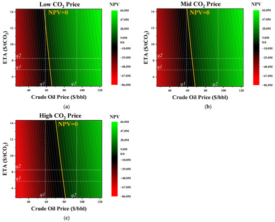
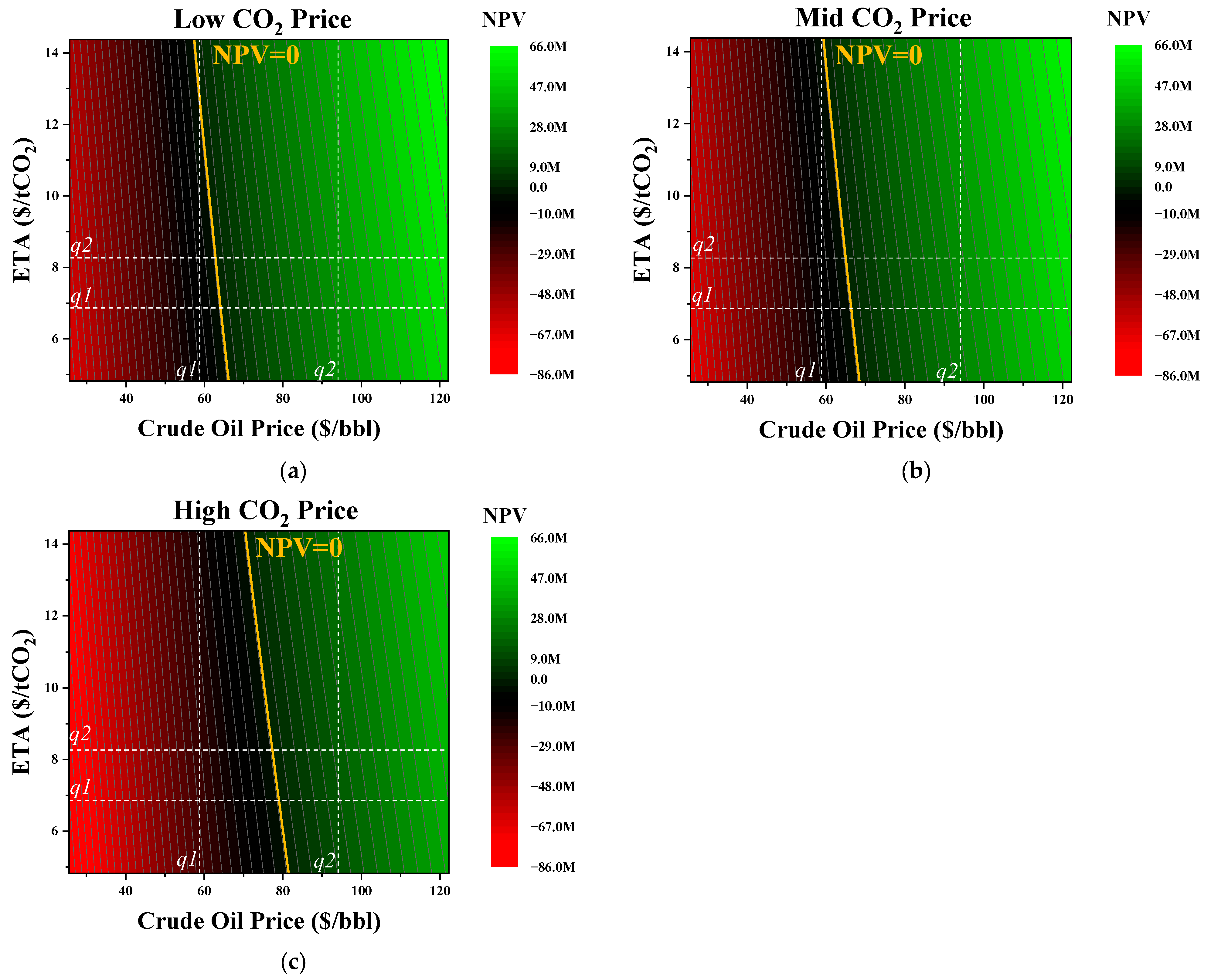
The Monte Carlo simulation utilizing random seed 26 and 10,000 pathways is employed to iteratively generate clusters of market trajectories, which are subsequently utilized for NPV/Option and other statistical evaluations. The study has plotted NPV heat maps for ETA and crude oil price across three CO₂ purchase price, as depicted in Figure 7.

Figure 7. Heat map of the NPV according to crude oil price and ETA in the scenario. (a) Low CO₂ price; (b) mid CO₂ price; and (c) high CO₂ price. The solid yellow lines indicate the points at which the NPV equals zero, while the dotted white lines represent the designated lane placement for oil price and ETA. The black and red areas on the left side of the NPV line represent the loss areas of the project, while the green area on the right side indicates the profit areas.

The primary gradient of the NPV is essentially aligned with the trajectory of oil prices, signifying that oil price is the predominant variable, while ETA follows, exhibiting a slight slope. Among three heat maps, as the CO₂ price escalates from low to high, the break-even line shifts rightward in its entirety, pointing at roughly 66.5, 68.5, and 81.6 USD/bbl profitable oil price thresholds at minimal ETA level. This indicates that an increase of approximately 1.13 USD/bbl in oil price might offset the cost of raising the CO₂ purchase price by 1 USD/tCO₂.

Furthermore, owning to the special gains of oil revenue, it is evident that the contour lines are approaching a horizontal alignment as oil prices escalate, which is the same as the flattening of the break-even line caused by the increase in the CO₂ price. This signifies that an increase in oil prices necessitates a lesser change in ETA to counterbalance the swings in oil prices. The marginal leverage of oil prices increases relatively, but the marginal leverage of ETA drops relatively, aligning with the actual circumstances: when oil revenue prevails, the project’s reliance on ETA diminishes. Hence, the ETA alone is insufficient to rectify the situation, whereas in a high oil price context, a moderate increase in ETA is more effective in enhancing the project NPV without necessitating a substantial rise in oil prices.

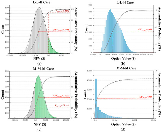
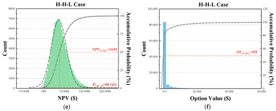
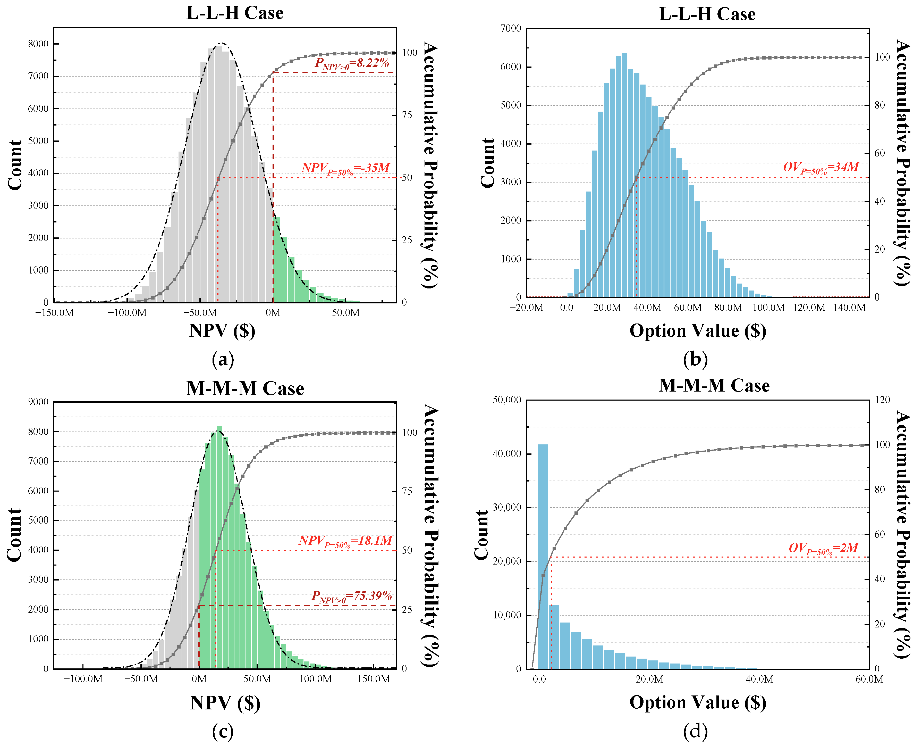
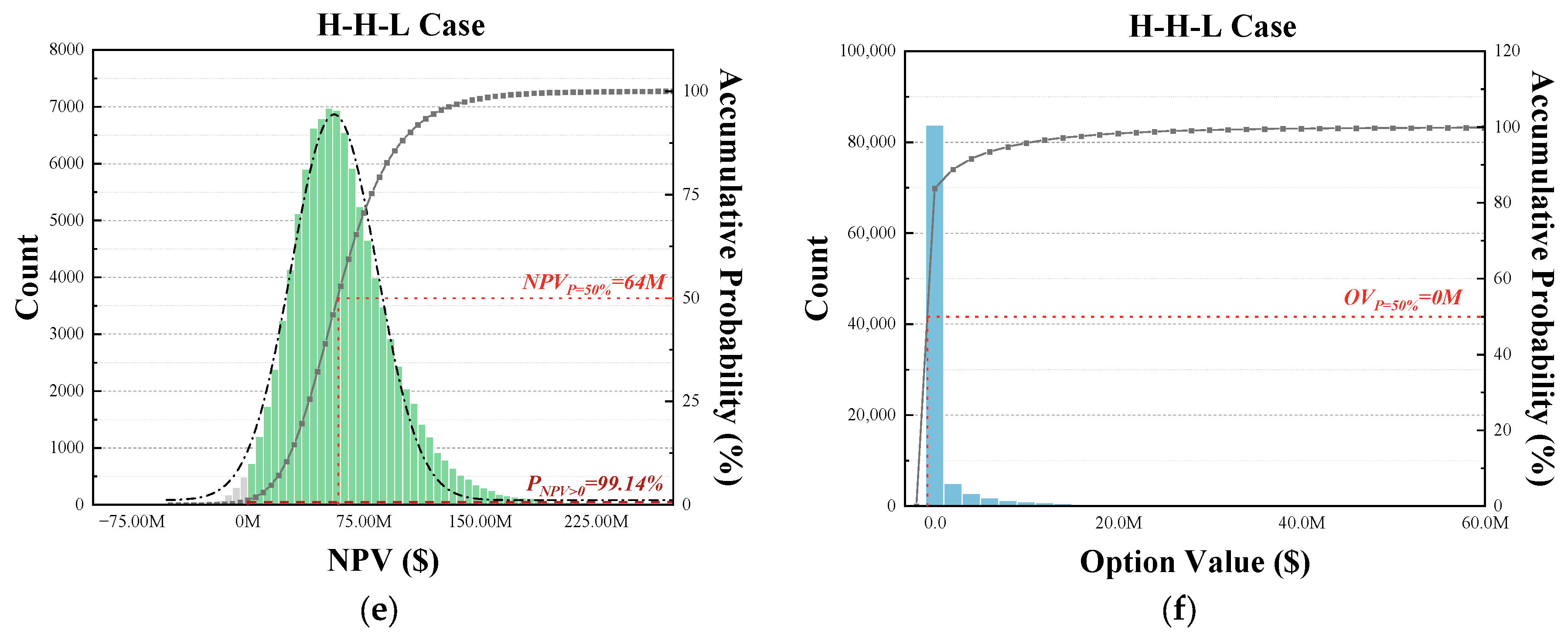
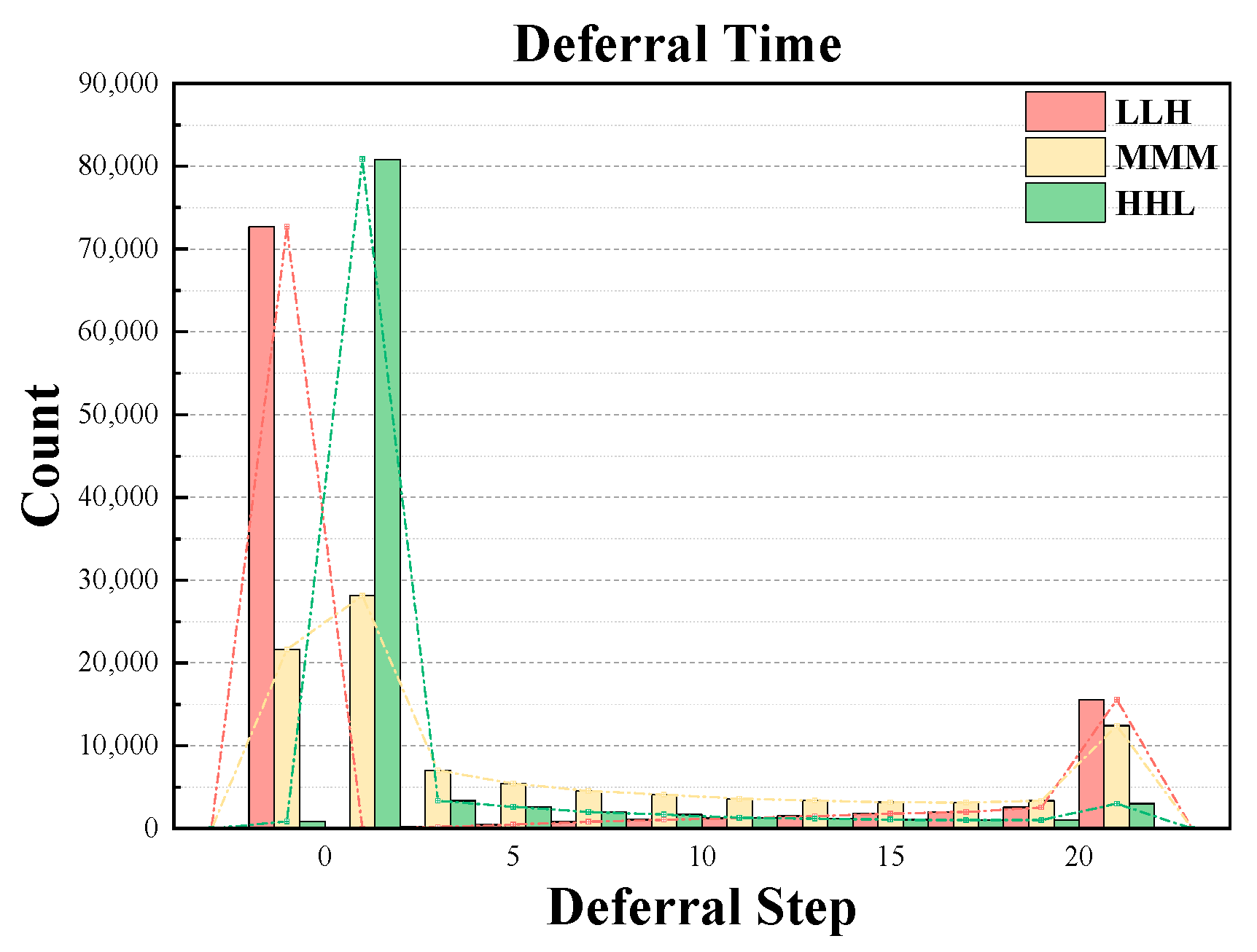
In addition, three typical scenarios, namely the worst LLH case, the middle MMM case, and the best HHL case, are chosen to graph the NPV and option value distribution, and the deferral time, as shown in Figure 8 and Figure 9.

Figure 8. NPV distribution of (a) L-L-H case; (c) M-M-M case; and (e) H-H-L case; option distribution of (b) L-L-H case; (d) M-M-M case; and (f) H-H-L case. The grey and green columns represent the loss and profit results, respectively, while the orange dotted lines and dark red lines indicate the mean NPV and profit likelihood. The blue columns and grey dot lines in the option plots represent the option value distribution and the accumulative probability, respectively.

Figure 9. Deferral time in three scenarios. The plot demonstrates the deferral time distribution of three typical scenarios. The red, yellow, and green dotted lines, respectively, indicate the trend of the optimal deferral time in the LLH, MMM, and HHL scenarios.

In the worst LLH situation, the NPV distribution is frequently located to the left of the zero axis, with a median of around USD −35M, and the likelihood of profit is only about 8%. This shows that the benchmark investment in this environment is loss-driven; only rare price rises can bring the project back on track. In addition, the medium option value is about USD 34M, showing that in over half of the paths, the ability to time investments or refrain from investing can yield an additional value at least 34M compared to immediate investment. The option value distribution is strictly positive and right-skewed long-tailed distribution, with the pronounced peak close to 30M. This indicates that the project flexibility is mainly achieved by avoiding the loss resulting from immediate investment, where the majority options involve not investing or postponing the decision making process. The long tail on the right side corresponds to a limited number of pathways that have capitalized on the rise in oil prices and ETA or the decline of CO₂ prices to capture a considerable upward gain when timing is appropriate. The deferral time is focused on −1 and 20, suggesting the options are either to refrain from investing entirely or to invest after five years.

In the middle MMM case, the NPV distribution is slightly right-skewed, with the 59.3% profit probability and the median USD 18.1M, which indicates that direct investment is acceptable within this market scenario. However, approximately 40% of the paths result in negative NPVs, indicating that the downside risks associated with oil prices and carbon costs cannot be disregarded. The option value with the median USD 2M exhibits a distribution resembling an L shape, characterized by a substantial quantity of samples near zero, indicating that immediate investment approaches the optimal condition, while deferring investment contributes minimal additional value. The immediate investment and never investing each account for more than 1/5, and median deferment time in the remaining paths is about 1.25 years, indicating that short-term investment waiting dominates.

The NPV distribution in the HHL scenario is significantly right-skewed, with profit probability approaching 100 and the median USD 64M. The corresponding option value is highly concentrated near zero and only has a small right tail, with median USD 0, indicating that in most cases the marginal value of waiting is small, and the current investment can already secure positive and stable economic returns, and the upward movement mainly comes from the sustained strength of the market rather than the choice of timing.

3.3. Global Sensitivity Analysis

All critical parameters involved in the project are categorized into three primary groups: economic, geological, and engineering parameters. The economic factors encompass market pricing connected to costs and revenues, as well as projected future earnings levels, which are subject to uncontrollable fluctuations, regarded as uncertain scenarios. The geological parameters, encompassing reservoir characteristics and oil quality, reflect the true geological circumstances of the project’s execution. These characteristics typically exist objectively and are mostly beyond control. The engineering parameters, encompassing the executed injection strategy and well engineering, are partially modifiable. Hence, this study employed a global sensitivity analysis suggested by ref. [31] under the static method, specifically the partial rank correlation coefficient, to identify which parameters significantly impact the project’s economics.

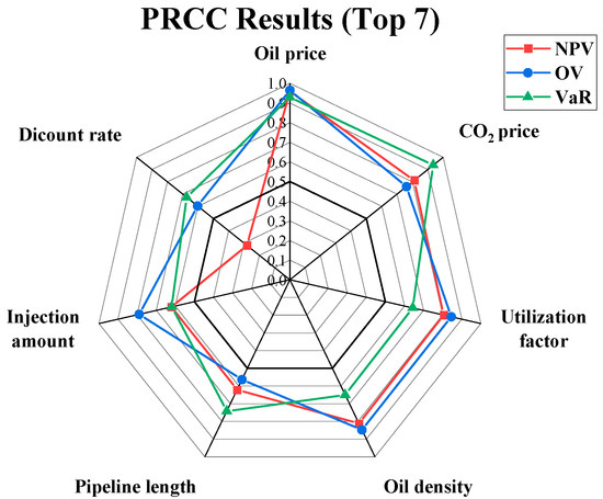
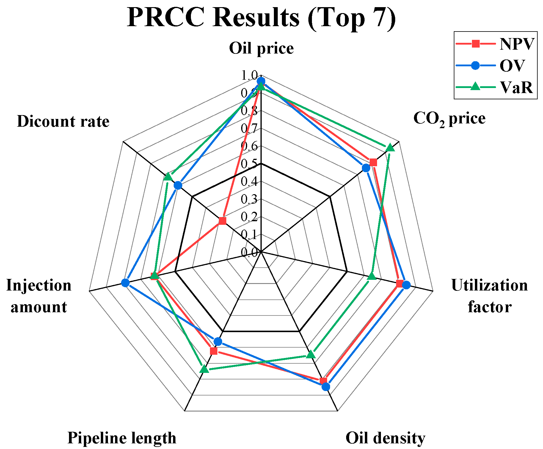
The Partial Rank Correlation Coefficient (PRCC) results in Table 8 and Figure 10 show that the uncertain scenarios involving the market series dominates the project economic, following by the objectively geological conditions and partially subjective engineering strategy. The oil price is the primary driving force, greatly enhancing returns and decreasing left-tail risks, while the CO₂ purchase price governs the left-tail risk, where an increase in the purchasing price leads to a substantial decline in NPVs accompanied with intolerable dangers. The oil density and utilization factor exhibit a similar effect to the final economic, wherein denser oil or oil with inferior gas driving effects will substantially inhibit yield. Furthermore, the volume of injection affects both advantages and hazards, as it enhances the average NPV in favorable market situations while amplifying risks in adverse market conditions. The pipe length, which solely influences costs, presents significant left-tail risks, suggesting that the project necessitates exceptionally stringent source–sink matching constraints. The other geological parameters including permeability, thickness, and the reservoir pressure, effects the economic viability of the project to a certain degree. Enhanced injection capability and thickness correlate with increased oil revenue, whereas elevated reservoir pressure necessitates higher initial pressure and diminishes injection capacity.

Table 8. PRCC results. The results illustrate the connection between NPV, OV, and value at risk (VaR) (with their ranks), along with the grouped parameters.

Group	Parameters	NPV/Rank	OV/Rank	VaR/Rank
Economic	Oil price	0.960/1	0.965/1	−0.929/2
	ETA	0.376/10	0.354/11	0.334/12
	CO2 price	−0.811/3	−0.761/5	−0.936/1
	Power price	−0.231/14	−0.192/17	−0.333/13
	Discount rate	−0.280/13	−0.603/6	0.674/4
Geological	Permeability	0.464/8	0.444/9	0.546/9
	Thickness	0.427/9	0.408/10	0.458/10
	Depth	−0.036/17	−0.031/15	0.040/18
	Reservoir pressure	−0.511/7	−0.477/8	−0.579/8
	Oil density	−0.812/2	−0.848/2	−0.650/5
	1st decline rate	−0.185/15	−0.222/14	−0.166/15
	2nd decline rate	−0.286/11	−0.316/12	−0.184/14
	Utilization factor	−0.805/4	−0.845/3	−0.643/6
Engineering	Duration	−0.053/16	−0.056/16	−0.072/16
	Slick water	−0.036/17	−0.018/18	−0.067/17
	Silica sand	0.023/19	0.008/19	−0.011/19
	Out pressure	0.288/12	0.269/13	0.340/11
	Injection amount	0.620/6	0.789/4	−0.619/7
	Pipeline length	−0.621/5	−0.564/7	−0.742/3

Figure 10. Radar plot of the PRCC results (top 7). The figure shows the absolute PRCC value of the top 7 chosen parameters.

In general, the two market series—oil price and CO₂ purchasing price—exert the most substantial influence on the NPV, PV, and VaR of the project compared to all other parameters. Meanwhile, factors such as pipe length, utilization factor, and oil density emerge as high-sensitivity elements that are partially controllable, ranking just below the market series in terms of impact. Moreover, the discount rate exhibits a notable sensitivity to the option value and the left tail, while the injection amount significantly impacts both profit and risk. Therefore, to achieve a superior mean NPV and mitigate left-tail risks, management should prioritize the establishment of a long-term contract for CO₂ procurement at a moderate and stable price, while also adjusting project injections in accordance with fluctuations in oil prices. Moreover, it is essential to execute a flexible engineering design of the source–sink pathway during the planning phase.

3.4. Economic Limit

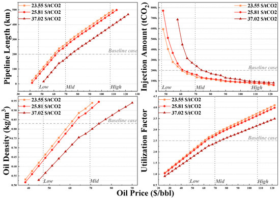
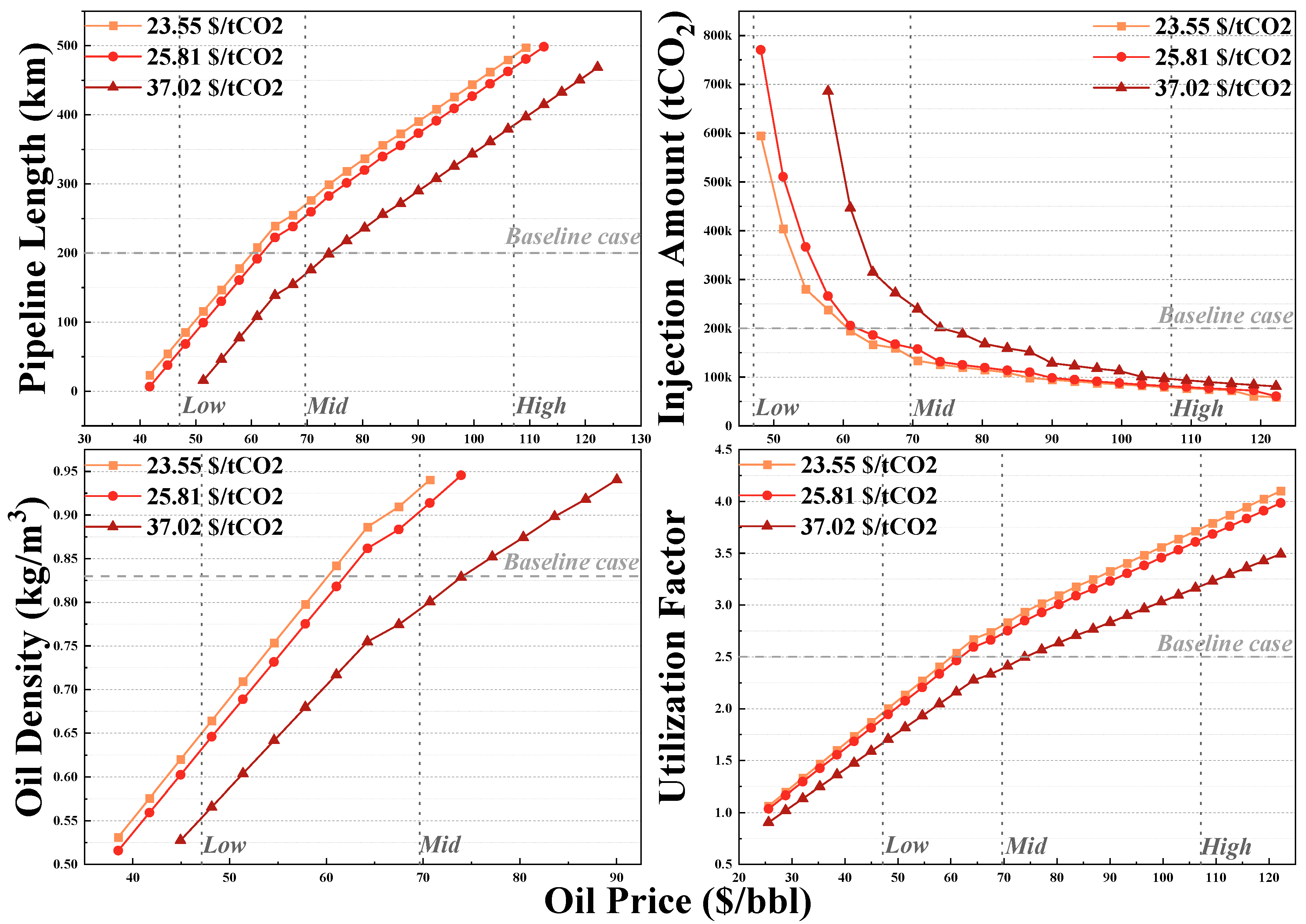
Based on the sensitivity results in the previous chapter, the controllable engineering parameters, namely pipeline length and injection amount, and the exogenous parameters that are difficult to change, namely the oil density and utilization factor, are chosen to construct the techno-economic limit evaluation. Based on the sensitivity results from the preceding chapter, the adjustable engineering parameters, namely pipeline length and injection volume, along with the exogenous parameters that are hard to modify, namely oil density and utilization factor, are selected to establish the evaluation of techno-economic limits. The approach involves graphing the curve of the chosen parameters at a zero NPV, with varying oil prices and three scenarios for CO₂ purchase prices, while keeping the other parameters in the basic line (median) value. The results depicted in Figure 11 indicate that oil prices and CO₂ purchase prices considerably influence the economic limits of four parameters. Owning to the special oil gains, the results demonstrate non-linearity and a threshold impact, where at lower oil price levels, the slope is steeper; however, at medium to high oil prices, it markedly flattens and enters a plateau phase.

Figure 11. Techno-economic limits results. The figure shows the economic limits of four selected parameters, namely pipeline length, injection amount, oil density, and utilization factor, at low, mid, and high CO₂ purchase price levels. The grey lines and dark grey dotted lines represent the values of each parameter in the baseline case and low, mid, and high oil price cases, respectively.

Within the mid oil price scenario, the economic limit of pipeline length reaches 175 km at high CO₂ price level, while it extends to 260 and 276 km at mid and high CO₂ price levels, respectively, surpassing the baseline case. This indicates that during the project design phase, if the project’s front end may choose the site, it serves as the most direct hard constraint to regulate the source–sink distance within economically viable bounds.

As the injection volume simultaneously boosts both the revenue side and the cost side, the margin profits brought by each volume of injected CO₂ increases with higher oil price. It is significant that the elasticity of the unit oil price relative to the scale threshold is markedly elevated in the low oil price range, with substantial economic injection scales, but the economic injection scales at varying CO₂ purchase price levels converge at elevated oil price levels. Moreover, at elevated CO₂ costs, there exists an unfeasible zone where the range below 58 USD/bbl is devoid of data, signifying that achieving break-even is unattainable at any size (100k–1M tons), and the 58 USD/bbl oil price is the market entry condition.

In a mid oil price scenario, the economic thresholds for oil density are 0.94, 0.91, and 0.80 kg/m³ for low, mid, and high CO₂ purchase price levels, respectively, while the economic thresholds for utilization factor are 2.8, 2.7, and 2.4 at the same CO₂ purchase price levels. This suggests that light oil is also vital in scenarios of low oil prices, and it is necessary to reduce the injection–production ratio through techniques such as displacement schemes and well pattern optimization.

Therefore, the techno-economic threshold at a net present value of zero delineates the viable boundaries of four essential engineering and geological parameters, considering varying oil prices and CO₂ acquisition costs, thereby establishing the permissible range of critical parameters for subsequent project planning and execution.

4. Conclusions

This study, grounded on a real CCUS-EOR project, has developed a comprehensive assessment framework encompassing market, engineering, and financial dimensions. Specifically, utilizing historical market data, the scenarios in both static and dynamic states, derived from Markov stochastic market paths, are integrated with the simulated costs and production data from the project, subsequently assessing the project’s economic performance via the deferral option. In addition, the PRCC approach is employed for global sensitivity analysis to identify significant drivers, therefore delineating the value and feasibility domains of certain parameters. Based on systematic evidence, the following findings have been reached:

The oil price and CO₂ price are essential factors that influence the cash flow differential and distribution of the NPV and option value, with the marginal effect of oil price being affected by specific oil gains and injection scale, exhibiting a non-linear pattern. Currently, the ETA prices in the Chinese market little affect the project’s profitability and do not influence cash flow to the same extent as oil and CO₂ pricing. Within the scenarios of CO₂ prices ranging from low to high, the proposed entry oil prices at which the project may avoid losses are 66.5, 68.5, and 81.6 USD/bbl, respectively, while the earnings from the ETA can mitigate up to 5 USD/bbl of oil prices. In addition, in the most adverse market conditions, postponing the start of construction can substantially enhance the expected value and mitigate the risk in the left tail. This indicates that the unfeasible static situation acquires positive potential under dynamic timing, demonstrating the value of management flexibility. This state-dependent outcome offers a practical timing implication: when simulated market trajectories persist in low-oil or high-CO₂ cost environments, the value of the deferral option escalates, favoring a “wait” decision; conversely, transitions into sustained favorable conditions advocate for earlier investment. Furthermore, the primary factors influencing project profitability are oil prices and CO₂ prices, which are unpredictable market variables. The third and fourth characteristics of considerable impact are the utilization factor and the oil density associated with the oil product, with the former being controllable via the injection process. The fifth component is the pipeline length, indicating the importance of source–sink alignment, while the sixth factor is the injection volume, demonstrating that in a moderate market, scale effects enhance profitability. From an engineering design standpoint, pipeline length serves as an indicator for CO₂ source–sink alignment, while injection volume suggests that the selection of injection scale should correspond with existing market conditions and established feasibility parameters, rather than being predetermined. The techno-economic constraints are subsequently established for project completion, illustrating the thresholds of four parameters associated with engineering and geology under varying market conditions of oil and CO₂ prices.

Consequently, it is advisable for management to continuously monitor oil and CO₂ prices, stabilize cash flow through long-term CO₂ purchasing agreements, and retain the flexibility to defer initiation or diminish size under unfavorable market conditions. As the Chinese carbon trading system evolves and the ETA is expected to increase, commencing or extending projects at this juncture can capitalize on the elevated and more predictable revenue from ETA to mitigate negative impacts. In the engineering domain, during the project initiation and ongoing assessment phases, the project team must prioritize the integration of source–sink configurations, the optimization of well patterns and injection strategies, and the enhancement of CO₂ injection efficiency, as these elements are primary management decision variables. From the government’s institutional perspective, it is essential to enhance the risk-adjusted returns of high-quality projects and direct limited public funds and carbon resources towards initiatives that exhibit optimal source–sink alignment, suitable physical characteristics, high utilization rates, and substantial economies of scale.

The limitation of this analysis is that it does not include composite options such as abandonment or expansion, and the combination of full physical reservoir and regional price is yet to be introduced. Consequently, future study will encompass multi-period expansion or contraction decisions, as well as geological and production joint sampling, to further improve guidance capabilities. In conclusion, this study offers a solid techno-economic evaluation model and decision-making framework for CCUS-EOR projects, establishing a robust foundation for project decisions and future policy development.

Appendix A.1. Compression and Pumping

The study has applied 5-stage compressor combined with a pump to compress CO₂ from atmosphere to the wellhead pressure. The following equations illustrate the power necessary for compression and pumping. Subsequently, the required number of compressors can be determined by dividing the maximum power demand by the rated power of an individual compressor, which is set at 3000 kW.

$$W_i^{com}={\displaystyle \sum _{j=1}^{N_s}\frac{5Q_i^d{Z}_{s,j}R{T}_{in}{K}_{s,j}}{432M{\eta }_{com}(K_{s,j}-1)}[{(\frac{P_{cut,j}}{P_{initial,j}})}^{\frac{K_{s,j}-1}{N_s{K}_{s,j}}}-1]}$$

(A1)

$$W_i^{pump}={\displaystyle \frac{625Q_i^d(P_{out}-P_{cut})}{54{\rho }_{pump}{\eta }_{pump}}}$$

(A2)

$$n_{i,train}={\displaystyle \frac{W_i^{com}}{30000}}$$

(A3)

$$Q_i^d={\displaystyle \frac{Q_i^{car}}{365{\eta }_{well}}}$$

(A4)

where N_s denotes the stage number, valuing at 5 in this study, and the other values can be assumed: R = 8.314 J/mol·K; M = 44.01 g/mol; ρ_pump is the CO₂ density during pumping deduced according to Appendix A.3; $Q_i^d$ represents the daily injection volume; and η_well denotes the efficiency of the injection well, established at 0.82.

Table A1. Thermodynamic parameters in segmented compression [32]. The table demonstrates the pressure, temperature, and specific heat ratio and compressibility of CO₂ in each stage.

Parameter	Symbol	Stage 1	Stage 2	Stage 3	Stage 4	Stage 5
Pressure (MPa)	Pinitial–Pcut	0.1–0.24	0.24–0.56	0.56–1.32	1.32–3.12	3.12–7.38
Temperature (K)	Tin	353	353	353	353	353
Specific heat ratio	Ks,j	1.274	1.285	1.313	1.396	1.742
Compressibility	Zs,j	1.003	0.993	0.978	0.943	0.852

Table A1. Thermodynamic parameters in segmented compression [32]. The table demonstrates the pressure, temperature, and specific heat ratio and compressibility of CO₂ in each stage.

Parameter	Symbol	Stage 1	Stage 2	Stage 3	Stage 4	Stage 5
Pressure (MPa)	Pinitial–Pcut	0.1–0.24	0.24–0.56	0.56–1.32	1.32–3.12	3.12–7.38
Temperature (K)	Tin	353	353	353	353	353
Specific heat ratio	Ks,j	1.274	1.285	1.313	1.396	1.742
Compressibility	Zs,j	1.003	0.993	0.978	0.943	0.852

Appendix A.2. Maximum Injection Rate and Well Number

To prevent gas surging, the maximum daily CO₂ injection rate of a single well can be obtained via the following formula:

$$Q_{well}=0.0208{\displaystyle \frac{\sqrt{0.3k_h^2}}{{\mu }_{in}}}h(P_{down}-P_{res})$$

(A5)

where μ_in represents the viscosity of CO₂ at intermediate pressure and temperature, which are calculated in Appendix A.3; P_down denotes down-hole pressure.

In Equation (A5), the down-hole pressure is determined through an iterative process, calculated by adding the wellhead pressure to the gravity head and then subtracting the frictional pressure loss in the injection pipe.

$$P_{down}=P_{out}+{\displaystyle \frac{{\rho }_{mid}gd}{{10}^6}}-\Delta P_{pipe}$$

(A6)

$$F_f={\displaystyle \frac{1}{4\cdot {\{-1.8\ln [\frac{149.26{\mu }_{mid}{D}_{pipe}}{Q_{well}}+{(\frac{0.3048\epsilon }{3.7D_{pipe}})}^{1.11}]\}}^2}}$$

(A7)

$$v_{mid}={\displaystyle \frac{5Q_{well}}{108{\rho }_{mid}\pi {D_{pipe}}^2}}$$

(A8)

$$\Delta P_{pipe}={\displaystyle \frac{{\rho }_{mid}{F}_{f}d{v_{mid}}^2}{2\cdot {10}^6{D}_{pipe}}}$$

(A9)

where ρ_mid and μ_mid represent the CO₂ density and viscosity during injection, which are calculated in Appendix A.3; v_mid and F_f denotes the velocity during injection and the fanning friction factor, respectively; D_pipe is the diameter of an injection pipe, established at 0.06 m, while ε signifies injection pipe roughness factor, determined as 0.00015 ft.

In the first iteration, the down-hole pressure is established at 22 MPa, and the iteration concludes when the error between iterations falls below 0.1%. Therefore, after verifying the actual down-hole pressure, the maximum injection rate may be determined, leading to the calculation of the required number of injection wells based on the annual injection volume:

$$N_i^{inj}=Round\_up({\displaystyle \frac{Q_i^d}{Q_{well}}})$$

(A10)

Appendix A.3. Correlation of CO₂ Density and Viscosity

Variations in injection depth result in fluctuations in pressure and temperature within the pipe, therefore altering the actual density and viscosity of the injected CO₂ during the injection process. Therefore, for the sake of simplicity in calculations, the study has assumed that the density and viscosity of CO₂ remain constant at mid-range temperature and pressure values during injection.

$$T_{mid}=(T_{in}+T_{sur}+T_{g}d)/2$$

(A11)

$$T_{inter}=(T_{res}+T_{sur}+T_{g}d)/2$$

(A12)

$$P_{mid}=(P_{out}+P_{down})/2$$

(A13)

$$P_{inter}=(P_{down}+P_{res})/2$$

(A14)

where T_sur represents the surface temperature of 294.5 K; T_g is the geothermal gradient, valuing at 0.021 K/m; T_res denotes the reservoir temperature at 345 K.

The regression equations are employed to deduce the density and viscosity of CO₂ during both the injection and intermediate stages.

$$\rho (T,P)=A_T{P}^6+B_T{P}^5+C_T{P}^4+D_T{P}^3+E_T{P}^2+F_T{P}^1+G_T{P}^0$$

(A15)

$$\mu (T,P)=a_T{P}^6+b_T{P}^5+c_T{P}^4+d_T{P}^3+e_T{P}^2+f_T{P}^1+g_T{P}^0$$

(A16)

where the coefficients for CO₂ density and viscosity belong to the coefficient sets {A, B, C, D, E, F, G}_T and {a, b, c, d, e, f, g}_T, which correspond to a specific temperature shown in Table A2 and Table A3.

Table A2. Regression equation coefficients for CO₂ density.

Temperature (K)	A (P6)	B (P5)	C (P4)	D (P3)	E (P2)	F (P1)	G (P0)
310.8	−5.43 × 10−4	5.98 × 10−2	−2.71 × 10	6.45 × 101	−8.51 × 102	5.93 × 103	−1.63 × 104
316.3	9.61 × 10−4	−9.44 × 10−2	3.73 × 10	−7.54 × 101	8.08 × 102	−4.21 × 103	8.42 × 103
321.9	1.03 × 10−3	−1.05 × 10−1	4.36 × 10	−9.33 × 101	1.08 × 103	−6.23 × 103	1.43 × 104
327.4	4.92 × 10−4	−5.31 × 10−2	2.33 × 10	−5.29 × 101	6.49 × 102	−3.97 × 103	9.61 × 103
333.0	1.78 × 10−5	−5.26 × 10−3	3.80 × 10−1	−1.20 × 101	1.86 × 102	−1.32 × 103	3.61 × 103
338.6	−2.01 × 10−4	1.79 × 10−2	−6.14 × 10−1	9.95 × 10	−7.50 × 101	2.48 × 102	−1.21 × 102
344.1	−2.27 × 10−4	2.18 × 10−2	−8.26 × 10−1	1.56 × 101	−1.54 × 102	7.79 × 102	−1.49 × 103
349.7	−1.72 × 10−4	1.71 × 10−2	−6.76 × 10−1	1.34 × 101	−1.40 × 102	7.58 × 102	−1.56 × 103
355.8	−1.04 × 10−4	1.07 × 10−2	−4.39 × 10−1	9.02 × 10	−9.70 × 101	5.47 × 102	−1.16 × 103

Table A2. Regression equation coefficients for CO₂ density.

Temperature (K)	A (P6)	B (P5)	C (P4)	D (P3)	E (P2)	F (P1)	G (P0)
310.8	−5.43 × 10−4	5.98 × 10−2	−2.71 × 10	6.45 × 101	−8.51 × 102	5.93 × 103	−1.63 × 104
316.3	9.61 × 10−4	−9.44 × 10−2	3.73 × 10	−7.54 × 101	8.08 × 102	−4.21 × 103	8.42 × 103
321.9	1.03 × 10−3	−1.05 × 10−1	4.36 × 10	−9.33 × 101	1.08 × 103	−6.23 × 103	1.43 × 104
327.4	4.92 × 10−4	−5.31 × 10−2	2.33 × 10	−5.29 × 101	6.49 × 102	−3.97 × 103	9.61 × 103
333.0	1.78 × 10−5	−5.26 × 10−3	3.80 × 10−1	−1.20 × 101	1.86 × 102	−1.32 × 103	3.61 × 103
338.6	−2.01 × 10−4	1.79 × 10−2	−6.14 × 10−1	9.95 × 10	−7.50 × 101	2.48 × 102	−1.21 × 102
344.1	−2.27 × 10−4	2.18 × 10−2	−8.26 × 10−1	1.56 × 101	−1.54 × 102	7.79 × 102	−1.49 × 103
349.7	−1.72 × 10−4	1.71 × 10−2	−6.76 × 10−1	1.34 × 101	−1.40 × 102	7.58 × 102	−1.56 × 103
355.8	−1.04 × 10−4	1.07 × 10−2	−4.39 × 10−1	9.02 × 10	−9.70 × 101	5.47 × 102	−1.16 × 103

Table A3. Regression equation coefficients for CO₂ viscosity.

Temperature (K)	A (P6)	B (P5)	C (P4)	D (P3)	E (P2)	F (P1)	G (P0)
310.8	9.45 × 10−11	−9.37 × 10−9	3.75 × 10−7	−7.70 × 10−6	8.44 × 10−5	−4.58 × 10−4	9.69 × 10−4
316.3	4.61 × 10−11	−4.65 × 10−9	1.89 × 10−7	−3.98 × 10−6	4.50 × 10−5	−2.50 × 10−4	5.51 × 10−4
321.9	2.17 × 10−11	−2.27 × 10−9	9.72 × 10−8	−2.17 × 10−6	2.62 × 10−5	−1.57 × 10−4	3.81 × 10−4
327.4	1.75 × 10−11	−1.84 × 10−9	7.91 × 10−8	−1.78 × 10−6	2.18 × 10−5	−1.33 × 10−4	3.32 × 10−4
333.0	1.59 × 10−11	−1.66 × 10−9	7.09 × 10−8	−1.58 × 10−6	1.93 × 10−5	−1.18 × 10−4	2.99 × 10−4
338.6	1.33 × 10−11	−1.38 × 10−9	5.86 × 10−8	−1.30 × 10−6	1.59 × 10−5	−9.75 × 10−5	2.52 × 10−4
344.1	9.60 × 10−12	−9.95 × 10−10	4.21 × 10−8	−9.35 × 10−7	1.15 × 10−5	−7.10 × 10−5	1.90 × 10−4
349.7	4.94 × 10−12	−5.14 × 10−10	2.19 × 10−8	−4.94 × 10−7	6.23 × 10−6	−3.93 × 10−5	1.15 × 10−4
355.8	8.35 × 10−13	−9.24 × 10−11	4.29 × 10−9	−1.10 × 10−7	1.66 × 10−6	−1.17 × 10−5	4.94 × 10−5

Table A3. Regression equation coefficients for CO₂ viscosity.

Temperature (K)	A (P6)	B (P5)	C (P4)	D (P3)	E (P2)	F (P1)	G (P0)
310.8	9.45 × 10−11	−9.37 × 10−9	3.75 × 10−7	−7.70 × 10−6	8.44 × 10−5	−4.58 × 10−4	9.69 × 10−4
316.3	4.61 × 10−11	−4.65 × 10−9	1.89 × 10−7	−3.98 × 10−6	4.50 × 10−5	−2.50 × 10−4	5.51 × 10−4
321.9	2.17 × 10−11	−2.27 × 10−9	9.72 × 10−8	−2.17 × 10−6	2.62 × 10−5	−1.57 × 10−4	3.81 × 10−4
327.4	1.75 × 10−11	−1.84 × 10−9	7.91 × 10−8	−1.78 × 10−6	2.18 × 10−5	−1.33 × 10−4	3.32 × 10−4
333.0	1.59 × 10−11	−1.66 × 10−9	7.09 × 10−8	−1.58 × 10−6	1.93 × 10−5	−1.18 × 10−4	2.99 × 10−4
338.6	1.33 × 10−11	−1.38 × 10−9	5.86 × 10−8	−1.30 × 10−6	1.59 × 10−5	−9.75 × 10−5	2.52 × 10−4
344.1	9.60 × 10−12	−9.95 × 10−10	4.21 × 10−8	−9.35 × 10−7	1.15 × 10−5	−7.10 × 10−5	1.90 × 10−4
349.7	4.94 × 10−12	−5.14 × 10−10	2.19 × 10−8	−4.94 × 10−7	6.23 × 10−6	−3.93 × 10−5	1.15 × 10−4
355.8	8.35 × 10−13	−9.24 × 10−11	4.29 × 10−9	−1.10 × 10−7	1.66 × 10−6	−1.17 × 10−5	4.94 × 10−5

Appendix B.1. Costs Within Transport Stage

Detailed formulas for CAPEX and O&M costs in the carbon dioxide transportation stage.

$$CAPE{X}_i^{pipeline}=79023L$$

(A17)

$$CAPE{X}_i^{com+pump}=3.57{(Q_i^{car})}^{0.29}+190.95{(Q_i^{car})}^{0.4}+962.36W_i^{pump}+60689.24$$

(A18)

$$O\&M_i^{pipeline}=3807L+0.03Q_i^{car}L$$

(A19)

$$O\&M_i^{com+pump}=0.04CAPE{X}_i^{com+pump}$$

(A20)

$$O\&M_i^{elec}=S_i^p\cdot 365\cdot 24\cdot (\eta W_i^{com}+W_i^{pump})$$

(A21)

where L represents the pipeline length; $W_i^{com}$ and $W_i^{pump}$ denote the power consumption of compressors and pumps in the ith year; $S_i^p$ represents the power price in the year i. η_com and η_pump denote the efficiencies of compressor and pump, setting at 0.75.

Appendix B.2. Costs Within Utilization and Storage Stage

Detailed formulas for CAPEX and O&M costs in the Carbon Dioxide Utilization and Storage Stage.

$$CAPE{X}_i^{ge}=26.1N_i^{well}$$

(A22)

$$N_i^{well}=N_i^{inj}+N_i^{pro}$$

(A23)

$$N_i^{pro}=\delta N_i^{inj}$$

(A24)

$$O\&M_i^{surface}=13368N_i^{well}{({\displaystyle \frac{Q_i^d}{280}})}^{0.5}$$

(A25)

$$O\&M_i^{subsurface}=4914N_i^{well}({\displaystyle \frac{d}{1219}})$$

(A26)

$$O\&M_i^{others}=24181N_i^{well}$$

(A27)

$$O\&M_i^{monitor}=0.1Q_i^{car}$$

(A28)

where $N_i^{inj}$ and $N_i^{pro}$ represent the number of injection wells and production wells required in year i; δ represents the injection–production well ratio, valuing at 2.4.

References

- International Energy Agency (IEA). CCUS Projects Around the World Are Reaching New Milestones. 2025. Available online: https://www.iea.org/commentaries/ccus-projects-around-the-world-are-reaching-new-milestones (accessed on 30 April 2025).
- Cao, C.; Zhu, H.; Hou, Z. Advances in Carbon Capture, Utilization and Storage (CCUS). Energies 2024, 17, 4784. [Google Scholar] [CrossRef] [Scilit]
- Zhang, Y.-Q.; Yang, S.-L.; Bi, L.-F.; Gao, X.-Y.; Shen, B.; Hu, J.-T.; Luo, Y.; Zhao, Y.; Chen, H.; Li, J. A Technical Review of CO2 Flooding Sweep-Characteristics Research Advance and Sweep-Extend Technology. Pet Sci. 2025, 22, 255–276. [Google Scholar] [CrossRef] [Scilit]
- Liu, X.; Chen, H.; Li, Y.; Zhu, Y.; Liao, H.; Zhao, Q.; Zhou, X.; Zeng, H. Oil Production Characteristics and CO2 Storage Mechanisms of CO2 Flooding in Ultra-Low Permeability Sandstone Oil Reservoirs. Pet. Explor. Dev. 2025, 52, 196–207. [Google Scholar] [CrossRef] [Scilit]
- Zang, X.; Bian, J.; Ni, Y.; Zheng, W.; Zhu, T.; Chen, Z.; Cao, X.; Huang, J.; Lai, Y.; Lin, Z. A Robust Biomimetic Superhydrophobic Coating with Superior Mechanical Durability and Chemical Stability for Inner Pipeline Protection. Adv. Sci. 2024, 11, 2305839. [Google Scholar] [CrossRef] [Scilit] [PubMed]
- Gholami, R.; Raza, A.; Iglauer, S. Leakage Risk Assessment of a CO2 Storage Site: A Review. Earth-Sci. Rev. 2021, 223, 103849. [Google Scholar] [CrossRef] [Scilit]
- Han, Z.; Liu, H.; Zhao, D.; Chen, Y.; Xing, Y.; Zhang, Z. Monte Carlo Sensitivity Analysis for a Carbon Capture, Utilization, and Storage Whole-Process System. Processes 2025, 13, 1356. [Google Scholar] [CrossRef] [Scilit]
- Wu, Q.; Li, Y.; Lin, Q.; Xu, D. Development of a Techno-Economic Assessment Model for Optimal Timing of CCUS Deployment Based on Compound Climate Change Mitigation Value. J. Clean. Prod. 2025, 516, 145760. [Google Scholar] [CrossRef] [Scilit]
- Obi, D.; Onyekuru, S.; Orga, A. Minimizing Carbon Capture Costs in Power Plants: A Dimensional Analysis Framework for Optimizing Hybrid Post-Combustion Systems. Energy Sci. Eng. 2025, 13, 2247–2261. [Google Scholar] [CrossRef] [Scilit]
- Nikravesh, H.; Ranjbar, A.; Azin, R. Optimizing the Wells Location Using the Metaheuristic Algorithms, as Well as Optimizing the Drilling Time of Production and Injection Wells in One of the Reservoirs in South West of Iran. Earth Sci. Inform. 2023, 17, 1393–1410. [Google Scholar] [CrossRef] [Scilit]
- International Monetary Fund (IMF). Global Price of Brent Crude [POILBREUSDM]. FRED, Federal Reserve Bank of St. Louis. 2025. Available online: https://fred.stlouisfed.org/series/POILBREUSDM (accessed on 21 August 2025).
- International Monetary Fund (IMF). Global Price of Dubai Crude [POILDUBUSDM]. FRED, Federal Reserve Bank of St. Louis. 2025. Available online: https://fred.stlouisfed.org/series/POILDUBUSDM (accessed on 21 August 2025).
- Federal Reserve Bank of St. Louis (FRED). Spot Crude Oil Price: West Texas Intermediate (WTI) [WTISPLC]. 2025. Available online: https://fred.stlouisfed.org/series/WTISPLC (accessed on 21 August 2025).
- Beijing Carbon Emission Rights Electronic Trading Platform. Trading Information of Beijing Carbon Emission Rights Electronic Trading Platform. 2025. Available online: https://www.bjets.com.cn/article/jyxx/ (accessed on 21 August 2025).
- Chongqing Public Resources Trading Center. Chongqing Carbon Emission Rights Trading Transaction Information. 2025. Available online: https://www.cqggzy.com/xxhz/014006/014006004/transaction_detail.html (accessed on 21 August 2025).
- Guangzhou Emission Exchange. Carbon Emission Market Quotation Information. 2025. Available online: https://www.cnemission.com/cpfw/jypt/lshqing/ (accessed on 21 August 2025).
- Hubei Carbon Emission Exchange. Carbon Emission Rights Trading Data [HBEA]. 2025. Available online: https://www.hbets.cn/list_30.html (accessed on 21 August 2025).
- Shenzhen Green Exchange. Trading Data and Information [SZEA]. 2025. Available online: https://szets.com/jysj.html (accessed on 21 August 2025).
- China National Emission Exchange. Daily Comprehensive Price Quotes and Transaction Information of the National Carbon Market. 2025. Available online: https://www.cneeex.com/qgtpfqjy/mrgk/2025n/index.shtml (accessed on 21 August 2025).
- U.S. Bureau of Labor Statistics (BLS). Producer Price Index by Industry: Industrial Gas Manufacturing: Carbon Dioxide [PCU3251203251204]. FRED, Federal Reserve Bank of St. Louis. 2025. Available online: https://fred.stlouisfed.org/series/PCU3251203251204 (accessed on 21 August 2025).
- SCI99 Inc. Monthly Carbon Dioxide Price. 2025. Available online: https://intl.sci99.com/ (accessed on 21 August 2025).
- McCoy, S.T. The Economics of CO2 Transport by Pipeline and Storage in Saline Aquifers and Oil Reservoirs. Doctoral Dissertation, Carnegie Mellon University, Pittsburgh, PA, USA, 2008. Available online: https://www.cmu.edu/ceic/assets/docs/publications/phd-dissertations/2008/sean-mccoy-phd-thesis-2008.pdf (accessed on 21 August 2025).
- Liu, B. Economic Evaluation Technology and Development Direction of CCUS-EOR Project. Pet. Sci. Technol. Forum 2023, 42, 57–66. (In Chinese) [Google Scholar] [CrossRef]
- McCollum, D.L.; Ogden, J.M. Techno-Economic Models for Carbon Dioxide Compression, Transport, and Storage & Correlations for Estimating Carbon Dioxide Density and Viscosity [Research Report]; Institute of Transportation Studies, University of California: Davis, CA, USA, 2006. [Google Scholar]
- Wei, N.; Li, X.; Dahowski, R.T.; Davidson, C.L.; Liu, S.; Zha, Y. Economic Evaluation on CO2-EOR of Onshore Oil Fields in China. Int. J. Greenh. Gas Control 2015, 37, 170–181. [Google Scholar] [CrossRef] [Scilit]
- Dutta, R.; Kundu, G.; Mousavi Mirkalaei, S.M.; Chakraborty, R.; Yomdo, S.; Mandal, A. Evaluation of Potential of CO2-Enhanced Oil Recovery (EOR) and Assessment of Capacity for Geological Storage in a Mature Oil Reservoir within Upper Assam Basin, India. Energy Fuels 2024, 38, 14096–14118. [Google Scholar] [CrossRef] [Scilit]
- Sun, H.; Wang, H.; Wu, G.; Wang, Y. CO2 EOR Factors in Heavy Oil Reservoirs. Pet. Geol. Exp. 2020, 42, 1009–1013+1023. (In Chinese) [Google Scholar] [CrossRef]
- Yang, Y. Research and Application of CO2 Flooding Technology in Extra-low Permeability Reservoirs of Shengli Oilfield. Pet. Geol. Recovery Effic. 2020, 27, 11–19. (In Chinese) [Google Scholar] [CrossRef]
- Mehrdoust, F.; Noorani, I.; Kanniainen, J. Valuation of Option Price in Commodity Markets Described by a Markov-Switching Model: A Case Study of WTI Crude Oil Market. Math. Comput. Simul. 2023, 215, 228–269. [Google Scholar] [CrossRef] [Scilit]
- Lin, B.; Tan, Z. How Much Impact Will Low Oil Price and Carbon Trading Mechanism Have on the Value of Carbon Capture Utilization and Storage (CCUS) Project? Analysis Based on Real Option Method. J. Clean. Prod. 2021, 298, 126768. [Google Scholar] [CrossRef] [Scilit]
- Wang, W.; Wang, X. An Efficient Variance-Based Global Sensitivity Index Based on C-DRM and Taylor Expansion. Proceedings of the Institution of Mechanical Engineers. Part E J. Process Mech. Eng. 2020, 235, 887–898. [Google Scholar] [CrossRef] [Scilit]
- National Institute of Standards and Technology (NIST), Office of Data and Informatics. Isothermal Properties for Water [Online Tool/Database]; National Institute of Standards and Technology (NIST): Gaithersburg, MD, USA, 2025. [Google Scholar]
Disclaimer/Publisher’s Note: The statements, opinions and data contained in all publications are solely those of the individual author(s) and contributor(s) and not of MDPI and/or the editor(s). MDPI and/or the editor(s) disclaim responsibility for any injury to people or property resulting from any ideas, methods, instructions or products referred to in the content. |
© 2026 by the authors. Licensee MDPI, Basel, Switzerland. This article is an open access article distributed under the terms and conditions of the Creative Commons Attribution (CC BY) license.