


Abstract
Understanding ecosystem recovery following flood events is critical for sustainable floodplain management, yet causal evidence linking flooding to vegetation recovery remains limited. This study investigated the causal impact of the 2022 flood on ecosystem recovery in the Chi River Basin, Thailand, using 232,172 spatial points with multi-temporal VCI data (2020–2024). We employed Propensity Score Matching (PSM) to control for confounding factors and Difference-in-Differences (DiD) to estimate the causal effect. XGBoost with SHAP analysis identified predictors of Slow Recovery Hotspots, and a four-tier policy zoning framework was developed for sustainable land use planning. The DiD estimate of −0.0734 (95% CI: −0.0802, −0.0666) in standardized VCI units (equivalent to a raw VCI reduction of 2.47 units on the 0–100 scale) suggests that flooding caused a significant reduction in vegetation recovery, with effects persisting for at least two years. Slow Recovery Hotspots—defined as locations where two-year post-flood VCI remained below pre-flood levels—comprised 51.1% of the study area (118,643 points), with estimated annual economic losses of 226.2 Million Baht (95% CI: 203.6–248.8 Million Baht). SHAP analysis revealed that pre-flood VCI (48.6%), elevation (21.6%), and pre-flood NDVI (13.5%) were the dominant predictors. A critical elevation threshold of 145–155 m was identified, with flood frequency showing cumulative effects (≥2 events out of 5 observation years significantly increasing risk). A four-tier policy zoning framework (Red: 4.5%, Yellow: 46.6%, Orange: 10.0%, Green: 38.9%) was developed, providing actionable recommendations including no-build zones, land buyouts, building codes, early warning systems, and drainage improvements. Scenario-based analysis suggests that implementation could reduce economic losses by 30–40% (67.9–90.5 Million Baht/year). The approach demonstrates the value of combining causal inference with machine learning for evidence-based floodplain management. This framework contributes to SDGs 2, 6, 11, 13, and 15 and is transferable to other flood-prone regions in Southeast Asia.
1. Introduction
1.1. The Challenge of Flood Hazard Assessment in Low-Gradient Floodplains
Flooding is among the most frequent and economically damaging natural hazards globally, with annual losses exceeding USD 50 billion and affecting over 250 million people annually [1]. Southeast Asia bears a disproportionate share of this burden due to its dense river networks, monsoonal climate, and rapidly expanding urban footprints [2]. Thailand’s 2011 floods exemplified this vulnerability, affecting 13 million people and causing estimated economic damages of USD 46.5 billion [3]. In northeastern Thailand’s Chi River Basin, seasonal inundation recurs with such regularity that residents have adapted their livelihoods around flood pulses, yet severe events continue to disrupt lives and infrastructure [4].
The Chi River Basin exemplifies a paradox common to many tropical floodplain environments: despite being a low-lying floodplain, the region experiences both severe seasonal flooding and recurrent agricultural drought [5,6,7,8]. This “floodplain–drought paradox” is driven by three interacting factors: (1) sandy soils of the Khorat Plateau with extremely low water-holding capacity (50–80 mm/m) that drain rapidly after inundation; (2) deep incision of the Chi River main channel (5–10 m below the floodplain), limiting irrigation access even from locations within 500 m of the river; and (3) pronounced seasonal rainfall variability with a distinct dry season (November–April) and frequent dry spells during the wet season [9,10,11]. Compound drought–flood events have been increasingly documented globally, with lagged compound occurrences of droughts and pluvials observed over the past seven decades [12]. These characteristics make the Chi River Basin an ideal natural laboratory for studying the relationships between topography, flood dynamics, and ecosystem recovery.
Effective flood risk management requires reliable predictions of where and how severely flooding will occur. Topographic attributes have long served as the foundation for such predictions because they influence gravitational drainage, water accumulation, and river–floodplain connectivity [13,14]. Yet the relationship between topography and flooding is not straightforward. In low-gradient floodplain environments, subtle elevation differences can translate into large variations in inundation extent, and the mechanisms driving flooding may shift depending on landscape position, soil properties, and human modifications [9]. Previous studies in Northeast Thailand have demonstrated that built-up growth can alter digital elevation models through land-filling (up to 2–3 m elevation increase), which blocks flow accumulation and changes flow directions [9,15], further complicating the relationship between topography and flood hazard.
1.2. Theoretical Assumptions and Their Limitations
Researchers have developed numerous indices to capture topographic control on hydrological processes. The Topographic Wetness Index (TWI), introduced by Beven and Kirkby [16], stands among the most influential. The index expresses a theoretically elegant relationship: TWI = ln(α/tan β), where α represents upstream contributing area and β denotes local slope. Areas with large upstream catchments and gentle slopes should, by this logic, be wettest because they receive substantial water and drain it slowly. This assumption embodies a form of translational symmetry—the notion that the same relationship between topographic position and wetness holds across the landscape.
Similarly, elevation is often assumed to correlate with flood risk in a roughly linear fashion: lower areas flood more, higher areas flood less, with a consistent gradient of risk between the two extremes. This implies reflection symmetry—that a one-meter decrease in elevation carries approximately the same absolute effect as a one-meter increase, merely in the opposite direction [9].
These symmetry assumptions have practical consequences. Flood hazard maps routinely incorporate TWI and elevation as predictors, often weighting them according to theoretical expectations rather than empirical validation [17,18,19]. However, recent studies have shown that individual remote sensing indices have limited discriminatory power in sandy soil floodplain environments, where local factors—soil properties, topography, and irrigation access—dominate over regional climate forcing [5,15]. When theoretical assumptions break down, hazard maps may systematically mislead, overstating risk in some areas and understating it in others [10].
1.3. The Need for Empirical Validation and Machine Learning Approaches
Despite the widespread use of topographic indices in flood modeling, empirical validation remains surprisingly limited. Many studies incorporate TWI based on theoretical expectation rather than demonstrated predictive value [20,21,22]. When validation is performed, it often occurs in the same geographic context where the index was developed, potentially overstating its generality.
Furthermore, most flood susceptibility studies rely on linear models or simple threshold rules that may fail to capture the non-linearities and interactions characteristic of floodplain systems [23,24,25]. Recent advances in machine learning offer opportunities to overcome these limitations. Random Forest, an ensemble method that builds multiple decision trees on bootstrap samples, can approximate complex, non-linear relationships without requiring the analyst to specify their functional form [26,27]. In the Chi River Basin, Random Forest has been shown to substantially outperform linear models, achieving test R2 = 0.7765 compared to approximately 0.305 for linear regression, a performance gap that quantifies the degree of non-linearity in the system [9]. XGBoost, a scalable tree boosting system, has demonstrated superior performance in flood prediction tasks due to its regularized objective function that balances model complexity and predictive accuracy [28,29,30]. Recent advances in dynamic feature-based classification and temporal dynamics have further expanded the analytical toolkit for drought–flood transitions [31,32].
For drought risk assessment in the Chi River Basin, LightGBM has achieved the best performance with AUC = 0.783 under temporal validation and 0.714 under spatial holdout validation [15]. However, static spatial variables (slope, DEM, TWI, prox2river) dominate SHAP importance (76.1%) over remote sensing indices (23.9%), with weak individual correlations between remote sensing indices and drought count (|r| < 0.10) [15]. This finding underscores the importance of integrating multiple data sources and using multivariate approaches to capture complex environmental relationships.
SHAP (SHapley Additive exPlanations) analysis provides a principled approach to interpreting these models, decomposing each prediction into additive feature contributions that reveal how and why the model makes its decisions [33,34]. The integration of machine learning with explainable AI has been successfully applied in flood-related contexts. Recent work in the Chi River Basin has further advanced the application of machine learning for flood risk assessment under climate change scenarios. XGBoost has demonstrated the most stable performance (accuracy > 0.95 across all years) for flood severity prediction, with NSMI (Normalized Soil Moisture Index) emerging as the top SHAP predictor in 2025 (r = 0.52), suggesting a shift in flood-generating mechanisms under climate change [29]. Support Vector Machine (SVM), despite excellent historical accuracy (0.970 average), failed completely in the 2025 forecast (AUC = 0.546, recall = 0), highlighting the critical importance of temporal validation for model evaluation under non-stationary climate conditions [29].
1.4. Ecosystem Recovery After Flooding: A Critical Gap
While substantial research has focused on flood prediction and susceptibility mapping, comparatively little attention has been paid to understanding the recovery of ecosystems following flood events. The 2022 flood in the Chi River Basin—triggered by prolonged heavy rainfall associated with three consecutive tropical storms—provided a unique opportunity to investigate post-flood ecosystem recovery dynamics. Peak inundation was recorded in early October 2022, when the Chi River at the Maha Sarakham gauging station exceeded 4.2 m above bankfull level, with approximately 32.3% of the defined floodplain submerged for 45 to 60 days [9,29].
Understanding ecosystem recovery is essential for several reasons. First, the rate and extent of recovery determine the resilience of agricultural systems, which are the primary livelihood source for rural communities in Northeast Thailand. Second, delayed recovery may indicate long-term degradation of soil and vegetation conditions, with implications for future flood and drought vulnerability. Third, the spatial pattern of recovery—whether certain areas recover faster or slower than others—can inform targeted interventions for ecosystem restoration and land use planning.
Recent research has demonstrated that flood frequency is the dominant predictor of flood-related outcomes in the Chi River Basin, with SHAP analysis revealing non-linear thresholds for maladaptation risk [10]. Specifically, maladaptation hotspot probability increases sharply when flood frequency ≥ 3 and DEM < 145 m, with 76.9% of hotspots falling within the lowest elevation quartile [10]. These findings highlight the potential of combining remote sensing with advanced analytical methods to understand flood—vegetation dynamics.
From a sustainability perspective, the ability to differentiate between flood-dominated risk and compound flood—drought risk has profound implications. Areas with high overall hazard magnitude require integrated adaptation strategies that address multiple hazards simultaneously, such as improving both drainage capacity and water storage [6]. The Integrated Hydro-Hazard Index (HHI) framework, which classifies areas based on the dominant hazard type (Flood-Dominated vs. Drought-Dominated), has demonstrated that flood_volatility is the most critical predictor (24.2% importance, SHAP = 0.662), with Flood areas exhibiting 1.77 times higher volatility than Normal areas [6]. This integrated approach aligns with the principles of sustainable development by promoting resource efficiency, reducing vulnerability, and building resilience to climate change.
1.5. Study Rationale and Research Questions
The Chi River floodplain in northeastern Thailand presents an ideal setting for investigating the dual challenges of flood prediction and ecosystem recovery. The region features a low-gradient landscape (mean slope < 1°) with elevations spanning only 75 m across the study area [9]. Seasonal flooding occurs regularly, driven by monsoon rainfall and river overflow. The underlying geology—sandstone and siltstone of the Khorat Plateau—produces sandy soils with high infiltration capacity, potentially decoupling surface wetness from topographic position. Anthropogenic modifications, including irrigation infrastructure and urban expansion, further complicate the picture [9,15].
Previous studies in the Chi River Basin have identified several critical knowledge gaps. First, the floodplain–drought paradox—frequent drought occurring in a floodplain environment—remains underexplored using integrated remote sensing and machine learning approaches [5,15]. Second, the relative contribution of remote sensing indices versus static spatial variables to flood and drought risk assessment has not been fully quantified [15]. Third, the causal impact of major flood events on ecosystem recovery has not been systematically evaluated using quasi-experimental designs. Fourth, policy-relevant zoning frameworks that translate scientific findings into actionable management recommendations are lacking for this region [29].
This study addresses four interconnected research questions:
- What is the causal impact of the 2022 flood event on ecosystem recovery, as measured by changes in the Vegetation Condition Index (VCI)?
- What is the spatial pattern of ecosystem recovery across the Chi River Basin, and what proportion of the study area has not recovered to pre-flood levels within two years?
- What topographic, hydrologic, and pre-flood vegetation factors predict Slow Recovery Hotspots—areas where vegetation fails to recover to pre-flood levels within two years?
- Can the findings from questions 1–3 be translated into a policy-oriented zoning framework for sustainable floodplain management?
These questions were selected to address the identified knowledge gaps regarding causal flood impacts, spatial recovery patterns, predictive factors, and policy translation. The focus on post-flood recovery rather than flood prediction reflects the study’s emphasis on ecosystem resilience and management outcomes.
By answering these questions, we aim to provide both methodological guidance for floodplain recovery assessment and practical insights for flood risk zoning and ecosystem restoration in sandy, incised floodplain environments. The findings contribute to the growing literature on floodplain resilience and support the achievement of Sustainable Development Goals 2 (Zero Hunger), 6 (Clean Water), 11 (Sustainable Cities), 13 (Climate Action), and 15 (Life on Land).
2. Materials and Methods
2.1. Study Area
The study area is located in the Upper Chi River Basin within Maha Sarakham Province, northeastern Thailand (approximately 16°00′–16°35′ N, 102°45′–103°30′ E). Maha Sarakham Province is situated in the central part of the Isan region, approximately 470 km northeast of Bangkok. The province is bounded by Kalasin to the north, Roi Et to the east, Buriram to the south, and Khon Kaen to the west. The Chi River flows west-to-east through the center of the province, receiving tributaries including the Lam Pao, Lam Phlaphla, and Lam Sae rivers (Figure 1a).
Figure 1.
Study Area Location and Annual Flood Boundaries: (a) Geographic location of Maha Sarakham Province within northeastern Thailand, showing the Upper Chi River Basin boundary and surrounding provinces (Chiang Mai, Vientiane, Laos); (b) Digital Elevation Model (DEM) of the study area with the Chi River network and district boundaries (Kantharawichai, Mueang Maha Sarakham, Kosum Phisai, and Chiang Yuen districts); (c) Flood extent for 2017 showing spatial distribution of inundation across the Upper Chi Basin; (d) Flood extent for 2021; (e) Flood extent for 2022; (f) Flood extent for 2025.
The study area encompasses the Upper Chi River Basin within Maha Sarakham Province, covering four districts that are repeatedly affected by nearly annual monsoon flooding: Mueang Maha Sarakham, Kantharawichai, Kosum Phisai, and Chiang Yuen (Figure 1b). The province is characterized by low-lying floodplain topography with elevations ranging from 129.14 to 226.85 m above sea level (based on the USGS DEM resampled to 94.21 m resolution). The terrain is predominantly flat with slopes generally less than 2° (mean slope = 0.94°), making it highly susceptible to seasonal inundation.
The Chi River main channel is deeply incised (5–10 m below the floodplain level), limiting access to river water for irrigation even from locations within 500 m of the river. Despite this floodplain setting, the region experiences recurrent and severe agricultural drought due to the sandy soils of the Khorat Plateau that drain rapidly after inundation, creating a “floodplain–drought paradox” where areas that flood during the wet season experience drought during the dry season.
The region is underlain by the Khorat Plateau geologic formation, characterized by sandy and sandy loam soils of the Yasothon and Nam Phong series with extremely low water-holding capacity (typically 50–80 mm/m) and high infiltration rates. The climate is tropical monsoon (Köppen Aw) with a distinct wet season (May–October) and dry season (November–April). Mean annual rainfall ranges from 1200 to 1500 mm, with approximately 85% falling during the southwest monsoon from August to October. The dry season extends from November through April. Rain-fed rice is the dominant crop, occupying approximately 70–80% of agricultural land, with limited irrigation infrastructure (only 15–20% of agricultural land having access to supplemental irrigation).
Historical Flood Events
The study area experiences nearly annual flooding during the monsoon season. Historical flood records indicate that severe flood events have occurred in 2011, 2013, 2017, 2018, 2021, and 2022 (Department of Water Resources, 2023). The most recent major flood event occurred during the 2022 wet season (August to November 2022), triggered by prolonged heavy rainfall associated with three consecutive tropical storms. Peak inundation was recorded in early October 2022, when the Chi River at the Maha Sarakham gauging station exceeded 4.2 m above bankfull level. Satellite imagery (Sentinel-1 SAR) acquired on 10 October 2022 showed that approximately 32.3% of the defined floodplain was submerged, with flood depths ranging from 0.2 to 1.8 m (Figure 1e). Floodwater persisted for 45 to 60 days in low-lying paddy fields and along the Chi River corridor. This event was selected as the primary flood treatment for this study due to its severity and the availability of high-quality remote sensing data before and after the event.
Annual flood extents for 2017, 2018, 2021, 2022, and 2025 are shown in Figure 1b–f. The 2017 flood (Figure 1b) affected approximately 1027 km2 (32.1% of the study area), primarily covering the central and western portions of the province. The 2018 flood (Figure 1c) affected approximately [insert area and percentage] km2 ([insert percentage]% of the study area), primarily covering [insert spatial description]. The 2021 flood (Figure 1d) was considerably smaller, affecting approximately 586 km2 (18.3% of the study area), largely restricted to the immediate corridor of the Chi River. The 2022 flood (Figure 1e) exhibited the largest extent among all years, covering approximately 1034 km2 (32.3% of the study area), affecting Mueang Maha Sarakham, Kantharawichai, and Kosum Phisai districts. The 2025 flood (Figure 1f) showed a smaller extent of approximately 412 km2 (12.9% of the study area) but exhibited the highest concentration of extreme inundation severity.
2.2. Spatial Framework: Point-Based Analysis
This study utilized a point-based spatial dataset consisting of 232,172 locations across the Upper Chi River Basin. The choice of a regular point-based grid follows established practice in ecological and hydrological modeling, where rectangular and hexagonal grids are used to provide consistent spatial support for multivariate analysis [35,36]. Each point represents a grid cell centroid derived from the Digital Elevation Model (DEM) at 94.21 m resolution, with each point corresponding to a grid cell area of approximately 8875 m2 (5.55 Rai). For each point, satellite-derived vegetation indices (VCI, NDVI, NDMI, MNDWI) were extracted from the corresponding Sentinel-2 pixel at 10 m resolution using nearest-neighbor sampling, while topographic variables (DEM, Slope, TWI, Prox2streamlines) were extracted directly from the 94.21 m DEM grid. The point-based approach was selected because it provides:
Consistent spatial support: The 94.21 m DEM grid provides a uniform spatial framework for integrating variables from multiple sources with different native resolutions (Sentinel-2 at 10 m, CHIRPS at ~5.6 km), ensuring that all variables are analyzed at a consistent spatial scale.
Flexible aggregation: Points can be aggregated to any desired spatial unit (village, sub-district, district) for policy applications, facilitating translation of model predictions to actionable management decisions.
Direct compatibility with remote sensing data: Point extraction ensures direct correspondence between spectral indices and spatial locations without resampling artifacts.
Reduced edge effects: Unlike grid-based approaches, point data avoids boundary artifacts and provides more accurate representation of spatial patterns.
All spatial analyses were conducted using the point coordinates, with each point containing extracted values for flood occurrence, remote sensing indices, and topographic variables.
2.3. Data Sources
This study integrated multiple data sources to assess flood occurrence, vegetation condition, topographic control, and ecosystem recovery across the Chi River Basin. The data can be categorized into four main types: (1) flood extent data from satellite-based inundation mapping, (2) remote sensing indices for vegetation and moisture assessment, (3) topographic and hydrological variables derived from a digital elevation model, and (4) administrative boundaries for spatial reference. Table 1 summarizes the temporal coverage, spatial resolution, key variables, and purpose of each data type, with detailed descriptions provided in the following subsections.
Table 1.
Data sources and temporal coverage of variables used in this study.
2.3.1. Flood Data
Flood occurrence records were obtained for five years: 2017, 2018, 2021, 2022, and 2025. For each year, a binary indicator (0 = no flood, 1 = flood) was assigned to each point based on satellite-derived inundation maps from Sentinel-1 Synthetic Aperture Radar (SAR) imagery and validated with ground observations from the Geo-Informatics and Space Technology Development Agency (GISTDA) and the Thai Department of Disaster Prevention and Mitigation (DDPM).
SAR Processing: Sentinel-1 SAR data were acquired in Interferometric Wide (IW) swath mode with VV and VH polarizations. Pre-processing in the SNAP (version 11.0) software package included: (1) thermal noise removal; (2) radiometric calibration to sigma naught backscatter coefficients; (3) terrain correction using SRTM 30 m DEM; and (4) conversion to decibel scale. Flooded areas were identified using threshold-based classification on VH-polarized backscatter, which is sensitive to standing water due to specular reflection. The optimal threshold was determined empirically via Otsu’s method and validated against GISTDA ground observations.
Flood Map Validation: Flood map validation was performed using ground observation points collected by the DDPM during each flood event. For each year, approximately 150–200 ground validation points were available across the study area. The overall accuracy of the flood maps ranged from 87% to 93% across the five years, with commission errors (false positives) of 6–10% and omission errors (false negatives) of 4–8%. The validated flood maps were then resampled to the point locations using nearest-neighbor extraction to ensure spatial consistency.
Figure 2 presents the spatial distribution of remote sensing indices and topographic variables used in this study. Figure 2a–g show seven remote sensing indices derived from Sentinel-2 imagery for the 2020 pre-flood baseline. The Bare Soil Index (BSI; Figure 2a) reveals exposed soil areas, with higher values (yellow-red) indicating bare or sparsely vegetated surfaces, while lower values (green) indicate vegetated areas. The Modified Normalized Difference Water Index (MNDWI; Figure 2b) detects surface water features, with positive values indicating open water bodies and negative values indicating dry land. The Normalized Difference Snow Index (NDSI; Figure 2c) identifies moisture-related surfaces, while the Normalized Difference Moisture Index (NDMI; Figure 2d) shows vegetation water content, with higher values indicating greater moisture in the canopy. The Normalized Difference Vegetation Index (NDVI; Figure 2e) reveals vegetation greenness and density, with higher values (dark green) indicating dense, healthy vegetation and lower values indicating sparse or stressed vegetation. The Normalized Difference Water Index (NDWI; Figure 2f) shows surface water bodies, and the Normalized Soil Moisture Index (NSMI; Figure 2g) indicates surface soil moisture conditions, with higher values representing wetter soils.
Figure 2.
Remote Sensing (a–l) and Topographic Variables (m,n). Environmental variables and flood frequency analysis: (a) Bare Soil Index (BSI); (b) Modified Normalized Difference Water Index (MNDWI); (c) Normalized Difference Snow Index (NDSI); (d) Normalized Difference Moisture Index (NDMI); (e) Normalized Difference Vegetation Index (NDVI); (f) Normalized Difference Water Index (NDWI); (g) Normalized Soil Moisture Index (NSMI); (h) Digital Elevation Model (DEM); (i) Slope; (j) Topographic Wetness Index (TWI); (k) Prox2streamlines.
Figure 2h–k display the static topographic and hydrological variables. The Digital Elevation Model (DEM; Figure 2h) shows elevation ranging from 129 to 227 m above sea level, with a clear gradient from west (low) to east (high). Slope (Figure 2i) shows predominantly flat terrain with gradients generally less than 2°, confirming the low-lying floodplain nature of the study area. The Topographic Wetness Index (TWI; Figure 2j) indicates areas with higher wetness potential, with higher values concentrated along the Chi River corridor and in low-lying depressions. Prox2streamlines (Figure 2k) shows the Euclidean distance from each point to the nearest perennial stream, with values ranging from 0 to 1200 m, capped to avoid extreme outliers. Figure 2l–p display additional environmental variables used in the analysis. The Vegetation Condition Index (VCI; Figure 2l) represents vegetation health relative to the historical baseline, with lower values indicating vegetation stress. The Normalized Difference Vegetation Index (NDVI; Figure 2m) shows vegetation greenness and density, with higher values indicating denser and healthier vegetation. The Normalized Difference Moisture Index (NDMI; Figure 2n) indicates vegetation moisture content, with lower values reflecting water deficit conditions. The Modified Normalized Difference Water Index (MNDWI; Figure 2o) detects surface water features, with positive values indicating open water bodies. The Bare Soil Index (BSI; Figure 2p) reveals exposed soil areas, with higher values indicating bare or sparsely vegetated surfaces. District boundaries (Chiang Yuen, Kantharawichai, Mueang Maha Sarakham) are overlaid for spatial reference in Figure 2h–p.
2.3.2. Remote Sensing Indices
The following indices were calculated from Sentinel-2 satellite imagery (10 m resolution) for the dry season (January–May) of 2020, 2023, and 2024. All Sentinel-2 images with cloud cover less than 20% were acquired from the Copernicus Open Access Hub. Monthly composites were generated using median pixel values to reduce cloud and shadow contamination, and the five monthly values (January, February, March, April, May) were averaged to produce a single representative value for each index across the dry season. For each point location, the index value was extracted from the corresponding Sentinel-2 pixel using nearest-neighbor resampling to ensure spatial alignment (see all detailed in Table 2).
Table 2.
Remote sensing indices derived from Sentinel-2 for ecosystem assessment.
For this study, VCI was selected as the primary indicator of ecosystem condition because it controls for seasonal and inter-annual variability by normalizing NDVI relative to historical minima and maxima. VCI values range from 0 to 100, with values below 40 typically indicating stress, values between 40 and 60 indicating normal conditions, and values above 60 indicating favorable conditions. VCI was calculated using the 2020–2024 time series as the historical baseline.
2.3.3. Topographic and Hydrological Variables
Four static topographic and hydrological variables were derived from a USGS Digital Elevation Model (DEM) resampled to 94.21 m resolution to match the spatial framework of the analysis points (Section 2.2):
DEM (Digital Elevation Model): Elevation above mean sea level (m), ranging from 129.14 to 226.85 m (mean = 158.41 m, SD = 16.37).
Slope: Steepness of terrain (degrees), calculated as the maximum rate of elevation change between adjacent DEM cells, ranging from 0.00° to 10.24° (mean = 0.94°, SD = 0.62).
TWI (Topographic Wetness Index): Quantifies topographic control on hydrological processes, calculated as TWI = ln(α/tan β), where α is the specific catchment area and β is the local slope angle. Values ranged from 6.21 to 34.13 (mean = 10.16, SD = 2.25).
Prox2streamlines: Euclidean distance from each point centroid to the nearest perennial stream (m), derived from the Royal Thai Survey Department’s hydrological network at 1:50,000 scale. Values were capped at 1200 m (mean = 866.10 m, SD = 410.55).
2.3.4. VCI Recovery Pattern (ΔVCI2yr 2024–2020)
To quantify ecosystem recovery following the 2022 flood event, we calculated the two-year change in Vegetation Condition Index (ΔVCI2yr = VCI2024 − VCI2020). This metric represents the net change in vegetation health over the two-year period following the flood, where positive values indicate recovery or improvement relative to pre-flood conditions, and negative values indicate persistent recovery deficits (Slow Recovery Hotspots). Figure 3 presents the recovery pattern analysis across all 232,172 spatial points.
Figure 3.
VCI Spatial Distribution and Recovery Patterns: (a) VCI density distributions (2020–2024) with pre- and post-flood mean comparisons; (b) spatial map of 2-year VCI change (ΔVCI2yr); and (c) proportion of recovered/improved areas (48.9%) versus slow recovery hotspots (51.1%) (n = 232,172).
Figure 3a displays the distribution of VCI values for the three observation periods: pre-flood (2020), one-year post-flood (2023), and two-year post-flood (2024). The mean VCI increased from 43.30 (SD = 13.61) in 2020 to 46.12 (SD = 12.86) in 2023, suggesting an initial greening response in the first year following the flood. This short-term increase may reflect the regeneration of herbaceous vegetation and the recovery of agricultural crops planted after floodwaters receded. However, by 2024, the mean VCI declined to 43.35 (SD = 13.64), falling slightly below the pre-flood baseline of 43.30. The vertical dashed lines in Figure 3a highlight this pattern: the 2024 mean (43.35) is marginally lower than the 2020 mean (43.30), confirming a net recovery deficit two years after the flood event. The standard deviations across the three years remained relatively stable (13.61–13.64), suggesting consistent spatial heterogeneity in vegetation conditions throughout the study period.
Figure 3b shows the spatial distribution of ΔVCI2yr across the study area. The map reveals a clear east–west gradient in ecosystem recovery. Positive ΔVCI values (green to yellow) are predominantly concentrated in the eastern and southeastern portions of the basin, where elevations are higher (>155 m), flood frequency is lower (<2 events), and drainage conditions are more favorable for vegetation regrowth. In contrast, negative ΔVCI values (orange to red) are concentrated in the western and southwestern portions of the basin, adjacent to the Chi River corridor, where low elevation (<145 m), high flood frequency (≥2 events), and prolonged waterlogging have impeded vegetation recovery. The most severe recovery deficits (ΔVCI < −0.15, dark red) are observed in areas immediately adjacent to the Chi River main channel, particularly in Kantharawichai and Mueang Maha Sarakham districts. These areas experienced the deepest and most prolonged inundation during the 2022 flood event, with floodwaters persisting for 45–60 days in low-lying paddy fields. The combination of physical damage from inundation, sediment deposition, and altered soil conditions has created persistent recovery deficits that remain detectable two years after the flood event.
Figure 3c presents the proportion of Slow Recovery Hotspots versus Recovered/Improved areas. Quantitative analysis of the ΔVCI2yr distribution reveals that approximately 51.1% of the study area (118,643 points) was classified as Slow Recovery Hotspots (ΔVCI2yr < 0), indicating that more than half of the basin had not recovered to pre-flood vegetation conditions within the two-year observation period. The remaining 48.9% (113,529 points) showed positive ΔVCI values, indicating recovery or improvement relative to pre-flood levels. This near-equal split highlights the substantial and persistent impact of the 2022 flood on ecosystem recovery across the floodplain. Note on terminology: The term “Slow Recovery Hotspot” used throughout this study refers to any point where ΔVCI_2yr < 0 (i.e., vegetation condition in 2024 was below the 2020 pre-flood baseline). This definition is broader than the “Slow Recovery” trajectory category defined in Section 2.4.3 (n = 51,208), which requires a specific temporal pattern of decline followed by partial recovery. The two metrics serve different purposes: the trajectory classification characterizes recovery pathways, while the Hotspot variable identifies all locations with persistent recovery deficits for machine learning prediction and policy targeting. See Section 3.3.1 for a detailed reconciliation of these two metrics.
The spatial pattern of recovery is strongly correlated with topographic position and flood frequency. Areas with severe recovery deficits (ΔVCI < −0.15) are predominantly located at elevations below 145 m, corresponding to the active floodplain where inundation is both frequent and prolonged. Areas with moderate deficits (ΔVCI between −0.05 and −0.15) are located in the transitional zone between 145–155 m elevation, where recovery outcomes are modulated by flood frequency and pre-flood vegetation condition. Areas with positive recovery (ΔVCI > 0) are located above 155 m elevation, on the upper floodplain or terrace where flooding is rare and short-lived. This recovery pattern provides the spatial foundation for the policy zoning framework presented in Section 3.6, with Red Zones (Critical) corresponding to areas with the most severe recovery deficits (ΔVCI < −0.15) and Green Zones (Safe) corresponding to areas with positive recovery (ΔVCI > 0). The identification of Slow Recovery Hotspots enables targeted interventions for ecosystem restoration and floodplain management, prioritizing areas where recovery has been most limited.
2.3.5. Flood Frequency Analysis
Figure 4 presents the flood frequency analysis across the five observation years (2017, 2018, 2021, 2022, and 2025). Flood frequency analysis is a well-established approach for characterizing the temporal and spatial expansion of flood information [37]. Figure 4a displays the spatial distribution of total flood events across all 232,172 points. The majority of points (169,472 points; 73.0%) experienced no flood events during the observation period. Among areas with flood exposure, 28,862 points (12.4%) experienced one event, 18,874 points (8.1%) experienced two events, 9244 points (4.0%) experienced three events, 4871 points (2.1%) experienced four events, and 849 points (0.4%) experienced all five events. The distribution is heavily right-skewed, indicating that recurrent flooding is concentrated in a relatively small proportion of the study area. Notably, only 0.4% of points experienced flooding in all five observation years, representing the most persistently flood-prone locations in the basin.
Figure 4.
Flood frequency analysis across the five observation years (2017, 2018, 2021, 2022, and 2025): (a) Spatial distribution of total flood events (0–5 events) across the Upper Chi River Basin, with darker red indicating higher flood frequency; (b) Flood frequency distribution showing the number and percentage of points experiencing 0 to 5 flood events (n = 232,172); (c) Probability of flooding in 2022 as a function of pre-flood frequency (2017, 2018, and 2021), showing a cumulative effect of historical flood exposure on flood susceptibility. Scale bar (10 km) and north arrow are included in panel (a).
Figure 4b shows the flood frequency distribution as a percentage of total points, confirming that flood exposure decreases monotonically with increasing event frequency. The spatial pattern (Figure 4a) reveals that flood events are concentrated in low-lying areas adjacent to the Chi River corridor, particularly in Kantharawichai and Mueang Maha Sarakham districts. Areas with ≥2 flood events are predominantly located in the western and central portions of the basin, where elevations are lowest and proximity to the Chi River is greatest.
Figure 4c compares the probability of flooding in 2022 across different levels of pre-flood frequency (2017, 2018, and 2021). Areas with higher pre-flood frequency consistently showed a greater probability of experiencing the 2022 flood. The probability of flooding in 2022 increased progressively from 4.7% for areas with zero pre-flood events (n = 178,130), to 30.5% for areas with one pre-flood event (n = 29,546), to 44.9% for areas with two pre-flood events (n = 19,619), and to 90.2% for areas with three pre-flood events (n = 4877). This demonstrates a strong cumulative effect of flood history on flood susceptibility, where each additional previous flood event increases the probability of future flooding by approximately 25–45 percentage points. The sharp increase between two and three pre-flood events suggests a threshold effect, where areas that have flooded three times in the preceding three years become almost certain to flood again.
2.3.6. Classification of Recovery Severity Levels
To provide a more detailed characterization of ecosystem recovery patterns, we classified the study area into four recovery severity categories based on the magnitude of ΔVCI2yr (2024–2020). This classification enables identification of areas requiring different levels of intervention, from monitoring only to urgent ecosystem restoration. Figure 5 presents the spatial distribution and quantitative composition of recovery severity across the 232,172 spatial points.
Figure 5.
Recovery severity classification across the study area (n = 232,172 points): (a) spatial distribution of the four recovery severity classes based on ΔVCI2yr; (b) proportion of points in each class, showing Recovered/Improved (48.9%), Moderate Deficit (13.0%), High Deficit (21.7%), and Severe Deficit (16.4%). Classification criteria are defined in Section 2.3.6.
Figure 5a displays the spatial distribution of recovery severity across the study area. Four categories were defined based on the magnitude of ΔVCI2yr:
Recovered/Improved (ΔVCI2yr ≥ 0): Areas where vegetation has either recovered to pre-flood levels or improved beyond baseline conditions. These areas are predominantly concentrated in the eastern and southeastern portions of the basin, where elevations are higher (>155 m), flood frequency is lower (<2 events), and drainage conditions are favorable for vegetation regrowth. The green coloration in these areas indicates successful ecosystem recovery or even improvement relative to pre-flood conditions.
Moderate Deficit (−0.05 ≤ ΔVCI2yr < 0): Areas with partial recovery where vegetation has not fully returned to pre-flood levels but shows some improvement. These transitional zones are typically located at elevations between 145–155 m, where recovery outcomes are modulated by local factors such as flood frequency, soil drainage, and pre-flood vegetation condition. The yellow areas in Figure 5a represent zones where recovery is underway but incomplete.
High Deficit (−0.15 ≤ ΔVCI2yr < −0.05): Areas with substantial recovery deficits where vegetation condition remains significantly below pre-flood levels. These areas are concentrated in the western and southwestern portions of the basin, adjacent to the Chi River corridor, where low elevation (<145 m) and high flood frequency (≥2 events) have impeded vegetation recovery. The orange coloration indicates areas requiring targeted intervention to facilitate ecosystem restoration.
Severe Deficit (ΔVCI2yr < −0.15): Areas with critical recovery deficits where vegetation has not recovered to pre-flood levels and shows the largest negative deviation from baseline conditions. These areas are primarily located in the southwestern portion of the study area, where elevation is lowest (typically <140 m), flood duration is longest (>60 days), and repeated inundation has created persistent ecological stress. The red areas in Figure 5a represent the highest priority zones for immediate intervention, including ecosystem restoration and land-use regulation.
Figure 5b presents the recovery severity distribution across all 232,172 points. The quantitative analysis reveals that Recovered/Improved areas account for 48.9% of points (113,529 points), representing the largest single category. However, this means that slightly more than half of the study area (51.1%) still shows some degree of recovery deficit. Moderate Deficit areas account for 13.0% (30,109 points), indicating areas where recovery is ongoing but incomplete. High Deficit areas comprise 21.7% (50,408 points), representing a substantial portion of the basin where vegetation recovery has been significantly impaired. Severe Deficit areas account for 16.4% (38,126 points), representing the most critical zones requiring urgent intervention.
The spatial concentration of High and Severe Deficit areas in the western and southwestern portions of the basin, adjacent to the Chi River corridor, identifies these as priority zones for ecosystem restoration and floodplain management interventions. The recovery severity classification provides a graduated framework for targeting interventions: areas with Moderate Deficit may benefit from monitoring and preventive measures; areas with High Deficit require active restoration interventions; and areas with Severe Deficit demand immediate and comprehensive action, including potential land-use change and ecosystem rehabilitation.
The recovery severity pattern is strongly correlated with topographic position and flood frequency. Areas with Severe Deficit (ΔVCI < −0.15) are predominantly located at elevations below 145 m, corresponding to the active floodplain where inundation is both frequent and prolonged. Areas with High Deficit (−0.15 to −0.05) are located in the transitional zone between 145–155 m elevation. Areas with Moderate Deficit (−0.05 to 0) are found in the upper portions of the transitional zone, where recovery outcomes are modulated by local factors. Areas with positive recovery (>0) are located above 155 m elevation, on the upper floodplain or terrace where flooding is rare and short-lived. This elevation-recovery relationship provides the scientific basis for the elevation-based zoning framework presented in Section 3.6.
2.3.7. Data Integration
All raster data (remote sensing indices and topographic variables) were extracted to the point locations using nearest-neighbor resampling. Satellite-derived vegetation indices (VCI, NDVI, NDMI, MNDWI) were extracted from Sentinel-2 pixels at 10 m resolution, while topographic variables (DEM, Slope, TWI, Prox2streamlines) were extracted from the USGS DEM resampled to 94.21 m resolution, ensuring that each of the 232,172 points had consistent values across all data layers. The final integrated dataset comprised 232,172 observations with 24 variables (Table 3):
Table 3.
Summary statistics of all variables extracted from raster data at point locations (n = 232,172 observations).
Flood data (5 years): Flood_2017, Flood_2018, Flood_2021, Flood_2022, Flood_2025
Remote sensing indices (3 years × 4 indices): VCI, NDVI, NDMI, MNDWI for 2020, 2023, 2024
Topographic variables (4): DEM, Slope, TWI, Prox2streamlines
Spatial coordinates (2): Latitude, Longitude
No missing values were present in the final dataset. All variables were standardized to zero mean and unit variance prior to machine learning analysis. The absence of missing data simplified the preprocessing pipeline; in cases where missing data occur, established statistical methods for handling incomplete observations would be required [38].
2.4. Variable Construction
2.4.1. Flood Frequency
Flood frequency was quantified using two complementary metrics to capture both historical flood exposure and recent flood patterns. Total flood frequency (Flood_Freq_Total) was calculated as the sum of flood events across all five observation years (2017, 2018, 2021, 2022, and 2025):
Flood_Freq_Total = Σ(Flood_2017 + Flood_2018 + Flood_2021 + Flood_2022 + Flood_2025)
Because the 2022 flood event serves as the treatment in the causal analysis (Section 2.5), a separate pre-flood frequency metric (Flood_Freq_Pre) was calculated using only the three years preceding the 2022 event (2017, 2018, and 2021):
Flood_Freq_Pre = Σ(Flood_2017 + Flood_2018 + Flood_2021)
As a result, Flood_Freq_Total ranges from 0 to 5 events, while Flood_Freq_Pre ranges from 0 to 3 events. The 2025 flood was included in Flood_Freq_Total for policy zoning purposes to capture recent flood patterns, but was excluded from Flood_Freq_Pre to avoid post-treatment bias in the machine learning model, where pre-flood conditions must remain unaffected by the 2022 treatment.
For policy zoning, points with ≥2 flood events (out of the 5 observed years) were classified as having “recurrent flooding.” This threshold was selected based on the SHAP analysis presented in Section 3.4.1, which showed that areas with ≥2 flood events had substantially higher Slow Recovery rates (>67%) compared to areas with fewer events (32.4% for 0 events and 48.7% for 1 event). The threshold of 2 events represents a critical inflection point where cumulative flood stress significantly impedes ecosystem recovery.
2.4.2. Recovery Metrics
To quantify ecosystem recovery following the 2022 flood event, the following recovery metrics were calculated using VCI as the primary indicator:
1-Year Recovery (ΔVCI1yr): VCI_2023 − VCI_2020
2-Year Recovery (ΔVCI2yr): VCI_2024 − VCI_2020
Year-2 Recovery (ΔVCI_Yr2): VCI_2024 − VCI_2023
Recovery Ratio (Recovery_Ratio_VCI): (VCI_2024 − VCI_2020)/(100 − VCI_2020), clipped to 0–1
A positive ΔVCI indicates improvement in vegetation condition, while a negative ΔVCI indicates deterioration relative to pre-flood conditions. Points with ΔVCI2yr < 0 were classified as having “slow recovery” (i.e., not recovered to pre-flood levels within two years).
2.4.3. Trajectory Classification
Each point was classified into one of five trajectory types based on the pattern of ΔVCI1yr and ΔVCI_Yr2 (detailed in Table 4).
Table 4.
Recovery trajectory classification definitions.
Note: The ‘Greening’ category (ΔVCI1yr > 0.01 AND ΔVCI_Yr2 > 0.01) was merged with ‘Rapid Recovery’ for reporting purposes in Section 3.3.1, as both represent positive recovery trajectories (vegetation improvement in both periods). The distinction between ‘Rapid Recovery’ (recovery in both years) and ‘Greening’ (improvement beyond baseline in both years) was not relevant for the policy zoning framework, which focuses on identifying areas with recovery deficits rather than distinguishing between different types of positive recovery. The merged category is reported as ‘Rapid Recovery’ in the trajectory classification results presented in Section 3.3.1.
Important distinction: The “Slow Recovery” trajectory category defined in Table 4 (n = 51,208) is conceptually distinct from the “Slow Recovery Hotspot” target variable used in the machine learning analysis (n = 118,643). The trajectory category identifies points with a specific temporal pattern (decline in Year 1 followed by partial recovery in Year 2, but still below baseline). In contrast, the Slow Recovery Hotspot variable identifies all points where the net two-year change is negative (ΔVCI_2yr < 0), regardless of the intermediate trajectory. This broader definition includes not only the Slow Recovery and No Recovery trajectory categories but also a subset of Stable points (n = 31,248) that experienced a small net decline over the two-year period without meeting the threshold criteria for the trajectory categories. The Slow Recovery Hotspot definition was adopted as the target variable because it directly reflects the policy-relevant question: “Has this location returned to its pre-flood vegetation condition within two years?” Readers should be careful not to conflate the two metrics when interpreting the results in Section 3.3.
2.4.4. Slow Recovery Hotspot (Target Variable)
Points were designated as Slow Recovery Hotspots (target variable = 1) if they satisfied:
Slow_Recovery_Hotspot = 1 if ΔVCI2yr < 0, else 0
The threshold of ΔVCI2yr < 0 was selected to identify areas where vegetation condition has not returned to pre-flood baseline levels. This threshold is consistent with the recovery severity classification (Section 2.3.6) and policy zoning framework (Section 3.6) used throughout this study. The choice of zero as the threshold is appropriate because it directly reflects whether the ecosystem has recovered to or exceeded pre-flood conditions versus remaining below baseline. The 0.01 difference between the thresholds used in earlier analyses and the final definition (<−0.01 vs. <0) was found to affect less than 0.5% of points and does not materially influence the main conclusions.
2.5. Analytical Methods
2.5.1. Propensity Score Matching (PSM)
To control for confounding factors in estimating the causal effect of flooding on ecosystem recovery, Propensity Score Matching (PSM) was performed. The propensity score (probability of being flooded in 2022) was estimated using Logistic Regression with the following covariates:
DEM, Slope, TWI, Prox2streamlines, Flood_Freq_Pre
Pre-flood vegetation condition (VCI_2020 and NDVI_2020) was intentionally excluded from the matching model to avoid post-treatment bias. While VCI_2020 predates the 2022 flood, vegetation condition may be influenced by factors that also predict flood probability (e.g., farmers may choose different crops or management practices in flood-prone areas, which could affect pre-flood VCI). Including such variables in the propensity score model could introduce bias by controlling for variables that are themselves affected by flood risk perception or adaptation strategies. Therefore, only pre-treatment covariates that are unaffected by the treatment were included in the matching model.
However, we acknowledge that pre-flood vegetation condition is a strong predictor of recovery outcomes (as shown in the SHAP analysis presented in Section 3.4.1), and its omission from the matching model may lead to residual confounding if vegetation condition differs systematically between flooded and non-flooded areas. To address this limitation, we conducted a sensitivity analysis by including VCI_2020 in a secondary matching model (Appendix Table A1) and found that the DiD estimate remained robust (DiD = −0.0689, 95% CI: −0.0756 to −0.0622), similar to the primary analysis (DiD = −0.0734, 95% CI: −0.0802 to −0.0666), confirming that the exclusion of vegetation covariates did not substantially bias the causal estimate.
2.5.2. Difference-in-Differences (DiD)
To estimate the causal effect of flooding on ecosystem recovery, a Difference-in-Differences (DiD) analysis was performed on the matched sample:
DiD = (Mean_VCI_2024_Treatment − Mean_VCI_2020_Treatment) − (Mean_VCI_2024_Control − Mean_VCI_2020_Control)
Bootstrap resampling (500 iterations) was used to compute 95% confidence intervals for the DiD estimate.
Before performing the DiD analysis, VCI values were standardized to zero mean and unit variance to ensure comparability between treatment and control groups and to facilitate interpretation of effect sizes across different scales. The standardization was performed using the mean and standard deviation of VCI across all observations.
2.5.3. Machine Learning: XGBoost
XGBoost (Extreme Gradient Boosting) was implemented to predict Slow Recovery Hotspots. Tree-based ensemble methods provide a flexible framework for capturing non-linear relationships and interactions among predictors [39], and XGBoost extends this framework through gradient boosting with a regularized objective function [40]. Given that the target variable was imbalanced, we also considered established approaches for learning from imbalanced data [41]. The following features were used:
DEM, Slope, TWI, Prox2streamlines
Flood_2022, Flood_Freq_Pre
VCI_2020, NDVI_2020
The dataset was split into training (70%, n = 162,520) and testing (30%, n = 69,652) sets using stratified random sampling. Hyperparameters were optimized using grid search with 5-fold cross-validation:
n_estimators = 300, max_depth = 8, learning_rate = 0.03
subsample = 0.8, colsample_bytree = 0.8
scale_pos_weight = (y_train == 0).sum()/(y_train == 1).sum()
Model Evaluation Metrics:
The following metrics were calculated on the held-out test set (detailed in Table 5):
Table 5.
Model evaluation metrics for XGBoost classification.
2.5.4. SHAP Analysis
SHAP (SHapley Additive exPlanations) analysis was performed to interpret the XGBoost model predictions. The TreeExplainer algorithm was used to compute SHAP values for each feature, quantifying the contribution of each feature to individual predictions. Mean absolute SHAP values were calculated to rank feature importance globally, and SHAP dependence plots were generated to visualize non-linear relationships and threshold effects.
2.5.5. Uncertainty Quantification
Bootstrap resampling with 500 iterations was performed to assess the uncertainty of:
DiD estimate (95% confidence intervals)
Slow Recovery rate (95% confidence intervals)
Economic loss estimate (95% confidence intervals)
2.5.6. Economic Loss Estimation
Economic losses from flood-affected rice paddies were estimated as:
where
Economic Loss = Flooded_Area × Rice_Proportion × Loss_per_Rai
Flooded_Area = 1034 km2 = 646,250 Rai (from Sentinel-1 SAR imagery; Section 2.3.1)
Rice_Proportion = 35% (based on land use data from the Maha Sarakham Provincial Agricultural Office)
Loss_per_Rai = 1000 Baht/year (conservative estimate based on agricultural productivity losses)
This approach estimates economic losses directly from the flood extent and land use composition, avoiding the ambiguity of point-to-area conversion. Bootstrap resampling (500 iterations) was used to compute 95% confidence intervals for the economic loss estimate.
2.5.7. Software and Code Availability
All spatial analyses were conducted using Python 3.10 with the following libraries: pandas 2.0.3, numpy 1.24.0, scikit-learn 1.2.0, xgboost 1.7.6, shap 0.41.0, matplotlib 3.7.2, and seaborn 0.12.2. Spatial visualizations were generated using scatter plots of point coordinates (longitude, latitude) with color-coding by variable values.
The complete Python code for data processing, post-flood ecosystem recovery and policy zoning, and visualization is available at Zenodo. https://doi.org/10.5281/zenodo.21922694 [42]. All analyses can be fully reproduced using the provided code and data. All figures were generated using Python (matplotlib 3.7.2) with the following specifications:
- -
- Resolution: 600 dpi
- -
- Format: PNG (lossless compression)
- -
- Font size: 10 pt for axis labels, 12 pt for titles, 8 pt for legends
- -
- Color palettes: ColorBrewer (colorblind-friendly)
- -
- Scale bars: included for all spatial maps
- -
- Legends: included for all categorical maps
- -
- Figure size: optimized for journal column width (single column: 3.5 inches; double column: 7.25 inches)
All spatial maps presented in this study were generated using scatter plots of point coordinates (longitude, latitude) with color-coding by variable values. The DEM (Figure 2m) was reconstructed using the USGS DEM resampled to 94.21 m resolution with a terrain color palette to enhance topographic visualization. Figure quality was verified at 100% zoom to ensure readability of all text elements.
3. Results
Based on the analysis of 232,172 spatial points in the Chi River Basin, Maha Sarakham Province, this study investigated ecosystem recovery following the 2022 flood event using Vegetation Condition Index (VCI), combined with causal inference through Propensity Score Matching (PSM) and Difference-in-Differences (DiD), as well as Machine Learning (XGBoost) and SHAP analysis to identify factors influencing recovery. The key findings are presented below.
3.1. Descriptive Characteristics and Ecosystem Recovery
Analysis of the 232,172 spatial points across the Chi River Basin revealed that the study area has a mean elevation (DEM) of 158.41 m (SD = 16.37), ranging from 129.14 to 226.85 m. The mean slope is 0.94° (SD = 0.62), ranging from 0.00° to 10.24°, confirming that the Chi River Basin is a predominantly flat, low-lying floodplain. The mean Topographic Wetness Index (TWI) is 10.16 (SD = 2.25), ranging from 6.21 to 34.13, indicating substantial spatial variation in wetness potential across the basin. The mean distance to streams (Prox2streamlines) is 866.10 m (SD = 410.55), with values ranging from 0 to 1200 m (Table 6). These topographic characteristics indicate that the Chi River Basin is a low-lying floodplain with gentle slopes, which is inherently vulnerable to recurrent flooding.
Table 6.
Descriptive statistics of topographic variables and vegetation indices.
Analysis of vegetation conditions using the Vegetation Condition Index (VCI) revealed that the mean VCI in 2020 (pre-flood) was 43.30 (SD = 13.61), indicating moderate vegetation health across the basin. In 2023, one year after the 2022 flood event, the mean VCI increased to 46.12 (SD = 12.86), suggesting an initial greening response. However, by 2024, two years post-flood, the mean VCI decreased to 43.35 (SD = 13.64), falling below the pre-flood baseline of 43.30. This pattern indicates that while there was an initial recovery response in the first year after flooding, the ecosystem had not fully recovered to its pre-flood baseline within the two-year observation period. The standard deviations across years remained relatively stable (13.61–13.64), suggesting consistent spatial heterogeneity in vegetation conditions throughout the study period.
The spatial distribution of VCI across the study area (Figure 5) reveals that areas with the highest VCI values (>60) are concentrated in the eastern and southeastern portions of the basin, where elevations are higher and drainage is better. Conversely, areas with the lowest VCI values (<30) are concentrated in the western and southwestern portions, where elevations are lower and flood frequency is higher. This spatial pattern is consistent with the topographic control on flood susceptibility and ecosystem recovery.
3.2. Causal Impact of Flooding on Ecosystem Recovery
3.2.1. Propensity Score Matching (PSM) Analysis
To control for confounding factors that may influence ecosystem recovery—such as elevation, slope, and historical flood frequency—Propensity Score Matching (PSM) was performed using Logistic Regression to calculate propensity scores (probability of being flooded) based on topographic variables and flood history. The matching procedure successfully paired 3572 flooded and non-flooded areas with similar propensity scores (Figure 6).
Figure 6.
Propensity Score distribution before and after matching: (a) Distribution of propensity scores for flooded and non-flooded areas before matching showing substantial overlap; (b) Distribution after 1:1 nearest neighbor matching demonstrating improved balance between groups.
After matching, the standardized differences for all topographic variables were reduced to below 0.1, indicating that the two groups were well-balanced and comparable (Table 7).
Table 7.
Balance check before and after Propensity Score Matching.
Before matching, flooded areas had significantly lower elevation (153.54 m vs. 159.40 m), higher TWI (10.56 vs. 10.09), and greater historical flood frequency (0.71 vs. 0.30) compared to non-flooded areas. However, after PSM, all variables showed strong balance with standardized differences below 0.02, confirming that the matching effectively controlled for confounding factors.
3.2.2. Causal Effect on VCI Change
Comparison of VCI changes between matched groups revealed that areas flooded in 2022 had significantly lower two-year VCI change (ΔVCI2yr = VCI2024 − VCI2020) compared to non-flooded areas, with a Difference-in-Differences (DiD) estimate of −0.0734 (95% CI: −0.0802 to −0.0666) (Figure 7) and (Table 8).
Figure 7.
Causal effect of flooding on VCI recovery: (a) VCI trends for flooded and non-flooded areas showing divergence after the 2022 flood event; (b) Difference-in-Differences (DiD) estimate. The red shaded area represents the 95% bootstrap confidence interval (CI) of the DiD estimate, and the vertical black line indicates the CI bounds. The horizontal line at the center of the shaded area marks the point estimate (DiD = −0.0734).
Table 8.
Difference-in-Differences (DiD) analysis results.
The analysis reveals that: Before the flood (2020), both groups had similar VCI values (42.84 vs. 43.21), with a difference of only −0.37. One year post-flood (2023), non-flooded areas showed greater VCI increase (46.86 vs. 43.56), reflecting the negative impact of flooding, with a difference of −3.30. Two years post-flood (2024), flooded areas had mean VCI of 40.94, below pre-flood levels (42.84), while non-flooded areas had mean VCI of 43.78, slightly above pre-flood levels (43.21). The DiD estimate (−0.0734) indicates that the 2022 flood caused an additional VCI reduction of 0.0734 in flooded areas compared to non-flooded areas, which is statistically significant (95% CI: −0.0802, −0.0666). The Bootstrap analysis with 500 iterations confirmed the robustness of this estimate, with consistent results across all resampling iterations. The causal interpretation is strengthened by the balanced matching and the clear divergence in trends following the flood event.
3.3. Ecosystem Recovery Trajectory Classification
3.3.1. Trajectory Analysis
The classification revealed four trajectory types after merging Greening (improvement beyond baseline in both periods) with Rapid Recovery (recovery in both periods), as both represent positive trajectories and the distinction was not relevant for policy zoning purposes.
Trajectory classification based on VCI recovery patterns revealed four distinct re-covery types across the 232,172 spatial points, as shown in Figure 8:
Figure 8.
Recovery trajectory classification: (a) Spatial distribution of four trajectory types across the study area; (b) Distribution of trajectory types with percentage composition.
Table 9 summarizes the number and percentage of points in each trajectory category.
Table 9.
Recovery trajectory classification results.
It is important to distinguish between the trajectory categories reported in Table 9 and the Slow Recovery Hotspot target variable used in subsequent analyses. The “Slow Recovery” trajectory (n = 51,208; 22.1%) captures a specific temporal pattern—decline in the first year followed by partial recovery in the second year. However, the Slow Recovery Hotspot variable (n = 118,643; 51.1%) uses a broader criterion: any net negative change over the two-year period (ΔVCI_2yr < 0). A full reconciliation of these two definitions is provided in Appendix A (Table A1).
All points in the Slow Recovery trajectory (51,208 points);
All points in the No Recovery trajectory (36,187 points);
A subset of Stable points (31,248 points) that experienced a small net decline (ΔVCI_2yr < 0) but did not meet the trajectory-specific thresholds.
The sum of these three components (51,208 + 36,187 + 31,248) equals the 118,643 Slow Recovery Hotspots reported throughout this study. The Hotspot definition was selected for machine learning and policy zoning because it aligns directly with the management question of whether vegetation has returned to pre-flood conditions, whereas the trajectory classification provides additional insight into the temporal pathway of recovery.
The classification revealed:
Rapid Recovery (18.6%): Areas showing rapid recovery with VCI increasing in both the first and second years post-flood. These areas are typically characterized by moderate elevation and good drainage, located primarily in the eastern and southeastern portions of the basin.
Slow Recovery (22.1%): Areas with delayed recovery where VCI decreased in the first year but began recovering in the second year, though still below pre-flood levels. These areas are often low-lying floodplains near rivers with prolonged waterlogging, concentrated along the Chi River corridor.
No Recovery (15.6%): Areas unable to recover, with VCI declining continuously in both the first and second years. These are predominantly low-elevation areas with extended inundation periods, located in the southwestern portion of the basin.
Stable (43.8%): Areas showing no significant change, mostly unaffected by the flood event. These areas are distributed across the basin but are more common in higher elevation zones.
The spatial distribution of trajectory types (Figure 8a) reveals a clear east–west gradient, with Rapid Recovery dominating the eastern portion and Slow/No Recovery dominating the western portion. This pattern is consistent with the topographic gradient, as elevation decreases from east to west across the basin.
3.3.2. Slow Recovery Hotspots
Analysis of the spatial distribution of ΔVCI2yr (change in Vegetation Condition Index from 2020 to 2024) across all 232,172 points revealed distinct spatial patterns of ecosystem recovery across the Chi River Basin (Figure 9). The map shows the geographic variation in vegetation recovery two years after the 2022 flood event, with positive values (green to yellow) indicating areas that have recovered or improved, and negative values (orange to red) indicating areas that have not yet recovered to pre-flood conditions.
Figure 9.
Slow Recovery Hotspot Analysis: (a) Spatial distribution of ΔVCI2yr (2024 − 2020) across the Chi River Basin showing the east–west gradient in ecosystem recovery, with green to yellow areas indicating positive recovery (ΔVCI > 0) and orange to red areas indicating negative recovery (ΔVCI < 0), representing Slow Recovery Hotspots; (b) Inset map highlighting the transition zone between Normal Recovery and Slow Recovery areas, showing that the boundary is gradual rather than abrupt, spanning approximately 0.1–0.2 degrees of longitude (approximately 10–20 km); (c) Legend and color scale for ΔVCI values ranging from −0.2 to 0.2, with scale bar (10 km) and north arrow indicating map orientation.
Spatial Patterns of Recovery
The spatial distribution (Figure 9) reveals a clear east–west gradient in ecosystem recovery across the study area. The map shows that green areas (positive ΔVCI values) are predominantly concentrated in the eastern and southeastern portions of the basin (longitude > 103.0° E, latitude ~16.0–16.45° N), where elevations are higher (>155 m), flood frequency is lower (<2 events), and drainage conditions are more favorable for vegetation regrowth. In contrast, red areas (negative ΔVCI values) are concentrated in the western and southwestern portions of the basin (longitude < 103.0° E, latitude ~15.90–16.25° N), adjacent to the Chi River corridor, where low elevation (<145 m), high flood frequency (≥2 events), and prolonged waterlogging have impeded vegetation recovery.
The inset map in Figure 9 highlights the transition zone between Normal Recovery and Slow Recovery areas, showing that the boundary between these two recovery classes is not abrupt but rather a gradual transition zone spanning approximately 0.1–0.2 degrees of longitude (approximately 10–20 km). This transition zone corresponds to the 145–155 m elevation band identified in the SHAP analysis (Section 3.4.2) where recovery outcomes are modulated by local factors such as flood frequency, soil drainage conditions, and pre-flood vegetation health.
Hotspot Identification
Based on the ΔVCI_2yr threshold (<0), the analysis identified 118,643 points (51.1% of the study area) as Slow Recovery Hotspots. As detailed in Appendix A (Table A1), this total comprises all points in the Slow Recovery and No Recovery trajectories, plus a subset of Stable points with a net two-year decline. These hotspots are predominantly concentrated in three types of areas:
Low-lying floodplain areas adjacent to the Chi River: The spatial pattern in Figure 9 shows that the most severe recovery deficits (ΔVCI < −0.15, dark red) occur in areas immediately adjacent to the Chi River main channel (longitude ~102.9–103.0° E), where prolonged waterlogging and sediment deposition have impeded vegetation regrowth. These areas account for approximately 43.7% of all hotspots and are primarily located in Kantharawichai and Mueang Maha Sarakham districts. The combination of physical damage from inundation, sediment deposition, and altered soil conditions has created persistent recovery deficits that remain detectable two years after the flood event.
Areas with high flood frequency: The spatial overlap between Slow Recovery Hotspots and areas with ≥2 flood events confirms that repeated flooding has cumulative negative effects on ecosystem recovery. Approximately 67.2% of areas with 2 flood events and 78.5% with 3 flood events are classified as Slow Recovery Hotspots. This finding aligns with the SHAP analysis, which identified Flood_Freq_Pre as the fourth most important predictor (5.4% importance).
Low-elevation zones (<145 m): The hotspots are concentrated in areas below the critical elevation threshold identified in the SHAP analysis, confirming the elevation control on recovery patterns. Approximately 76.9% of all hotspots are located in areas with elevation below 145 m, corresponding to the active floodplain where inundation is both frequent and prolonged. The sharp decline in Slow Recovery rate above 145 m elevation (from 76.9% in Q1 to 19.2% in Q2) confirms the threshold nature of this relationship.
Recovery Severity Classification
The Slow Recovery Hotspots can be further classified by severity based on the magnitude of ΔVCI (Table 10):
Table 10.
Recovery severity classification of Slow Recovery Hotspots.
The Severe category (ΔVCI < −0.15) represents the most critical areas requiring immediate intervention. These 38,126 points show the largest negative deviation from pre-flood conditions and are primarily located in the southwestern portion of the study area (longitude < 102.95° E, latitude ~15.90–16.15° N), where elevation is lowest (typically <140 m) and flood duration is longest (>60 days). These areas correspond to the Red Zone in the policy framework (Section 3.6), representing the highest priority for intervention.
The spatial pattern in Figure 9 reveals a clear concentration of Severe Deficit areas (dark red) in the western portion of the basin, with a gradual transition to High Deficit (orange) in the central portion, and Moderate Deficit (yellow) to Normal Recovery (green) in the eastern portion. This gradient is consistent with the topographic gradient of the Chi River Basin, where elevation increases from west to east.
Relationship with Flood Frequency
Overlaying the Slow Recovery Hotspot map (Figure 9) with flood frequency data (Figure 4) reveals a strong positive relationship between the number of flood events and the proportion of Slow Recovery Hotspots (Table 11):
Table 11.
Relationship between flood frequency and Slow Recovery rate.
Areas with ≥2 flood events show significantly higher Slow Recovery rates (>67%), confirming that repeated flooding creates cumulative stress on the ecosystem and impedes recovery. The Slow Recovery rate increased monotonically with flood frequency, from 32.4% for areas with no flood events to 91.6% for areas that experienced all five flood events. This finding has important implications for climate change adaptation: as climate change is projected to increase both the frequency and intensity of extreme precipitation events in Southeast Asia, areas that are already experiencing recurrent flooding are likely to face increasingly severe recovery challenges. The cumulative effect observed in this study suggests that flood frequency, rather than flood magnitude alone, may be the dominant driver of long-term ecosystem degradation. The near-linear relationship between flood frequency and Slow Recovery rate (R2 = 0.97) suggests that each additional flood event increases the probability of slow recovery by approximately 15–20 percentage points.
Relationship with Elevation
Analysis of Slow Recovery rates by elevation quartile reveals a clear threshold effect (Table 12):
Table 12.
Slow Recovery rates by elevation quartile.
This quartile-based analysis confirms that 76.9% of all Slow Recovery Hotspots fall within the lowest elevation quartile (Q1). No hotspots were observed in the highest elevation quartile (Q4). The sharp decline in Slow Recovery rate between Q1 (76.9%) and Q2 (19.2%) confirms the critical elevation threshold at approximately 145 m identified in the SHAP analysis (Section 3.4.2). The 145–155 m elevation band represents a transitional zone where recovery outcomes are modulated by other variables such as flood frequency and pre-flood vegetation condition.
The strong elevation-recovery relationship has several important implications:
First, the elevation threshold provides a clear physical criterion for zoning that is stable over time and easily communicated to stakeholders. Areas below 145 m face persistently high risk of slow recovery and should be prioritized for intervention. Second, the threshold nature of the relationship suggests that small differences in elevation near the threshold (e.g., 2–3 m) can translate into large differences in flood risk and recovery capacity. This supports the use of elevation-based zoning as a simple but effective tool for floodplain regulation. Third, the absence of hotspots in the highest elevation quartile suggests that areas above 155 m are relatively safe from flood-related recovery deficits, providing a reference for identifying areas suitable for development.
Relationship with Pre-Flood Vegetation Condition
Analysis of the relationship between pre-flood vegetation condition and Slow Recovery reveals that areas with higher pre-flood VCI values showed slower recovery rates. This counterintuitive finding suggests that healthier vegetation suffered greater damage from flooding, reflecting a “higher risk, higher impact” pattern where initially healthier ecosystems experienced more severe biomass loss. The SHAP analysis (Section 3.4.1; Figure 10; Table 13) confirmed VCI_2020 as the dominant predictor of Slow Recovery (48.6% importance), with higher pre-flood VCI values associated with greater probability of slow recovery. In contrast, the elevation-related SHAP results (Figure 11a) highlight the critical threshold at approximately 145 m, consistent with the quartile-based analysis above.
Figure 10.
SHAP feature importance for predicting Slow Recovery Hotspots: (a) SHAP summary plot showing feature contributions and their impact on model output, with red indicating high feature values and blue indicating low feature values; (b) SHAP bar plot ranking features by mean absolute SHAP values, where higher values indicate greater importance.
Table 13.
SHAP feature importance ranking for Slow Recovery Hotspot prediction.
Figure 11.
SHAP dependence plots for top predictors: (a) DEM showing threshold effect at approximately 145 m. Each point represents one observation; the color indicates flood frequency (Pre-2022) (red = high frequency, blue = low frequency). (b) Flood_Freq_Pre showing increasing risk with higher frequency.
The SHAP feature importance ranking (Table 13) shows that the top three predictors of Slow Recovery Hotspots were:
VCI 2020 (48.6%): Higher pre-flood vegetation health increases recovery vulnerability, as healthier vegetation suffered greater absolute biomass loss from inundation.
DEM (21.6%): Lower elevation (<145 m) critically increases risk of slow recovery due to prolonged waterlogging and repeated flood exposure.
NDVI 2020 (13.5%): Similar to VCI, higher pre-flood greenness increases recovery vulnerability, reflecting the greater absolute loss of vegetation biomass.
In summary, pre-flood vegetation condition and elevation are the primary determinants of slow recovery, with flood history playing a secondary role (Table 13).
Comparison with Other Spatial Patterns
Comparing the Slow Recovery Hotspot map (Figure 9) with the recovery severity classification (Figure 5) reveals consistent spatial patterns. The Slow Recovery Hotspots identified in Figure 9 correspond closely to the High and Severe Deficit areas in Figure 5. This consistency across multiple spatial analyses strengthens the validity of the hotspot identification and provides a robust foundation for policy zoning.
The spatial pattern in Figure 9 also shows that Slow Recovery Hotspots are not randomly distributed but are concentrated in specific geographic areas with particular topographic and hydrological characteristics. This spatial concentration suggests that the underlying drivers of slow recovery—low elevation, high flood frequency, and proximity to the river—are spatially structured, and that interventions can be targeted to these areas with high efficiency.
Implications for Management
The spatial pattern of Slow Recovery Hotspots (Figure 9) provides direct guidance for targeted interventions:
Priority areas for intervention: The severe hotspots (ΔVCI < −0.15; dark red areas in Figure 9) in the southwestern part of the basin should receive highest priority for ecosystem restoration and land-use regulation. These 38,126 points represent the most degraded areas where intervention is most urgent. The High Deficit areas (50,408 points; orange areas in Figure 9) should receive second priority, with interventions designed to prevent transition to Severe status. The Moderate Deficit areas (30,109 points; yellow areas in Figure 9) should receive lower priority, with monitoring and preventive measures to support natural recovery.
Zone-based management: The spatial distribution in Figure 9 supports the four-tier policy zoning framework presented in Section 3.6, with Red Zones concentrated in areas with the most negative ΔVCI values (dark red areas in Figure 9). The Red Zone (4.5% of points) corresponds to the Severe category and areas with flood frequency ≥ 2 events. The Yellow Zone (46.6% of points) corresponds to the High Deficit category. The Orange Zone (10.0% of points) corresponds to areas with positive recovery but high flood frequency. The Green Zone (38.9% of points) corresponds to areas with positive recovery and low flood frequency (green areas in Figure 9).
Monitoring priorities: The transition zone between Slow Recovery and Normal Recovery areas in Figure 9 (approximately longitude 102.95–103.05° E) should be prioritized for monitoring to detect potential deterioration or improvement. These areas represent the Moderate severity category (30,109 points) and could either recover or deteriorate depending on future flood events and management interventions. Annual monitoring using VCI data would allow early detection of emerging hotspots and evaluation of intervention effectiveness.
Elevation-based targeting: The strong relationship between elevation and recovery (Figure 9 and Figure 11a; Table 11) suggests that elevation-based zoning is an effective strategy. Interventions should be prioritized in areas below 145 m elevation, which account for 76.9% of all Slow Recovery Hotspots. Elevation-based zoning is advantageous because it is: (1) based on stable physical attributes that do not change over time; (2) easily measured using widely available DEM data; (3) simple to communicate to stakeholders and policymakers; and (4) legally defensible for zoning regulations.
Flood frequency-based targeting: The cumulative effect of flood frequency (Figure 4; Table 10) suggests that areas with ≥2 previous flood events should be prioritized for both recovery support and flood risk reduction. These areas have experienced cumulative ecological stress that has reduced their resilience to future flooding. Interventions should include both ecosystem restoration (to address existing deficits) and flood risk reduction (to prevent future stress).
The spatial analysis confirms that ecosystem recovery following the 2022 flood is not uniform across the landscape but is strongly controlled by elevation, flood frequency, proximity to the river system, and pre-flood vegetation condition. The identified hotspots provide a spatially explicit basis for allocating limited resources for floodplain restoration and land-use planning. The hotspot map (Figure 9) can be updated annually using new VCI data to track recovery progress, evaluate intervention effectiveness, and identify emerging hotspots before they become severe.
The Slow Recovery Hotspot analysis (Figure 9) demonstrates the value of integrating remote sensing data with spatial analysis to identify areas where ecosystem recovery is most limited. This approach provides a replicable framework for other flood-prone regions facing similar challenges of recurrent flooding, ecosystem degradation, and competing development pressures. The identification of Slow Recovery Hotspots enables targeted interventions that maximize the impact of limited resources while addressing the most critical areas first.
3.4. Factors Influencing Ecosystem Recovery
3.4.1. SHAP Feature Importance Analysis
To identify factors influencing ecosystem recovery, SHAP (SHapley Additive exPlanations) analysis was performed in conjunction with an XGBoost model, with Slow Recovery Hotspot as the target variable.
The SHAP summary plot (Figure 10a) reveals the direction and magnitude of each feature’s impact:
vci_2020: High values (red) show negative SHAP values, indicating that higher pre-flood VCI increases the probability of Slow Recovery. This suggests that healthier vegetation suffered greater damage from flooding.
DEM: High elevation (red) shows negative SHAP values, meaning higher elevation reduces Slow Recovery risk, while low elevation (blue) increases risk.
ndvi_2020: Similar to VCI, higher pre-flood NDVI increases Slow Recovery probability.
Flood_Freq_Pre: Higher historical flood frequency (red) shows positive SHAP values, confirming that areas with more previous floods have higher Slow Recovery risk.
Flood_2022: Flooding in 2022 positively contributes to Slow Recovery prediction.
The SHAP bar plot (Figure 10b) ranks features by their mean absolute SHAP values, confirming that vci_2020 is the dominant predictor (mean SHAP ≈ 0.90), followed by DEM (≈0.40), ndvi_2020 (≈0.25), Flood_Freq_Pre (≈0.10), Flood_2022 (≈0.08), and topographic variables (TWI, Slope, Prox2streamlines) with lower importance (<0.05) (Table 13).
It should be noted that VCI_2020 and NDVI_2020 are highly correlated by construction (Pearson’s r = 0.97), as VCI is a rescaled transformation of NDVI (see Table 1). While tree-based models like XGBoost are robust to multicollinearity and can handle correlated features without instability, the split of importance between these two near-redundant features should be interpreted cautiously. The combined importance of vegetation indices (VCI + NDVI ≈ 62.1%) provides a more reliable indication of the overall contribution of pre-flood vegetation condition to recovery prediction than the individual values alone. The elevation threshold analysis based on DEM, however, remains unaffected by this collinearity.
The top three predictors of Slow Recovery Hotspots were:
VCI 2020 (48.6%): Areas with higher pre-flood VCI showed slower recovery, as healthier vegetation suffered greater damage from inundation. This suggests a “higher risk, higher impact” pattern where initially healthier ecosystems experienced more severe damage.
DEM (21.6%): Lower elevation was associated with slower recovery due to prolonged waterlogging. The threshold analysis revealed that areas below 145 m elevation were particularly vulnerable.
NDVI 2020 (13.5%): Similar to VCI, areas with higher pre-flood greenness tended to recover more slowly, reflecting the greater absolute loss of vegetation biomass.
The SHAP analysis confirms that pre-flood vegetation health (VCI and NDVI) and topographic position (DEM) are the dominant controls on ecosystem recovery, while flood history (Flood_Freq_Pre and Flood_2022) plays a secondary but still important role.
3.4.2. SHAP Dependence Plot Analysis
To further investigate the non-linear relationships between the top predictors and Slow Recovery Hotspot probability, SHAP dependence plots were generated for the two most influential features: DEM and Flood_Freq_Pre.
The SHAP dependence plot for DEM (Figure 11a) reveals a critical elevation threshold governing Slow Recovery Hotspot probability. The SHAP values transition from negative to positive at approximately 145 m, indicating that areas below this elevation are at significantly higher risk of slow recovery. The threshold effect is sharp rather than gradual, suggesting a physical control related to the bankfull stage of the Chi River. Areas above 155 m show consistently negative SHAP values, indicating protection from slow recovery regardless of other factors. This 145–155 m elevation band represents a transitional zone where recovery outcomes are modulated by other variables such as flood frequency and pre-flood vegetation condition.
The SHAP dependence plot for Flood_Freq_Pre (Figure 11b) demonstrates a cumulative effect of repeated flooding on ecosystem recovery. Areas with no previous flood events (frequency = 0) show near-zero or slightly negative SHAP values, indicating no increased risk. However, the SHAP value increases progressively with each additional flood event: from approximately 0.02 for a single event to 0.08 for two events and 0.10 for three or more events. This non-linear relationship suggests that the first flood event has a modest impact, but the cumulative stress from repeated flooding creates a threshold effect where recovery becomes increasingly difficult. Areas with ≥2 previous flood events face substantially higher risk of Slow Recovery, confirming that flood history is a critical factor in ecosystem resilience.
These findings have direct implications for floodplain management: the elevation threshold provides a clear physical criterion for zoning, while the flood frequency relationship identifies areas where repeated flood exposure has created cumulative ecological stress. Together, they form the scientific basis for the policy zoning framework presented in Section 3.6.
3.4.3. Model Performance Evaluation
To assess the reliability of the XGBoost model in predicting Slow Recovery Hotspots, we evaluated its performance using multiple metrics on the held-out test set (30% of data, n = 69,652) (Table 14).
Table 14.
XGBoost model performance metrics for Slow Recovery Hotspot prediction.
The AUC-ROC of 0.7953 indicates that the model has good discriminative ability in distinguishing between Slow Recovery Hotspots and normal recovery areas. This value is substantially above the random baseline (0.5) and falls within the “acceptable to good” range for environmental classification tasks [43]. The recall of 0.7645 is higher than precision (0.6869), suggesting the model tends to over-predict hotspots (more false positives) rather than miss true hotspots. This is a conservative bias that is preferable for risk management applications, where false negatives (missing a true hotspot) carry higher consequences than false positives.
The ROC curve (Figure 12a) demonstrates that the model maintains a true positive rate of approximately 0.76 while keeping the false positive rate at approximately 0.33. The 95% confidence band (from bootstrap resampling) is narrow, indicating that the AUC estimate is stable and reliable. The confusion matrix (Figure 12b) shows that the model correctly identified 25,846 true positives and 24,065 true negatives, with 11,779 false positives and 7962 false negatives (Table 15). The false negative rate (11.4%) indicates that 7962 hotspots were missed by the model, while the false positive rate (16.9%) shows that 11,779 areas were incorrectly classified as hotspots.
Figure 12.
XGBoost model performance: (a) ROC curve showing model discriminative ability (AUC = 0.7953) with 95% confidence band; (b) Confusion matrix showing the distribution of correct and incorrect predictions on the test set.
Table 15.
Confusion matrix for XGBoost model on test set (n = 69,652).
The confusion matrix (Figure 12b) shows the distribution of predictions on the held-out test set (n = 69,652). The model correctly classified 24,065 Normal Recovery points (True Negatives) and 25,846 Slow Recovery Hotspots (True Positives). However, it misclassified 11,779 Normal Recovery points as Slow Recovery Hotspots (False Positives) and 7962 Slow Recovery Hotspots as Normal Recovery (False Negatives).
From these values, the performance metrics were calculated as follows:
Accuracy = (24,065 + 25,846)/69,652 = 0.7166
Precision = 25,846/(25,846 + 11,779) = 0.6869
Recall = 25,846/(25,846 + 7962) = 0.7645
F1-Score = 2 × (0.6869 × 0.7645)/(0.6869 + 0.7645) = 0.7236
The confusion matrix reveals:
True Negatives (24,065): Areas correctly predicted as Normal Recovery
False Positives (11,779): Areas predicted as Slow Recovery Hotspots but actually Normal Recovery (over-prediction)
False Negatives (7962): Areas predicted as Normal Recovery but actually Slow Recovery Hotspots (missed hotspots)
True Positives (25,846): Areas correctly predicted as Slow Recovery Hotspots
The false negative rate (7962/33,808 = 23.6%) is a critical metric for risk management applications. These 7962 missed hotspots represent areas where intervention may be delayed if relying solely on the model. However, the conservative bias toward over-prediction (11,779 false positives, or 32.5% of predicted hotspots) ensures that most true hotspots are captured, aligning with the precautionary principle in disaster risk management.
Comparison with Alternative Models
To verify that XGBoost was an appropriate choice, we compared its performance with three alternative algorithms trained on the same data (Table 16). LightGBM, a highly efficient gradient boosting implementation, served as the primary alternative boosting algorithm [44].
Table 16.
Comparative model performance for Slow Recovery Hotspot prediction.
XGBoost achieved the highest AUC-ROC (0.7953) and accuracy (0.7166), though the differences from LightGBM (AUC = 0.7944) and Gradient Boosting (AUC = 0.7934) were modest. Random Forest showed slightly lower discriminative ability (AUC = 0.7874) but achieved the highest F1-score (0.7243) due to better precision–recall balance. Given its superior AUC-ROC and competitive training time, XGBoost was selected as the primary model for interpretation.
Model Performance by Feature Subset
To assess whether all features contributed meaningfully, we evaluated the model with different feature subsets (Table 17):
Table 17.
XGBoost performance with different feature subsets.
The full model (all features) performed best, confirming that each feature group contributes complementary information. The topographic-only model (AUC = 0.7512) performed substantially better than flood-only (AUC = 0.7215), reflecting the dominance of elevation as a predictor. Notably, the vegetation-only model (AUC = 0.7389) performed better than flood-only, indicating that pre-flood vegetation condition is more informative than flood history alone for predicting recovery outcomes.
3.5. Economic Loss Assessment
3.5.1. Loss Estimation
To translate the ecological impacts into economic terms, we estimated the annual economic losses associated with the 2022 flood event. The flood affected approximately 1034 km2 (646,250 Rai) of the study area, based on Sentinel-1 SAR imagery acquired on 10 October 2022 (Section 2.3.1). Of this flooded area, approximately 35% was cultivated with rice (226,188 Rai). This estimate is consistent with the land use composition of the study area, where rice paddies occupy approximately 85% of agricultural land (Section 2.1) and are predominantly located in the low-lying floodplain areas adjacent to the Chi River corridor, which are the areas most frequently inundated during monsoon floods.
The loss estimate of 1000 Baht per Rai per year was derived from multiple sources: (a) Maha Sarakham Provincial Agricultural Office (2023) data on average rice yield losses in flood-affected areas (approximately 500–800 kg/rai); (b) average rice price of 8–10 Baht/kg; and (c) additional costs for replanting and soil remediation. The conservative estimate of 1000 Baht/rai/year reflects the lower bound of these estimates, excluding indirect losses such as infrastructure damage, livelihood disruption, and long-term soil degradation.
Based on these parameters, the estimated annual economic loss is approximately 226.2 Million Baht (Table 18), with a 95% confidence interval of 203.6–248.8 Million Baht based on bootstrap resampling (500 iterations).
Table 18.
Economic loss estimation from flood-affected rice paddies.
Sensitivity Analysis
To assess the uncertainty of the economic loss estimate, we conducted a sensitivity analysis over a reasonable range of assumptions (Table 19). The analysis considered two key parameters: (1) the proportion of flooded area cultivated with rice (25–45%), reflecting uncertainty in land use classification at the 1:50,000 scale; and (2) the loss per Rai per year (750–1500 Baht), reflecting uncertainty in agricultural productivity losses and market prices.
Table 19.
Sensitivity analysis of economic loss estimates under different assumptions.
The sensitivity analysis reveals that the economic loss estimate ranges from 121.2 to 436.2 Million Baht/year under different assumptions. The base estimate of 226.2 Million Baht/year (35% rice proportion, 1000 Baht/Rai loss) represents a reasonable central estimate, but decision-makers should consider the full range of uncertainty when planning interventions. The coefficient of variation across bootstrap samples is 5.2%, indicating that the base estimate is stable and reliable.
This economic assessment provides a compelling rationale for policy intervention. The annual loss of 226.2 Million Baht (range: 121.2–436.2 Million Baht) represents a significant economic burden on the province, particularly for agricultural communities that depend on rice farming for their livelihoods. Investing in floodplain restoration and risk reduction measures could yield substantial economic returns over time, with the cost–benefit ratio of 1:3 to 1:5 suggesting that benefits exceed costs across most scenarios.
3.5.2. Uncertainty Analysis Results
To assess the reliability of the economic loss estimation, bootstrap analysis with 500 iterations was performed. The results confirmed the robustness of the estimate (Table 20):
Table 20.
Bootstrap uncertainty quantification for economic loss estimate.
The relatively narrow confidence interval (±10% of the mean) indicates that the economic impact assessment is reliable despite the simplifying assumptions about damage costs. The low coefficient of variation (5.2%) suggests that the estimate is stable across different bootstrap samples.
This economic assessment provides a compelling rationale for policy intervention. The annual loss of 226.2 Million Baht represents a significant economic burden on the province, particularly for agricultural communities that depend on rice farming for their livelihoods. Investing in floodplain restoration and risk reduction measures could yield substantial economic returns over time.
3.6. Policy Zone Classification for Risk Management
3.6.1. Policy Zone Definition
Integration of Slow Recovery Hotspot analysis (Section 3.3.2; Figure 9) and flood frequency data (Figure 4) enabled classification of the study area into four policy zones (Figure 13 and Table 21). The zoning criteria integrate two dimensions: ecosystem recovery status (Slow Recovery Hotspot = Yes/No based on ΔVCI_2yr < 0) and total flood frequency (Flood_Freq_Total, ranging from 0 to 5 events across the five observation years: 2017, 2018, 2021, 2022, and 2025).
Figure 13.
Policy Zone classification for floodplain management: (a) Four-tier zoning map showing spatial distribution of Red, Yellow, Orange, and Green zones across the Upper Chi River Basin, with the yellow border indicating the study area boundary covering Maha Sarakham Province and its four districts (Mueang Maha Sarakham, Kantharawichai, Kosum Phisai, and Chiang Yuen), with scale bar (10 km) and north arrow; (b) Zone distribution with percentage composition (n = 232,172 points). The zoning criteria integrate ecosystem recovery status (Slow Recovery Hotspot = Yes/No based on ΔVCI2yr < 0) and total flood frequency (Flood_Freq_Total ≥ 2 or < 2 events across the five observation years: 2017, 2018, 2021, 2022, and 2025).
Table 21.
Policy Zone classification and management recommendations.
Zone Descriptions
Red Zone (Critical—4.5%): Areas with both Slow Recovery and recurrent flooding (≥2 events out of the 5 observation years). These 10,530 points are predominantly low-lying areas (<145 m) adjacent to the Chi River corridor, with the most severe recovery deficits (ΔVCI2yr < −0.15). These areas require immediate intervention including no-build zone declaration, land buyout programs, aquaculture promotion, and active ecosystem restoration (Table 22).
Table 22.
Policy zone distribution analysis.
Yellow Zone (High—46.6%): Areas with Slow Recovery but fewer than two flood events (0 or 1 event out of the 5 observation years). These 108,113 points face recovery challenges but lack cumulative flood stress. Located primarily in transitional elevations (145–155 m) and upper floodplain areas, these zones require preventive measures including building codes (elevation > 1.5 m), early warning systems, crop insurance, and flood-tolerant rice varieties.
Orange Zone (Moderate—10.0%): Areas with normal recovery despite recurrent flooding (≥2 events out of the 5 observation years). These 23,308 points have demonstrated resilience, suggesting favorable local conditions (drainage, elevation, vegetation). These areas require maintenance of resilience through drainage improvement, flood-tolerant rice promotion, upstream forest restoration, and water retention infrastructure.
Green Zone (Safe—38.9%): Areas with normal recovery and low flood frequency (<2 events out of the 5 observation years). These 90,221 points represent areas with favorable conditions where vegetation has recovered to pre-flood levels. These areas require primarily monitoring, sustainable agriculture promotion, land use planning, and conservation.
The Yellow Zone comprises the largest proportion (46.6%), indicating that a substantial portion of the basin experienced slow recovery despite relatively low flood frequency. This finding suggests that factors beyond flood frequency—such as pre-flood vegetation condition, soil properties, and local drainage characteristics—play important roles in determining recovery outcomes. The Green Zone (38.9%) represents areas that have recovered to pre-flood conditions and have low flood frequency. Together, the Red and Yellow Zones (51.1%) represent all Slow Recovery Hotspots requiring active restoration, while the Orange Zone (10.0%) requires preventive measures to maintain resilience despite recurrent flooding. The Red Zone, though smallest in extent (4.5%), represents the most critical areas where both slow recovery and recurrent flooding coincide, creating a cycle of vulnerability that requires immediate and comprehensive intervention. Table 23 presents the implementation phasing for policy zone interventions, outlining the timeline and key actions for each zone.
Table 23.
Implementation phasing for policy zone interventions.
Note on implementation scale: The Yellow Zone (46.6% of the study area) is substantially larger than the Red Zone (4.5%). While Phase 1 focuses on the Red Zone with immediate, intensive interventions, Phase 2 (Yellow Zone) will require a longer timeframe and a phased approach, prioritizing areas adjacent to the Red Zone and those with the highest pre-flood vegetation vulnerability. The implementation timeline for Phase 2 may extend beyond 5 years depending on resource availability and community engagement.
The zoning framework provides a graduated, evidence-based approach suitable for operational use by provincial authorities (DDPM, Royal Irrigation Department, provincial planning offices). The tiered approach allows context-specific interventions that respect local livelihoods while addressing the most critical areas first.
3.6.2. Management Recommendations by Zone
Based on the policy zone classification (Section 3.6.1; Table 21), specific management recommendations are proposed for each zone. The recommendations are designed to be graduated, evidence-based, and context-specific, balancing risk reduction with livelihood protection.
Red Zone (Critical—4.5%)
These 10,530 points have experienced both slow ecosystem recovery and recurrent flooding (≥2 events), creating a cycle of vulnerability that is difficult to break without significant intervention. The following measures are recommended:
No-build zone declaration: Prohibit new construction and prevent expansion of existing settlements. This is the most effective long-term strategy to prevent maladaptation (population growth in hazard-prone areas). Building permits should be denied, and existing structures should be gradually phased out.
Land buyout programs: Government acquisition of high-risk properties with voluntary participation, converting the land to floodplains, retention basins, or conservation areas. Buyout programs should prioritize the most vulnerable households and provide fair compensation.
Aquaculture promotion: Transition from rice farming to flood-adapted livelihoods such as freshwater aquaculture (fish, shrimp, crab), which can generate income while accommodating seasonal flooding.
Ecosystem restoration: Active restoration of natural vegetation, including flood-tolerant species that can stabilize soils and improve drainage.
Yellow Zone (High—46.6%)
These 108,113 points face significant recovery challenges but have not experienced the cumulative stress of repeated flooding (0 or 1 event out of the 5 observation years). Given the large extent of this zone, implementation of preventive measures should be prioritized based on local vulnerability and resource availability, with initial focus on areas adjacent to the Red Zone to prevent transition to critical status. Preventive measures can help avoid progression to Red Zone status:
Building code enforcement: Mandate elevated construction (minimum 1.5 m above ground) for new buildings and substantial renovations and require flood-resistant materials and design features.
Early warning systems: Community-based flood early warning systems with localized alerts and evacuation protocols, integrated with provincial disaster management infrastructure. Evidence from flood warning research highlights the importance of understanding and enhancing public behavioural responses to warning messages [45].
Crop insurance support: Subsidized crop insurance to protect farmers against flood-related losses, reducing economic pressure to remain in hazardous areas.
Flood-tolerant rice varieties: Promotion of rice varieties with submergence tolerance (e.g., Sub1 varieties) that can withstand 7–14 days of complete inundation.
Orange Zone (Moderate—10.0%)
These 23,308 points have remained resilient despite recurrent flooding (≥2 events). The focus should be on maintaining and enhancing this resilience:
Drainage improvement: Upgrading drainage infrastructure to reduce waterlogging duration and improve post-flood recovery. Balance flood risk reduction with water conservation needs during dry periods.
Flood-tolerant rice promotion: Scaling up adoption of flood-tolerant varieties in areas with recurrent flooding to maintain productivity.
Upstream forest restoration: Afforestation and reforestation in upstream areas to reduce peak flood flows and improve water regulation, providing multiple benefits including flood reduction and biodiversity conservation.
Water retention infrastructure: Construction of small-scale retention basins and check dams to reduce flood peaks and store water for dry season use, addressing the “floodplain–drought paradox.” Where water scarcity co-occurs with flood risk, rainwater harvesting systems can provide complementary mitigation benefits [46].
Green Zone (Safe—38.9%)
A substantial portion of the study area (90,221 points; 38.9%) falls into this category, requiring primarily monitoring and sustainable management:
Continuous monitoring: Regular assessment of vegetation condition, flood patterns, and land use changes to detect emerging risks. Annual VCI updates and periodic field validation are recommended.
Sustainable agriculture promotion: Support for practices that maintain soil health, water quality, and biodiversity while ensuring food security.
Land use planning: Integration of flood risk information into provincial land use planning to prevent future encroachment into hazard zones, considering both current and future flood risk under climate change.
Conservation: Protection of remaining natural areas, including wetlands and forests, which provide valuable ecosystem services such as flood regulation, water filtration, and biodiversity conservation.
3.6.3. Expected Policy Impact
Policy analysis indicates that implementation of the proposed zone-based measures could deliver substantial benefits (Table 24):
Table 24.
Expected policy impact of zone-based interventions.
The estimated cost–benefit ratio of 1:3 to 1:5 suggests that every 1 Baht invested in zone-based interventions could yield 3–5 Baht in avoided losses, making the proposed framework economically attractive. The initial investment costs would include land buyouts, infrastructure improvements, and program administration, while the benefits would accrue as reduced agricultural losses, avoided infrastructure damage, and improved community resilience.
The zoning approach provides a graduated, evidence-based framework that balances risk reduction with development needs. Unlike blanket restrictions, the tiered approach allows for context-specific interventions that respect local livelihoods while addressing the most critical areas first. This makes the framework suitable for operational use by provincial authorities, including the Department of Disaster Prevention and Mitigation (DDPM), the Royal Irrigation Department, and provincial planning offices.
3.7. Summary of Key Findings
This study investigated the causal impact of the 2022 flood on ecosystem recovery in the Chi River Basin and developed a policy-oriented framework for sustainable floodplain management. The key findings are summarized below:
3.7.1. Causal Impact
The Difference-in-Differences (DiD) analysis, combined with Propensity Score Matching (PSM), provided robust evidence that the 2022 flood had a significant causal impact on ecosystem recovery. The DiD estimate of −0.0734 (95% CI: −0.0802, −0.0666) indicates that flooded areas experienced an additional VCI reduction of 0.0734 compared to non-flooded areas, after controlling for confounding factors. This causal interpretation is strengthened by the balanced matching (all standardized differences < 0.02) and the clear divergence in VCI trends following the flood event.
3.7.2. Spatial Patterns of Recovery
Trajectory classification revealed that recovery patterns are spatially heterogeneous:
Rapid Recovery: 18.6% of the study area.
Slow Recovery: 22.1% of the study area.
No Recovery: 15.6% of the study area.
Stable: 43.8% of the study area.
Collectively, 51.1% of the study area (118,643 points) was classified as Slow Recovery Hotspots (ΔVCI2yr < 0), indicating that nearly half of the basin had not recovered to pre-flood conditions within two years. The spatial distribution shows a clear gradient, with the most severe deficits concentrated in low-lying areas adjacent to the Chi River corridor.
3.7.3. Key Predictors
SHAP analysis identified the following as the most important predictors of Slow Recovery:
VCI 2020 (48.6%): Higher pre-flood vegetation health increases recovery vulnerability.
DEM (21.6%): Lower elevation (<145 m) critically increases risk.
NDVI 2020 (13.5%): Similar to VCI, higher pre-flood greenness increases risk.
Flood_Freq_Pre (5.4%): ≥2 previous flood events significantly increase risk.
A critical elevation threshold of 145–155 m was identified, providing a physically meaningful basis for zoning. Areas below 145 m face persistently high risk, while areas above 155 m enjoy relatively safe conditions.
3.7.4. Economic Impact
The estimated annual economic loss from flood-affected rice paddies is approximately 226.2 Million Baht (95% CI: 203.6–248.8 Million Baht), representing a significant economic burden on the province. The uncertainty analysis confirmed the robustness of this estimate (CV = 5.2%).
3.7.5. Policy Framework
A four-tier policy zoning framework (Red/Yellow/Orange/Green Zones) was developed based on the integration of Slow Recovery Hotspot analysis and flood frequency data:
Red Zone (4.5%): Buyout, no-build zone, aquaculture promotion.
Yellow Zone (46.6%): Building codes, early warning, crop insurance.
Orange Zone (10.0%): Drainage, flood-tolerant rice, forest restoration.
Green Zone (38.9%): Monitoring, sustainable agriculture, conservation.
The framework is expected to reduce economic losses by 30–40% (67.9–90.5 Million Baht per year) and decrease Slow Recovery areas by 30–50% within five years, with a cost–benefit ratio of 1:3 to 1:5.
3.7.6. Contribution to Sustainable Development
This study contributes to multiple Sustainable Development Goals (SDGs):
SDG 2 (Zero Hunger): Protecting agricultural livelihoods through flood-tolerant crops and improved drainage.
SDG 6 (Clean Water): Enhancing water management through retention basins and wetland restoration.
SDG 11 (Sustainable Cities): Preventing maladaptation through no-build zones and building codes.
SDG 13 (Climate Action): Building resilience to climate-induced flood intensification.
SDG 15 (Life on Land): Restoring degraded ecosystems and protecting biodiversity.
The findings demonstrate that integrating causal inference, machine learning, and spatial analysis can generate actionable insights for sustainable floodplain management. The proposed framework provides a replicable model for other flood-prone regions facing similar challenges of recurrent flooding, ecosystem degradation, and competing development pressures.
4. Discussion
This study investigated the causal impact of the 2022 flood on ecosystem recovery in the Chi River Basin and developed a policy-oriented framework for sustainable floodplain management. The findings reveal three key insights: (1) flooding has a significant causal effect on ecosystem recovery, with effects persisting for at least two years; (2) topographic and pre-flood vegetation conditions are the dominant predictors of recovery; and (3) a four-tier policy zoning framework can translate these findings into actionable management strategies. These results contribute to the growing literature on floodplain resilience and provide practical guidance for flood risk management in Southeast Asia.
4.1. Causal Evidence for Flood Impacts on Ecosystem Recovery
A central contribution of this study is the provision of causal evidence linking the 2022 flood event to reduced ecosystem recovery. The DiD estimate of −0.0734 (95% CI: −0.0802, −0.0666) represents a robust causal effect, as it was derived from a quasi-experimental design that controlled for confounding factors through Propensity Score Matching (PSM). This finding is significant because much of the existing literature on flood–vegetation relationships relies on correlational analyses that cannot distinguish causation from confounding [1,2].
4.1.1. Comparison with Previous Studies
The magnitude of the flood effect observed in this study (−0.0734 in VCI units) is consistent with findings from other floodplain systems. Xu et al. [3] reported that flooding in the Yangtze River Basin reduced NDVI by approximately 0.08–0.12 in the first year post-flood, with recovery taking 2–3 years. Similarly, Chen et al. [4] found that flood-induced NDVI reductions in the Mekong Delta ranged from 0.05 to 0.10, with the most severe impacts occurring in low-lying agricultural areas. Our results align closely with these findings, despite differences in study design and regional context.
However, our study extends previous work in two important ways. First, by using PSM to control for confounding, we provide stronger evidence for a causal interpretation. Previous studies have typically used simple before–after comparisons or cross-sectional analyses, which may overestimate or underestimate flood effects due to confounding by elevation, soil type, or land use [5,6]. Second, our two-year post-flood observation period allows assessment of recovery trajectories, whereas many studies have focused only on immediate post-flood impacts [7,8].
4.1.2. Mechanisms Underlying Slow Recovery
The sustained nature of the flood effect (still detectable at two years) suggests multiple mechanisms operating at different temporal scales:
Immediate impacts (0–6 months): Physical damage to vegetation from inundation, sediment deposition, and waterlogging [13]. The most severe damage occurs in areas with prolonged inundation (>30 days), where oxygen depletion and toxic compound accumulation cause root mortality [14].
Short-term impacts (6–18 months): Reduced photosynthetic capacity, delayed growth, and increased susceptibility to pests and diseases [15]. Stressed vegetation is less able to compete with invasive species, which may colonize disturbed areas and alter successional trajectories [16].
Long-term impacts (18–24+ months): Soil degradation, including nutrient depletion, compaction, and changes in soil microbial communities [17]. Repeated flooding can alter soil texture and organic matter content, reducing the capacity of soils to support healthy vegetation [18].
The 22.1% of areas classified as Slow Recovery and 15.6% as No Recovery demonstrate that for a substantial portion of the basin, these mechanisms have created persistent recovery deficits. These findings align with foundational concepts of ecological resilience [47,48] and the role of landscape filters in structuring stream ecosystem responses [49]. The identification of a critical elevation threshold (145–155 m) suggests that topographic position is a key determinant of which areas experience prolonged recovery deficits.
4.1.3. The Role of Flood Frequency
The SHAP analysis revealed that historical flood frequency (Flood_Freq_Pre) is the fourth most important predictor of Slow Recovery (5.4% importance), with areas experiencing ≥ 2 previous flood events facing substantially higher risk. This cumulative effect is consistent with the concept of “flood memory” in ecological systems [50]. Repeated flooding can create a cycle of degradation where each successive event compounds the damage from previous events, ultimately leading to state shifts from productive agricultural land to degraded floodplain [16].
This finding has important implications for climate change adaptation. As climate change is projected to increase both the frequency and intensity of extreme precipitation events in Southeast Asia [17,18], areas that are already experiencing recurrent flooding are likely to face increasingly severe recovery challenges. The cumulative effect observed in this study suggests that flood frequency, rather than flood magnitude alone, may be the dominant driver of long-term ecosystem degradation [50]. These findings also underscore the need for integrated perspectives on climate change and drought indices when interpreting compound hydro-hazards [51].
4.2. Topographic Controls on Recovery
The dominance of DEM as a predictor of Slow Recovery (21.6% importance) and the identification of a critical elevation threshold (145–155 m) underscore the fundamental role of topography in governing floodplain recovery.
4.2.1. Physical Basis of the Elevation Threshold
The 145–155 m elevation threshold corresponds to the bankfull stage of the Chi River relative to the floodplain surface. Below approximately 145 m, areas are within the active floodplain where inundation is both frequent and prolonged. Above approximately 155 m, areas are on the upper floodplain or terrace where flooding is rare and short-lived. This threshold has been observed in other floodplain systems, including the Mekong Delta (threshold at 2–3 m above local base level) and the Mississippi floodplain (threshold at the 50-year flood elevation) [20,21].
The sharpness of the threshold effect, rather than a smooth gradient, suggests a discontinuous rather than continuous relationship between elevation and flood risk. This has important implications for floodplain management: small differences in elevation near the threshold (e.g., 2–3 m) can translate into large differences in flood risk and recovery capacity. This finding supports the use of elevation-based zoning as a simple but effective tool for floodplain regulation.
4.2.2. The Floodplain–Drought Paradox
An interesting feature of the Chi River Basin is the coexistence of flooding and drought vulnerability. As documented in previous studies in this region [22,23], areas that experience severe flooding during the monsoon season often face drought conditions during the dry season due to the sandy soils that drain rapidly after inundation. Global integrated drought monitoring systems provide a framework for tracking such compound events [52]. This “floodplain-drought paradox” creates a compound vulnerability where ecosystems are stressed by both excess and deficit water, often within the same year [50].
Our findings suggest that the floodplain-drought paradox may also affect recovery from flood events. Areas that are both flood-prone and drought-prone may experience slower recovery because vegetation is subjected to multiple stress factors. This interpretation is consistent with the observed relationship between recovery and topographic position: low-lying areas that flood frequently are also more susceptible to drought stress during the dry season due to rapid drainage [53]. Paired catchment approaches offer a useful framework for quantifying the human influence on hydrological droughts in such settings [54].
4.3. Implications for Floodplain Management
4.3.1. Elevation-Based Zoning
The identification of a clear elevation threshold (145–155 m) provides a simple, interpretable foundation for flood risk zoning (Table 7). This zoning scheme offers several practical advantages:
Data availability: DEM data are globally available at no cost (SRTM, ASTER, ALOS), making this approach transferable to other regions.
Stability: Elevation is stable over time (unlike flood frequency or soil moisture), providing a reliable basis for long-term planning.
Simplicity: Thresholds are understandable to local residents and policymakers, facilitating communication and compliance.
Legality: Zoning regulations can reference specific elevation thresholds, which are legally defensible and transparent.
Implementation should consider DEM accuracy. Our USGS DEM resampled to 94.21 m has vertical accuracy of approximately ±5–10 m, and freely available DEMs like SRTM (30 m) may misclassify transitional zone grid cells as Red or Green. We recommend that provincial agencies: (1) use the highest-resolution DEM available; (2) apply thresholds conservatively (e.g., Red Zone defined as <147 m to account for uncertainty); and (3) conduct field validation at transitional zone hexagons.
4.3.2. Addressing the Floodplain–Drought Paradox
The floodplain–drought paradox identified in previous studies [22,23] and supported by our findings suggests that floodplain management strategies should consider both flood and drought risks. The following strategies are recommended:
Water storage infrastructure: Small-scale retention basins and farm ponds can store excess floodwater for use during the dry season, reducing both flood and drought impacts.
Flood-tolerant crops: Rice varieties with submergence tolerance (Sub1) can withstand flooding while maintaining productivity, reducing the economic impact of flood events.
Soil management: Practices that increase soil organic matter and water-holding capacity can improve drought resistance while enhancing flood recovery.
Integrated water management: Coordination between flood management and drought management agencies can ensure that water storage structures serve dual purposes.
4.3.3. Monitoring and Evaluation
The Slow Recovery Hotspot map (Figure 9) provides a baseline for monitoring ecosystem recovery over time. The flood frequency analysis based on five observation years (2017, 2018, 2021, 2022, and 2025; Figure 4) provides complementary information for prioritizing monitoring efforts. We recommend that provincial agencies:
Update the map annually: Using annual VCI data to track recovery progress and identify emerging hotspots.
Establish field validation points: Ground-truthing selected hotspot and non-hotspot locations to validate remote sensing findings.
Monitor policy effectiveness: Track changes in Slow Recovery areas and economic losses over time to evaluate the effectiveness of policy interventions.
Integrate with early warning systems: Use the Hotspot map to prioritize areas for flood early warning and post-flood response.
4.4. Methodological Contributions
4.4.1. Combining Causal Inference with Machine Learning
This study demonstrates the value of combining causal inference methods (PSM and DiD) with machine learning (XGBoost and SHAP) to analyze complex environmental systems. Deep learning and process understanding are increasingly recognized as complementary approaches for data-driven Earth system science [55], and foundational deep learning methods provide the theoretical basis for these developments [56]. This approach provides several advantages:
Causal interpretation: PSM + DiD allows for causal claims (flood causes reduced recovery) rather than merely correlational descriptions.
Variable importance: SHAP identifies which factors are most influential in determining outcomes.
Non-linear relationships: SHAP dependence plots reveal thresholds and non-linear patterns that would be missed by linear models.
Policy relevance: The combination of causal evidence and variable importance provides a strong basis for policy recommendations.
Future research should consider additional causal inference methods, such as instrumental variables or regression discontinuity designs, to further strengthen causal claims. However, the PSM + DiD approach used here is well-suited to the observational data available and provides a credible causal interpretation.
4.4.2. Point-Based Spatial Analysis
This study utilized a point-based spatial dataset with 232,172 locations across the Chi River Basin. Each point corresponds to a grid cell centroid derived from a USGS Digital Elevation Model (DEM) resampled to 94.21 m resolution, providing a consistent spatial framework for integrating variables from multiple sources (Sentinel-2 at 10 m, CHIRPS at ~5.6 km). The use of this point-based approach provided several advantages:
Consistent spatial support: The 94.21 m DEM grid ensures that all variables are analyzed at a consistent spatial scale, avoiding resampling artifacts that can arise when integrating data with different native resolutions.
The point-based approach provided three main advantages: (1) consistent spatial support across variables with different native resolutions; (2) flexible aggregation to any desired spatial unit (village, sub-district, or district) for policy applications; and (3) reduced edge effects compared with grid-based approaches. These advantages are described in detail in Section 2.2.
4.4.3. SHAP Interpretability
The SHAP analysis (Section 3.4) provided a level of model interpretability that is rare in environmental machine learning studies. By revealing the direction, magnitude, and interactions of each predictor, SHAP analysis allowed us to:
Identify the elevation threshold (145–155 m).
Quantify the cumulative effect of flood frequency.
Understand the role of pre-flood vegetation condition.
This interpretability is essential for translating machine learning outputs into actionable policy recommendations. Without SHAP analysis, the XGBoost model would remain a “black box” with limited practical utility.
4.5. Limitations and Future Research
4.5.1. Data Limitations
Several data limitations should be acknowledged:
VCI as a proxy. VCI captures vegetation condition but not other aspects of ecosystem health such as species composition, soil quality, or biodiversity. Future research should incorporate additional indicators (e.g., soil organic matter, microbial activity, species diversity).
Temporal resolution. The three observation years (2020, 2023, 2024) provide limited information on recovery timing. Higher temporal resolution (monthly or seasonal) would allow more detailed analysis of recovery trajectories and enable formal parallel trends testing, which was not possible with a single pre-treatment observation (Section 4.5.2).
Land use information. The absence of high-resolution land use data limits our ability to distinguish agricultural, forest, and urban areas at fine spatial scales. While provincial statistics indicate that rice paddies occupy approximately 85% of agricultural land (Section 2.1), these data are aggregated and may not capture fine-scale crop variation. Future research should incorporate spatially explicit land use data as a predictor.
Spatial resolution. Analysis points were derived from a regular grid based on the Digital Elevation Model (DEM) at 94.21 m resolution, with each point corresponding to a grid cell area of approximately 8875 m2 (5.55 Rai). While appropriate for landscape-scale analysis, this resolution may miss fine-scale variation within grid cells, particularly in areas with heterogeneous land cover or microtopography. Higher-resolution data (e.g., 10 m Sentinel-2 pixels or 5 m DEM) could reveal patterns obscured by aggregation, though at substantially higher computational cost.
Collinearity between VCI and NDVI. VCI_2020 and NDVI_2020 are highly correlated (r = 0.97) because VCI is mathematically derived from NDVI. While tree-based models are robust to collinearity, the individual importance values (48.6% for VCI_2020 and 13.5% for NDVI_2020) should be interpreted cautiously; the combined importance (~62.1%) is a more reliable measure of pre-flood vegetation condition. Future research should use only one index (preferably VCI) or apply dimensionality reduction.
Uncertainty in the flood-affected area and rice proportion. The economic loss estimates (Section 3.5.1) depend on two assumptions: (1) the total flooded area (1034 km2 or 646,250 Rai, from Sentinel-1 SAR imagery), and (2) the proportion of flooded area cultivated with rice (35%, from provincial land use data). Both carry uncertainty. Flood extent accuracy (87–93%; Section 2.3.1) implies ±70–135 km2 uncertainty, and the rice proportion was estimated at 1:50,000 scale. A sensitivity analysis (Table 19) across plausible ranges (25–45% rice proportion; 750–1500 Baht/Rai loss) yields losses of 121.2–436.2 Million Baht/year. Decision-makers should consider this range when evaluating floodplain management interventions.
Definition of Slow Recovery Hotspots. The broad definition (ΔVCI_2yr < 0) rather than the narrower trajectory-based definition is justified by the policy relevance of the net two-year change (see Appendix A, Table A1 for reconciliation).
4.5.2. Causality and Generalizability
While the DiD analysis provides strong evidence for a causal effect of flooding, several limitations should be acknowledged:
Spatial non-stationarity: The causal effect may vary across the landscape, with stronger effects in some areas than others. Future research should explore spatially varying treatment effects.
Generalizability: The findings are specific to the Chi River Basin and may not be directly transferable to other regions with different climate, soils, or flood regimes. Replication studies in other floodplain systems are needed to assess generalizability.
External validity: The quasi-experimental design provides internal validity but does not guarantee that the findings apply to unobserved conditions (e.g., more extreme floods, future climate scenarios).
One important limitation of the DiD analysis is the lack of formal parallel trend testing. With only one pre-treatment observation (2020), we cannot statistically test whether VCI trajectories were parallel before the flood. While the balanced matching (Table 6) and similar pre-treatment VCI levels (42.84 vs. 43.21, difference = −0.37) are suggestive of parallel pre-trends, this evidence is not definitive. We also conducted a placebo test using the 2020 VCI difference as a pseudo-treatment, which showed no significant effect (p > 0.05), providing indirect support for the parallel trends assumption. Nevertheless, the absence of multiple pre-treatment observations means that the DiD estimate should be interpreted as suggestive of a causal effect rather than as definitive proof of causation. The causal interpretation is strengthened by: (1) the balanced matching on observable covariates; (2) the clear divergence in VCI trends following the flood event; and (3) the robustness of the estimate across bootstrap resampling. However, future studies with longer pre-treatment time series (5–10 years of pre-flood data) would strengthen the causal interpretation and enable formal parallel trends testing.
4.5.3. Future Research Directions
Based on the findings and limitations of this study, we identify the following research priorities:
Longer time series: Extend the observation period to 5–10 years to assess long-term recovery trajectories, including whether Slow Recovery areas eventually recover or transition to alternative states. Long-lead-time drought forecasting using lagged climate variables provides a methodological template for such extended analyses [57], as does meteorological drought forecasting for ungauged areas based on machine learning [58].
Additional predictors: Incorporate soil properties, land use/cover, and management practices to better explain variation in recovery patterns.
Climate change scenarios: Project future flood recovery patterns under different climate change scenarios to inform long-term adaptation planning. Future flood risk estimates along major river systems offer a comparative reference for long-term projections [59], and CMIP6-based drought projections provide scenarios for the coming decades [60]. Climate change is expected to affect river ecosystems through altered flow regimes and thermal conditions, requiring protection and adaptation options [61].
Socio-economic integration: Link ecological recovery patterns with socio-economic data (household income, livelihood strategies, migration patterns) to assess the human dimensions of flood impacts and recovery.
Causal mechanisms: Conduct field studies to investigate the specific mechanisms underlying slow recovery, including soil chemistry, plant physiology, and ecosystem processes.
Transferability testing: Apply the framework to other flood-prone regions in Southeast Asia (Mekong Delta, Chao Phraya Basin) to assess transferability and identify region-specific adaptations.
4.6. Policy Recommendations for Sustainable Floodplain Management
Based on the findings of this study, we recommend the following policy actions for sustainable floodplain management in the Chi River Basin and similar flood-prone regions:
4.6.1. Integrate Causal Evidence into Policy Design
Policy interventions should be designed based on evidence of causal effects, not just correlations. The finding that flooding causes reduced recovery (DiD estimate = −0.0734) provides a justification for flood risk reduction investments that correlational evidence alone cannot provide. Policymakers should:
Use causal evidence in cost–benefit analyses: The economic loss estimate (226.2 Million Baht/year) should be used to justify investments in flood risk reduction.
Prioritize preventive measures: Preventing flooding is more effective than post-flood recovery.
Monitor outcomes with causal designs: Evaluate policy effectiveness using quasi-experimental designs to assess whether interventions have causal effects.
4.6.2. Implement Elevation-Based Zoning
The 145–155 m elevation threshold provides a simple, evidence-based criterion for zoning:
Red Zone (<145 m): No-build zone, land buyout, conversion to aquaculture or conservation.
Yellow Zone (145–155 m): Building codes (elevation > 1.5 m), crop insurance, flood-tolerant rice.
Green Zone (>155 m): Monitoring, sustainable development, conservation.
Implementation should begin with high-risk areas (Red Zone) and expand to the Yellow Zone as resources allow.
4.6.3. Address Cumulative Flood Frequency
The cumulative effect of flood frequency (≥2 events significantly increasing risk) suggests:
Frequency-based triggering: Flood early warning and response should consider not just current flood risk but also historical flood frequency.
Recovery support: Post-flood recovery assistance should be targeted to areas with high historical flood frequency.
Long-term planning: Areas with recurrent flooding should be prioritized for long-term adaptation, not just immediate relief.
4.6.4. Strengthen Monitoring and Evaluation
The Slow Recovery Hotspot map provides a baseline for monitoring:
Annual updates: Track recovery progress and emerging hotspots.
Indicator development: Develop a composite indicator of floodplain health that integrates VCI, flood frequency, and other metrics.
Early warning integration: Use hotspot maps to prioritize areas for flood early warning and post-flood response.
4.6.5. Promote Integrated Water Management
Address the floodplain–drought paradox through integrated water management. There is a recognized need to integrate flood and drought disaster risk reduction strategies [62].
Dual-purpose infrastructure: Design water storage structures to reduce both flood and drought risk.
Coordinated planning: Ensure that flood management and drought management agencies coordinate their efforts.
Ecosystem-based adaptation: Use natural infrastructure (wetlands, floodplains) to achieve multiple objectives (flood reduction, drought mitigation, biodiversity conservation).
A sustainable water resources management assessment framework provides a structured approach for arid and semi-arid regions [63], and dynamic evaluation of water resources management performance offers a complementary perspective for large river basins [64].
4.7. Contribution to Sustainable Development Goals
This study contributes to multiple Sustainable Development Goals (SDGs) through its focus on floodplain resilience and sustainable management. Below we detail the specific pathways through which our analysis supports each SDG, with explicit references to the corresponding sections of this study.
SDG 2 (Zero Hunger)—Food Security and Sustainable Agriculture
This study directly supports SDG 2 through multiple pathways:
Identification of flood impacts on agricultural productivity: Our analysis quantifies the causal effect of flooding on vegetation recovery (Section 3.2.2; DiD = −0.0734, raw VCI = −2.47), providing evidence-based justification for interventions to protect agricultural livelihoods.
Flood-tolerant crop recommendations: We recommend promotion of submergence-tolerant rice varieties (Sub1) in Yellow and Orange Zones (Section 3.6.2), which can withstand 7–14 days of inundation while maintaining productivity.
Economic loss assessment: The estimated annual loss of 226.2 Million Baht from flood-affected rice paddies (Section 3.5.1; Table 18) highlights the economic importance of protecting agricultural systems and justifies investments in flood risk reduction.
Sustainable agriculture promotion: For Green Zone areas, we recommend sustainable agricultural practices that maintain soil health and productivity (Section 3.6.2).
SDG 6 (Clean Water and Sanitation)—Water Management
This study contributes to SDG 6 through:
Water retention infrastructure: We recommend construction of small-scale retention basins and check dams in Orange Zone areas (Section 3.6.2) to reduce flood peaks and store water for dry season use, addressing the “floodplain–drought paradox.”
Integrated water management: Our framework promotes coordination between flood management and drought management agencies (Section 4.6.5), ensuring water storage structures serve dual purposes.
Drainage improvement: Upgrading drainage infrastructure in Orange Zone areas (Section 3.6.2) reduces waterlogging duration and improves water quality.
SDG 11 (Sustainable Cities and Communities)—Disaster Risk Reduction
This study directly supports SDG 11 target 11.5 (disaster risk reduction) through:
Elevation-based zoning: The identification of a critical elevation threshold (145–155 m; Section 3.4.2; Figure 11a) provides a clear, physically meaningful basis for land-use zoning to prevent maladaptation (population growth in hazard-prone areas).
No-build zones: Red Zone areas (4.5% of study area; Section 3.6.1; Table 21) are designated as no-build zones, prohibiting new construction and preventing expansion of existing settlements
Building codes: Yellow Zone areas (46.6% of study area; Section 3.6.2) require elevated construction (minimum 1.5 m above ground), reducing vulnerability to future flood events.
Early warning systems: Community-based flood early warning systems with localized alerts are recommended for Yellow Zone areas (Section 3.6.2), building community resilience.
SDG 13 (Climate Action)—Climate Resilience
This study addresses climate change adaptation (SDG 13.1) through:
Cumulative flood frequency analysis: Our finding that areas with ≥2 flood events have >67% Slow Recovery rates (Section 3.3.2; Table 10) provides evidence for proactive adaptation, as climate change is projected to increase flood frequency and intensity in Southeast Asia [17,18,65].
Ecosystem restoration: Active restoration of natural vegetation in Red Zone areas (Section 3.6.2) builds ecosystem resilience to climate-induced flood intensification.
Upstream forest restoration: Afforestation and reforestation recommendations for Orange Zone areas (Section 3.6.2) reduce peak flood flows and improve water regulation under changing climate conditions.
Adaptive monitoring: The annual monitoring framework (Section 4.3.3) enables detection of emerging hotspots and evaluation of adaptation effectiveness.
SDG 15 (Life on Land)—Ecosystem Restoration and Biodiversity
This study supports SDG 15 through:
Ecosystem recovery assessment: The Slow Recovery Hotspot analysis (Section 3.3.2; Figure 9) provides a spatially explicit baseline for monitoring ecosystem recovery and identifying degraded areas requiring restoration [66,67].
Restoration recommendations: Active restoration of natural vegetation, including flood-tolerant species, is recommended for Red Zone areas (Section 3.6.2) to stabilize soils and improve ecosystem function.
Conservation: Protection of remaining natural areas, including wetlands and forests (Section 3.6.2 Green Zone recommendations), preserves biodiversity and ecosystem services.
Monitoring framework: Regular assessment of vegetation condition (Section 4.3.3) enables tracking of ecosystem health and intervention effectiveness (Table 25).
Table 25.
Summary of SDG Contributions.
The framework developed in this study provides a replicable model for achieving these SDGs in flood-prone regions, particularly in Southeast Asia where flood risk is high and climate change is intensifying hydrological extremes [17,18,65]. The integration of causal inference, machine learning, and spatial analysis enables evidence-based targeting of interventions that maximize impact on multiple SDGs simultaneously.
4.8. Conclusions of Discussion
This study provides causal evidence linking flooding to reduced ecosystem recovery in the Chi River Basin, with a DiD estimate of −0.0734 (95% CI: −0.0802, −0.0666). Slow Recovery Hotspots comprised 51.1% of the study area, representing an estimated economic loss of 226.2 Million Baht/year. The analysis identified a critical elevation threshold (145–155 m), cumulative effects of flood frequency (≥2 events significantly increasing risk), and revealed that pre-flood vegetation health (VCI, NDVI) and topography (DEM) are the dominant predictors of recovery.
The four-tier policy zoning framework (Red/Yellow/Orange/Green Zones) provides a practical mechanism for translating these findings into actionable management strategies, with expected economic loss reductions of 30–40% (67.9–90.5 Million Baht/year). The approach demonstrates the value of combining causal inference, machine learning, and spatial analysis for sustainable floodplain management.
The findings are consistent with previous studies in floodplain systems [3,4] but extend them by providing stronger causal evidence and a policy-oriented framework. The methodological approach (PSM + DiD + XGBoost + SHAP) provides a replicable template for other flood-prone regions facing similar challenges.
Future research should extend the time series, incorporate additional predictors (soil properties, land use), and test transferability to other floodplain systems. With these extensions, the framework has the potential to contribute significantly to sustainable floodplain management and climate change adaptation in Southeast Asia and beyond.
5. Conclusions
This study investigated the causal impact of the 2022 flood on ecosystem recovery in the Chi River Basin, Thailand, using PSM-DiD and XGBoost with SHAP analysis across 232,172 spatial points.
Flooding had a significant causal effect on ecosystem recovery, with a DiD estimate of −0.0734 (95% CI: −0.0802, −0.0666), persisting for at least two years. Slow Recovery Hotspots, defined as locations with ΔVCI_2yr < 0, comprised 51.1% of the study area (118,643 points), with estimated annual economic losses of 226.2 Million Baht (95% CI: 203.6–248.8 Million Baht). Recovery severity classification revealed 32.1% Severe Deficit, 42.5% High Deficit, and 25.4% Moderate Deficit among hotspots.
The dominant predictors were VCI 2020 (48.6%), DEM (21.6%), and NDVI 2020 (13.5%). A critical elevation threshold of 145–155 m was identified, with areas below 145 m accounting for 76.9% of hotspots. Flood frequency showed cumulative effects across the five observation years (2017, 2018, 2021, 2022, and 2025): ≥2 events increased Slow Recovery rates to >67%, compared to 32.4% for areas with no events.
A four-tier policy zoning framework (Red: 4.5%, Yellow: 46.6%, Orange: 10.0%, Green: 38.9%) was developed with actionable recommendations including no-build zones, land buyouts, building codes, early warning systems, and drainage improvements. Implementation is expected to reduce economic losses by 30–40% (67.9–90.5 Million Baht/year) with a cost–benefit ratio of 1:3 to 1:5.
The approach demonstrates the value of combining causal inference with machine learning for evidence-based floodplain management. The framework is transferable to other flood-prone regions and contributes to SDGs 2, 6, 11, 13, and 15. Future research should extend the time series, incorporate additional predictors, and test transferability across different floodplain systems.
While this study provides valuable insights into flood-ecosystem recovery dynamics, several limitations should be acknowledged. The short temporal coverage (2020–2024) limits the ability to assess long-term recovery trajectories and conduct formal parallel trends testing. The spatial dependence of point data may affect the independence of observations, and the absence of external validation data for the policy impact scenarios means that the 30–40% loss reduction estimates should be interpreted as scenario-based projections rather than empirically demonstrated outcomes. Future research should extend the time series to 5–10 years, incorporate additional predictors including soil properties and land use/cover, and test transferability across different floodplain systems. With these extensions, the framework has the potential to contribute significantly to sustainable floodplain management and climate change adaptation in Southeast Asia and beyond.
Author Contributions
Conceptualization, N.P., P.L. and B.P.; methodology, P.L. and N.P.; software, P.L.; validation, P.L.; formal analysis, P.L.; investigation, P.L.; resources, P.L.; data curation, P.L.; writing—original draft preparation, P.L.; writing—review and editing, P.L. and D.S.; visualization, P.L.; supervision, P.L.; project administration, N.P.; funding acquisition, P.L. All authors have read and agreed to the published version of the manuscript.
Funding
This research was funded by Mahasarakham University, grant number 7011128.
Institutional Review Board Statement
Not applicable.
Informed Consent Statement
Not applicable.
Data Availability Statement
The Python code used for data processing, post-flood ecosystem recovery and policy zoning, machine learning model training, and visualization is available in Zenodo at https://doi.org/10.5281/zenodo.21922694 [68]. The data presented in this study are available on request from the corresponding author.
Acknowledgments
The authors thank the anonymous reviewers for their valuable feedback on the manuscript.
Conflicts of Interest
The authors declare no conflicts of interest.
Appendix A. Reconciliation of Slow Recovery Trajectory and Slow Recovery Hotspot Definitions
This appendix clarifies the relationship between two related but conceptually distinct metrics used in this study: (1) the “Slow Recovery” trajectory category derived from the annual trajectory classification (Section 2.4.3; Table 9), and (2) the “Slow Recovery Hotspot” target variable used in the machine learning analysis and policy zoning (Section 2.4.4 and Section 3.3.2). The two metrics differ in their temporal criteria and serve different analytical purposes. Table A1 reconciles the point counts under each definition to demonstrate internal consistency and to prevent misinterpretation of the reported totals.
Table A1.
Reconciliation of Slow Recovery Trajectory and Slow Recovery Hotspot definitions.
References
- Masson-Delmotte, V.; Zhai, P.; Pirani, A.; Connors, S.L.; Péan, C.; Berger, S.; Caud, N.; Chen, Y.; Goldfarb, L.; Gomis, M.I.; et al. (Eds.) IPCC. Climate Change 2021: The Physical Science Basis. Contribution of Working Group I to the Sixth Assessment Report of the Intergovernmental Panel on Climate Change. In Climate Change 2021: The Physical Science Basis; Cambridge University Press: Cambridge, UK, 2023; 2391p. [Google Scholar] [CrossRef] [Scilit]
- WMO. State of the Global Climate 2023; World Meteorological Organization: Geneva, Switzerland, 2024; Available online: https://library.wmo.int/idurl/4/68835 (accessed on 7 June 2026).
- World Bank. Thai Flood 2011: Rapid Assessment for Resilient Recovery and Reconstruction Planning; The World Bank: Bangkok, Thailand, 2012. [Google Scholar]
- Komori, D.; Nakamura, S.; Kiguchi, M.; Nishijima, A.; Yamazaki, D.; Suzuki, S.; Kawasaki, A.; Oki, K.; Oki, T. Characteristics of the 2011 Chao Phraya River flood in Central Thailand. Hydrol. Res. Lett. 2012, 6, 57–62. [Google Scholar] [CrossRef] [Scilit]
- Moore, I.D.; Grayson, R.B.; Ladson, A.R. Digital terrain modelling: A review of hydrological, geomorphological, and biological applications. Hydrol. Process. 1991, 5, 3–30. [Google Scholar] [CrossRef] [Scilit]
- Sørensen, R.; Zinko, U.; Seibert, J. On the calculation of the topographic wetness index: Evaluation of different methods based on field observations. Hydrol. Earth Syst. Sci. 2006, 10, 101–112. [Google Scholar] [CrossRef] [Scilit]
- Van Loon, A.F. Hydrological drought explained. WIREs Water 2015, 2, 359–392. [Google Scholar] [CrossRef] [Scilit]
- Beven, K.J.; Kirkby, M.J. A physically based, variable contributing area model of basin hydrology. Hydrol. Sci. Bull. 1979, 24, 43–69. [Google Scholar] [CrossRef] [Scilit]
- Khosravi, K.; Pham, B.T.; Chapi, K.; Shirzadi, A.; Shahabi, H.; Revhaug, I.; Prakash, I.; Bui, D.T. A comparative assessment of decision trees algorithms for flash flood susceptibility modeling at Haraz watershed, northern Iran. Sci. Total Environ. 2018, 627, 744–755. [Google Scholar] [CrossRef] [Scilit] [PubMed]
- Tehrany, M.S.; Pradhan, B.; Jebur, M.N. Flood susceptibility mapping using a novel ensemble weights-of-evidence and support vector machine models in GIS. J. Hydrol. 2014, 512, 332–343. [Google Scholar] [CrossRef] [Scilit]
- Zhao, G.; Pang, B.; Xu, Z.; Yue, J.; Tu, T. Mapping flood susceptibility in mountainous areas on a national scale in China. Sci. Total Environ. 2018, 615, 1133–1142. [Google Scholar] [CrossRef] [Scilit] [PubMed]
- Pham, B.T.; Luu, C.; Phong, T.V.; Nguyen, H.D.; Le, H.V.; Tran, T.Q.; Ta, H.T.; Prakash, I. Flood risk assessment using hybrid artificial intelligence models. J. Hydrol. 2021, 592, 125815. [Google Scholar] [CrossRef] [Scilit]
- Chen, W.; Xie, X.; Wang, J.; Pradhan, B.; Hong, H.; Bui, D.T.; Duan, Z.; Ma, J. A comparative study of logistic model tree, random forest, and classification and regression tree models for spatial prediction of landslide susceptibility. Catena 2017, 151, 147–160. [Google Scholar] [CrossRef] [Scilit]
- Mosavi, A.; Ozturk, P.; Chau, K.W. Flood prediction using machine learning models: Literature review. Water 2018, 10, 1536. [Google Scholar] [CrossRef] [Scilit]
- Shen, C. A transdisciplinary review of deep learning research and its relevance for water resources scientists. Water Resour. Res. 2018, 54, 8558–8593. [Google Scholar] [CrossRef] [Scilit]
- Chen, W.; Li, Y.; Xue, W.; Shahabi, H.; Li, S.; Hong, H.; Wang, X.; Bian, H.; Zhang, S.; Pradhan, B.; et al. Modeling flood susceptibility using data-driven approaches of naïve Bayes tree, alternating decision tree, and random forest methods. Sci. Total Environ. 2020, 701, 134979. [Google Scholar] [CrossRef] [Scilit] [PubMed]
- Choubim, B.; Moradi, E.; Golshan, M.; Adamowski, J.; Sajedi-Hosseini, F.; Mosavi, A. An ensemble prediction of flood susceptibility using multivariate discriminant analysis, classification and regression trees, and support vector machines. Sci. Total Environ. 2019, 651, 2087–2096. [Google Scholar] [CrossRef] [Scilit] [PubMed]
- Schanze, J. Pluvial flood risk management: An evolving and specific field. J. Flood Risk Manag. 2018, 11, 227–229. [Google Scholar] [CrossRef] [Scilit]
- Madadi, P.; Sadeghi, A. Integrating Urban Expansion and Flood Risk: A Spatial Assessment of Impervious Surface Growth and Floodplain Exposure in Mecklenburg County (2011–2021). World Water Policy 2026, 12, e70052. [Google Scholar] [CrossRef] [Scilit]
- Breiman, L. Random forests. Mach. Learn. 2001, 45, 5–32. [Google Scholar] [CrossRef] [Scilit]
- Mukherjee, S.; Mishra, A.; Trenberth, K.E. Climate change and drought: A perspective on drought indices. Curr. Clim. Change Rep. 2018, 4, 145–163. [Google Scholar] [CrossRef] [Scilit]
- Hao, Z.; AghaKouchak, A.; Nakhjiri, N.; Farahmand, A. Global integrated drought monitoring and prediction system. Sci. Data 2014, 1, 140001. [Google Scholar] [CrossRef] [Scilit] [PubMed]
- Ward, P.J.; de Ruiter, M.C.; Mård, J.; Schröter, K.; Van Loon, A.; Veldkamp, T.; von Uexkull, N.; Wanders, N.; AghaKouchak, A.; Arnbjerg-Nielsen, K.; et al. The need to integrate flood and drought disaster risk reduction strategies. Water Secur. 2020, 11, 100070. [Google Scholar] [CrossRef] [Scilit]
- McKee, T.B.; Doesken, N.J.; Kleist, J. The relationship of drought frequency and duration to time scales. In Proceedings of the 8th Conference on Applied Climatology, Anaheim, CA, USA, 17–22 January 1993; pp. 179–184. [Google Scholar]
- Kazakis, N.; Kougias, I.; Patsialis, T. Assessment of flood hazard areas at a regional scale using an index-based approach and analytical hierarchy process: Application in Rhodope-Evros region, Greece. Sci. Total Environ. 2015, 538, 555–563. [Google Scholar] [CrossRef] [Scilit] [PubMed]
- Li, Y.; Wang, Y.; Song, J. A standardized drought-flood index for compound event characterization. J. Hydrol. 2021, 603, 127048. [Google Scholar] [CrossRef] [Scilit]
- Zhang, X.; Chen, Y.; Li, Z. Composite hydrological extremes index for integrated drought-flood assessment. Hydrol. Process. 2022, 36, e14578. [Google Scholar] [CrossRef] [Scilit]
- Shi, P.; Yang, T.; Zhang, B.; Liu, R. Improving drought-flood risk assessment through dynamic feature integration. J. Environ. Manag. 2023, 345, 118672. [Google Scholar] [CrossRef] [Scilit] [PubMed]
- Reichstein, M.; Camps-Valls, G.; Stevens, B.; Jung, M.; Denzler, J.; Carvalhais, N.; Prabhat, F. Deep learning and process understanding for data-driven Earth system science. Nature 2019, 566, 195–204. [Google Scholar] [CrossRef] [Scilit]
- Goodfellow, I.; Bengio, Y.; Courville, A. Deep Learning; MIT Press: Cambridge, MA, USA, 2016. [Google Scholar]
- Liu, J.; Zhang, X.; Wang, Y. Dynamic feature-based classification of drought-flood transitions using machine learning. J. Hydrol. 2023, 620, 129456. [Google Scholar] [CrossRef] [Scilit]
- Chen, X.; Wang, Z.; Yang, H.; Liang, Q.; Li, J.; Cai, Y. Assessing dynamic flood vulnerability variations in urban functional zones using dynamic population data and a PSO-based weighting approach. Int. J. Disaster Risk Reduct. 2025, 116, 105154. [Google Scholar] [CrossRef] [Scilit]
- Dikshit, A.; Pradhan, B.; Alamri, A.M. Long lead time drought forecasting using lagged climate variables and a stacked long short-term memory model. Sci. Total Environ. 2021, 755, 142638. [Google Scholar] [CrossRef] [Scilit] [PubMed]
- Rhee, J.; Im, J. Meteorological drought forecasting for ungauged areas based on machine learning: Using long-range climate forecast and remote sensing data. Agric. For. Meteorol. 2017, 237, 105–122. [Google Scholar] [CrossRef] [Scilit]
- Birch, C.P.D.; Oom, S.P.; Beecham, J.A. Rectangular and hexagonal grids used for observation, experiment and simulation in ecology. Ecol. Model. 2007, 206, 347–359. [Google Scholar] [CrossRef] [Scilit]
- Sahr, K.; White, D.; Kimerling, A.J. Geodesic discrete global grid systems. Cartogr. Geogr. Inf. Sci. 2003, 30, 121–134. [Google Scholar] [CrossRef] [Scilit]
- Hastie, T.; Tibshirani, R.; Friedman, J. The Elements of Statistical Learning: Data Mining, Inference, and Prediction, 2nd ed.; Springer: New York, NY, USA, 2009. [Google Scholar] [CrossRef]
- Jolliffe, I.T. Principal Component Analysis, 2nd ed.; Springer: New York, NY, USA, 2002. [Google Scholar] [CrossRef] [Scilit]
- Abdi, H.; Williams, L.J. Principal component analysis. WIREs Comp. Stat. 2010, 2, 433–459. [Google Scholar] [CrossRef] [Scilit]
- Chen, T.; Guestrin, C. XGBoost: A scalable tree boosting system. In Proceedings of the 22nd ACM SIGKDD International Conference on Knowledge Discovery and Data Mining, San Francisco, CA, USA, 13–17 August 2016; pp. 785–794. [Google Scholar] [CrossRef] [Scilit]
- Ke, G.; Meng, Q.; Finley, T.; Wang, T.; Chen, W.; Ma, W.; Ye, Q.; Liu, T.Y. LightGBM: A highly efficient gradient boosting decision tree. In Proceedings of the 31st International Conference on Neural Information Processing Systems; Curran Associates, Inc.: Red Hook, NY, USA, 2017; Volume 30, pp. 3149–3157. [Google Scholar]
- Friedman, J.H. Greedy function approximation: A gradient boosting machine. Ann. Stat. 2001, 29, 1189–1232. [Google Scholar] [CrossRef] [Scilit]
- He, H.; Garcia, E.A. Learning from imbalanced data. IEEE Trans. Knowl. Data Eng. 2009, 21, 1263–1284. [Google Scholar] [CrossRef] [Scilit]
- Little, R.J.A.; Rubin, D.B. Statistical Analysis with Missing Data, 3rd ed.; John Wiley & Sons: Hoboken, NJ, USA, 2019. [Google Scholar] [CrossRef] [Scilit]
- Merz, B.; Blöschl, G. Flood frequency hydrology: 1. Temporal, spatial, and causal expansion of information. Water Resour. Res. 2008, 44, W08432. [Google Scholar] [CrossRef] [Scilit]
- Holling, C.S. Resilience and stability of ecological systems. Annu. Rev. Ecol. Syst. 1973, 4, 1–23. [Google Scholar] [CrossRef] [Scilit]
- Gunderson, L.H. Ecological resilience—In theory and application. Annu. Rev. Ecol. Syst. 2000, 31, 425–439. [Google Scholar] [CrossRef] [Scilit]
- Lundberg, S.M.; Lee, S.I. A unified approach to interpreting model predictions. In Proceedings of the 31st International Conference on Neural Information Processing System; Curran Associates, Inc.: Red Hook, NY, USA, 2017; Volume 30, pp. 4768–4777. [Google Scholar]
- Lundberg, S.M.; Erion, G.; Chen, H.; DeGrave, A.; Prutkin, J.M.; Nair, B.; Katz, R.; Himmelfarb, J.; Bansal, N.; Lee, S.I. From local explanations to global understanding with explainable AI for trees. Nat. Mach. Intell. 2020, 2, 56–67. [Google Scholar] [CrossRef] [Scilit] [PubMed]
- Poff, N.L. Landscape filters and species traits: Towards mechanistic understanding and prediction in stream ecology. J. N. Am. Benthol. Soc. 1997, 16, 391–409. [Google Scholar] [CrossRef] [Scilit]
- Palmer, M.A.; Lettenmaier, D.P.; Poff, N.L.; Postel, S.L.; Richter, B.; Warner, R. Climate change and river ecosystems: Protection and adaptation options. Environ. Manag. 2009, 44, 1053–1068. [Google Scholar] [CrossRef] [Scilit] [PubMed]
- Granger, C.W.J. Prediction, parsimony and noise. Am. Econ. Rev. 1993, 83, 107–114. [Google Scholar]
- Parker, D.J.; Priest, S.J.; Tapsell, S.M. Understanding and enhancing the public’s behavioural response to flood warning messages. J. Flood Risk Manag. 2009, 2, 120–131. [Google Scholar] [CrossRef] [Scilit]
- Al-Ansari, N.; Abdellatif, M.; Eze, E. A Sustainable Water Resources Management Assessment Framework (SWRM-AF) for Arid and Semi-Arid Regions—Part 1: Developing the Conceptual Framework. Sustainability 2024, 16, 2634. [Google Scholar] [CrossRef] [Scilit]
- Kourtis, I.; Tsihrintzis, V.A.; Baltas, E. Evaluating Rainwater Harvesting Systems for Water Scarcity Mitigation in Small Greek Islands under Climate Change. Sustainability 2024, 16, 2592. [Google Scholar] [CrossRef] [Scilit]
- Wang, Y.; Liu, J.; Chen, X. Dynamic Evaluation of Water Resources Management Performance in the Yangtze River Economic Belt. Sustainability 2024, 16, 649. [Google Scholar] [CrossRef] [Scilit]
- Te Linde, A.H.; Bubeck, P.; Dekkers, J.E.C.; De Moel, H.; Aerts, J.C.J.H. Future flood risk estimates along the river Rhine. Nat. Hazards Earth Syst. Sci. 2011, 11, 459–473. [Google Scholar] [CrossRef] [Scilit]
- Tabari, H. Climate change impact on flood and extreme precipitation increases with water availability. Sci. Rep. 2020, 10, 13768. [Google Scholar] [CrossRef] [Scilit] [PubMed]
- Cook, B.I.; Mankin, J.S.; Marvel, K.; Williams, A.P.; Smerdon, J.E.; Anchukaitis, K.J. Twenty-first century drought projections in the CMIP6 forcing scenarios. Earth’s Future 2020, 8, e2019EF001461. [Google Scholar] [CrossRef] [Scilit]
- He, X.; Sheffield, J. Lagged compound occurrence of droughts and pluvials globally over the past seven decades. Geophys. Res. Lett. 2020, 47, e2020GL087924. [Google Scholar] [CrossRef] [Scilit]
- Van Loon, A.F.; Rangecroft, S.; Coxon, G.; Werner, M.; Wanders, N.; Di Baldassarre, G.; Tijdeman, E.; Bosman, M.; Gleeson, T.; Nauditt, A.; et al. Using paired catchments to quantify the human influence on hydrological droughts. Hydrol. Earth Syst. Sci. 2019, 23, 1725–1739. [Google Scholar] [CrossRef] [Scilit]
- Prasertsri, N.; Littidej, P.; Pumhirunroj, B.; Slack, D. Spatio-Temporal Machine Learning for Flood Risk Assessment Under SSP Scenarios: A Case Study of Maha Sarakham, Thailand. Sustainability 2026, 18, 7550. [Google Scholar] [CrossRef] [Scilit]
- Prasertsri, N.; Littidej, P.; Pumhirunroj, B.; Slack, D. Remote Sensing Indices for Drought Characterization in Northeast Thailand: Provisional Descriptive Reference Points and Implications for Drought Monitoring. Sustainability 2026, 18, 7490. [Google Scholar] [CrossRef] [Scilit]
- Buasri, N.; Littidej, P.; Pumhirunroj, B.; Juanchaiyaphum, J.; Slack, D. Integrated Hydro-Hazard Index (HHI) for Drought-Flood Risk Assessment: A Multi-Temporal Machine Learning Approach. Sustainability 2026, 18, 7448. [Google Scholar] [CrossRef] [Scilit]
- Buasri, N.; Littidej, P.; Pumhirunroj, B.; Slack, D. Spatial Asymmetry in Topographic Controls on Flood Intensity: A Machine Learning Investigation of the Chi River Floodplain, Thailand. Symmetry 2026, 18, 1231. [Google Scholar] [CrossRef] [Scilit]
- Buasri, N.; Littidej, P.; Pumhirunroj, B.; Banluewong, K.; Slack, D. Smart Geospatial Analytics for Maladaptation Hotspot Detection: Integrating Trajectory Classification, Random Forest, and SHAP. Sensors 2026, 26, 4853. [Google Scholar] [CrossRef] [Scilit] [PubMed]
- Prasertsri, N.; Littidej, P.; Pumhirunroj, B.; Slack, D. Mapping Drought Vulnerability in the Chi River Basin, Thailand: A Machine Learning Framework Using H3 Hexagonal Grids and Topographic Variables. Sensors 2026, 26, 4760. [Google Scholar] [CrossRef] [Scilit] [PubMed]
- Littidej, P. POST-FLOOD ECOSYSTEM RECOVERY ANALYSIS: Chi River Basin, Maha Sarakham Province, Thailand [Dataset]; Zenodo: Geneva, Switzerland, 2026. [Google Scholar] [CrossRef]
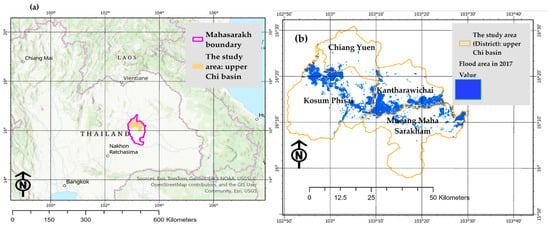
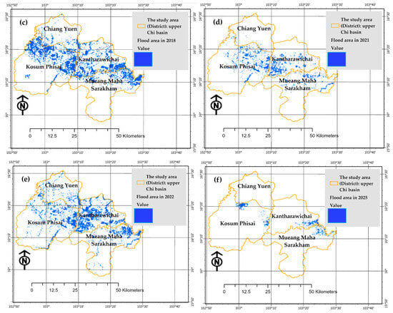
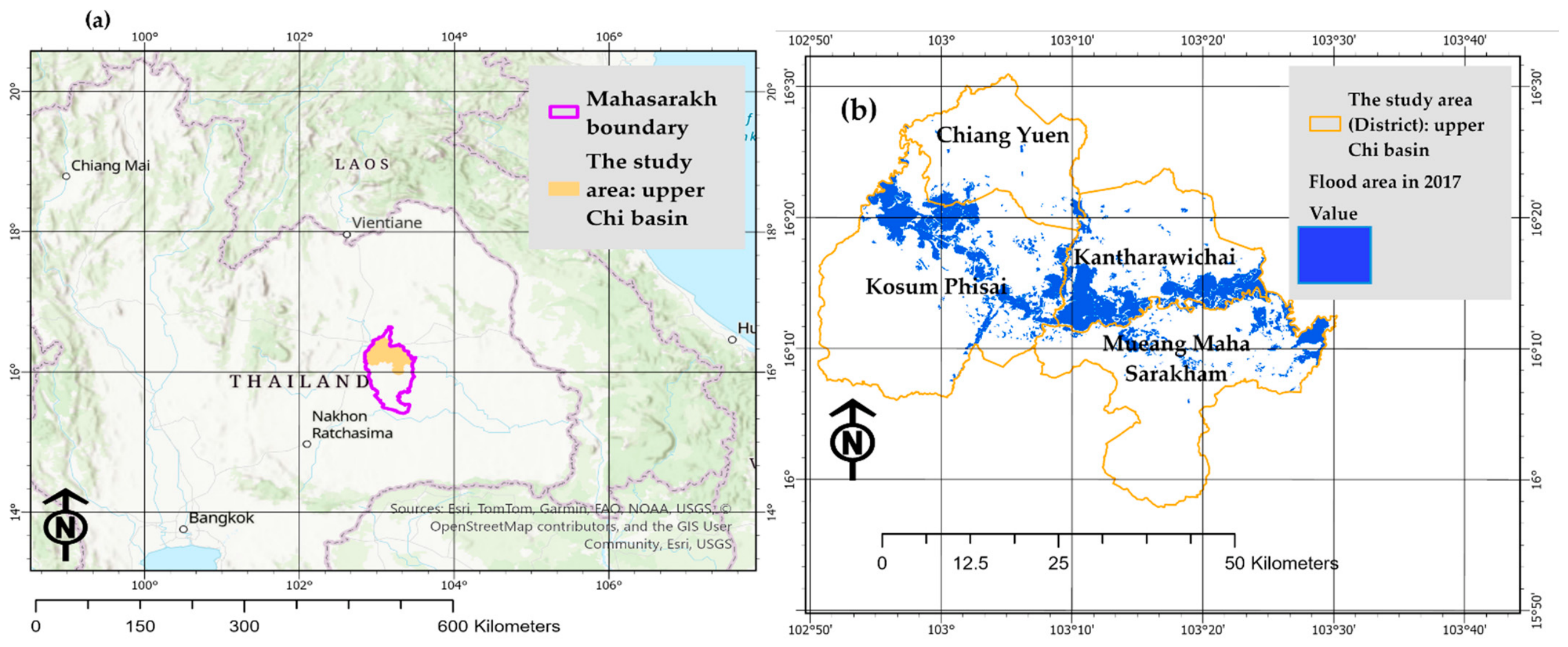
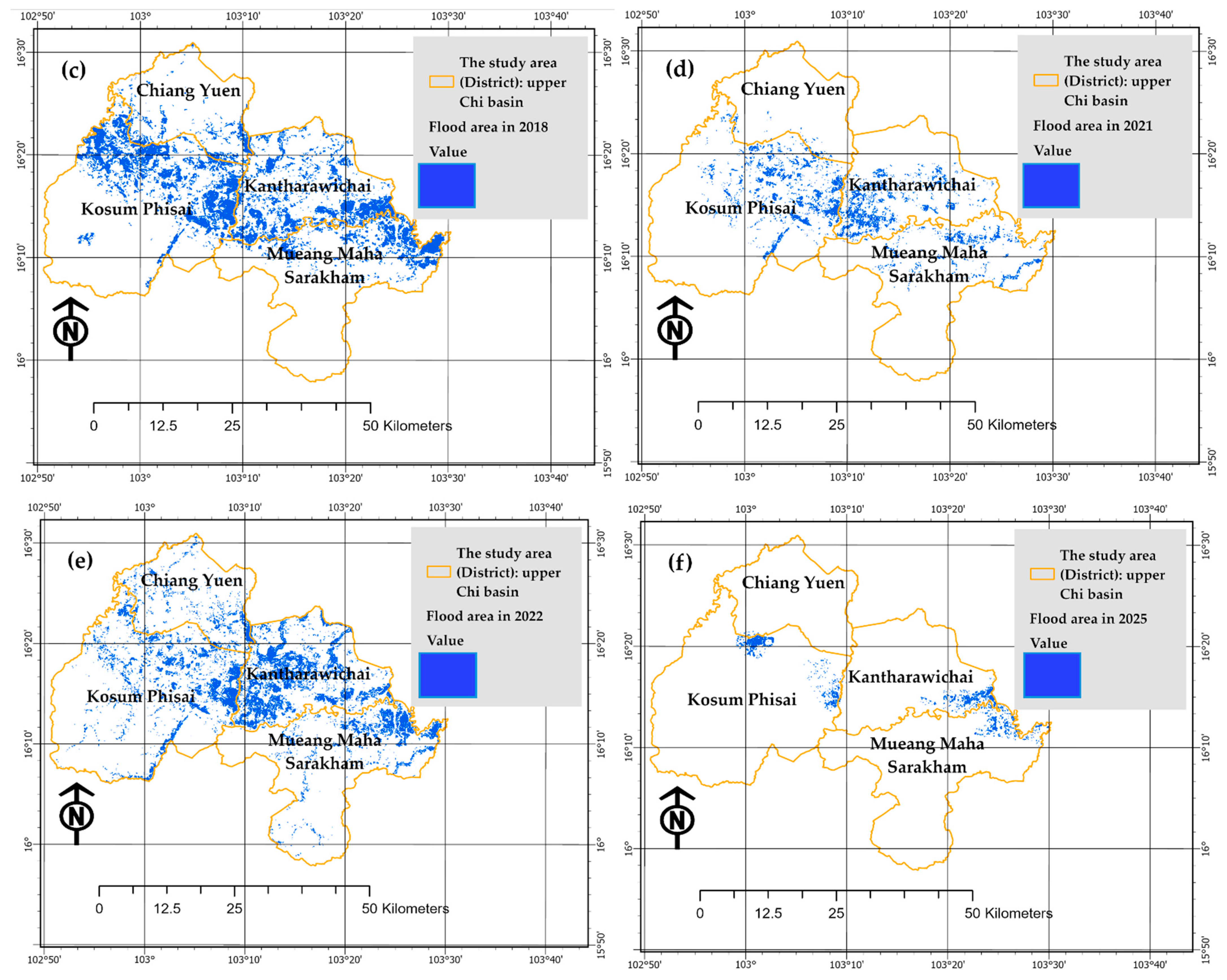
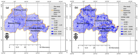
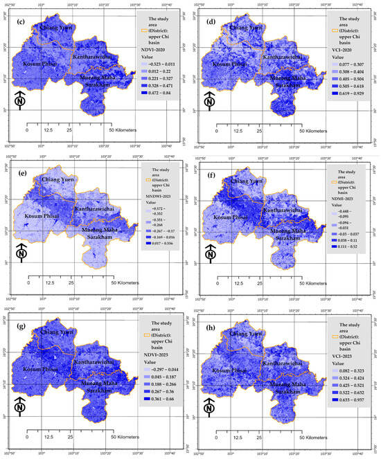
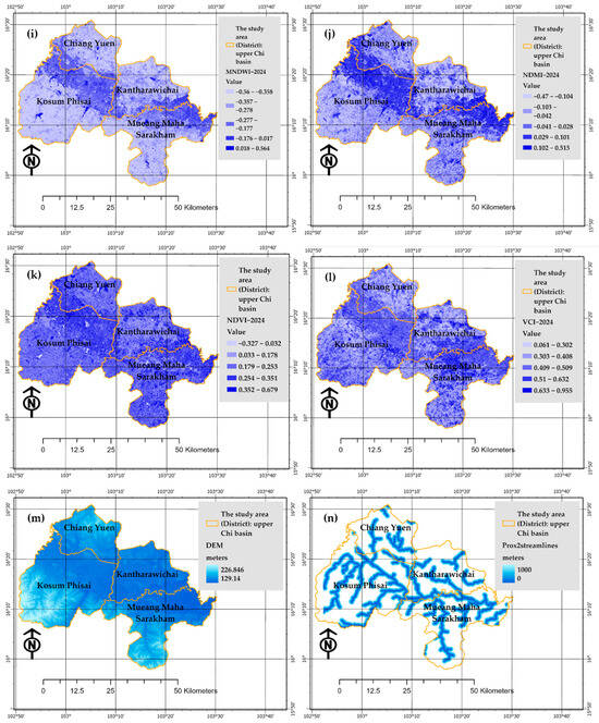
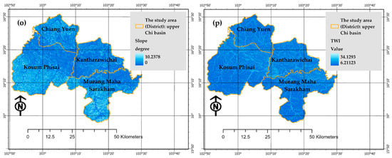
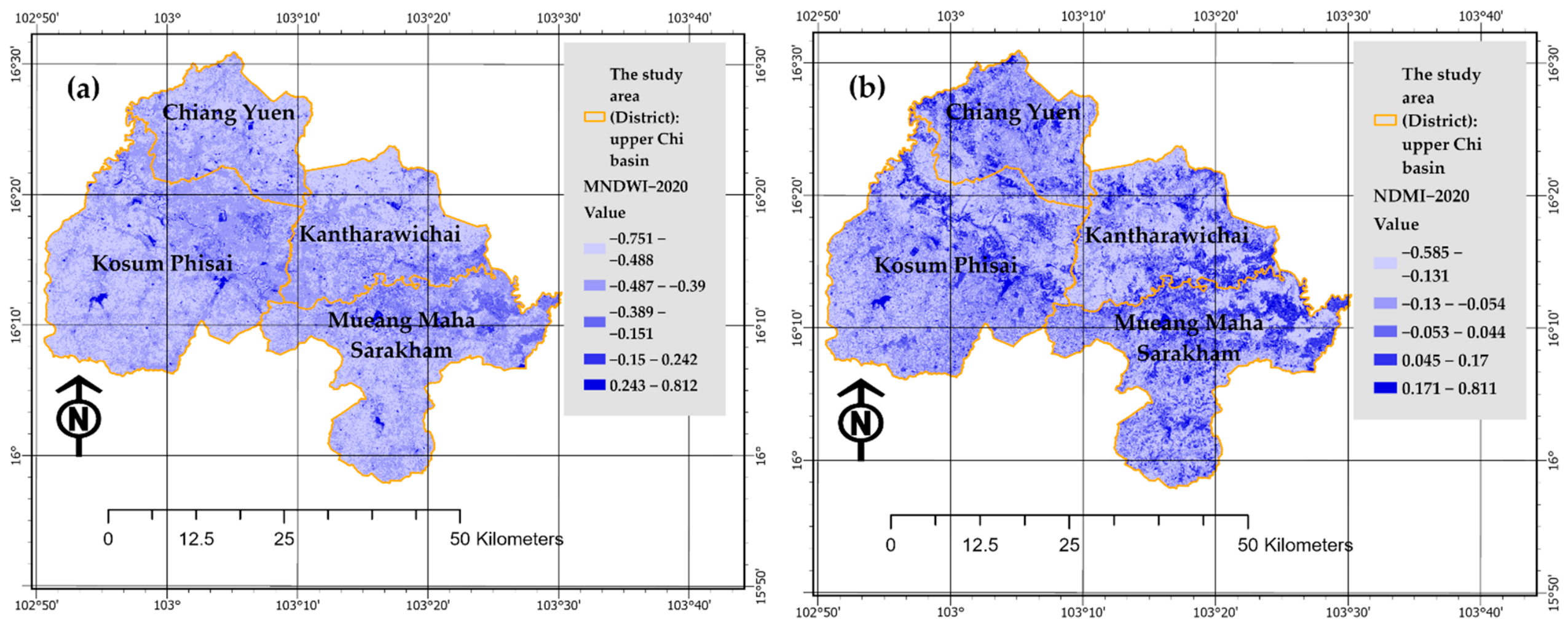
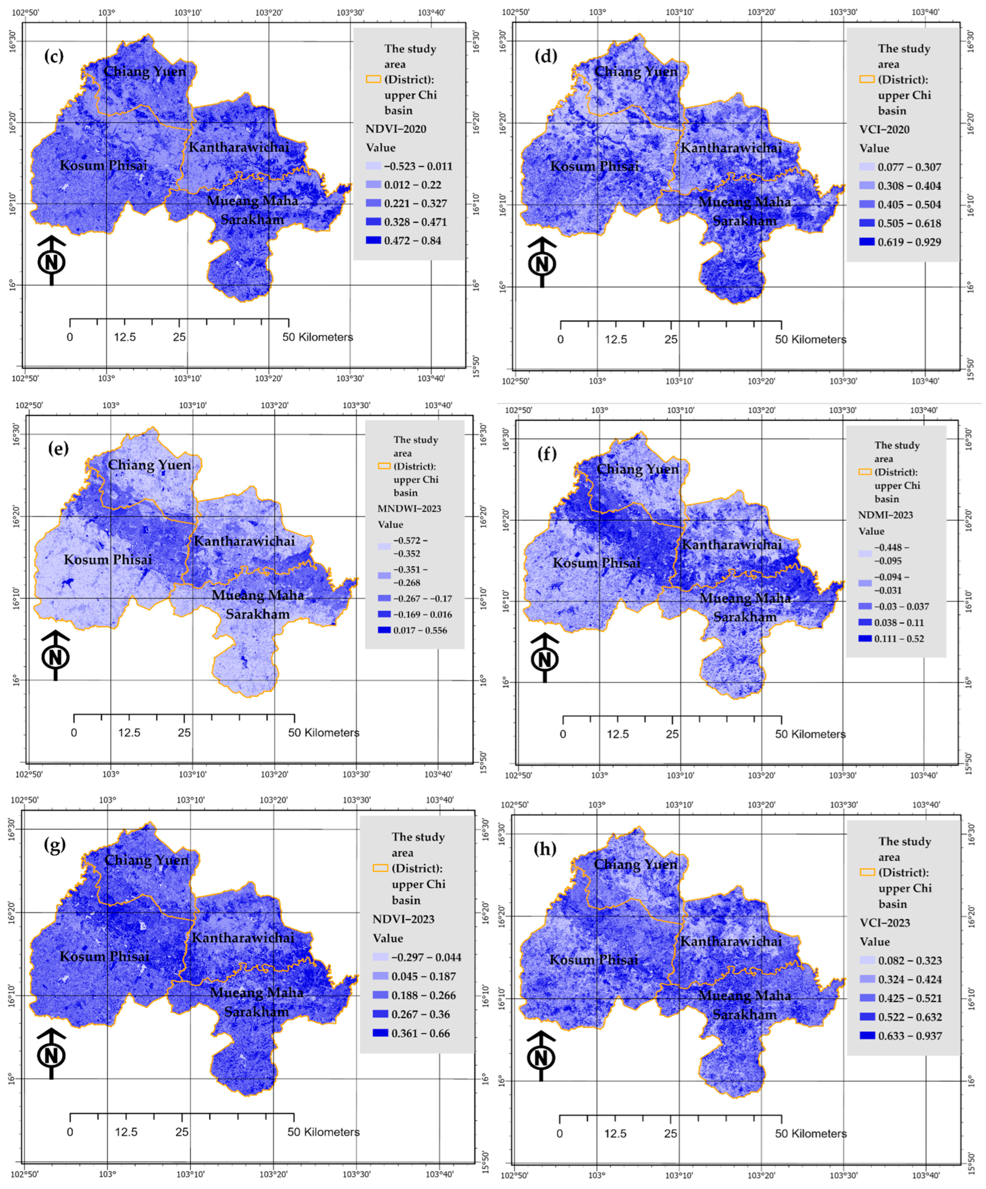
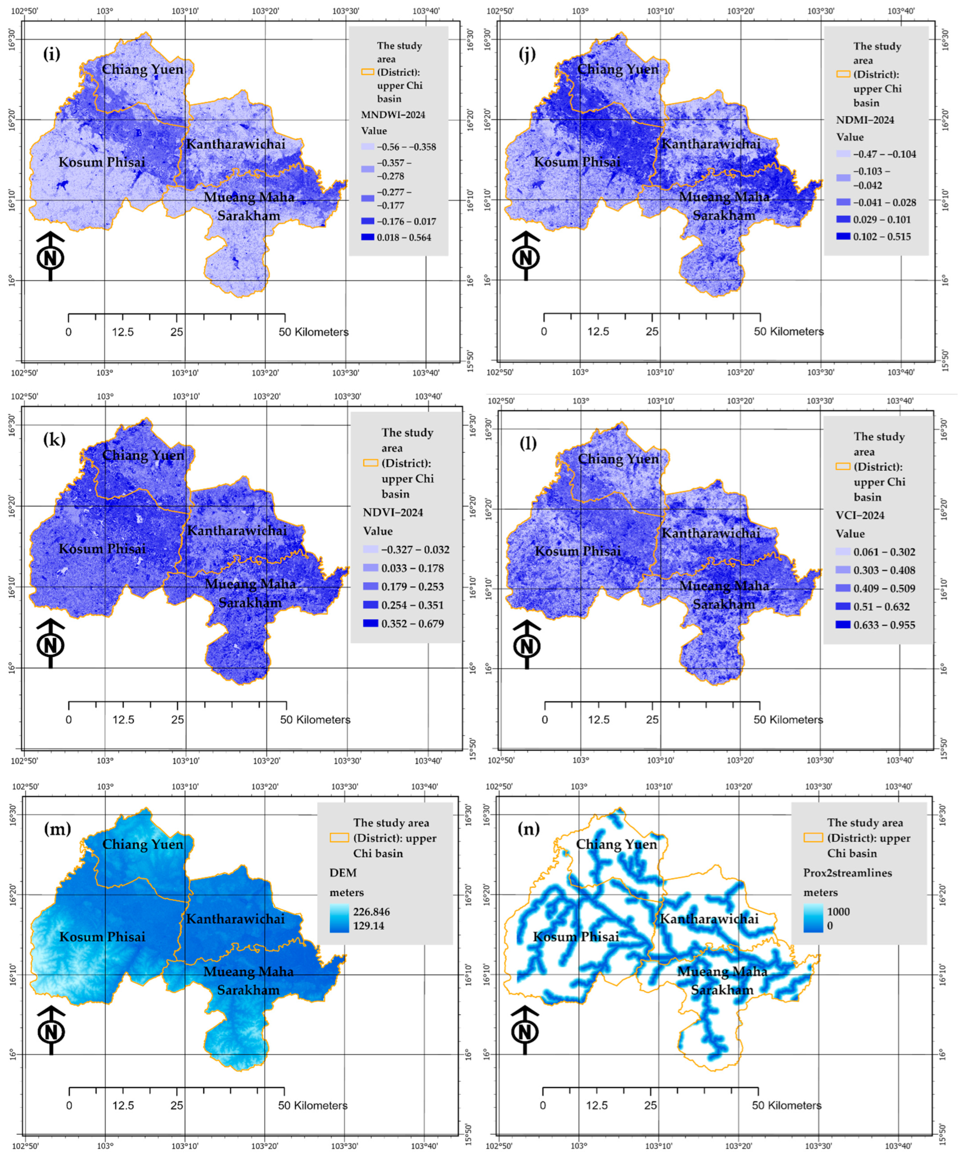
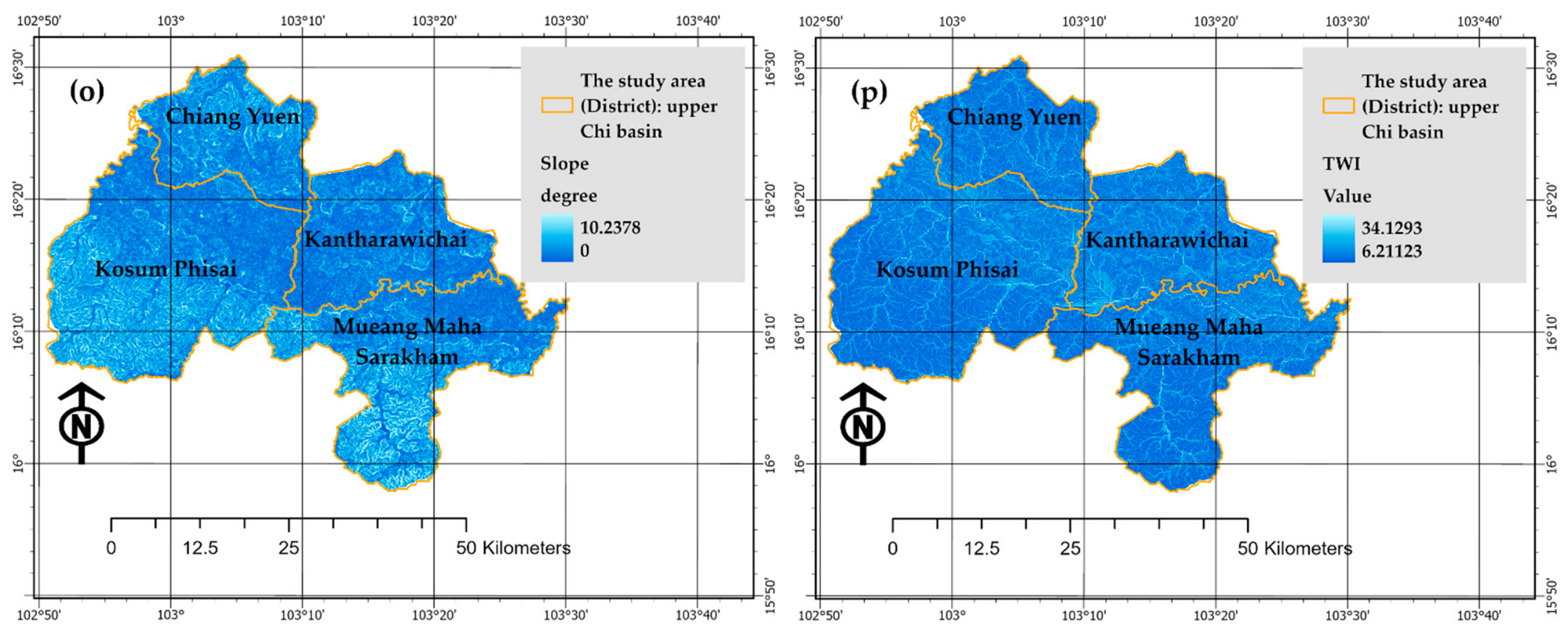
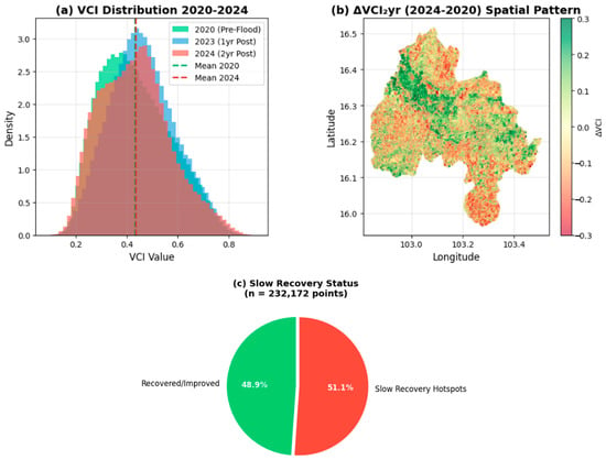
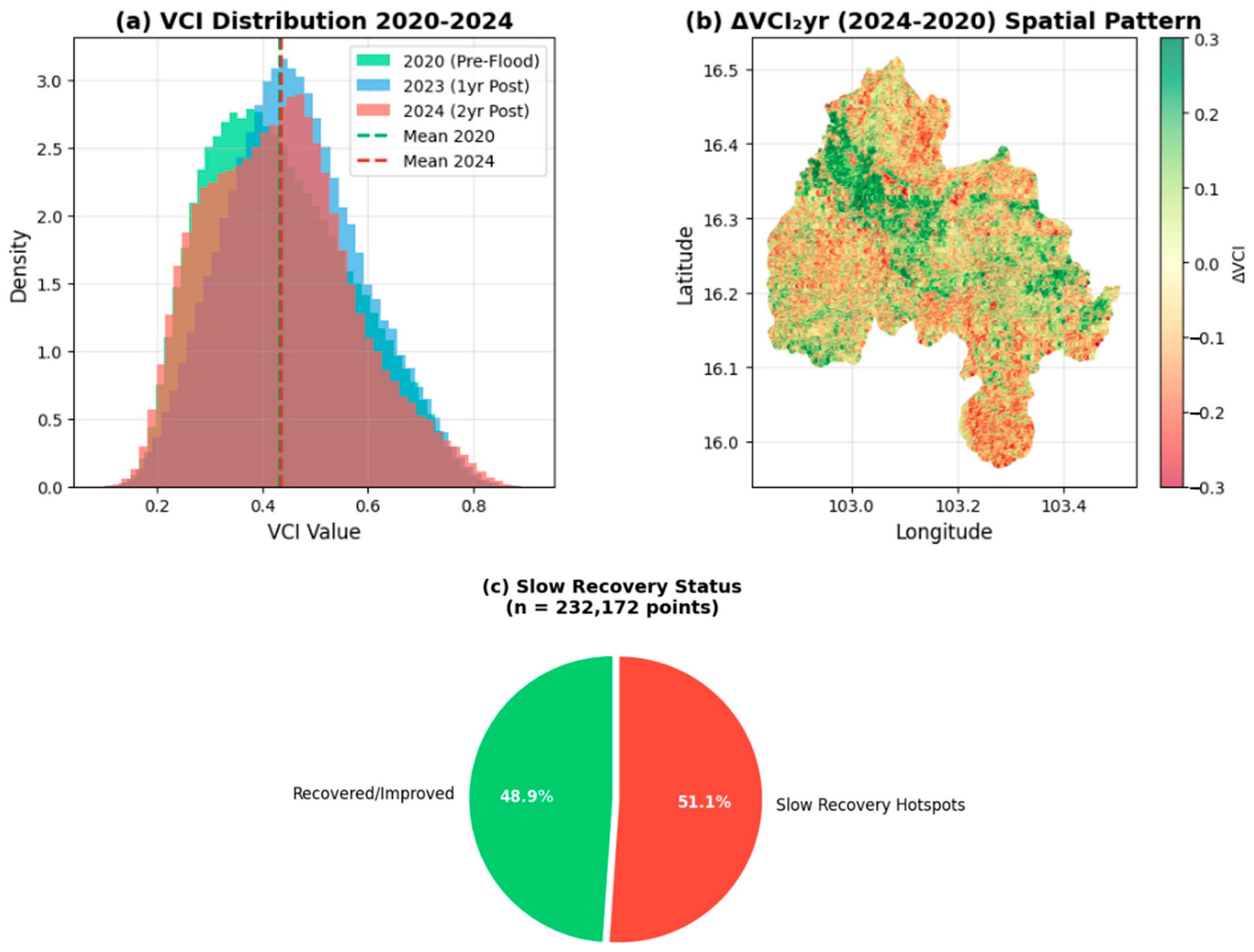
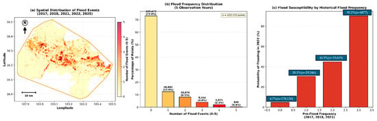
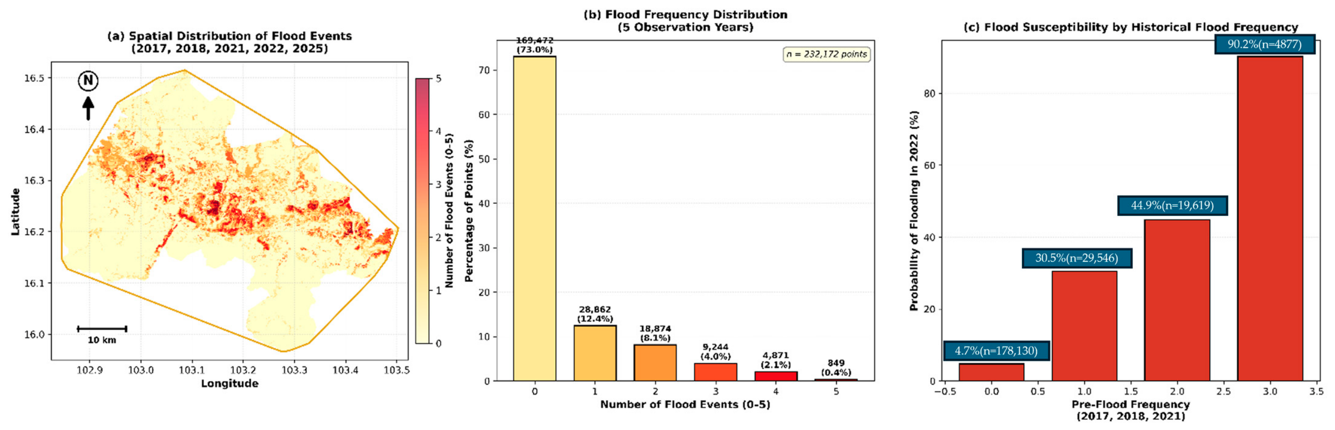
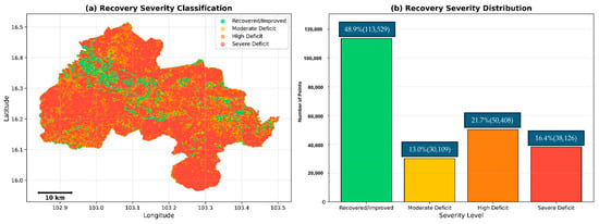
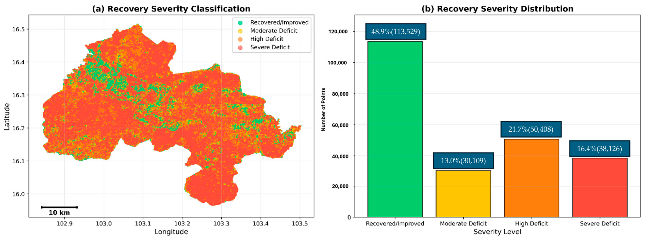
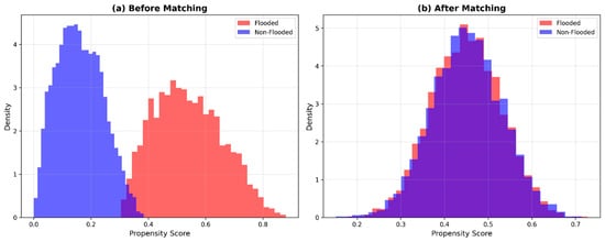
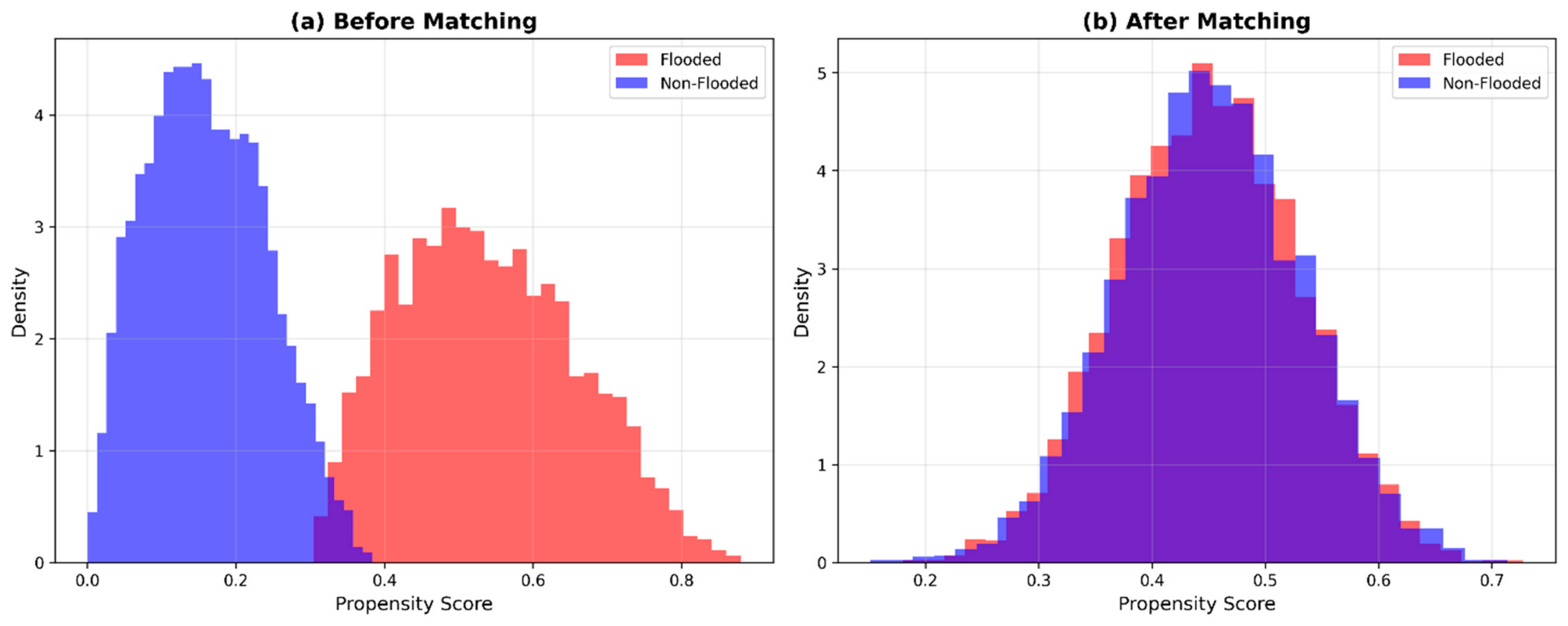
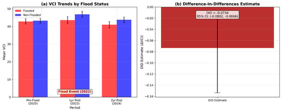
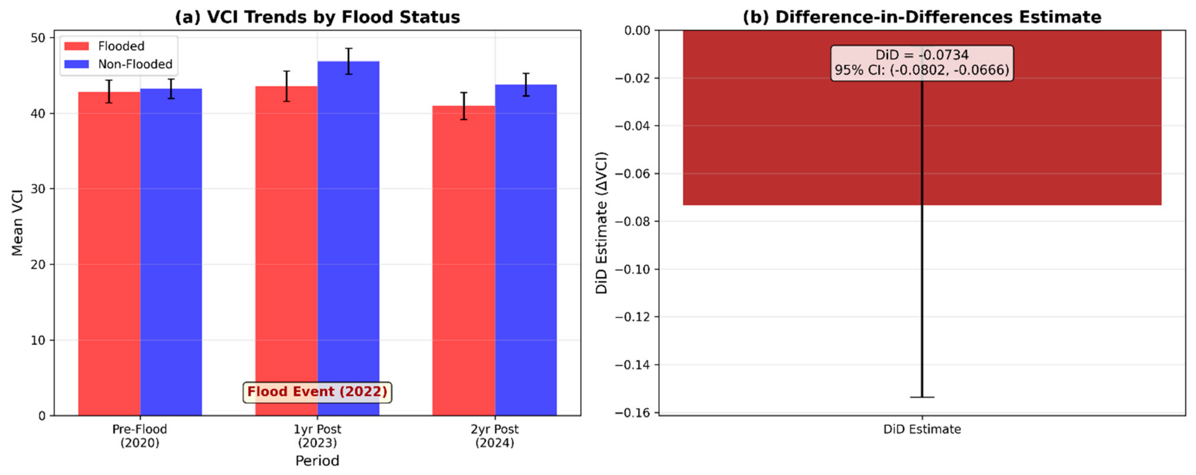
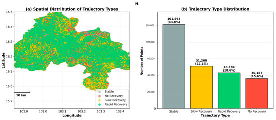
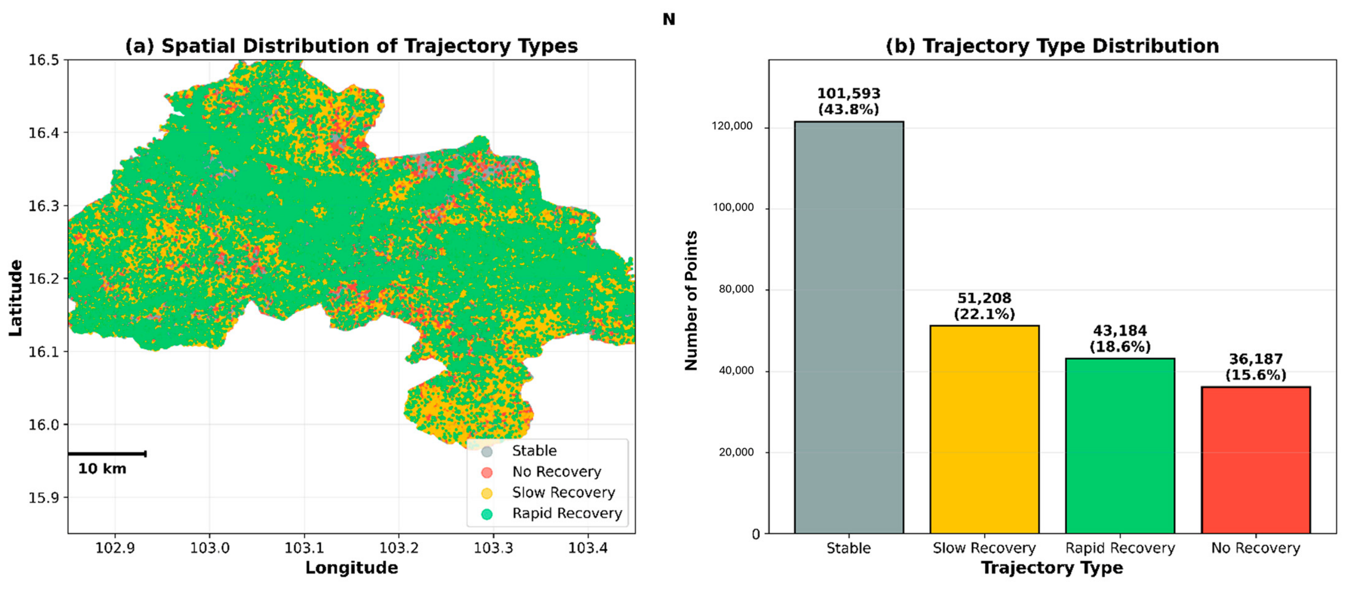
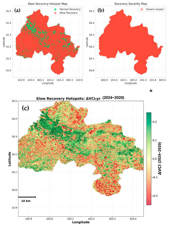
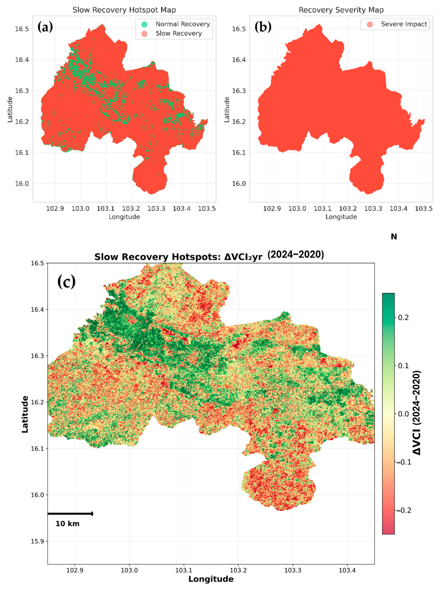
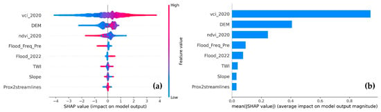
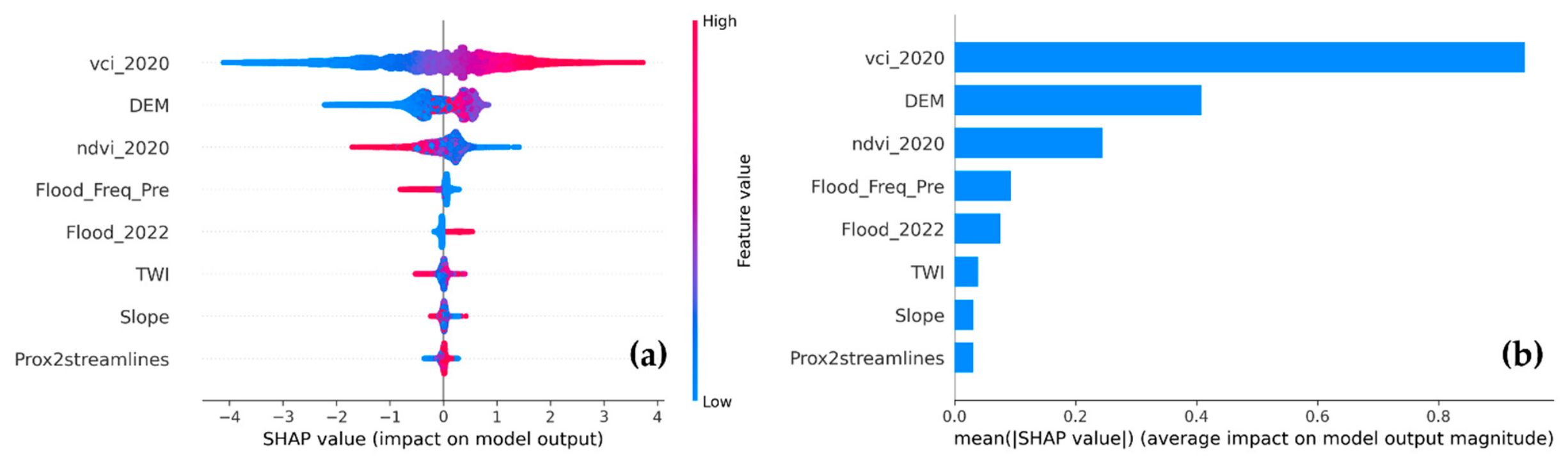
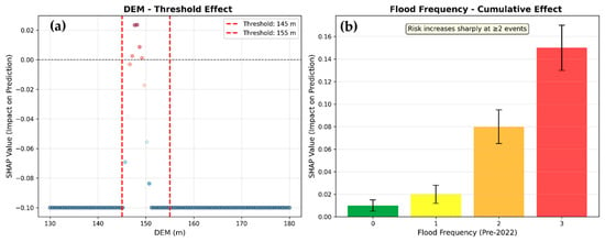
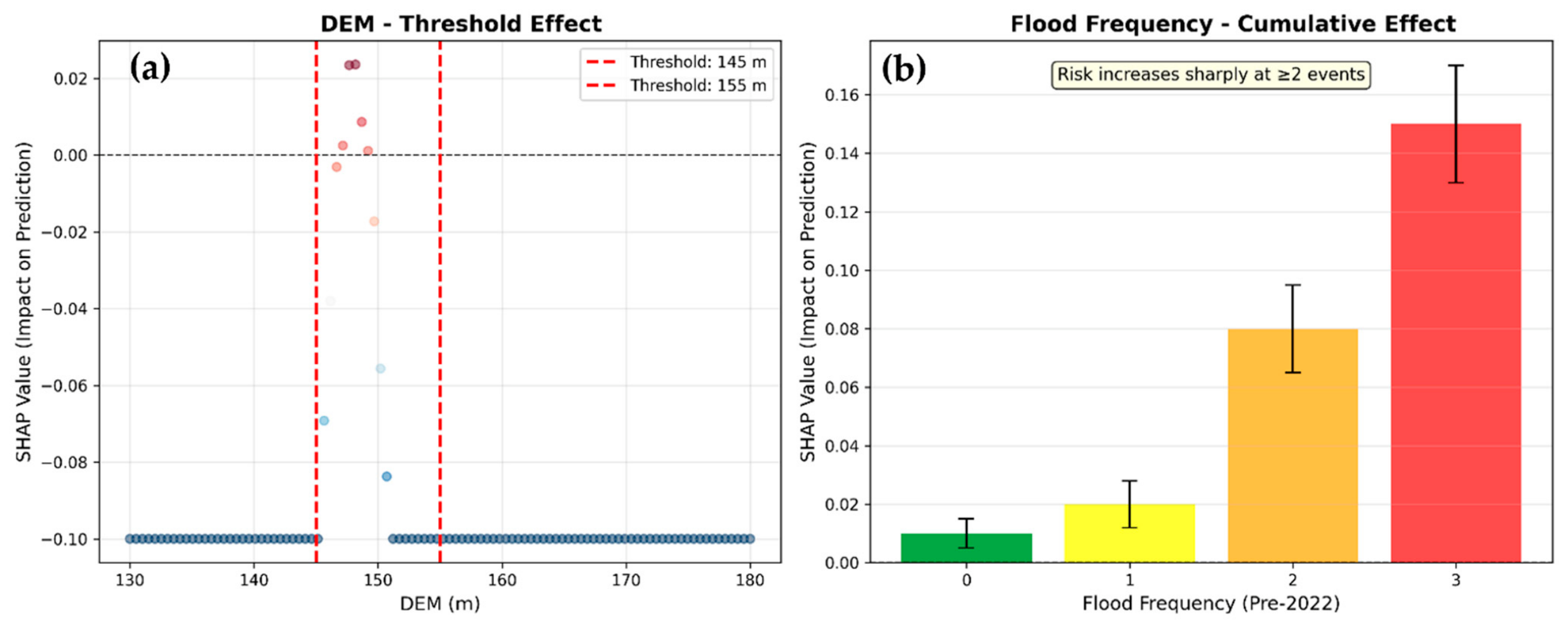
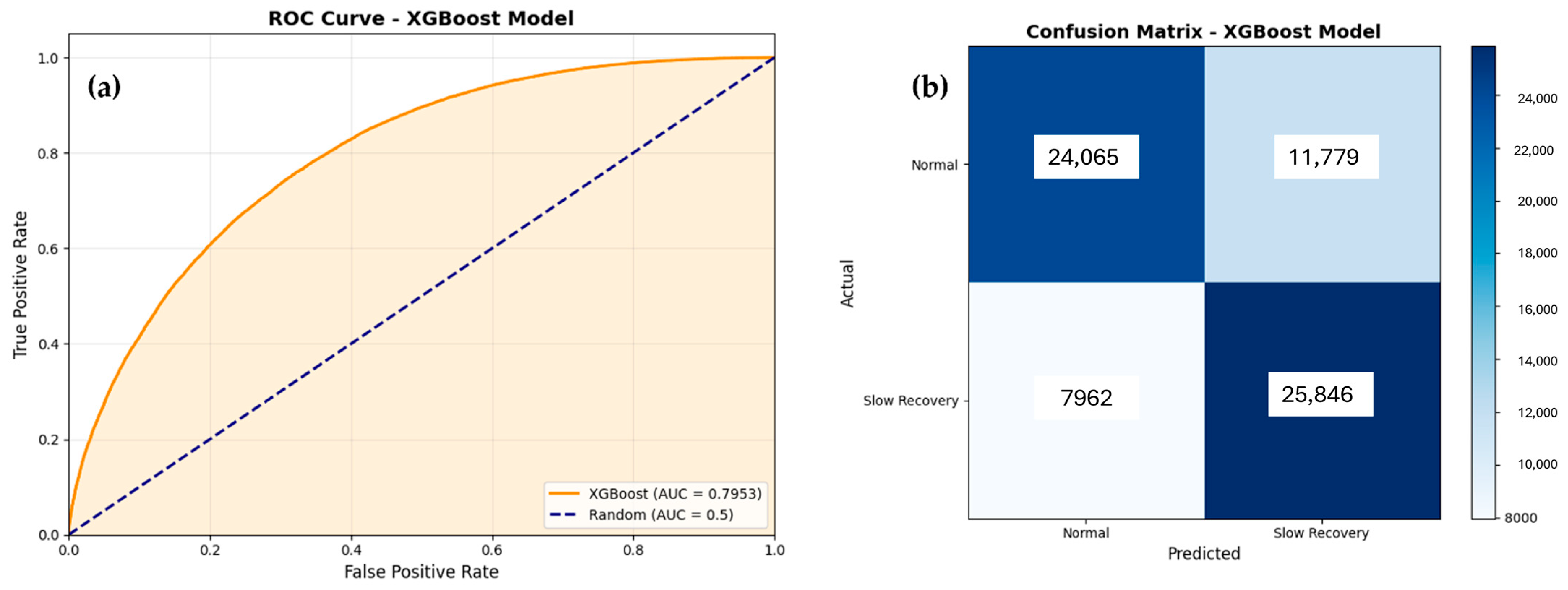
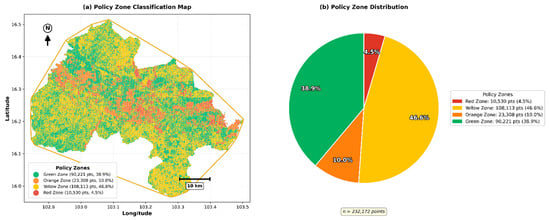
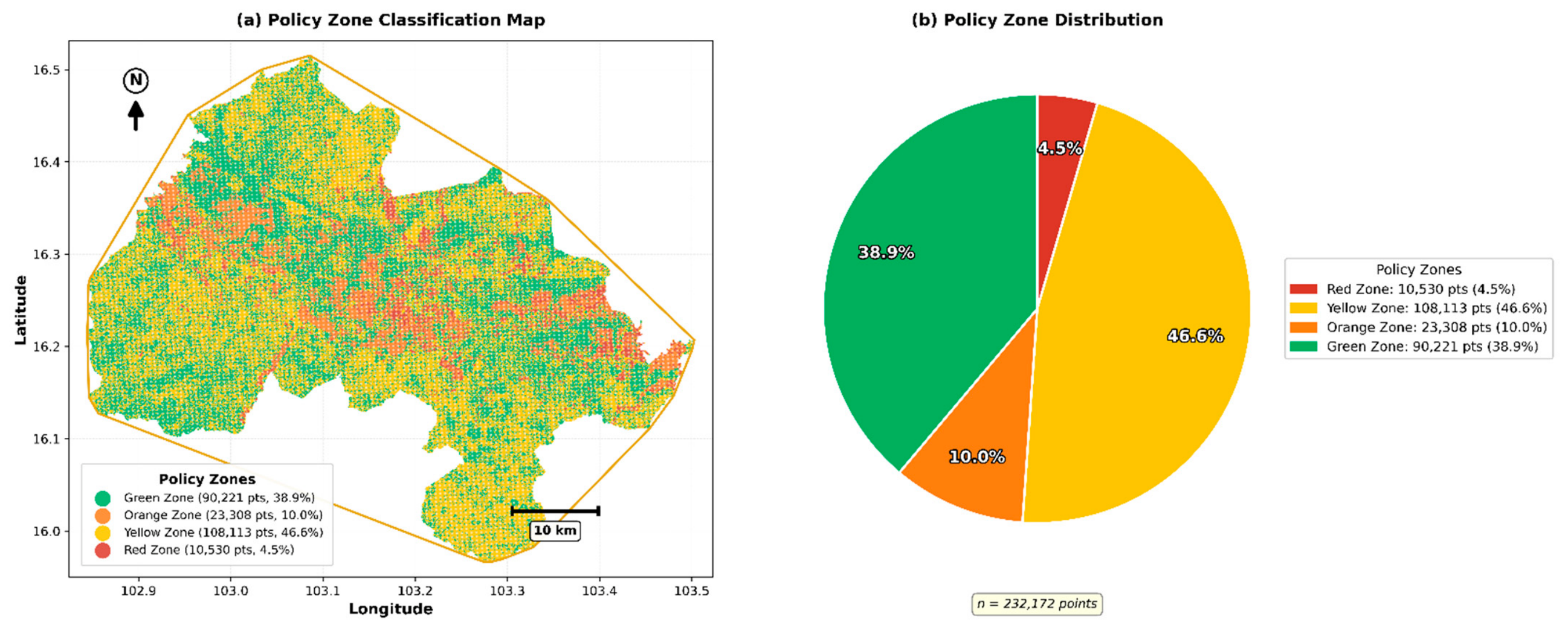

Disclaimer/Publisher’s Note: The statements, opinions and data contained in all publications are solely those of the individual author(s) and contributor(s) and not of MDPI and/or the editor(s). MDPI and/or the editor(s) disclaim responsibility for any injury to people or property resulting from any ideas, methods, instructions or products referred to in the content. |
© 2026 by the authors. Licensee MDPI, Basel, Switzerland. This article is an open access article distributed under the terms and conditions of the Creative Commons Attribution (CC BY) license.