


Abstract
Energy-burdened rural communities require hybrid renewable energy storage solutions that are not only economically viable but also resilient to extended generation shortfalls. This study develops a spatially informed techno-economic and resilience assessment framework for hydrogen–biogas renewable microgrids and applies it to Robeson County, North Carolina. A Hydrogen Priority Index (HPI) is used to identify locations where high household energy burden coincides with favorable renewable energy suitability. Four community-scale microgrid configurations are then evaluated in HOMER Pro under standard economic criteria and an embedded seven-day winter solar shortfall stress scenario. Results show that biogas integration reduces net present cost by 28.4% by restructuring the optimal system architecture and reducing PV and battery oversizing. PV–battery configurations cannot achieve near-complete resilience under the imposed stress scenario regardless of component scaling, while hydrogen-inclusive configurations reduce stress-period unmet load by 97.2%. The full hydrogen–biogas hybrid delivers this resilience-constrained performance at 26% lower net present cost than the hydrogen-only configuration. These findings demonstrate that combining spatial prioritization with resilience-constrained techno-economic assessment supports more equitable and deployment-ready planning of renewable microgrids for underserved rural communities.
1. Introduction
Hydrogen-integrated microgrids represent a technically viable pathway to resilient electrification in underserved communities, yet existing deployment frameworks remain misaligned with the equity-based siting and resilience requirements these communities specifically impose [1,2]. Low-income and rural communities in the southeastern United States face energy burdens exceeding 10% of gross household income, more than three times the national median, while simultaneously lacking the financial capacity to invest in backup systems or participate in clean energy markets [3,4]. North Carolina exemplifies this challenge: with 80 of its 100 counties classified as rural and nearly 1.5 million residents classified as energy-overburdened, the state has among the most acute concentrations of residential energy vulnerability in the country, driven by energy-inefficient housing stock and persistent structural disinvestment [5,6]. Energy burden, defined as the percentage of gross household income allocated to residential energy expenditures, is the established metric for identifying communities where energy costs impose disproportionate financial stress [7]. The U.S. Department of Energy Low-Income Energy Affordability Data (DOE LEAD) dataset provides census-tract-level energy burden estimates that enable spatially explicit identification of high-vulnerability communities [8], forming the equity data foundation of this study’s site selection framework.
Off-grid solar photovoltaic (PV) microgrids have emerged as technically and economically viable pathways to electrification in underserved communities, bypassing costly grid extension while delivering clean generation at community scale [9]. Within this landscape, hydrogen storage has attracted growing attention as a long-duration, resilient energy storage medium capable of bridging multi-day generation deficits that battery systems cannot economically address [9,10]. On the other hand, biogas, produced through anaerobic digestion of organic feedstocks including livestock manure, provides a weather-independent dispatchable complement to intermittent PV generation, making it a natural partner for rural hybrid energy systems where agricultural feedstocks are locally available [11]. Together, these technologies directly address the structural deficiencies that produce chronic energy burdens: hydrogen provides multi-day resilience storage, biogas provides dispatchable renewable firm power, and PV provides cost-effective primary generation.
Despite this technical promise, most design frameworks used to evaluate hydrogen-integrated microgrids have been developed primarily for cost minimization under normal operating conditions, without incorporating the social equity criteria or resilience stress testing that deployment in energy-burdened communities specifically requires [12]. Existing site selection approaches optimize technical and economic suitability without accounting for community vulnerability, systematically bypassing the populations most in need of resilient energy access. At the same time, resilience evaluation in the hydrogen microgrid literature has relied on post hoc scenario analysis rather than on optimization-embedded stress protocols, resulting in designs that are cost-optimal under normal conditions but not inherently stress-hardened. North Carolina’s rural counties offer a compelling and underserved context in which to address this triple gap directly: the state ranks among the highest in residential energy burdens in the southeastern United States, within predominantly agricultural landscapes that offer both strong solar resources and substantial livestock-based biogas potential. This study therefore develops and demonstrates a spatially informed interdisciplinary techno-economic and resilience optimization framework that integrates equity-based site prioritization, community-scale biogas resource quantification, and embedded resilience stress testing within a single hydrogen–biogas microgrid comparative assessment methodology, providing a deployment-ready framework explicitly built for energy-burdened rural communities rather than adapted from frameworks designed for cost-optimal contexts.
1.1. Literature Review
1.1.1. Hydrogen-Integrated Hybrid Renewable Systems
The techno-economic feasibility of hydrogen-integrated off-grid microgrids has been extensively evaluated using simulation-based optimization platforms, most prominently HOMER Pro (Hybrid Optimization Model for Multiple Energy Resources), a widely used medium for techno-economic optimization of hybrid energy systems [13,14]. A hydrogen-integrated microgrid typically couples a PV array with a proton exchange membrane (PEM) electrolyzer, compressed hydrogen storage tank, and PEM fuel cell: during surplus generation periods, excess PV output drives electrolysis; stored hydrogen is later reconverted via the fuel cell during generation shortfalls [15,16]. This architecture enables multi-day and seasonal energy storage at scales that lithium-ion battery systems cannot cost-effectively achieve, making it particularly relevant for sites subject to extended low-irradiance periods [10,17]. Recent HOMER Pro-based feasibility studies confirm the viability of off-grid hydrogen-integrated hybrid systems across diverse resource-constrained contexts [18]. Comprehensive reviews of hybrid hydrogen-battery storage optimization approaches further identify resilience stress testing and equity-based siting as consistently unaddressed gaps in existing frameworks [19], where optimization under normal operating conditions remains the dominant paradigm.
Ghenai et al. demonstrated for a residential desert community that hydrogen storage improves system reliability at a cost premium relative to PV–battery configurations, quantifying the trade-off between reliability and levelized cost of energy (LCOE) [20]. Lokar and Virtic established that hydrogen is essential for complete seasonal energy self-sufficiency in residential buildings at mid-latitude locations where winter solar constraints cannot be bridged by battery storage alone [17]. Babatunde et al. showed that applying multi-criteria sustainability objectives shifts the optimal off-grid configuration from PV–battery to PV–fuel cell hybrid, underscoring the inadequacy of single-criterion cost optimization frameworks for communities that require reliability alongside affordability [12]. Abdin and Merida conducted a techno-economic comparison across multiple hybrid off-grid configurations and demonstrated that hydrogen becomes cost-competitive under specific resource and load conditions, with LCOE sensitivity strongly dependent on discount rate and component cost assumptions [21]. Möller et al. further demonstrated that seasonal hydrogen storage enables complete off-grid self-sufficiency for prosumer systems in Germany and Finland, confirming the technology’s scalability across diverse climatic contexts [10]. Collectively, these studies establish that cost-optimal and resilience-optimal system designs diverge significantly as reliability constraints tighten. However, the specific reliability constraint level at which hydrogen storage transitions from an economic trade-off to an operationally necessary component, and whether PV–battery configurations can satisfy resilience-constrained operation under extended solar shortfall, has not been empirically examined under optimization-embedded stress conditions in any existing study.
1.1.2. Biogas-Integrated Hybrid Renewable Systems
Biogas-integrated hybrid microgrids have been evaluated across a range of scales, feedstock types, and geographic contexts. Nassereddine et al. demonstrated that a PV–biogas hybrid system maintains stable power supply during solar generation shortfalls without requiring additional storage, confirming the dispatchability advantage of biogas over weather-dependent renewables [22]. Mukhtar et al. optimized a PV–biogas–hydropower–battery system for a rural village in northwest Pakistan using HOMER Pro, achieving cost-effective electrification through multi-source dispatch; the study highlighted that biogas contributes disproportionately to system reliability relative to its generation share [23]. Ennemiri et al. optimized a PV–biogas–battery system for a commercial platform in Morocco, finding that biogas integration reduced CO2 emissions by 40% relative to a biogas-only reference and that capital subsidies significantly affect economic viability [24]. Tiam Kapen et al. demonstrated the technical feasibility of a combined PV–battery–fuel cell–electrolyzer–biogas system in Cameroon using HOMER Pro, one of the few studies to integrate both biogas and hydrogen within a single hybrid configuration [25]. Despite these contributions, the architectural mechanism through which biogas dispatch restructures the entire optimal system design, reducing PV capacity, halving battery bank size, and shifting dispatch strategy, rather than simply adding generation capacity, has not been explicitly characterized. Furthermore, no existing study has integrated county-level livestock feedstock quantification with proportional community-scale downscaling for direct simulation input, maintaining methodological traceability from agricultural census data to system design parameters.
1.1.3. Geospatial Siting Frameworks for Hydrogen Systems
Geographic Information System (GIS) methods combined with multi-criteria decision analysis (MCDA) have been applied to renewable hydrogen facility siting in a growing body of literature. Messaoudi et al. developed a GIS-MCDA framework for solar hydrogen siting in Algeria, finding that only 0.49% of assessed land qualified as highly suitable under combined technical and environmental constraints, demonstrating the critical importance of spatially explicit screening over uniform deployment assumptions [26]. Rezaei et al. applied a hybrid wind–solar MCDA using HOMER and Fuzzy-TOPSIS to identify optimal hydrogen generation sites across 31 capital cities, demonstrating the tractability of multi-criteria spatial optimization at regional scale [27]. Fotsing Flora et al. applied a GIS-based framework incorporating Monte Carlo simulation and fuzzy AHP to rank optimal sites for solar–wind hybrid hydrogen production in Cameroon, showing that probabilistic uncertainty handling substantially improves site ranking robustness over deterministic MCDA approaches [28]. While these studies demonstrate the value of spatially explicit siting, they address resource and technical feasibility exclusively, without incorporating community socioeconomic vulnerability as a co-equal criterion. The spatial coincidence of high energy burden and strong renewable resource potentially identifying communities where deployment is simultaneously most needed and most viable has not been operationalized as a composite siting index in any prior hydrogen energy study. Frameworks that prioritize communities on social grounds alone risk selecting sites with weak resource bases; those that optimize on technical and economic grounds tend to bypass the communities most in need.
1.1.4. Microgrid Resilience Design and Stress Testing
Microgrid resilience, defined as the ability to maintain adequate load service during adverse operating conditions, has emerged as a distinct and increasingly prioritized design objective beyond conventional cost optimization [29,30]. Hirsch et al. reviewed resilience technologies and metrics for microgrids and concluded that conventional techno-economic studies systematically undervalue storage technologies by evaluating their performance under normal operating conditions rather than stress events, where storage transitions from a cost-optimization lever to a survival mechanism [31]. Khodaei et al. proposed a resilience-oriented planning framework for distribution microgrids that explicitly models extreme events, finding that multi-day outage survivability requires fundamentally different system architectures than those produced by LCOE minimization alone [32]. Panteli and Mancarella further articulated the conceptual distinction between reliability, which addresses routine contingencies, and resilience, which addresses low-probability high-impact events, arguing that resilience-oriented design requires dedicated planning methodologies rather than extensions of standard reliability optimization [29]. In the hydrogen microgrid literature, resilience evaluation has typically been conducted through post hoc analytical scenarios applied to pre-optimized economic designs rather than embedded directly within the optimization process. This approach structurally fails to produce stress-hardened designs, because the optimizer has no incentive to size storage for survivability beyond the modeled normal-year conditions. An embedded, physics-grounded stress protocol that forces the optimizer itself to target survivability under defined worst-case conditions does not yet exist in the hydrogen microgrid literature.
1.2. Research Gaps and Contributions
The review above identifies a coherent and unaddressed macro-gap: no existing interdisciplinary optimization framework integrates equity-based spatial prioritization, resilience-constrained comparative evaluation, and hydrogen–biogas technology interaction characterization within a single community microgrid design methodology. This study addresses that gap by developing a spatially informed techno-economic and resilience optimization framework for hydrogen–biogas microgrid hybrid renewable energy storage in energy-burdened rural communities, applied to North Carolina as a representative case, through four integrated components: (i) spatial equity-based site prioritization using the Hydrogen Priority Index; (ii) local biogas resource quantification from county-level livestock census data; (iii) comparative hydrogen–biogas microgrid configuration assessment across four system architectures; and (iv) embedded seven-day solar shortfall stress testing within the HOMER Pro optimization year. The specific study objectives are: (i) to construct a Hydrogen Priority Index (HPI) combining socioeconomic vulnerability and multi-criteria technical suitability to identify priority deployment sites; (ii) to quantify community-scale biogas potential from livestock feedstocks and incorporate it into HOMER Pro optimization across different microgrid architectures under both economic and resilience constraints; and (iii) to evaluate the cost and resilience implications of hydrogen storage through an embedded solar shortfall protocol that forces resilience-aware optimization under identical boundary conditions across all configurations.
This study makes four principal novelty contributions: (a) the first composite siting index that operationalizes social equity and technical feasibility as co-equal criteria for hydrogen–biogas microgrid deployment, enabling site selection that cost-only approaches structurally cannot perform; (b) an embedded physics-grounded solar shortfall protocol that empirically identifies a configuration-level feasibility threshold under the modeled Robeson County conditions, beyond which hydrogen storage becomes the operationally necessary component for resilience-constrained performance; (c) a controlled four-scenario decomposition revealing the complementary rather than substitutable temporal roles of hydrogen storage and biogas dispatch; and (d) equity-oriented, planning-relevant insights for rural electrification in energy-burdened agricultural communities, delivered through an analytical framework built on publicly available national datasets (DOE LEAD, NSRDB, NLCD, PAD-US) and therefore reproducible for other U.S. counties, while the numerical results reported here remain specific to Robeson County.
2. Material and Methods
2.1. Methodological Overview
Building on the literature reviewed in Section 1, the study asks how electrochemical hydrogen equipment and biogas-linked firm generation shift least-cost microgrid layouts and electricity service during stretched low-irradiance conditions, relative to a PV–battery baseline, for a fixed rural community load. County selection follows multi-criteria geospatial screening integrating energy burden and technical suitability [33]; biogas supply is quantified through livestock inventories and a standard manure-screening tool [34]; dispatch and hybrid renewable energy storage economics are optimized in HOMER Pro [13]. The solar resource uses a full hourly annual trace with an embedded seven-day reduced-GHI window, an explicit resilience stress protocol rather than an incidental modeling artifact.
The study proceeds in three phases. Phase 1 justifies Robeson County as the priority deployment site, quantifies livestock-linked biogas potential and HOMER Pro biomass inputs, and fixes the NSRDB solar node used across all scenarios. Phase 2 assembles the community load and solar series including the embedded low-GHI window and optimizes four microgrid configurations under shared economic and reliability constraints. Phase 3 compares configurations on cost outcomes and stress-period performance to identify the reference architecture under the defined criteria. All inputs are drawn from public geospatial, agricultural, meteorological, and catalog-based techno-economic sources. Visualization of HOMER Pro simulation output (Figures 5, 9, 10 and 12–14) was performed with the assistance of a generative AI tool (Claude, Anthropic-sonnet 5).
2.2. Study Area and Community Load Profile
Robeson County, North Carolina, was selected as the representative case study based on the composite Hydrogen Priority Index (HPI) derived from the geospatial screening framework described in Section 2.2.1. The county, located in the southeastern coastal plain of North Carolina (approximately 34.75° N, 79.25° W), is home to approximately 42,509 households and ranks among the most energy-burdened jurisdictions in the state. A representative community of 200 households was defined to reflect a realistic off-grid microgrid deployment scale consistent with rural electrification targets in underserved regions.
2.2.1. Geospatial Site Selection Framework
A two-stage GIS-based screening framework was developed to systematically identify priority locations for hydrogen microgrid deployment across North Carolina. The framework integrates spatially explicit socioeconomic vulnerability assessment with engineering-based technical suitability modeling, performed in ArcGIS Pro v3.5.0 (Esri, Redlands, CA, USA). The combined output—“Hydrogen Priority Index”—identifies locations where high community energy vulnerability coincides with strong renewable energy potential and favorable infrastructure conditions.
Stage 1: Energy burden analysis
Energy burden data at the census-tract level were obtained from the U.S. Department of Energy Low-Income Energy Affordability Data (DOE LEAD) dataset [8] and spatially joined to TIGER/Line census tract boundaries using the GEOID identifier [35]. Energy burden is defined as the percentage of gross household income allocated to residential energy expenditures. It was used as the primary indicator of energy vulnerability. To enable integration with engineering suitability scores, raw burden values were normalized using min–max scaling:
where EBI_i is the normalized Energy Burden Index for tract i, and EB_min and EB_max represent the statewide minimum and maximum values, respectively.
EBI_i = (EB_i − EB_min)/(EB_max − EB_min)
Global Moran’s I was computed to assess spatial dependence in the EBI distribution (Appendix A); results confirmed statistically significant clustering of high-burden tracts, supporting the use of spatially targeted rather than dispersed deployment strategies. Localized clusters of elevated energy burden were subsequently identified using Getis–Ord Gi* statistics; census tracts with a Gi* z-score exceeding 1.96 (p < 0.05) were classified as statistically significant hotspots, constituting the social prioritization layer for subsequent integration with the technical suitability assessment represented in Figure 1.
Figure 1.
Energy burden hotspot map—Gi analysis, North Carolina.
Stage 2: Technical Suitability Modeling
Technical feasibility for hydrogen microgrid siting was evaluated through a multi-criteria decision analysis (MCDA) framework. Seven spatial criteria were selected to represent renewable resource potential, grid interconnection feasibility, constructability, and environmental constraints (Table 1).
Table 1.
MCDA suitability criteria, scoring logic, data sources, and assigned weights.
Protected areas (PAD-US) were treated as hard exclusion zones and masked prior to suitability scoring. Surface water features were incorporated through Euclidean distance rasters, reflecting increased siting risk rather than categorical restriction. Each remaining criterion was reclassified to a standardized ordinal suitability scale (1–3), where higher values indicate greater suitability for photovoltaic-driven hydrogen systems.
Weights reflect engineering relevance, with solar irradiance prioritized highest (35%) for its direct influence on PV-driven hydrogen production, followed by transmission proximity (25%), land cover (15%), hydrological constraints (12%), road accessibility (10%), and substation proximity (3%).
This weighting scheme was not derived through a study-specific Analytic Hierarchy Process (AHP) exercise; rather, it was informed by convergence with published expert-elicited weighting schemes for comparable solar and hydrogen siting MCDA studies. AHP-based solar suitability assessments consistently assign the dominant weight to solar resource availability, e.g., Munkhbat and Choi assigned 43% to global horizontal irradiance among seven criteria, with transmission-line proximity (12%) and road proximity (9%) as secondary infrastructure criteria [36], and grid/transmission proximity is similarly established as a dominant secondary criterion in other similar studies (e.g., Adebimpe and Usman, where transmission-line distance received 63.3% of combined infrastructure/economic-factor weight [37]). The weighting scheme adopted here reflects this precedent combined with engineering judgment specific to PV-driven hydrogen production.
A weighted linear combination (WLC) was applied to produce the continuous suitability score (SS) raster:
where xk is the standardized suitability score for criterion k and wk is its assigned weight. The weighted linear combination result for North Carolina is represented on the technical suitability map in Figure 2.
Figure 2.
Technical suitability map—weighted linear combination result, North Carolina.
To assess the sensitivity of the county ranking to the expert-assigned weighting scheme, a supplementary equal-weight test was conducted in which six of the seven MCDA criteria were each assigned a weight of 14% and GHI was assigned 16%, producing a total of 100%. This integer-rounded uniform distribution was applied to the same score matrix used in the primary HPI calculation to determine whether the priority ranking is robust to the solar-irradiance-dominant weighting scheme in Table 1.
Hydrogen Priority Index. The Hydrogen Priority Index (HPI) was computed by multiplying the normalized tract-level EBI by the mean technical suitability score extracted to each census tract via Zonal Statistics and joined via the GEOID identifier:
where EBI_i ∈ [0, 1] is the normalized Energy Burden Index and SS_i ∈ {0, 1, 2, 3} is the ordinal technical suitability class assigned to census tract i. The multiplicative formulation therefore produces HPI values ranging from 0 to 3, where higher values indicate communities where both energy burden and renewable resource potential are simultaneously elevated. Because HPI is a simple product of its two components, its proportional (elastic) sensitivity to each is identical: a given percentage change in EBI produces an equal percentage change in HPI, and likewise for SS (formally, the elasticity of HPI with respect to each factor is exactly 1). The multiplicative formulation therefore weights community energy burden and technical suitability equally in relative terms; neither factor structurally dominates the index’s responsiveness to input variation. Marginal (absolute) sensitivities differ only due to each factor’s scale (EBI in [0, 1]; SS in {0, 1, 2, 3}), not due to any asymmetry in the underlying formula. The resulting HPI was aggregated to the county level for ranking and case study selection represented in Figure 3.
HPI_i = EBI_i × SS_i
Figure 3.
Hydrogen Priority Index map—census tract level, North Carolina.
2.2.2. Community Load Profile and Data Collection
The community electrical load profile was derived from the U.S. Department of Energy Low-Income Energy Affordability Data (DOE LEAD) 2022 county-level dataset [8], filtered to prioritized Robeson County households at or below 60% of Area Median Income (AMI), the population segment most represented in the county’s energy burden hotspot zones (Section 2.2.1). Unit-count-weighted electricity expenditure (ELEP × UNITS) and income (HINCP × UNITS) columns were used to compute household-level averages across tenure categories.
Average annual electricity consumption was derived by dividing the weighted expenditure ($1690.89/household/year) by the Robeson County residential electricity rate ($0.1381/kWh) [38], yielding 12,243.95 kWh/household/year. Scaled to 200 households, this produces a community daily demand of 6710 kWh/day and a peak of 829.8 kW, with a cohort energy burden of 10.78%, consistent with the county’s elevated EBI. Derived load parameters are summarized in Table 2, and the resulting daily and seasonal profiles are shown in Figure 4.
Table 2.
Community load parameters—Robeson County (DOE LEAD 2022, ≤60% AMI).
Figure 4.
(a) Daily and (b) seasonal hourly community load profile for 200 households, Robeson County.
A full 8760 h synthetic load profile was constructed by applying a residential diurnal demand shape to the daily average, capturing the characteristic evening peak between 18:00 and 22:00 in Figure 4. Seasonal scaling accounts for elevated summer cooling loads and a moderate winter heating baseline; the latter coincides with the period of lowest solar resource availability and represents the most operationally demanding condition for the microgrid (Figure 4). This profile was held constant across all four modeled configurations (S1–S4).
2.3. Biogas Resource Assessment
2.3.1. Feedstock Characterization and Biogas Yield Estimation
Biogas potential for Robeson County was estimated using the U.S. EPA Anaerobic Digestion (AD) Screening Tool v2.5 [34], which applies ASABE D384.2-aligned manure characterization and volatile solids (VS)-based methane yield coefficients consistent with IPCC 2006 Guidelines (Volume 4, Chapter 10) [39]. Livestock populations were obtained from the 2022 USDA NASS Census of Agriculture: 9,348,864 broiler chickens and 331,520 hogs and pigs [40]. The system was configured as a wet mesophilic anaerobic reactor, consistent with the lagoon-based manure management systems predominant in the county. Full feedstock characterization including moisture content, total solids, volatile solids, ash, nitrogen, and carbon fractions for each species and the weighted combined profile is provided in Supplementary Table S1.
The weighted combined C:N ratio of approximately 9:1 falls below the optimal 26–27.5:1 range for stable anaerobic digestion, which is considered as an expected characteristic of nitrogen-rich poultry–swine co-digestion [41]. Amendment with locally available corn stover (53,036 harvested acres in Robeson County) would correct this imbalance in a full-scale deployment [40]. Tool outputs are accordingly treated as conservative county-level resource estimates rather than design-grade projections.
County-level biogas production was estimated following the sequential volatile solids loading and biochemical methane potential approach described in the EPA AD Screening Tool v2.5 documentation, applying species-specific B0 coefficients of 0.28 m3 CH4/kg VS for broiler manure and 0.36 m3 CH4/kg VS for swine per IPCC 2006 Guidelines (Volume 4, Chapter 10, Table 10A) [39]. Total daily biogas volume was derived from the methane fraction using a volumetric CH4 content of 0.59, calculated by the tool from feedstock composition, with a lower heating value of 5.5 MJ/kg and biogas density of 1.18 kg/m3, sourced from EPA AD Screening Tool v2.5 (U.S. Environmental Protection Agency, Washington, DC, USA, accessed [4/2026]) output for the configured feedstock mix [34]. Numerical results are reported in Section 3.2.
2.3.2. Community-Scale Downscaling for HOMER Pro Integration
County-level VS loading was back-calculated from the weighted VS fraction (19.7%) to total wet biomass, and a 70% collection recovery factor was applied to account for practical constraints on manure collectability from distributed farm operations. The recoverable county-level biomass (~6772 t/day) was then allocated proportionally to the 200-household community based on Robeson County’s total household count (42,509) [3], yielding a daily community biomass availability of 31.86 t/day. At a generator electrical efficiency of 40% and LHV of 5.5 MJ/kg, this supports a continuous electrical output of approximately 72 kW. A rated generator capacity of 100 kW was entered into HOMER Pro with a minimum load ratio of 25% to accommodate partial-load dispatch flexibility during solar shortfall events.
In HOMER Pro, the biogas generator was modeled as a dispatchable fuel-based generator with a fixed daily biomass fuel availability of 31.86 t/day, entered as a fuel resource supply constraint rather than a must-run baseload. This dispatch architecture allows the optimizer to schedule generator output according to system load and renewable availability, enabling the biogas generator to respond to solar deficits rather than operating continuously at full capacity. The biomass fuel constraint ensures that total annual generator throughput does not exceed the resource ceiling derived from the county-scale livestock inventory, maintaining physical consistency between the resource assessment and the simulation model.
The physical accessibility of this feedstock was assessed using county-level farm density as a proxy, in the absence of parcel-level livestock facility location data. Robeson County’s 2022 Census of Agriculture reports 732 farms across 947.3 sq. mi. of county land area (411.1 sq. mi. of which is cropland/pastureland in farms). Treating farms as a spatially random point process at this density yields an expected average nearest-neighbor spacing of approximately 0.4–0.6 miles (0.6–0.9 km), indicating a physically dense agricultural landscape rather than sparse, isolated operations. For comparison, an operating poultry-litter-to-energy facility in the United Kingdom sources feedstock from a 31-mile collection radius, an area (~3019 sq. mi.) more than three times the entire land area of Robeson County [42]. More directly, the 200-household community’s biomass requirement (31.86 t/day) represents only 0.47% of the county-level recoverable biomass resource (~6772 t/day, Section 3.2), indicating that feasible collection requires access to only a small fraction of county farms rather than county-wide coverage. This density-based analysis supports physical feasibility at the assessed scale but does not substitute for parcel-level farm location data, manure collection-rate surveys, or transportation-energy accounting; these are identified as necessary steps for site-specific engineering-grade validation (Section 3.6).
2.4. Solar Resource Assessment and Resilience Stress Protocol
2.4.1. Solar Resource
Hourly solar irradiance data for the study site (34.75° N, 79.25° W) were obtained from the NREL National Solar Radiation Database (NSRDB) [43]. The site records an annual average GHI of 4.45 kWh/m2/day, which is adequate for utility-scale PV deployment and consistent with the regional solar resource characteristic of the North Carolina coastal plain. December represents the most constrained solar month, with an average GHI of 2.36 kWh/m2/day and a clearness index of 0.498; the full monthly GHI and clearness index profile is provided in Supplementary Figure S1.
2.4.2. Embedded Resilience Stress Protocol
A key methodological contribution of this study is the development of an embedded, physics-based resilience stress protocol embedded directly within the HOMER Pro simulation year. Rather than evaluating resilience through post hoc analytical scenarios, the approach modifies the NSRDB hourly GHI file to embed a defined solar shortfall event, forcing HOMER Pro’s optimizer to size each system configuration for survivability rather than cost minimization alone. Consistent with the distinction articulated by Panteli and Mancarella [29] between reliability, performance under routine, statistically expected contingencies, and resilience, performance under rare, high-impact extreme events, the seven-day, 10–GHI event modeled here is treated throughout this study as a resilience stress test rather than a reliability metric.
The stress scenario reduces hourly GHI values for seven consecutive days (December 25–31) to 10% of their recorded magnitudes, applied to each hourly W/m2 value individually to preserve the natural diurnal shape while suppressing generation magnitude across the full 168 h window. The original daily GHI range of 1.007–3.220 kWh/m2/day is reduced to 0.101–0.322 kWh/m2/day, yielding a 7-day mean of 0.223 kWh/m2/day, 8.3% of the December monthly mean [43]. This end-of-December placement coincides with the winter solstice minimum solar declination and shortest daylength at this latitude, producing the lowest clear-sky GHI ceiling of any week in the NSRDB annual record for Robeson County—the most adverse 7-day window available for stress testing.
To assess this claim against the historical record, 16 years (2010–2025) of hourly NSRDB GHI data for the study site were retrieved and analyzed. The historical Dec 25–31 average GHI (2.353 kWh/m2/day) closely matches the modeled baseline for this week (2.23 kWh/m2/day), confirming the modeled meteorological year is representative rather than atypically mild. Winter (December–February) contains the annual minimum-GHI week in 11 of the 16 years examined, though the single lowest 7-day window in the historical record (4–10 December 2013, at 1.016 kWh/m2/day) does not always fall precisely on 25–31 December. Even this historically worst observed week remains 4.6 times higher than the GHI level imposed in the stress protocol (0.223 kWh/m2/day, 10% of baseline), confirming that the stress scenario is a deliberately conservative, beyond-historical-record test of system survivability rather than a reproduction of the single worst week actually observed (Figure 5).
Figure 5.
Sixteen-year historical NSRDB GHI comparison vs. modeled stress level.
The duration constitutes a severe but physically plausible generation shortfall, enabling discriminating comparison of storage architectures under identical boundary conditions across all four configurations. The feasibility outcomes of this stress protocol across S1–S4 are reported in Section 3.4.
This protocol serves two functions: it produces inherently stress-hardened system designs, and it enables direct resilience comparison across configurations under identical solar input, load, and economic assumptions. The capacity shortage constraint was set to 0% for resilience runs and relaxed to 5% for economic runs, enabling structured quantification of the cost premium associated with resilience-constrained operation. Throughout this study, the 0% capacity-shortage constraint refers to the optimization boundary condition imposed on HOMER Pro’s search algorithm, not a claim of zero realized unmet load; the actual stress-period unmet-load outcome achieved by each configuration under this constraint is reported separately in Section 3.4. This 0% ceiling was selected deliberately as the outer bound of achievable performance under the imposed stress event, rather than as a proposed deployment standard: it isolates the point beyond which no further PV or battery scaling eliminates unmet load, the feasibility threshold discussed in Section 3.4. A conventional target such as 99.9% availability would blend routine year-round performance with rare stress-event performance and could not isolate this threshold on its own; the two-tier design used here (5% economic, 0% resilience) separates these two questions by construction.
2.5. System Configurations and HOMER Pro Modeling
2.5.1. Scenario Definitions
HOMER Pro software, originally developed by NREL and later enhanced by UL Solutions integrates simulation, optimization, and sensitivity analysis to evaluate off-grid and grid-connected power systems, ranking them by net present cost (NPC) [13]. In this study, four microgrid configurations were developed and optimized in HOMER Pro v3.18.4 (HOMER Energy by UL, Boulder, CO, USA). All scenarios share an identical solar resource file (with embedded reduced GHI), community load profile (Section 2.2.2), optimization settings, and component cost database; the only variation between scenarios is component availability: S1 (PV + Battery): Baseline configuration with no dispatchable generation, representing the conventional approach to off-grid renewable microgrids. S2 (PV + Battery + Biogas): Introduces a biogas-fueled internal combustion generator as a dispatchable renewable resource to complement intermittent PV generation. S3 (PV + Battery + H2): Introduces a PEM electrolyzer, compressed hydrogen storage tank, and PEM fuel cell for long-duration energy storage without dispatchable backup. S4 (PV + Battery + Biogas + H2; Full Hybrid): Combines all generation and storage technologies to evaluate whether the synergy between biogas dispatch and hydrogen storage yields performance advantages beyond either technology in isolation. All the configurations are illustrated in Figure 6.
Figure 6.
Schematic diagram of the four modeled microgrid configurations (S1–S4).
This comparative hybrid renewable energy storage optimization framework enables isolation of the marginal contribution of each technology. The progression from S1 to S4 traces the pathway from a cost-optimal but resilience-limited baseline to a fully resilience-hardened hybrid system. Each intermediate comparison isolates a specific technology contribution: S1 → S2 quantifies the incremental value of biogas dispatch, S1 → S3 isolates the effect of hydrogen storage in the absence of dispatchable backup, and S2 → S4 reveals the marginal benefit of hydrogen when biogas is already present, enabling a structured decomposition of each technology’s role.
2.5.2. Component Cost Parameters
All component costs are expressed in 2024 USD and were sourced from authoritative institutional and peer-reviewed references, including the NREL 2024 Annual Technology Baseline (ATB) [44], DOE Pathways to Commercial Liftoff: Clean Hydrogen (2023) [45], NREL H2A Production Analysis Tool [46], DOE 2023 Fuel Cell Technologies Market Report [47], IRENA Renewable Power Generation Costs 2022 [48], and the EPA CHP Catalog [49]. Capital cost figures in Table 3 are applied as reported in their original sources and entered into HOMER Pro’s single installed-cost field per component; sources differ in whether installation, engineering, and balance-of-system costs are explicitly included. No cross-source balance-of-system normalization was applied. Given the pre-feasibility scale of this assessment, the reported capital costs are treated as order-of-magnitude investment benchmarks rather than engineering-grade cost estimates. Community-scale biogas generator costs were drawn from IRENA rather than the NREL ATB biopower figures, which reflect utility-scale dedicated biomass plants and are not applicable at the generator capacities modeled here. The full component cost summary is presented in Table 3; detailed component specifications including efficiency parameters, operating constraints, and size search spaces are provided in Appendix B.
Table 3.
HOMER Pro component cost parameters.
2.5.3. Economic and Optimization Settings
Financial parameters follow NREL ATB 2024 [44] assumptions; the Robeson County residential electricity rate of $0.1381/kWh was applied as the grid reference price [38]. Sensitivity analyses were conducted across nominal discount rates of 5%, 6.5%, and 8%, combined with capacity shortage constraints of 0% and 5%, to evaluate cost and sizing robustness under varying financial and reliability conditions.
Both Load Following (LF) and Cycle Charging (CC) dispatch strategies were enabled, with the optimal dispatch selected endogenously by the optimizer for each scenario. The capacity shortage constraint was set to 0% for resilience-constrained runs and relaxed to 5% for economic optimization runs, enabling direct quantification of the cost premium associated with resilience-constrained operation. The optimizer selected 100 kW as optimal across all biogas-inclusive configurations, consistent with the community-scale feedstock ceiling derived in Section 2.3.2. All remaining economic and optimization parameters are reported in Appendix B ((Table A3).
The minor CO2 emissions associated with biogas combustion in S2 and S4 (2012–2019 kg/yr) are classified as biogenic under standard lifecycle accounting conventions, consistent with IPCC and EPA bioenergy accounting frameworks [49,50]. This classification reflects the fuel’s renewable origin and does not imply zero physical emissions at the point of combustion, and the 100% renewable fraction reported by HOMER Pro should be read in that light rather than as a claim of emission-free operation.
3. Results and Discussion
3.1. Spatial Prioritization and County Selection
Global Moran’s I analysis confirmed statistically significant spatial clustering of high-burden tracts across North Carolina (I = 0.598, z = 65.65, p < 0.001) (Appendix A), validating spatially targeted over dispersed deployment strategies. Getis–Ord Gi* hotspot analysis identified a contiguous zone of elevated vulnerability in the southeastern coastal plain, with secondary clusters in the south-central and western piedmont regions (Figure 1). The technical suitability map (Figure 2) shows the same southeastern coastal plain as the highest-scoring region for photovoltaic-driven hydrogen system deployment, driven by above-average solar irradiance, accessible transmission infrastructure, and predominantly agricultural land cover. This spatial coincidence is a key structural finding: the communities most in need of resilient energy access are located precisely where renewable-based microgrids are most viable. The HPI multiplicative formulation is designed to surface exactly this convergence. County-level aggregation of the normalized EBI and technical suitability score produced the priority index map (Figure 3) and identified the top five priority counties (Table 4). The county-level HPI values are computed as the maximum tract-level HPI within each county boundary, identifying each county’s single highest-priority census tract as its representative deployment score, rather than a county-wide average.
Table 4.
Top five counties by Hydrogen Priority Index—North Carolina, USA.
Robeson County achieved the highest composite HPI (2.67), reflecting a near-maximum normalized energy burden (EBI = 0.89) and the highest ordinal suitability class (SS = 3), consistent with the HPI scale range of 0 to 3. Its maximum suitability score corresponds to strong solar resource quality, limited overlap with protected areas, accessible transmission corridors, and predominantly open agricultural land cover.
The robustness of this selection was confirmed through the equal-weight sensitivity test described in Section 2.2.1. Under the integer-rounded uniform weighting scheme (14% for six criteria, 16% for GHI), Robeson County retained the highest composite HPI score, driven by its simultaneous concentration of the maximum normalized EBI (0.89) and top-tier technical suitability score across all seven criteria. The second-tier group retained their relative positions, demonstrating that county selection reflects a genuine spatial concentration of energy vulnerability and renewable resource potential rather than an artifact of the weighting scheme.
To further test the sensitivity of the county ranking to the expert-assigned weighting scheme, single-criterion perturbations of ±10%, ±20%, and ±30% were applied to the two dominant weights (solar irradiance, transmission-line proximity), with remaining weights renormalized proportionally, and a Monte Carlo analysis was conducted by sampling 10,000 weight vectors from a Dirichlet distribution centered on the Table 1 weighting scheme (5th–95th percentile spread of approximately ±30–45% on the two dominant criteria). Robeson County retained the highest composite HPI in all 10,000 Monte Carlo draws and under every tested single-criterion perturbation, with its HPI value unchanged (2.667) throughout (Table 5). This robustness reflects a structural property of the underlying data: Robeson County’s highest-priority census tract attains the maximum standardized suitability score (3 of 3) on every one of the seven individual technical criteria simultaneously, so its aggregate suitability score is mathematically invariant to any non-negative weighting scheme. No census tract with a higher normalized Energy Burden Index (0.889) reaches this same all-criteria ceiling elsewhere in North Carolina; the next-highest EBI among ceiling-suitability tracts (0.778) belongs to Cleveland, Johnston, and Scotland Counties, consistent with their tied second-highest HPI ranking in Table 4. This finding is a consequence of the ordinal (1–3) standardization scale used for individual suitability criteria, under which 44% of North Carolina counties contain at least one ceiling-scoring tract; a continuous suitability scale would be expected to show greater sensitivity to weight choice and is noted as a direction for future refinement (Section 3.6).
Table 5.
Weight-perturbation and Monte Carlo robustness test of the county ranking.
The same agricultural economy contributing to the county’s low-income profile generates the livestock feedstock underpinning the biogas resource quantified in Section 3.2: a co-location the HPI captures but cost-only siting approaches would not. The HPI provides a replicable middle path between social-only and technical-only siting, applicable across other states using publicly available DOE LEAD, NSRDB, NLCD, and PAD-US datasets.
3.2. Biogas Resource Estimation
Applying the AD Screening Tool [34] to Robeson County’s livestock populations, daily VS loading was computed at 1,905,813 kg/day, dominated by broiler chicken manure, which accounts for 98.5% of total VS input. Daily biogas production reaches 506,394 m3/day at 59% CH4 and 41% CO2. Per-feedstock VS loading, methane yield coefficients, and individual biogas volumes are provided in Supplementary Table S2; county-level totals are reported here. At the county level, the direct biogas combustion pathway yields 708,837 MWh/year, equivalent to a continuous generation capacity of approximately 80.9 MW. The direct combustion pathway was adopted for HOMER Pro modeling in preference to upgraded biogas (RNG), avoiding gas-upgrading capital costs inappropriate at community-microgrid scale.
Following proportional downscaling to the 200-household community boundary (Section 2.3.2), recoverable biomass is 31.86 t/day, supporting a continuous electrical output of approximately 72 kW at 40% generator efficiency, with a rated capacity of 100 kW applied in HOMER Pro to accommodate partial-load dispatch. The biogas resource is thus established as a modestly scaled but dispatchable complement to PV generation, sufficient to sustain essential loads during solar shortfall but not sized to displace PV as the primary generation source. The biogas generator operated at a near-constant dispatch level throughout the year, consistent with the uniform daily biomass input, with modestly elevated output during December (~60 MWh/month) reflecting increased dispatch during the period of lowest solar generation.
3.3. Optimal System Architecture, Energy Production, and Technology-Specific Effects
Table 6 presents the consolidated system architecture and cost outcomes across all six modeled cases, four scenarios under the economic constraint (5% capacity shortage) and two under the resilience constraint (0% capacity shortage) for the hydrogen-inclusive configurations. Results are reported at the 6.5% baseline discount rate; the scenario schematic is shown in Figure 6, and LCOE and NPC comparisons are presented in Figure 7.
Table 6.
Optimal system architecture by scenario at baseline 6.5% nominal discount rate.
Figure 7.
LCOE and NPC comparison of all scenarios, economic vs. resilience constraint.
Table 7 highlights that PV dominates annual energy supply across all economic configurations, with battery discharge providing the primary overnight and overcast-day buffer. The biogas generator contributes approximately 618–620 MWh/yr in S2 and S4, substituting for a portion of both PV and battery capacity rather than supplementing them. Under the economic constraint, fuel cell output is marginal in both S3 and S4, confirming that hydrogen operates at the system margin when a 5% shortage allowance is permitted. Under the resilience constraint, the divergence between S3 (190.8 MWh/yr) and S4 (70.5 MWh/yr) fuel cell output reflects the biogas generator absorbing a substantial share of the S4 deficit that hydrogen alone must cover in S3, a distinction with direct cost implications explored in Section 3.4. Hourly battery dispatch heatmaps for all scenarios are provided in Appendix C.
Table 7.
Annual energy production by source of all scenarios.
As a partial independent validation of HOMER Pro’s optimization output, the Scenario 1 results were reproduced using standard discounted-cash-flow formulas applied to the optimizer-selected component capacities (Table 6) and the cost, lifetime, and economic parameters reported in Table 3 and Appendix B (Table A3). The resulting independently calculated NPC ($22.89 M) and LCOE ($0.6196/kWh) agree with HOMER Pro’s reported values to within 0.1% (Table 8).
Table 8.
Independent cross-validation of scenario 1 NPC and LCOE.
The scenario ranking by LCOE is stable across the full discount rate range tested (5–8%); full sensitivity curves are provided in Supplementary Figure S2.
S2 consistently yields the lowest LCOE at all discount rates, S4 the second lowest among hydrogen-inclusive configurations, and S3 the highest in all cases under the resilience constraint.
The S4 resilience LCOE rises from $0.884/kWh at 5% discount to $1.077/kWh at 8%, a 21.8% range that is wider than the economic configurations, reflecting the capital-intensive nature of the resilience design. Critically, the feasibility boundary is discount-rate invariant: S1 and S2 remain infeasible at 0% shortage regardless of financial assumption, confirming that the threshold finding in Section 3.4 is a physical constraint rather than a cost artifact. The pattern of results reflects three distinct and physically interpretable architectural effects, each isolating the marginal contribution of a specific technology.
S1 → S2: Biogas as a system restructuring agent. The introduction of the biogas generator does not simply add a generation component; it reconfigures the entire optimal design. PV capacity falls by 1343 kW (21.6%), the battery bank nearly halves from 11,231 to 5791 strings, and the dispatch strategy shifts from Cycle Charging to Load Following. With dispatchable generation available, the optimizer no longer requires a large pre-charged battery bank to bridge overnight and low-generation periods, redirecting that capital into a leaner configuration. This collectively drives a 28.4% NPC reduction ($22.9 M → $16.5 M), the largest cost improvement of any single technology addition in this study. PV generation falls from 4019 MWh/yr to 3153 MWh/yr as the 619 MWh/yr biogas contribution displaces oversized solar capacity rather than supplementing it, confirming the substitution mechanism (Table 7). For rural communities with limited technical capacity, the simpler architecture may carry as much practical weight as the cost reduction in determining long-term project viability. The 28.4% NPC reduction exceeds cost savings reported for biogas-integrated rural hybrid systems in prior studies [22,23,24], confirming that the cost advantage of biogas integration is structural and architectural rather than a marginal generator addition, a distinction that single-criterion cost rankings cannot isolate.
S1 → S3: Hydrogen storage under economic constraint. Adding hydrogen storage alone produces minimal architectural change under the 5% shortage allowance: PV and battery size remain effectively unchanged, and the 50 kW fuel cell contributes only 16.6 MWh/yr, 0.3% of annual served energy. NPC rises modestly to $25.2 M (LCOE: $0.684/kWh). Hydrogen in S3 economic operates at the system margin, sized as a supplementary seasonal buffer rather than a primary resilience mechanism. However, the moment the shortage tightens to zero, the system demands order-of-magnitude scaling across every hydrogen component, a gap no amount of PV or battery oversizing can close without hydrogen storage present. The 99.2% NPC increase from S3 economic to S3 resilience substantially exceeds premiums reported in smaller residential-scale studies, consistent with community-scale load placing qualitatively different demands on long-duration storage [17,20,21].
S2 → S4: Complementarity of biogas and hydrogen. The S4 economic configuration achieves the second-lowest NPC ($18.6 M, LCOE: $0.503/kWh), below S1 despite incorporating both hydrogen and biogas hardware, by combining the architectural efficiency of biogas dispatch with a hydrogen subsystem sized for extended-event coverage. PV falls further to 4374 kW and battery to 6354 strings, the most capital-efficient economic design in the study. The annual energy data (Table 7) confirm the complementary roles: PV contributes 2821 MWh/yr as the primary source, the biogas generator 620 MWh/yr as the dispatchable complement, battery discharge 1056 MWh/yr for overnight bridging, and the fuel cell 16.9 MWh/yr as a marginal long-duration reserve, a four-source hierarchy in which each technology occupies a distinct temporal niche. Under the resilience constraint, the fuel cell contribution rises to 70.5 MWh/yr while the biogas generator sustains 600.8 MWh/yr unchanged, confirming that biogas absorbs routine deficits while hydrogen concentrates on extended stress events. The $13.0 M saving of S4 over S3 at the resilience constraint demonstrates that biogas materially lowers the capital cost of achieving near-complete resilience under the 0% capacity-shortage optimization constraint through this complementary mechanism, one that cost-only optimization frameworks neither require nor reveal.
The 97.2% reduction in stress-period unmet load achieved by the full hybrid configuration has no directly comparable figure in any prior HOMER-based hydrogen microgrid study identified in this review, as existing studies do not embed stress events within the optimization year. The hydrogen component scaling magnitudes observed here, 20-fold fuel cell scaling from economic to resilience constraint in S3, and five-fold tank scaling in both S3 and S4, substantially exceed the scaling ratios reported in smaller residential-scale studies [17,20], consistent with the community-scale load (829.8 kW peak) placing qualitatively different demands on long-duration storage than the single-household systems examined in those analyses. The S4 resilient LCOE of $0.962/kWh is high relative to grid reference but comparable to documented costs for diesel-based islanded community microgrids in remote rural settings [51], representing a meaningful benchmark when framed as the cost of weather-independent, resilience-constrained electricity service for 200 energy-burdened households.
3.4. The Hydrogen Feasibility Threshold and Stress Event Analysis
A central finding of this study is the identification of a configuration-level feasibility threshold under the modeled stress conditions: beyond a certain reliability requirement, hydrogen storage transitions from an economic trade-off to an operationally necessary component, a transition that PV–battery and PV–battery–biogas configurations could not satisfy under the imposed seven-day winter solar shortfall regardless of component scaling. Under the 0% shortage constraint, S1 and S2 are infeasible regardless of component scaling; no combination of PV and battery oversizing can eliminate unmet load during the embedded December 25–31 solar shortfall event. Only configurations incorporating hydrogen storage (S3 and S4) can satisfy this constraint. This is not a cost argument; it is a feasibility argument, and the distinction is consequential wherever energy system failure carries consequences beyond economic loss: medical equipment dependence, heating in extreme cold, water infrastructure, or food safety.
The resilience constraint requires a 5× increase in hydrogen tank capacity in both S3 and S4, from 500 kg to 2500 kg, with corresponding fuel cell scaling of 20× in S3 (50 → 1000 kW) and 10× in S4 (100 → 1000 kW) (Table 6). These amplifications quantify the physical storage requirement of a seven-day severe overcast event at this latitude and load, an empirical characterization of the resilience threshold that standard cost-optimized HOMER studies, which do not embed stress events, cannot produce. The resilience cost premium for S4, the incremental NPC required to move from 5% to 0% shortage tolerance, is $18.6 M (50.0%) (Table 9). This is most meaningfully framed as the insurance cost of full energy independence under worst-case winter conditions rather than as a cost penalty. The $13.0 M saving of S4 over S3 at the resilience constraint, a 26% reduction, is attributable to the biogas generator absorbing short-duration deficits, allowing hydrogen to concentrate exclusively on the extended stress event. For community planners and emergency preparedness agencies, the operative question is not which system has the lowest LCOE under normal conditions, but which system remains operational when conditions are not normal and at what cost. Most existing techno-economic studies of hydrogen microgrids compare LCOE values under normal operating conditions without subjecting configurations to defined stress events, systematically understating hydrogen’s value under infrequent but operationally catastrophic conditions [25]. The embedded stress protocol developed here provides a direct, reproducible answer and is transferable to other sites and stress scenarios, requiring only substitution of site-specific solar resource and load data.
Table 9.
Scenario 4 stress-event duration, intensity, and seasonal placement, 0% capacity shortage.
Figure 8a,b show the monthly energy dispatch for S4 under the economic (5%) and resilience (0%) constraints respectively, with the December stress period shaded in both. Under the economic constraint (Figure 8a), electrolyzer input peaks at approximately 6 MWh/month during May–June and tapers to near 1 MWh/month by December, reflecting reduced surplus PV generation. Hydrogen operates as a marginal seasonal buffer at this constraint level.
Figure 8.
Monthly energy dispatch of S4: (a) economic and (b) resilience constraint.
Under the resilience constraint (Figure 8b), the dispatch profile differs fundamentally in scale and December behavior. Electrolyzer input peaks at 27–29 MWh/month during spring and early summer, nearly five times the economic-case peak, as the larger PV array actively stores surplus generation as hydrogen in anticipation of the winter shortfall. In December, electrolyzer input collapses to approximately 5 MWh/month as surplus generation is diverted entirely to load service, and the fuel cell assumes the role of primary backup source throughout the stress window. The contrast between the two figures encapsulates the operational logic of the resilience design: summer surplus is the fuel for winter survivability, and hydrogen is the medium that bridges the two.
Figure 9 quantifies the resilience differential at hourly resolution during December 25–31. Panel A shows stored H2 declining steadily from approximately 2100 kg at the start of the stress window to near-zero by December 30–31, with the fuel cell discharging at up to 600 kW during peak demand hours. Panel B compares unmet load between S1 and S4 during the same window: S1 accumulates 37,879 kWh of unmet energy across the seven-day period, with persistent and severe load curtailment concentrated in nighttime and early morning hours; while S4 accumulates only 1078 kWh, a 97.2% reduction, concentrated in the final hours of December 30–31 as the hydrogen tank approaches depletion. The optimizer selected 2500 kg as the cost-optimal tank size within a search space extending to 7000 kg, indicating that larger tank configurations were available but not selected under the modeled cost and load assumptions. This residual shortfall represents 2.8% of total stress-period demand and does not diminish the primary finding: the S4 configuration served 97.2% of stress-period load without interruption, a level of resilience-constrained performance that PV–battery configurations could not approach under identical boundary conditions.
Figure 9.
December 25–31 solar stress event. Panel (A): stored H2 and fuel cell output, S4; panel (B): hourly unmet load, S1 vs. S4.
Figure 10 makes this complementary structure directly visible at hourly resolution across the full embedded stress week. Biogas generation and battery discharge jointly cover the routine early-week deficit (Days 1–2), while the fuel cell becomes the dominant dispatchable source from Day 2 onward as the battery is not recharged under sustained low irradiance; PV contributes opportunistically whenever residual daylight GHI permits. The small residual unmet load (1078 kWh) is concentrated in the closing hours of Day 7, as the hydrogen tank approaches depletion (panel b), directly illustrating the mechanism by which hydrogen and biogas jointly extend system survivability beyond what either resource could sustain alone.
Figure 10.
Hourly dispatch composition and hydrogen tank state of charge, Scenario 4 (0% capacity shortage).
Figure 11 shows the monthly battery state of charge distribution for S3 and S4 under the resilience constraint. December SOC (highlighted in red) is substantially lower and more variable than the rest of the year in both scenarios, approaching the 20% minimum threshold during the stress window.
Figure 11.
Battery SOC monthly distribution of S3 and S4, resilient case.
The interquartile range in S3 December is wider and the minimum lower than in S4, reflecting the absence of biogas dispatch in S3. Without the biogas generator absorbing overnight and multi-day deficits, the battery in S3 depletes more deeply before hydrogen dispatch is engaged, placing greater cumulative stress on electrochemical storage. This comparison makes visible the complementary temporal roles of biogas and hydrogen in a way that cost tables and architecture comparisons cannot: biogas protects the battery from routine deep cycling; hydrogen protects the system from events that exhaust both PV and battery reserves entirely. Under the resilience constraint, fuel cell contribution in S4 is 1.2% of annual served energy versus 2.6% in S3, the halving reflecting biogas absorbing the routine deficits that would otherwise require hydrogen dispatch, concentrating hydrogen on the extended stress event where it is operationally irreplaceable (Table 7). Full hourly SOC calendars for all scenarios under both constraint levels are provided in Appendix C.
To characterize how survivability requirements scale with stress-event severity, Scenario 4 was re-optimized under seven additional resilience stress cases at the 0% capacity-shortage constraint, 6.5% baseline discount rate: three duration variants (3, 5, and 10 days, each end-anchored on December 31, consistent with the published 7-day baseline), three intensity variants (5%, 20%, and 30% of recorded GHI retained, at a fixed 7-day duration), and one seasonal relocation of the 7-day/10% treatment to the lowest-GHI week in June (Table 9, Figure 12). NPC increases monotonically with both stress duration ($31.95 M at 3 days to $42.77 M at 10 days) and stress severity ($33.40 M at 30% GHI retained to $39.09 M at 5% GHI retained), with required hydrogen tank capacity following the same pattern. Relocating the identical 7-day/10% treatment from December to the June low-GHI week reduces NPC by 12.5% ($32.53 M vs. $37.17 M) and halves the required hydrogen tank capacity, confirming empirically that the December placement used throughout this study represents the binding worst-case seasonal condition at this latitude.
Figure 12.
(a) Duration sweep, (b) intensity sweep, and (c) seasonal comparison of Scenario 4 NPC and hydrogen tank capacity.
To characterize the relationship between reliability requirements, system cost, and hydrogen storage capacity, the capacity shortage constraint for Scenario 4 was swept across six levels—0%, 1%, 2%, 3%, 5%, and 10%—under the identical embedded stress-window resource file and baseline 6.5% discount rate (Table 10, Figure 13). NPC and LCOE decline monotonically as the constraint is relaxed, from $37.17 M/$0.962 per kWh at 0% to $15.40 M/$0.434 per kWh at 10%. However, the architectural response is not smooth: relaxing from 0% to 1% shortage alone produces an 80% reduction in hydrogen tank capacity and a 95% reduction in fuel-cell capacity, accompanied by a 21.9% drop in NPC; by far the largest single-step change observed, with all subsequent steps showing comparatively gradual, near-linear trends. This indicates a distinct critical threshold at the strict 0% constraint: full hydrogen storage capacity is required only when zero unserved load is tolerated, becoming largely optional the moment any finite shortage allowance is introduced, with the resulting gap absorbed primarily by battery capacity.
Table 10.
Optimal Scenario 4 architecture and cost across capacity shortage constraints.
Figure 13.
Cost (a) and storage architecture (b) vs. capacity shortage constraint, Scenario 4.
To assess the robustness of the reported cost comparisons to CAPEX and efficiency assumptions, Scenario 4 was re-optimized under eight sensitivity cases at the baseline 5% capacity-shortage constraint (Table 11, Figure 14). Hydrogen-specific cost and efficiency assumptions have minimal influence on system economics (NPC shifts of 1.6% or less in every case); only the global CAPEX case, in which all components (including PV and battery, the dominant capital items) move together, produces a substantial NPC change (−21.1% to +19.8%).
Table 11.
Sensitivity of Scenario 4 NPC and LCOE to CAPEX and efficiency parameters, baseline 5% capacity shortage.
Figure 14.
Tornado chart of Scenario 4 NPC sensitivity to CAPEX and efficiency parameters.
Critically, even in the most adverse case tested, global CAPEX at +30%, yielding an NPC of $22.32 M, Scenario 4 remains $2.88 M below Scenario 3’s baseline NPC ($25.2 M); the S4-over-S3 cost ranking does not reverse anywhere within the tested parameter space. This indicates that the reported cost advantage of the full hybrid configuration is driven primarily by PV and battery sizing differences between scenarios rather than by favorable assumptions about hydrogen technology costs specifically.
3.5. Levelized Cost of Hydrogen
LCOH is reported here as a diagnostic metric characterizing hydrogen subsystem productivity within the community resilience function, not as an indicator of market-competitive hydrogen production. LCOH results are provided in Supplementary Table S3; key values are reported here. Under the economic constraint, S3 yields $1753/kg H2 and S4 yields $1259/kg H2; under the resilience constraint, both fall markedly to $282/kg H2 and $605/kg H2 respectively. The cost reduction is driven entirely by utilization scaling: the S3 resilience electrolyzer processes 524,694 kWh/yr versus 42,346 kWh/yr under the economic constraint, a 12.4× increase that spreads fixed capital cost across substantially more hydrogen output despite a larger overall system. This reflects a system sized for extended stress-event dispatch rather than marginal buffering.
These values exceed current green hydrogen benchmarks ($3–$8/kg at dedicated large-scale facilities) and are not positioned as competitive with standalone electrolysis. The operative evaluation metrics remain NPC and LCOE. S3 achieves the lowest LCOH ($282/kg) through aggressive electrolyzer scaling but at the highest NPC ($50.2 M); S4’s higher LCOH ($605/kg) reflects a system optimized for load-serving resilience, with biogas absorbing routine deficits and concentrating hydrogen dispatch on extended stress events. For energy-burdened communities, the relevant metric is the lowest cost per unit of resilience achieved, a distinction that consistently favors S4.
Projected DOE Hydrogen Shot cost trajectories ($1/kg by 2030) and IRA Section 45 V Production Tax Credit eligibility applicable to energy communities including Robeson County ($3/kg H2 offset) would compress the S4 resilience cost premium from 50% to an estimated 30–35% [45,47]. Under a 50% capital subsidy scenario, the S4 resilient NPC falls from $37.2 M to approximately $18.6 M, producing an effective LCOE of ~$0.48/kWh, within reach of state-level rural affordability targets. These projections do not alter the feasibility threshold finding, which is constraint-driven rather than cost-driven, but substantially improve the investment case for resilience-oriented hydrogen microgrid deployment over the 2026–2032 horizon.
3.6. Limitations and Future Work
This study operates at pre-feasibility scale, where county-level aggregates and conservative resource estimates are the appropriate inputs; site-specific farm surveys, interval-metered load data, and engineering-grade feasibility assessments represent natural next steps as projects advance toward implementation. Feedstock accessibility is assessed here through county-level farm density as a proxy for spatial availability, rather than through parcel-level livestock facility locations, manure collection-rate data, or transportation-energy accounting. Manure collection rate, seasonal variation in feedstock availability, anaerobic digestion efficiency under field conditions, auxiliary/parasitic energy consumption, and generator performance under partial-load operation are identified as specific parameters requiring field verification before this framework advances to engineering-grade design. The community load profile is synthesized from DOE LEAD annual per-household consumption combined with a single representative diurnal and seasonal demand shape (Section 2.2.2), applied uniformly across all 200 households and all days within a season; it does not capture inter-household variability or day-to-day stochasticity in residential electricity use. Interval-metered or stochastically simulated load data represent an important refinement for engineering-grade assessment at deployment scale. The resilience stress protocol is intentionally deterministic, centered on the physically worst solar week at the study latitude, providing a reproducible worst-case bound; extension to stochastic shortfall scenarios drawn from historical National Oceanic and Atmospheric Administration (NOAA) surface radiation and cloud cover records would complement this bound with probability-weighted survivability estimates. Compound-failure scenarios (e.g., a solar shortfall coinciding with component outages) are left for future work, as they require explicit outage-probability modeling beyond the stress protocol used here. Component costs reflect 2024 benchmarks; the rapid PEM electrolyzer and fuel cell cost trajectories projected through 2030–2035 are expected to improve the competitive position of hydrogen-inclusive configurations relative to the baselines reported here. Finally, the HPI framework addresses technical and economic prioritization; integration of stakeholder acceptance, land tenure, and permitting layers would extend it toward a full deployment-readiness index, a direction that future work will pursue.
4. Conclusions
This study developed and demonstrated an integrated spatially informed interdisciplinary techno-economic and resilience optimization framework connecting geospatial equity prioritization, local renewable resource quantification, and resilience-constrained comparative system evaluation for hydrogen–biogas microgrid deployment in energy-burdened rural communities. The HPI framework identified Robeson County as the highest-priority deployment site in North Carolina by surfacing the spatial coincidence of high household energy burden and strong photovoltaic–biogas resource potential, a co-location that cost-only siting approaches would not detect. Biogas integration fundamentally restructured the optimal system architecture, reducing net present cost by 28.4% and nearly halving battery bank size relative to the photovoltaic–battery baseline, while the full hybrid configuration (S4) achieved resilience-constrained performance at $37.2 M–$13.0 M less than the hydrogen-only resilience design.
Under the modeled Robeson County load profile, component cost assumptions, HOMER Pro search space, and embedded seven-day winter solar shortfall protocol, hydrogen storage marks a feasibility threshold for achieving resilience-constrained operation that PV–battery and PV–battery–biogas configurations could not satisfy—reducing stress-period unmet energy by 97.2% compared to the PV–battery baseline. These findings reframe hydrogen storage in community microgrid design: within the modeled case study and stress-test assumptions, hydrogen storage provides the long-duration backup function that PV–battery and PV–battery–biogas configurations could not achieve under the resilience-constrained scenario, a distinction with direct implications for rural electrification policy, emergency preparedness planning, and equitable clean energy deployment in underserved regions. While numerical results are case-specific, spatial prioritization, biogas quantification, and resilience stress-testing methodology are transferable to analogous energy-burdened rural communities nationally and globally. Results are derived at pre-feasibility scale using county-level aggregates; site-specific surveys and interval-metered load data represent the natural next step toward engineering-grade implementation. By unifying equity-based spatial prioritization, resilience-constrained comparative system assessment, and hydrogen–biogas integration characterization within a single deployable interdisciplinary energy storage optimization framework, this study provides the methodological foundation for scaling resilience-oriented hydrogen microgrids to energy-burdened rural communities nationally.
Supplementary Materials
The following supporting information can be downloaded at: https://www.mdpi.com/article/10.3390/su18199925/s1. Table S1. Feedstock characterization of Robeson County, NC, USA; Table S2. Daily biogas production by feedstock: Robeson County; Table S3. Levelized cost of hydrogen: S3 and S4; Figure S1. Monthly average GHI and clearness index—Robeson County, NC, USA; Figure S2. LCOE sensitivity to nominal discount rate of all scenarios, 5%, 6.5%, and 8%.
Author Contributions
S.J.N.: conceptualization, methodology, software, validation, formal analysis, resources, data curation, writing—original draft, writing—review and editing, and visualization. H.M.: conceptualization, methodology, formal analysis, investigation, data curation, writing—original draft, writing—review and editing, visualization, supervision, and project administration. R.C.T.: conceptualization, methodology, supervision, and project administration. S.M.: methodology, writing—original draft, and writing—review and editing. All authors have read and agreed to the published version of the manuscript.
Funding
This research was funded by the Center for Energy Research & Technology (C.E.R.T.) at North Carolina A&T State University, which is a state-funded research center.
Institutional Review Board Statement
Not applicable.
Informed Consent Statement
Not applicable.
Data Availability Statement
Primary datasets used in this study are publicly accessible via cited sources: DOE LEAD [3,8], USDA NASS [40], NREL NSRDB [43], and EPA AD Screening Tool [34]. Other data will be made available on request.
Acknowledgments
This material is based upon work supported by the Center for Energy Research & Technology (C.E.R.T.) at North Carolina A&T State University. During the preparation of this work, the authors used Claude, Anthropic-sonnet 5; (San Francisco, CA, USA) to support language refinement, structural editing, and title and abstract optimization; Grammarly (cloud-based web applications) for grammar and readability checking; and SciSpace (cloud-based web applications) for literature navigation and reference organization. All AI-assisted outputs were critically reviewed, substantially edited, and verified by the authors. The authors take full responsibility for the scientific content, data integrity, analytical conclusions, and all aspects of the published article.
Conflicts of Interest
The authors declare no conflicts of interest.
Appendix A. Spatial Autocorrelation: Moran’s I Formulation
Global Moran’s I was applied to evaluate spatial dependence in the normalized Energy Burden Index (EBI) distribution across North Carolina census tracts. The statistics are defined as:
where n = number of spatial units; = spatial weight between tracts i and j; xi = EBI value for tract i; = mean EBI; and W = sum of spatial weights. A queen contiguity weights matrix was applied, defining spatial neighbors as all tracts sharing a common boundary point or edge. Statistical significance was assessed via z-score under the randomization assumption. The analysis was performed in ArcGIS Pro using the Spatial Autocorrelation (Global Moran’s I) tool. Results yielded I = 0.598, z = 65.65, p < 0.001, confirming statistically significant positive spatial clustering of high-energy-burden tracts across the state.
Figure A1.
Global Moran’s I output: ArcGIS Pro Spatial Autocorrelation report.
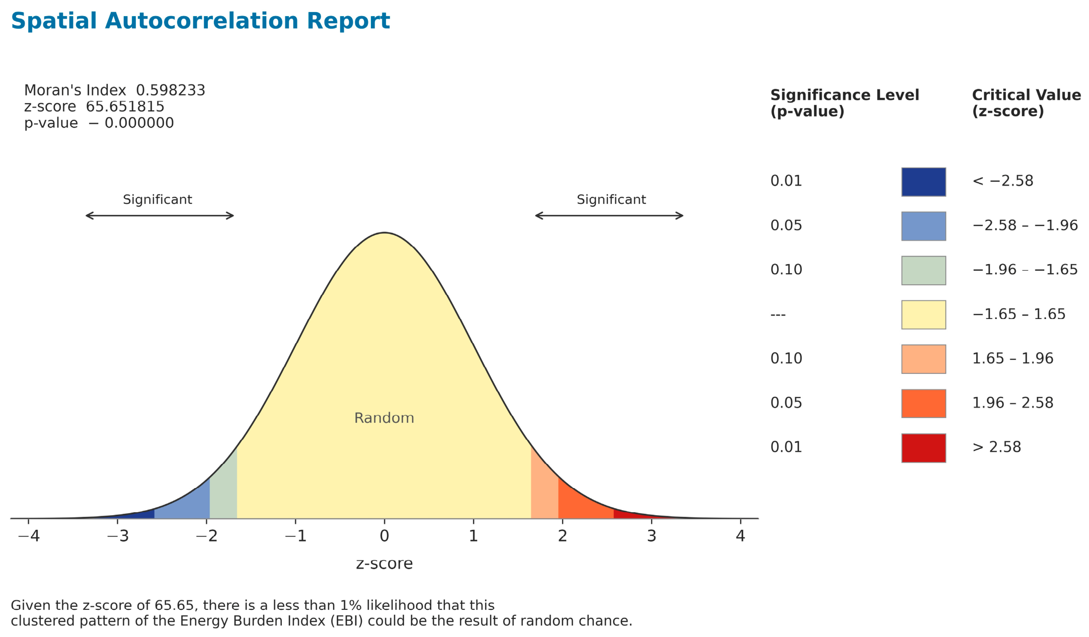
The bell curve output (Figure A1) generated by ArcGIS Pro Spatial Autocorrelation tool shows the observed Moran’s Index of 0.598 positioned in the far-right tail of the distribution (z = 65.65, p < 0.001), well beyond the critical threshold of ±2.58. The red-shaded clustered panel confirms that the spatial pattern of high energy burden across North Carolina census tracts is statistically significant and clustered rather than random or dispersed, validating the use of spatially targeted deployment strategies in this study.
Appendix B
Table A1.
Component technical specifications and size search space.
Table A2.
Controller and dispatch settings.
Table A3.
HOMER Pro economic and optimization parameters.
Solar PV, battery, and converter capacities were optimized continuously using the HOMER Optimizer™ algorithm. The biogas generator search space included three options (25, 63, 100 kW); the optimizer selected 100 kW in all biogas-inclusive configurations, consistent with the community-scale feedstock ceiling (Section 2.3.2). The optimal H2 tank capacity under the resilience constraint (2500 kg) lies within the search space and does not represent the search ceiling (7000 kg), confirming the optimizer was not artificially bounded. Fuel cell and electrolyzer efficiencies are derived from HOMER Pro fuel curve parameters, not directly entered. Biogas combustion CO2 emissions are classified as biogenic under IPCC and EPA accounting conventions and do not affect the 100% renewable fraction reported by HOMER Pro.
Appendix C. Battery State of Charge Calendar Heatmap of All Scenarios
Figure A2 displays hour of day (vertical axis, 0–24 h) versus simulation day (horizontal axis, Days 1–365); color scale indicates SOC (%) from 0% (dark navy) to 100% (light teal). The dark band at Days 355–365 in resilience-constrained panels corresponds to the embedded December solar shortfall period. S1 and S2 are presented under the economic constraint only, as both are infeasible under the 0% capacity-shortage constraint.
Figure A2.
Battery state of charge calendar heatmap: all scenarios, economic (5% shortage) and resilience (0% shortage).
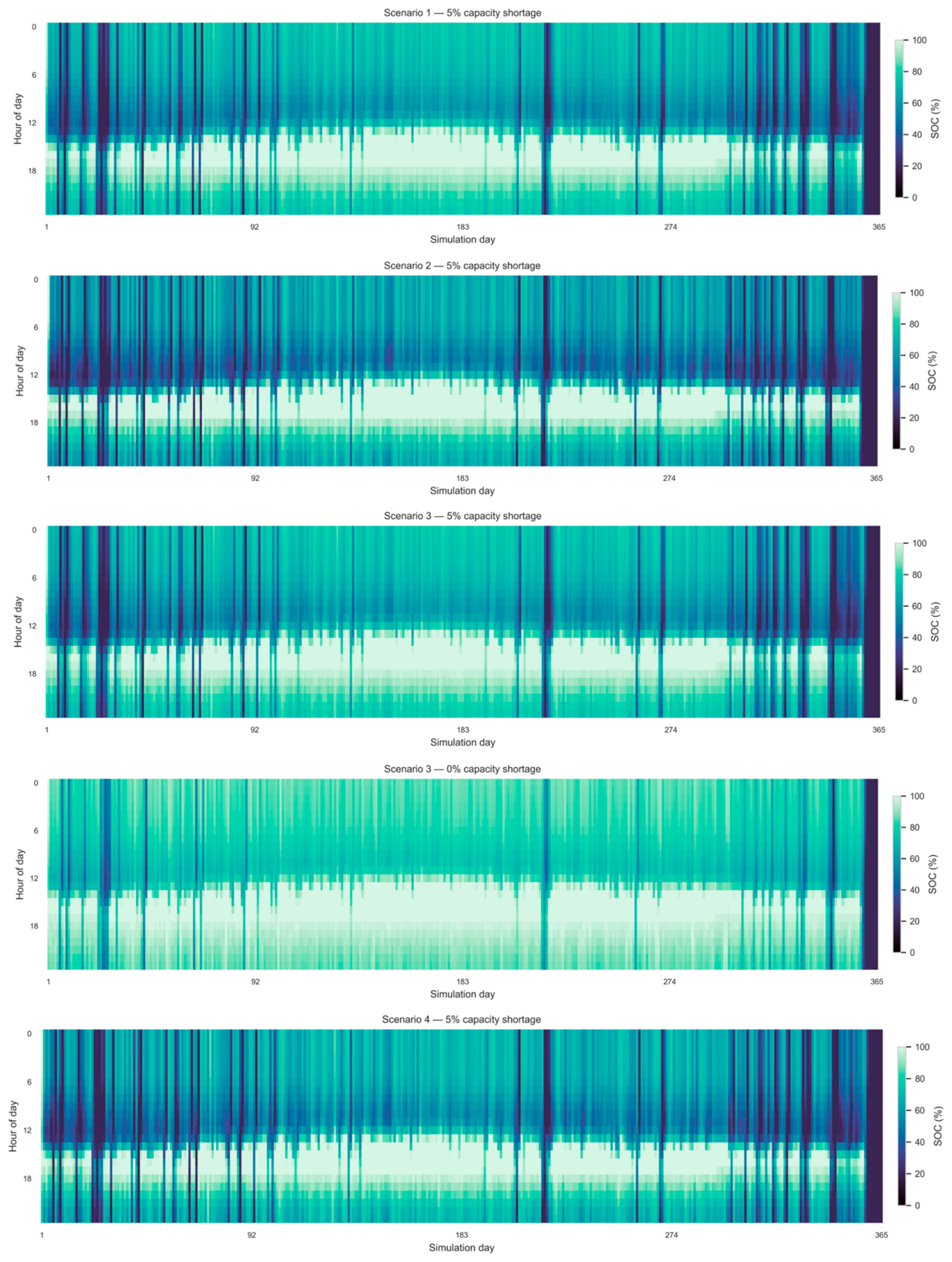
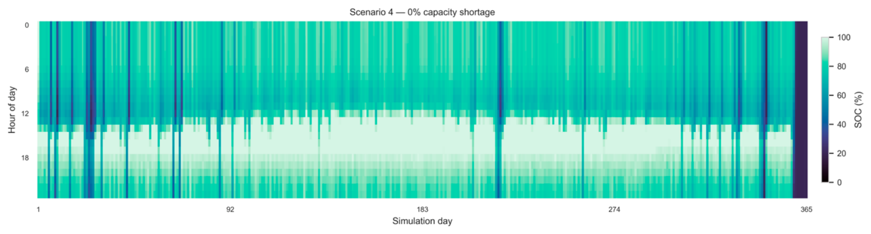
References
- Residential Energy Consumption Survey (RECS)—Energy Information Administration. Available online: https://www.eia.gov/consumption/residential/ (accessed on 20 May 2026).
- How High Are Household Energy Burdens? An Assessment of National and Metropolitan Energy Burdens Across the U.S.|ACEEE. Available online: https://www.aceee.org/research-report/u2006 (accessed on 20 May 2026).
- Low-Income Energy Affordability Data (LEAD) Tool|Department of Energy. Available online: https://www.energy.gov/cmei/scep/low-income-energy-affordability-data-lead-tool (accessed on 18 May 2026).
- Bednar, D.J.; Reames, T.G. Recognition of and response to energy poverty in the United States. Nat. Energy 2020, 5, 432–439. [Google Scholar] [CrossRef] [Scilit]
- Second Annual Clean Energy Convening Highlights Rural North Carolina Strengths-Center for Progressive Reform. Available online: https://progressivereform.org/cpr-blog/2nd-annual-clean-energy-convening-highlights-rural-nc-strengths/ (accessed on 20 May 2026).
- Rural Clean Energy Convening Highlights Need for a Strong ‘Rural Agenda’-Center for Progressive Reform. Available online: https://progressivereform.org/cpr-blog/rural-clean-energy-convening-highlights-need-for-a-strong-rural-agenda/ (accessed on 20 May 2026).
- Drehobl, A.; Ross, L.; Ayala, R.; Zaman, A.; Amann, J. How High Are Household Energy Burdens?An Assessment of National and Metropolitan Energy Burden across the United States SEPTEMBER 2020 How High Are Household Energy Burdens? American Council for an Energy-Efficient Economy: Washington, DC, USA, 2020. [Google Scholar]
- Low-Income Energy Affordability Data-LEAD Tool-2022 Update-Catalog. Available online: https://catalog.data.gov/dataset/low-income-energy-affordability-data-lead-tool-2022-update (accessed on 14 December 2025).
- Irham, A.; Roslan, M.F.; Jern, K.P.; Hannan, M.A.; Mahlia, T.M.I. Hydrogen energy storage integrated grid: A bibliometric analysis for sustainable energy production. Int. J. Hydrogen Energy 2024, 63, 1044–1087. [Google Scholar] [CrossRef] [Scilit]
- Möller, M.C.; Keiner, D.; Breyer, C.; Krauter, S. Techno-economic assessment of a self-sufficient, off-grid solar photovoltaic prosumer system in Germany and Finland using hydrogen seasonal storage. Int. J. Hydrogen Energy 2026, 231, 154456. [Google Scholar] [CrossRef] [Scilit]
- AgSTAR: Biogas Recovery in the Agriculture Sector|US EPA. Available online: https://www.epa.gov/agstar (accessed on 21 May 2026).
- Babatunde, O.M.; Munda, J.L.; Hamam, Y. Hybridized off-grid fuel cell/wind/solar PV/battery for energy generation in a small household: A multi-criteria perspective. Int. J. Hydrogen Energy 2022, 47, 6437–6452. [Google Scholar] [CrossRef] [Scilit]
- HOMER—Microgrid and Hybrid Power Modeling Software. Available online: https://www.homerenergy.com (accessed on 23 February 2026).
- Aktas, I.S. Techno-economic feasibility analysis and optimisation of on/off-grid wind-biogas-CHP hybrid energy system for the electrification of university campus: A case study. Renew. Energy 2024, 237, 121792. [Google Scholar] [CrossRef] [Scilit]
- Larminie, J.; Dicks, A. Fuel Cell Systems Explained, 2nd ed.; John Wiley & Sons Ltd.: Chichester, UK, 2003; pp. 1–406. [Google Scholar] [CrossRef] [Scilit]
- He, M.; Liang, Y.; Lv, C.; Gong, L.; Wu, J.; Liu, L. Numerical simulation and experiment study on the dynamic characteristics of the filling process of cryo-compressed hydrogen storage tanks. Int. J. Hydrogen Energy 2025, 141, 1006–1018. [Google Scholar] [CrossRef] [Scilit]
- Lokar, J.; Virtič, P. The potential for integration of hydrogen for complete energy self-sufficiency in residential buildings with photovoltaic and battery storage systems. Int. J. Hydrogen Energy 2020, 45, 34566–34578. [Google Scholar] [CrossRef] [Scilit]
- Raza, A.; Chen, Y.; Li, M.; Abouzeid, S.I.; Abdelhameed, E.H. Feasibility and optimal size analysis of off grid hybrid AC-DC microgrid system: Case study of El Kharga Oasis, Egypt. J. Energy Storage 2024, 97, 112721. [Google Scholar] [CrossRef] [Scilit]
- Chowdhury, N.; Calais, M.; Shafiullah, G.M. Optimization approaches for renewable microgrid applications with hydrogen and battery energy storage—A comprehensive review. J. Energy Storage 2026, 170, 122744. [Google Scholar] [CrossRef] [Scilit]
- Ghenai, C.; Salameh, T.; Merabet, A. Technico-economic analysis of off grid solar PV/Fuel cell energy system for residential community in desert region. Int. J. Hydrogen Energy 2020, 45, 11460–11470. [Google Scholar] [CrossRef] [Scilit]
- Abdin, Z.; Mérida, W. Hybrid energy systems for off-grid power supply and hydrogen production based on renewable energy: A techno-economic analysis. Energy Convers. Manag. 2019, 196, 1068–1079. [Google Scholar] [CrossRef] [Scilit]
- Nassereddine, M.; Nassreddine, G.; El Arid, A. Hybrid photovoltaic and biogas system for stable power system. Next Energy 2024, 5, 100172. [Google Scholar] [CrossRef] [Scilit]
- Mukhtar, S.; Muhammad, S.; Alyousef, H.A.; Khan, W.; Shah, R.; El-Tantawy, S.A. Enviro-economic and optimal hybrid energy system: Photovoltaic–biogas–hydro–battery system in rural areas of Pakistan. Heliyon 2024, 10, e35182. [Google Scholar] [CrossRef] [Scilit] [PubMed]
- Ennemiri, N.; Berrada, A.; Emrani, A.; Abdelmajid, J.; El Mrabet, R. Optimization of an off-grid PV/biogas/battery hybrid energy system for electrification: A case study in a commercial platform in Morocco. Energy Convers. Manag. X 2024, 21, 100508. [Google Scholar] [CrossRef] [Scilit]
- Tiam Kapen, P.; Medjo Nouadje, B.A.; Chegnimonhan, V.; Tchuen, G.; Tchinda, R. Techno-economic feasibility of a PV/battery/fuel cell/electrolyzer/biogas hybrid system for energy and hydrogen production in the far north region of cameroon by using HOMER pro. Energy Strateg. Rev. 2022, 44, 100988. [Google Scholar] [CrossRef] [Scilit]
- Messaoudi, D.; Settou, N.; Negrou, B.; Settou, B. GIS based multi-criteria decision making for solar hydrogen production sites selection in Algeria. Int. J. Hydrogen Energy 2019, 44, 31808–31831. [Google Scholar] [CrossRef] [Scilit]
- Rezaei, M.; Khalilpour, K.R.; Jahangiri, M. Multi-criteria location identification for wind/solar based hydrogen generation: The case of capital cities of a developing country. Int. J. Hydrogen Energy 2020, 45, 33151–33168. [Google Scholar] [CrossRef] [Scilit]
- Flora, F.M.I. A GIS-based on application of Monte Carlo and multi-criteria decision-making approach for site suitability analysis of solar-hydrogen production: Case of Cameroon. Heliyon 2025, 11, e41541. [Google Scholar] [CrossRef] [Scilit] [PubMed]
- Panteli, M.; Mancarella, P. The grid: Stronger, bigger, smarter?: Presenting a conceptual framework of power system resilience. IEEE Power Energy Mag. 2015, 13, 58–66. [Google Scholar] [CrossRef] [Scilit]
- Zhou, Y.; Panteli, M.; Moreno, R.; Mancarella, P. System-level assessment of reliability and resilience provision from microgrids. Appl. Energy 2018, 230, 374–392. [Google Scholar] [CrossRef] [Scilit]
- Hirsch, A.; Parag, Y.; Guerrero, J. Microgrids: A review of technologies, key drivers, and outstanding issues. Renew. Sustain. Energy Rev. 2018, 90, 402–411. [Google Scholar] [CrossRef] [Scilit]
- Khodaei, A.; Bahramirad, S.; Shahidehpour, M. Microgrid Planning Under Uncertainty. IEEE Trans. Power Syst. 2015, 30, 2417–2425. [Google Scholar] [CrossRef] [Scilit]
- What is GIS?|Geographic Information System Mapping Technology. Available online: https://www.esri.com/en-us/what-is-gis/overview (accessed on 18 May 2026).
- Agriculture, Biogas, Municipal Solid Waste, Wastewater-Anaerobic Digestion Screening Tool|Global Methane Initiative. Available online: https://www.globalmethane.org/resources/details.aspx?resourceid=5170 (accessed on 18 May 2026).
- U.S. Census Bureau. TIGER/Line Shapefiles. Available online: https://www.census.gov/geographies/mapping-files/time-series/geo/tiger-line-file.html (accessed on 18 May 2026).
- Munkhbat, U.; Choi, Y. GIS-based site suitability analysis for solar power systems in Mongolia. Appl. Sci. 2021, 11, 3748. [Google Scholar] [CrossRef] [Scilit]
- Adebimpe, O.A.; Usman, S.O. A GIS-AHP approach for evaluating site suitability for solar power plant: A case study of Ewekoro LGA, Nigeria. Niger. J. Technol. 2022, 41, 680–692. [Google Scholar] [CrossRef] [Scilit]
- Robeson County, NC: Electric Rates From 5 Providers. Available online: https://findenergy.com/nc/robeson-county-electricity/ (accessed on 19 May 2026).
- Dong, H.; Mangino, J.; McAllister, T.A.; Hatfield, J.L.; Johnson, D.E.; Lassey, K.R.; de Lima, M.A.; Romanovskaya, A. Chapter 10 Emissions from Livestock and Manure Management. In 2006 IPCC Guidelines for National Greenhouse Gas Inventories; IGES: Kanagawa, Japan, 2006. [Google Scholar]
- Data USA. Robeson County, North Carolina. Data USA. 2020. Available online: https://datausa.io/profile/geo/robeson-county-nc#demographics (accessed on 17 March 2026).
- Zahan, Z. Anaerobic Co-Digestion of Chicken Litter with Food and Agro-Industrial Wastes/Residues, an Australian Case Study: Use of Carbon-to-Nitrogen Ratio for Substrate Mixing and Semi-Solids Versus Wet Anaerobic Digestion. Ph.D. Thesis, RMIT University, Melbourne, Australia, 2019. [Google Scholar] [CrossRef]
- Poultry Environmental Quality Handbook. Using Litter to Generate Heat and Electricity; University of Georgia: Athens, GA, USA, 2023; Available online: https://peqh.uga.edu/2023/07/using-litter-to-generate-heat-and-electricity/ (accessed on 17 March 2026).
- NSRDB. Available online: https://nsrdb.nlr.gov/ (accessed on 19 May 2026).
- Index|Electricity|2024|ATB|NLR. Available online: https://atb.nrel.gov/electricity/2024/index (accessed on 19 May 2026).
- Chan, V.; Tian, L.; Shah, J.; Wagner, J. Pathways to Commercial Liftoff: Clean Hydrogen; U.S. Department of Energy: Washington, DC, USA, 2023.
- H2A: Hydrogen Analysis Production Models|Hydrogen and Fuel Cells|NLR. Available online: https://www.nlr.gov/hydrogen/h2a-production-models (accessed on 19 May 2026).
- U.S. Department of Energy. Fuel Cell Technologies Fy 2023 Merit Review and Peer Evaluation Report 209|Fuel Cell Technologies-2023 Fuel Cell Technologies Subprogram Overview; HFTO: Washington, DC, USA, 2023.
- IRENA. Renewable Power Generation Costs in 2022. Available online: https://www.irena.org (accessed on 3 May 2026).
- CHP Technologies|US EPA. Available online: https://www.epa.gov/chp/chp-technologies (accessed on 19 May 2026).
- United Nations Environment Programme. Beyond Foundations: Mainstreaming Sustainable Solutions to Cut Emissions from the Buildings Sector; UNEP: Nairobi, Kenya, 2024. [Google Scholar]
- Luta, D.N.; Raji, A.K. Decision-making between a grid extension and a rural renewable off-grid system with hydrogen generation. Int. J. Hydrogen Energy 2018, 43, 9535–9548. [Google Scholar] [CrossRef] [Scilit]
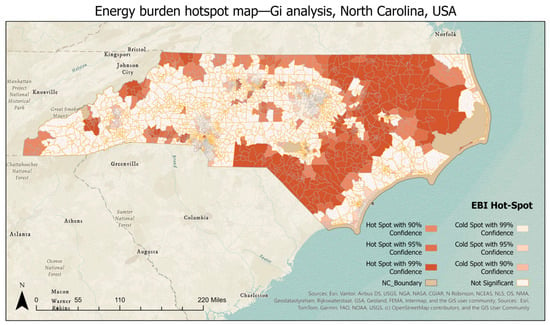
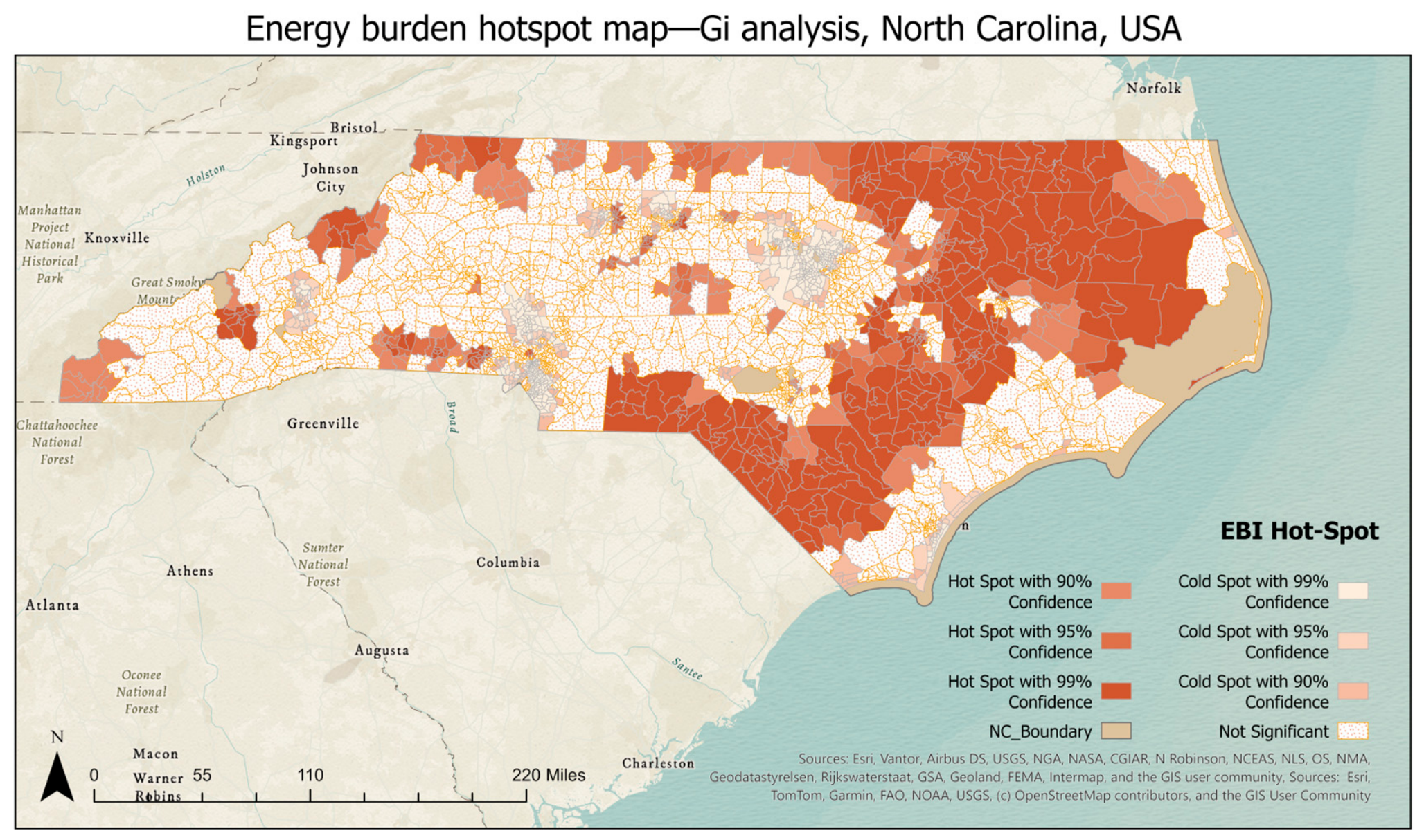
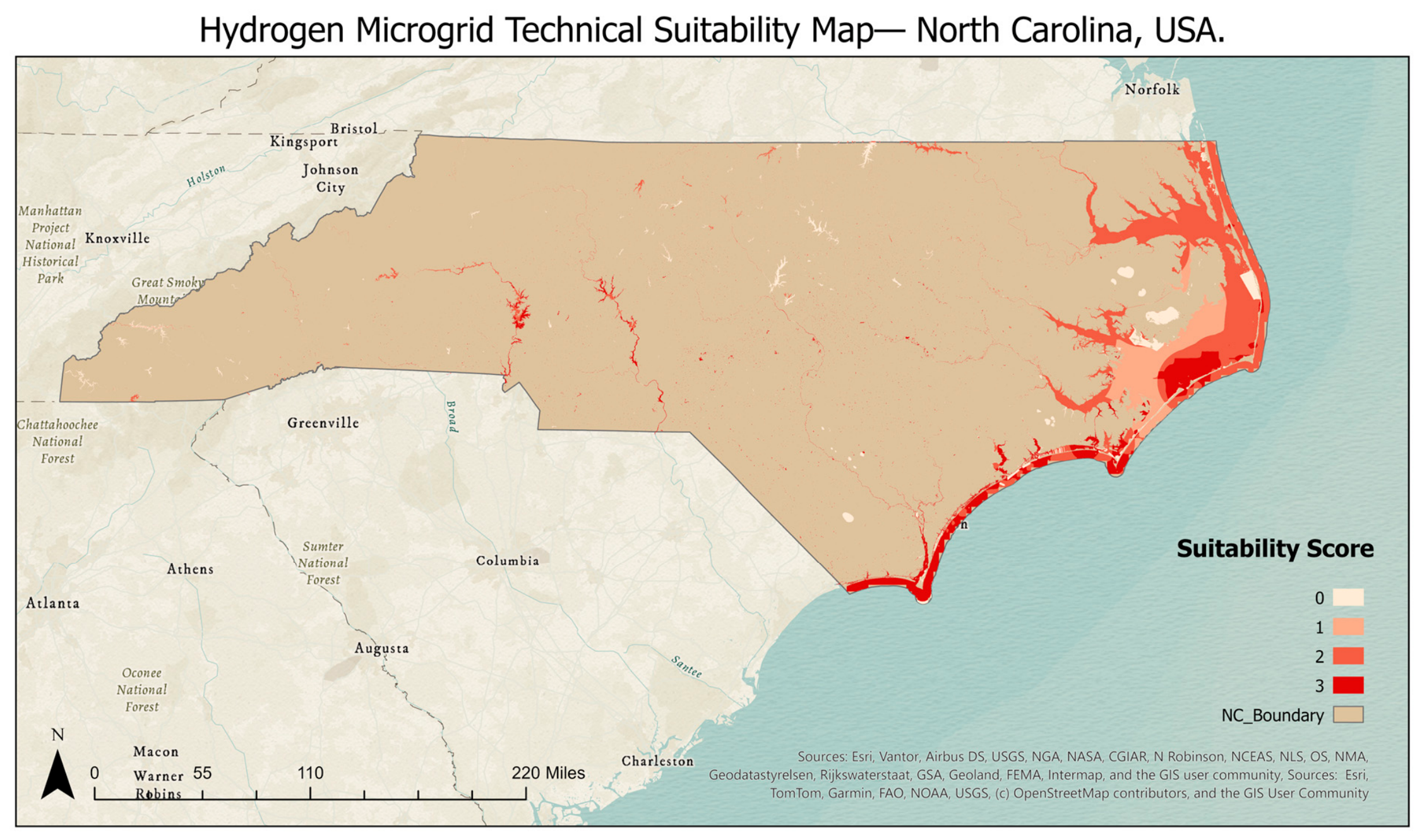
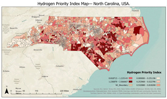
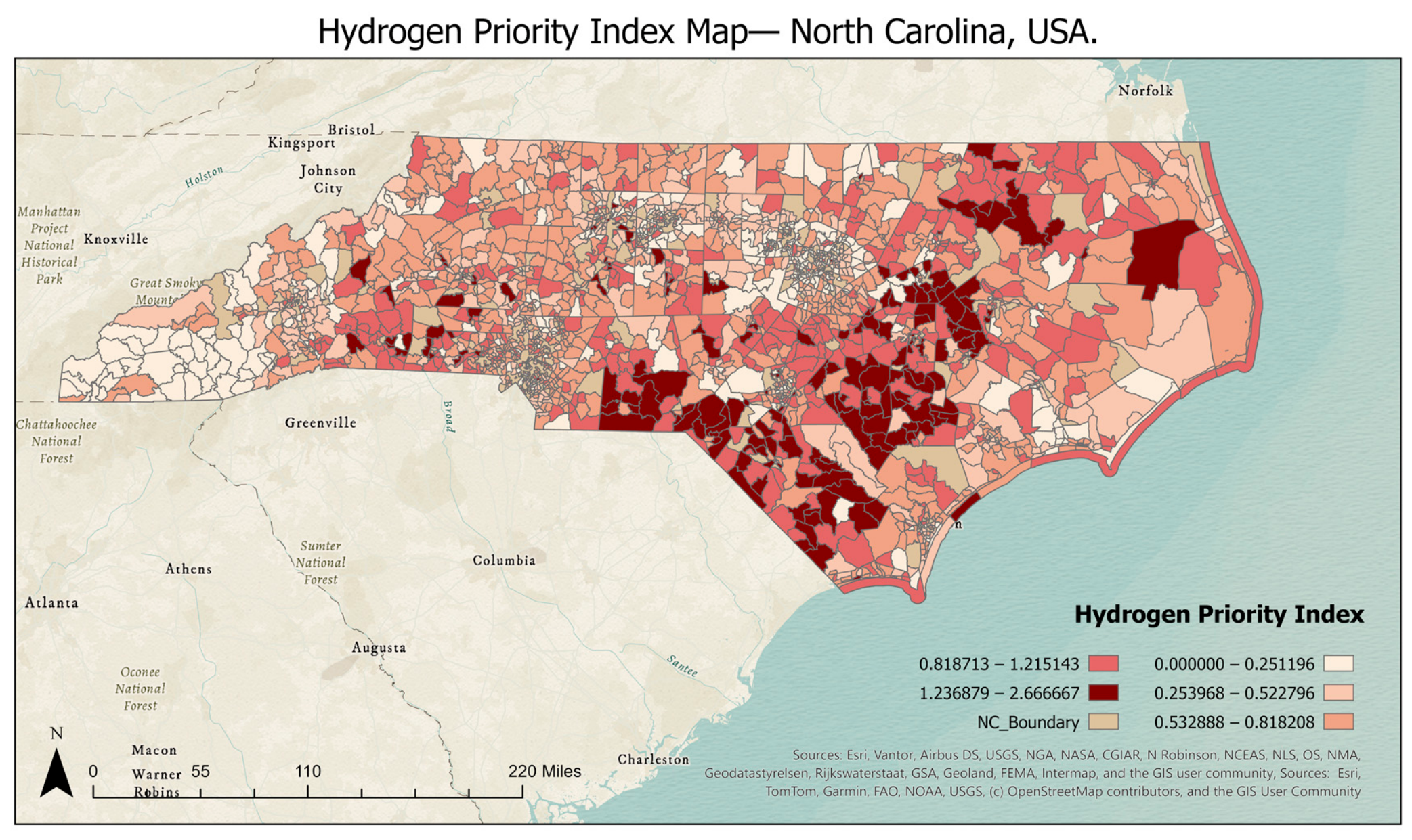
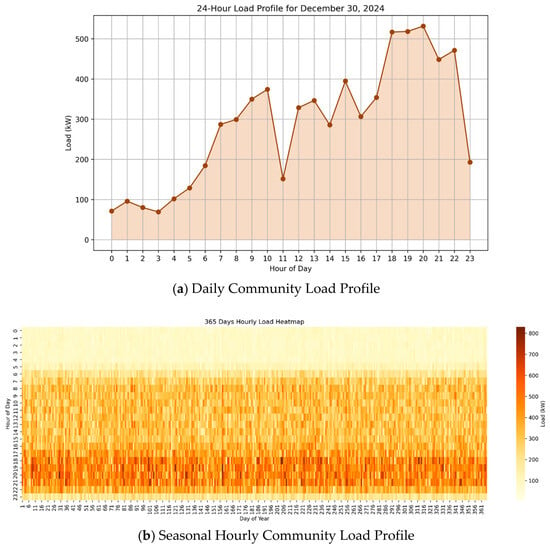
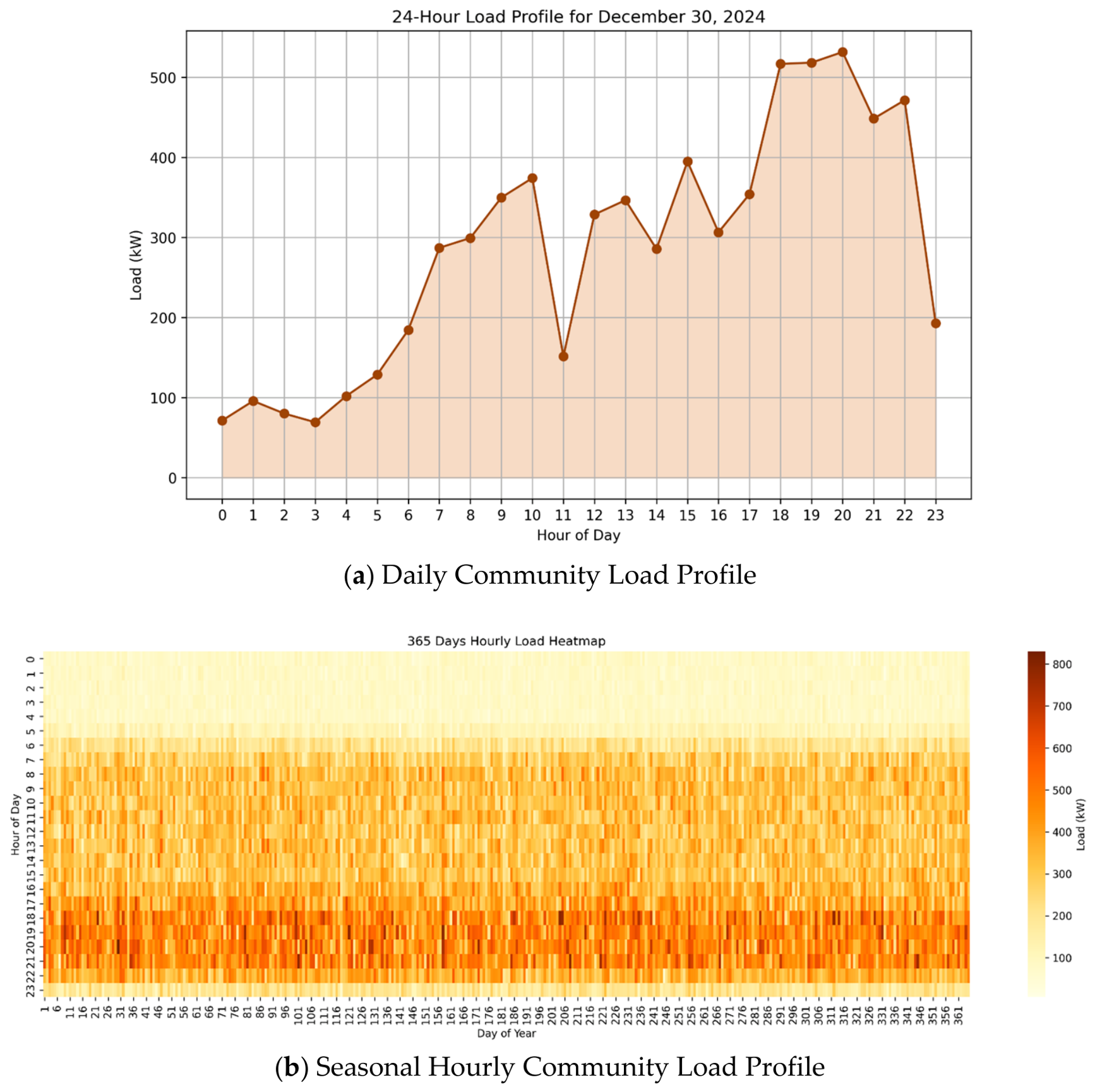
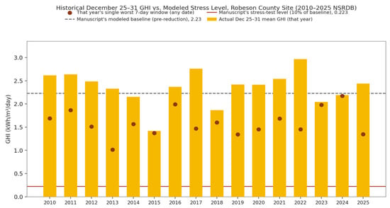
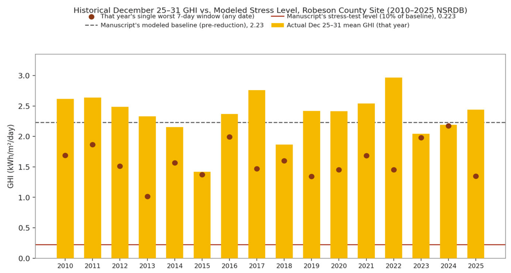
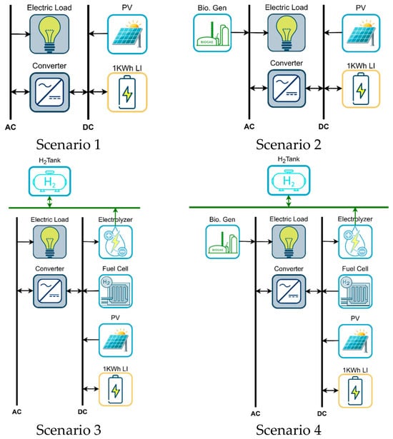
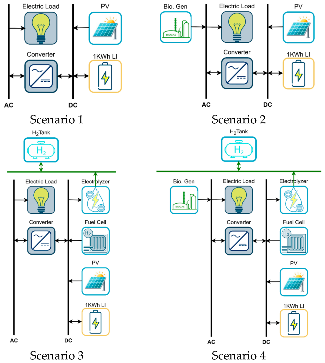
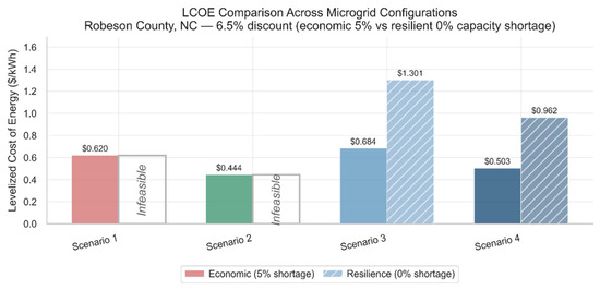
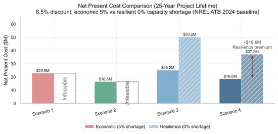
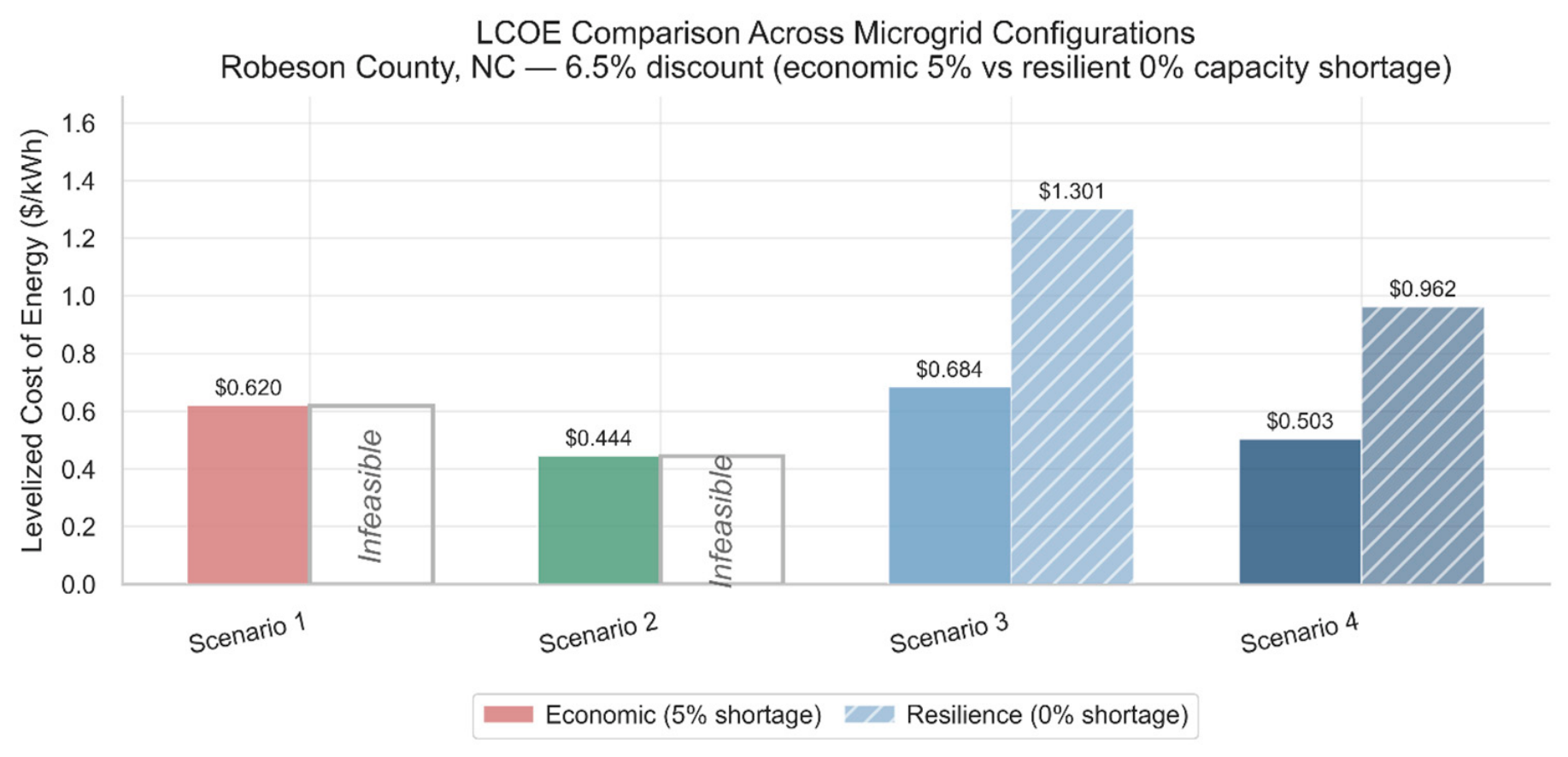
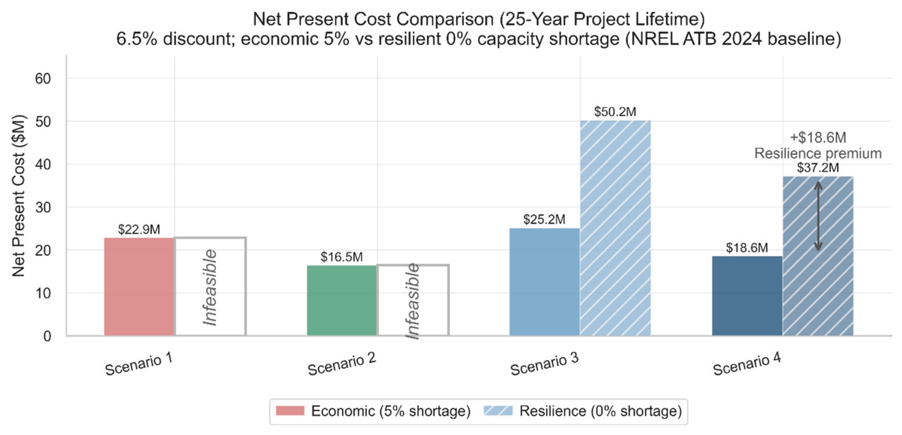
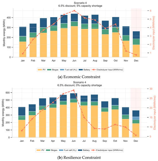
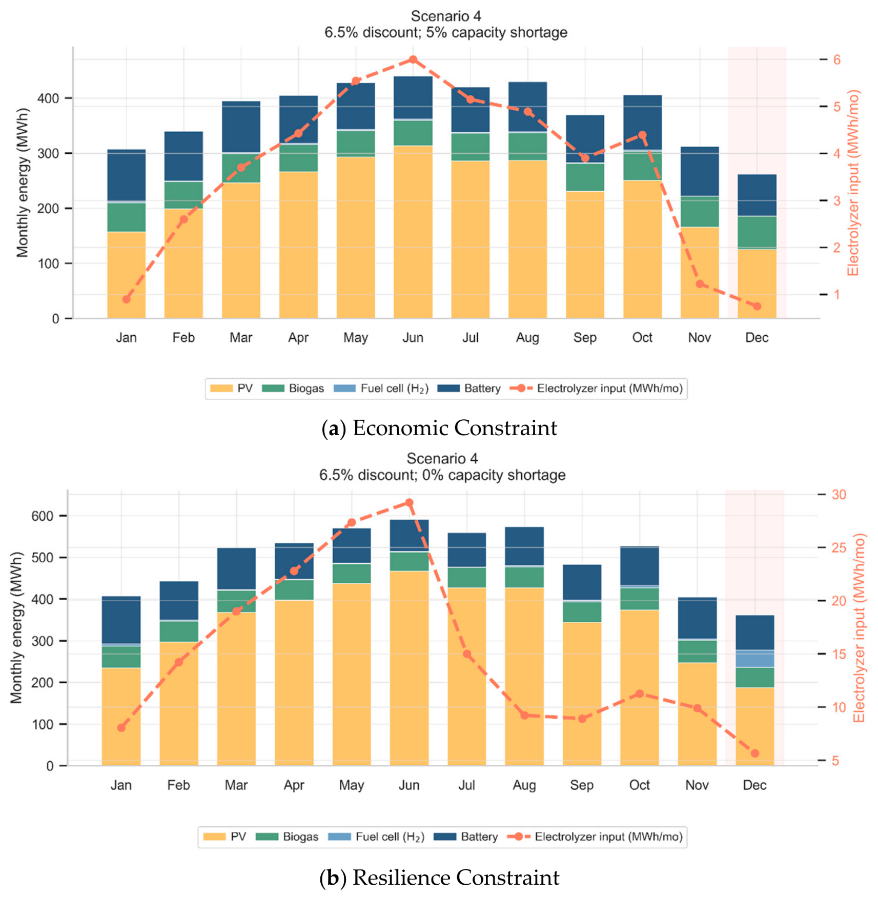
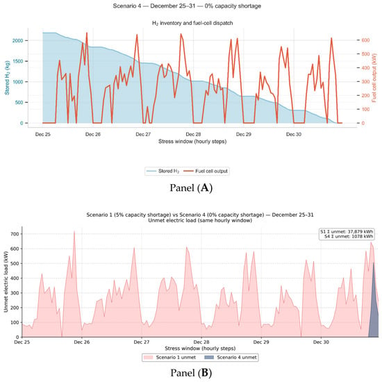
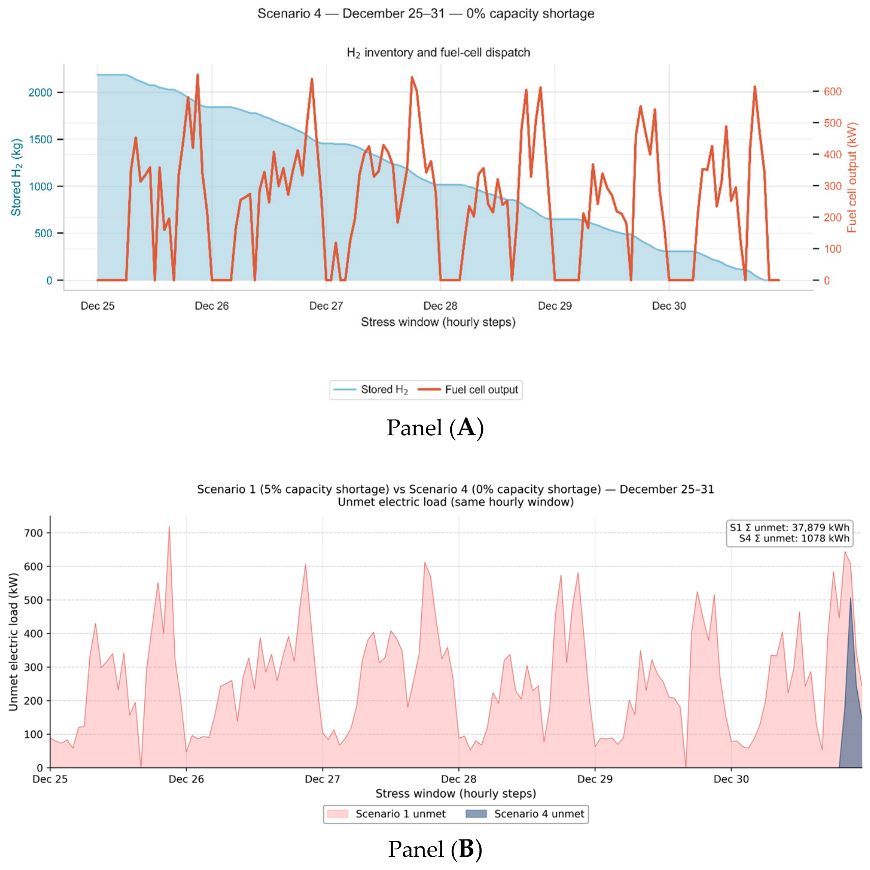
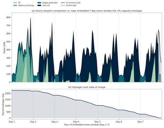
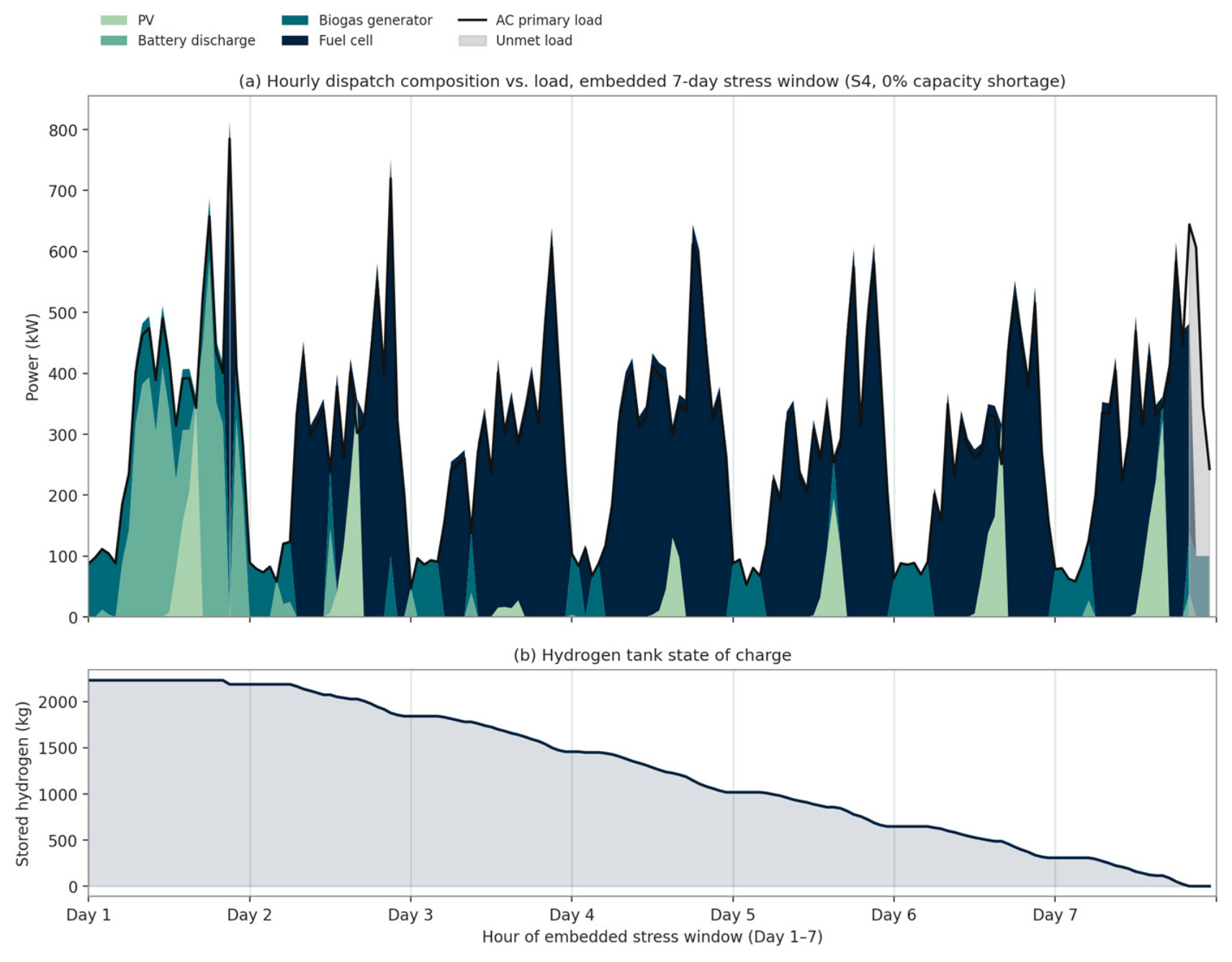
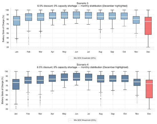
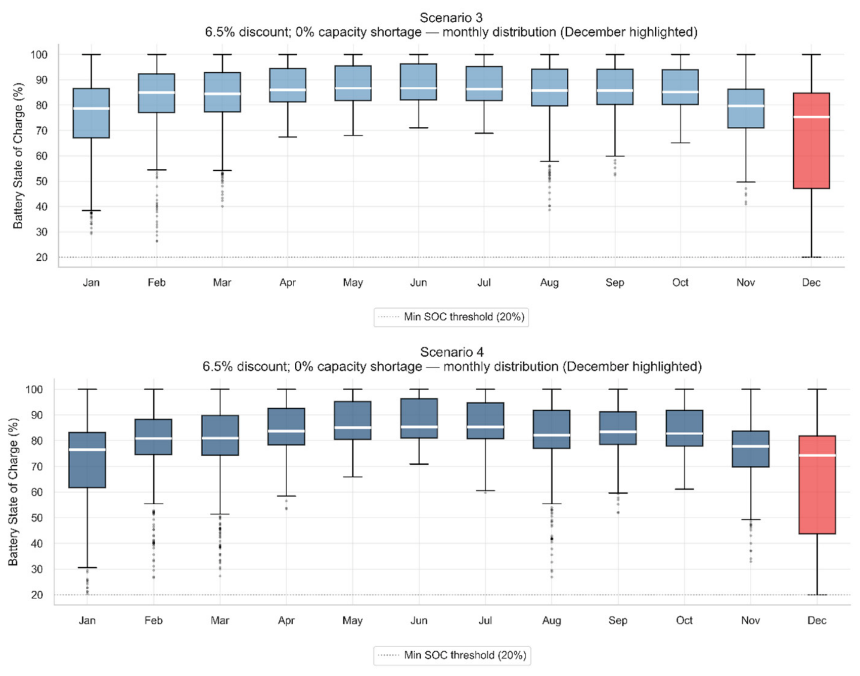
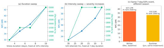
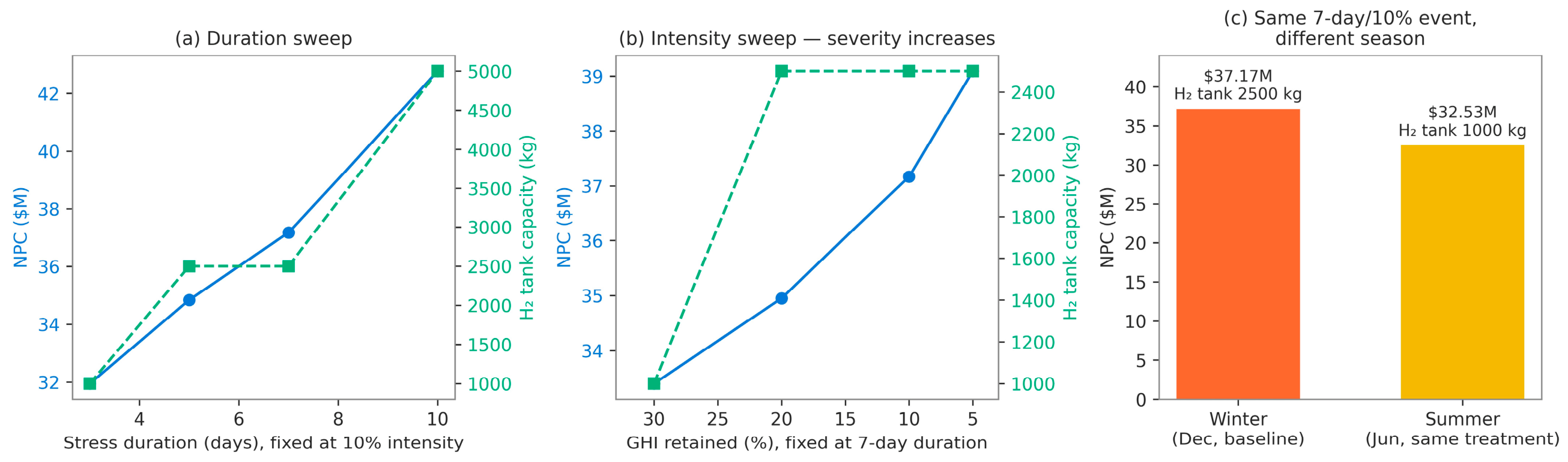
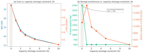
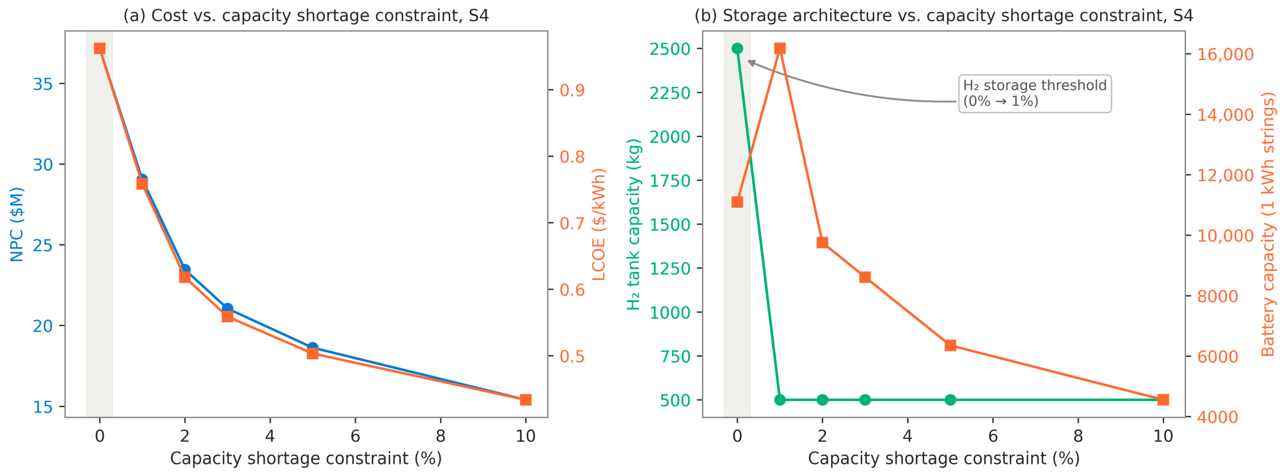
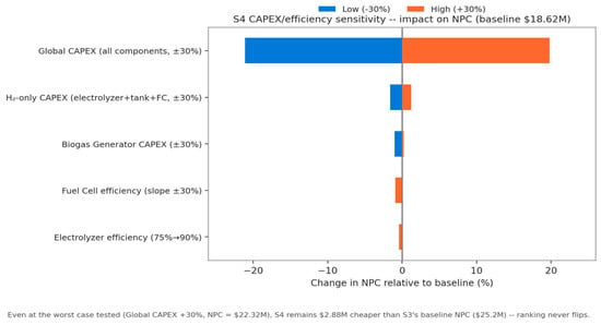
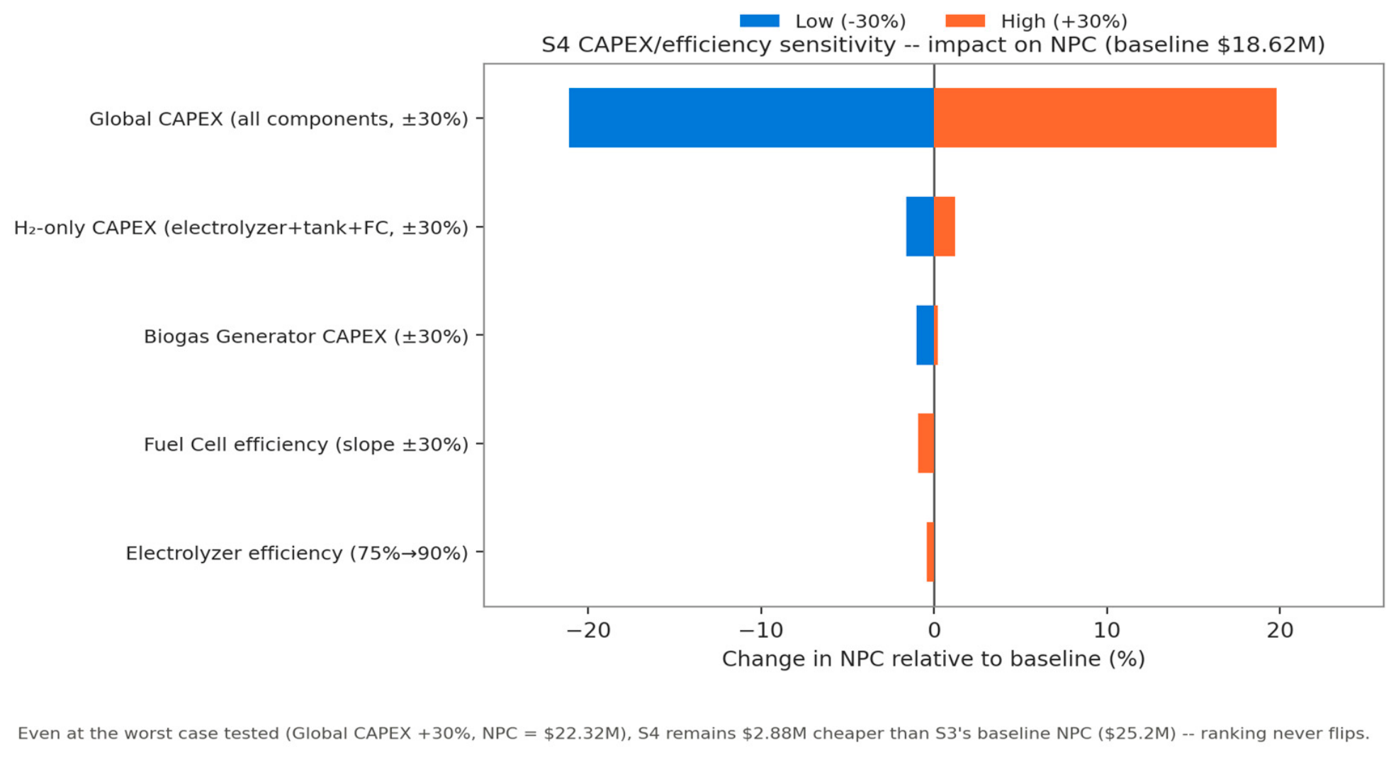

Disclaimer/Publisher’s Note: The statements, opinions and data contained in all publications are solely those of the individual author(s) and contributor(s) and not of MDPI and/or the editor(s). MDPI and/or the editor(s) disclaim responsibility for any injury to people or property resulting from any ideas, methods, instructions or products referred to in the content. |
© 2026 by the authors. Licensee MDPI, Basel, Switzerland. This article is an open access article distributed under the terms and conditions of the Creative Commons Attribution (CC BY) license.