


Abstract
(1) Background: Climate change is reducing the climatic windows in which outdoor sport and physical activity can be safely practised. Yet, it remains unclear whether the resulting population exposure is distributed evenly across countries or is concentrated in countries with higher socio-economic vulnerability. Here, we assess the country-level distribution of population exposure to sport-relevant heat along a projected socio-economic vulnerability gradient. (2) Methods: We assess a screening-level, population-based proxy of sport-relevant heat exposure, defined by residents living in grid cells experiencing specified afternoon WBGT exceedance frequencies. We first quantify a population exposure burden by combining reconstructed afternoon wet-bulb globe temperature (WBGT) exceedance frequencies from bias-corrected CMIP6 projections (NEX-GDDP, five-model ensemble) with SSP-consistent gridded population. The resulting grid-cell exposure burden, expressed in person-days yr−1, is aggregated to the country level. Countries are then ranked using a published national socio-economic vulnerability index (GVI), and the distribution of the exposure burden along this vulnerability gradient is quantified using a population-weighted concentration index (CI). The GVI is used as the ranking variable and is not incorporated into a multiplicative vulnerability-weighted risk metric. Two internally coherent futures (SSP1-2.6 and SSP2-4.5, each paired with its corresponding socio-economic pathway) are evaluated at mid-century (2055) and late century (2085). (3) Results: The population exposure burden is concentrated in more vulnerable countries in all scenario–horizon–threshold combinations (CI > 0; 0.09–0.25). Under SSP1-2.6 at mid-century, the five-model mean CI showed a descriptive increase from 0.17 for WBGT ≥ 28 °C to 0.25 for WBGT ≥ 32 °C, although the 95% paired hierarchical-bootstrap interval for the 32-minus-28 °C contrast included zero. By 2085, about 4.11 billion people live in cells experiencing at least 30 days yr−1 with WBGT ≥ 32 °C under SSP2-4.5, compared with 2.14 billion under SSP1-2.6. (4) Conclusions: The results identify projected between-country inequalities in resident population exposure to sport-relevant heat conditions; they do not quantify actual sport participation, athlete exposure or health outcomes. The comparison between SSP1-2.6 and SSP2-4.5 further shows substantial differences in both climatic hazard and population exposure between these two integrated climate–demographic–socio-economic futures.
1. Introduction
Heat is a first-order constraint on outdoor sport and physical activity. Elevated air temperature and humidity impair thermoregulation, degrade performance and, beyond critical thresholds, become life-threatening: weather conditions measurably slow endurance events [1], heatwaves strain the cardiovascular system [2], and exertional heat illness remains a recurrent cause of death among athletes [3], and major sporting events are increasingly planned around extreme-heat risk for athletes and spectators alike [4,5]. As the climate warms, the conditions under which outdoor sport can be safely practised are therefore being eroded—not as an occasional disruption, but as a progressively structural feature of the sporting calendar.
To represent this combined thermal load, the wet-bulb globe temperature (WBGT) has become the reference index in occupational, military and athletic guidelines, because it integrates temperature, humidity, radiation and wind into a single operationally meaningful quantity [6]. WBGT underpins the heat-policy thresholds of major sport federations, which escalate from activity modification to outright suspension as conditions worsen, and the index responds differently in hot–dry versus warm–humid environments, so that the same air temperature can carry very different physiological cost [7]; beyond a point, heat stress becomes uncompensable even for fit individuals exercising at moderate intensity [8]. Crucially, WBGT-based constraints are projected to expand markedly under future warming, increasing the frequency of outdoor conditions associated with substantial physiological heat stress across large parts of the globe [9,10].
A large body of literature has quantified how many people will be exposed to extreme heat as the climate warms. Global assessments project a rapid rise in humid-heat stress [11], sharp increases in population exposure in the United States [12] and Africa [13], and—most strikingly—that a majority of the urban world will face dangerous heat within decades [14]. These studies establish the magnitude of the exposed population, but they treat that population as an undifferentiated total: they answer “how many”, not “who”.
Yet, exposure to heat is not borne equally. At the city scale, a now-substantial body of work shows that heat falls disproportionately on disadvantaged populations: urban heat-island intensity is systematically higher in lower-income and historically marginalised neighbourhoods [15,16], extreme humid-heat events disproportionately affect the most exposed communities [17], and exposure rises fastest for demographically vulnerable groups such as older adults [18]. This unequal distribution has been framed as a matter of climate justice and human rights [19]. At the international scale, the capacity to cope with such hazards is itself unevenly distributed, and is captured by national-level determinants of vulnerability and adaptive capacity [20,21]. To date, however, this distributional lens has been applied to mortality, labour and urban heat—not to the loss of safe conditions for sport and outdoor physical activity, and not at the global, country-resolved scale.
The intersection of sport, heat and climate projections remains comparatively sparse, and where it exists it has focused on where activity should be located: recent work asks where major sporting events should be held under global warming, using WBGT from downscaled CMIP6 projections [22]. That question is logically prior to, but distinct from, the one we pose here. We do not ask where a single event should go; we ask how the emerging burden of sport-relevant heat is distributed across countries of differing socio-economic vulnerability, and whether that distribution is equitable. In other words, we move from the magnitude of exposure to its concentration along the vulnerability gradient.
Importantly, the sport lens used here is population-based rather than event- or athlete-based. We do not estimate the realised exposure of elite athletes, organised competitions or specific sport calendars. Instead, we quantify the resident population potentially exposed to climatic conditions that constrain safe outdoor sport and physical activity, using WBGT thresholds that are operationally meaningful for heat management in outdoor exercise. This distinction matters for equity: in countries with lower adaptive capacity, the same heat-stress hazard may translate more directly into lost opportunities for school sport, youth sport, community sport and everyday physical activity, because protective infrastructure, medical supervision, shaded or indoor facilities, and scheduling flexibility are less widely available.
Existing research has examined climate change and physical activity broadly [23], the climatic suitability of major sporting events [22], occupational heat and work capacity [10], and the implications and management of extreme heat for school-based sport and physical activity [24,25]. The physiological basis and sport-specific consequences of exercising in the heat are also well established [26].
A separate body of literature has documented international and subnational inequalities in heat exposure, primarily in relation to health, labour and urban environments [14,15,16,17]. These research strands provide the physiological, operational and distributional foundations for the present analysis, but they do not directly quantify the future country-level distribution of a population-based sport-relevant WBGT exposure burden along a projected socio-economic vulnerability gradient. The present study connects this literature rather than claiming to establish an entirely new field.
Here we combine sport-relevant afternoon WBGT exceedance from bias-corrected CMIP6 projections with SSP-consistent gridded population to quantify a population exposure burden in person-days per year. We then evaluate how this burden is distributed across countries ranked by a published, externally validated national socio-economic vulnerability index. Working at country level under two internally coherent Shared Socio-Economic Pathways and two future horizons, we ask three questions. First, is the population exposure burden concentrated in countries with higher projected socio-economic vulnerability, and by how much? Second, does the concentration of exposure vary across increasingly severe WBGT thresholds? Third, how do the joint patterns of climatic exposure and projected vulnerability differ between the two integrated SSP futures? By answering these, we provide a transparent, reproducible and equity-aware basis for adaptation planning in sport and outdoor physical activity.
2. Materials and Methods
2.1. Overview: Population Exposure Assessed Along a Socio-Economic Vulnerability Gradient
We quantify the distribution of sport-relevant heat exposure through a two-stage analytical framework. First, the climatic hazard is represented by the annual frequency of afternoon wet-bulb globe temperature (WBGT) threshold exceedance derived from bias-corrected CMIP6 projections. At the grid-cell level, this hazard is combined with the resident population exposed to that hazard. The resulting product, expressed in person-days per year, represents the population exposure burden:
where is the resident population in grid cell i, is the annual mean number of days exceeding the selected WBGT threshold in climate model m, and is the corresponding model-specific population exposure burden.
Second, the grid-cell exposure burden is aggregated to the country level and analysed along a national socio-economic vulnerability gradient using the Global Vulnerability Index (GVI). The GVI is not multiplied by either the climatic hazard or the population and therefore does not constitute part of a vulnerability-weighted risk metric. Instead, it is used exclusively as the country-ranking variable in the concentration analysis.
Accordingly, this study explicitly distinguishes between: (i) climatic hazard frequency (days yr−1); (ii) population exposure burden (person-days yr−1); (iii) population-weighted per capita exposure (days person−1 yr−1); and (iv) projected national socio-economic vulnerability, represented by the GVI. The analysis therefore quantifies the distribution of climatic exposure burden across projected vulnerability levels, rather than estimating vulnerability-weighted risk, health impacts, realised sport participation, or adaptive capacity loss.
Two internally consistent future pathways (SSP1–2.6 and SSP2–4.5) are analysed for two time horizons (2055 and 2085). The complete processing sequence, from the model-specific climate variables and WBGT reconstruction to population overlay, country aggregation, vulnerability ranking, concentration analysis and ensemble summaries, is presented schematically in Supplementary Figure S4.
2.2. Climate Hazard
Heat-stress exposure was quantified using outdoor Wet-Bulb Globe Temperature (WBGT), a biometeorological index widely recommended for occupational and sport heat-risk assessment [27,28]. Following the methodological approach applied by Sawadogo et al. [22] for football climate-risk assessment, outdoor WBGT was calculated using the standard outdoor-sun formulation
where is the natural wet-bulb temperature, the black-globe temperature, and the near-surface air temperature.
Daily meteorological variables were obtained from the bias-corrected, statistically downscaled NASA NEX-GDDP-CMIP6 archive at 0.25° spatial resolution [29]. The required variables were daily maximum and minimum air temperature (tasmax, tasmin), daily mean relative humidity (hurs) and surface downwelling shortwave radiation (rsds).
Because CMIP6 models do not directly provide either or , both variables were reconstructed from these meteorological fields. Natural wet-bulb temperature was estimated using the analytical psychrometric approximation proposed by Stull [30], whose mean error is below approximately 0.3 °C under standard atmospheric conditions.
Daily mean relative humidity was first adjusted to be physically consistent with the daily temperature maximum following the procedure described in Sawadogo et al. [22]. Daily vapour pressure was estimated from daily mean temperature and relative humidity using the Tetens saturation–vapour–pressure relationship and subsequently converted to the relative humidity corresponding to the daily maximum temperature. This procedure approximates afternoon humidity while preserving atmospheric moisture content.
Black-globe temperature was estimated using the empirical regression of Hajizadeh et al. [31]:
where is surface downwelling shortwave radiation (W m−2), is relative humidity (%), and is expressed in °C. This empirical formulation reproduces the radiative component of outdoor heat stress while remaining computationally suitable for large-scale climate projections.
The resulting WBGT therefore represents outdoor-sun conditions and accounts for the combined influence of air temperature, humidity and solar radiation. Wind effects are represented implicitly through the empirical calibration of the globe temperature regression rather than by explicit solution of the complete radiative-convective energy balance.
Five CMIP6 climate models were analysed independently: GFDL-ESM4, IPSL-CM6A-LR, MPI-ESM1-2-HR, MRI-ESM2-0 and UKESM1-0-LL. Afternoon WBGT was reconstructed separately for each climate model from its own meteorological fields. Threshold exceedance was then computed independently for each model before any ensemble aggregation.
For each WBGT threshold, the climatic hazard in grid cell i and model m was defined as
where is the monthly number of days exceeding the selected WBGT threshold during month t. Thus, represents the annual mean exceedance frequency (days yr−1) over the corresponding 30-year climatological period.
Three mutually exclusive WBGT classes (28–30, 30–32 and ≥32 °C) were first calculated separately for every climate model. Cumulative exceedance frequencies for WBGT ≥ 28 °C and WBGT ≥ 30 °C were subsequently obtained by summing the appropriate classes. No threshold was ever applied to an ensemble-mean WBGT field.
The ensmean product used elsewhere in the workflow is simply the arithmetic mean of the final model-specific exceedance-frequency fields. Country exposure burdens, concentration curves and concentration indices were likewise calculated independently for each climate model before ensemble summary statistics were derived.
The large-scale plausibility of the underlying daily heat-stress reconstruction was assessed in an independent comparison of NEX-GDDP-CMIP6 climatologies with ERA5 over 1991–2020 [32]. In that evaluation, the related daily-resolution shade-WBGT reconstruction showed an area-weighted mean bias of +0.78 °C, a root-mean-square error of 1.59 °C, a mean absolute error of 1.19 °C and a spatial correlation of 0.994. Residual differences were spatially structured, with larger deviations in regions characterised by strong humidity gradients and complex tropical or subtropical near-surface climates, whereas biases were generally weaker and spatially smoother at middle and high latitudes.
These statistics provide an external cross-product evaluation of the NEX-GDDP-CMIP6 inputs and of the broad spatial representation of heat-stress conditions. They are not a direct validation of the exact outdoor-sun formulation used here, because the present calculation adds the empirical black-globe temperature regression of Hajizadeh et al. [31]. A global direct validation against observed outdoor WBGT was not possible because co-located measurements of air temperature, humidity, radiation and black-globe temperature are not available with sufficient global coverage.
Hazard was evaluated over two 30-year climatological windows, 2041–2070 and 2071–2100, referred to throughout the manuscript by their representative central years 2055 and 2085. Three WBGT severity thresholds were considered: ≥28, ≥30 and ≥32 °C. These thresholds correspond to commonly used operational heat-management levels in sport and occupational guidance and are interpreted as harmonised environmental severity classes rather than universal physiological limits applicable to all sports, activities or individuals.
2.3. Sport Relevance of the WBGT Thresholds
WBGT is used here as an environmental severity metric for outdoor sport and physical activity, not as a direct prediction of individual heat strain. Its relevance comes from its operational use in sport heat policies, because it integrates air temperature, humidity, radiation and wind into a single index that can be linked to activity modification, additional rest, cooling strategies, rescheduling or cancellation [5,6,33]. Recent reviews of International Federation policies show that WBGT, or closely related thermal indices, are widely used to assess heat-related risk in outdoor and endurance sports [33]. In professional football, for example, proposed heat-protection guidance recommends cooling breaks above WBGT 26 °C and delay or postponement of matches above WBGT 28 °C [34]. Other sport organisations use comparable WBGT-based triggers for operational mitigation, such as mandatory hydration breaks around WBGT 30 °C in collegiate football/soccer contexts [35].
The thresholds used in this study should therefore be interpreted as harmonised severity levels rather than universal medical cut-offs. WBGT ≥ 28 °C marks conditions under which heat management becomes operationally relevant in several sport policies; WBGT ≥ 30 °C represents a high heat-stress level where substantial modification of outdoor activity may be required; and WBGT ≥ 32 °C is used as a severe, suspension-level screening threshold for many outdoor activities. This harmonised threshold set is appropriate for a global country-level assessment, but it does not imply that the same physiological limit applies to all sports, ages, acclimatisation states or environmental contexts. Indeed, sport-specific modelling indicates that upper thermal thresholds may differ substantially across activities and may need to be revised for some sports [36]. The purpose of the thresholds here is therefore to compare the geographical and socio-economic concentration of increasingly severe sport-relevant heat, not to prescribe event-specific cancellation rules.
Throughout this study, “sport-relevant heat exposure” refers to a screening-level, population-based proxy defined by residence in grid cells experiencing specified afternoon WBGT exceedance frequencies. It does not represent realised exposure during sport or physical activity and does not identify an activity-defined population.
2.4. Population Exposure
Population exposure was quantified using SSP-consistent gridded population projections provided as population counts on an approximately 1 km grid [37]. The population pathway was matched to the corresponding climatic pathway: SSP1 population was paired with SSP1-2.6, whereas SSP2 population was paired with SSP2-4.5. Population was sampled at the central year of each climatic window, namely 2055 and 2085, so that climatic and demographic conditions co-evolve consistently within each integrated future.
Population counts were aggregated from their native approximately 1 km grid to the 0.25° climate grid by summation, following the procedure described in Section 2.6. The climatic hazard was not spatially downscaled, and no sub-grid climatic information was inferred from the finer-resolution population data.
For each scenario and horizon, the resulting exposure layer provides the resident population assigned to each 0.25° grid cell i. This population is spatially co-located with the model-specific hazard . The same population field was used for all five climate models within a given SSP–horizon combination. Consequently, differences among model-specific exposure estimates within the same integrated future arise from differences in the projected climatic hazard rather than from differences in population.
The directly quantified outcome is therefore the number of residents living in grid cells with specified WBGT exceedance frequencies, together with the corresponding person-day burden and population-weighted per capita exposure. No information on actual sport participation, activity timing, duration, intensity or adaptation is used in the calculation.
2.5. Socio-Economic Vulnerability
Socio-economic vulnerability is characterised using the Global Vulnerability Index (GVI) Projection Database [38]. The database provides national projections of the GVI in five-year intervals under SSP1, SSP2 and SSP3. The index, reported as pgvi, ranges from 0 to 100, with higher values indicating greater socio-economic vulnerability.
The projected index builds on the Global Data Lab Vulnerability Index developed by Smits and Huisman [39]. The GVI is designed to represent the human and societal components of vulnerability to climate change, natural hazards and other shocks. It does not include the physical climatic hazard, geographical exposure, built-environment characteristics or other biophysical components. The original GVI combines eleven indicators representing seven major dimensions of socio-economic vulnerability: the economy, education, gender, health, infrastructure, governance and demography.
The GVI formula was derived using principal component analysis applied to a dataset covering 162 countries over the period 2015–2020. The first principal component explains 66.4% of the variance among the underlying indicators, and all indicators contribute substantially to the resulting component [39]. The component score was subsequently transformed and reversed to produce the final 0–100 scale, on which higher scores denote higher vulnerability.
The index has also undergone external and internal validation. At the national level, the 2020 GVI is strongly associated with established measures of vulnerability and adaptive capacity. Reported Pearson correlations include 0.89 with the vulnerability component of ND-GAIN, 0.89 with its adaptive capacity component, 0.84 with the INFORM index and 0.93 with the INFORM coping capacity component. The GVI is also correlated with the vulnerability (), susceptibility () and adaptive capacity () components of the World Risk Index [39]. In addition, reduced GVI specifications obtained by removing individual indicators correlate above 0.99 with the complete index, indicating that the index is not driven by a single underlying indicator.
We deliberately use this independently developed and validated index rather than constructing an ad hoc vulnerability metric specifically for the present analysis. For SSP1-2.6, we use the corresponding SSP1 GVI projections; for SSP2-4.5, we use the SSP2 projections. National GVI values are selected for 2055 and 2085, matching the central years of the two climatic periods.
Because the GVI is available at national resolution, it is joined to the analysis only after the grid-cell population exposure burden has been aggregated to countries. It is never projected onto the climate grid and is not multiplied by either the climatic hazard or the population exposure burden. The GVI is used exclusively to order countries from lower to higher projected socio-economic vulnerability for the concentration analysis. Consequently, although the climatic hazard and exposure burden are calculated independently of the GVI, the resulting concentration curves and concentration indices remain conditional on the country ranking generated by this vulnerability measure.
Sensitivity to temporal and SSP-specific changes in the national GVI ranking is assessed separately by recalculating the concentration indices using a common ranking fixed at the 2020 baseline, as described in Section 2.8.
Because the GVI is measured at national resolution, all residents of a country inherit the same vulnerability value. The concentration analysis therefore measures between-country inequality in exposure along a national vulnerability ranking. It does not capture within-country differences in vulnerability or exposure, and the repeated individual ranks implied by the national grouping are treated explicitly through population-weighted fractional ranks, as described in Section 2.7.
2.6. Population Exposure Burden and Country Aggregation
The grid-cell population exposure burden defined in Section 2.1 was calculated and aggregated independently for each climate model. The SSP-consistent population data, provided as counts on an approximately 1 km grid, were first aggregated to the 0.25° WBGT grid. Each 1 km population pixel was assigned to the climate grid cell containing its centre, and all population counts assigned to the same climate cell were summed. The WBGT field was not spatially downscaled, and no sub-grid climatic information was inferred.
Country boundaries from Natural Earth were rasterised directly onto the 0.25° climate grid using the ADM0_A3 country codes. Rasterisation was performed using the standard centre-based rule (all_touched = FALSE): a climate grid cell was assigned to a country when its centre fell within the corresponding national polygon. Each valid climate grid cell was therefore assigned to at most one country. Neither fractional-area nor fractional-population allocation between neighbouring countries was applied. As a consequence, small islands, narrow coastal territories and fragmented archipelagos may be imperfectly represented at 0.25° resolution.
Population was not clipped by national boundaries before its aggregation to the climatic grid. Country attribution was applied after aggregation to the 0.25° grid. For coastal and international-border cells, the complete aggregated population and associated exposure burden were assigned to the single country containing the cell centre. Cells whose centres did not fall within a valid national polygon remained unassigned and did not contribute to country-level estimates.
For climate model m, the grid-cell population exposure burden was
where is the resident population assigned to grid cell i and is the model-specific annual mean frequency of exceedance of the selected WBGT threshold. The burden is expressed in person-days yr−1. Scenario, horizon and threshold indices are omitted from the notation for readability.
The national population exposure burden was then calculated as
where is the total population exposure burden in country c for climate model m (person-days yr−1).
The corresponding population-weighted per capita exposure was calculated as
where is the model-specific average annual exposure per resident in country c (days person−1 yr−1).
Only grid cells with finite population and hazard values and a valid country identifier contributed to the country-level aggregations. Cells containing no resident population contributed zero population exposure burden. Within a given SSP–horizon combination, the population field and country mask were identical for all five climate models.
As a complementary threshold-based metric, we calculated the resident population living in grid cells experiencing persistent severe-WBGT exceedance. For country c, climate model m and persistence threshold , this population was calculated as
where is the indicator function and is the annual mean frequency of days with afternoon WBGT ≥ 32 °C. The principal persistence threshold was days yr−1, with thresholds of 15 and 45 days yr−1 evaluated as sensitivity cases.
For each climate model, the national population exposure burden and population-weighted per capita exposure were subsequently analysed together with the projected Global Vulnerability Index (GVI). The GVI was not incorporated into the population exposure-burden calculation. It was used only as the country-ranking variable in the concentration analysis described in Section 2.7.
Within each scenario–horizon combination, the same projected GVI values and therefore the same vulnerability ranking were used for all five climate models. Countries with missing GVI values, non-positive population or no valid population exposure estimate were excluded from the concentration analysis. The countries and territories excluded under these criteria are reported in Supplementary Table S1. No bespoke reassignment of overseas territories was performed beyond the country and territory coding provided by the Natural Earth ADM0_A3 polygons. Countries or territories without a valid 0.25° cell-centre representation could not be retained. The complete-case concentration analyses included 174 countries in each scenario–horizon calculation.
2.7. Concentration of the Burden Along the Vulnerability Gradient
To assess how the population exposure burden is distributed across countries with differing projected socio-economic vulnerability, we used a population-weighted concentration curve and concentration index (CI). Countries were ranked by their projected GVI in ascending order, from least to most vulnerable. Because the GVI is available only at national resolution, all residents of a country were assigned the same national vulnerability value. The resulting analysis therefore measures between-country concentration and does not resolve within-country inequalities in either vulnerability or exposure.
The climatic hazard and the national population exposure burden were calculated independently of the GVI. The concentration analysis is not independent of the vulnerability measure, however, because countries are ordered according to their projected GVI values. Since the CI is based on population-weighted fractional ranks, it depends on the ordering of countries rather than on the absolute cardinal distance between their GVI scores. A different vulnerability indicator, set of dimensions or weighting scheme could reorder countries and consequently alter both the concentration curve and the CI. The results are therefore interpreted as concentration along the selected GVI ranking, rather than as a vulnerability-metric-independent property of the climatic hazard.
Within a given scenario and horizon, the GVI values, country ordering and population weights were identical across the five climate models. Consequently, differences among model-specific CI values within the same scenario–horizon combination arise from differences in the geographical distribution and magnitude of projected WBGT exceedance. This comparability across climate models does not imply that the CI itself is independent of the selected vulnerability ranking.
- Population-weighted fractional ranks.
For each scenario and horizon, fractional ranks were calculated from the cumulative population distribution ordered by projected GVI. Countries sharing exactly the same reported GVI value were treated as a tied vulnerability group and assigned the same population-weighted mid-rank. Let denote the tied GVI group containing country c, and let
be the total population of that group. The fractional rank assigned to all countries in group was
Thus, corresponds to the midpoint of the combined population interval occupied by all countries with the same GVI value. No numerical tolerance was used to combine nearly equal but distinct GVI values: only values reported as exactly identical in the GVI database were treated as ties. Tied values were sufficiently frequent to require explicit treatment. Among the 174 countries in the common complete-case sample, 82 countries formed 36 tied GVI groups under SSP1-2.6 in 2055, 99 countries formed 43 groups under SSP1-2.6 in 2085, 63 countries formed 29 groups under SSP2-4.5 in 2055, and 84 countries formed 39 groups under SSP2-4.5 in 2085. The largest tied group contained four countries under SSP1-2.6 and three countries under SSP2-4.5. For the concentration curves, the populations and burdens of countries sharing an identical GVI value were accumulated at their common rank, so that the curve did not depend on an arbitrary ordering of countries within a tied group.
- Concentration curve and index.
For climate model m, the concentration curve compares the cumulative share of the model-specific national exposure burden with the cumulative population share ranked by projected vulnerability. The curve lies on the 45° line when the population exposure burden is proportional to population throughout the vulnerability distribution. A curve below the line of equality indicates that a disproportionate share of the burden is borne by populations living in countries with higher projected vulnerability.
The model-specific concentration index was calculated as
where is the population-weighted per capita exposure in country c for climate model m, is the population-weighted fractional rank of country c in the GVI distribution, is the model-specific population-weighted mean exposure, and is the population-weighted covariance.
The national grouping was represented through country-population weights and the population-weighted mid-ranks defined above. Under the ecological representation adopted here, this grouped calculation is algebraically equivalent to assigning every resident the per capita exposure and vulnerability rank of their country. No additional finite-sample, individual-level, Wagstaff or Erreygers correction was applied. The CI is therefore interpreted as a descriptive between-country concentration measure conditional on the national grouping and selected GVI ranking.
A positive CI indicates that the model-specific population exposure burden is concentrated towards populations living in countries with higher projected vulnerability. A negative value indicates concentration towards populations living in countries with lower projected vulnerability, while a value of zero indicates no net concentration along the selected ranking.
Although the conventional concentration index is algebraically bounded between −1 and +1, these limits are not necessarily attainable for the observed grouped distribution. The feasible extrema depend on the number and population size of the country groups, the prevalence of tied ranks and the distribution and mean of the non-negative exposure outcome. We therefore did not normalise the CI to empirical feasible bounds and do not interpret its magnitude as a proportion of a universally attainable maximum. CI values are used comparatively across climate models, WBGT thresholds and integrated future pathways and are interpreted jointly with the corresponding concentration curves.
- Country inclusion and zero exposure.
Countries with missing projected GVI, non-positive aggregated population or no valid population exposure estimate were excluded before the fractional ranks and concentration indices were calculated. Countries with valid population, GVI and climatic data but zero WBGT exposure were retained. Such countries contributed their population to the cumulative population distribution and zero burden to the cumulative exposure distribution.
The same complete-case set of 174 countries was retained across both scenarios, both horizons, all three WBGT thresholds and all five climate models. Country identities were therefore identical among the main comparisons, although their SSP-specific population weights, projected GVI values and fractional ranks could differ between scenarios and horizons. The countries and territories excluded from this common set, together with the reasons for exclusion, are reported in Supplementary Table S1.
- Choice and complementary interpretation of the CI.
The population-weighted CI was selected because it directly compares the distribution of total population exposure burden with the distribution of population along an ordered socio-economic vulnerability gradient. It incorporates the complete country ranking, weights each national estimate by the number of residents represented and has a directly interpretable graphical counterpart in the concentration curve.
Unlike a regression coefficient or a slope or relative index of inequality, the CI does not require the association between exposure and the cardinal GVI score to be linear. Unlike an unranked Gini-type exposure index, it preserves the direction of concentration towards countries with lower or higher projected vulnerability. These alternative measures answer related but not identical questions and were therefore not used as substitutes for the rank-dependent CI.
The CI nevertheless compresses the complete distribution into a single summary value. Where a concentration curve crosses the line of equality, positive and negative deviations may partially offset one another and produce a small net CI despite substantial inequality within particular parts of the distribution. We therefore interpret each CI jointly with its complete concentration curve. As a complementary distributional measure, the shares of population and exposure burden across five population-weighted sections of the vulnerability ranking are reported in Supplementary Figure S1. This quintile representation identifies which parts of the vulnerability distribution carry the burden and reduces reliance on the net CI in cases where concentration curves cross the equality line.
- Model and threshold comparisons.
Concentration curves and CI values were calculated independently for every climate model, scenario, horizon and WBGT severity threshold (28, 30 and 32 °C). The pre-calculated ensemble-mean member was not treated as an additional climate model. Inter-model uncertainty was quantified from the five individual CMIP6 models.
For each scenario–horizon–threshold combination, the arithmetic mean of the five model-specific CI values was used as the central ensemble estimate. The model-specific minimum and maximum were used to describe the full inter-model range in the main figures. The median, standard deviation, first and third quartiles, minimum, maximum and individual model values are reported in Supplementary Table S2. These ranges describe inter-model spread and are not interpreted as statistical confidence intervals.
The sign of the CI was examined separately for each model. Consistency of the relationship between WBGT severity and concentration was assessed by comparing the model-specific CI values obtained at WBGT thresholds of 28, 30 and 32 °C. This analysis allows the direction and magnitude of the severity gradient to vary across climate models, pathways and horizons rather than assuming a universally monotonic relationship.
The stability of country-level exposure-burden rankings was also evaluated separately for each scenario, horizon and WBGT threshold. Countries were ranked in descending order of their model-specific total exposure burden . For each country, we calculated the mean, standard deviation, minimum and maximum rank across the five models, together with the number of models providing a valid estimate. The overlap among the five model-specific top-ten country rankings was additionally used to evaluate the stability of the highest-burden countries. Complete ranking stability results are reported in Supplementary Table S3.
Sensitivity to temporal and SSP-specific changes in the country ordering was evaluated separately by recalculating all model-specific concentration indices using a national GVI ranking fixed at the 2020 baseline (Section 2.8).
All processing was implemented as a reproducible workflow. Data sources, analysis code, model-specific outputs and ensemble summary statistics are described in the Data Availability Statement.
2.8. Sensitivity to the Vulnerability Ranking
The main concentration analysis ranks countries using the projected GVI corresponding to each SSP and horizon. Consequently, differences among scenario–horizon combinations may reflect not only changes in climatic population exposure but also changes in the relative socio-economic vulnerability ranking of countries.
To evaluate the influence of this projected reordering, all model-specific concentration indices were recalculated using a common national GVI ranking fixed at the 2020 baseline. The same ordering of countries was applied to SSP1-2.6 and SSP2-4.5, to the 2055 and 2085 horizons, and to all three WBGT thresholds. The scenario- and horizon-specific population fields and the model-specific climatic exposure estimates were retained unchanged; only the country ranking used in the concentration analysis was held constant.
For each climate model, scenario, horizon and WBGT threshold, we compared the CI obtained using the fixed 2020 ranking with the CI obtained using the corresponding scenario- and horizon-specific projected GVI ranking. The difference was calculated as
where positive values indicate a larger concentration index under the fixed baseline ranking.
This sensitivity analysis evaluates the extent to which the estimated CI and its variation across futures are influenced by SSP-specific and temporal changes in the relative ordering of countries within the GVI framework. It does not test alternative vulnerability indicators or weighting schemes and does not establish that the concentration index is independent of vulnerability measurement.
2.9. Sensitivity Analysis for the Temporal Representation of Population
The climatic hazard is represented by the mean annual WBGT exceedance frequency calculated over the 2041–2070 and 2071–2100 climatological windows, whereas the principal analysis uses SSP-consistent gridded population and projected GVI values for 2055 and 2085. These years are used as representative central-year labels. They are the available projection years nearest to the exact mathematical midpoints of the two inclusive climatological windows, which are 2055.5 and 2085.5, respectively.
Using a single central-year population field provides a socio-economic state close to the centre of each climatic window, but it does not account for population growth, decline or spatial redistribution throughout the complete 30-year period. We therefore conducted a sensitivity analysis using mean gridded population over each climatological window.
The population projections are available at five-year intervals under SSP1 and SSP2. For each SSP and grid cell, the five-year population snapshots were first aggregated to the 0.25° climatic grid. Annual population values were then obtained by linear interpolation between consecutive five-year snapshots. The arithmetic mean of the 30 annual population fields was calculated for 2041–2070 and 2071–2100. The calculation for 2041–2070 used the population snapshots from 2040 to 2070 to interpolate annual values beginning in 2041, while the calculation for 2071–2100 used the snapshots from 2070 to 2100.
The model-specific WBGT exceedance-frequency fields were retained unchanged. The projected GVI values and country ordering remained those of the representative central years, 2055 and 2085, because this sensitivity analysis was designed specifically to evaluate the temporal representation of population. Sensitivity to changes in the GVI country ordering was assessed separately in Section 2.8.
For each climate model, pathway, horizon and WBGT threshold, the national population exposure burden, population-weighted per capita exposure and concentration index were recalculated using the period-mean population field. We compared these estimates with those obtained using central-year population. We also evaluated the relative change in global exposure burden, the overlap between the ten countries with the largest national burdens, the Spearman correlation between the complete country burden rankings and the sign of the model-specific CI32°C − CI28°C severity contrast.
This sensitivity analysis evaluates whether the use of a representative central-year population materially affects the country-level burden and concentration results. It does not constitute a fully time-varying integration of annual climate hazard, population and socio-economic vulnerability. Detailed results are reported in Supplementary Table S7.
2.10. Inter-Model Uncertainty and Ranking Stability
Inter-model uncertainty was quantified from the five individual climate models. The pre-calculated ensemble-mean member was not treated as an additional climate model, and gridded ensemble-minimum and ensemble-maximum products were not used as substitutes for model-specific uncertainty.
For every scenario, horizon and WBGT threshold, country-level exposure burdens, population-weighted per capita exposure, concentration curves, concentration indices and persistence-based population counts were calculated independently for each model. The arithmetic mean across the five models was used as the central ensemble estimate. The inter-model minimum–maximum range is displayed in the main figures, while the median, standard deviation and interquartile range are reported in the Supplementary Material.
For the concentration curves, thin lines represent the five model-specific curves, the thick line represents their arithmetic mean and the shaded band represents the inter-model minimum–maximum range. The same graphical convention is used for the concentration index across WBGT severity thresholds. For persistence-based population counts, bars represent the five-model mean, error bars represent the inter-model minimum–maximum range and points represent the five individual climate models. The arithmetic mean of the five model-specific country exposure estimates is used for descriptive maps and scenario contrasts.
The sign of the CI and the direction of change between WBGT thresholds were evaluated separately for each model. The stability of national exposure-burden rankings was assessed by ranking countries in descending order of within each model, scenario, horizon and threshold. For each country, the mean, standard deviation, minimum and maximum rank across models were calculated, together with the number of models for which a valid estimate was available. Stability of the highest-burden countries was additionally evaluated from the overlap among the five model-specific top-ten rankings.
2.11. Bootstrap Uncertainty and Paired Threshold Contrasts
Statistical uncertainty in the concentration index was assessed using a paired hierarchical bootstrap that incorporated sensitivity to both country composition and climate-model selection. The analysis was conducted separately for each scenario–horizon combination using the 174 countries with valid population, GVI and exposure estimates for all five climate models and all three WBGT thresholds.
Within each bootstrap replication, countries were sampled with replacement from the set of national groups. Each sampled country’s population, projected GVI and model-specific per capita exposure remained attached to that country. Climate models were also sampled with replacement by drawing five model identities from the five-model ensemble. For each sampled climate model, the population-weighted concentration index was recalculated from the sampled countries, and the arithmetic mean of the five sampled model-specific indices was retained.
The same sampled countries and climate models were used for the three WBGT thresholds within each replication. This paired procedure preserves the dependence among the threshold-specific concentration indices and permits direct estimation of differences between thresholds. The paired contrasts were calculated as
and
A strictly monotonic increase was defined as a replication in which both and .
Percentile-based 95% bootstrap uncertainty intervals were calculated from 5000 replications. A concentration index was considered distinguishable from zero under this procedure when its 95% bootstrap interval excluded zero. Evidence of a difference between two thresholds required the corresponding paired interval for to exclude zero. We also report the proportions of bootstrap replications in which the CI or paired difference was positive. These proportions are descriptive bootstrap probabilities and are not frequentist p-values.
The country-cluster bootstrap quantifies sensitivity to the finite composition of national groups, while model resampling quantifies sensitivity to the selected five-model ensemble. The resulting intervals are conditional on these countries and models. They are not individual-level sampling intervals, probabilistic forecasts of future climate, or estimates of the full uncertainty associated with CMIP6, bias correction, population projections, GVI projections or WBGT reconstruction.
All processing is implemented as a reproducible workflow; data sources, code and archived outputs are listed in the Data Availability Statement.
3. Results
3.1. Spatial Co-Location of Exposure and Projected Vulnerability
Figure 1 maps the joint national distribution of population-weighted per capita exposure to afternoon WBGT ≥ 32 °C and projected socio-economic vulnerability across the two scenarios and horizons. Exposure and projected GVI were classified using common national-tertile thresholds derived from the pooled complete-case country–panel distribution and applied identically to all four scenario–horizon panels. The colours therefore allow direct comparison of the joint exposure–vulnerability classes across futures. These common classes support comparison across panels, although the maps do not isolate the contributions of individual climatic, demographic or socio-economic drivers.
Figure 1.
Bivariate distribution of population-weighted per capita exposure and projected socio-economic vulnerability. Population-weighted per capita exposure (, days person−1 yr−1) is calculated from the five-model mean of the model-specific afternoon WBGT ≥ 32 °C exceedance frequencies and crossed with the projected national Global Vulnerability Index (GVI). Exposure and GVI are classified using common national-tertile thresholds applied identically to all four panels. The numerical class boundaries and the directions of increasing exposure and vulnerability are reported explicitly in the bivariate legend. Darker colours indicate countries combining higher exposure and higher projected vulnerability. Countries without complete data are shown in white. The 2055 and 2085 horizons are representative central-year labels for the 2041–2070 and 2071–2100 climatological windows, respectively.
A persistent spatial pattern nevertheless emerges across the four futures. Countries combining exposure and vulnerability in their respective highest tertiles are concentrated in South Asia, the Sahel and sub-Saharan Africa. Under SSP2-4.5 in 2085, 32 countries belong to this joint high-exposure, high-vulnerability class, including India, Pakistan, Nigeria, Bangladesh, Sudan, Niger and a broad group of Sahelian and tropical African countries. By contrast, several highly exposed countries in the Arabian Peninsula and parts of East Asia occupy lower vulnerability classes, while much of the temperate high-income world remains in the lower joint classes.
The national exposure burden is dominated by large populations experiencing frequent exceedance. Under SSP2-4.5 in 2085, India accounts for a five-model mean of approximately 102.3 billion person-days yr−1, corresponding to 69 exposure days per resident across a projected population of 1.49 billion. It is followed by Pakistan, with approximately 47.8 billion person-days yr−1 and 101 days per resident, and Nigeria, with 39.1 billion person-days yr−1 and 63 days per resident (Table 1). Collectively, the 12 countries listed in Table 1 account for 75.6% of the global five-model mean burden, showing that the absolute population exposure burden is highly concentrated in a relatively small number of countries.
Table 1.
Twelve countries with the largest total population exposure burden under SSP2-4.5 in 2085 for afternoon WBGT ≥ 32 °C. Burden and population-weighted per capita exposure are arithmetic means of the five model-specific estimates, with the inter-model minimum–maximum range in brackets. Global burden share is the country contribution to the sum of the five-model mean burdens across all country-assigned grid cells. Together, the 12 countries listed account for 75.6% of the global five-model mean population exposure burden in this scenario–horizon–threshold combination. Burden is expressed in billion person-days yr−1; per capita exposure in days person−1 yr−1; GVI is the projected national Global Vulnerability Index (0–100, higher values indicate greater vulnerability); and population is expressed in millions. The 2085 horizon is the representative central-year label for the 2071–2100 climatological window.
The countries with the largest burdens do not form a homogeneous vulnerability group. Sudan and Niger combine high exposure with projected GVI values above 38, whereas countries such as the United States enter the ranking primarily because of population size despite substantially lower projected vulnerability. This mixture explains why the burden is strongly, but not exclusively, concentrated towards more vulnerable populations.
This distinction is also visible in the per capita estimates: the five-model mean population-weighted per capita exposure is 68.7 days per resident in India, compared with 17.9 days in the United States, while their projected GVI values are 31.6 and 16.7, respectively. Thus, the presence of a lower-GVI, highly populated country among the largest absolute burdens does not contradict the positive concentration of exposure along the vulnerability gradient.
The highest-burden rankings were generally stable across climate models. Across the 12 scenario–horizon–threshold combinations, between seven and ten countries were common to the top-ten rankings of all five models. For SSP2-4.5 in 2085 at WBGT ≥ 32 °C, India ranked first and China fourth in every model, while Pakistan and Nigeria consistently occupied ranks two and three. Complete country-specific mean, standard deviation, minimum and maximum ranks are reported in Supplementary Table S3.
3.2. The Exposure Burden Is Concentrated Towards More Vulnerable Populations
The concentration curves calculated separately for the five climate models are shown in Figure 2. Across the two scenarios, two horizons and three WBGT thresholds, all 60 model-specific CI point estimates are positive, ranging from 0.07 to 0.28. The direction of the model-specific estimates is therefore consistent: in every scenario–horizon–threshold combination, each climate model produces a point estimate indicating that the population exposure burden is concentrated towards populations living in countries with higher projected vulnerability.
Figure 2.
Concentration curves of the population exposure burden along the projected national vulnerability gradient. Countries are ranked by projected GVI from least to most vulnerable. Thin coloured lines represent the five individual climate models, shaded areas show the inter-model minimum–maximum range, and thick coloured lines represent the arithmetic mean across the five models. The dashed diagonal is the line of proportional equality. A curve below this line indicates that the population exposure burden is concentrated towards populations living in more vulnerable countries. The shaded areas represent climate-model spread and are not statistical confidence intervals. Paired hierarchical-bootstrap intervals for the concentration indices are reported in the Results. The 2055 and 2085 horizons are representative central-year labels for the 2041–2070 and 2071–2100 climatological windows, respectively.
A positive point estimate does not, however, necessarily imply that the CI is statistically distinguishable from zero after accounting for sensitivity to both climate-model selection and the composition of the national groups. The paired hierarchical-bootstrap intervals exclude zero in nine of the twelve scenario–horizon–threshold combinations (Table 2). This includes all three thresholds under SSP1-2.6 at mid-century and under SSP2-4.5 at both horizons.
Table 2.
Concentration index and associated climate-model and bootstrap uncertainty. The point estimate is the arithmetic mean of the five model-specific concentration indices. The model range is the minimum–maximum range across the five individual climate models. The 95% uncertainty interval was obtained from 5000 paired hierarchical-bootstrap replications combining climate-model and country-cluster resampling. An interval excluding zero indicates bootstrap evidence that the concentration index differs from zero under the adopted resampling framework. The 2055 and 2085 horizons are representative central-year labels for the 2041–2070 and 2071–2100 climatological windows, respectively.
Under SSP1-2.6 in 2085, by contrast, the 95% bootstrap intervals include zero at all three thresholds: [−0.005, 0.28] for WBGT ≥ 28 °C, [−0.03, 0.24] for WBGT ≥ 30 °C and [−0.07, 0.31] for WBGT ≥ 32 °C. The five-model mean and all five model-specific point estimates remain positive in this future, but the hierarchical-bootstrap analysis provides weaker statistical support for a concentration different from zero.
For most combinations, the five-model mean concentration curve remains below the line of equality over most of the population distribution. The clearest departure occurs under SSP1-2.6 in 2085, where the curves cross the equality line in the upper part of the vulnerability distribution. In this future, positive and negative deviations from proportionality partially offset one another, resulting in a comparatively low positive net CI and a wide bootstrap interval that includes zero. Smaller local crossings also occur in some other scenario–threshold combinations. The CI is consequently interpreted jointly with the complete concentration curve and its bootstrap uncertainty, rather than as evidence that every segment of the population follows the same distributional pattern.
To complement the net concentration index, Supplementary Figure S1 reports the share of the total population exposure burden carried by each population-weighted quintile of the projected vulnerability ranking. This decomposition shows that the SSP1-2.6 late-century result is not a uniformly weaker version of the concentration observed in the other futures. Rather, the burden varies non-monotonically across the vulnerability distribution, and the comparatively low positive CI reflects the net balance of inequalities occurring in different parts of that distribution. Consequently, this case is described in terms of its internal distributional structure rather than simply as showing “lower concentration”.
Inter-model spread is generally limited for the moderate WBGT threshold but tends to increase at WBGT ≥ 32 °C. The inter-model minimum–maximum range and the hierarchical-bootstrap interval represent different sources of variation. The former describes the spread among the five selected climate projections while retaining the same countries, population weights and GVI ranking. The latter additionally represents sensitivity to climate-model selection and to the finite composition of the national groups used to calculate the CI. Consequently, agreement among the five model-specific point estimates does not necessarily imply that the hierarchical-bootstrap interval excludes zero.
The five-model mean, inter-model range and hierarchical-bootstrap interval for each combination are reported in Table 2. Individual model values, medians, standard deviations and interquartile ranges are provided in Supplementary Table S2.
Because a substantial share of the global population exposure burden is carried by a small number of very populous countries, we also evaluated the influence of India, China, Nigeria and Pakistan by excluding each country separately and all four countries simultaneously. All model-specific CI estimates remained positive under every exclusion analysis. Removing these countries altered the magnitude of the CI and, in some combinations, its variation across WBGT thresholds. These countries therefore influence the strength of the measured concentration but do not by themselves generate its positive direction. Detailed results are reported in Supplementary Table S4 and summarised graphically in Supplementary Figure S2.
3.3. Severity-Related Differences Are Descriptive Rather than Statistically Established
The model-specific point estimates exhibit pathway- and horizon-dependent patterns across the three WBGT thresholds (Figure 3). Under SSP1-2.6 at mid-century, the five-model mean CI increases from 0.171 at WBGT ≥ 28 °C to 0.252 at WBGT ≥ 32 °C. The endpoint increase occurs in all five climate models, and 90.1% of the paired hierarchical-bootstrap replications produce a positive 32-minus-28 °C difference. Nevertheless, the corresponding 95% bootstrap interval includes zero (; 95% interval: [−0.034, 0.192]).
Figure 3.
Concentration-index point estimates across WBGT severity thresholds. Thin lines represent individual climate-model estimates, shaded areas show the inter-model minimum–maximum range, and thick lines and points represent the arithmetic mean across the five models. The shaded ranges represent climate-model spread and are not confidence intervals. Paired hierarchical-bootstrap uncertainty for differences between thresholds is reported in Supplementary Table S5. The 2055 and 2085 horizons are representative central-year labels for the 2041–2070 and 2071–2100 climatological windows, respectively.
Under SSP2-4.5 at mid-century, the endpoint difference is smaller (; 95% interval: [−0.067, 0.129]), with 70.2% of bootstrap replications producing a positive difference. Under SSP1-2.6 in 2085, the point estimate decreases by 0.013 between the 28 and 32 °C thresholds, but its interval also includes zero ([−0.127, 0.139]). Under SSP2-4.5 in 2085, the endpoint difference is close to zero (; 95% interval: [−0.081, 0.089]).
None of the paired 28-to-32 °C contrasts has a 95% bootstrap interval excluding zero. The adjacent-threshold contrasts likewise include zero in every scenario–horizon combination (Supplementary Table S5). The bootstrap proportions supporting a strictly monotonic increase across all three thresholds are 0.656 under SSP1-2.6 in 2055, 0.331 under SSP1-2.6 in 2085, 0.422 under SSP2-4.5 in 2055 and 0.368 under SSP2-4.5 in 2085.
The increase observed under SSP1-2.6 at mid-century is therefore a comparatively strong and model-consistent descriptive tendency, but it does not meet the adopted 95% bootstrap criterion for a difference between thresholds. More generally, the analysis provides no statistical evidence of a strictly monotonic relationship between WBGT severity and the concentration index. Severity-related changes should therefore be interpreted as descriptive tendencies rather than statistically established effects.
3.4. Sensitivity to a Fixed Vulnerability Ranking
Recalculating the concentration indices using a national GVI ranking fixed at the 2020 baseline did not alter the overall direction of the concentration results. All 60 model-specific fixed-ranking CI estimates remained positive, ranging from 0.121 to 0.244. Across all climate models, pathways, horizons and WBGT thresholds, the mean signed difference between the fixed-ranking and projected-ranking estimates was 0.005, while the mean absolute difference was 0.032.
The influence of the vulnerability ranking was strongly dependent on the pathway and horizon. The largest differences occurred under SSP1-2.6 in 2085. For WBGT thresholds of 28, 30 and 32 °C, respectively, the five-model mean CI increased from 0.101, 0.092 and 0.088 under the projected GVI rankings to 0.166, 0.155 and 0.184 under the fixed 2020 ranking. The largest individual-model difference was 0.140 for MPI-ESM1-2-HR at the 32 °C threshold, for which the CI increased from 0.074 to 0.213. This indicates that the comparatively low CI obtained for SSP1-2.6 in 2085 depends substantially on the projected reordering of countries along the GVI gradient.
The fixed ranking also altered the descriptive relationship between WBGT severity and concentration. Under SSP1-2.6 in 2085, the five-model mean difference between the 32 and 28 °C CIs changed from −0.013 with the projected ranking to +0.018 with the fixed ranking, with a positive difference in four of the five models. Conversely, under SSP2-4.5 in 2085, the corresponding mean difference changed from +0.005 to −0.010. The severity gradient therefore remains sensitive to the selected country ordering and is not consistently monotonic across pathways, horizons and climate models.
These results show that the positive concentration of population exposure towards countries ranked as more vulnerable persists when temporal changes in the GVI ranking are removed. However, the magnitude of the CI, the low values found under SSP1-2.6 in 2085 and the apparent severity gradient are materially influenced by changes in country ordering. Persistence of the positive sign does not imply that the CI is independent of vulnerability measurement; it only demonstrates robustness of that sign to temporal reordering within the selected GVI framework.
Model-specific differences between the fixed and projected rankings are shown in Supplementary Figure S3, and the corresponding numerical estimates are reported in Supplementary Table S6.
3.5. Sensitivity to the Temporal Representation of Population
Replacing the central-year population fields with population averaged over the corresponding 30-year climatological windows had a negligible influence on the distributional results. All 60 model-specific concentration indices remained positive, with period-mean-population CI values ranging from 0.074 to 0.284. Across all climate models, pathways, horizons and WBGT thresholds, the mean signed difference between the period-mean- and central-year-population CIs was +0.000210, and the mean absolute difference was 0.000269 (Supplementary Table S7).
The largest absolute CI difference was 0.000514 for GFDL-ESM4 under SSP1-2.6 in 2055 at the 28 °C threshold, for which the CI increased from 0.176524 to 0.177038. Period-mean population produced slightly lower global exposure burdens than central-year population in every model-specific case. The mean absolute relative difference was 0.634%, and the maximum difference was 0.871%.
The country-level distribution of the burden was essentially unchanged. The ten countries with the largest exposure burdens were identical under the two population representations in every model, pathway, horizon and WBGT threshold combination. Spearman correlations between the complete central-year and period-mean country burden rankings averaged 0.999993 and ranged from 0.999976 to 0.999999.
The temporal representation of population also did not alter the model-specific direction of the severity contrast. None of the 20 model–pathway–horizon combinations changed sign for CI32°C − CI28°C. The use of representative central-year population therefore has a small effect on the absolute exposure burden but does not materially affect the country rankings, concentration indices or interpretation of the severity gradient.
3.6. The Integrated Futures Differ Jointly in Exposure and Projected Vulnerability
Figure 4 compares the country-level outcomes of SSP1-2.6 and SSP2-4.5 in 2085. These pathways represent two internally coherent futures in which climate forcing, population size and spatial distribution, socio-economic conditions and projected national vulnerability evolve jointly. Their differences should therefore be interpreted as contrasts between integrated futures rather than as causal estimates of separate mitigation, demographic or development effects.
Figure 4.
Joint differences in population-weighted exposure and projected vulnerability between the SSP2-4.5 and SSP1-2.6 integrated futures in 2085. Differences are calculated as SSP2-4.5 minus SSP1-2.6. The horizontal axis shows the difference in five-model mean population-weighted per capita exposure to afternoon WBGT ≥ 32 °C, and the vertical axis shows the corresponding difference in projected national GVI. Countries in the upper-right quadrant have both greater exposure and higher projected GVI under SSP2-4.5. Marker size represents projected population under SSP1-2.6. The 2085 horizon is the central-year label for the 2071–2100 climatological window. The figure compares two integrated climatic and socio-economic futures and should not be interpreted as a causal decomposition of their individual components.
For each country, the horizontal coordinate represents the difference in the five-model mean population-weighted per capita exposure between SSP2-4.5 and SSP1-2.6, calculated as SSP2-4.5 minus SSP1-2.6. The vertical coordinate represents the corresponding difference in projected GVI. Positive horizontal values indicate greater exposure under SSP2-4.5, whereas positive vertical values indicate a higher projected national vulnerability score under SSP2-4.5. Country-level values underlying Figure 4, including the five-model mean exposure under each pathway, the corresponding exposure and GVI differences, and the SSP1-2.6 population used to scale the markers, are reported in Supplementary Table S8.
Among the 174 countries with complete exposure, population and GVI data, 148 are located in the upper-right quadrant, indicating both greater population-weighted exposure and higher projected GVI under SSP2-4.5. These countries account for approximately 98% of the population represented in the comparison, and the countries with the largest projected populations are predominantly located in this quadrant. Eleven countries have greater exposure but a lower projected GVI under SSP2-4.5, while the remaining countries lie on one of the zero-difference axes.
The predominance of countries in the upper-right quadrant demonstrates that exposure and projected socio-economic vulnerability frequently differ in the same direction between the two pathways. However, because the climatic, demographic and vulnerability trajectories all vary simultaneously, this pattern does not identify the contribution of any single driver. The comparatively low late-century CI under SSP1-2.6 should therefore not be interpreted as a self-correcting physical effect of warming, but should instead be understood as partly reflecting the SSP1-specific projected reordering of countries along the GVI gradient.
The persistence-based population estimates show the same ordering while also revealing substantial inter-model spread (Figure 5). At the main persistence threshold of 30 days yr−1 in 2085, the five-model mean population living in cells experiencing WBGT ≥ 32 °C is 4.11 billion under SSP2-4.5, with an inter-model range of 2.88–5.67 billion. The corresponding estimate under SSP1-2.6 is 2.14 billion, with a range of 1.26–3.53 billion.
Figure 5.
Resident population living in areas with persistent severe-WBGT exceedance. Global resident population in grid cells where afternoon WBGT ≥ 32 °C occurs on at least 15, 30 or 45 days yr−1, by pathway and horizon. Bars show the five-model mean, error bars show the inter-model minimum–maximum range, and points represent the individual climate models. The metric describes the frequency of severe WBGT exceedance at residents’ locations and does not constitute a universal determination of safety. The 2055 and 2085 horizons are representative central-year labels for the 2041–2070 and 2071–2100 climatological windows, respectively.
The contrast persists across the sensitivity thresholds. At 15 days yr−1 in 2085, the respective five-model means are 5.10 and 3.18 billion under SSP2-4.5 and SSP1-2.6; at 45 days yr−1, they are 3.31 and 1.49 billion. For every combination of horizon and persistence threshold, each of the five climate models produces a higher exposed-population estimate under SSP2-4.5 than under SSP1-2.6. The pathway ordering is therefore robust to model selection and to the choice of persistence threshold, although the magnitude of the difference remains model-dependent.
These estimates describe resident-population co-location with persistent severe-WBGT exceedance. They do not quantify the number of athletes, schoolchildren or recreational participants exposed during actual activity, nor do they estimate participation loss, heat illness or event cancellation.
4. Discussion
4.1. Distributional Concentration Is Consistent in Direction but Not Equally Well Supported in All Futures
Most assessments of future heat exposure focus primarily on the number of people projected to experience hazardous conditions [12,13,14]. The present analysis adds a distributional dimension by examining whether the population exposure burden is distributed proportionally across countries ranked by projected socio-economic vulnerability.
All 60 model-specific CI point estimates are positive across the selected pathways, horizons and WBGT thresholds. The direction of the model-specific estimates is therefore consistent: each climate model indicates that a disproportionate share of the population exposure burden is borne by populations living in countries with higher projected GVI values. This result is consistent with the broader evidence that heat exposure and heat-related health burdens are often distributed unequally across socio-economic groups [15,16,17], and with approaches framing climate change as a matter of distributive justice and human rights [19].
The hierarchical-bootstrap analysis nevertheless shows that inferential support is not uniform across futures. The 95% intervals exclude zero in nine of the twelve scenario–horizon–threshold combinations, including all thresholds under SSP1-2.6 at mid-century and under SSP2-4.5 at both horizons. Under SSP1-2.6 in 2085, however, the intervals include zero at all three thresholds. Agreement among the five climate-model point estimates should therefore be distinguished from evidence that the CI is statistically separated from zero after also accounting for sensitivity to climate-model selection and country composition.
The most defensible conclusion is consequently that concentration towards populations living in higher-GVI countries is statistically supported in most of the analysed futures, while the late-century SSP1-2.6 result remains directionally positive but uncertain under the adopted resampling framework. This distinction prevents the positive sign of a point estimate from being interpreted as equivalent to a statistically established distributional difference.
The finding reframes the projected increase in sport-relevant heat exposure as a distributional, rather than solely quantitative, issue. However, the CI describes a between-country distribution of population exposure. It does not demonstrate realised health impacts, actual reductions in sport participation, individual adaptive capacity or losses of access to outdoor activity. To our knowledge, this study is among the first global country-level assessments of how projected, population-based sport-relevant heat exposure is distributed along a national socio-economic vulnerability gradient.
The magnitude of these concentration indices cannot be directly benchmarked against published Gini coefficients or decile ratios because these measures differ in their construction, population weighting, ranking variable and feasible bounds. In particular, the CI used here is a rank-dependent measure that preserves the direction of concentration along the projected national vulnerability gradient, whereas a conventional Gini coefficient measures unranked dispersion. We therefore do not assign universal categories such as low, moderate or severe inequality to the observed CI range of 0.09–0.25. Instead, its magnitude is interpreted comparatively across pathways, horizons and WBGT thresholds, and jointly with the complete concentration curves and population-weighted quintile burden shares.
4.2. The Severity Gradient Is Conditional on Pathway and Horizon
The model-specific analysis substantially qualifies the relationship between WBGT severity and distributional concentration. Under SSP1-2.6 at mid-century, the CI increases between WBGT ≥ 28 and ≥32 °C in all five climate models. Under SSP2-4.5 at the same horizon, four of the five models reproduce a positive endpoint difference, although the intermediate 30 °C threshold does not form a strictly monotonic sequence. These mid-century results indicate that increasingly severe heat can become more strongly concentrated towards populations living in more vulnerable countries.
This relationship is not universal. Under SSP1-2.6 in 2085, the CI decreases with increasing WBGT severity in all five models. Under SSP2-4.5 at late century, the changes are comparatively small and non-monotonic. The results therefore do not support a general mechanism through which increasingly severe WBGT exceedance systematically produces stronger distributional concentration across all pathways and horizons.
A physical contribution to the mid-century gradient remains plausible. The highest WBGT thresholds increasingly select already-hot tropical and subtropical regions, where high temperature and atmospheric moisture frequently coincide [40], and where human work capacity declines rapidly as WBGT increases [10]. These conditions are also relevant to the operational thresholds used in outdoor-sport heat policies [33]. However, the geographical distribution of severe WBGT exceedance contributes to the observed concentration pattern without determining it independently. The physical WBGT fields and population exposure burdens are calculated without use of the GVI, whereas the concentration index is defined only after countries have been ordered by the selected vulnerability measure. Its magnitude and variation therefore remain conditional on the GVI ranking.
The paired hierarchical-bootstrap uncertainty intervals included zero for every contrast between the WBGT thresholds. Using the projected GVI rankings, the five-model mean difference between the CIs at 32 and 28 °C was +0.081 under SSP1-2.6 in 2055, −0.013 under SSP1-2.6 in 2085, +0.030 under SSP2-4.5 in 2055 and +0.005 under SSP2-4.5 in 2085. When the country ranking was fixed at its 2020 baseline, the corresponding descriptive differences became +0.032, +0.018, +0.011 and −0.010, respectively. The reversal in the sign of both late-century contrasts shows that the apparent severity gradient depends in part on the country ordering. These results do not support a general conclusion that increasingly severe WBGT thresholds systematically concentrate exposure further towards populations living in more vulnerable countries.
4.3. Integrated Pathways Reshape the Co-Location of Exposure and Projected Vulnerability
The late-century contrast between SSP1-2.6 and SSP2-4.5 reflects the joint evolution of climate, population and projected national vulnerability. Under SSP1-2.6, several highly exposed tropical countries occupy lower positions in the projected GVI ranking than under SSP2-4.5. Severe heat therefore remains geographically present, but its distribution becomes less closely aligned with the countries having the highest projected vulnerability values. This contributes to the weaker concentration and to the crossing of the equality line observed under SSP1-2.6 in 2085.
The country-level comparison also shows that differences in exposure and projected GVI commonly occur in the same direction. For most countries with complete data, population-weighted exposure and projected vulnerability are both higher under SSP2-4.5 than under SSP1-2.6 in 2085. The persistence analysis similarly produces a larger exposed-population estimate under SSP2-4.5 for every climate model and for each persistence threshold considered. The direction of the contrast is therefore stable, although its magnitude varies substantially among models.
These findings should not be interpreted as a causal decomposition of mitigation, development and demographic change. SSP1-2.6 and SSP2-4.5 are internally coherent but integrated futures in which climate forcing, population and projected GVI co-evolve. The analysis cannot isolate the contribution of one component while holding the others constant. It instead demonstrates that the geographical co-location of exposure and vulnerability may differ markedly between alternative climatic and socio-economic futures. The results are consistent with evidence that lower-warming pathways can limit the growth of heat-related inequalities [41], but they do not independently quantify the effects of mitigation or socio-economic development.
4.4. Robustness to Climate-Model Selection and the Influence of Highly Populated Countries
The uncertainty analysis identifies both robust features and model-dependent magnitudes. First, the direction of the CI is consistent across the five climate models. Second, the countries carrying the largest total exposure burdens are generally stable across models. Between seven and ten countries are shared by the five model-specific top-ten rankings across the scenario–horizon–threshold combinations. In the headline SSP2-4.5, 2085 and WBGT ≥ 32 °C case, India ranks first and China fourth in all five models, while Pakistan and Nigeria consistently occupy ranks two and three. This stability indicates that the principal country-level burden pattern is not generated by a single climate model.
The concentration estimates are nevertheless influenced by a small number of very populous countries. India, China, Nigeria and Pakistan simultaneously carry large populations, substantial exposure burdens and distinct positions along the GVI ranking. Excluding each of these countries separately, or excluding all four simultaneously, modifies the magnitude of the CI and, in some combinations, its variation across WBGT thresholds. However, the model-specific CI estimates remain positive in the exclusion analyses. These countries therefore exert substantial leverage on the strength of the measured concentration, but they do not by themselves generate its overall direction.
Inter-model spread also tends to increase for the most severe WBGT threshold. This is expected for nonlinear exceedance metrics: relatively small differences in simulated temperature or humidity can produce larger differences in the frequency with which a high threshold is crossed. Ensemble-mean estimates should therefore be interpreted together with the individual model results and their inter-model range, rather than as single deterministic projections.
The inter-model ranges and hierarchical-bootstrap intervals address different sources of variation. The model ranges quantify the spread among the five selected climate projections while holding the set of countries fixed. The hierarchical bootstrap additionally quantifies sensitivity to model selection and to the finite composition of national groups. The fact that the bootstrap intervals are substantially wider than the inter-model ranges indicates that country aggregation and population weighting contribute materially to uncertainty in the global CI.
The selected GVI is not an unvalidated ad hoc composite developed for the present analysis. Its construction and external validation were reported independently by Smits and Huisman [39]. The published evaluation showed strong associations with the vulnerability, coping capacity and adaptive capacity dimensions of ND-GAIN, INFORM and the World Risk Index. Reduced GVI specifications obtained by omitting individual indicators also correlated above 0.99 with the complete index. These results support the use of the GVI as a broad national measure of socio-economic vulnerability, while not implying that it is interchangeable with every possible vulnerability construct.
The fixed-ranking analysis provides an additional sensitivity test within the GVI framework. All 60 model-specific CIs remained positive when the country ordering was fixed at its 2020 baseline, indicating that the direction of the observed concentration is not produced solely by projected changes in country rank. However, the mean absolute difference from the projected-ranking CIs was 0.032 and reached 0.140 in the most sensitive individual case (Supplementary Figure S3; Supplementary Table S6). The effect was particularly pronounced under SSP1-2.6 in 2085: across the three WBGT thresholds, the five-model mean CI increased from 0.088 to 0.101 with the projected rankings to 0.155 to 0.184 with the fixed 2020 ranking. These fixed-ranking estimates remained positive across all five climate models and were substantially larger than the corresponding projected-ranking estimates, showing that the comparatively weak late-century concentration under SSP1-2.6 is specifically associated with SSP-consistent changes in country ordering. However, because the hierarchical bootstrap was not repeated for the fixed-ranking sensitivity analysis, statistical separation from zero was not independently evaluated for these estimates. The magnitude of the CI and the apparent relationship with WBGT severity are therefore materially sensitive to the choice between a fixed and a time-varying vulnerability ranking. Neither the published validation of the GVI nor the fixed-ranking analysis implies that identical CI values would be obtained using alternative vulnerability indicators.
These intervals remain conditional on the selected five models and on treating countries as resampling units. They should not be interpreted as probabilities assigned to future climate outcomes or as complete uncertainty bounds for the full CMIP6 ensemble.
4.5. What This Study Adds, and What It Does Not Claim
The directly quantified outcome in this study is resident-population co-location with modelled afternoon WBGT exceedance. The hazard and exposure layers are not specific to actual sport participation: they contain no information on who practises sport, when or for how long activities occur, activity intensity, indoor versus outdoor participation, age, health or acclimatisation.
The sport and physical-activity relevance arises from the use of WBGT severity levels that are operationally relevant to outdoor-sport heat policies and from the potential for persistent heat exceedance to constrain opportunities for outdoor activity [32,33,42]. Accordingly, references to school sport, youth sport, community sport and informal physical activity are interpreted as plausible implications of the environmental conditions identified, not as directly measured exposure or participation outcomes.
The analysis does not estimate athlete exposure, realised individual heat strain, participation loss, cancellation days, heat-related illness or adaptation failure. It also does not account for scheduling, access to shade or cooling, indoor facilities, heat-action plans, behavioural adaptation or local WBGT policies. The term “sport-relevant heat exposure” is therefore used throughout as a screening-level, population-based proxy rather than as a measure of actual sport exposure.
The contribution is also distinct from previous sport–climate studies concerned with the future suitability or location of major events [22]. Rather than asking where competitions should be held, the present study asks how a population exposure burden is distributed across countries with differing projected socio-economic vulnerability. It builds on the global mapping of sport-relevant climatic hazards developed in Defrance and Lescure [42] by adding a population-based and distributional dimension, without constructing a vulnerability-weighted risk metric.
From an adaptation perspective, these screening-level results can help identify locations where more detailed local assessment and investment may be prioritised, rather than prescribe uniform interventions. In high-exposure and high-vulnerability regions, including parts of the Sahel, South Asia and sub-Saharan Africa, international sport federations, education authorities, public-health agencies and local governments could prioritise heat-resilient school and community sport infrastructure. Relevant measures include shaded or covered activity areas, reliable access to drinking water and context-appropriate cooling, locally calibrated heat-action protocols, and flexible training, competition and school-sport schedules. The design and implementation of these measures should remain adapted to local climatic conditions, available infrastructure, resources and participation patterns.
Although the two studies use the same underlying NEX-GDDP-CMIP6 archive, five-model selection and broad daily WBGT-processing framework, their archived derived products are distinct. Defrance and Lescure [42] reported seasonally aggregated ensemble-mean WBGT indicators for morning, afternoon and evening conditions, whereas the present study generated model-specific annual afternoon WBGT exceedance climatologies at thresholds of 28, 30 and 32 °C for its selected future windows. The population overlays, country-level exposure burdens, GVI matching, concentration analyses, hierarchical bootstrap and sensitivity analyses were developed specifically for the present study and are archived separately.
4.6. Limitations
Several limitations bound the interpretation of these results. First, the GVI is available at national resolution. Substantial within-country inequalities in income, infrastructure, health, governance and access to heat-protection resources are therefore unresolved, and all residents of a country are assigned the same projected vulnerability value. Evidence from urban-heat and environmental-justice studies indicates that heat exposure frequently falls disproportionately on lower-income and otherwise disadvantaged communities (Hsu et al. [15], Chakraborty et al. [16], Rogers et al. [17]). Such subnational gradients may reinforce the between-country concentration reported here, meaning that the present analysis likely captures only part of the total inequality in heat exposure and adaptive conditions. However, because subnational exposure and vulnerability are not observed and may differ in magnitude or direction among countries, the reported national CI cannot be interpreted formally as a numerical lower bound on individual- or community-level inequality. It should instead be understood as a between-country component of a broader multiscale distributional pattern.
Moreover, the GVI represents general national socio-economic vulnerability and should not be interpreted as a validated measure of sport-specific adaptive capacity. It does not directly measure access to shaded or indoor facilities, cooling infrastructure, medical supervision, flexible scheduling or formal sport-sector heat policies. These factors constitute plausible mechanisms through which socio-economic conditions may influence the practical consequences of heat exposure, but they are not evaluated in this study. This distinction also raises the potential for ecological fallacy, defined as the erroneous inference of individual-level relationships from associations observed for aggregated groups [43]. In the present analysis, countries are the socio-economic units of comparison: a national GVI value is assigned to all residents of a country, while the concentration index describes how population exposure is distributed across countries ranked by this national measure. Consequently, the finding that exposure is concentrated towards more vulnerable countries does not imply that the most socio-economically vulnerable individuals within those countries are necessarily the most exposed. Subnational analyses combining spatially resolved socio-economic vulnerability, participation patterns and climatic exposure would be required to test such individual- or community-level relationships.
Second, the concentration results remain conditional on the selected vulnerability construct and national country ranking. Their magnitude depends on the variables included in the GVI, their weighting, their SSP-specific trajectories and the resulting ordering of countries. Although the contemporary GVI construct has been externally validated and shown to be relatively insensitive to the removal of individual constituent indicators, this validation does not independently establish the validity of its SSP-specific projected trajectories or of the resulting future reordering of countries. Projected trajectories derived from an alternative vulnerability index could evolve differently, even if the corresponding contemporary indices were strongly correlated. This distinction is consequential because the fixed-2020-ranking sensitivity analysis shows that projected changes in country ordering materially influence the late-century SSP1-2.6 concentration estimates. Alternative measures may emphasise different dimensions, apply different weighting schemes and produce different future rankings, thereby altering both the concentration curves and the resulting CIs. The fixed-ranking sensitivity analysis addresses temporal reordering within the selected GVI framework, but it does not constitute a complete multi-indicator or multiscale uncertainty analysis of projected socio-economic vulnerability.
Third, afternoon WBGT is reconstructed from daily-resolution climate variables using analytical and empirical approximations rather than from coincident hourly measurements of air temperature, humidity, solar radiation, wind speed and black-globe temperature. Daily maximum temperature, minimum relative humidity and maximum solar radiation do not necessarily occur at the same time. Although relative humidity was adjusted to be thermodynamically consistent with daily maximum temperature, the reconstructed value remains an approximation of afternoon atmospheric conditions. Black-globe temperature was estimated using the empirical regression of Hajizadeh et al. [31]. This formulation includes air temperature, relative humidity and surface shortwave radiation, but does not explicitly represent day-to-day wind speed or solve the complete radiative–convective energy balance. The resulting outdoor-sun WBGT should therefore be interpreted as a screening-level climatic reconstruction rather than as an hourly or venue-specific operational WBGT estimate. A related daily-resolution NEX-GDDP-CMIP6 heat-stress reconstruction showed strong spatial agreement with ERA5, but the exact outdoor-sun formulation used here has not been directly validated against globally distributed black-globe observations. Reconstruction errors may be regionally dependent and may be greater in areas with strong humidity gradients, complex terrain, coastal circulations, very dry or very humid conditions, or local radiation and ventilation regimes that are not resolved by the 0.25° grid. Spatially heterogeneous reconstruction errors may affect both absolute exceedance frequencies and country rankings, particularly for countries whose exposure lies close to the selected nonlinear WBGT thresholds.
Fourth, climate-model uncertainty is represented by five CMIP6 models selected to span a range of climate responses. The consistent sign of the model-specific CI strengthens the directional result, but the five models do not sample the full CMIP6 ensemble. The inter-model minimum–maximum ranges describe model spread within this selected ensemble; they are not probabilistic confidence intervals and do not encompass all sources of uncertainty in downscaling, bias correction or WBGT reconstruction.
Fifth, population exposure is calculated for residents co-located with the climatic hazard, not for actual participants in outdoor sport or physical activity. The analysis does not account for time spent outdoors, age, health, acclimatisation, occupation, sport type, activity intensity, scheduling, mobility, access to shade or cooling, or the availability of indoor facilities. The same environmental exposure frequency may therefore have very different practical implications across places and population groups.
Sixth, the climatic hazard is represented by mean annual exceedance frequencies over 30-year periods, whereas the principal analysis represents population and projected vulnerability using the single representative years 2055 and 2085. These years are the available projection years closest to the mathematical midpoints of the 2041–2070 and 2071–2100 windows, but this remains a simplifying assumption rather than a fully time-integrated exposure assessment. Recalculating the analysis using gridded population averaged over each climatological window produced nearly identical concentration indices and country burden rankings: the mean absolute CI difference was 0.000269, all 60 model-specific CIs remained positive, and the ten countries with the largest burdens were unchanged in every combination (Supplementary Table S7). The projected GVI and associated country ordering nevertheless remain represented by a single central-year value, and the analysis does not integrate annual changes in climatic hazard, population and socio-economic vulnerability simultaneously.
Seventh, the 0.25° climatic grid and centre-based assignment of grid cells to countries limit the representation of small islands, narrow coastal territories, fragmented archipelagos, irregular international borders and transboundary urban areas. Population was aggregated to the climatic grid before country attribution, and the complete population and exposure burden of each coastal or border cell were assigned to the country containing its centre. No fractional-area or fractional-population allocation was applied. Country-specific estimates for territories represented by very few climatic cells should therefore be interpreted cautiously. Countries lacking a valid grid representation, population estimate or projected GVI were excluded and are reported in Supplementary Table S1. Because the concentration analysis is population-weighted, sparsely populated omitted territories are unlikely to dominate the global CI, but their individual national exposure cannot be reliably characterised at this resolution.
Eighth, the analysis is restricted to SSP1-2.6 and SSP2-4.5 because compatible GVI projections are not available for SSP5. The results therefore do not encompass the upper end of the CMIP6 forcing range. Moreover, comparisons between the two retained pathways combine climatic, demographic and socio-economic differences and should not be interpreted as controlled causal contrasts.
The bootstrap analysis also relies on assumptions about the inferential unit. Countries are treated as resampling clusters, which quantifies sensitivity to the finite composition of national groups but does not explicitly represent spatial dependence among neighbouring countries. Countries within the same region may share correlated climatic anomalies and socio-economic trajectories, so treating them as independently resampled units may overstate the effective amount of independent information. The resulting intervals may therefore be somewhat optimistic, or narrower than those obtained under an explicitly spatial or regional block-resampling design, although the magnitude of this effect cannot be quantified from the present analysis. This consideration reinforces the cautious interpretation of combinations whose intervals already include zero, particularly SSP1-2.6 in 2085. Population, GVI and exposure remain attached to each sampled country, and uncertainty in the population and vulnerability projections themselves is not sampled. Climate-model resampling is likewise limited to the five selected GCMs. The resulting intervals should therefore be interpreted as conditional uncertainty intervals rather than exhaustive confidence or prediction intervals.
Finally, the concentration index summarises the complete distribution in a single number. Where a concentration curve crosses the line of equality, as under SSP1-2.6 at late century, positive and negative deviations can partially offset one another. The CI must therefore be interpreted jointly with the corresponding concentration curve rather than as a complete description of the distribution. Beyond the sport and physical-activity application developed here, the distributional framework could also be extended to other climate-sensitive outcomes. A similar framework could be applied to other hazards or resource constraints, including wildfire and smoke exposure or water-supply stress. India, which carries the largest absolute population burden of severe heat exposure in our late-century SSP2-4.5 results, illustrates the potential relevance of such an extension. Wildfire risk and climate-related pressures on water resources already constitute important environmental challenges in India [44,45]. Future research could therefore examine whether the spatial and socio-economic patterns of heat exposure identified here coincide with wildfire-related air-quality hazards, water-resource constraints or combinations of these pressures. Such analyses would extend the present sport-focused application towards a broader multi-hazard assessment of climate exposure and vulnerability, while requiring hazard-specific indicators rather than assuming that relationships identified here for WBGT transfer directly to other climate risks.
5. Conclusions
This study provides a global, country-resolved assessment of how projected sport-relevant heat exposure is distributed along a national socio-economic vulnerability gradient. Across two pathways, two horizons, three WBGT thresholds and five climate models, all 60 model-specific concentration-index point estimates are positive. The direction of the point estimates is therefore consistent across the selected climate models. Hierarchical-bootstrap intervals exclude zero in nine of the twelve scenario–horizon–threshold combinations, providing statistical support for concentration towards populations living in higher-GVI countries in most of the analysed futures. Under SSP1-2.6 in 2085, however, the intervals include zero at all three thresholds, and the positive point estimates should be interpreted as uncertain rather than statistically established.
The relationship between WBGT severity and distributional concentration is less robust. Under SSP1-2.6 at mid-century, all five climate models produce a higher CI at WBGT ≥ 32 than at ≥28 °C, and approximately 90% of paired bootstrap replications preserve this direction. Nevertheless, the 95% interval for the difference includes zero. The threshold contrasts also include zero in the other scenario–horizon combinations, and none provides evidence of a strictly monotonic increase across all three thresholds. The severity gradient should therefore be regarded as a descriptive and, in some cases, model-consistent tendency rather than a statistically established effect.
The physical WBGT hazard and population exposure burden are calculated independently of the GVI, but their estimated distributional concentration is conditional on the selected vulnerability indicator and national country ranking. Fixing the GVI ranking at its 2020 baseline preserved the positive sign of all model-specific CIs, while showing that their magnitude, and particularly the low late-century CI under SSP1-2.6, is partly sensitive to projected changes in country ordering within the GVI framework. The published validation of the GVI supports this interpretation but does not make the concentration estimates universal across alternative vulnerability measures or spatial scales. The resulting inequality is a between-country distributional pattern. Within-country inequalities are not resolved, and the analysis does not identify or test the causal mechanisms producing the observed co-location of climatic exposure and national socio-economic vulnerability.
For sport and physical activity, the findings identify resident populations projected to live in areas where environmental conditions relevant to outdoor-sport heat policies occur more frequently. These conditions may constrain opportunities for school, youth, community and informal outdoor activity, but such implications are not directly measured here. The analysis does not quantify actual sport participation, athlete or schoolchild exposure, activity duration, health outcomes, cancellation days or adaptation responses. Its contribution is a screening-level, population-based assessment of where sport-relevant heat conditions may become more frequent.
The comparison between SSP1-2.6 and SSP2-4.5 further demonstrates that the co-location of climatic exposure and projected vulnerability differs substantially between integrated futures. By 2085, most countries with complete data have both higher population-weighted exposure and higher projected GVI under SSP2-4.5, and every climate model projects a larger population living in persistent severe-WBGT conditions under SSP2-4.5 across the three persistence thresholds examined. These contrasts combine changes in climate, population and projected vulnerability and cannot be attributed independently to mitigation or socio-economic development. Nevertheless, they show that broader climatic and socio-economic pathways can materially alter both the magnitude and distribution of conditions that may restrict safe outdoor activity. Protecting opportunities for sport and physical activity will therefore require locally appropriate measures—including shaded or covered activity areas, reliable drinking water and cooling access, heat-action protocols and flexible schedules—alongside pathways that limit the growth of climatic exposure and socio-economic vulnerability.
Supplementary Materials
The following supporting information can be downloaded at https://www.mdpi.com/article/10.3390/su18168448/s1, Figure S1: Population exposure burden across population-weighted quintiles of projected national vulnerability; Figure S2: Influence of highly populated countries on the concentration index; Figure S3: Sensitivity of the concentration index to a national GVI ranking fixed at its 2020 baseline; Figure S4: Analytical workflow from model-specific climate data to concentration analysis; Table S1: Countries and territories excluded from the complete-case concentration analysis; Table S2: Model-specific concentration indices and inter-model summary statistics; Table S3: Stability of country exposure-burden rankings across the five climate models; Table S4: Influence of highly populated countries on the concentration index; Table S5: Paired hierarchical-bootstrap contrasts between WBGT severity thresholds; Table S6: Sensitivity of the concentration index to a fixed 2020 GVI ranking; Table S7: Sensitivity of the country-level exposure burden and concentration index to the temporal representation of population; Table S8: Country-level values used in Figure 4; Supplementary Data S1: Machine-readable country-level exposure, population, vulnerability, concentration-index and ranking results for all climate models, pathways, horizons and WBGT thresholds.
Funding
This research received no external funding.
Institutional Review Board Statement
Not applicable.
Informed Consent Statement
Not applicable.
Data Availability Statement
The analysis code used to reconstruct afternoon WBGT, calculate model-specific threshold-exceedance frequencies, combine these fields with SSP-consistent population, aggregate the exposure metrics to the country level, and perform the concentration, uncertainty and sensitivity analyses is openly available in the GitHub repository https://github.com/cosmosclimae/WBGT_VxAxE (accessed on 5 August 2026). The version of the software used for this study (v1) is archived on Zenodo at https://doi.org/10.5281/zenodo.20932321. The derived gridded and country-level data are archived on Zenodo (version v2) at https://doi.org/10.5281/zenodo.21500283. The data archive contains model-specific and five-model summary climatologies of afternoon WBGT exceedance frequency for thresholds of 28, 30 and 32 °C under SSP1-2.6 and SSP2-4.5 for the 2041–2070 and 2071–2100 climatological windows. It also contains the complete country-level population exposure burdens, population-weighted per capita exposure estimates, persistence-based population counts, concentration curves and indices, inter-model summaries, hierarchical-bootstrap results, country-ranking stability estimates and sensitivity analyses required to reproduce the figures, tables and Supplementary Information. The underlying NEX-GDDP-CMIP6 climate projections, SSP-consistent population data, projected Global Vulnerability Index data and Natural Earth country boundaries are publicly available from their original providers and are cited in the manuscript.
Acknowledgments
The author acknowledges the data providers whose open datasets made this analysis possible, including the NASA NEX-GDDP-CMIP6 archive, the SSP-consistent gridded population projections, the Global Vulnerability Index Projections Database, and Natural Earth country boundary data. The author also acknowledges the developers and maintainers of the open-source software used for climate-data processing, spatial analysis and visualisation. During the preparation of this manuscript, the author used OpenAI’s ChatGPT (GPT-5.6; https://chatgpt.com) for language editing and editorial assistance. The author reviewed and edited all outputs and takes full responsibility for the content of the manuscript.
Conflicts of Interest
The author declares no conflicts of interest.
References
- Ely, M.R.; Cheuvront, S.N.; Roberts, W.O.; Montain, S.J. Impact of weather on marathon-running performance. Med. Sci. Sports Exerc. 2007, 39, 487–493. [Google Scholar] [CrossRef] [Scilit] [PubMed]
- Kenney, W.L.; Craighead, D.H.; Alexander, L.M. Heat Waves, Aging, and Human Cardiovascular Health. Med. Sci. Sports Exerc. 2014, 46, 1891–1899. [Google Scholar] [CrossRef] [Scilit] [PubMed]
- Grundstein, A.J.; Ramseyer, C.; Zhao, F.; Pesses, J.L.; Akers, P.; Qureshi, A.; Becker, L.; Knox, J.A.; Petro, M. A retrospective analysis of American football hyperthermia deaths in the United States. Int. J. Biometeorol. 2012, 56, 11–20. [Google Scholar] [CrossRef] [Scilit] [PubMed]
- Kakamu, T.; Wada, K.; Smith, D.R.; Endo, S.; Fukushima, T. Preventing heat illness in the anticipated hot climate of the Tokyo 2020 Summer Olympic Games. Environ. Health Prev. Med. 2017, 22, 68. [Google Scholar] [CrossRef] [Scilit] [PubMed]
- Vanos, J.K.; Kosaka, E.; Iida, A.; Yokohari, M.; Middel, A.; Scott-Fleming, J.; Brown, R.D. Planning for spectator thermal comfort and health in the face of extreme heat: The Tokyo 2020 Olympic marathons. Sci. Total Environ. 2019, 657, 904–917. [Google Scholar] [CrossRef] [Scilit] [PubMed]
- Epstein, Y.; Moran, D.S. Thermal comfort and the heat stress indices. Ind. Health 2006, 44, 388–398. [Google Scholar] [CrossRef] [Scilit] [PubMed]
- Vanos, J.K.; Grundstein, A.J. Variations in Athlete Heat-Loss Potential Between Hot-Dry and Warm-Humid Environments at Equivalent Wet-Bulb Globe Temperature Thresholds. J. Athl. Train. 2020, 55, 1190–1198. [Google Scholar] [CrossRef] [Scilit] [PubMed]
- Montain, S.J.; Sawka, M.N.; Cadarette, B.S.; Quigley, M.D.; McKay, J.M. Physiological tolerance to uncompensable heat stress: Effects of exercise intensity, protective clothing, and climate. J. Appl. Physiol. 1994, 77, 216–222. [Google Scholar] [CrossRef] [Scilit] [PubMed]
- Hall, A.; Horta, A.; Khan, M.R.; Crabbe, R.A. Spatial analysis of outdoor wet bulb globe temperature under RCP4.5 and RCP8.5 scenarios for 2041–2080 across a range of temperate to hot climates. Weather Clim. Extrem. 2022, 35, 100420. [Google Scholar] [CrossRef] [Scilit]
- Foster, J.; Smallcombe, J.W.; Hodder, S.; Jay, O.; Flouris, A.D.; Havenith, G. Quantifying the impact of heat on human physical work capacity; part II: The observed interaction of air velocity with temperature, humidity, sweat rate, and clothing is not captured by most heat stress indices. Int. J. Biometeorol. 2022, 66, 507–520. [Google Scholar] [CrossRef] [Scilit] [PubMed]
- Coffel, E.D.; Horton, R.M.; de Sherbinin, A. Temperature and humidity based projections of a rapid rise in global heat stress exposure during the 21st century. Environ. Res. Lett. 2018, 13, 014001. [Google Scholar] [CrossRef] [Scilit] [PubMed]
- Jones, B.; O’Neill, B.C.; McDaniel, L.; McGinnis, S.; Mearns, L.O.; Tebaldi, C. Future population exposure to US heat extremes. Nat. Clim. Change 2015, 5, 652–655. [Google Scholar] [CrossRef] [Scilit]
- Iyakaremye, V.; Zeng, G.; Yang, X.; Zhang, G.; Ullah, I.; Gahigi, A.; Vuguziga, F.; Asfaw, T.G.; Ayugi, B. Increased high-temperature extremes and associated population exposure in Africa by the mid-21st century. Sci. Total Environ. 2021, 790, 148162. [Google Scholar] [CrossRef] [Scilit] [PubMed]
- Tuholske, C.; Caylor, K.; Funk, C.; Verdin, A.; Sweeney, S.; Grace, K.; Peterson, P.; Evans, T. Global urban population exposure to extreme heat. Proc. Natl. Acad. Sci. USA 2021, 118, e2024792118. [Google Scholar] [CrossRef] [Scilit] [PubMed]
- Hsu, A.; Sheriff, G.; Chakraborty, T.; Manya, D. Disproportionate exposure to urban heat island intensity across major US cities. Nat. Commun. 2021, 12, 2721. [Google Scholar] [CrossRef] [Scilit] [PubMed]
- Chakraborty, T.; Hsu, A.; Manya, D.; Sheriff, G. Disproportionately higher exposure to urban heat in lower-income neighborhoods: A multi-city perspective. Environ. Res. Lett. 2019, 14, 105003. [Google Scholar] [CrossRef] [Scilit]
- Rogers, C.D.W.; Ting, M.; Li, C.; Kornhuber, K.; Coffel, E.D.; Horton, R.M.; Raymond, C.; Singh, D. Recent Increases in Exposure to Extreme Humid-Heat Events Disproportionately Affect Populated Regions. Geophys. Res. Lett. 2021, 48, e2021GL094183. [Google Scholar] [CrossRef] [Scilit]
- Falchetta, G.; De Cian, E.; Wing, I.S.; Carr, D. Global projections of heat exposure of older adults. Nat. Commun. 2024, 15, 3678. [Google Scholar] [CrossRef] [Scilit] [PubMed]
- Levy, B.S.; Patz, J.A. Climate Change, Human Rights, and Social Justice. Ann. Glob. Health 2015, 81, 310–322. [Google Scholar] [CrossRef] [Scilit] [PubMed]
- Brooks, N.; Adger, W.; Kelly, P. The determinants of vulnerability and adaptive capacity at the national level and the implications for adaptation. Glob. Environ. Change Hum. Policy Dimens. 2005, 15, 151–163. [Google Scholar] [CrossRef] [Scilit]
- Adger, W. Social capital, collective action, and adaptation to climate change. Econ. Geogr. 2003, 79, 387–404. [Google Scholar] [CrossRef] [Scilit]
- Sawadogo, W.; Bliefernicht, J.; Faye, A.; Kunstmann, H. Where should sports events be held under global warming? A case study of the African Cup of Nations. Sustain. Cities Soc. 2025, 119, 106091. [Google Scholar] [CrossRef] [Scilit]
- Bernard, P.; Chevance, G.; Kingsbury, C.; Baillot, A.; Romain, A.J.; Molinier, V.; Gadais, T.; Dancause, K.N. Climate Change, Physical Activity and Sport: A Systematic Review. Sports Med. 2021, 51, 1041–1059. [Google Scholar] [CrossRef] [Scilit] [PubMed]
- Oyama, T.; Takakura, J.; Hosokawa, Y.; Honda, Y.; Fujii, M.; Nakajima, K.; Hijioka, Y. Heat impacts on school sports club activities in Japan under climate change and the effectiveness of countermeasures. Environ. Res. Health 2025, 3, 025008. [Google Scholar] [CrossRef] [Scilit]
- Albaloul, O.; Kulinna, P.H.; Schulke, M.; Min, H.; Kim, J.; Hassan, U.; Pearson, L.; Poulos, A. Comprehensive Strategies for Managing School-based Physical Activity during Extreme Heat. J. Phys. Educ. Recreat. Danc. 2025, 96, 7–14. [Google Scholar] [CrossRef] [Scilit]
- Périard, J.D.; Racinais, S. (Eds.) Heat Stress in Sport and Exercise: Thermophysiology of Health and Performance; Springer: Cham, Switzerland, 2019. [Google Scholar] [CrossRef] [Scilit]
- Racinais, S.; Hosokawa, Y.; Akama, T.; Bermon, S.; Bigard, X.; Casa, D.J.; Grundstein, A.; Jay, O.; Massey, A.; Migliorini, S.; et al. IOC consensus statement on recommendations and regulations for sport events in the heat. Br. J. Sports Med. 2023, 57, 8–25. [Google Scholar] [CrossRef] [Scilit] [PubMed]
- Hosokawa, Y.; Grundstein, A.J.; Casa, D.J. Extreme heat considerations in international football venues: The utility of climatologic data in decision making. J. Athl. Train. 2018, 53, 860–865. [Google Scholar] [CrossRef] [Scilit] [PubMed]
- Thrasher, B.; Wang, W.; Michaelis, A.; Melton, F.; Lee, T.; Nemani, R. NASA Global Daily Downscaled Projections, CMIP6. Sci. Data 2022, 9, 262. [Google Scholar] [CrossRef] [Scilit] [PubMed]
- Stull, R. Wet-Bulb Temperature from Relative Humidity and Air Temperature. J. Appl. Meteorol. Climatol. 2011, 50, 2267–2269. [Google Scholar] [CrossRef] [Scilit]
- Hajizadeh, R.; Farhang Dehghan, S.; Golbabaei, F.; Jafari, S.M.; Karajizadeh, M. Offering a model for estimating black globe temperature according to meteorological measurements. Meteorol. Appl. 2017, 24, 303–307. [Google Scholar] [CrossRef] [Scilit]
- Lescure, T.; Defrance, D. Future heat-stress regimes under CMIP6: A multi-index assessment of persistence and human-relevant thermal constraints. Theor. Appl. Climatol. 2026, 157, 500. [Google Scholar] [CrossRef] [Scilit]
- Bandiera, D.; Racinais, S.; Garrandes, F.; Adami, P.E.; Bermon, S.; Pitsiladis, Y.P.; Tessitore, A. Heat-related risk at Paris 2024: A proposal for classification and review of International Federations policies. Br. J. Sports Med. 2024, 58, 860–869. [Google Scholar] [CrossRef] [Scilit] [PubMed]
- Gouttebarge, V.; Duffield, R.; den Hollander, S.; Maughan, R. Protective guidelines and mitigation strategies for hot conditions in professional football: Starting 11 Hot Tips for consideration. BMJ Open Sport Exerc. Med. 2023, 9, e001608. [Google Scholar] [CrossRef] [Scilit] [PubMed]
- NCAA. Hydration Breaks Approved in Men’s and Women’s Soccer, 2019. NCAA, 23 April 2019. Available online: https://www.ncaa.com/news/article/2019-04-23/hydration-breaks-approved-mens-and-womens-soccer (accessed on 27 June 2026).
- Oyama, T.; Fujii, M.; Nakajima, K.; Takakura, J.; Hijioka, Y. Validation of upper thermal thresholds for outdoor sports using thermal physiology modelling. Temperature 2024, 11, 92–106. [Google Scholar] [CrossRef] [Scilit] [PubMed]
- Bondarenko, M.; Tejedor-Garavito, N.; Priyatikanto, R.; Zhang, W.; Fang, W.; Nosatiuk, B.; Gaskell, J.; McKeen, T.; Noi, E.; Hilton, J.; et al. Global 1 km-Grid Population Projections for 2025–2100 Consistent with the Shared Socioeconomic Pathways National Population Projections, Version 0.2. 2025. Dataset. Available online: https://eprints.soton.ac.uk/506408/ (accessed on 26 June 2026).
- Huisman, J.; Martyr, R.; Rott, R.; Smits, J. Projections of climate change vulnerability along the Shared Socioeconomic Pathways 2020–2100. Sci. Data 2025, 12, 1527. [Google Scholar] [CrossRef] [Scilit] [PubMed]
- Smits, J.; Huisman, J. The GDL Vulnerability Index (GVI). Soc. Indic. Res. 2024, 174, 721–741. [Google Scholar] [CrossRef] [Scilit]
- Buzan, J.R.; Huber, M. Moist Heat Stress on a Hotter Earth. Annu. Rev. Earth Planet. Sci. 2020, 48, 623–655. [Google Scholar] [CrossRef] [Scilit]
- Shiogama, H.; Hasegawa, T.; Fujimori, S.; Murakami, D.; Takahashi, K.; Tanaka, K.; Emori, S.; Kubota, I.; Abe, M.; Imada, Y.; et al. Limiting global warming to 1.5 °C will lower increases in inequalities of four hazard indicators of climate change. Environ. Res. Lett. 2019, 14, 124022. [Google Scholar] [CrossRef] [Scilit]
- Defrance, D.; Lescure, T. Global climate risks for outdoor sports under CMIP6 scenarios: A multi-indicator assessment based on WBGT, Heat Index, heavy rainfall, and heatwaves. PLoS Clim. 2026, 5, e0000969. [Google Scholar] [CrossRef] [Scilit]
- Robinson, W.S. Ecological Correlations and the Behavior of Individuals. Am. Sociol. Rev. 1950, 15, 351–357. [Google Scholar] [CrossRef] [Scilit]
- Kumar, A.; Ray, T.; Mohanasundari, T.; Jatav, S.S.; Chatterjee, U.; Shekhar, S.; Alam, E.; Islam, M.K. Forest fires and climate change in India: Impacts, adaptive strategies, and pathways for climate action (Sustainable Development Goal-13). Environ. Sci. Eur. 2025, 37, 147. [Google Scholar] [CrossRef] [Scilit]
- Tiwari, V.M.; Rao, N.S. Impact of Climate Change on Water Resources in India. J. Geol. Soc. India 2025, 101, 974–977. [Google Scholar] [CrossRef] [Scilit]
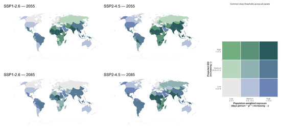
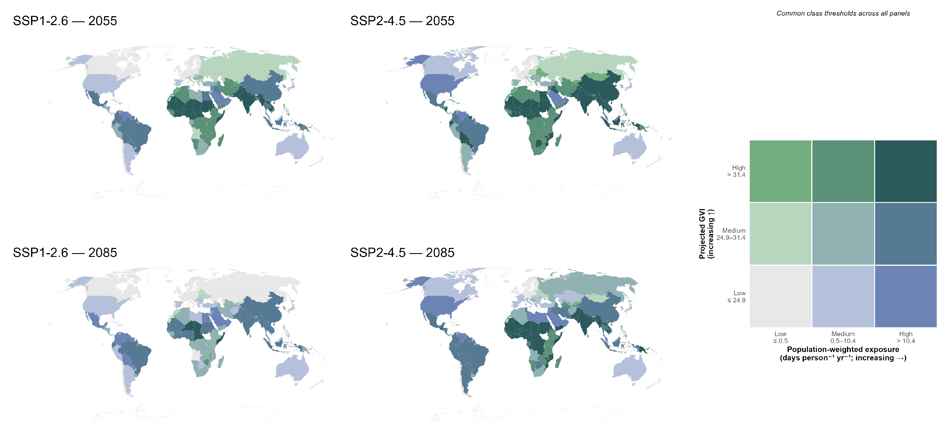
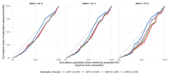
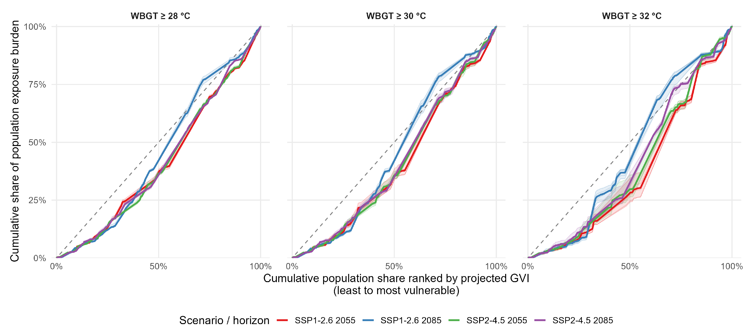
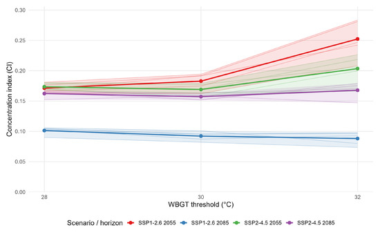
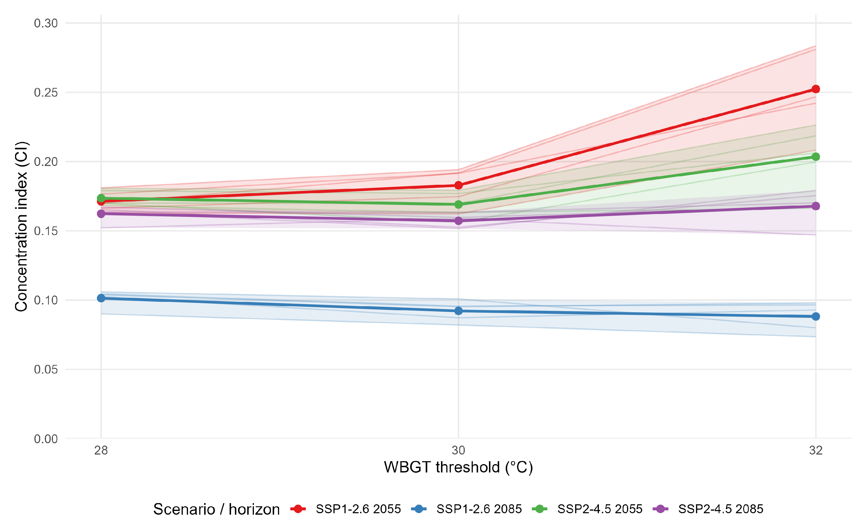
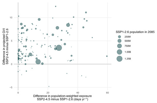
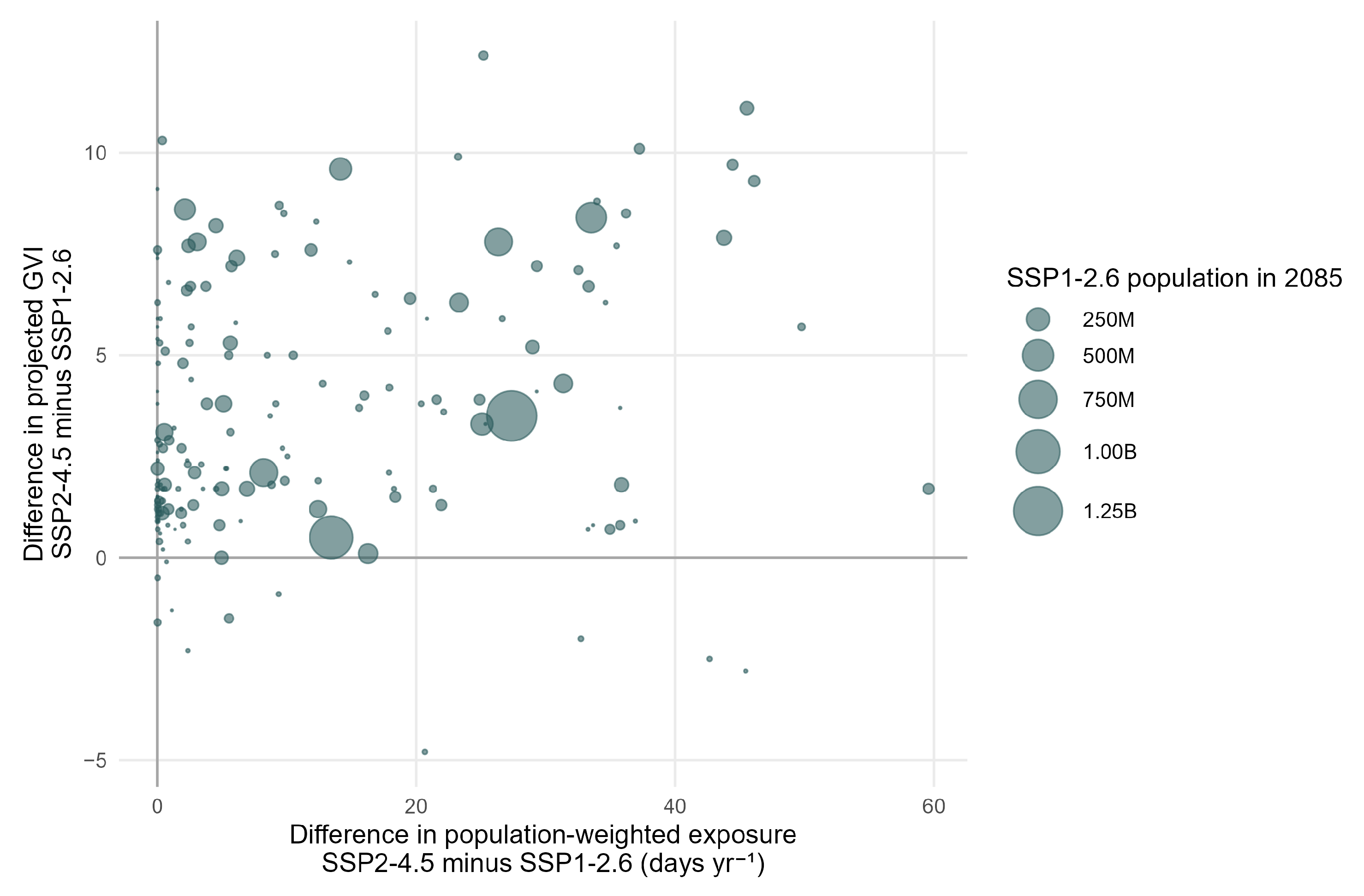
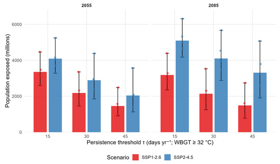
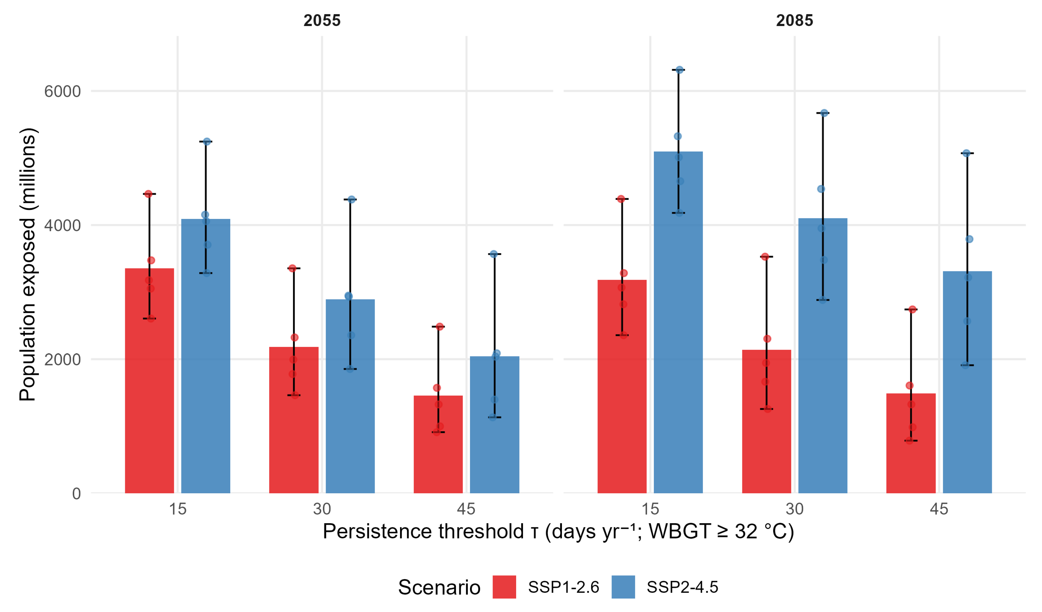

Disclaimer/Publisher’s Note: The statements, opinions and data contained in all publications are solely those of the individual author(s) and contributor(s) and not of MDPI and/or the editor(s). MDPI and/or the editor(s) disclaim responsibility for any injury to people or property resulting from any ideas, methods, instructions or products referred to in the content. |
© 2026 by the author. Licensee MDPI, Basel, Switzerland. This article is an open access article distributed under the terms and conditions of the Creative Commons Attribution (CC BY) license.