A Risk-Informed Digital Twin Framework for Sustainable Construction Scheduling and Carbon Optimization Under Uncertainty

Abstract

The construction sector accounts for 34% of global energy-related CO₂ emissions, yet existing Digital Twin (DT) applications in construction remain largely descriptive, lacking the predictive and prescriptive capabilities required for proactive execution management. This study presents and evaluates, as a simulation-based proof of concept, a risk-informed DT framework integrating a formalized DT state transition model, a dual deep learning prediction engine (Long Short-Term Memory (LSTM) and Transformer), Monte Carlo-based probabilistic carbon quantification for lifecycle modules A1–A5 (S = 10,000), and a risk-adjusted, Non-dominated Sorting Genetic Algorithm II (NSGA-II) optimizer incorporating carbon variance, within a closed weekly feedback loop. The framework is evaluated across five European case studies (residential, education, and commercial office; the Netherlands, the UK, and France) anchored to published project data, with primary calibration on a hybrid real–synthetic mid-rise residential building (CS1; 7200 m², eight stories, the Netherlands) and a fully documented synthetic layer generating the execution records that the published sources do not provide. Under common random number simulation with 50 execution realizations per case, the full framework achieved simultaneous improvements of 5.8–13.2% in expected schedule duration and 10.4–16.4% in expected embodied carbon relative to a static Critical Path Method (CPM) baseline; for CS1, mean intensity fell from 476 to 426 kgCO₂e/m². Component ablation identified the bi-objective optimizer as the dominant contributor, producing an 11.7–20.2% carbon increase when removed, and the selected Pareto solution was invariant to the risk-aversion parameter λ over [0, 1], indicating that risk adjustment functions as a conservatism margin on the reported carbon target rather than a decision-altering preference. The framework advances construction DTs from descriptive monitoring tools toward risk-informed decision support, offering a transparent and reproducible benchmark that advances data-driven sustainability in construction scheduling and embodied carbon management.

1. Introduction

The construction sector accounts for approximately 34% of global energy-related CO₂ emissions and 32% of final energy demand [1], yet it remains one of the least digitally transformed industries. Construction projects routinely experience cost overruns and schedule delays [2], with large-project cost overruns averaging 79% and schedule slippage averaging 52% [3], and 70% of infrastructure projects experiencing delays with an average overrun of 73% [4]. These inefficiencies are compounded by deep-rooted productivity stagnation: construction labor productivity has grown at less than 1% per year over the past two decades, compared with 2.8% for the broader global economy [5]. These persistent failures share a common structural cause: project execution relies on static planning tools that cannot adapt to the dynamic and uncertain conditions of real construction sites, creating a fundamental disconnect between project events and management decisions.

Digital Twin (DT) technology offers a pathway beyond static planning by enabling continuous, bidirectional synchronization between physical construction processes and their virtual representations [6]. However, existing DT implementations in construction remain predominantly descriptive because they capture and display project states but lack the predictive and prescriptive layers necessary for proactive execution management [7]. Meanwhile, advances in deep learning forecasting, multi-objective optimization, and probabilistic carbon modeling have each demonstrated independent promise, yet these capabilities have not been integrated into a unified system capable of simultaneously managing schedule performance and carbon emissions under uncertainty.

This paper develops a risk-informed closed-loop DT framework that addresses this gap directly. The framework integrates four core components: a formally defined DT state transition equation, a dual-model AI prediction engine, a five-component probabilistic carbon model, and a risk-adjusted NSGA-II optimizer within a continuously operating feedback loop governed by BIM and IoT observations. The system is primarily evaluated on CS1 (hybrid real–synthetic) with cross-case evaluation on four additional projects drawing on real published project schedule and embodied carbon datasets and benchmarked against three controlled baselines to isolate the contribution of each component.

The novelty of this work lies not in the individual components—DTs, LSTM networks, Transformer architectures, Monte Carlo analysis, and NSGA-II are established methods— but in their systematic integration into a unified, risk-informed, and fully documented decision loop for construction scheduling and embodied carbon management, together with a transparent simulation benchmark on which the integrated framework is evaluated against ablated and classical alternatives.

2. Literature Review

Five research streams underpin this framework: DT technology, BIM-based project management, AI-driven forecasting, multi-objective optimization, and probabilistic carbon modeling. The subsections below analyze each stream to identify the gap addressed by this work.

2.1. Digital Twin Technology in Construction

DT research in construction has progressed from conceptual frameworks toward data-integrated monitoring systems, yet the gap between monitoring and adaptive management remains largely unaddressed [8]. Tao et al. [6] formalized the five-dimensional DT model, establishing real-time bidirectional synchronization as its defining characteristic. Pan and Zhang [9] introduced a closed-loop DT for construction integrating BIM, IoT sensors, and process mining; however, the framework relies on near-term extrapolation and incorporates neither probabilistic carbon modeling nor multi-objective optimization. Hosamo et al. [7] confirm that existing construction DTs remain descriptive and lack predictive and prescriptive capabilities, the fundamental gap this work addresses.

2.2. Building Information Modeling in Project Management

BIM research has established structured digital representations of construction projects but has not yet extended to simulation-supported adaptive execution management. Sacks et al. [10] demonstrated the value of 4D BIM for schedule planning, while Eastman et al. [11] established BIM as a unified digital representation based on the Industry Foundation Classes (IFC) standard. Despite these advances, BIM-based planning remains static; models are updated episodically with no mechanism for continuous or simulation-driven data ingestion, predictive analytics, or adaptive re-optimization, a gap addressed in this work through the DT integration layer.

2.3. AI-Based Forecasting in Construction

AI forecasting research in construction has progressed from shallow classifiers toward deep sequential architectures, establishing benchmarks against which the dual-model engine developed here is calibrated. Gondia et al. [12] showed that decision tree and naïve Bayes classifiers capture delay risk patterns with accuracy between 74.5% and 78.4%, but without exploiting temporal structure. Laura-Portugal and Hammad [13] demonstrated that LSTM outperforms conventional earned value methods for duration forecasting, while Oliveira and Oliveira [14] showed that Transformer architectures excel at long-horizon energy prediction. Shi and Shide [15] provided the most comprehensive construction benchmark, reporting R² values of 0.94, 0.91, and 0.88 for Transformer, LSTM, and GRU, respectively, which directly informed the task-specific model assignment in this work.

2.4. Multi-Objective Optimization in Construction

Multi-objective optimization research in construction has addressed time–cost–quality trade-offs effectively but has not incorporated carbon emissions or uncertainty within a DT feedback framework. NSGA-II [16] is widely adopted due to its non-dominated sorting and crowding distance mechanisms. Soni et al. [17] applied a hybrid AHP-NSGA-II model to time–cost–quality optimization, demonstrating Pareto-optimal capability; however, neither carbon nor probabilistic uncertainty was included, and no DT feedback mechanism was employed. This work extends the formulation by introducing carbon variance as an explicit penalty term embedded within a simulation-based DT framework.

2.5. Probabilistic Carbon Modeling in Construction

Probabilistic carbon modeling has demonstrated the inadequacy of deterministic LCA approaches but has remained disconnected from real-time scheduling and optimization systems. Huang and Wang [18] applied Monte Carlo quantification to the building materialization phase, showing that probabilistic treatment produces 95% confidence intervals exceeding deterministic estimates by 8.85%, indicating systematic underestimation. Hammond and Jones [19] compiled the ICE database, establishing the material-level emission factor as the standard unit of construction LCA. Both frameworks, however, operate post hoc and are disconnected from any scheduling or optimization system. The SODA framework of Amro and Naimi [20], validated on 50 Dutch buildings, serves as a complementary design-phase reference for the execution-phase system developed here. Table 1 provides a consolidated summary of the key studies reviewed.

Table 1. Summary of Prior Studies Reviewed.

Author(s)	Focus	Method	Limitation/Gap
Tao et al. [6]	Five-dimensional DT model	Conceptual DT framework	No construction application; no scheduling or carbon integration
Lu et al. [8]	DT in smart manufacturing	Systematic review + DT model	Manufacturing-focused; inapplicable to construction execution
Pan & Zhang [9]	BIM-IoT closed-loop DT for construction	Process mining + time series	No deep learning; no probabilistic carbon; no multi-objective optimization
Sacks et al. [10]	4D BIM for scheduling	BIM 4D/5D	Static planning; no real-time AI or adaptive feedback
Eastman et al. [11]	BIM Handbook IFC standard	BIM/IFC	Design-phase focus; no execution-phase DT or carbon
Gondia et al. [12]	ML for construction delay prediction	Decision Tree, Naive Bayes, SVM	No LSTM/Transformer; no carbon objective; no DT feedback
Laura-Portugal & Hammad [13]	LSTM for duration-at-completion	LSTM, MLP, CONV-1D	Schedule only; no carbon integration; no DT loop
Oliveira & Oliveira [14]	Transformer for building energy forecasting	Multi-head Transformer	Operational energy only; not construction execution
Shi & Shide [15]	LSTM vs GRU vs Transformer for cost	LSTM, GRU, Transformer	Cost prediction only; no scheduling, carbon, or DT
Deb et al. [16]	NSGA-II multi-objective algorithm	Non-dominated sorting + crowding	General algorithm; not applied to DT or A1–A5 carbon
Soni et al. [17]	AHP-NSGA-II for time–cost–quality	AHP + NSGA-II	No carbon objective; no uncertainty; no DT feedback
Huang & Wang [18]	Monte Carlo for materialization carbon	Monte Carlo + DQI hybrid	LCA phase only; no AI prediction or real-time optimization
Hammond & Jones [19]	ICE database embodied carbon factors	LCA database	Static emission factors; no uncertainty or DT integration
Amro & Naimi [20]	SODA framework 50 Dutch buildings	Symmetry detection + optimization	Design-phase only; no execution management or DT

Across the five streams reviewed, a consistent gap emerges: DTs lack AI capability [7,9]; AI models are standalone without optimization or DT integration [12,13,14,15]; multi-objective optimization excludes carbon and uncertainty [16,17]; and carbon models are deterministic and disconnected from scheduling [18,19]. No existing work integrates BIM, IoT monitoring, dual-model deep learning, probabilistic five-component carbon modeling, and risk-adjusted optimization within a formally governed DT feedback loop. This convergence constitutes the specific contribution of this study.

3. Materials and Methods

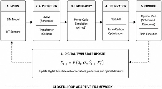
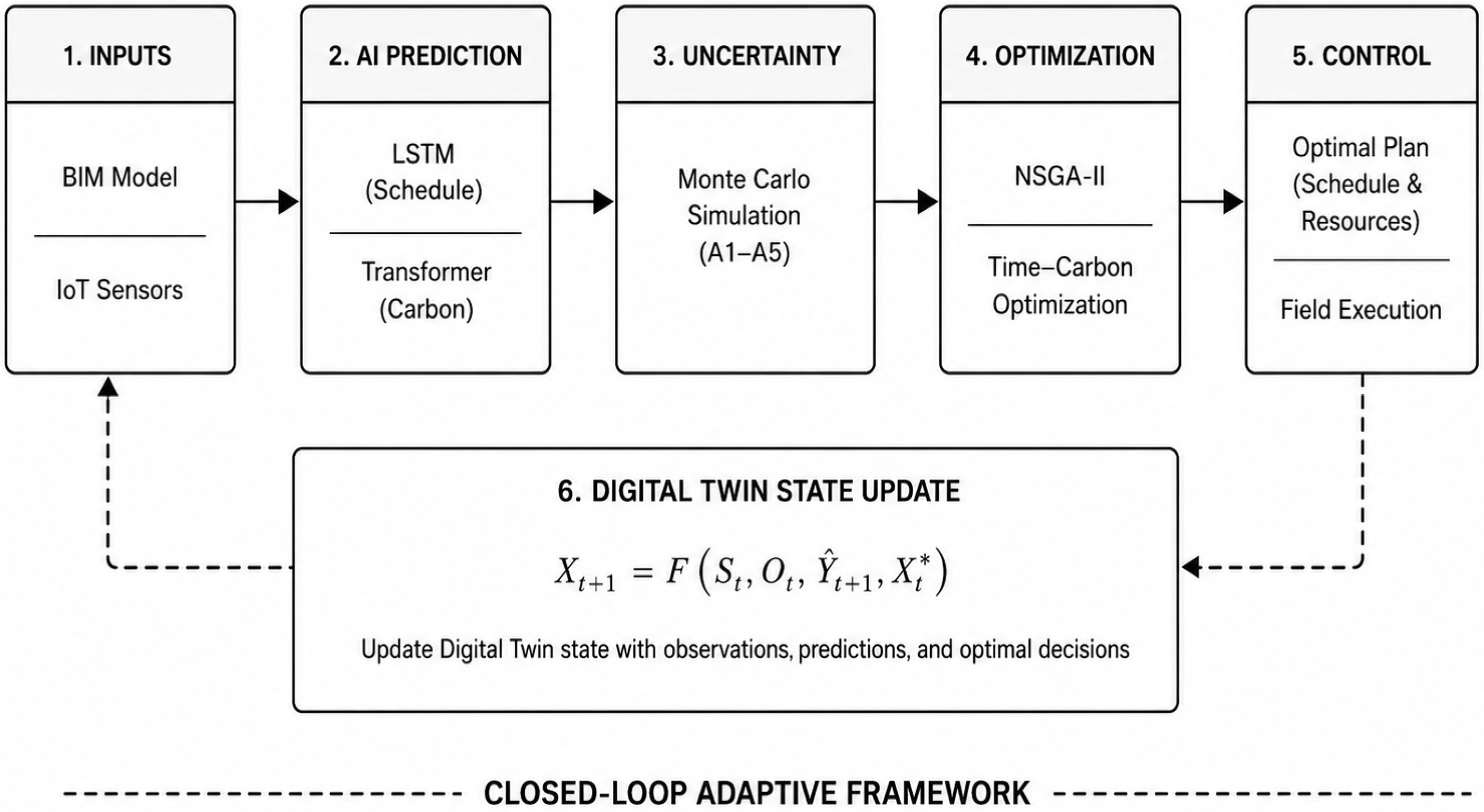
Building on the limitations identified, specifically the absence of closed-loop AI-driven prediction, probabilistic carbon modeling, and risk-aware optimization in existing construction DT implementations, this section presents the developed framework in six stages: overall architecture, the DT state transition equation, the AI prediction engine, the probabilistic carbon model, the NSGA-II optimization formulation, and the case study descriptions. Figure 1 illustrates the closed-loop architecture.

Figure 1. Overview of the closed-loop DT framework developed in this study.

3.1. Framework Architecture

The framework operates as a six-step closed-loop DT. At each discrete time step t, field data collected by IoT sensors and the BIM model are fed into the AI prediction engine, whose outputs drive the NSGA-II optimizer. The resulting optimal decision is applied to update the DT state, which then re-triggers the cycle at $t+1$. Table 2 summarizes the five modules, their methods, functions, and outputs.

Table 2. Framework Modules, Methods, Functions, and Outputs.

Module	Method/Tool	Function	Output
BIM Integration	IFC (Industry Foundation Classes) standard	Extract activity sequences, material quantities, and resource assignments	4D BIM model schedule and material data
IoT Observation	Sensor network/IoT sensors	Record field deviations in progress, energy, materials, and equipment	Observation vector ${\mathrm{O}}_t$
AI Prediction	LSTM + Transformer	Forecast schedule delay risk and remaining carbon emission	Prediction vector ${\widehat{\mathrm{Y}}}_{t+1}$
NSGA-II Optimization	NSGA-II; pop = 48, gen = 50	Generate Pareto-optimal decisions minimizing schedule and risk-adjusted carbon	Optimal decision vector ${\mathrm{X}}_t^{*}$
DT State Update	State transition equation (Equation 1)	Synchronize virtual model with physical site and re-trigger the loop	Updated state ${\mathrm{S}}_{t+1}$

Notes: $O_t$ = IoT observation vector (progress, energy, material, and equipment deviations); $Y_{t+1}$ = AI prediction vector comprising ${\widehat{T}}_{\mathrm{r}\mathrm{e}\mathrm{m}}$, ${\widehat{C}}_{\mathrm{r}\mathrm{e}\mathrm{m}}$, and ${\widehat{D}}_{\mathrm{r}\mathrm{i}\mathrm{s}\mathrm{k}}$; $X_t^{*}$ = Pareto-optimal decision vector obtained from NSGA-II; $S_{t+1}$ = updated digital twin state vector at time step $t+1$.

Model Assumptions

The following assumptions underline the framework. First, construction activity durations and field deviations are assumed to follow stationary stochastic processes within each project phase, such that logged distributions calibrated to historical data remain valid over the 52-week program. Second, the relationship between IoT observations and project state is assumed to be observable with bounded measurement error, consistent with typical sensor accuracy specifications for construction grade IoT systems, while realistic telemetry artifacts (dropouts, drift, systematic bias) are not modeled and represent a core limitation of the current framework. Third, LSTM and Transformer predictions are treated as conditionally independent given the shared input sequence, which simplifies the joint optimization problem without material loss of generality. Fourth, emission factors are assumed to be time invariant over the construction period, which is standard practice in construction LCA consistent with EN 15978 [21]. Fifth, NSGA-II convergence was verified rather than assumed: the two objective hypervolume indicator was tracked across generations for each case, using a population of 48 over 50 generations, and the hypervolume change over the final ten generations was below 2% (0.3–1.9% across the five cases). Tracking the hypervolume indicator across generations to confirm convergence is consistent with established practice in multi-objective construction optimization studies employing NSGA-II [22].

3.2. Digital Twin State Transition Equation

In plain terms, the DT state transition describes how the virtual model of the project is updated each week based on three sources of information: (1) what the IoT sensors observed on site (O_t); (2) what the AI models predict about the remaining schedule and carbon (${\widehat{\mathrm{Y}}}_{\mathrm{t}+\mathrm{1}}$); and (3) what decision the optimizer has selected (${\mathrm{X}}_{\mathrm{t}}^{*}$). The output is the updated virtual state of the project (S_{t + 1}), which is then used as the basis for the next cycle of predictions and decisions.

Formally, the DT is defined as a time-indexed state machine. At each discrete time step t, the state is updated by Equation (1), consistent with the five-dimensional DT model of Tao et al. [6]. The mapping F is deterministic in structure, but its inputs include stochastic predictions produced by the AI models and stochastic observations $O_t$ from IoT sensors, making the overall system behavior probabilistic:

$$S_{\mathrm{t}+1}= F\left(S_{\mathrm{t}}, O_{\mathrm{t}}, {\hat{\mathrm{Y}}}_{\mathrm{t}+1}, X\ast \mathrm{t}\right)$$

(1)

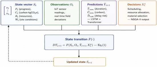
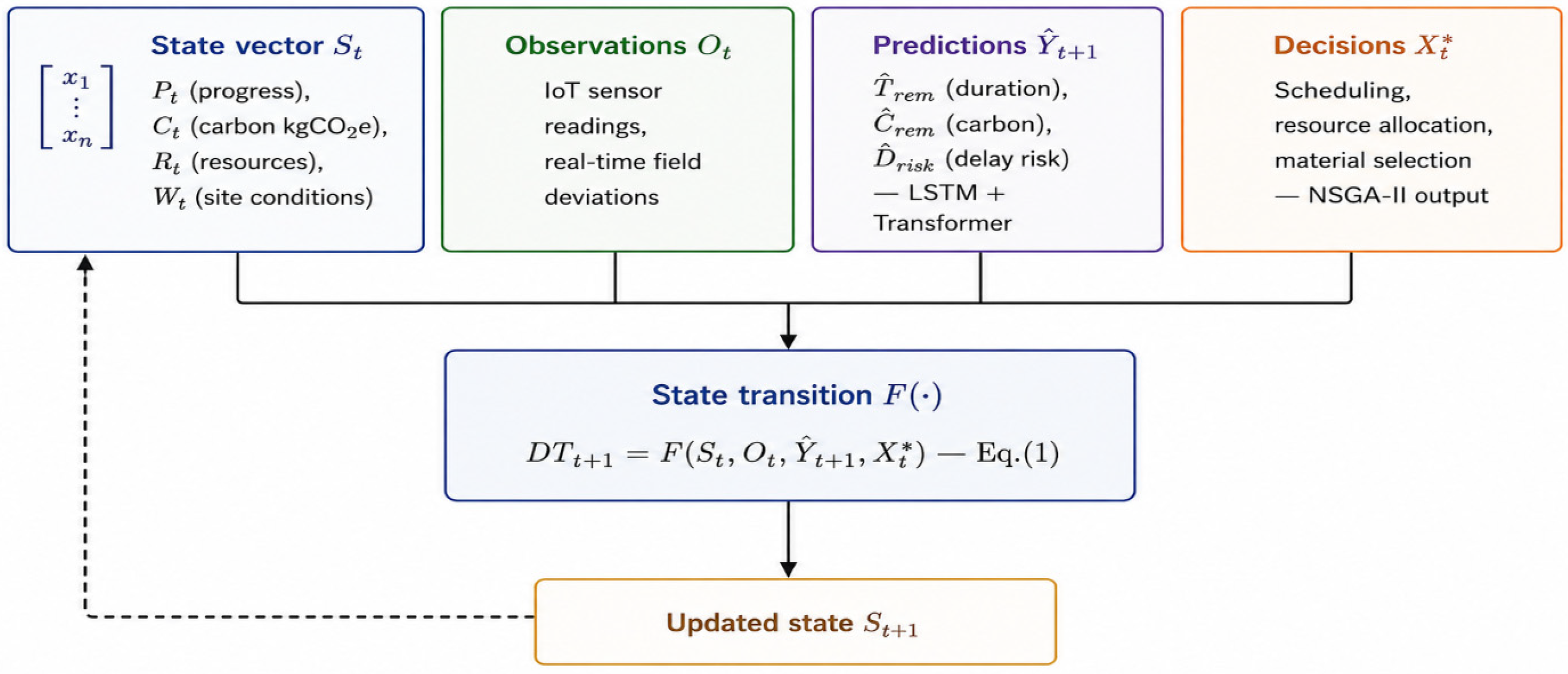
The project state vector $S_t=[P_t,C_t,R_t,W_t,{\mathrm{D}}_{\mathrm{r}\mathrm{i}\mathrm{s}\mathrm{k},\mathrm{t}}]$ captures percentage completion P_t, cumulative carbon C_t (kgCO₂e), available resources R_t, and site conditions W_t and delay-risk state $D_{risk,t}$. The IoT observation vector $O_t={\left[{\delta }_{prog},{\delta }_{energy},{\delta }_{material},{\delta }_{equip}\right]}_t$ represents field deviations. The AI prediction vector ${\widehat{\mathrm{Y}}}_{\mathrm{t}+\mathrm{1}}$ = [${\widehat{\mathrm{T}}}_{\mathrm{r}\mathrm{e}\mathrm{m}}$, ${\widehat{\mathrm{C}}}_{\mathrm{r}\mathrm{e}\mathrm{m}}$, ${\widehat{\mathrm{D}}}_{\mathrm{r}\mathrm{i}\mathrm{s}\mathrm{k}}$] provides the predicted remaining duration, remaining carbon emission, and delay probability. Figure 2 illustrates the five-component structure of the state transition, where the inputs S_t, O_t, ${\widehat{\mathrm{Y}}}_{\mathrm{t}+\mathrm{1}}$, and ${\mathrm{X}}_{\mathrm{t}}^{*}$ are fed into F (·), with the resulting closed-loop feedback from S_{t + 1} back to S_t.

Figure 2. DT state transition at time step t. Inputs S_t, O_t, ${\widehat{\mathrm{Y}}}_{\mathrm{t}+\mathrm{1}}$, and ${\mathrm{X}}_{\mathrm{t}}^{*}$ feed into F (·) [Equation (1)] to produce S_{t + 1}, which feeds back as S_t at the next time step. Adapted from the five-dimensional DT model of Tao et al. [6].

The optimized decision vector ${\mathrm{X}}_{\mathrm{t}}^{*}$ is the output of the NSGA-II module. The state transition follows:

$$St+1=St+\Delta St\left(Ot,Y^t+1,Xt \ast \right)$$

(2)

Equation (2) defines the incremental state update: the new state S_{t + 1} is obtained by applying the optimized decision ${\mathrm{X}}_{\mathrm{t}}^{*}$ and incorporating the latest field observations O_t and the AI predictions ${\widehat{Y}}_{t+1}$into the current state S_t, thereby closing the feedback loop.

The mapping F (·) is operationalized through the following weekly update rules, executed at each checkpoint t, one for each component of the state vector S_t.

(i) Progress (P_t): realized durations of activities started by week t are committed; the remaining network is rescheduled by a CPM forward pass over committed and forecast durations, updating project progress and the projected completion date.

(ii) Cumulative carbon (C_t): material-, transport-, and waste-related carbon accrues in proportion to activity progress, equipment carbon accrues in proportion to realized equipment hours, and site energy carbon accrues linearly with elapsed time (Equations (4)–(8)).

(iii) Available resources (R_t): resource availability reflects the site capacity constraint on concurrent acceleration (x₁ + x₂ ≤ 1.4); the decision vector X_t allocating resources applies only to activities not yet started at week t, while work already started retains the resource and decision levels committed at its start (procurement and shift arrangements are irreversible).

(iv) Site conditions (W_t): site conditions are updated by incorporating realized disruption events (weather, delivery, labor) affecting in-progress activities; their effect persists in the committed durations of affected activities and cannot be reversed at later checkpoints.

(v) Risk state (${\widehat{\mathrm{D}}}_{\mathrm{r}\mathrm{i}\mathrm{s}\mathrm{k}}$): the delay risk indicator is updated from the prediction engine’s forecast of remaining duration relative to the framework’s own initial optimized projection.

Missing or delayed observations are handled by carrying the last available state forward for one checkpoint. Inconsistent BIM information, for example, activity quantities or sequencing that diverge from the as-built network is resolved by treating the BIM-derived activity network, as the authoritative reference at each re-planning cycle; discrepancies detected during a checkpoint are logged but do not retroactively alter committed activities, consistent with the irreversibility rule above.

3.3. Dual-Model AI Prediction Engine

The prediction engine assigns each forecasting task to the architecture best suited to its temporal characteristics. The Long Short-Term Memory (LSTM) network [23] is used to predict ${\widehat{T}}_{\mathrm{rem}}$ and ${\widehat{D}}_{\mathrm{risk}}$ based on short-term sequential patterns in daily and weekly schedule data, as demonstrated by Laura-Portugal and Ayman Hammad [13].

In contrast, the Transformer model [24] is employed to predict ${\widehat{C}}_{\mathrm{rem}}$ through its multi-head self-attention mechanism, which enables the capture of long-range dependencies across the full project timeline more effectively than recurrent architectures for sequences exceeding several hundred time steps [14].

This task-specific assignment is supported empirically by Shi and Shide [15], who benchmarked LSTM, Gated Recurrent Unit (GRU), and Transformer on a construction cost time series, reporting R² values of 0.94, 0.91, and 0.88, respectively, confirming Transformer superiority on long-horizon sequences. For short-horizon schedule prediction, Laura-Portugal and Hammad [13] showed that LSTM outperforms both convolutional and fully connected networks, confirming its suitability for short-term delay forecasting tasks. Both findings directly inform the task assignments adopted in this work.

Both models are trained on the hybrid datasets, combining real project benchmarks with a documented synthetic execution simulator; per case, 60 independently seeded realizations (windows of 12 weeks) provide the training data, with model capacity selected to match this data volume.

3.4. Five-Component Probabilistic Carbon Emission Model

Total pre-use embodied carbon (Modules A1–A5) is decomposed into five components in accordance with the lifecycle stage boundaries defined in EN 15978:2011 [21]:

$$C_{\mathrm{total}}\left(t\right)=C_{\mathrm{mat}}+C_{\mathrm{trans}}+C_{\mathrm{equip}}+C_{\mathrm{waste}}+C_{\mathrm{site}}$$

(3)

The individual components are calculated as follows. Embodied material carbon is computed using Equation (4), transport emissions using Equation (5), equipment fuel emissions using Equation (6), waste disposal emissions using Equation (7), and site energy emissions using Equation (8):

$$C_{\mathrm{mat}}=\sum _i\left(Q_i\times E{F}_i\right)$$

(4)

where $Q_i$ represents the quantity of material $i$ (kg), and $E{F}_i$ denotes the corresponding emission factor (kgCO₂e/kg), sourced from ecoinvent v3 (Ecoinvent Center, Zurich, Switzerland) and ICE v3.

$$C_{\mathrm{trans}}=\sum _i\left(Q_i\times d_i\times 0.062\right)$$

(5)

where $d_i$ is the transport distance (km), and 0.062 represents the emission factor (kgCO₂e/tonne·km), consistent with EN 16258:2012 and Department for Energy Security and Net Zero (DESNZ, 2024) [25].

$$C_{\mathrm{equip}}=\sum _j\left(P_j\times t_j\times 2.68\right)$$

(6)

where $P_j$ is the equipment fuel consumption rate (liter/hour), $t_j$ is the operating time (hours), and 2.68 is the diesel emission factor (kgCO₂e/liter), based on Intergovernmental Panel on Climate Change (IPCC, 2006) [26].

$$C_{\mathrm{waste}}=\sum _i\left(W_i\times E{F}_{\mathrm{disposal},i}\right)$$

(7)

where $W_i$ represents waste quantity (kg) and $E{F}_{\mathrm{disposal},i}$ is the disposal emission factor obtained from ecoinvent v3.

$$C_{\mathrm{site}}=E_{\mathrm{site}}\times E{F}_{\mathrm{grid}}$$

(8)

where $E_{\mathrm{site}}$ denotes site energy consumption (kWh), and $E{F}_{\mathrm{grid}}$ is the grid emission factor (kgCO₂e/kWh), based on DESNZ (2024) [25].

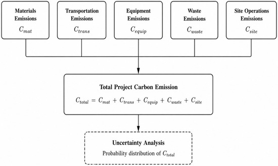
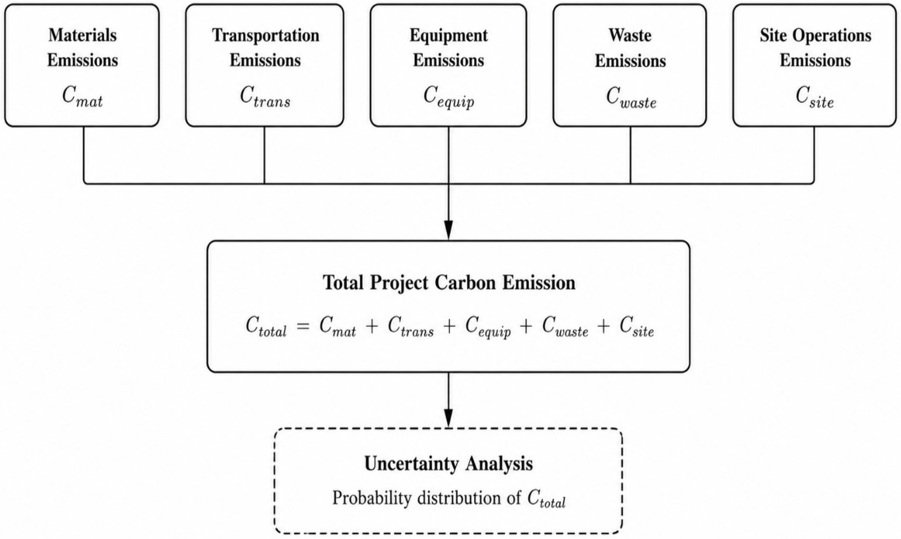
Figure 3 illustrates the structure of the five-component carbon emission model, along with the Monte Carlo uncertainty layer applied to $C_{total}$.

Figure 3. Five-component carbon emission model aggregating into $C_{total}$, with Monte Carlo uncertainty quantification (S = 10,000 simulations).

To account for parameter uncertainty, a Monte Carlo layer with S = 10,000 draws is implemented (Equation (9)). Emission factors are modeled as truncated normal distributions (truncation at 0.2 of the mean, preventing non-physical negative factors) with a coefficient of variation of 0.10, consistent with the pedigree-based data quality ranges reported for the ecoinvent database [27]; the coefficient of variation is widened in proportion to the material-substitution level (×(1 + 0.8· $x_{sub}$)), reflecting the less mature supply chains and wider declared ranges of novel low-carbon materials. Transport distances follow uniform distributions U (0.8d, 1.2d) around the case supply distances, and activity durations follow lognormal distributions with coefficients of variation of 0.10, 0.20, and 0.30 for low-, medium-, and high-variability activity classes, following the schedule uncertainty evidence of Ballesteros-Pérez et al. [28]; the lognormal family reproduces the non-negativity and right skewness observed in realized construction durations. Correlation across the schedule and carbon domains is induced structurally rather than assumed: realized durations enter the equipment energy and site energy terms directly so that schedule outcomes and process carbon are physically coupled (the simulated correlation between realized duration and realized carbon is 0.94).

Correlations among the five carbon components themselves are also structural rather than independently assumed: material, waste, and transport carbon all scale with the same underlying material quantities ($Q_i$ in Equations (4), (5), and (7)), so an increase in material use raises all three jointly; equipment carbon scales with realized activity duration (Equation (6)), directly linking it to the schedule dynamics above; only site energy carbon (Equation (8)) is independent of material quantities, depending instead on elapsed project time.

Emission factor and transport distance distributions follow ecoinvent’s pedigree-based data quality framework [27] and standard construction logistics practice, respectively; the lognormal duration distribution follows the construction-specific schedule uncertainty evidence of Ballesteros-Pérez et al. [28]. Table 3 verifies that the results are not sensitive to the specific parametric family assumed: each distribution was individually replaced with an alternative of matched mean and variance, and all resulting differences in carbon and schedule statistics remained below 0.01%.

Table 3. Distributional Sensitivity Check—CS1 Selected Solution (S = 10,000).

Alternative Distribution Tested	$\mathit{\mu }\mathit{C}$ diff (%)	$\mathit{\sigma }\mathit{C}$ diff (%)	$\mathit{E}\left[\mathit{T}\right]$ diff (%)
Emission factors: truncated normal → uniform (matched variance)	+0.0001	+0.0800	—
Transport distance: uniform → normal (matched variance)	+0.0001	+0.0008	+0.0000
Activity duration: lognormal → normal (matched variance)	+0.0008	−0.0021	+0.0082

Notes: All alternatives share the same mean and variance as the distribution used in the paper, isolating the effect of distributional shape. Baseline (as used in paper): $\mu C$ = 2894.15 t, $\sigma C$= 271.47 t, E[T] = 46.64 wk.

A deterministic carbon model yields a single point estimate, which conceals the uncertainty arising from variable emission factors, transport distances, and activity durations. To quantify this uncertainty explicitly, the model outputs a full probability distribution rather than a single value, enabling the optimizer to penalize not only the expected carbon but also its variance. The resulting distribution is:

$$C_{\mathrm{total}}\left(t\right)\sim \mathrm{Empirical}({\mu }_C,{\sigma }_C,P_5,P_{95})$$

(9)

Equation (9) defines the Monte Carlo estimator. For each simulation run $s$, total carbon emissions are computed as the sum of the five model components. The statistical descriptors ${\mu }_C$, ${\sigma }_C$, $P_5$, and $P_{95}$ are then derived empirically from the resulting sample of $S=\mathrm{10,000}$ realizations, without assuming any predefined parametric distribution.

These statistical outputs are subsequently passed to the NSGA-II optimizer in Equation (10). The Monte Carlo procedure follows the five-component structure defined in Equations (4)–(8).

Throughout the paper, absolute emissions are reported in tCO₂e and area-normalized intensities in kgCO₂e/m²; intensities equal absolute values divided by the gross floor area.

3.5. Risk-Adjusted NSGA-II Optimization

NSGA-II [16] is selected over more recent variants, including NSGA-III and MOEA/D, for three reasons. First, the bi-objective formulation (schedule and carbon) is well within the two- to three-objective range for which NSGA-II consistently demonstrates strong Pareto front quality [16,17]. Second, NSGA-II has an established track record in construction scheduling optimization [17], providing direct comparability with prior work. Third, its crowding distance mechanism offers well-understood diversity preservation without requiring reference point tuning, which is appropriate given the absence of domain-specific reference data for combined carbon schedule optimization. Future work should examine whether NSGA-III or many objective variants provide additional benefit when the objective space is extended.

The Non-dominated Sorting Genetic Algorithm II (NSGA-II) [16] is employed to simultaneously minimize two objectives: the expected remaining project duration and a risk-penalized carbon target:

$$\min \left[\mathbb{E}\left({\widehat{T}}_{\mathrm{rem}}\right), \mathbb{E}\left({\widehat{C}}_{\mathrm{rem}}\right)+\lambda \cdot {\sigma }_{{\widehat{C}}_{\mathrm{rem}}}\right]$$

(10)

subject to the resource constraint x₁ + x₂ ≤ 1.4 (structural and fit-out acceleration cannot both run at full intensity simultaneously), enforced by a penalty added to both objectives upon violation; activity precedence is satisfied by construction, since decisions modify activity durations within a CPM forward pass. The carbon budget $C_{limit}$ is not imposed as a hard optimization constraint but is evaluated post hoc as a compliance probability $P\left(C_{total}\le C_{limit}\right)$.

Each candidate solution is encoded as a real-valued chromosome x ∈ [0, 1]⁶: structural works acceleration (x₁, up to −18% duration at the cost of +45% equipment fuel), fit-out acceleration (x₂, up to −15% duration, +35% fuel), low-carbon material substitution (x₃, reducing effective material emission factors up to a frame-specific ceiling while slowing the cast-in-place structural cycle by up to +10% and adding a procurement lead time on foundations), equipment idle reduction scheduling (x₄, up to −35% fuel), site energy management (x₅, up to −25% site electricity), and envelope fast-tracking (x₆). Effect ceilings are conservative literature bounds and cap what optimization can achieve.

This formulation enables reduction of $C_{mat}$ through material substitution (x₃), in addition to reducing $C_{equip}Cequip$ through optimized equipment scheduling (x₁, x₂, x₄). The risk aversion parameter λ controls the penalty applied to carbon variability, where higher values of λ favor solutions with lower carbon uncertainty; The selected solution is shown to be invariant to λ over [0, 1].

Objectives are evaluated on a fixed set of 24 pre-drawn uncertainty scenarios shared by all candidates (common random numbers), removing Monte Carlo noise from candidate comparisons. The algorithm is implemented with a population size of 48 and 50 generations, using simulated binary crossover ($\eta c$ = 15, pc = 0.9) and polynomial mutation ($\eta m$ = 20, pm = 1/6), following Deb et al. [16]. The preferred solution is the Pareto point minimizing the normalized Euclidean distance to the utopia point of the front; this solution is subsequently applied in Equation (2) to update the DT state.

The four system components are integrated into a complete closed-loop weekly execution workflow, summarized in Appendix A (Algorithm A1). In brief, at each discrete time step t: (1) the DT state is updated from IoT observations via Equation (1); (2) LSTM and Transformer models generate schedule and carbon predictions; (3) Monte Carlo sampling quantifies carbon uncertainty via Equations (4)–(9); and (4) NSGA-II solves the bi-objective problem of Equation (10) when a delay risk alert is triggered $\left(D_{risk}> \theta \right)$ or at periodic re-optimization intervals. The resulting Pareto-optimal decision vector $X_t^{*}$ is applied to update the DT state for the next time step.

3.6. Baseline Configurations

The framework is benchmarked against three baselines, each designed to isolate the contribution of a specific component. Table 4 describes the three baselines and the component each one tests.

Table 4. Baseline Configurations and Component Each Tests.

Baseline	Description	Component Tested	Expected Outcome
B1 Static CPM	Fixed critical-path schedule; no monitoring feedback, no AI, no optimization	Value of the entire closed-loop DT framework	Highest delay and carbon; reference baseline
B2 Descriptive DT	DT with IoT monitoring; a fixed manual acceleration is applied once an observed progress gap exceeds a threshold; no AI forecasting, no NSGA-II optimization, no carbon-aware decisions	Value of the AI prediction and optimization layers beyond passive monitoring	Partial schedule recovery through manual response; carbon essentially unchanged
B3 Schedule-only	Single-objective optimization (grid search over acceleration variables only) applied from the outset; no AI feedback loop, no carbon co-objective; other decision variables held at baseline	Value of carbon as a co-objective in the optimization formulation	Fastest schedule; no carbon benefit and, for equipment-intensive cases, a carbon increase

Performance is evaluated across five metrics: schedule improvement (percentage reduction in project duration versus B1), carbon reduction (percentage reduction in expected $C_{\mathrm{total}}$ versus B1), prediction accuracy (RMSE and MAPE for ${\widehat{T}}_{\mathrm{rem}}$ and ${\widehat{C}}_{\mathrm{rem}}$), Pareto front quality (hypervolume indicator HV and inverted generational distance IGD), and carbon uncertainty coverage (width of the 90% confidence interval $P_5$-to-$P_{95}$ from Equation (9)).

To further isolate the contribution of the optimization layer itself, a fifth configuration, a simple, non-optimized heuristic baseline, was evaluated under the same 50-realization common random numbers protocol as B1–B3 and the full system. The heuristic applies fixed, round-number decision levels (0.5 on structural acceleration, fit-out acceleration, material substitution, equipment idle reduction, and site energy management, with no fast-tracking) statically from project start, representing a plausible rule-of-thumb response by an experienced project manager without any optimization algorithm or AI feedback. As shown in Table 5, the heuristic improves modestly on B1 (2.6–5.4% schedule and 7.3–14.4% carbon) but remains clearly inferior to the full framework on schedule (1.8–9.7% slower), confirming that systematic optimization rather than any reasonable fixed policy is required to reach the Pareto-efficient region identified by NSGA-II. This heuristic baseline, together with the λ = 0 configuration that isolates deterministic optimization without a variance penalty, further decomposes the B1–B3 comparison and establishes that the reported improvements are not artifacts of an insufficiently competitive baseline set.

Table 5. Simple Heuristic Baseline vs. B1 and the Full System (CS1–CS5).

Case	Heuristic T (wk)	Heuristic C (t)	Δ vs. B1 (T/C)	Δ vs. Full (T/C)
CS1	53.3	2933	+3.4%/+14.3%	+9.4%/−4.4%
CS2	86.3	900	+4.1%/+7.3%	+1.8%/+9.1%
CS3	130.1	2496	+5.4%/+10.0%	+5.9%/+7.7%
CS4	130.4	3298	+4.7%/+10.8%	+9.7%/+1.3%
CS5	111.5	6718	+2.6%/+14.4%	+8.6%/−0.0%

Notes: Positive Δ = improvement. The heuristic applies x = [0.5, 0.5, 0.5, 0.5, 0.5, 0.0] statically, with no forecast-triggered adaptation. Evaluated on the same 50 realizations and common random numbers used throughout this analysis.

This carbon parity arises because the heuristic’s slower, less aggressive schedule reduces acceleration-related equipment fuel, illustrating that the full framework’s advantage lies in reaching a superior schedule carbon trade-off, not merely in minimizing either objective in isolation.

3.7. Case Study Descriptions

3.7.1. Case Study 1: Mid-Rise Residential Building, Netherlands (CS1)

CS1 is an eight-story reinforced concrete (RC) residential building located in the Netherlands (52.37° N, 4.90° E), with a gross floor area (GFA) of 7200 m² and a 52-week construction program comprising 96 activities. The structural system consists of an RC frame with hollow core slabs. The baseline A1–A5 embodied carbon is 469 kgCO₂e/m². CS1 serves as the primary calibration case for the framework. Schedule data are sourced from Thiele et al. [29]; building specifications from Usmanov [30] and Benke et al. [31]; emission factors from ecoinvent v3 [27], ICE v3 [32], and EN 16258:2012 [33].

3.7.2. Case Study 2: The Enterprise Center, Norwich, UK (CS2)

CS2 is a two-story timber education building (University of East Anglia, Norwich, UK; 52.62° N, 1.24° E), with a GFA of 3400 m² and an approximately 85-week program. The structural system is a Brett Stapel and glulam hybrid frame. The normalized A1–A5 embodied carbon is approximately 283 kgCO₂e/m² (±10%), derived from a published 100-year whole-life LCA of 456 kgCO₂e/m². CS2 represents the lowest carbon typology in the dataset. Source: UKGBC [34]; Architype/Morgan Sindall.

3.7.3. Case Study 3: 6 Orsman Road, London, UK (CS3)

CS3 is a six-story hybrid CLT and cellular steel commercial office building in Hackney, London, UK (51.54° N, 0.07° W), with a GFA of 4678 m² and an approximately 130-week program. The structural system combines cross-laminated timber (CLT) floor plates with cellular steel beams on a 7.5 m grid. Whole-building A1–A5 embodied carbon is 582 kgCO₂e/m² (RICS WLCA); structure-only is 238 kgCO₂e/m² (LETI Band A). CS3 represents the highest carbon whole-building reference in the dataset. Source: Waugh Thistleton Architects [35]; LETI [36].

3.7.4. Case Study 4: Hyperion Tower, Bordeaux, France (CS4)

CS4 is a 17-story hybrid RC-CLT residential tower in Bordeaux, France (44.83° N, 0.56° W), with a GFA of 7000 m² and an approximately 130-week program. The structural system comprises an RC core with prefabricated CLT infill wall panels. The normalized A1–A5 embodied carbon is approximately 522 kgCO₂e/m² (±10%), derived from a full-scope published value of 870 kgCO₂e/m² (A1–C4, BBCA Eges). The building holds BBCA certification and an E3C2 energy label. Source: Eiffage Construction [37].

3.7.5. Case Study 5: Three Chamberlain Square, Birmingham, UK (CS5)

CS5 is a ten-story post-tensioned RC commercial office building in Birmingham, UK (52.48° N, 1.90° W), with a GFA of 17,500 m² and an approximately 108-week program. The structural system is a post-tensioned flat slab RC frame, representing a high-carbon conventional construction typology. Published A1–A5 embodied carbon is 449 kgCO₂e/m² (LETI Band B; RICS WLCA), representing the highest carbon reference in the dataset. Source: Cundall [38].

3.7.6. Cross-Case Normalization and Comparative Summary

All baseline embodied carbon values were normalized to the A1–A5 scope prior to framework application. Table 6 presents the normalized comparison across the five case studies, spanning a 299 kgCO₂e/m² optimization range from CS2 (low-carbon timber) to CS3 (whole-building hybrid).

Table 6. Cross-Case Normalized Embodied Carbon and Construction Program Parameters.

Case	Type	Location	GFA (m2)	Floors	Duration (wk)	A1–A5 (kgCO2e/m2)	Structure	Source
CS1	Residential	The Netherlands	7200	8	52	469	RC frame	Benke [31]; Thiele [29]
CS2	Education	Norwich, UK	3400	2	~85	~283 (norm.)	Timber hybrid	UKGBC; Röck [39]
CS3	Office	London, UK	4678	6	~130	582	CLT + steel	Waugh Thistleton; LETI [36]
CS4	Residential	Bordeaux, FR	7000	17	~130	~522 (norm.)	RC core + CLT	Eiffage; Röck [39]
CS5	Office	Birmingham, UK	17,500	10	~108	449	PT-RC frame	Cundall; RICS WLCA

Published carbon figures for the five cases differ in lifecycle boundary and scope. Table 7 records, for each case, the value as published, its original boundary, and the treatment applied to obtain a common A1–A5 basis. Where the source reports A1–A5 directly, the value is adopted unchanged. Where the source reports a wider boundary, the A1–A5 share is estimated from the source’s own module breakdown where available, with the residual conversion uncertainty represented as ±10% in the Monte Carlo layer.

Table 7. Carbon boundary treatment per case.

Case	Published Value	Original Boundary	Treatment to A1–A5	Excluded Items
CS1	469 kgCO2e/m2	A1–A5 directly (Benke dataset [31])	Adopted directly	None (already A1–A5)
CS2	283 kgCO2e/m2 (±10%)	100-year whole-life LCA, 456 kgCO2e/m2 [34]	Normalized to A1–A5 share; ±10% uncertainty applied	Use-stage impacts (B1–B7, including operational energy and component replacement) and end-of-life impacts (C1–C4)
CS3	582 kgCO2e/m2	Whole-building A1–A5 (RICS WLCA) [35]	Adopted directly; structure-only figure (238 kgCO2e/m2, LETI Band A) not used	None (already A1–A5); structure-only alternative figure excluded from use
CS4	522 kgCO2e/m2 (±10%)	Full-scope A1–C4, 870 kgCO2e/m2 (BBCA Eges) [37]	A1–A5 share per source module breakdown; ±10% uncertainty applied	End-of-life impacts (C1–C4: deconstruction, transport, waste processing, disposal)
CS5	449 kgCO2e/m2	A1–A5 directly (LETI Band B; RICS WLCA) [38]	Adopted directly	None (already A1–A5)

3.8. Synthetic Data Generation, Calibration, and Leakage Control

The five case studies combine published project data with a documented stochastic simulation layer. For each building, the typology, gross floor area, story count, structural system, program duration, and A1–A5 embodied carbon benchmark are real values taken from the published sources cited in Section 3.7. What no published source provides, and what, therefore, must be simulated, is the weekly execution record: activity-level progress, disruption events, IoT deviation streams, and the counterfactual outcomes of management interventions that were never applied on the real sites. Table 8 demarcates these categories explicitly for each case.

Table 8. Real versus synthetic inputs per case study.

Input	CS1	CS2	CS3	CS4	CS5	Status
Typology, GFA, stories, structural system	Yes	Yes	Yes	Yes	Yes	Real (published)
Program duration (planned)	Yes	Yes	Yes	Yes	Yes	Real (published)
A1–A5 embodied carbon benchmark (kgCO2e/m2)	Yes	Yes	Yes	Yes	Yes	Real (published; conversion documented in Section 3.7.6)
Emission factors (materials, transport, fuel, grid)	Yes	Yes	Yes	Yes	Yes	Real (ecoinvent v3, ICE v3, EN 16258, IPCC)
Activity network (topology, precedence)	No	No	No	No	No	Synthetic (template)
Weekly progress and disruption events	No	No	No	No	No	Synthetic (stochastic model)
IoT deviation streams	No	No	No	No	No	Synthetic (AR (1) model)
Baseline-configuration outcomes (B1–B3, Full)	No	No	No	No	No	Simulated counterfactuals

Generation mechanism. Each case is represented by an activity-on-node network built from a common construction phasing template (substructure, a per-story structural cycle, story-wise envelope and fit-out chains lagged one story behind the structure, and building-wide closeout), yielding 10f + 16 activities for a building of f stories. Precedence follows finish-to-start logic within trade chains, with envelope work gated on the structure above and interior work gated on weather tightness. Template durations are scaled by a case-specific factor, so the deterministic critical path matches the published program exactly. Realized durations, disruption events, and IoT observation noise follow the lognormal, Poisson, and AR (1) specifications summarized in Table 9; observations are therefore informative but imperfect, consistent with construction grade sensing rather than idealized telemetry. Each activity also carries physical quantities (material tonnage, haul distance, equipment fuel, waste fraction) from trade-level intensity profiles, coupling schedule and carbon directly: a delayed realization consumes more site energy and equipment hours.

Table 9. Simulation parameters, values, and sources.

Parameter	Value	Source/Status
Duration distribution	Lognormal, E[X] = plan	[28]
Duration CV (low/med/high class)	0.10/0.20/0.30	[28]
Disruption arrival rate	0.06 wk−1	Assumption, calibrated to delay statistics [3,4]
Disruption severity	U (0.5, 2.0) wk	Assumption
IoT autocorrelation ρ	0.6	Assumption
Supplier EF variation (per realization)	TruncN, CV = 0.08	Assumption (batch variability)
Epistemic EF uncertainty (MC layer)	TruncN, CV = 0.10; widened by substitution level	ecoinvent data quality ranges [27]
Transport distance uncertainty	U (0.8d, 1.2d)	Assumption
Emission factors	ecoinvent v3, ICE v3, EN 16258, IPCC 2006; grid 0.270 kgCO2e/kWh	Published
Lookback window/channels	12 wk/7	Design choice
Split level	Realization (project) level	Design choice (leakage control)
Random seeds	Loop 50,000+r; trajectories 200,000+10,000·i+r; NSGA-II 3/11/17 (search), 7 (scenarios); Torch 0	Reported for reproducibility

Dataset construction and leakage control. Training and evaluation windows are extracted from complete, independently seeded project realizations, with the split performed at the realization level: a simulated project belongs entirely to the training or entirely to the test set, and no test realization window is visible during training or validation.

Calibration. Two scalar calibrations anchor each simulated case to its published record: a time-scale factor matching the deterministic critical path to the published program duration, and a material quantity scale factor matching the deterministic A1–A5 total to the published benchmark. Both are held fixed across all experiments; no result-level quantity is tuned. Table 9 summarizes all simulation parameters, their adopted values, and sources.

4. Results

Results are reported across all five case studies (CS1–CS5). Uncertainty is quantified via 50 independently seeded execution realizations per configuration, evaluated under common random numbers across configurations.

4.1. Experimental Setup

Training and evaluation data were generated by a documented stochastic execution simulator, combining published project benchmarks with synthetic weekly execution records: for each case, 60 independently seeded execution realizations were used for training and 15 disjoint realizations for testing, with windows of 12 weeks over seven feature channels. The split was performed at the realization level, so no augmented window from a test project appears in training; validation for early stopping used 15% of the training windows. The same LSTM and Transformer architecture and input dimensionality (Table 10) were applied to each case, trained independently per case.

Table 10. Model Hyperparameters and Training Configuration.

Hyperparameter	LSTM (${\mathit{T}}_{\mathit{r}\mathit{e}\mathit{m}},{\mathit{D}}_{\mathit{r}\mathit{i}\mathit{s}\mathit{k}}$)	Transformer (${\mathit{C}}_{\mathit{r}\mathit{e}\mathit{m}}$)
$\mathrm{Hidden} \mathrm{units}/d_{model}$	64 units (2 layers)	$d_{model}$ = 64, 4 heads, 1 encoder layer
Lookback window k	12 weeks	12 weeks
Batch size	128	128
Epochs	30 (patience = 5)	30 (patience = 5)
Optimizer	Adam (lr = 0.001)	Adam (lr = 0.0005)
Loss function	$\mathrm{MSE} (T_{rem}$$); \mathrm{BCE} (D_{risk}$)	MSE
Dropout	0.2	0.1
Train/Test realizations per case	60/15 (realization-level split)	60/15 (realization-level split)

Note: NSGA-II used a population of 48, 50 generations, simulated binary crossover ($\eta c$ = 15), polynomial mutation ($\eta m$ = 20), following Deb et al. [16]. Monte Carlo: S = 10,000 draws per case.

Hyperparameters in Table 10 were not formally tuned via grid or random search, due to the single-CPU compute budget available; compact settings were selected directly and held fixed across all cases. To verify that reported results are not fragile to this choice, a sensitivity check (Table 11) compared the settings used against three alternatives (halved hidden size, doubled hidden size, and extended training with a smaller batch) on CS1. Performance remained stable across all four configurations (LSTM R² = 0.953–0.972; Transformer R² = 0.944–0.973), with the settings used in the paper close to the upper end of this range rather than an outlier, indicating that the reported findings are not an artifact of a fortunate hyperparameter choice.

Table 11. Hyperparameter Sensitivity Check on CS1.

Configuration	LSTM R2	LSTM RMSE (wk)	Transformer R2	Transformer RMSE (t)
Used in paper (hidden = 64)	0.965	2.41	0.968	187.0
Smaller (hidden = 32)	0.953	2.81	0.944	245.7
Larger (hidden = 128)	0.972	2.16	0.973	169.3
More epochs, smaller batch	0.972	2.17	0.969	181.5

4.2. AI Prediction Engine Performance

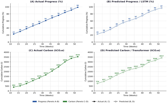
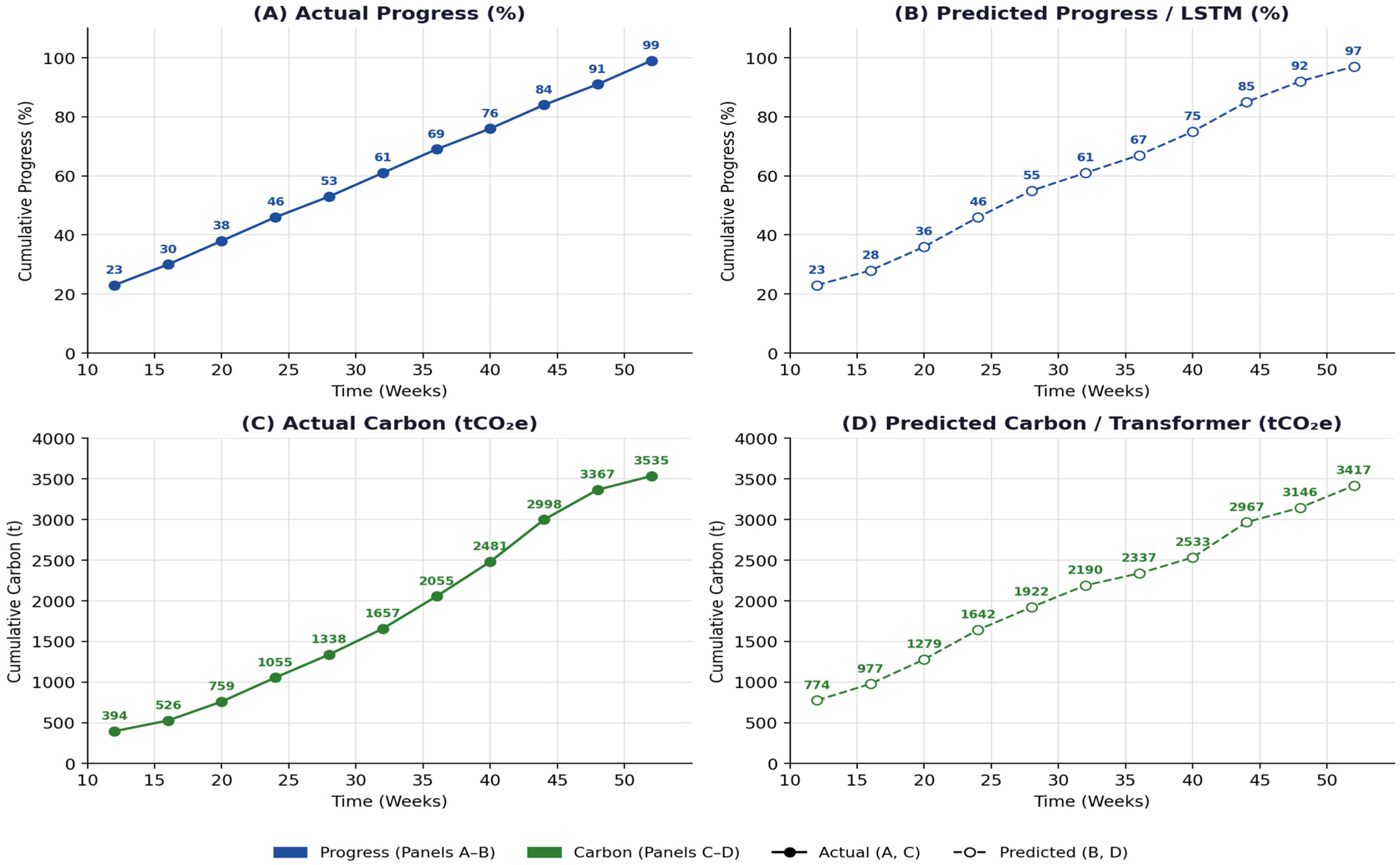
Table 12 reports the dual-model prediction accuracy across all five case studies, evaluated on 15 disjoint held-out execution realizations per case. LSTM RMSE is expressed in weeks; Transformer RMSE in tCO₂e. All R² values exceed 0.96, confirming consistent predictive performance across building typologies. Figure 4 illustrates actual vs. predicted trajectories for CS1.

Table 12. AI Prediction Engine Performance Metrics (CS1–CS5).

Case	LSTM RMSE (wk)	LSTM MAPE (%)	LSTM R2	LSTM AUC-ROC	Trans. RMSE (tCO2e)	Trans. MAPE (%)	Trans. R2
CS1	2.41	15.8	0.965	0.904	187.0	38.0	0.968
CS2	3.03	17.8	0.982	0.945	43.0	23.3	0.980
CS3	4.97	35.8	0.982	0.940	106.3	26.7	0.985
CS4	3.41	9.3	0.991	0.834	127.9	24.9	0.987
CS5	3.22	12.0	0.988	0.948	343.9	30.9	0.980

Notes: RMSE = Root Mean Square Error; MAPE = Mean Absolute Percentage Error; R² = coefficient of determination; AUC–ROC = Area Under the Receiver Operating Characteristic Curve (delay classification metric).

Figure 4. Actual vs. predicted trajectories for CS1 (one test realization; $T_{final}$ = 52.5 wk, $C_{final}$ = 3553 tCO₂e): (A) actual progress, (B) LSTM-predicted progress, (C) actual carbon, (D) Transformer-predicted carbon. Predictions use only information available up to each checkpoint week. Figure 5 and Figure 6 extend this comparison to residual distributions and all five cases, respectively.

To situate the dual-model engine, the benchmark suite of Table 13 was evaluated on CS1 under the identical realization-level split. Classical ARIMA (1,1,1), applied without per-series tuning, performs poorly on both tasks, reflecting its limited suitability for short, non-stationary construction windows. Tree ensembles and GRU are strong within-case predictors, attaining errors comparable to or lower than the selected LSTM/Transformer models, which are retained for their native delay risk classification head (AUC = 0.908) and Monte Carlo–dropout uncertainty estimates required by the risk-informed loop. The earned value linear benchmark performs poorly at early horizons, confirming that naive extrapolation is not a viable substitute. Table 14 confirms that this pattern holds across all five case studies, not only CS1.

Table 13. Benchmark Comparison on CS1.

Model	T RMSE (wk)	T R2	C RMSE (t)	C R2	AUC
ARIMA (1,1,1)	10.77	0.304	1189.4	−0.472	—
Persistence (on plan)	4.76	0.861	140.2	0.981	—
EVM-linear extrapolation	21.47	−1.835	898.6	0.240	—
Random Forest	1.47	0.987	67.7	0.996	—
XGBoost	1.59	0.984	57.9	0.997	—
GRU	1.76	0.981	170.1	0.973	—
LSTM (schedule, selected)	2.18	0.971	—	—	0.908
Transformers (carbon, selected)	—	—	168.4	0.973	—
Single-LSTM (both tasks)	2.01	0.975	172.3	0.972	—
Single-Transformer (both tasks)	2.13	0.972	180.0	0.969	—

Table 14. Cross-Case Consistency of Benchmark Comparison (R² for T/C).

Case	ARIMA (T/C)	Persistence (T/C)	RF (T/C)	XGBoost (T/C)	GRU (T/C)
CS1	0.238/−0.095	0.865/0.981	0.987/0.995	0.985/0.996	0.976/0.973
CS2	−0.718/−16.351	0.865/0.987	0.990/0.994	0.981/0.998	0.979/0.984
CS3	−1.378/−1.087	0.872/0.987	0.992/0.996	0.990/0.996	0.982/0.985
CS4	−1.341/−0.262	0.966/0.988	0.995/0.998	0.995/0.998	0.991/0.986
CS5	−1.134/−1.262	0.925/0.978	0.992/0.997	0.991/0.998	0.989/0.978

ARIMA performs poorly across every typology (R² ranging from −16.4 to 0.24), confirming that its weakness is a genuine limitation for this task rather than a CS1-specific artifact. Tree ensembles and GRU consistently exceed both ARIMA and the naive persistence baseline across all five cases on both tasks.

Prediction intervals from Monte Carlo dropout achieved empirical coverage of 58.6% (schedule) and 68.6% (carbon) against a 90% nominal target, indicating that MC dropout underestimates predictive uncertainty on this task; this is reported as a limitation. Cross-case validation results are presented in Table 15.

Table 15. Cross-Case Validation (train: CS1 + CS3 + CS4; test: unseen cases).

Test Case	LSTM R2 (Schedule)	LSTM AUC	Transformer R2 (Carbon)
CS2	0.963	0.944	0.979
CS5	0.990	0.948	0.976

Cross-case generalization was assessed by training on the pooled, per-case-normalized data of CS1, CS3, and CS4 and testing on the two held-out buildings, CS2 and CS5, which differ in structural system, scale, and program. Both neural models transfer without retraining (R² ≥ 0.963). Since all evaluation data originate from the documented simulator, these results demonstrate architectural generalization across heterogeneous project configurations rather than field-level external validity, which remains future work.

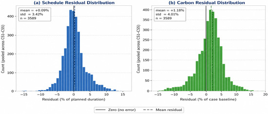
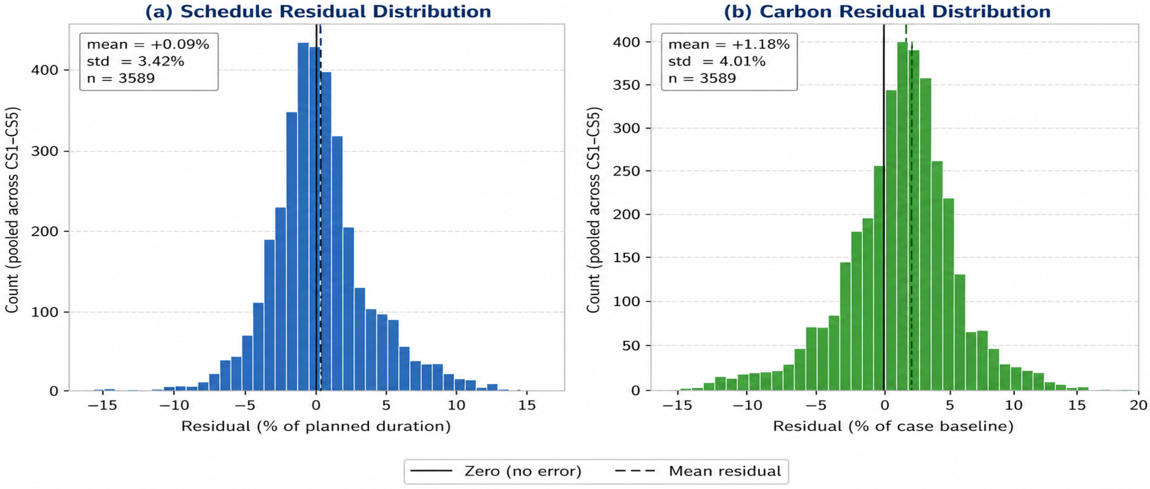
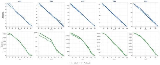
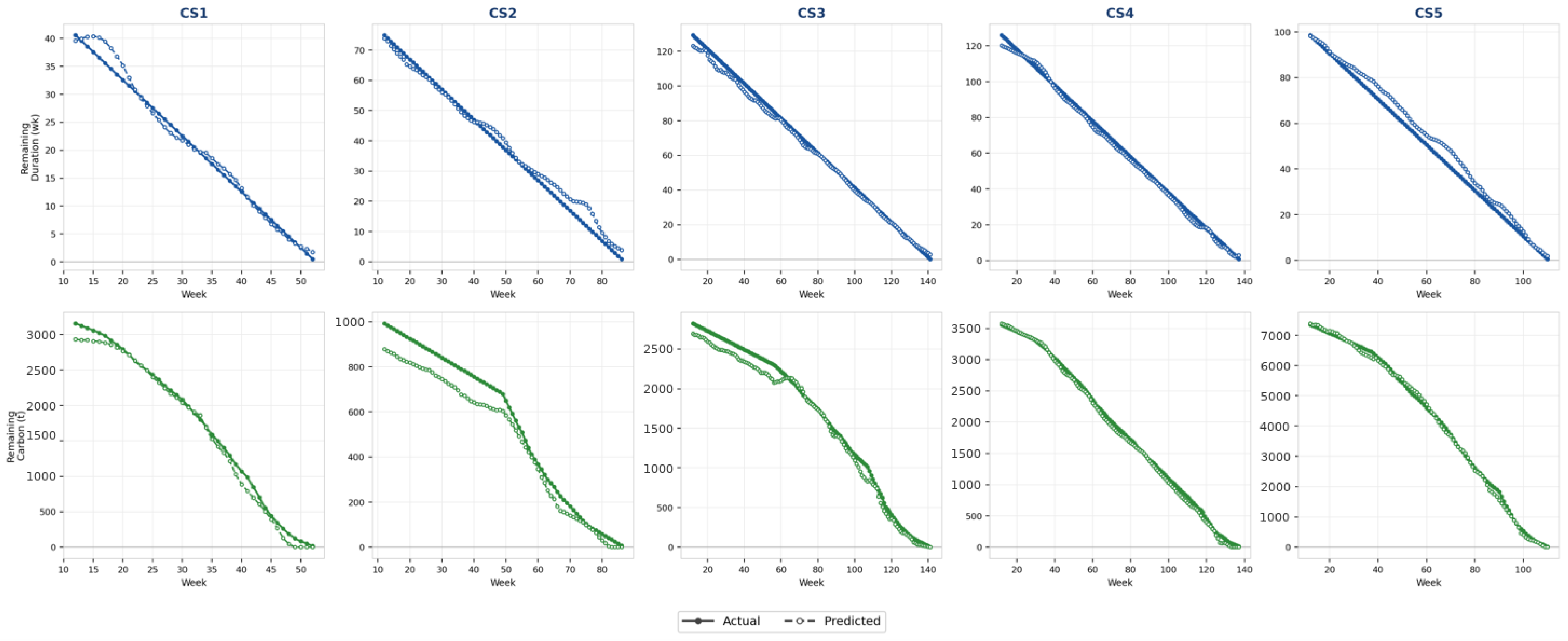
To assess whether the close tracking observed on CS1 alone reflects genuine predictive skill rather than overfitting to the simulation mechanism, the simulation mechanism rather than genuine predictive skill, Figure 5 reports the pooled residual distribution (actual − predicted) across all 3589 test windows from all five case studies, and Figure 6 extends the rolling actual-vs-predicted comparison to all five cases individually. Residuals are centered near zero for both tasks (mean = +0.09% of planned duration, +1.18% of case carbon baseline; std = 3.42% and 4.01%, respectively), with no visible systematic bias by case, indicating that prediction accuracy generalizes across building typologies rather than reflecting memorization of a single case’s synthetic data structure.

Figure 5. Pooled residual distributions (actual − predicted) across all five case studies (n = 3589 test windows): (a) schedule, (b) carbon.

Figure 6. Actual vs. predicted remaining duration (blue, top row) and remaining carbon (green, bottom row) for one representative test realization per case (CS1–CS5).

Each panel shows the LSTM-predicted remaining duration against the actual realized duration, and the Transformer-predicted remaining carbon against the actual realized carbon, tracked across weekly checkpoints for that case. Predictions use only information available up to each checkpoint week, consistent with the rolling forecast protocol applied throughout this study.

As with the cross-case validation of Table 15, all training and test data originate from the documented simulator; this constitutes evidence of architectural generalization across heterogeneous simulated configurations, not external validation against unseen real-world projects.

4.3. Monte Carlo Carbon Emission Distribution

Table 16 reports the Monte Carlo carbon emission distribution for each case study, based on the selected decision for each case (S = 10,000, Equation (9)). The 90% CI width ranges from 27 to 36% of the mean across all cases, confirming that probabilistic quantification is necessary regardless of building typology. Budget compliance probability ranges from 40% (CS4) to 63% (CS3), reflecting variation in baseline carbon intensity and material substitution potential.

Table 16. Monte Carlo Carbon Emission Distribution (CS1–CS5, S = 10,000).

Case	$\mathit{\mu }\mathit{C}$ (tCO2e)	$\mathit{\sigma }\mathit{C}$ (tCO2e)	P5 (tCO2e)	P95 (tCO2e)	CI Width	CI% of Mean	${\mathit{C}}_{\mathrm{limit}} \left(\mathit{t}\mathit{C}{\mathit{O}}_2\mathit{e}\right)$	$\mathit{P}\left(\mathit{c}\mathit{o}\mathit{m}\mathit{p}\mathit{l}\mathit{y}\right)$
CS1	2894	271	2449	3342	894	30.9%	2870	47%
CS2	813	71	698	930	233	28.6%	818	53%
CS3	2233	228	1855	2602	747	33.4%	2314	63%
CS4	3168	257	2745	3592	847	26.8%	3106	40%
CS5	6486	709	5323	7646	2323	35.8%	6679	60%

Notes: ${\mu }_C$ = mean of the Monte Carlo carbon emission distribution; ${\sigma }_C$ = standard deviation; $P_5$ and $P_{95}$ = 5th and 95th percentiles (90% confidence interval); $CI\%$ = confidence interval width as a percentage of the mean; $C_{\mathrm{l}\mathrm{i}\mathrm{m}\mathrm{i}\mathrm{t}}$ = carbon budget constraint ($0.85 \times$ B1); $P_{\mathrm{c}\mathrm{o}\mathrm{m}\mathrm{p}\mathrm{l}\mathrm{y}}$ = probability that $C_{\mathrm{t}\mathrm{o}\mathrm{t}\mathrm{a}\mathrm{l}}\le C_{\mathrm{l}\mathrm{i}\mathrm{m}\mathrm{i}\mathrm{t}}$.

4.4. NSGA-II Pareto Front Performance

Table 17 reports NSGA-II Pareto front quality indicators across all five buildings. HV (normalized against a pooled reference front from three independent search runs per case) exceeds 0.58 in all cases, and IGD remains below 0.10, confirming reasonable front coverage and convergence across typologies. The selected Pareto-optimal point for each case corresponds to λ = 0.5.

Table 17. NSGA-II Pareto Front Quality Indicators.

Case	HV (Higher Better)	IGD (Lower Better)	Pareto Schedule Range (wk)	Pareto Carbon Range (tCO2e)	Selected ${\mathit{T}}_{\mathit{o}\mathit{p}\mathit{t}}$ (wk)	Selected ${\mathit{C}}_{\mathit{o}\mathit{p}\mathit{t}}$ (tCO2e)
CS1	0.804	0.072	44.4–48.9	2321–3274	46.4	2814
CS2	0.589	0.036	73.9–84.3	801–858	79.2	820
CS3	0.822	0.035	110.4–129.5	2099–2593	115.6	2178
CS4	0.851	0.090	109.5–118.0	2790–3422	113.2	3123
CS5	0.756	0.007	92.8–103.6	5708–7741	98.8	6596

Notes: HV = Hypervolume indicator (volume of objective space dominated by the Pareto front; higher = better coverage); IGD = Inverted Generational Distance (proximity to ideal Pareto front; lower = better convergence); λ = 0.5 for all selected solutions.

4.5. Comparative Baseline Analysis

Table 18 presents comparative results across all five case studies and all four configurations, evaluated under identical pre-drawn scenario sets per configuration (common random numbers), so between-configuration differences are paired and attributable to decisions alone. Three patterns emerge. First, monitoring with manual response (B2) recovers 4.7–6.3% of the schedule but leaves carbon essentially unchanged (−0.9% to +0.1%): a descriptive DT does not decarbonize. Second, schedule-only optimization (B3) is the fastest configuration (+10.6% to +15.8%) but yields no carbon benefit and, for the timber case CS2, a 2.4% carbon increase—its equipment-dominated footprint (28% of baseline) is penalized by acceleration fuel more than it is relieved by the shorter site duration. Third, the full framework is the only configuration achieving simultaneous improvements, trading 2.7–4.6 percentage points of B3’s schedule gain for 10.4–16.4% carbon reduction. The variation in B2 and B3 effects across cases follows directly from each building’s carbon composition.

Table 18. Comparative Results Full System vs Three Baselines (CS1–CS5).

Case	Metric	B1 Static CPM	B2 Descriptive DT	B3 Schedule-Only	Full System
CS1	Duration (wk)	55.2 ± 2.5	51.9 ± 2.0	47.1 ± 2.4	48.7 ± 2.1
CS1	Carbon (tCO2e)	3424 ± 219	3427 ± 219	3428 ± 219	3067 ± 217
CS1	Sched. vs. B1	—	+6.0%	+14.6%	+11.9%
CS1	Carbon vs. B1	—	−0.1%	−0.1%	+10.4%
CS2	Duration (wk)	90.0 ± 5.8	85.8 ± 5.7	80.4 ± 5.0	84.8 ± 5.9
CS2	Carbon (tCO2e)	971 ± 51	980 ± 53	994 ± 53	825 ± 46
CS2	Sched. vs. B1	—	+4.7%	+10.6%	+5.8%
CS2	Carbon vs. B1	—	−0.9%	−2.4%	+15.0%
CS3	Duration (wk)	137.5 ± 6.2	129.0 ± 5.4	117.6 ± 5.3	122.8 ± 5.5
CS3	Carbon (tCO2e)	2774 ± 163	2786 ± 164	2800 ± 165	2318 ± 141
CS3	Sched. vs. B1	—	+6.2%	+14.4%	+10.7%
CS3	Carbon vs. B1	—	−0.4%	−0.9%	+16.4%
CS4	Duration (wk)	136.9 ± 4.5	128.3 ± 3.8	115.4 ± 3.8	118.9 ± 3.9
CS4	Carbon (tCO2e)	3699 ± 253	3709 ± 254	3715 ± 255	3256 ± 234
CS4	Sched. vs. B1	—	+6.3%	+15.8%	+13.2%
CS4	Carbon vs. B1	—	−0.3%	−0.4%	+12.0%
CS5	Duration (wk)	114.5 ± 4.9	107.8 ± 4.8	97.6 ± 4.4	102.7 ± 4.9
CS5	Carbon (tCO2e)	7844 ± 619	7840 ± 619	7825 ± 620	6721 ± 562
CS5	Sched. vs. B1	—	+5.8%	+14.8%	+10.3%
CS5	Carbon vs. B1	—	+0.1%	+0.2%	+14.3%

Notes: B1 = static CPM baseline; B2 = descriptive DT with manual acceleration response to observed progress gaps; B3 = schedule-only optimization (no carbon co-objective); Full = closed-loop DT–AI–NSGA-II framework. Values are mean ± SD over 50 execution realizations per configuration, evaluated under common random numbers. “Sched. vs. B1” is percentage improvement in expected duration; “Carbon vs. B1” is percentage reduction in expected total carbon (positive = improvement; negative for B2/B3 indicates a carbon increase).

4.6. Carbon Component Breakdown

Table 19 presents the carbon emission breakdown by component, comparing the B1 baseline against the full system across all five case studies. Site energy shows the largest relative reduction (−26% to −35%), driven jointly by shorter realized durations and site energy management. Equipment carbon falls by 14–24% through idle reduction scheduling, partially offset by acceleration fuel. Material and waste carbon fall by 8–13%, bounded by the frame-specific substitution ceilings, smallest for the already low-carbon timber structure (CS2) and largest where cementitious substitution headroom exists (CS3, CS5). Transport carbon is unchanged, as no decision variable acts on supply distances; this is a deliberate scope boundary rather than a model outcome.

Table 19. Carbon Emission Component Breakdown Full System vs B1 (CS1–CS5, tCO₂e).

Case	Component	B1	Full System	Δ%
CS1	$C_{mat}$	2954	2682	−9.2%
CS1	$C_{trans}$	28	28	0.0%
CS1	$C_{equip}$	185	159	−14.2%
CS1	$C_{waste}$	116	105	−9.1%
CS1	$C_{site}$	142	94	−33.9%
CS2	$C_{mat}$	547	504	−7.8%
CS2	$C_{trans}$	4	4	0.0%
CS2	$C_{equip}$	276	211	−23.6%
CS2	$C_{waste}$	18	17	−7.7%
CS2	$C_{site}$	126	90	−29.0%
CS3	$C_{mat}$	1983	1717	−13.4%
CS3	$C_{trans}$	11	11	0.0%
CS3	$C_{equip}$	457	360	−21.3%
CS3	$C_{waste}$	71	62	−13.2%
CS3	$C_{site}$	252	169	−33.0%
CS4	$C_{mat}$	2767	2555	−7.7%
CS4	$C_{trans}$	23	23	0.0%
CS4	$C_{equip}$	467	360	−22.9%
CS4	$C_{waste}$	110	102	−7.6%
CS4	$C_{site}$	333	217	−34.9%
CS5	$C_{mat}$	6649	5769	−13.2%
CS5	$C_{trans}$	54	54	0.0%
CS5	$C_{equip}$	384	303	−21.0%
CS5	$C_{waste}$	263	228	−13.2%
CS5	$C_{site}$	495	366	−26.0%

Notes: $C_{mat}$ denotes material embodied carbon (modules A1–A3); $C_{trans}$ represents transportation-related emissions (module A4); $C_{equip}$ corresponds to equipment fuel consumption during construction; $C_{waste}$ refers to waste disposal emissions (module A5); $C_{site}$ denotes site energy consumption. Values mean over 50 execution realizations per configuration. All carbon values are expressed in tCO₂e. Δ% is the percentage change in the Full system relative to B1$.$

4.7. DT State Evolution

Table 20 illustrates the closed-loop adaptive mechanism using one representative simulated realization per case. Recovery is triggered when the forecast overrun exceeds the 5% threshold; the system then raises acceleration to the resource cap and temporarily reduces material substitution for that has not yet started work, reverting to the planned decision after four weeks. Across the five illustrative realizations, intervention frequency varies with project scale and structure: CS3, with the longest and most activity-dense network, triggers most frequently, while CS4 did not require intervention in 200 independently simulated realizations, suggesting that its larger activity network (186 activities across 17 floors) provides more schedule float to absorb disruptions before the delay threshold is reached.

Table 20. Adaptive Recovery Events in Representative Simulated Realizations (CS1–CS5).

Case	Week	${\mathit{P}}_{\mathit{t}}$ (%)	Event
CS1	10	9.7	Recovery triggered (forecast overrun +10.1%)
CS1	51	100.0	Project complete (T = 50.3 wk)
CS2	28	21.4	Recovery triggered (forecast overrun +6.7%)
CS2	84	100.0	Project complete (T = 84.0 wk)
CS3	82	52.9	Recovery triggered (forecast overrun +5.7%)
CS3	133	100.0	Project complete (T = 132.6 wk)
CS4	—	—	No recovery triggered in 200 simulated realizations
CS4	123	100.0	Project complete on planned decision only (T = 123.4 wk)
CS5	91	86.0	Recovery triggered (forecast overrun +5.6%)
CS5	109	100.0	Project complete (T = 108.3 wk)

Notes: $P_t$ denotes the cumulative project progress at week $t$(%), $C_t$ represents the cumulative carbon emissions at week $t$ (tCO₂e), $D_{\mathrm{r}\mathrm{i}\mathrm{s}\mathrm{k}}$ is the delay risk probability predicted by the LSTM model (0–1), and $X_t^{*}$ denotes the Pareto-optimal decision vector selected at week $t$. The reported milestones are representative examples across the five case studies.

4.8. Sensitivity to Risk Parameter λ

Table 21 presents the sensitivity of the selected solution to the risk-aversion parameter λ across all five case studies, using the same Pareto front per case with λ entering only at the selection stage. The selected solution is identical across the entire range λ ∈ {0, 0.5, 1.0} in all five cases: because emission factor uncertainty is predominantly multiplicative, $\sigma C$ scales approximately with $\mu C$ along the front, and the ranking of solutions is unchanged by λ. The risk adjustment therefore functions as a conservatism margin on the reported carbon target rather than as a decision-altering preference, and the framework’s recommendations are robust to a parameter that is difficult to elicit from practitioners in advance.

Table 21. Sensitivity to Risk Parameter λ (CS1–CS5).

Case	Selected ${\mathit{T}}_{\mathit{o}\mathit{p}\mathit{t}}$ (wk)	Selected ${\mathit{C}}_{\mathit{o}\mathit{p}\mathit{t}}$ (tCO2e)	$\mathit{\sigma }\mathit{C}$ (tCO2e)	${\mathit{P}}_{\mathit{c}\mathit{o}\mathit{m}\mathit{p}\mathit{l}\mathit{y}}$
CS1	46.9	2851	274	54%
CS2	78.4	828	66	43%
CS3	116.1	2328	215	48%
CS4	112.5	3214	253	34%
CS5	98.1	6480	711	62%

Notes: These values represent the selected solution’s expected duration ($T_{opt}$), expected carbon ($C_{opt}$), carbon standard deviation (σC), and budget compliance probability ($P_{comply}$) for each case. Identical values were obtained for λ = 0.0, 0.5, and 1.0; in every case, the selection is invariant to λ over this range.

4.9. Ablation Study

Table 22 quantifies the contribution of each system component across all five buildings via closed-loop ablation (50 execution realizations per configuration, common random numbers). Removing the bi-objective optimizer is by far the most damaging ablation: carbon rises by 11.7–20.2%, and schedule lengthens by 1.2–7.9%, confirming NSGA-II as the dominant component. Removing the adaptive recovery layer (static application of the initial decision, with no forecast-triggered response) costs 0.5–1.5% of schedule while slightly lowering carbon (1.0–4.3%): the adaptive layer deliberately trades a small carbon cost for schedule recovery when delays are forecast, by temporarily relaxing material substitution for not yet started work. Removing the risk adjustment changes outcomes by at most ±3.8%, consistent with the λ-invariance established in Section 4.8.

Table 22. Ablation Study Contribution of Each System Component (CS1–CS5).

Case	Configuration	Schedule vs. Full	Carbon vs. Full
CS1	w/o NSGA-II	+6.7%	+11.7%
CS1	w/o Adaptive layer	+1.4%	−4.3%
CS1	w/o Risk adjustment	+0.5%	−1.4%
CS2	w/o NSGA-II	+1.2%	+18.7%
CS2	w/o Adaptive layer	+1.5%	−1.0%
CS2	w/o Risk adjustment	−3.8%	+2.5%
CS3	w/o NSGA-II	+5.0%	+20.2%
CS3	w/o Adaptive layer	+0.6%	−1.9%
CS3	w/o Risk adjustment	+0.7%	+0.2%
CS4	w/o NSGA-II	+7.9%	+13.9%
CS4	w/o Adaptive layer	+0.5%	−1.5%
CS4	w/o Risk adjustment	−0.1%	+0.3%
CS5	w/o NSGA-II	+5.0%	+16.6%
CS5	w/o Adaptive layer	+1.3%	−3.6%
CS5	w/o Risk adjustment	−0.2%	+0.4%

Notes: w/o = without (component removed while retaining all others). DT Loop = closed-loop feedback architecture; AI = dual-model LSTM + Transformer prediction engine; MC = Monte Carlo carbon quantification. Full system serves as reference (vs Full column). Carbon change is expressed as percentage increase relative to the full system.

4.10. Model Architecture Comparison

Table 23 compares both architectures on both tasks across all five cases. Both models achieve strong and closely comparable accuracy on each task (schedule: R² 0.965–0.991 for LSTM vs. 0.974–0.990 for Transformer; carbon: R² 0.968–0.987 for Transformer vs. 0.968–0.986 for LSTM), with neither architecture showing a decisive or consistent advantage: the better performing model on each task alternates across cases.

Table 23. Model Architecture Comparison: LSTM vs. Transformer (CS1–CS5).

Case	Model	Task	RMSE	MAPE (%)	R2	Selected
CS1	LSTM	Trem (schedule)	2.41 wk	15.8	0.965	Selected
CS1	Transformer	Trem (schedule)	2.07 wk	18.4	0.974	No
CS1	LSTM	Crem (carbon)	186.7 tCO2e	21.2	0.968	No
CS1	Transformer	Crem (carbon)	187.0 tCO2e	38.0	0.968	Selected
CS2	LSTM	Trem (schedule)	3.03 wk	17.8	0.982	Selected
CS2	Transformer	Trem (schedule)	2.87 wk	13.7	0.984	No
CS2	LSTM	Crem (carbon)	36.2 tCO2e	16.8	0.986	No
CS2	Transformer	Crem (carbon)	43.0 tCO2e	23.3	0.980	Selected
CS3	LSTM	Trem (schedule)	4.97 wk	35.8	0.982	Selected
CS3	Transformer	Trem (schedule)	5.07 wk	15.6	0.982	No
CS3	LSTM	Crem (carbon)	110.3 tCO2e	44.1	0.984	No
CS3	Transformer	Crem (carbon)	106.3 tCO2e	26.7	0.985	Selected
CS4	LSTM	Trem (schedule)	3.41 wk	9.3	0.991	Selected
CS4	Transformer	Trem (schedule)	3.81 wk	14.1	0.989	No
CS4	LSTM	Crem (carbon)	133.4 tCO2e	13.8	0.986	No
CS4	Transformer	Crem (carbon)	127.9 tCO2e	24.9	0.987	Selected
CS5	LSTM	Trem (schedule)	3.22 wk	12.0	0.988	Selected
CS5	Transformer	Trem (schedule)	3.05 wk	9.4	0.990	No
CS5	LSTM	Crem (carbon)	358.6 tCO2e	19.1	0.978	No
CS5	Transformer	Crem (carbon)	343.9 tCO2e	30.9	0.980	Selected

Notes: Each model was trained and evaluated on the identical dataset partition. RMSE in weeks for schedule tasks; RMSE in tCO₂e for carbon tasks. Selected = model assigned to this task in the dual-model architecture, retained for complementary capability rather than a consistent accuracy advantage.

The task-specific assignment is therefore retained not for a raw accuracy advantage but for complementary capabilities: the LSTM head natively supports the delay risk classification output required by the risk-informed loop (AUC 0.834–0.948), while the Transformer’s attention mechanism scales more directly to the longer, feature-weighted carbon-accrual sequences used across the larger case studies.

5. Discussion

The results consistently confirm that the closed-loop DT framework outperforms all three baseline configurations across all five case studies, achieving concurrent schedule and carbon improvements that no single-component architecture could replicate. The following subsections interpret these findings in relation to existing literature, assess the contribution of each architectural component, and identify the principal limitations and directions for future research.

5.1. Schedule and Carbon Performance: Beyond Static Planning

The schedule improvements (5.8–13.2% across five case studies) and carbon reductions (10.4–16.4%) directly address the execution failures attributed to static planning tools [2,3,4]. The framework achieves this through adaptive feedback under weekly re-evaluation, a capability that static BIM-based approaches [10,11] cannot provide by design. For CS1, the carbon outcome of 426 kgCO₂e/m² remains below the RIBA 2030 interim target [40] and the European embodied carbon benchmark of Le Den et al. [41], demonstrating that execution-phase optimization alone can contribute meaningfully to decarbonization targets without requiring design-phase changes. The comparison with B3 reveals a counterintuitive finding: schedule-only optimization worsens carbon performance relative to the full framework across all five case studies (B3 carbon exceeds the full framework by 11.8–20.8%), as NSGA-II without a carbon co-objective selects a resource-intensive fast-tracking strategy. This reinforces the need for genuinely bi-objective formulations absent from prior construction optimization work [16,17].

5.2. Probabilistic Carbon Modeling

The 90% confidence interval width of 27–36% of the mean across all five case studies extends the finding of Huang and Wang [18] (8.85% CI expansion) to a dynamically re-evaluated scheduling context, reflecting uncertainty compounding across all five carbon components under weekly re-planning. The deterministic baseline lies near the upper tail of the optimized distribution for CS1; the B1 value falls approximately two standard deviations above the full system’s expected carbon, indicating that deterministic models may misrepresent carbon risk exposure, causing project teams to abandon feasible targets prematurely. The probabilistic compliance probability metric introduced here is unavailable under the deterministic approaches of Hammond and Jones [19] or the design-phase framework of Amro and Naimi [20].

5.3. AI Architecture and Ablation

Ablation results show highly unequal component contributions. Removing the bi-objective optimizer produces by far the largest carbon increase (11.7–20.2%) and a schedule cost of 1.2–7.9%, confirming NSGA-II as the dominant architectural component. Removing the adaptive recovery layer and applying the initial decision statically with no forecast-triggered response costs only 0.5–1.5% of schedule while slightly reducing carbon (1.0–4.3%), since the adaptive layer deliberately trades a small carbon cost for schedule recovery when delays are forecast. Removing risk adjustment changes outcomes by at most ±3.8%, consistent with the λ-invariance. The optimizer is therefore the primary driver of the framework’s performance, with the adaptive and risk adjustment layers contributing smaller, more specialized value: schedule resilience under disruption and conservatism margin reporting, respectively, reinforcing the value of the integrated architecture over the optimizer alone [12,16,17].

5.4. Positioning Relative to Prior DT Frameworks

The framework addresses the three principal limitations of Pan and Zhang [9]: replacing near-term extrapolation with deep sequential forecasting, adding probabilistic carbon modeling consistent with EN 15978 [21], and embedding a continuously updated Pareto front within the DT feedback loop. The improvements beyond B2 (descriptive DT) quantify the prescriptive DT performance premium, a gap identified qualitatively in prior reviews [7,8] but not previously measured. This study demonstrates that construction DTs can transition from passive monitoring tools to active, risk-informed decision-making systems, enabling simultaneous schedule and carbon improvements unavailable under static planning approaches. This finding is consistent with concurrent advances in AI-driven BIM-based construction management; Amro et al. [42] demonstrated comparable integration of scheduling, risk, and sustainability optimization within a BIM-enabled AI framework, reinforcing the broader trajectory toward adaptive, data-driven construction execution systems.

5.5. Practical Implementation and Scalability

The computational budget of the framework is modest: on a single CPU core, one NSGA-II planning run (48 × 50 evaluations over 24 scenarios) completes in 10–20 s per case, one Monte Carlo quantification (S = 10,000) in 1–3 s, and the full five-case, four-configuration closed-loop evaluation in under one minute; per-case model training completes in minutes with the compact architectures. Weekly re-planning is therefore feasible on commodity hardware even for the largest network studied (186 activities, CS4), and the vectorized CPM evaluation scales linearly in activities and scenarios. Deployment effort concentrates elsewhere: mapping BIM quantities and activity networks into the state model, establishing reliable progress and energy data flows from site systems of heterogeneous quality, and integrating recommendations into established planning workflows. Organizational barriers, including procurement lead times for substituted materials, contractual restrictions on resequencing, and practitioner acceptance of algorithmic re-planning, are at least as binding as technical ones; the framework is accordingly positioned as decision support, with the weekly Pareto front and compliance probability presented to, not substituted for, the project team. The methodology is not Europe-specific: transferring requires regional emission factors, local supply distances, and locally calibrated duration variability and disruption rates, all of which are exposed as explicit parameters; validation on non-European and infrastructure projects remains future work.

5.6. Limitations

Sensor and reporting noise is represented only through a stylized autoregressive observation model; real telemetry artifacts such as dropouts, drift, and systematic bias are not modeled and represent a core methodological constraint. IoT deviation streams are synthetic and may not capture real site autocorrelation. Validation is limited to five European buildings; infrastructure and non-European typologies remain untested. NSGA-II hyperparameters were not tuned per building type. Emission factors are time-invariant within each simulated project but vary stochastically across projects to represent supplier-level differences; temporal drift in supplier emission factors within a single project is not modeled. Monte Carlo–dropout prediction intervals were under-covered relative to their nominal target (empirical coverage 59–69% against a 90% target), so the framework’s forecast uncertainty is understated. Tree ensemble benchmarks (Random Forest, XGBoost) proved competitive with the neural prediction engine on both within-case and cross-case regression, indicating that lighter-weight alternatives may suffice where native sequence handling and risk classification are not required. All generalization evidence, including cross-case transfer, derives from the documented simulator; it demonstrates robustness across heterogeneous project configurations rather than field-level external validity, since the framework has not been evaluated under continuously evolving field conditions involving sensor failures, missing data, changing project constraints, or contractor decision-making. Future implementations should replace synthetic IoT streams with real-site observations; emerging remote sensing technologies such as UAV-based inspection [43] represent a promising avenue for higher-fidelity data acquisition in construction DT deployments.

6. Conclusions

This study developed and evaluated, as a simulation-based proof of concept, a risk-informed closed-loop Digital Twin framework for the simultaneous optimization of construction scheduling and pre-use embodied carbon (A1–A5) under uncertainty. The framework integrates a formalized DT state transition model, a dual deep learning prediction engine, Monte Carlo-based probabilistic carbon quantification, and risk-adjusted NSGA-II optimization within a closed weekly decision loop, evaluated across five European case studies anchored to published project data.

Under a fully documented and reproducible simulation benchmark, the full framework achieved simultaneous schedule improvements of 5.8–13.2% and embodied carbon reductions of 10.4–16.4% relative to a static Critical Path Method baseline; for the primary case study (CS1), mean carbon intensity fell from 476 to 426 kgCO₂e/m². Ablation analysis identifies the bi-objective optimizer as the dominant contributor (an 11.7–20.2% carbon increase when removed), with the adaptive recovery layer contributing schedule resilience under disruption and risk adjustment contributing a conservatism margin on the reported carbon target, the latter consistent with the selected solution’s invariance to the risk-aversion parameter λ. The contribution of this work is not the individual components Digital Twins, LSTM and Transformer networks, Monte Carlo methods, and NSGA-II- which are all established techniques, but their systematic, fully transparent integration into a unified decision loop, together with a reproducible benchmark against classical and ablated alternatives, including competitive tree ensemble baselines.

The framework preliminarily validates this integrated approach in simulation; it does not demonstrate field performance. Future research should prioritize: (i) deployment on an instrumented project with live BIM–IoT streams to replace the synthetic observation model, with UAV-based inspection [43] as a candidate high-fidelity acquisition channel; (ii) extension to operational carbon (Modules B6–B7) and coupling with dynamic, supplier-specific Environmental Product Declarations; (iii) calibrated uncertainty quantification and comparative evaluation against NSGA-III and MOEA/D; and (iv) validation on non-European and infrastructure typologies.

References

- UNEP; GlobalABC. Global Status Report for Buildings and Construction 2024/2025; UNEP: Nairobi, Kenya, 2025; Available online: https://www.unep.org/resources/report/global-status-report-buildings-and-construction-20242025 (accessed on 5 May 2026).
- Changali; Sriram; Mohammad, A.; van Nieuwland, M. The construction productivity imperative. McKinsey Q. 2015, pp. 1–10. Available online: https://www.mckinsey.com/capabilities/operations/our-insights/the-construction-productivity-imperative (accessed on 5 May 2026).
- McKinsey and Company. Seize the Decade: Maximizing Value Through Preconstruction Excellence, McKinsey Capital Projects and Infrastructure. August 2024. Available online: https://www.mckinsey.com/capabilities/operations/our-insights/seize-the-decade-maximizing-value-through-pre-construction-excellence (accessed on 5 May 2026).
- CoST; World Bank. Drivers of Infrastructure Delays: What Can 480 Projects Across Three Continents Teach Us? Infrastructuretransparency.org. May 2025. Available online: https://infrastructuretransparency.org/2025/05/20/drivers-of-infrastructure-delays/ (accessed on 5 May 2026).
- Barbosa; Filipe; Woetzel, J.; Mischke, J. Reinventing Construction. In Reinventing Construction: A Route to Higher Productivity; MCKinsey Global Institute: Washington, DC, USA, 2017. [Google Scholar]
- Tao, F.; Zhang, H.; Liu, A.; Nee, A.Y. Digital twin in industry: State-of-the-art. IEEE Trans. Ind. Inform. 2018, 15, 2405–2415. [Google Scholar] [CrossRef] [Scilit]
- Hosamo, H.H.; Imran, A.; Cardenas-Cartagena, J.; Svennevig, P.R.; Svidt, K.; Nielsen, H.K. A review of the digital twin technology in the AEC-FM industry. Adv. Civ. Eng. 2022, 2022, 2185170. [Google Scholar] [CrossRef] [Scilit]
- Lu, Y.; Liu, C.; Kevin, I.; Wang, K.; Huang, H.; Xu, X. Digital Twin-driven smart manufacturing: Connotation, reference model, applications and research issues. Robot. Comput.-Integr. Manuf. 2020, 61, 101837. [Google Scholar] [CrossRef] [Scilit]
- Pan, Y.; Zhang, L. A BIM-data mining integrated digital twin framework for advanced project management. Autom. Constr. 2021, 124, 103564. [Google Scholar] [CrossRef] [Scilit]
- Sacks, R.; Eastman, C.; Lee, G.; Teicholz, P. BIM Handbook: A Guide to Building Information Modeling for Owners, Designers, Engineers, Contractors, and Facility Managers; John Wiley & Sons: Hoboken, NJ, USA, 2018. [Google Scholar]
- Eastman, C.M. BIM Handbook: A Guide to Building Information Modeling for Owners, Managers, Designers, Engineers and Contractors; John Wiley & Sons: Hoboken, NJ, USA, 2011. [Google Scholar]
- Gondia, A.; Siam, A.; El-Dakhakhni, W.; Nassar, A.H. Machine learning algorithms for construction projects delay risk prediction. J. Constr. Eng. Manag. 2020, 146, 04019085. [Google Scholar] [CrossRef] [Scilit]
- Laura-Portugal, C.; Hammad, A. Deep learning-based forecasting for construction project duration at completion. Int. J. Constr. Manag. 2026, 26, 1543–1561. [Google Scholar]
- Oliveira, H.S.; Oliveira, H.P. Transformers for energy forecast. Sensors 2023, 23, 6840. [Google Scholar] [CrossRef] [Scilit] [PubMed]
- Shi, T.; Shide, K. A comparative analysis of LSTM, GRU, and Transformer models for construction cost prediction with multidimensional feature integration. J. Asian Archit. Build. Eng. 2026, 25, 634–649. [Google Scholar]
- Deb, K.; Pratap, A.; Agarwal, S.; Meyarivan, T.A. A fast and elitist multiobjective genetic algorithm: NSGA-II. IEEE Trans. Evol. Comput. 2002, 6, 182–197. [Google Scholar] [CrossRef] [Scilit]
- Soni, S.; Chauhan, M.; Singh, P.; Agarwal, A.K.; Sharma, K. Optimizing construction time, cost, and quality: A hybrid AHP-NSGA-II optimization model. Asian J. Civ. Eng. 2024, 25, 4053–4067. [Google Scholar] [CrossRef] [Scilit]
- Huang, W.; Wang, W.C. Uncertainty analysis framework for carbon emissions in building materialization phase using an improved statistical–data quality indicator hybrid method. Energy Build. 2025, 349, 116457. [Google Scholar] [CrossRef] [Scilit]
- Hammond, G.P.; Jones, C.I. Embodied energy and carbon in construction materials. Proc. Inst. Civ. Eng.-Energy 2008, 161, 87–98. [Google Scholar] [CrossRef] [Scilit]
- Amro, S.O.; Naimi, S. Symmetry-Based Structural Optimization of 50 Dutch Buildings: Quantitative Framework for Material and Carbon Reduction. Buildings 2025, 15, 3962. [Google Scholar] [CrossRef] [Scilit]
- EN 15978:2011; Sustainability of Construction Works Assessment of Environmental Performance of Buildings Calculation Method. CEN: Brussels, Belgium, 2011.
- Wang, Q.; Xu, X.; Ding, X.; Chen, T.; Deng, R.; Li, J.; Jiang, J. Multi objective optimization and evaluation approach of prefabricated component combination solutions using NSGA-II and simulated annealing optimized projection pursuit method. Sci. Rep. 2024, 14, 16688. [Google Scholar] [CrossRef] [Scilit] [PubMed]
- Hochreiter, S.; Schmidhuber, J. Long short-term memory. Neural Comput. 1997, 9, 1735–1780. [Google Scholar] [CrossRef] [Scilit] [PubMed]
- Vaswani, A.; Shazeer, N.; Parmar, N.; Uszkoreit, J.; Jones, L.; Gomez, A.N.; Kaiser, Ł.; Polosukhin, I. Attention is all you need. In Advances in Neural Information Processing Systems; NIPS Foundation: San Diego, CA, USA, 2017; Volume 30. [Google Scholar]
- UK Department for Energy Security and Net Zero (DESNZ). Greenhouse Gas Reporting: Conversion Factors 2024; DESNZ: London, UK, 2024. Available online: https://www.gov.uk/government/publications/greenhouse-gas-reporting-conversion-factors-2024 (accessed on 5 May 2026).
- Intergovernmental Panel on Climate Change (IPCC). 2006 IPCC Guidelines for National Greenhouse Gas Inventories; Institute for Global Environmental Strategies: Hayama, Kanagawa, Japan, 2006. [Google Scholar]
- Wernet, G.; Bauer, C.; Steubing, B.; Reinhard, J.; Moreno-Ruiz, E.; Weidema, B. The ecoinvent database version 3 (part I): Overview and methodology. Int. J. Life Cycle Assess. 2016, 21, 1218–1230. [Google Scholar] [CrossRef] [Scilit]
- Ballesteros-Pérez, P.; Cerezo-Narváez, A.; Otero-Mateo, M.; Pastor-Fernández, A.; Zhang, J.; Vanhoucke, M. Forecasting the project duration average and standard deviation from deterministic schedule information. Appl. Sci. 2020, 10, 654. [Google Scholar] [CrossRef] [Scilit]
- Thiele, B.; Ryan, M.; Abbasi, A. Developing a dataset of real projects for portfolio, program and project control management research. Data Brief 2021, 34, 106659. [Google Scholar] [CrossRef] [Scilit] [PubMed]
- Usmanov, V. Synthetic Data Generation Methodology for Construction Machinery Assembly Optimization. Buildings 2025, 15, 4176. [Google Scholar] [CrossRef] [Scilit]
- Benke, B.; Chafart, M.; Shen, Y.; Ashtiani, M.; Carlisle, S.; Simonen, K. A Harmonized Dataset of High-Resolution Embodied Life Cycle Assessment Results for Buildings in North America. Sci. Data 2025, 12, 1085. [Google Scholar] [CrossRef] [Scilit] [PubMed]
- Hammond, G.P.; Jones, C.I. Inventory of Carbon and Energy (ICE) Database, Version 3.0; Circular Ecology/University of Bath: Bath, UK, 2019; Available online: https://circularecology.com/embodied-carbon-footprint-database.html (accessed on 5 May 2026).
- EN 16258:2012; Methodology for Calculation and Declaration of Energy Consumption and GHG Emissions of Transport Services (Freight and Passengers). CEN: Brussels, Belgium, 2012.
- UK Green Building Council (UKGBC). The Enterprise Centre Case Study; UKGBC: London, UK, 2016. Available online: https://ukgbc.org/resources/the-enterprise-centre/ (accessed on 5 May 2026).
- Waugh Thistleton Architects. 6 Orsman Road Project Documentation, London. 2020. Available online: https://waughthistleton.com/project/orsman/ (accessed on 5 May 2026).
- London Energy Transformation Initiative (LETI). LETI Embodied Carbon Primer; LETI: London, UK, 2020; Available online: https://www.leti.london (accessed on 5 May 2026).
- Eiffage Construction. The Hypérion Adventure Begins: Eiffage Immobilier Launches the Construction of the Tallest Wooden Residential Tower in France. 2019. Available online: https://www.eiffage.com/en/media/news/the-hyperion-adventure-begins-eiffage-immobilier-launches-the-construction-of-the-tallest-wooden-residential-tower-in-france (accessed on 5 May 2026).
- Cundall. Three Chamberlain Square, Paradise Birmingham Project Case Study, Birmingham. 2025. Available online: https://www.cundall.com/projects/three-chamberlain-square-paradise-birmingham (accessed on 5 May 2026).
- Röck, M.; Sorensen, A.; Balouktsi, M.; Ruschi Mendes Saade, M.; Rasmussen, F.N.; Birgisdottir, H.; Frischknecht, R.; Lützkendorf, T.; Hoxha, E.; Habert, G.; et al. Global Buildings Database Seed on Whole Life Carbon Emissions, Energy Performance, and Material Intensity (GBDB CarbEnMats); Zenodo: Geneva, Switzerkand, 2024. [Google Scholar] [CrossRef]
- Royal Institute of British Architects (RIBA). RIBA 2030 Climate Challenge, 2nd ed.; RIBA: London, UK, 2021; Available online: https://www.architecture.com/about/policy/climate-action/2030-climate-challenge (accessed on 5 May 2026).
- Le Den, X.; Steinmann, J.; Röck, M.; Birgisdottir, H.; Horup, L.H.; Tozan, B.; Sørensen, A. Towards Embodied Carbon Benchmarks for Buildings in Europe—Summary Report; Zenodo: Geneva, Switzerkand, 2022. [Google Scholar] [CrossRef]
- Amro, S.O.A.; Naimi, S.; Ibrahim, A.A. AI-Driven Optimization of Scheduling, Risk, and Sustainability in BIM-Enabled Construction Project Management. In Arabian Journal for Science and Engineering; Springer: Berlin/Heidelberg, Germany, 2026. [Google Scholar] [CrossRef] [Scilit]
- Aburqaq, I.S.A.; Naimi, S.; Saedi, S.; Shahin, M.A.A. Assessment of UAV Usage for Flexible Pavement Inspection Using GCPs: Case Study on Palestinian Urban Road. Sustainability 2025, 17, 8129. [Google Scholar] [CrossRef] [Scilit]
Disclaimer/Publisher’s Note: The statements, opinions and data contained in all publications are solely those of the individual author(s) and contributor(s) and not of MDPI and/or the editor(s). MDPI and/or the editor(s) disclaim responsibility for any injury to people or property resulting from any ideas, methods, instructions or products referred to in the content. |
© 2026 by the authors. Licensee MDPI, Basel, Switzerland. This article is an open access article distributed under the terms and conditions of the Creative Commons Attribution (CC BY) license.