A Tool for Carbon Farming Combining Soil Organic Carbon Modelling and Agricultural Decision Support Systems: Adapting the RothC Model to Simulate DSS Informed Agricultural Practices in a Mediterranean Climate

Abstract

Decision support systems (DSSs) help farmers and decision-makers to find cropping systems which increase productivity while decreasing the use of fertilizers and irrigation; however, few DSSs exist which integrate soil carbon models, especially in Mediterranean climate. Here, we test whether RothC20_N, a version of the widely used RothC model adapted for Mediterranean and arid climates, can estimate the soil water content (SWC), soil organic carbon (SOC), and soil respiration (Rs), observed in two different cropping systems, one traditional and the other informed by the DSS by Horta Srl. The model was calibrated and tested against two long-term (8 years) field experiments in two different areas in Italy. The two sites showed characteristically dry soils during the summer period; RothC20_N was able to predict correctly the soil water content time series observed in both sites. RothC20_N could predict the measured SOC and heterotrophic respiration time series with Nash–Sutcliff efficiency ~0.3, normalized root mean squared error ~0.4, and Kling–Gupta efficiency > 0. This study shows that the multi-objective calibrated RothC20_N is an interesting candidate for inclusion in a DSS to broaden the potential of the DSS to increase the sustainability of agricultural practices by also addressing soil carbon dynamics while maintaining high agricultural productivity.

1. Introduction

Soils in Mediterranean climatic zones are often depleted in soil organic carbon (SOC; [1]); this can be seen as an opportunity for the sequestration of carbon into the soil using focused agricultural practices [2]. Soil is both a sink and a source of CO₂ due to anthropogenic and natural drivers [3]; as such, agriculture can also be a source or a sink of CO₂, depending on the cropping system used and the conditions in which it is deployed [4]. There are many agricultural practices with the potential to increase SOC (referred to as soil carbon sequestration practices); among them are the use of cover crops, reduced tillage, green mulching, etc. [5,6,7]. Turning agricultural soils into net sinks of CO₂ is fundamental to reach carbon neutrality and maintain the global temperature rise within 1.5 °C [8], while also avoiding food shortages. As such, it is important to develop decision support systems (DSSs) aimed at soil carbon sequestration to help policy makers and farmers estimate and verify which practices are best suited to increase SOC and reduce greenhouse gases emissions, without affecting food production [9].

Carbon enters the soil as organic matter and is then degraded by the soil microorganisms, resulting in the emission of CO₂ from the soil [10]; SOC can thus be increased by increasing the input of organic matter and/or decreasing the rate of its degradation to CO₂ (a process here referred to as mineralization [11,12]). The total flow of CO₂ exiting from the soil is called soil respiration ($R_s$) and can be thought as the sum of the respiration by autotrophic organisms ($R_a$, mostly plant roots) and the respiration by heterotrophic organisms ($R_h$, mostly microbes and fungi in the soil degrading dead organic matter [13]). Every agricultural practice aimed at increasing SOC should study both soil inputs and outputs: some studies show that increasing the input of organic matter to the soil, for example, can result in a net increase in soil CO₂ emissions [14,15]. Soil carbon and soil respiration can be directly measured in the field [16]; however, soil organic carbon pools are affected by large uncertainties and need measurement intervals of at least 5–10 years to detect statistically significant trends in SOC, while $R_s$ measurements are, in general, very expensive [17]. Measurements of SOC and $R_s$ are important to assess and verify the effect of different cropping systems on SOC, but not to predict possible future SOC changes related to the use of a certain cropping system.

Soil carbon sequestration practices increase SOC by increasing the input of organic matter in the soil, reducing the degradation of SOC, or both [18]. Cover crops, typically, decrease the time the bare soil is exposed to the elements, reducing soil erosion and SOC degradation; moreover, when incorporated into the soil, they result in a large increase in carbon inputs to the soil [19]. Reduced tillage has the potential of decreasing SOC degradation by avoiding the exposure of the lower soil to the elements and reducing the disturbance of the soil structure [20]. The efficacy of soil carbon sequestration practices changes depending on the type of soil on which they are applied. Vertisols, soils with relatively high clay content and often showing deep cracks forming in dry periods, have usually already high percentages of SOC protected by the clay fraction: in this case, soil sequestration practices should focus on the decrease in the degradation of SOC [21]. Inceptisols, young soils with moderate development, may vary greatly in their properties; recent studies show that a combination of increased carbon inputs (with diversified cropping systems) and decreased soil disturbance (with reduced tillage) have the potential of increasing SOC in inceptisols [22,23].

Soil carbon models are aimed at predicting SOC changes and $R_h$ emissions [24]; they can be both empirical (based on statistical analysis of existing SOC datasets) or mechanistic (trying to represent the processes involved in soil carbon dynamics). A widely used empirical model is that formulated in the IPCC (Internation Panel for Climate Change) national GHG (greenhouse gases) inventory guidelines (Tier 1), which estimates broad, general SOC trends in a certain climate, soil, and management combination [25]. Mechanistic models are usually based on the concept of different soil organic matter pools decaying exponentially at different rates depending on soil conditions (temperature, water content, etc.) and on soil management practices (crop rotation, tillage, etc.). Different models vary in their robustness, geographical area of applicability, number of processes represented, and amount of data required; however, the use of soil carbon models is still mostly restricted to research studies.

A promising way to use soil carbon models to inform policy makers and farmers’ decisions is to integrate them into DSSs [17]. DSSs are already used in agriculture to increase efficiency by decreasing irrigation, fertilization, and the application of pesticides [26]. Most of the existing DSSs aimed at soil carbon estimation employ empirical models (e.g., IPCC Tier 1 method [17,27]). However, some DSSs integrated with mechanistic models exist, for example, the USA COMET-Farm integrated with the DayCent model [28], or the FullCAM model, used in Australia’s National Greenhouse Gas Accounts [29], integrated with the RothC model.

The example of FullCAM is particularly interesting: here, a soil carbon sub-model (RothC) is integrated with a plant litter sub-model and a vegetation growth sub-model to predict carbon fluxes due to various types of land managements in Australia [30]. The RothC model is one of the most used soil carbon dynamic models, with a simple design and low requirement of data [31,32]. RothC models only the carbon fluxes in the soil, with no sub-model for plant growth; it modifies the decay rate of the carbon pools depending on air temperature, soil water content (modelled with a simple bucket model for water balance), and presence/absence of vegetation. As such, RothC can be easily integrated into a DSS which already models vegetation physiology, soil temperature, and agricultural practices [33].

Even if RothC can be considered a mechanistic model, it still uses empirical relationships to estimate the effects of the soil conditions of SOC dynamics; therefore, these relationships have to be adapted to various different conditions around the world with different approaches [33,34]. For example, due to the reported limitations of RothC in estimating SOC dynamics in semi-arid regions [35], Farina et al. [36] developed a modified version of RothC, called RothC20_N, modifying the soil water balance bucket model of RothC and the effects of low soil water content on SOC pool mineralization. RothC20_N successfully simulated the SOC data collected in five long-term (12–100 years duration) field experiments in semi-arid areas [36].

Another problem of the RothC model is its over-parametrization, which leads to equifinality [37], meaning that different sets of parameter values can give the same results for SOC projections, thus decreasing the reliability of the model. Cagnarini et al. [38] have shown that RothC’s equifinality problem can be minimized by conducting a multi-objective calibration: instead of using only SOC data as a target for calibration, multiple time series of relevant soil variables should be used to constrain the model parameters. In particular, the use of soil water content time series can help in the calibration of the soil water balance sub-model [39], and it has been shown that $R_s$ time series, once partitioned into its $R_a$ and $R_h$ components, can yield reliable RothC calibration with only 3 years of data [40,41].

RothC20_N seems, thus, a promising carbon model to integrate into agricultural DSSs aimed at Mediterranean (and semi-arid) conditions, to estimate changes in SOC dynamics due to the adoption of the DSS. However, the model should be able, after proper, multi-objective calibration, to simulate the different SOC dynamics in a certain area, when DSSs informed cropping systems are applied, with respect to a cropping system managed traditionally, without the use of the DSS. Here, we hypothesize that RothC20_N can successfully estimate the difference in SOC dynamics in a field when the cropping system is informed by a DSS, with respect to a field with no use of DSS, in Mediterranean climate.

To test this hypothesis, our objectives were to (a) analyse the difference in soil organic carbon, soil respiration, and other variables related to carbon fluxes, between two different cropping systems, a traditional cropping system not using the DSS (here referred to as conventional cropping system, CCS) and a DSS informed cropping system (here referred to as efficient cropping system, ECS), in two long-term (8 years) field studies in different parts of Italy; (b) use a multi-objective calibration for RothC20_N and assess the level of agreement between model estimates and measurements in the two cropping systems, in the two areas. Integrating a validated SOC model with a DSS would greatly help farmers in mediterranean and semi-arid climates to explore options to increase yields and decrease use of water, fertilizers, and pesticides, while also maintaining or increasing SOC levels.

2. Materials and Methods

2.1. Field Sites

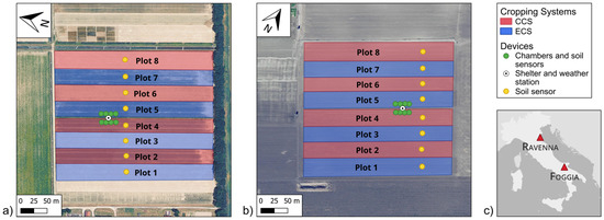
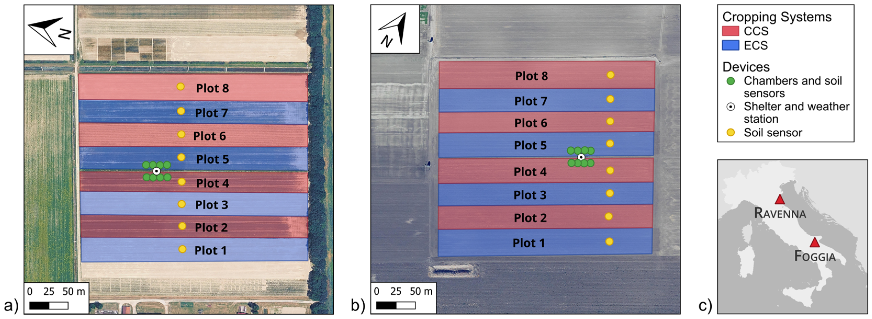
Two field experiments were set up at experimental farms in Ravenna province (locality of Cà Bosco; 44°29′15” N, 12°10′44” E, experimental area 7 hectares) and in Foggia province (locality of San Giuseppe; 41°29′27” N, 15°30′14” E, experimental area 7.5 hectares), as shown in Figure 1. The two sites differ in soil type, water regime, climate, and land use; their differences are meant to assure that the study results are representative for most conditions found in Italy. The Ravenna site is characterized by the following: silty clay loam inceptisol in the west side and silty loam inceptisol in the east side; 4 m elevation above mean sea level (a.m.s.l.); flat landscape; humid sub-tropical climate (Cfa by Köppen–Geiger classification, [42]), with mean yearly temperature of 14.3 °C, cumulative annual rainfall of 659 mm, rain events concentrated in spring and fall, thermic soil temperature regime, and Ustic soil water content regime. The Foggia site is characterized by the following: silty clay loam vertisol; 70 m elevation a.m.s.l.; flat landscape; cold semi-arid climate (BSk by Köppen–Geiger [43]), with mean yearly temperature of 16.9 °C and cumulative annual rainfall of 554 mm, thermic soil temperature regime, and Xeric soil water content regime. More information on the experimental sites can be found in the Supplementary Materials.

Figure 1. Plots and cropping systems’ subdivision into plots, with the equipped devices (soil temperature sensors, soil gas chambers, and weather station), for the two experimental fields in (a) Ravenna and (b) Foggia; (c) the location of the experimental farms in Italy. Each map in (a,b) shows the north direction (top-left arrow) and the map scale (bottom-left). Each soil gas chamber was equipped with its own soil temperature and soil water content sensors for the correct interpretation of soil gas fluxes. Satellite images: © Copernicus 2026.

2.2. Field Experiment Setup and Cropping Systems Applied

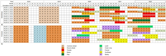
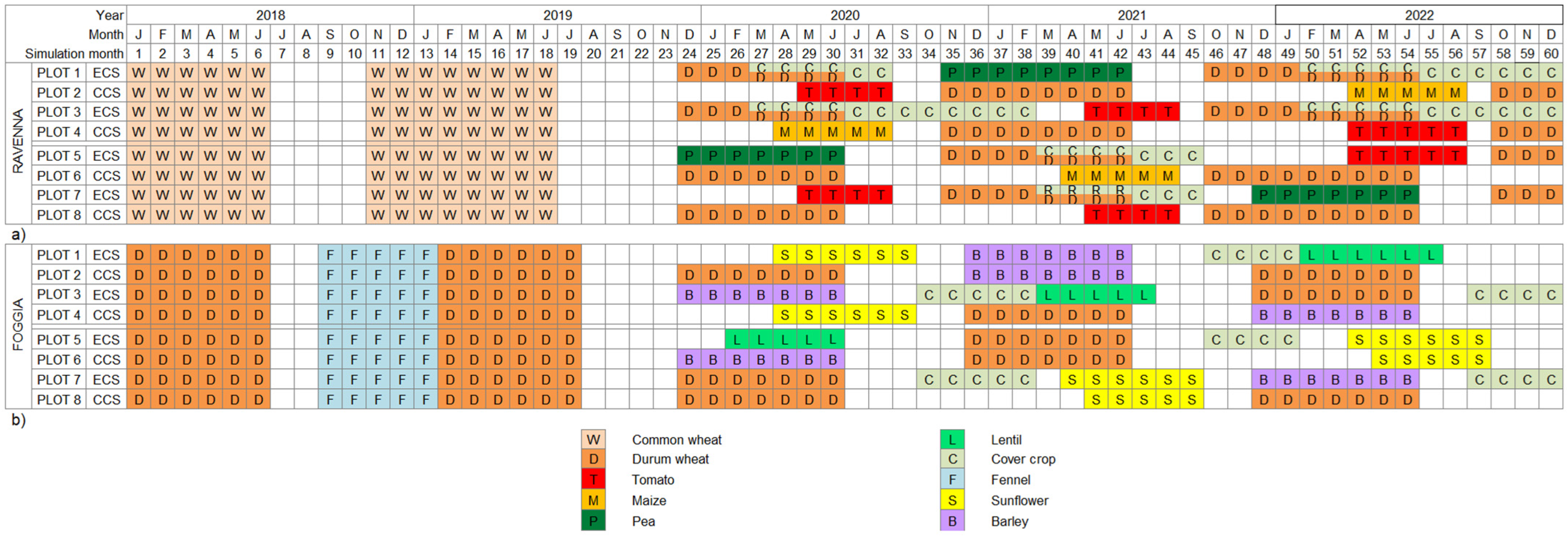
The field experiments were setup and managed by Horta Srl as part of the experimental fields of the EU LIFE Project for Agricultural GReenhouse gases EmiSsions Through Innovative Cropping systems (Agrestic, https://www.agrestic.eu/en/, accessed on 14 May 2025), with the objective of promoting the adoption of regenerative agricultural practices aimed at mitigating climate change by decreasing emissions from the soil to the atmosphere and increasing soil organic carbon. The experimental sites were used to compare two cropping systems arranged in 8 plots (Figure 1): Conventional Cropping System (CCS) and Efficient Cropping System (ECS); CCS uses fertilizers, pesticides, irrigation, and soil tillage in line with the practices generally followed in the surrounding farms; ECS uses fertilizers, pesticides, irrigation, and seeding density as suggested by a dedicated web-based Decision Support System (DSS by Horta Srl, version from 2019), with nitrogen-fixing crops/legumes and cover crops included and managed under expert agronomist advice. The arrangement of the field experiments and the details of crop sequence are summarised in Figure 2.

Figure 2. Cropping systems, CCS and ECS, used in the (a) Ravenna and (b) Foggia experimental sites, for the first 5 years of the experiment. The whole 8 years are shown in the Supplementary Materials.

The same management was used for both ECS and CCS and both experimental sites during the first period (January 2018 to June 2019); this was carried out to standardize the starting conditions of the experiment and to test the hypothesis that measurements from ECS and CCS are comparable when the two cropping systems are kept equal, on the same experimental site. Since December 2019, the two cropping systems diverge, with the ECS cropping system being informed by the DSS; the inputs required by the DSS are agronomic and soil data, which are analysed by several process-based models (e.g., a phenological model, [44,45]; a hydrological model [46]; etc.); the DSS outputs are agronomic advices concerning irrigation, fertilization, and tillage practices [47,48] (a description of the agricultural practices for the cropping systems can be found in the Supplementary Materials, Tables S1–S4).

Apart from the use of a different crop rotation and the use of cover crops, the DSS affected the amount of tillage events, the total amount of water, and the total amount of fertilizers applied in ECS with respect to CCS: 33 tillage events instead of 41, 944 mm of irrigation with respect to 1296 mm, and 1.08 tonnes per hectare (t ha⁻¹) of nitrogen fertilization instead of 2.00 t ha⁻¹ in Ravenna for ECS and CCS, respectively; in Foggia the amount of water (120 mm) and the tillage events (57) were the same in both CCS and ECS, but the nitrogen fertilization was substantially less in the ECS than in the CCS (0.72 instead of 1.62 t ha⁻¹, respectively; more information is reported in the Supplementary Materials). Figure 2 shows that, starting from December 2019, in ECS, (a) the soil remains bare for a shorter period, (b) leguminous crops are used to introduce nitrogen in the soil (pea Pisum Sativum L. in Ravenna and lentil Vicia Lens L. Coss. & Germ in Foggia), and (c) cover cropping is expected to increase total productivity (alfalfa Medicago Sativa L. in Ravenna and a mix of horseradish Raphanus sativus L. var. oleiformis Pers., clover Trifolium repens L. and Phacelia tanacetifolia in Foggia). Cereal residues are removed from field and sold, while other production crops, as well as cover crops, are never removed, just incorporated in the soil.

2.3. Measurements

The measurements taken in both experimental sites and used to run the RothC20_N model can be divided into the following: data collected continuously through monitoring stations, and data collected by researchers, regularly, in the field. The former category of data can be divided into meteorological time series collected using a weather station located a few meters from the experimental site (8 years of data), soil water content and soil temperature time series collected on all the plots (3 years of data, starting from 2020), and $R_s$ time series collected on the central plots (4 and 5 in Figure 1; 3 years of data starting from 2020). Since soil characteristics and meteorological conditions are very similar in the whole field area, and the same type of management is used in all CCS and ECS plots, plots 4 and 5 were deemed representative of the differences between CCS and ECS. The weather stations monitored the air temperature, relative humidity, net total solar radiation, precipitations, wind direction, and velocity (METOS sensor, from Pessl, Austria), with data stored hourly, recorded since the beginning of the experiment.

Soil water content time series were acquired using water content reflectometers (20–25 cm depth) connected to a wireless datalogger (xNode, from xFarm, Italy), with data stored hourly. The $R_s$ measurements were taken by alternatively using all the chambers (LI-COR: LI-850 gas analysers for CO₂ from LI-COR, USA, provided by West System and Sant’Anna School of Advanced Studies, Italy [49]) in each plot to obtain a measurement every 15 min (1 h sampling frequency for each chamber).

The data collected by hand consisted of the following: dry plant matter input to the soil, root index, irrigation, fertilization, and depth of soil tillage. From 2020 onwards, crop biomass was sampled before harvest and harvested biomass was also measured to obtain the biomass left on the field. Samples were weighed before and after oven drying to obtain the humidity and the plot’s biomass production. One sample for each plot and each plant part was made from 4 randomized repetitions across the whole plot, then externally analysed to obtain the carbon and nitrogen content in percentage of dry matter (analytical method by International Standard Organization ISO 16634-2:2016) [50]. Belowground (root) biomass is estimated by the DSS using the FAO (Food and Agriculture Organization) method [51,52], as a function of the crop type, soil texture, soil organic matter, soil porosity/structure, and winter rainfall. The method was tested against observations by Horta Srl for the main crops (wheat, tomato, maize, barley, etc… unpublished data). Soil samples for bulk density and SOC measurements were collected at a depth of 30 cm with a manual auger in October (in Ravenna) and November (in Foggia) in 2019 and in September from 2020 onwards. One sample for each plot was formed from 4 randomized areas (3 samples in each area for a total of 12 samples) and then sent to a nearby analysis centre for the determination of SOC in g kg⁻¹ dry matter using the Walkley–Black method, which is one of the widely used methods officially recognized by the Italian law [53].

2.4. Soil Respiration Partitioning

Since RothC estimates only $R_h$, some partitioning method must be used to partition the $R_a$ and $R_h$ components of the measured $R_s$. It is important to note that the influence of roots on the emission of CO₂ in the soil goes beyond root respiration: roots emit exudates that are quickly degraded, and parts of the roots die continuously and are degraded by heterotrophs; the respiration from these two mechanisms is referred to as rhizosphere respiration ($R_{rhizosphere}$), and microbes in the rhizosphere may degrade soil organic matter with a different rate than in non-rhizosphere soil, a process called “root priming” ($R_{priming}$ [13]). Thus, $R_s$ can be described as the sum of its autotrophic component ($R_a$) and its heterotrophic component (R_h), or as the sum of root-induced respiration (R_r) and soil basal respiration (R_b).

Various partitioning methods exist for field conditions, for example, trenching [54]; however, soil respiration from a trenched plot may not represent basal respiration with respect to the non-trenched plot, as discussed in Savage et al., [55]. The Kucera and Kirkham [56] method assumes that root biomass and root-derived soil respiration are correlated and that the correlation can be determined with a linear fit. This method does not modify soil or root conditions, and it is applicable whenever enough information on the soil root biomass and $R_s$ is available. This method is particularly interesting for crops, since a lot of information on root development is usually available, the vegetation comprises a single or a maximum of two species, and other methods are not usually available. A recent application of the method is described in [57]. The only limitation of this method is that root biomass is expected to correlate with root-derived respiration ($R_r$), which is the respiration of the rhizosphere, and not $R_a$, which is the respiration of the root only; therefore, the method allows a separation of $R_b$ and $R_r$ rather than $R_a$ and $R_h$.

To partition $R_s$, we used the continuous, 3-year dataset of $R_s$ in ECS and CCS, and, for each crop system and study area, we analyzed $R_s$ when no crop was present, such that $R_s=$ $R_b= R_h$. Under the assumption that $R_b$ is a function of the temperature and soil water content, we fitted multiple linear regression models using the datasets for these two variables. We applied a fitting procedure for the $R_s$ measured during winter and summer when no crop was present (e.g., after harvest), under the assumption that the basal respiration can be different in winter and summer, due to changes in the microbial population metabolism. In this way, we obtained two models, one for winter and one for summer, to predict $R_h$ in the presence of crops. We subtracted the model predictions for the periods in which a crop was present to the respective $R_s$ measurements, and we analysed the correlation between this estimate for $R_a$ and the time series of root biomass, net solar radiation, soil temperature, and soil water content, under the assumption that these variables affect plant photosynthetic activity and thus autotrophic respiration [58]. The use of R_b as a proxy for $R_h$ for the calibration of RothC is reported in the literature [38].

We analysed the data and performed all multiple regression analyses using the Statsmodels Python 3.14v module, version 0.14.5 (C. Hill et al., 2024 [59], Supplementary Materials), using as a reference for the quality of the model the adjusted R² values. The predictions of $R_h$ for both areas and both cropping systems were then used to calibrate the RothC20_N simulations (see Section 2.6).

2.5. RothC20_N for Mediterranean Climates

The Rothamsted Carbon model (RothC-26.3) simulates soil carbon dynamics with a monthly timestep, considering four different carbon pools mineralizing by first-order decay kinetics [60]. Since RothC has no sub-model for plant growth, the user directly sets the input of organic carbon into the soil based on field measurements or independent plant models. More specifically, in RothC, the organic carbon entering the soil is first divided into two “fresh” organic matter pools: decomposable plant matter (DPM) and resistant plant matter (RPM). The carbon mineralized from any pool then goes to the atmosphere as CO₂, the biological carbon pool (BIO), and the humified carbon pool (HUM); the amount of carbon going to CO₂ is defined based on the clay percentage in the soil, while the subdivision between BIO and HUM is fixed (46% and 54%, respectively). The DPM, RPM, BIO, and HUM pools differ in their degradation constants: K_dpm, K_rpm, K_bio, and K_hum being 10, 0.3, 0.66, and 0.02 years⁻¹, respectively. It is important to understand that these pools are theoretical (a way to fit four decay functions to SOC measurements) and cannot be measured in reality; some attempts have been performed to connect them to measurable quantities, but with limited results [61,62].

The pools’ decay functions are modified by three parameters that depend on soil temperature, soil water content, and soil vegetation cover (a, b, c parameters, respectively). The a and b parameters are based on empirical functions that link air temperature and topsoil moisture deficit (TSMD) with mineralization rates, similarly to the empirical functions usually established between soil CO₂ emissions (R_h) and other environmental variables [63]. The c parameter influences the b parameter by changing the maximum dryness allowed in the soil bucket mode; c also directly affects mineralization rates if plants are present (a simulation of priming).

The calculation of parameter b, which is related to water availability in the soil, was modified by Farina et al. [36] to obtain RothC20_N. In RothC, TSMD is calculated with a simple bucket model: at each monthly time step, the water in the soil is calculated as the budget between previously stored water, the input from precipitation and irrigation, and the output from evapotranspiration (calculated independently by the user); the water in the soil is constrained between a maximum wetness (field capacity) and maximum dryness (wilting point when vegetation is present, 55.5% of the wilting point when the soil is bare). The soil water deficit modifier decreases mineralization rates linearly from a maximum (no effect, b = 1, between field capacity to a water matric potential of −1 bar) to a minimum (20% of maximum mineralization rates, b = 0.2) between −1 bar and −15 bar (wilting point). The RothC b calculation does not cover arid and semi-arid conditions, thus Farina et al. [36] introduced the following modifications in RothC20_N: (i) the TSMD can reach a value corresponding to capillary water when the soil is vegetated (−1000 bar); (ii) the maximum TSMD when the soil is bare is −15 bar; and (iii) the minimum value of b can change, due to changes in TSMD, from 0.2 to 0.1. Another change introduced in RothC20_N is that the TSMD limits are calculated using pedotransfer functions rather than using fixed empirical parameters.

2.6. RothC20_N Simulations

We set up the initial conditions for the RothC20_N model, i.e., the initial quantity of carbon in the model carbon pools, with the standard approach found in the literature: using SOC measurements taken at the beginning of the experiment, together with spin-up run simulations. As explained in Section 2.5, RothC20_N carbon pools cannot be directly measured in the field; as such, the model initialization makes use of SOC measurements taken at the beginning of the experiment, with the SOC quantity fractionated among the pools using the relative relevance of the pools at equilibrium conditions. The spin-up run is aimed at estimating these equilibrium conditions: it assumes that we know the input conditions for the experimental site in the past, and that said conditions were stable for a time long enough to let the carbon pools reach equilibrium. The conditions are then used to run a simulation starting from empty SOC pools, until all pools have reached equilibrium. For the two spin-up runs (one for the Ravenna and the other for the Foggia field sites), we assumed 500 years of continuous cultivation of three different types of crops, using as weather conditions the average of conditions measured between 2004 and 2021.

After determining the initial conditions, we set up the ECS and CCS simulations for each experimental site. The input provided to the RothC20_N model consisted of the following: monthly air temperature and precipitation from the weather station; aboveground input of organic matter, irrigation, and soil vegetation cover from direct field observations; estimated soil bulk density; evapotranspiration calculated with Penman–Monteith [64] using the weather station data; belowground carbon input estimated using observations of root development; and the DPM/RPM ratio determined based on standard values given for crops. The input provided to the RothC20_N model is the same as the basic model, plus the TSMD calculated independently using the observed retention curve of the soil material.

Aboveground and belowground carbon inputs are calculated starting from direct observations of yield ($yield$), aboveground biomass ($Agb)$, and root biomass ($dry root$), all in t ha⁻¹. First the dry yield is calculated as follows:

$$dry yield =yield -\left[yield· yield H_{2}O\%\right],$$

(1)

The harvest index ($HI$) and root index ($RI$) are calculated as follows:

$$HI={\displaystyle \frac{dry yield}{Agb}},RI={\displaystyle \frac{dry root}{Agb}};$$

(2)

Finally, the aboveground carbon input ($AgI$, in tonnes of C ha⁻¹) is calculated as follows:

$$AgI = \left[{\displaystyle \frac{dry yield · \left(1-HI\right)}{HI}}\right]·residues left on field·C content,$$

(3)

where $C content$ is the carbon content of the considered plant part in percentual of dry matter, and $residues left on field$ is a percentage; the belowground carbon input (in tC ha⁻¹) is calculated as follows:

$$BgI= {\displaystyle \frac{dry yield · RI}{HI}}$$

(4)

where $RI$ stands for root index, the ratio of root with respect to total aboveground biomass as dry matter.

We calibrated RothC20_N using the dataset acquired in Ravenna for plot 4 and 5: the 8-year SOC dataset and the 3-year soil water content and partitioned $R_h$ time series. The calibration procedure followed the multi-objective calibration framework presented in [38], and it consisted of the use of the GLUE (global likelihood uncertainty analysis [65]), according to the limits of the acceptability criteria [66]. We calibrated the following 5 parameters: the kinetic constants K_dpm, K_rpm, K_bio, and K_hum and the inert organic matter pool. The objectives of the calibration were the observed SOC, soil water content (translated into TSMD), and partitioned $R_h$. The calibration was conducted with a mix objective: the Nash–Sutcliff efficiency had to be > 0, and RMSE (root mean square error) was minimized [38]. We also calculated the relative error (E, the preferred bias measurement when replicates are available [67]) and tested its significance with the Student’s t-test.

Following the calibration from plot 4 and 5, we evaluated the overall quality of the calibrations by using the calibrated models to simulate the SOC pools in all the other plots (i.e., plots 1, 2, 3, 6, 7, and 8 where no observations of $R_s$ were available) in Ravenna. Then, we validated the model using the Foggia dataset (all plots). Finally, we compared the SOC simulated with the SOC measured, averaged by the cropping system (ECS, CCS) and site (Ravenna, Foggia). All information on the simulation inputs of plots 4 and 5 from both sites is available in the Supplementary Materials.

3. Results

3.1. Soil Measurements

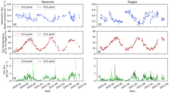
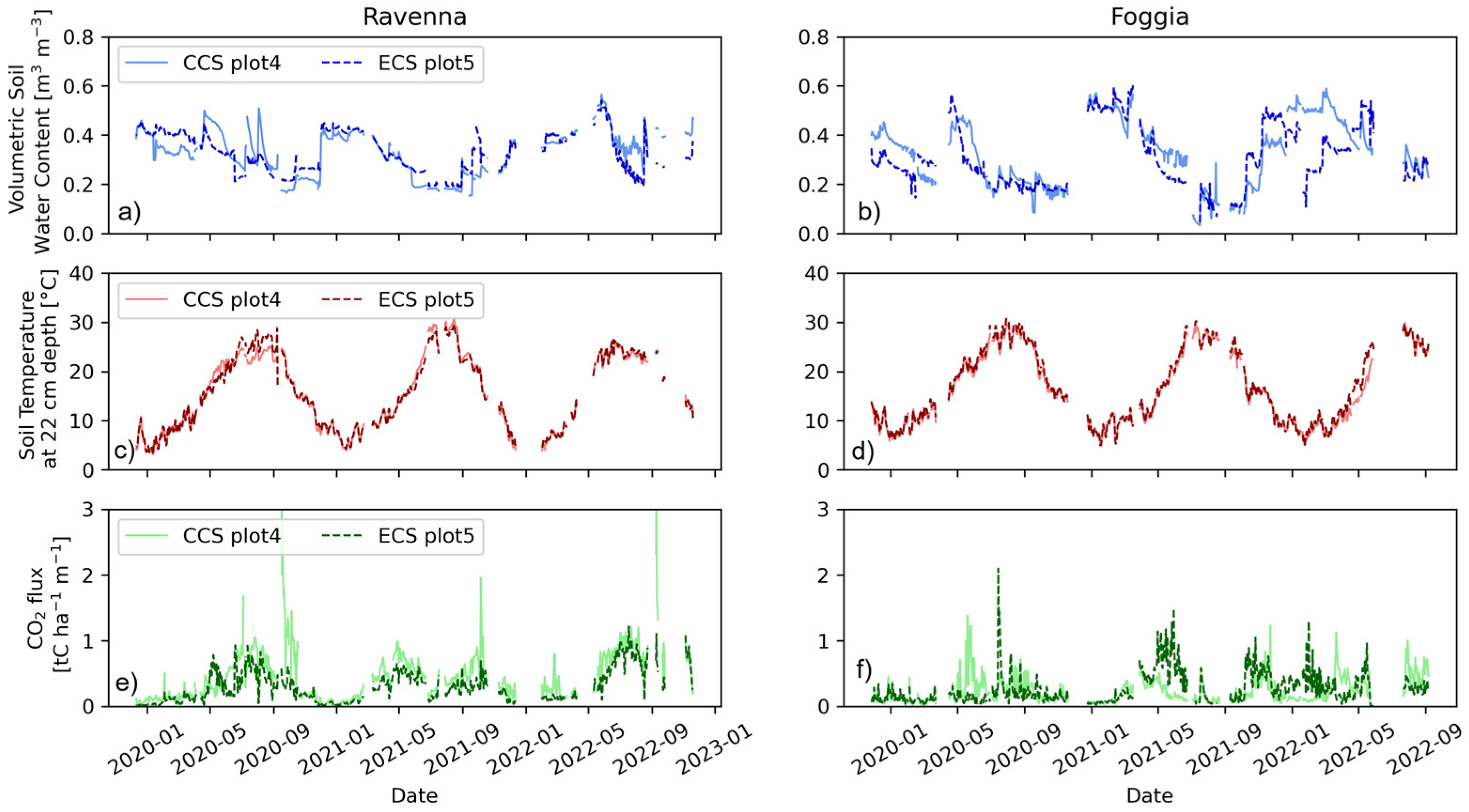
Figure 3 shows the time series measurements taken in the field. The soil water content time series shows small differences between plot 4 (CCS) and plot 5 (ECS) in both sites; depending on the type of crop plantation, one plot may show marginally higher or lower soil water content with respect to the other, but, on average, no clear difference is visible: the average soil water content is 0.33 in both plot 4 and 5 in Ravenna and 0.33 and 0.31 in plot 4 and 5, respectively, in Foggia. During summers the soil water content is always very low in both the Ravenna and Foggia sites, but the lowest values of soil water content are reached in Foggia (minimum values of 0.03 and 0.05 for plot 4 and 5, respectively, compared to 0.15 and 0.18 for plot 4 and 5, respectively, in Ravenna), due to drier weather and different soil properties. The soil temperature does not change between ECS and CCS in general; the temperatures are on average 1 °C higher in Foggia than in Ravenna. The crop dry yield was higher in ECS for durum wheat in both field sites (+ 2% in Ravenna and + 18% in Foggia) and similar between ECS and CCS for other crops such as tomato (+3% in Ravenna); overall, the dry biomass production was higher in ECS due to the presence of cover crops (around 1 t ha⁻¹ yr⁻¹).

Figure 3. Measurements of soil water content (Ravenna (a) and Foggia (b)), soil temperature (Ravenna (c) and Foggia (d)), and soil respiration (Ravenna (e) and Foggia (f)) showing both cropping system plots equipped with gas chambers (plot 4 CCS and plot 5 ECS), for the 3 years of the experiment when CO₂ flux data were available. Soil water content measurements are in volumetric water content (volume of water in the soil sample divided by the total volume of the soil sample, dimensionless).

$R_s$ is generally higher in Ravenna than in Foggia, with average $R_s$ rates of 0.38 and 0.25 tC ha⁻¹ month⁻¹, respectively. In Ravenna, the respiration rates are higher in plot 4 (CCS, 0.45 tC ha⁻¹ month⁻¹) than in plot 5 (ECS, 0.30 tC ha⁻¹ month⁻¹); in Foggia, the respiration rates are higher in plot 5 (ECS, 0.27 tC ha⁻¹ month⁻¹) than in plot 4 (CCS, 0.23 tC ha⁻¹ month⁻¹). As expected, $R_s$ is higher when a crop is growing on the soil and shows peaks, with an exponential decrease after harvest. As widely reported in the literature, $R_s$ increases with an increase in soil temperature (there is a mild correlation with a Pearson coefficient of 0.37, p value > 0.001). $R_s$ also shows a mild inverse correlation with soil water content, with a Pearson coefficient of 0.25 (p value > 0.001). The SOC measurements for all the plots are presented in Section 3.3, analysed together with the RothC20_N simulations.

3.2. Soil Respiration Partitioning

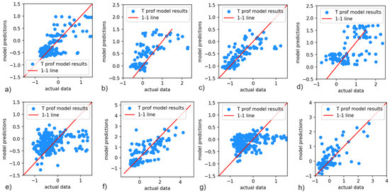
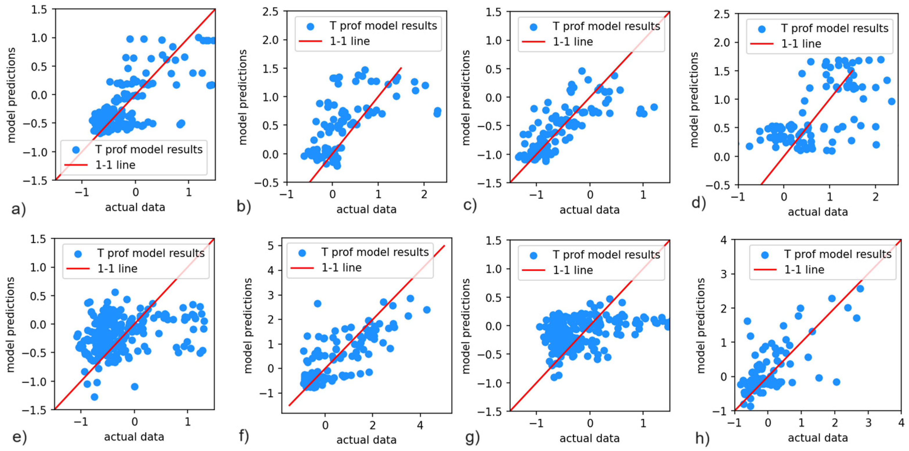
The multiple linear regression modelling for the periods when no crop was present yielded better results in winter (R² of the models = 0.60) than in summer (R² = 0.35) in Ravenna, while the opposite was true in Foggia (R² in summer = 0.51, in winter = 0.12). The residuals (that is, the difference between model estimates and observed values in the no-crop periods) were normally distributed. The estimated $R_a$, i.e., the difference between estimated $R_h$ and measured $R_s$ when the crop was present, showed some degree of correlation with respect to solar radiation, with Pearson correlation coefficients of 0.90 and 0.86 in plot 4 CCS and plot 5 ECS in Ravenna (p values of 0.044 and 0.032, respectively), and 0.63 and 0.41 in plot 4 CCS and plot 5 ECS in Foggia (p values of <0.001 and 0.004, respectively; Figure 4).

Figure 4. Comparison between modelled and observed soil respiration, after normalization, for (a,b) in Ravenna CCS plot 4 in winter and summer, respectively; (c,d) in Ravenna ECS plot 5 in winter and summer, respectively; (e,f) in Foggia CCS plot 4 in winter and summer, respectively; and (g,h) in Foggia ECS plot 5 in winter and summer, respectively.

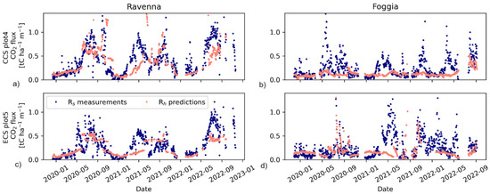
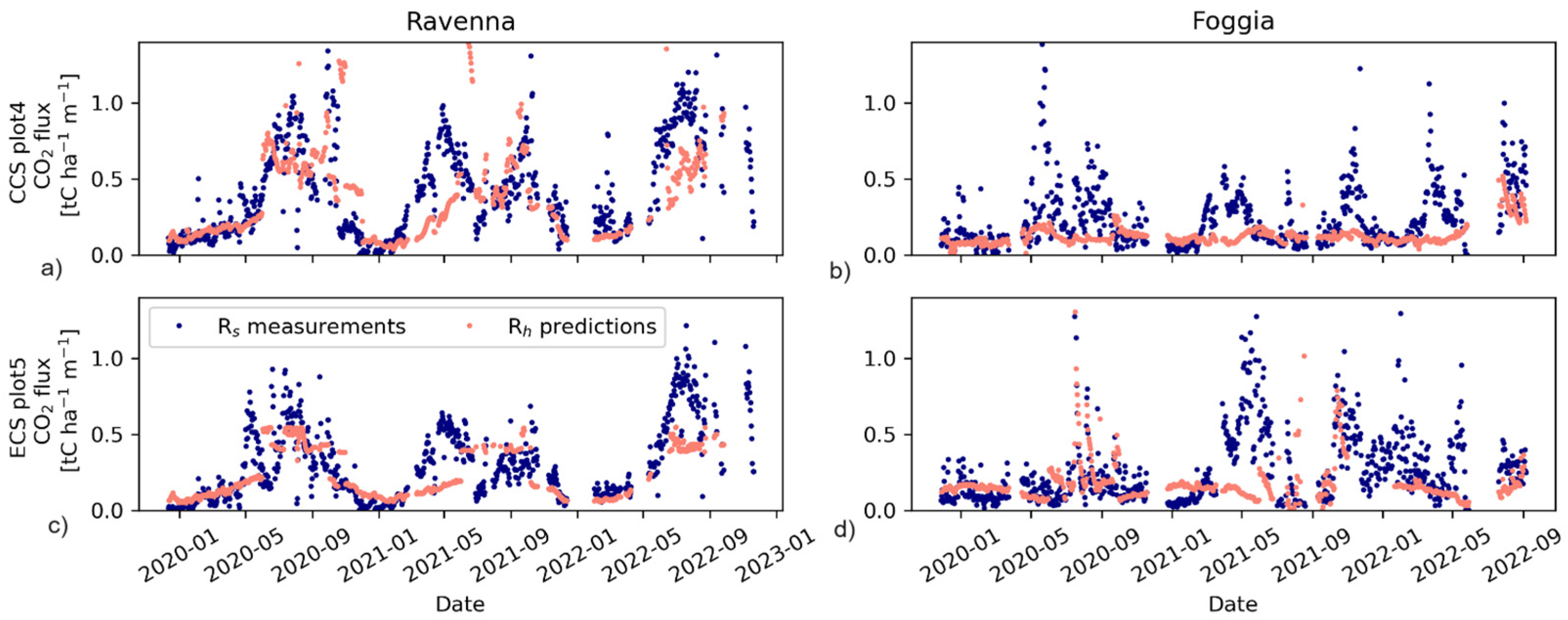
Figure 5 shows the results of $R_s$ partitioning; apart for some periods in which the $R_h$ predictions are larger than the $R_s$ observations, especially in winter 2020 in Foggia and some few days in summer in general, the predictions make sense ($R_s$ larger when crops are growing and standing, $R_h$ large after harvest, then decreasing). In general, the prediction of $R_h$ when crops were present is larger than the $R_s$ observed when $R_s$ was very low in Foggia (winter 2020 in CCS, winters 2019–2020 in ECS) but lower when $R_s$ was large. The average values of the measured $R_s$ are 0.45, 0.23, 0.30, and 0.27 tC ha⁻¹ m⁻¹ for CCS in Ravenna and Foggia and ECS in Ravenna and Foggia, respectively. The corresponding averaged estimates of $R_h$ are 0.45, 0.13, 0.23, and 0.18 tC ha⁻¹ m⁻¹.

Figure 5. $R_s$ measurements and $R_h$ predicted by partitioning, in: (a) Ravenna, plot 4 CCS; (b) Foggia, plot 4 CCS; (c) Ravenna, plot 5 ECS; (d) Foggia, plot 5 ECS; for the 3 years of the experiment when CO₂ flux data were available.

3.3. RothC20_N Simulations

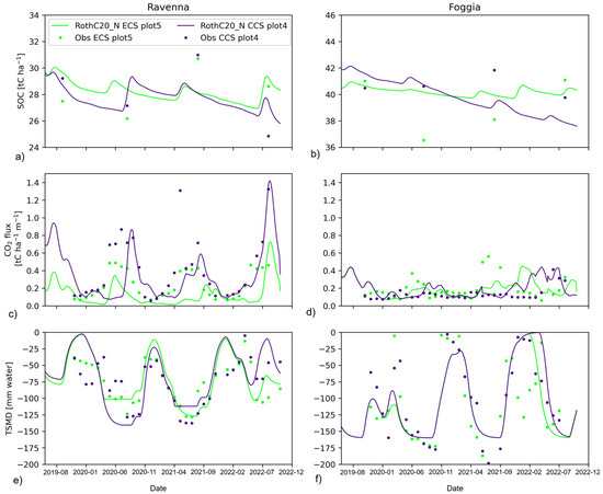
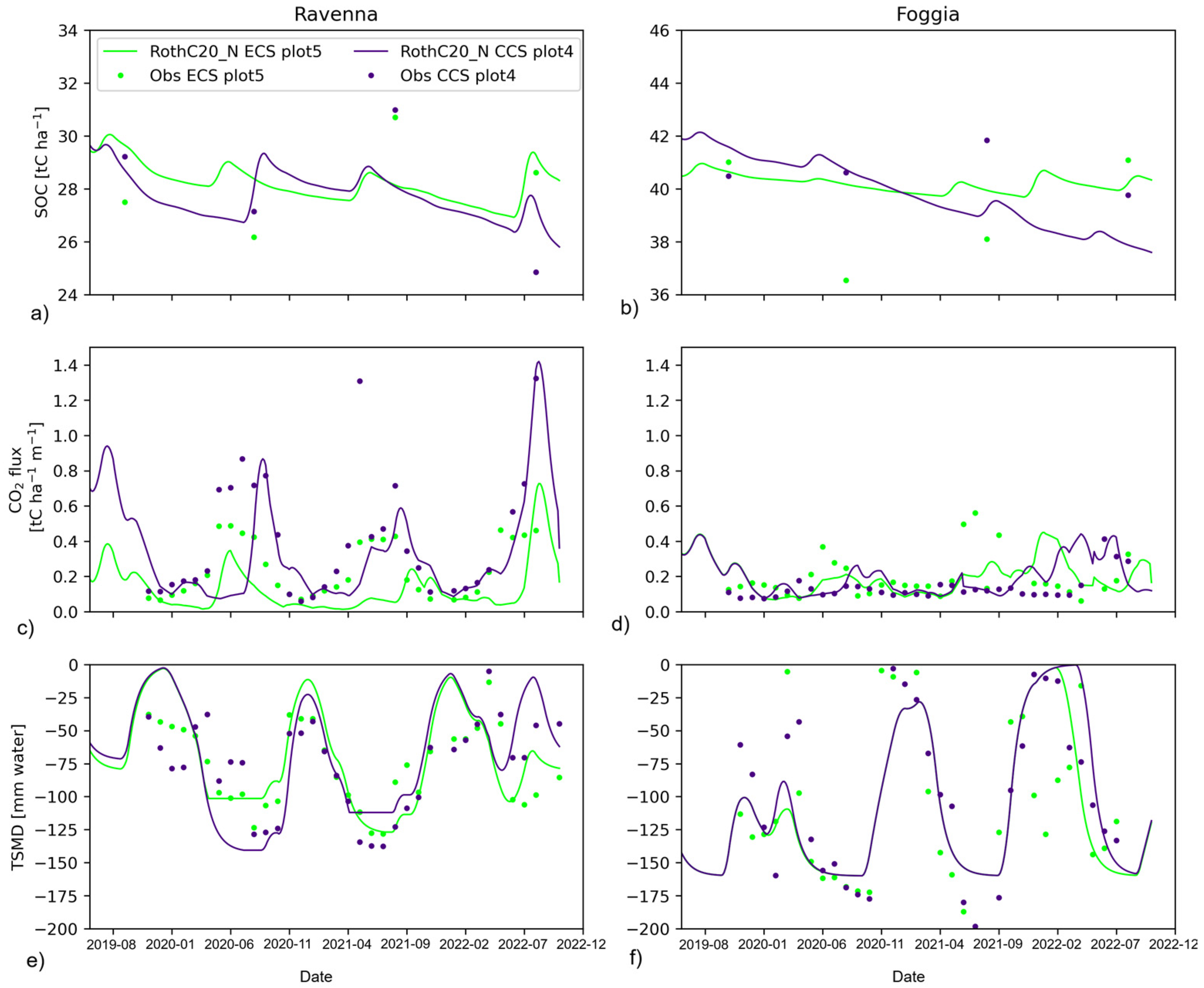
Figure 6 shows the results of the multi-objective calibration. The estimates of the soil water balance parameters from pedotransfer functions as in [36] yielded very good results for RothC20_N (Figure 6e,f, averaged results in Table 1): the very low values reached during summer are well represented, just like the field capacity values during winter. The normalized RMSE values of the model estimates were 0.45 and 0.31 for soil water content, 0.89 and 0.73 for $R_h$, and 0.08 and 0.05 for SOC in plot 4 and plot 5, respectively. The calibration of K_hum, K_rpm, K_bio, and K_dpm were deemed site-specific, that is, the parameters were fitted using data from both treatment (ECS and CCS) for Ravenna. However, the calibration resulted in values very similar to the original ones (5% difference); more specifically, the calibration had only effect on K_hum (0.019 instead of 0.02 yr⁻¹, for both plot 4 and plot 5, since the calibration was conducted simultaneously on both plots). The results show an average Nash–Sutcliff efficiency of 0.3 for the estimated $R_h$; it is possible to see that not all peaks (sudden surges in $R_h$) were well simulated (especially in months 30 and 42 in Ravenna and Foggia), but the average behaviour and the average fluxes matched. The calibrated RothC20_N simulations could model the general SOC trends in the data.

Figure 6. SOC (Ravenna (a) and Foggia (b)), CO₂ flux (Ravenna (c) and Foggia (d)), and TSMD (Ravenna (e) and Foggia (f)) measured and modelled using RothC20_N in the two plots where the gas chamber measures were available (plot 4 CCS and plot 5 ECS) in both field sites (Ravenna and Foggia), after calibrating the RothC20_N models, for the 3 years of the experiment when CO₂ flux data were available.

Table 1. Averages for the data shown in Figure 6, for the period indicated in the figure (October 2019 to October 2022).

		Ravenna		Foggia
		CCS	ECS	CCS	ECS
SOC	tC ha−1	28.05 (27.54)	28.25 (28.02)	40.97 (39.53)	40.40 (40.12)
CO2 flux	tC ha−1 m−1	0.34 (0.30)	0.12 (0.12)	0.16 (0.12)	0.16 (0.12)
TSMD	mm water	−76.59 (−70.11)	−76.73 (70.56)	−98.64 (−102.19)	−109.36 (−109.41)

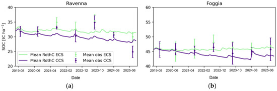
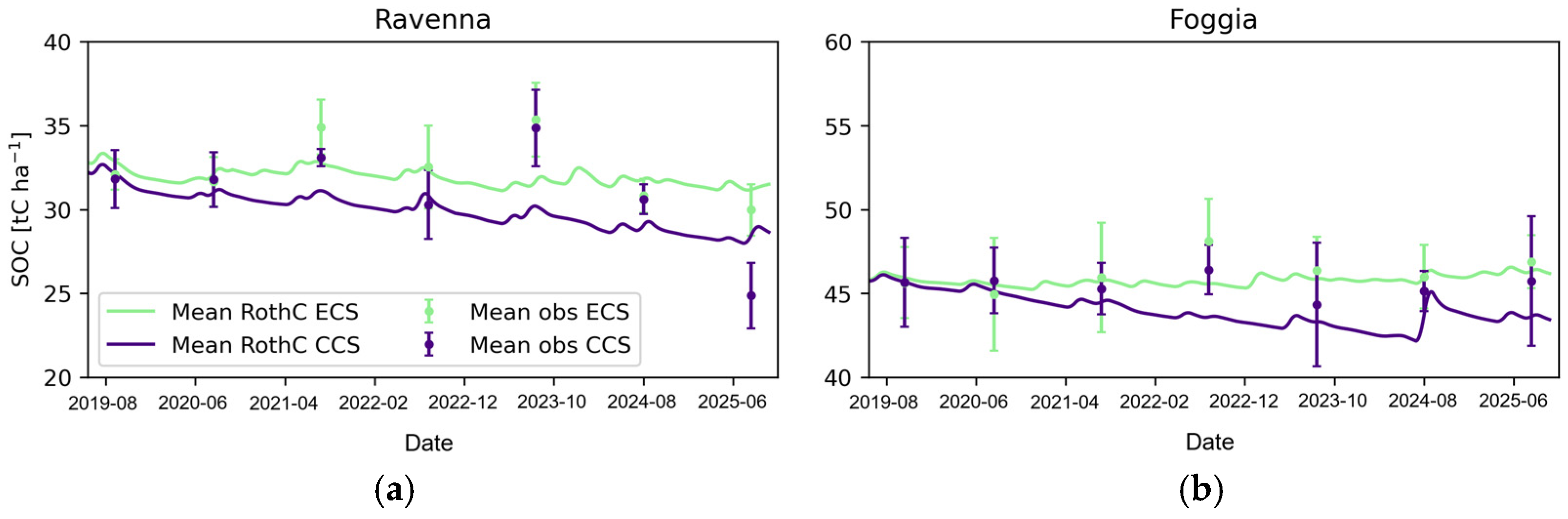
The SOC data were available for all plots; the average values are shown in Figure 7: SOC increased more in ECS than in CCS in both Ravenna and Foggia, but the difference is larger in Ravenna than in Foggia. The SOC trends, however, are characterized by large variability among plots (see error bars in Figure 7), and all trends have R² < 0.1; thus, they do not appear statistically significant, which was expected, since the minimum amount of time to detect a significant trend in SOC has been estimated to be between 5 [17] and 10 years [68]. The carbon input measured on the field, and used as input in the RothC20_N simulations, was as follows: in Ravenna, 11.01 tC ha⁻¹ for CCS and 9.06 tC ha⁻¹ for ECS, of which 1.26 tC ha⁻¹ was due to the incorporation of cover crops in the soil; in Foggia, 6.40 tC ha⁻¹ for CCS and 5.65 tC ha⁻¹ for ECS, of which 1.28 tC ha⁻¹ was due to cover crops.

Figure 7. SOC measured in the field and modelled using RothC20_N, averaged on plots 1, 3, 5, and 7 (ECS) and plots 2, 4, 6, and 8 (CCS) in the (a) Ravenna and (b) Foggia field sites, for the whole 8 years of the experiment.

Figure 7 shows the averaged results for the simulations for all plots, averaged by cropping system (ECS and CCS), in the two field sites; the averaged simulations for Ravenna followed very well the general trend observed in the measurements, with larger SOC values in ECS than in CCS. In Ravenna, the averaged SOC trends estimated by RothC20_N show a stable SOC in ECS and a decrease in CCS; this is also visible in the data (but the observed trend is not statistically significant, with R² values < 0.1). The average normalized RMSE values for the Ravenna site were 0.10 and 0.06 for CCS and ECS respectively, with bias (estimated by the relative error E) not statistically significant.

In Foggia, the simulations show a similar behaviour, with stable SOC in ECS and SOC decrease in CCS, with ECS having increasingly more SOC than CCS. However, the averaged observations show that the trends of ECS and CCS are indistinguishable. In general, in Foggia, the calibrated RothC20_N slightly underestimated SOC in the CCS cropping system. The average normalized RMSE values for the Foggia site were 0.08 and 0.03 for CCS and ECS respectively, with bias (estimated by the relative error E) not statistically significant.

4. Discussion

4.1. Analysis of the Results

Notwithstanding the difference in soil properties and climatic conditions of the two field sites, the differences in the soil conditions that affected SOC pools (that is, soil temperature and soil water content) were very small. The main, even if small, difference was in the soil water content (Figure 3a,b) that was drier in Foggia than in Ravenna, due to the irrigation procedure in Ravenna which increased soil water content whenever reaching wilting point when a crop was present. All these differences in the soil water regime were simulated properly by RothC20_N. $R_s$ appears to be smaller in Foggia than in Ravenna (Figure 3e,f), probably due to the difference in carbon input between the two sites, since this difference was captured by RothC20_N as well (Figure 6c,d). The mild $R_s$ inverse correlation with soil water content can be interpreted by considering what happens in the soil during crop growth: the increase in root respiration happens in conjunction with use of water by the growing crop.

The $R_h$ values estimated with the partitioning method had a relatively high normalized RMSE, but the Nash–Sutcliff efficiency was on average 0.3 (0 means that the model is not better than a simple average, 1 means perfect match between estimates and observations), which shows that the calibrated RothC20_N could model the $R_h$ time series satisfactorily. In fact, the resulting $R_h$ values are very similar to those predicted independently by the RothC20_N simulations even before calibration, giving credibility to both methods. RothC (and RothC20_N) operates at monthly time scales, assuming that the degraded SOC results in CO₂ immediately ejected to the atmosphere, considering the whole upper soil as a bulk model. This level of detail is enough to estimate only average $R_h$ values (see, for example, the $R_h$ estimates in Dondini et al. [54], who employed the ECOSSE model, which uses the same principle as RothC for SOC degradation). The measured peaks in CO₂ outflow are especially dependent on daily or hourly processes, taking place often at specific depths in the soil; Herbst et al. [69] demonstrated that, when RothC SOC degradation calculations are integrated to one-dimensional water, heat, and CO₂ flux models with sub-daily time steps, the estimated $R_h$ resembles more closely the measured ones, being able to predict the emission peaks. In the context of the present study, however, the use of a complex, one-dimensional soil water with coupled water, heat, and gas flow would put an unacceptable burden on the DSS simulations, requiring also a complete rewrite of the DSS, which works on a bulk soil model. Moreover, the focus of this study was the estimate of general SOC trends, not of time series of $R_h$.

The calibration of the RothC20_N model resulted in very good simulations of the soil water regime observed in plots 4 and 5 for both sites, especially for the summer droughts. The calibration could fit satisfactorily both SOC trends without changing appreciably the calibrated parameters, with only 5% change in the initial value of K_hum. In general, the multi-objective calibration method used has great potential, but in our case the estimates from RothC20_N were already close to their calibrated value, so that the calibration had only a very small effect on the model parameters. The analysis of the normalized RMSE for the SOC estimates show low errors overall, with small and non-statistically significant bias. In general, the normalized RMSE is a little higher in the CCS than in the ECS, both in the calibration (0.08 and 0.05 for CCS and ECS, respectively) and in the validation (0.09 and 0.04 for CCS and ECS, respectively); however, the difference is very small.

The comparison between the two field managements, ECS and CCS, showed that ECS decreased CO₂ emissions from the field. In general, we could see less CO₂ emissions (−33%), less use of fertilizers, less use of water, same or better crop yields, and an increase in SOC from measurements, with a small increase trend in SOC (but with small statistical significance). Thus, the ECS method generates more or equal agricultural output with respect to CCS, while decreasing the amount of input. The decrease in fertilizer application and irrigation is likely to result in a reduction in indirect CO₂ emissions as well, i.e., emissions produced before field activity, but this should be evaluated properly in a life cycle analysis (LCA) study. If carbon accounting methods would be put in place, or in the case there was a standardized methodology to reward soil carbon sequestration alongside emission reductions, ECS would be even more interesting as a practice for the farmers, due to both the reduced emissions and increased carbon stored in the soil. Moreover, [70], using LUCAS data from across the EU, showed that properly managed agriculture may result in larger soil microbial diversity with respect to other land uses, even natural grasslands.

4.2. Study Limitations

Some mismatch is evident in the peaks of $R_h$ partitioned and simulated by RothC20_N, especially in August–September 2020 and May–June 2021 (Simulation months 30–31 and 41–42, Figure 6c,d). In Ravenna, ECS simulation shows similar peaks as $R_h$ partitioned, but of lower intensity, while CCS seems to miss the peaks by a few months; in Foggia, ECS partitioned $R_h$ shows peaks that are completely absent from the $R_h$ simulated. Unfortunately, as discussed above, the RothC model, due to its temporal and special scales, is not suited to predict specific peaks in soil respiration, unless integrated into a more detailed soil heat and flux model [69]. However, the level of agreement between the estimated and measured $R_h$ in this study is very good when compared to similar studies using a large $R_h$ dataset [54] or multi-objective calibration methods [38]. Soil enzymatic activity measurements could have helped to better understand $R_h$ dynamics (especially the peaks); unfortunately, such measurements were not collected in this study.

A possible explanation for the slight underestimation of $R_h$ in the Foggia site could be the formation of soil cracks, typical for vertisols, observed in the field. If the cracks are deep enough (in this case, around 30 cm), they may affect the direction of the outflow of CO₂ from the soil, decreasing the reliability of the gas chamber measurements. The formation of deep cracks has been observed only during prolonged droughts; in this study, this corresponds to summer-fall 2020 and summer 2021. Fortunately, low, stable $R_s$ values were recorded in said periods; therefore, the effects on the statistical analysis conducted on $R_s$ (described in Section 2.4) were very small. The formation of soil cracks can substantially influence the rate of outflow of CO₂ from the soil, as described in the literature [71], this could be taken into account by measuring properly the effects of soil cracks using validated methodologies [72,73] and modifying RothC, including some simplified representation of the process.

Another limitation is that RothC20_N is based on a well-established and widely used model (RothC), but the scientific consensus is that such models are not able to properly model the processes regulating the carbon dynamics in the field, and thus they are not robust against changes in the soil conditions (e.g., due to climate change or due to changes in soil management). Even though this problem has been recognized for more than a decade [74], there are still no reliable and applicable successors to RothC- and Century-like models.

5. Conclusions

This study shows that:

• The DSS informed cropping system (ECS) resulted in higher SOC concentrations with respect to the conventional cropping system (CCS), based on 8 years of SOC data.
• The ECS cropping system resulted in 33% less CO₂ emissions from the soil, while increasing the agricultural yields with respect to CCS.
• RothC20_N, after multi-objective calibration, was able to properly fit the soil water content conditions, the heterotrophic component of soil respiration, and the SOC observed in the calibration plots in the Ravenna site.
• The calibrated RohC20_N was also able to estimate the SOC in the ECS and CCS validation plots in the Foggia site.

This study shows that the use of field sensors communicating with agricultural DSS models can result in agricultural practices that are environmentally sustainable. In this study, we were able to show decreases in the carbon emitted by the soil and a reduction in fertilizers and water used in the field, without any negative impact on the yield (or, in some cases, even increasing it). The sequestration of carbon from the atmosphere is paramount to balance anthropic emissions and help reach carbon neutrality; in the future, a carbon market or some type of carbon accounting will probably increase the desirability of carbon farming in agriculture.

RothC20_N by Farina et al. [36] for Mediterranean conditions performed very well in its prediction of soil water content in the experimental fields, since it was able to properly reproduce the soil conditions during long periods without precipitations. This is particularly relevant in a changing climate, where more intense precipitation events and longer dry spells are expected over most of the European continent. RothC20_N proved to be a candidate carbon dynamics model for inclusion in a DSS aimed at helping farmers and decision-makers to consider soil carbon sequestration while maintaining high levels of agricultural productivity.

However, to perform the integration between the SOC model and the DSS, the SOC model must be modified to automatically include all inputs and other soil modelling modules in the DSS, more specifically, the agricultural practices, the DSS representation of crop properties and daily growth, the irrigation management and the soil water budget module (with leaching estimates), and other GHG emissions from farming activities. These modifications and integration strategies will be discussed in a companion article “A tool for Carbon Farming Combining Soil Organic Carbon Modelling and Agricultural Decision Support Systems: Part 2”.

References

- de Brogniez, D.; Ballabio, C.; Stevens, A.; Jones, R.J.A.; Montanarella, L.; van Wesemael, B. A Map of the Topsoil Organic Carbon Content of Europe Generated by a Generalized Additive Model. Eur. J. Soil Sci. 2015, 66, 121–134. [Google Scholar] [CrossRef] [Scilit]
- Dimassi, B.; Mary, B.; Wylleman, R.; Labreuche, J.; Couture, D.; Piraux, F.; Cohan, J.-P. Long-Term Effect of Contrasted Tillage and Crop Management on Soil Carbon Dynamics during 41 Years. Agric. Ecosyst. Environ. 2014, 188, 134–146. [Google Scholar] [CrossRef] [Scilit]
- Committee on the Environment, Public Health and Food Safety. DRAFT REPORT on the Proposal for a Regulation of the European Parliament and of the Council Establishing a Union Certification Framework for Carbon Removals; European Parliament: Strasbourg, France, 2022. [Google Scholar]
- Li, M.; Peng, J.; Lu, Z.; Zhu, P. Research Progress on Carbon Sources and Sinks of Farmland Ecosystems. Resour. Environ. Sustain. 2023, 11, 100099. [Google Scholar] [CrossRef] [Scilit]
- Abbas, F.; Hammad, H.M.; Ishaq, W.; Farooque, A.A.; Bakhat, H.F.; Zia, Z.; Fahad, S.; Farhad, W.; Cerdà, A. A Review of Soil Carbon Dynamics Resulting from Agricultural Practices. J. Environ. Manag. 2020, 268, 110319. [Google Scholar] [CrossRef] [Scilit] [PubMed]
- Schreefel, L.; Schulte, R.P.O.; de Boer, I.J.M.; Schrijver, A.P.; van Zanten, H.H.E. Regenerative Agriculture—The Soil Is the Base. Glob. Food Secur. 2020, 26, 100404. [Google Scholar] [CrossRef] [Scilit]
- Ventura, F.; Poggi, G.M.; Vignudelli, M.; Bosi, S.; Negri, L.; Fakaros, A.; Dinelli, G. An Assessment of Proso Millet as an Alternative Summer Cereal Crop in the Mediterranean Basin. Agronomy 2022, 12, 609. [Google Scholar] [CrossRef] [Scilit]
- Ipcc. Global Warming of 1.5 °C: IPCC Special Report on Impacts of Global Warming of 1.5 °C Above Pre-Industrial Levels in Context of Strengthening Response to Climate Change, Sustainable Development, and Efforts to Eradicate Poverty, 1st ed.; Cambridge University Press: Cambridge, UK, 2022; ISBN 978-1-00-915794-0. [Google Scholar]
- Chambers, A.; Lal, R.; Paustian, K. Soil Carbon Sequestration Potential of US Croplands and Grasslands: Implementing the 4 per Thousand Initiative. J. Soil Water Conserv. 2016, 71, 68A–74A. [Google Scholar] [CrossRef] [Scilit]
- Lehmann, J.; Kleber, M. The Contentious Nature of Soil Organic Matter. Nature 2015, 528, 60–68. [Google Scholar] [CrossRef] [Scilit] [PubMed]
- Lal, R. Soil Carbon Sequestration Impacts on Global Climate Change and Food Security. Science 2004, 304, 1623–1627. [Google Scholar] [CrossRef] [Scilit] [PubMed]
- Zibilske, L.M. Carbon Mineralization. In Methods of Soil Analysis; John Wiley & Sons, Ltd.: Hoboken, NJ, USA, 1994; pp. 835–863. ISBN 978-0-89118-865-0. [Google Scholar]
- Kuzyakov, Y. Sources of CO2 Efflux from Soil and Review of Partitioning Methods. Soil Biol. Biochem. 2006, 38, 425–448. [Google Scholar] [CrossRef] [Scilit]
- Liu, C.; Lu, M.; Cui, J.; Li, B.; Fang, C. Effects of Straw Carbon Input on Carbon Dynamics in Agricultural Soils: A Meta-Analysis. Glob. Change Biol. 2014, 20, 1366–1381. [Google Scholar] [CrossRef] [Scilit] [PubMed]
- Wang, W.; Akhtar, K.; Ren, G.; Yang, G.; Feng, Y.; Yuan, L. Impact of Straw Management on Seasonal Soil Carbon Dioxide Emissions, Soil Water Content, and Temperature in a Semi-Arid Region of China. Sci. Total Environ. 2019, 652, 471–482. [Google Scholar] [CrossRef] [Scilit] [PubMed]
- Sánchez-Cañete, E.P.; Scott, R.L.; van Haren, J.; Barron-Gafford, G.A. Improving the Accuracy of the Gradient Method for Determining Soil Carbon Dioxide Efflux. J. Geophys. Res. Biogeosci. 2017, 122, 50–64. [Google Scholar] [CrossRef] [Scilit]
- Paustian, K.; Collier, S.; Baldock, J.; Burgess, R.; Creque, J.; DeLonge, M.; Dungait, J.; Ellert, B.; Frank, S.; Goddard, T.; et al. Quantifying Carbon for Agricultural Soil Management: From the Current Status toward a Global Soil Information System. Carbon Manag. 2019, 10, 567–587. [Google Scholar] [CrossRef] [Scilit]
- T.m., K.K.; Pal, S.; Chand, P.; Kandpal, A. Carbon Sequestration Potential of Sustainable Agricultural Practices to Mitigate Climate Change in Indian Agriculture: A Meta-Analysis. Sustain. Prod. Consum. 2023, 35, 697–708. [Google Scholar] [CrossRef] [Scilit]
- Quintarelli, V.; Radicetti, E.; Allevato, E.; Stazi, S.R.; Haider, G.; Abideen, Z.; Bibi, S.; Jamal, A.; Mancinelli, R. Cover Crops for Sustainable Cropping Systems: A Review. Agriculture 2022, 12, 2076. [Google Scholar] [CrossRef] [Scilit]
- Meng, X.; Meng, F.; Chen, P.; Hou, D.; Zheng, E.; Xu, T. A Meta-Analysis of Conservation Tillage Management Effects on Soil Organic Carbon Sequestration and Soil Greenhouse Gas Flux. Sci. Total Environ. 2024, 954, 176315. [Google Scholar] [CrossRef] [Scilit] [PubMed]
- Faehnrich, B.; Kirchhof, G.; Hulugalle, N.; Goebel, B. Carbon Sequestration in Australian Vertisols under Conservation Agriculture—Facts and Public Perception. Int. Soil Water Conserv. Res. 2026, 14, 100557. [Google Scholar] [CrossRef] [Scilit]
- Parihar, C.M.; Parihar, M.D.; Sapkota, T.B.; Nanwal, R.K.; Singh, A.K.; Jat, S.L.; Nayak, H.S.; Mahala, D.M.; Singh, L.K.; Kakraliya, S.K.; et al. Long-Term Impact of Conservation Agriculture and Diversified Maize Rotations on Carbon Pools and Stocks, Mineral Nitrogen Fractions and Nitrous Oxide Fluxes in Inceptisol of India. Sci. Total Environ. 2018, 640–641, 1382–1392. [Google Scholar] [CrossRef] [Scilit] [PubMed]
- Kumar, N.; Nath, C.P.; Hazra, K.K.; Das, K.; Venkatesh, M.S.; Singh, M.K.; Singh, S.S.; Praharaj, C.S.; Singh, N.P. Impact of Zero-till Residue Management and Crop Diversification with Legumes on Soil Aggregation and Carbon Sequestration. Soil Tillage Res. 2019, 189, 158–167. [Google Scholar] [CrossRef] [Scilit]
- Smith, P.; Soussana, J.-F.; Angers, D.; Schipper, L.; Chenu, C.; Rasse, D.P.; Batjes, N.H.; van Egmond, F.; McNeill, S.; Kuhnert, M.; et al. How to Measure, Report and Verify Soil Carbon Change to Realize the Potential of Soil Carbon Sequestration for Atmospheric Greenhouse Gas Removal. Glob. Change Biol. 2020, 26, 219–241. [Google Scholar] [CrossRef] [Scilit] [PubMed]
- Eggleston, H.S.; Buendia, L.; Miwa, K.; Ngara, T.; Tanabe, K. 2006 IPCC Guidelines for National Greenhouse Gas Inventories; IPCC: Geneva, Switzerland, 2006; Volume 4. [Google Scholar]
- Pilvere, I.; Nipers, A.; Krievina, A.; Upite, I.; Kotovs, D. LASAM Model: An Important Tool in the Decision Support System for Policymakers and Farmers. Agriculture 2022, 12, 705. [Google Scholar] [CrossRef] [Scilit]
- Whittaker, C.; McManus, M.; Smith, P. A Comparison of Carbon Accounting Tools for Arable Crops in the United Kingdom. Environ. Model. Softw. 2013, 46, 228–239. [Google Scholar] [CrossRef] [Scilit]
- Paustian, K.; Easter, M.; Brown, K.; Chambers, A.; Eve, M.; Huber, A.; Marx, E.; Layer, M.; Stermer, M.; Sutton, B.; et al. Field- and Farm-Scale Assessment of Soil Greenhouse Gas Mitigation Using COMET-Farm. In Precision Conservation: Geospatial Techniques for Agricultural and Natural Resources Conservation; John Wiley & Sons, Ltd.: Hoboken, NJ, USA, 2017; pp. 341–359. ISBN 978-0-89118-356-3. [Google Scholar]
- Forrester, D.I.; England, J.R.; Paul, K.I.; Roxburgh, S.H. Sensitivity Analysis of the FullCAM Model: Context Dependency and Implications for Model Development to Predict Australia’s Forest Carbon Stocks. Ecol. Model. 2024, 489, 110631. [Google Scholar] [CrossRef] [Scilit]
- Paul, K.I.; Polglase, P.J.; Richards, G.P. Predicted Change in Soil Carbon Following Afforestation or Reforestation, and Analysis of Controlling Factors by Linking a C Accounting Model (CAMFor) to Models of Forest Growth (3PG), Litter Decomposition (GENDEC) and Soil C Turnover (RothC). For. Ecol. Manag. 2003, 177, 485–501. [Google Scholar] [CrossRef] [Scilit]
- Coleman, K.; Jenkinson, D.S. RothC-26.3—A Model for the Turnover of Carbon in Soil. In Proceedings of the Evaluation of Soil Organic Matter Models; Powlson, D.S., Smith, P., Smith, J.U., Eds.; Springer: Berlin/Heidelberg, Germany, 1996; pp. 237–246. [Google Scholar]
- FAO. Soil Organic Carbon Mapping Cookbook, 2nd ed.; FAO: Rome, Italy, 2018; ISBN 978-92-5-130440-2. [Google Scholar]
- Paul, K.I.; Polglase, P.J. Calibration of the RothC Model to Turnover of Soil Carbon under Eucalypts and Pines. Soil Res. 2004, 42, 883–895. [Google Scholar] [CrossRef] [Scilit]
- Stamati, F.E.; Nikolaidis, N.P.; Schnoor, J.L. Modeling Topsoil Carbon Sequestration in Two Contrasting Crop Production to Set-aside Conversions with RothC—Calibration Issues and Uncertainty Analysis. Agric. Ecosyst. Environ. 2013, 165, 190–200. [Google Scholar] [CrossRef] [Scilit]
- Lobe, I.; Bol, R.; Ludwig, B.; Du Preez, C.C.; Amelung, W. Savanna-Derived Organic Matter Remaining in Arable Soils of the South African Highveld Long-Term Mixed Cropping: Evidence from 13C and 15N Natural Abundance. Soil Biol. Biochem. 2005, 37, 1898–1909. [Google Scholar] [CrossRef] [Scilit]
- Farina, R.; Coleman, K.; Whitmore, A.P. Modification of the RothC Model for Simulations of Soil Organic C Dynamics in Dryland Regions. Geoderma 2013, 200–201, 18–30. [Google Scholar] [CrossRef] [Scilit]
- Menichetti, L.; Kätterer, T.; Leifeld, J. Parametrization Consequences of Constraining Soil Organic Matter Models by Total Carbon and Radiocarbon Using Long-Term Field Data. Biogeosciences 2016, 13, 3003–3019. [Google Scholar] [CrossRef] [Scilit]
- Cagnarini, C.; Renella, G.; Mayer, J.; Hirte, J.; Schulin, R.; Costerousse, B.; Della Marta, A.; Orlandini, S.; Menichetti, L. Multi-Objective Calibration of RothC Using Measured Carbon Stocks and Auxiliary Data of a Long-Term Experiment in Switzerland. Eur. J. Soil Sci. 2019, 70, 819–832. [Google Scholar] [CrossRef] [Scilit]
- Pesce, S.; Balugani, E.; De Paz, J.M.; Marazza, D.; Visconti, F. A Modified Version of RothC to Model the Direct and Indirect Effects of Rice Straw Mulching on Soil Carbon Dynamics, Calibrated in Two Valencian Citrus Orchards. Soil Syst. 2024, 8, 12. [Google Scholar] [CrossRef] [Scilit]
- Mondini, C.; Cayuela, M.L.; Sinicco, T.; Fornasier, F.; Galvez, A.; Sánchez-Monedero, M.A. Modification of the RothC Model to Simulate Soil C Mineralization of Exogenous Organic Matter. Biogeosciences 2017, 14, 3253–3274. [Google Scholar] [CrossRef] [Scilit]
- Pulcher, R.; Balugani, E.; Ventura, M.; Greggio, N.; Marazza, D. Inclusion of Biochar in a C Dynamics Model Based on Observations from an 8-Year Field Experiment. SOIL 2022, 8, 199–211. [Google Scholar] [CrossRef] [Scilit]
- Beck, H.E.; Zimmermann, N.E.; McVicar, T.R.; Vergopolan, N.; Berg, A.; Wood, E.F. Present and Future Köppen-Geiger Climate Classification Maps at 1-Km Resolution. Sci. Data 2018, 5, 180214. [Google Scholar] [CrossRef] [Scilit] [PubMed]
- Baglivo, C.; Congedo, P.M.; Malatesta, N.A. Building Envelope Resilience to Climate Change under Italian Energy Policies. J. Clean. Prod. 2023, 411, 137345. [Google Scholar] [CrossRef] [Scilit]
- Cola, G.; Mariani, L.; Salinari, F.; Civardi, S.; Bernizzoni, F.; Gatti, M.; Poni, S. Description and Testing of a Weather-Based Model for Predicting Phenology, Canopy Development and Source–Sink Balance in Vitis vinifera L. Cv. Barbera. Agric. For. Meteorol. 2014, 184, 117–136. [Google Scholar] [CrossRef] [Scilit]
- Rossi, V.; Racca, P.; Giosue’, S.; Pancaldi, D.; Alberti, I. A Simulation Model for the Development of Brown Rust Epidemics in Winter Wheat. Eur. J. Plant Pathol. 1997, 103, 453–465. [Google Scholar] [CrossRef] [Scilit]
- Allen, R.G.; Pereira, L.S.; Raes, D.; Smith, M. Crop evapotranspiration-Guidelines for computing crop water requirements-FAO Irrigation and drainage paper 56. Irrig. Drain 1998, 300, D05109. [Google Scholar]
- Gonzales-Dominguez, E.; Legler, S.E.; Fedele, G.; Caffi, T.; Rossi, V. A Web-Based Decision Support System for the Sustainable Management of Vineyards. In Proceedings of the Abstracts Book of International Congress on Grapevine and Wine Sciences, Logroño, La Rioja, Spain, 7 November 2018; p. 82. [Google Scholar]
- Rossi, V.; Meriggi, P.; Caffi, T.; Giosue’, S.; Bettati, T. A Web-Based Decision Support System for Managing Durum Wheat Crops. In Decision Support Systems, Advances in; Intech: Vukovar, Croatia, 2010; pp. 1–26. [Google Scholar]
- Volpi, I.; Bosco, S.; Guidotti, D.; Mammini, M.; Neri, S.; Virgili, G.; Meriggi, P.; Mantino, A.; Laville, P.; Ragaglini, G. Improving GHG Flux Monitoring in Agricultural Soil through the AGRESTIC Prototype: A Focus on the Assessment of Data Quality. In Proceedings of the 2020 IEEE International Workshop on Metrology for Agriculture and Forestry (MetroAgriFor); IEEE: Piscataway, NJ, USA, 2020; pp. 139–143. [Google Scholar]
- ISO 16634-2:2016; Food Products—Determination of the Total Nitrogen Content by Combustion According to Dumas Principle and Calculation of the Crude Protein Content. International Organization for Standardization: Geneva, Switzerland, 2016.
- Raes, D.; Steduto, P.; Hsiao, T.C.; Fereres, E. AquaCrop—The FAO Crop Model to Simulate Yield Response to Water: II. Main Algorithms and Software Description. Agron. J. 2009, 101, 438–447. [Google Scholar] [CrossRef] [Scilit]
- Steduto, P.; Hsiao, T.C.; Raes, D.; Fereres, E. AquaCrop—The FAO Crop Model to Simulate Yield Response to Water: I. Concepts and Underlying Principles. Agron. J. 2009, 101, 426–437. [Google Scholar] [CrossRef] [Scilit]
- Walkley, A.; Black, I.A. An Examination of the Degtjareff Method for Determining Soil Organic Matter, and a Proposed Modification of the Chromic Acid Titration Method. Soil Sci. 1934, 37, 29–38. [Google Scholar] [CrossRef] [Scilit]
- Dondini, M.; Alberti, G.; Delle Vedove, G.; Ventura, M.; Tonon, G.; Viger, M.; Harris, Z.M.; Jenkins, J.R.; Richards, M.; Pogson, M.; et al. Evaluation of the ECOSSE Model to Predict Heterotrophic Soil Respiration by Direct Measurements. Eur. J. Soil Sci. 2017, 68, 384–393. [Google Scholar] [CrossRef] [Scilit]
- Savage, K.E.; Davidson, E.A.; Abramoff, R.Z.; Finzi, A.C.; Giasson, M.-A. Partitioning Soil Respiration: Quantifying the Artifacts of the Trenching Method. Biogeochemistry 2018, 140, 53–63. [Google Scholar] [CrossRef] [Scilit]
- Kucera, C.L.; Kirkham, D.R. Soil Respiration Studies in Tallgrass Prairie in Missouri. Ecology 1971, 52, 912–915. [Google Scholar] [CrossRef] [Scilit]
- Tomotsune, M.; Yoshitake, S.; Watanabe, S.; Koizumi, H. Separation of Root and Heterotrophic Respiration within Soil Respiration by Trenching, Root Biomass Regression, and Root Excising Methods in a Cool-Temperate Deciduous Forest in Japan. Ecol. Res. 2013, 28, 259–269. [Google Scholar] [CrossRef] [Scilit]
- Fitter, A.H.; Self, G.K.; Brown, T.K.; Bogie, D.S.; Graves, J.D.; Benham, D.; Ineson, P. Root Production and Turnover in an Upland Grassland Subjected to Artificial Soil Warming Respond to Radiation Flux and Nutrients, Not Temperature. Oecologia 1999, 120, 575–581. [Google Scholar] [CrossRef] [Scilit] [PubMed]
- Hill, C.; Du, L.; Johnson, M.; McCullough, B.D. Comparing Programming Languages for Data Analytics: Accuracy of Estimation in Python and R. WIREs Data Min. Knowl. Discov. 2024, 14, e1531. [Google Scholar] [CrossRef] [Scilit]
- Coleman, K.; Jenkinson, D.S. RothC—A Model for the Turnover of Carbon in Soil; Rothamsted Research: Harpenden Herts, UK, 2014. [Google Scholar]
- Skjemstad, J.O.; Spouncer, L.R.; Cowie, B.; Swift, R.S. Calibration of the Rothamsted Organic Carbon Turnover Model (RothC Ver. 26.3), Using Measurable Soil Organic Carbon Pools. Soil Res. 2004, 42, 79. [Google Scholar] [CrossRef] [Scilit]
- Zimmermann, M.; Leifeld, J.; Schmidt, M.W.I.; Smith, P.; Fuhrer, J. Measured Soil Organic Matter Fractions Can Be Related to Pools in the RothC Model. Eur. J. Soil Sci. 2007, 58, 658–667. [Google Scholar] [CrossRef] [Scilit]
- Sánchez-Cañete, E.P.; Kowalski, A.S.; Serrano-Ortiz, P.; Pérez-Priego, O.; Domingo, F. Deep CO2 Soil Inhalation/Exhalation Induced by Synoptic Pressure Changes and Atmospheric Tides in a Carbonated Semiarid Steppe. Biogeosciences 2013, 10, 6591–6600. [Google Scholar] [CrossRef] [Scilit]
- Monteith, J.L. The Development and Extension of Penman’s Evaporation Formula. In Application of Soil Physics; Hillel, D., Ed.; Academic Press: New York, NY, USA, 1980. [Google Scholar]
- Beven, K.; Binley, A. GLUE: 20 Years On. Hydrol. Process. 2014, 28, 5897–5918. [Google Scholar] [CrossRef] [Scilit]
- Liu, X.; Kang, S.; Li, F. Simulation of Artificial Neural Network Model for Trunk Sap Flow of {P}yrus Pyrifolia and Its Comparison with Multiple-Linear Regression. Agric. Water Manag. 2009, 96, 939–945. [Google Scholar] [CrossRef] [Scilit]
- Smith, J.; Smith, P. Environmental Modelling: An Introduction; OUP: Oxford, UK, 2007; ISBN 978-0-19-927206-8. [Google Scholar]
- Stockmann, U.; Padarian, J.; McBratney, A.; Minasny, B.; de Brogniez, D.; Montanarella, L.; Hong, S.Y.; Rawlins, B.G.; Field, D.J. Global Soil Organic Carbon Assessment. Glob. Food Secur. 2015, 6, 9–16. [Google Scholar] [CrossRef] [Scilit]
- Herbst, M.; Hellebrand, H.J.; Bauer, J.; Huisman, J.A.; Šimůnek, J.; Weihermüller, L.; Graf, A.; Vanderborght, J.; Vereecken, H. Multiyear Heterotrophic Soil Respiration: Evaluation of a Coupled CO2 Transport and Carbon Turnover Model. Ecol. Model. 2008, 214, 271–283. [Google Scholar] [CrossRef] [Scilit]
- Labouyrie, M.; Ballabio, C.; Romero, F.; Panagos, P.; Jones, A.; Schmid, M.W.; Mikryukov, V.; Dulya, O.; Tedersoo, L.; Bahram, M.; et al. Patterns in Soil Microbial Diversity across Europe. Nat. Commun. 2023, 14, 3311. [Google Scholar] [CrossRef] [Scilit] [PubMed]
- DeCarlo, K.F.; Caylor, K.K. Effects of Crack Morphology on Soil Carbon Flux Dynamics in a Dryland Vertisol. Geoderma 2020, 375, 114478. [Google Scholar] [CrossRef] [Scilit]
- Patterson, B.M.; Furness, A.J.; Bastow, T.P. Soil Gas Carbon Dioxide Probe: Laboratory Testing and Field Evaluation. Environ. Sci. Processes Impacts 2013, 15, 1062–1069. [Google Scholar] [CrossRef] [Scilit] [PubMed]
- Sun, C.; Tang, C.-S.; Vahedifard, F.; Cheng, Q.; Zhou, A.; Shi, B. Field Monitoring of Soil-Atmospheric Interactions in Cracked Soils: Coupled Thermal and Hydrological Responses to Crack Development. Eng. Geol. 2025, 358, 108436. [Google Scholar] [CrossRef] [Scilit]
- Wieder, W.R.; Hartman, M.D.; Sulman, B.N.; Wang, Y.-P.; Koven, C.D.; Bonan, G.B. Carbon Cycle Confidence and Uncertainty: Exploring Variation among Soil Biogeochemical Models. Glob. Change Biol. 2018, 24, 1563–1579. [Google Scholar] [CrossRef] [Scilit] [PubMed]
Disclaimer/Publisher’s Note: The statements, opinions and data contained in all publications are solely those of the individual author(s) and contributor(s) and not of MDPI and/or the editor(s). MDPI and/or the editor(s) disclaim responsibility for any injury to people or property resulting from any ideas, methods, instructions or products referred to in the content. |
© 2026 by the authors. Licensee MDPI, Basel, Switzerland. This article is an open access article distributed under the terms and conditions of the Creative Commons Attribution (CC BY) license.