Study on Carbon Emissions from Highway Service-Area Buildings in Different Climatic Regions of China

Abstract

Highway service-area buildings are characterized by long operating hours, diverse functional spaces, and considerable energy consumption, resulting in significant life-cycle carbon emissions. This study quantifies life-cycle carbon emissions of the buildings in highway service areas. A life-cycle accounting framework was established, and net emissions were further evaluated by considering the contributions of photovoltaic (PV) electricity and vegetation carbon sinks. Five representative service areas covering hot-summer/cold-winter, severe-cold, cold, temperate, and hot-summer/warm-winter zones were investigated through field surveys and indoor thermal environment measurements to obtain envelope properties, equipment configurations, and operating profiles. Results revealed that life-cycle carbon emissions vary substantially across climatic regions, ranging from 4.31 × 10³ to 3.06 × 10⁴ tCO₂e. The operational stage accounts for the largest share of total emissions, approximately 61–84%. Heating demand dominates operational emissions in severe-cold and cold regions, whereas cooling and lighting loads become increasingly important in warm and temperate climates. The orthogonal analysis reveals significant differences in the sensitivity of design parameters across climatic regions. After implementing climate-adaptive optimization measures, life-cycle carbon emissions are reduced by 40.35–87.94% in four service areas. In the hot-summer/warm-winter region, the combined effects of PV electricity generation and vegetation carbon sinks maintain a net-negative carbon balance. The findings provide evidence for sustainable highway service-area design by linking life-cycle accounting, climate-specific design priorities, and renewable-energy substitution.

1. Introduction

Climate change mitigation requires rapid emissions reductions across multiple sectors [1,2]. The interface between transportation infrastructure and the built environment is receiving growing attention [3]. Highway service areas are a typical node in this interface [4]. Their integrated buildings operate for long hours, serve transient users with large temporal fluctuations, and host mixed functions within one envelope [5]. These features shape a load profile that is not identical to that of conventional urban public buildings [6]. Space conditioning can be important, but lighting and plug loads associated with catering and retail equipment often remain high [7]. As expressway networks expand, the associated building carbon footprint becomes increasingly relevant for low-carbon transport strategies.

Climatic conditions are a first-order driver of energy demand and carbon emissions in service-area buildings [8]. China spans multiple climatic regions with large differences in heating and cooling requirements, humidity conditions, envelope design constraints, and renewable-energy resource endowments [9]. In severe-cold and cold regions, heating demand and heating energy supply structure can dominate operational emissions. In hot-summer regions, cooling and dehumidification can become the main operational drivers. In temperate regions, where heating and cooling loads may be moderate, the contribution of lighting and equipment electricity consumption can increase because long operating hours persist while space-conditioning demand is lower [10]. These climate-driven differences imply that a uniform low-carbon package is unlikely to perform equally well nationwide [11]. Instead, climate-adaptive priorities are required: the dominant emission sources should be identified for each climate zone, and design or retrofit decisions should target those drivers first.

From the methodological standpoint, building carbon assessment has largely converged on life-cycle assessment (LCA) frameworks combined with emission-factor-based accounting [12,13]. Across a wide range of building types, the operational stage is typically reported as the dominant contributor, often accounting for more than half of total life-cycle emissions [14,15]. The embodied emissions from materials and construction commonly fall in the order of tens of percent of the life-cycle total, with the exact split depending on climate, energy structure, service life, and building efficiency level [16]. Studies that normalize results by floor area frequently report life-cycle emission intensities on the order of 10²–10³ kgCO₂e·m⁻² over the building life cycle, and operational carbon intensities commonly in the range of 10–100 kgCO₂e·m⁻²·yr⁻¹ [17,18]. In addition, many analyses reveal that once envelope and HVAC efficiencies reach a certain level, the relative importance of non-HVAC end uses increases [19,20]. The lighting and plug loads are becoming key drivers in buildings with long operating hours or high equipment densities. These quantitative patterns provide useful benchmarks, but they are not automatically transferable to highway service-area buildings because their operating profile, end-use composition, and boundary conditions differ from those of typical urban buildings.

For highway service areas, research and practice have expanded from operational energy saving to energy–carbon co-optimization [21]. Operational studies increasingly move beyond annual total energy to end-use decomposition, attempting to quantify the shares of HVAC, lighting, domestic hot water, and plug loads under different functional layouts and schedules [22]. In parallel, service areas have become common sites for integrated energy demonstrations because they often have usable roof area for PV, clear daytime electricity demand, and a growing need for charging infrastructure [23]. Reported projects indicate that PV deployment can offset a substantial fraction of annual electricity use in suitable climates [24]. The addition of storage and energy management can further improve on-site utilization and peak shaving [25]. Some demonstration programs explicitly target near-zero or net-zero outcomes, where renewable substitution and operational optimization are combined [26]. In some cases, additional measures such as landscaping carbon sinks or resource recycling are included as supplementary offsets [27].

Recent studies have further expanded the research basis for low-carbon buildings and sustainable highway infrastructure. Zhao et al. [28] used building information modeling (BIM) and LCA to quantify whole-life carbon emissions of a public building and compared carbon characteristics among different public building types, confirming the value of LCA for building-level carbon diagnosis. Gao et al. [29] applied LCA to highway construction and showed that carbon emissions from transport infrastructure are strongly affected by material production and construction activities. For highway service areas, Han et al. [30] emphasized that expressway service-area buildings are special public buildings with complex functions, large passenger flows, and high energy-consumption intensity. Yu et al. [31] assessed the photovoltaic potential of Chinese expressway service areas and demonstrated that service areas have considerable renewable-energy substitution potential. However, most existing studies focus on conventional public buildings, road construction, integrated energy utilization, or PV potential. Few studies have quantified the life-cycle carbon emissions of highway service-area buildings across different climatic regions under a unified boundary. The climate-dependent priority of design parameters and carbon reduction measures also remains insufficiently clarified.

Several issues remain when the objective is transferable, climate-adaptive guidance for service-area integrated buildings. A first issue is boundary and data consistency in carbon accounting. Many assessments emphasize operational emissions and treat embodied emissions from materials and construction inconsistently [32]. Differences in assumed service life, maintenance treatment, and activity data sources further reduce comparability. A second issue is the limited availability of cross-climate comparative evidence. Many studies are regional case studies, and their conclusions may not generalize because climatic forcing, energy structures, and renewable-resource conditions differ substantially across China [33]. A third issue is prioritization. Mitigation recommendations are often presented as a list of measures or isolated technology evaluations. In contrast, climate-adaptive decision-making requires quantified evidence on which design parameters dominate emission changes in each climate zone [34].

In response to these challenges, the study develops a unified life-cycle carbon assessment and climate-adaptive prioritization for highway service-area integrated buildings in China. Five representative service-area buildings are selected to cover typical climatic regions. The field investigations are conducted to obtain building geometry, envelope thermal properties, equipment configurations, and operating profiles. Indoor thermal environment measurements are carried out to characterize operational conditions and support the interpretation of energy-use patterns. A life-cycle carbon accounting framework is established for construction, operation, and demolition stages. An orthogonal experimental design is applied to quantify the effects of key parameters and support design and retrofit decisions. Finally, net emissions are further evaluated by considering photovoltaic electricity substitution and vegetation carbon sinks where applicable.

The main contribution of this work is to connect highway service-area carbon accounting with sustainable infrastructure planning. First, it provides a cross-climate comparison of highway service-area buildings using a consistent life-cycle boundary. Second, it identifies climate-specific design priorities through orthogonal analysis instead of relying only on generic mitigation measures. Third, it evaluates PV substitution and vegetation carbon sinks as part of the net carbon balance. These results support sustainable service-area planning, carbon-neutral highway infrastructure, and climate-adaptive retrofit decisions.

2. Experimental Sites and Procedures

2.1. Overview of Service Areas

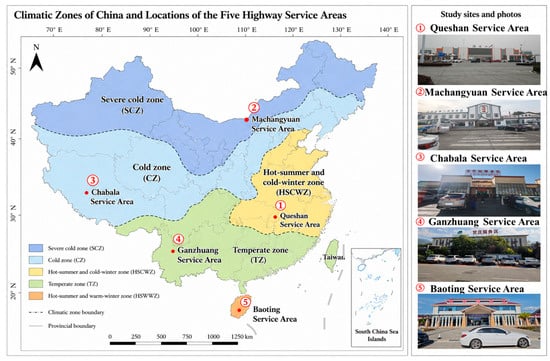
This study adopts a multi-case design to compare carbon-emission characteristics of highway service-area integrated buildings across China’s major climatic regions. The location of the selected services area is shown in Figure 1. The selection criteria were: (i) climatic representativeness; (ii) functional completeness; (iii) availability of design drawings and operational information; and (iv) feasibility of on-site surveys and indoor environmental measurements. Five representative service areas were selected to cover typical building climate zones: Queshan (hot-summer/cold-winter), Machangyuan (severe-cold), Chabala (cold plateau), Ganzhuang (temperate/mild), and Baoting (hot-summer/warm-winter). The selected cases are located along national expressway corridors and include typical service-area functions (lobby/rest hall, catering, retail/supermarket, sanitation, and offices, with partial staff accommodation). The dimensions of the service area of comprehensive buildings are shown in Table 1.

Figure 1. Locations of the selected highway service areas and the corresponding building climate zones.

Table 1. Building and envelope information for the selected service-area buildings.

Location	Floor Height	Area (m2)	Orientation	Form Factor	Exterior Wall System	Roof System
Queshan	H1 = 5.9 m H2 = 4.2 m	3517.32	77° north–northeast	0.23	Masonry wall with insulation layer	Reinforced-concrete roof with insulation layer
Machangyuan	H1 = 4.2 m H2 = 4.2 m	2171.09	45° north–east	0.24	Composite masonry wall with insulation layer	Reinforced-concrete roof with insulation layer
Chabala	H1 = 5.9 m H2 = 3.9 m	1084.3	37° north–west	0.39	Masonry wall with insulation layer	Reinforced-concrete roof with insulation layer
Ganzhuang	H1 = 4.8 m H2 = 3.9 m	3165.45	North	0.29	Masonry wall with insulation layer	Reinforced-concrete roof with insulation layer
Baoting	H1 = 4.8 m H2 = 3.6 m	847.76	40.5° north–east	0.28	Masonry wall with insulation layer	Reinforced-concrete roof with insulation layer

The five cases are selected as representative engineering samples rather than as a statistical sample of all Chinese service areas. Each case corresponds to one major building climate zone and has complete design drawings, operational records, and on-site accessibility. This selection allows controlled comparison under a unified accounting boundary. The limited sample size is acknowledged as a limitation, and the results should be interpreted as climate-zone case evidence rather than national statistical averages.

2.2. Data Collection Procedures

A site-based data collection scheme is implemented to support full life-cycle carbon accounting and analyze operational emissions. The data collection process comprises the following five steps:

• Meteorological information: long-term climate descriptors (temperature and humidity profiles) are compiled for site characterization.
• Building physical attributes: geometry, functional zoning, and envelope properties are obtained from design drawings and verified on site where possible.
• Operational profiles and energy-related inventory: equipment lists, typical operating schedules, and available energy-consumption records are collected through site management interviews and on-site inspection.
• Carbon sink data: Data such as photovoltaic power generation and solar water-heating system efficiency come from the annual reports of operators and real-time monitoring platforms. The vegetation types and carbon sequestration amounts are based on on-site surveys of green areas.
• Data checking and uncertainty control: building drawings, on-site observations, equipment lists, and operator records are cross-checked. Parameters without complete annual records are treated using consistent assumptions across cases and discussed in the uncertainty analysis.

2.3. Indoor Thermal Environment Measurement

Indoor thermal environment measurements are conducted in rest halls during the typical operational periods of the building. Measurement points are arranged based on occupancy distribution and are placed at a standard height of 1.1 m above the ground, corresponding to human activity levels. The JTSOFT-MT2020 multifunctional tester (Beijing Century Jiantong Technology Co., Ltd., Beijing, China) is adopted for field measurement, with measurement accuracies of ±0.5 °C for air temperature, ±3%RH for relative humidity, and ±0.1 m/s for air velocity. The primary monitored parameters include dry-bulb temperature, relative humidity, and air velocity. Data are automatically collected at an interval of 5 min with continuous 24 h monitoring at each measuring point. Meanwhile, the operating status of HVAC systems, real-time occupancy conditions, and outdoor meteorological parameters are synchronously documented.

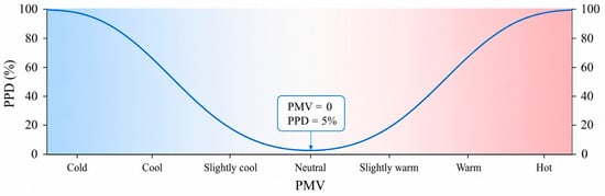
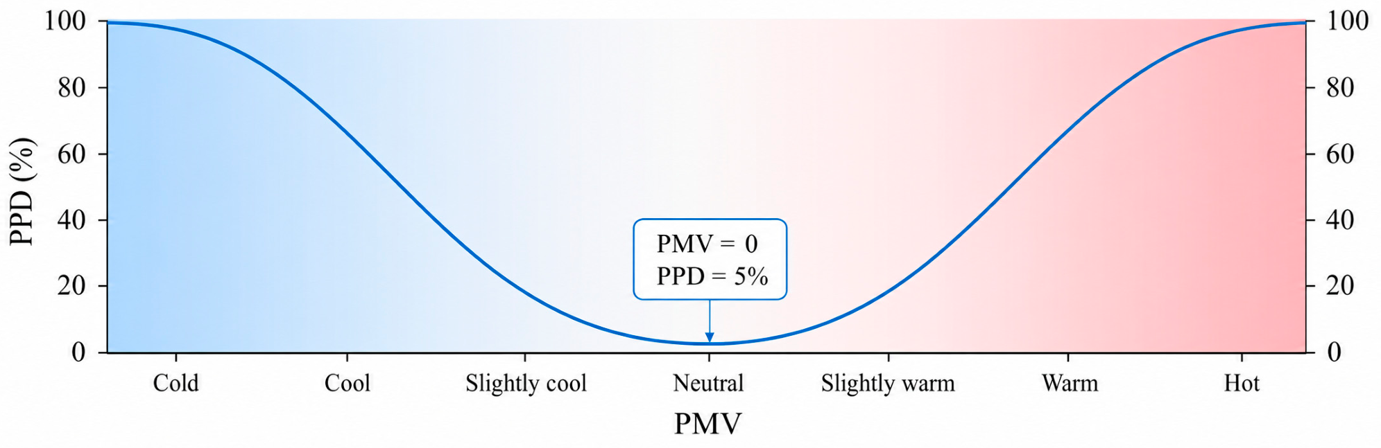
Thermal comfort is quantitatively evaluated using the Predicted Mean Vote (PMV) and Predicted Percentage of Dissatisfied (PPD) framework. ISO 7730 [35] adopts the PMV-PPD model as the criterion for thermal comfort evaluation and recommends a desirable PMV range of −0.5 to +0.5 with a corresponding PPD value no more than 10%. The correlation curve and corresponding numerical values between PMV and PPD are presented in Figure 2 and Table 2, respectively.

Figure 2. Curves corresponding to PMV and PPD.

Table 2. Values corresponding to PMV and PPD.

PMV	PPD	Sense
−3	99.10%	Cold
−2	76.80%	Cool
−1	26.10%	Slightly cool
0	5.00%	Neutral
1	26.10%	Slightly warm
2	76.80%	Warm
3	99.10%	Hot

The PMV-PPD model is adopted to ensure comparability among cases. No questionnaire-based adaptive comfort survey is conducted. The effects of occupant adaptation and transient pedestrian flows are therefore discussed as practical limitations of the present evaluation.

The monitoring campaign represents typical 24 h operational periods. It does not cover all seasonal variations. Therefore, the measured thermal comfort results are used to explain typical operating conditions and emission differences, while long-term seasonal monitoring is identified as a future improvement.

3. Carbon Emissions Accounting Model

This study quantifies the life-cycle carbon emissions of highway service-area integrated buildings using an emission-factor-based approach [36]. The accounting framework covers the construction, operation, and demolition stages, and further evaluates net emissions by considering renewable electricity substitution and vegetation carbon sinks.

3.1. System Boundary

The calculation unit refers to a single integrated building within a highway service area, with a design life of 50 years. Emissions are reported in tCO₂e. Results are also normalized by floor area. Life-cycle totals are reported in kgCO₂e·m⁻². Annualized indicators are reported in tons of carbon dioxide equivalent per year (tCO₂e·m⁻²·yr⁻¹).

The system boundary includes construction, operation, and demolition. The construction stage covers major material production, material transport to the site, and on-site construction. The operation stage covers electricity and fuel use during service. End-use allocation is applied when data allow. The demolition stage covers demolition, waste transport, and waste treatment or disposal.

Recurrent emissions associated with major equipment replacement, interior renovation, and periodic maintenance are not included because consistent long-term maintenance records are unavailable for all five service areas. Minor operation-related energy use is reflected in the operational energy data. This boundary choice is applied consistently across all cases and is further discussed as a source of uncertainty.

3.2. Construction-Stage Emissions

Construction-stage emissions are decomposed into material production, transportation, and on-site construction:

$$C_{con}=C_{mat}+C_{tr}+C_{site}$$

(1)

Material production:

$$C_{mat}=\sum _{\mathrm{m}}{M}_m·E{F}_m$$

(2)

where $M_m$ is the quantity of material m. $E{F}_m$ is the cradle-to-gate emission factor of material m.

Transportation of materials:

$$C_{tr}=\sum _m{M}_m·D_m·{EF}_{tr}$$

(3)

where $D_m$ is the average transport distance for material m. ${EF}_{tr}$ is the transport emission factor.

On-site construction activities:

$$C_{site}=\sum _j{E}_j·{EF}_j$$

(4)

where $E_j$ denotes on-site energy consumption for construction machinery and temporary facilities. Table 3 lists the carbon emission factors for building materials commonly utilized in service-area buildings.

Table 3. The carbon emission factors of construction materials [37,38].

Name	Carbon Emission Factors (kgCO2)	Unit
Cement	735	t
C30 concrete	295	m3
C50 concrete	385	m3
C20 concrete	112	t
Lime	1190	t
Slaked lime	747	t
Concrete bricks	336	m3
Autoclaved fly ash bricks	341	m3
Solid bricks made from sintered fly ash	134	m3
Solid shale bricks	292	m3
Stick to the hollow bricks	250	m3
Solid bricks made from coal gangue	22.8	m3
Ferroalloys for steelmaking	9530	t
Mild steel	2050	t
Hot-rolled carbon steel	2380	t
Aluminum sheets and strips	28,500	t
Extruded polystyrene insulation boards	22.7	m3
Extruded polystyrene board	669	m3
Polystyrene	4620	t

3.3. Operational-Stage Emissions

Operational emissions are calculated from electricity and fuel consumption over the service life:

$$C_{op}=L·\left(C_{el}+C_{fuel}+C_{ref}\right)$$

(5)

where $L$ is the service life in years. $C_{el}$ represents the annual indirect emissions from electricity use. $C_{fuel}$ represents the annual direct emissions from on-site fuel use. $C_{ref}$ represents the annual emissions associated with refrigerant leakage.

Annual electricity-related emissions are calculated as follows:

$$C_{el}={EF}_{grid}·\left(E_{HVAC}+E_{light}+E_{elec}+E_{DHW}+E_{aux}\right)$$

(6)

where ${EF}_{grid}$ is the grid emission factor. $E_{HVAC}$, $E_{light}$, $E_{elec}$, $E_{DHW}$, and $E_{aux}$ are the annual electricity consumption of HVAC, lighting, elevators, domestic hot water, and other equipment, respectively.

Annual fuel-related emissions are calculated as follows:

$$C_{fuel}=\sum _f{EF}_f·Q_f$$

(7)

where $Q_f$ is the annual consumption of fuel f. ${EF}_f$ is its emission factor. Fuels may include liquefied petroleum gas or natural gas for cooking, and diesel for backup power. Several energy-related carbon emission factors are shown in Table 4.

Table 4. Several energy-related carbon emission factors [39,40].

Types	Name	Carbon Emission Factors (tCO2/t)
Solid fuel	Anthracite	94.44
	Bituminous coal	89
	Lignite	98.56
	Coking coal	91.27
	Briquettes	110.88
	Other coking products	100.6
Liquid fuel	Crude oil	72.23
	Fuel	75.82
	Petrol	67.91
	Diesel	72.59
	Kerosene	70.43
	Liquefied petroleum gas	61.81
	Petrochemical feedstock	71.87
	Other oils	71.87
Gaseous fuel	Gas	55.54

3.4. Demolition-Stage Emissions

Demolition-stage emissions are included to complete the life-cycle boundary. They mainly arise from demolition activities, construction-waste transport, and waste treatment. In practice, the total energy use and the recycling rate at the end of life are difficult to determine for service-area buildings because demolition and recovery technologies in the future are uncertain. This study applies an empirical estimation method. Case statistics from building life-cycle assessments indicate that demolition-related emissions, including waste transport and treatment, typically account for about 5% to 15% of the construction-stage emissions [41]. This empirical range is also consistent with the whole-life carbon accounting boundary defined in GB/T 51366-2019 [21,42]. The demolition-stage emissions are calculated as follows:

$$C_{dem}=\alpha ·C_{con}$$

(8)

where $C_{dem}$ represents the demolition-stage carbon emissions. $C_{con}$ represents the construction-stage carbon emissions. $\alpha$ is the demolition-to-construction ratio. In this study, $\alpha$ is set to 0.10.

A simple sensitivity check is added for the empirical demolition coefficient. When alpha varies from 0.05 to 0.15, the resulting change in total life-cycle emissions is approximately 0.8–1.9% for the five cases. Thus, the fixed value of 0.10 has a limited influence on the cross-case ranking, although more detailed end-of-life inventories would improve future assessments.

3.5. Photovoltaic and Vegetation Carbon Sinks

Net life-cycle emissions are evaluated by introducing two offset terms within the service-area boundary [43]. One term represents avoided grid emissions from on-site photovoltaic electricity. The other term represents carbon sequestration by on-site vegetation.

Photovoltaic substitution is quantified by converting PV electricity to avoided grid emissions. Avoided emissions are calculated as

$$C_{PV}=\sum _{y=1}^L{E}_{PV,y}·{EF}_{grid,y}{C}_{con}=C_{mat}+C_{tr}+C_{site}$$

(9)

where $E_{PV,y}$ is PV electricity in year y. ${EF}_{grid,y}$ is the grid emission factor. Metered PV generation is used when available. The PV electricity is estimated from installed capacity and local solar resources using a consistent performance assumption [44].

For the base calculation, PV generation and the grid emission factor are treated as constant over the 50-year service life. This assumption represents a current-grid scenario. If future grid decarbonization is considered, the avoided emissions from PV electricity would decrease. Module degradation, inverter replacement, and storage losses are not included because site-specific long-term operation data are unavailable.

Vegetation carbon sinks are quantified using an area-based sequestration approach. Annual sequestration is calculated as follows:

$$S_v=\sum _v{A}_v{\gamma }_v$$

(10)

where $A_v$ is the area of vegetation typ. ${\gamma }_v$ is the sequestration coefficient. When vegetation types are not available, a site-averaged coefficient is applied to the total green area. The life-cycle sink is aggregated as follows:

$$C_{sink}=\sum _{y=1}^L{S}_y$$

(11)

Annual sequestration is assumed constant over the service life to maintain cross-case consistency and to avoid introducing uncertain growth dynamics [27,45].

This assumption simplifies the growth dynamics of vegetation. In practice, sequestration capacity varies with species, age, irrigation, pruning, and local maintenance. The calculated vegetation sink should therefore be interpreted as a planning-level offset rather than a dynamic ecological carbon model.

4. Results

4.1. Indoor Hydrothermal Measurements and Thermal Comfort

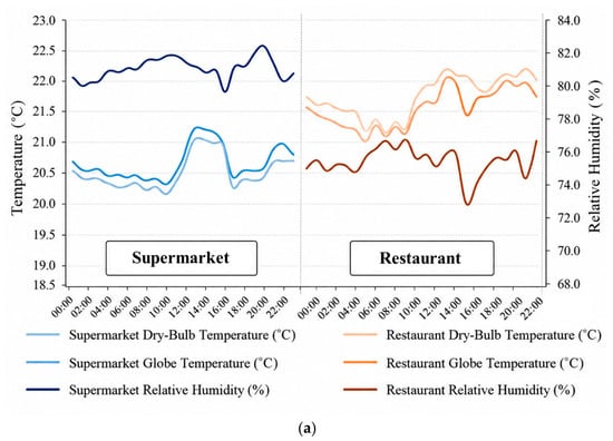
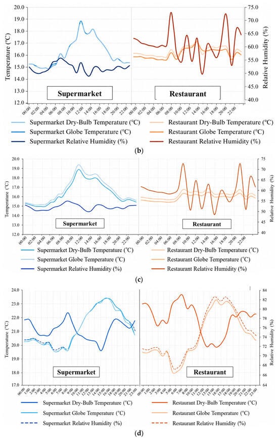
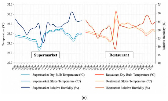
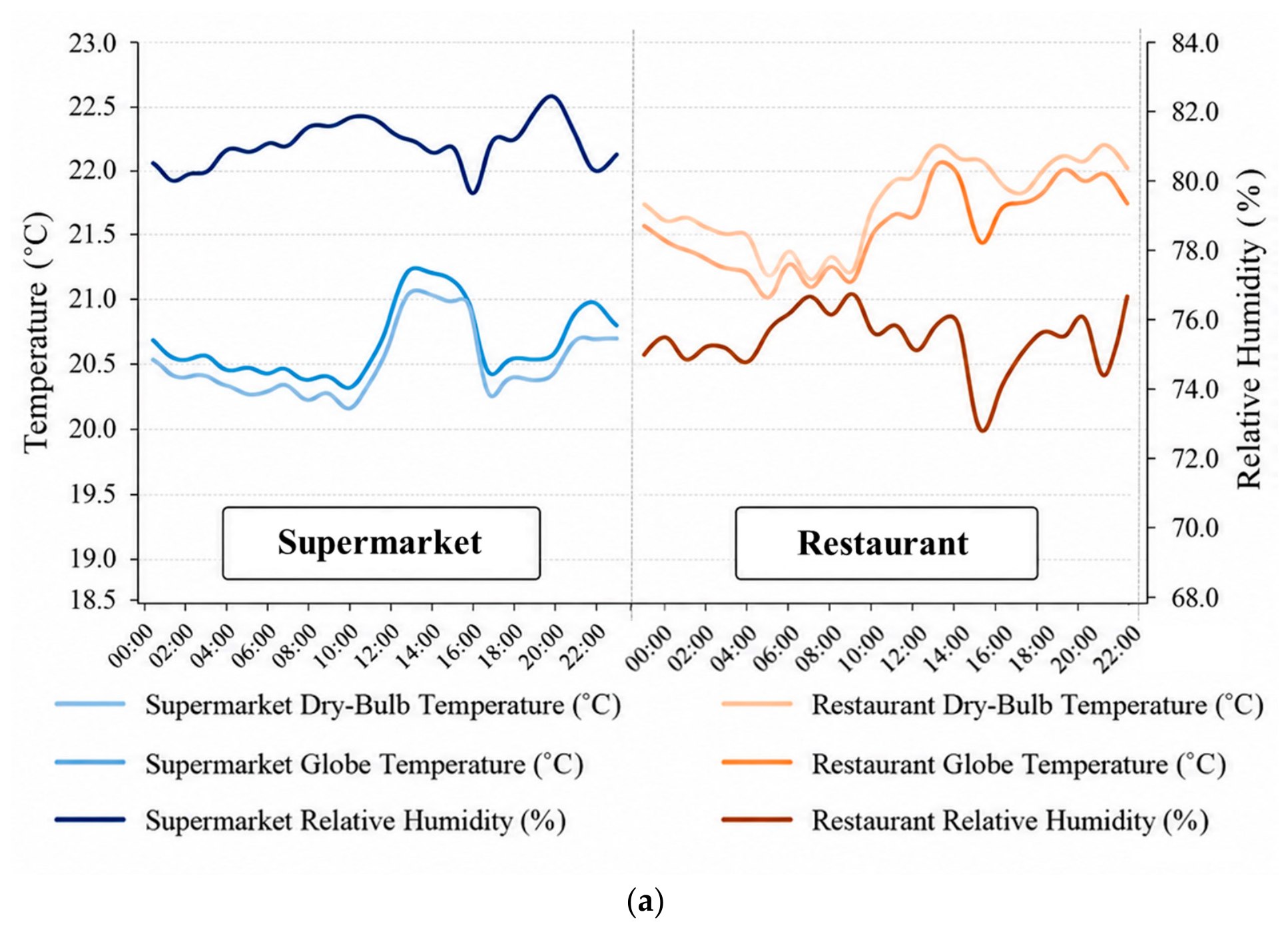
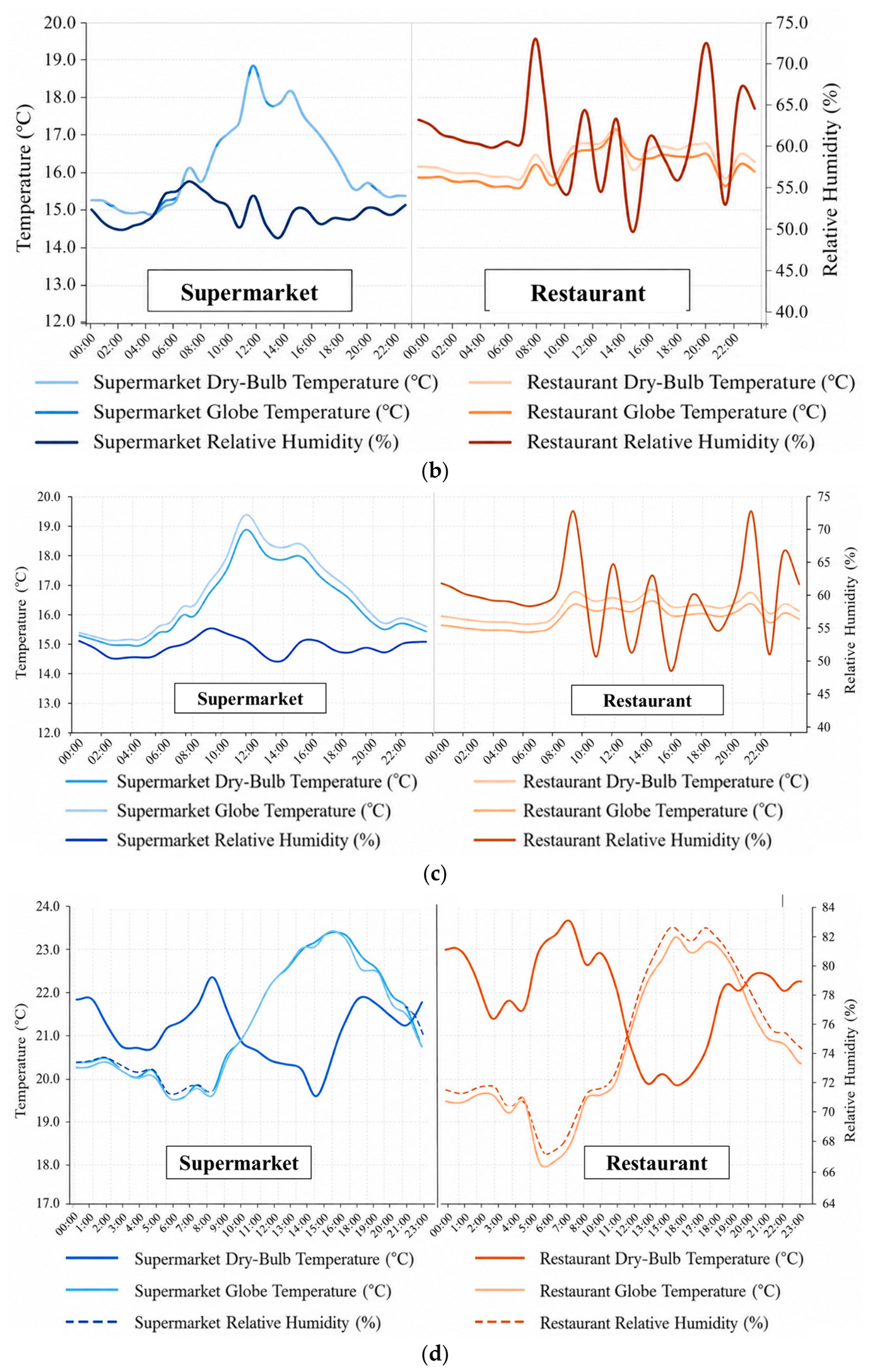
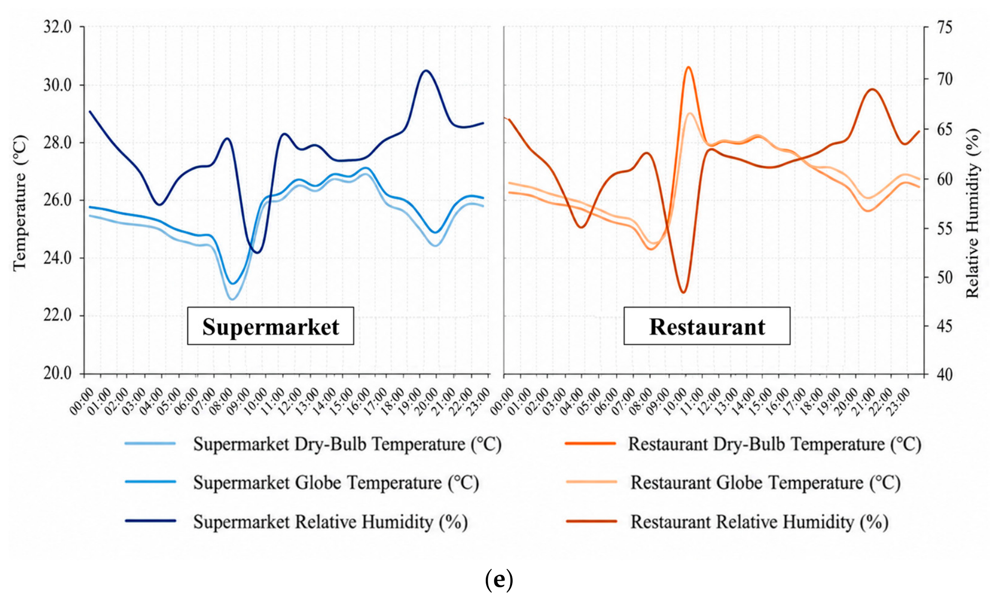
Figure 3 shows the 24 h indoor air temperature and relative humidity in the five service-area buildings. Figure 3a–e corresponds to Queshan, Machangyuan, Chabala, Ganzhuang, and Baoting, respectively. All cases exhibit a limited diurnal indoor temperature swing, within 5 °C. Queshan shows the smallest variation, below 3 °C, and the profiles remain relatively smooth under a free-running condition (Figure 3a). Machangyuan shows higher and more variable humidity in the restaurant than in other zones, which is consistent with cooking-related latent loads (Figure 3b). Chabala presents a pronounced disturbance during 08:00–09:00, when door opening induces a rapid indoor temperature drop in the non-heating period (Figure 3c). Ganzhuang maintains a stable indoor environment, with a mild temperature increase during 14:00–17:00 and a gradual humidity rise from morning to afternoon (Figure 3d). Baoting shows a daytime warming trend from 09:00 to 16:00 and irregular humidity fluctuations, which reflects the hot-humid climate and variable internal moisture loads (Figure 3e).

Figure 3. Measurement of indoor temperature and relative humidity in five service areas: (a) Queshan; (b) Machangyuan; (c) Chabala; (d) Ganzhuang; and (e) Baoting.

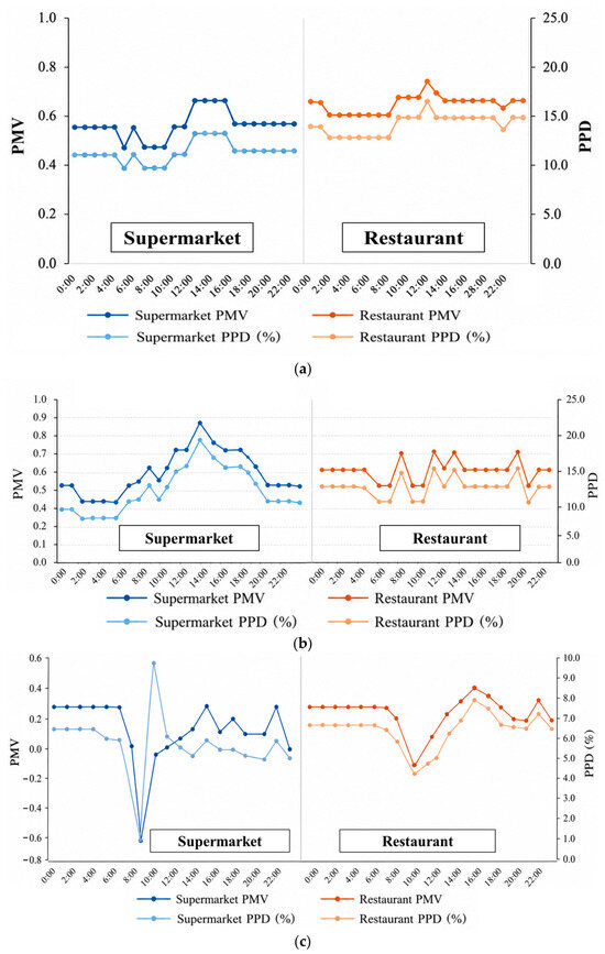
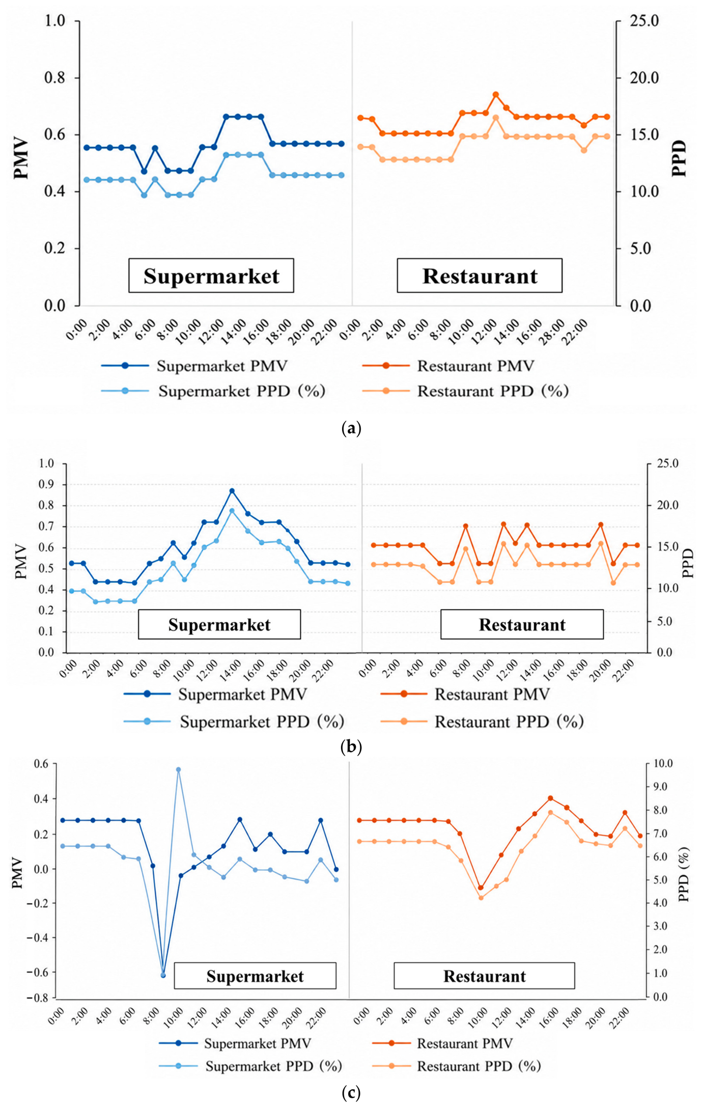
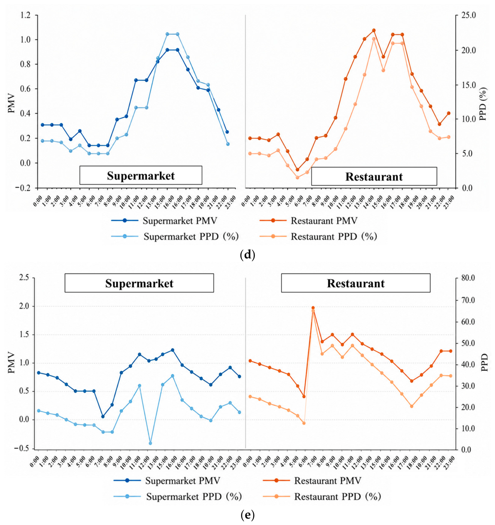
Figure 4 summarizes the thermal comfort results based on the PMV metric. Queshan shows PMV in the range 0.4–0.9, corresponding to a general slightly warm sensation. The supermarket zone presents lower temperature and higher humidity than the service counter and restaurant, and it achieves comparatively better comfort stability. Machangyuan shows a PMV between 0.3 and 0.9. The building is in the heating season, and comfort remains close to the acceptable band. Variations persist due to envelope heat transfer and frequent entrance opening. Chabala shows a distinct PMV response to infiltration. The rapid temperature drops during 08:00–09:00 in Figure 3c are followed by a pronounced PMV decrease in Figure 4c. Ganzhuang maintains acceptable comfort for most of the day, consistent with the mild climate and the modest need for active conditioning during the monitoring period. Baoting presents the least stable comfort. PMV approaches 1.8 during warm and humid periods, indicating that humidity control is a primary limitation in hot-humid service-area buildings.

Figure 4. PMV and PPD in five service areas: (a) Queshan; (b) Machangyuan; (c) Chabala; (d) Ganzhuang; and (e) Baoting.

The restaurant zone shows larger humidity variability than the retail zone across climates, and short-term operational events dominate comfort even when the diurnal indoor temperature swing is small, as demonstrated by Chabala in Figure 3c and Figure 4c.

4.2. Life-Cycle Carbon Emission Accounting of the Service Area

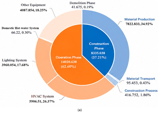
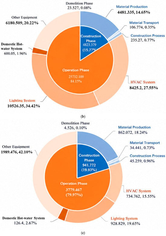
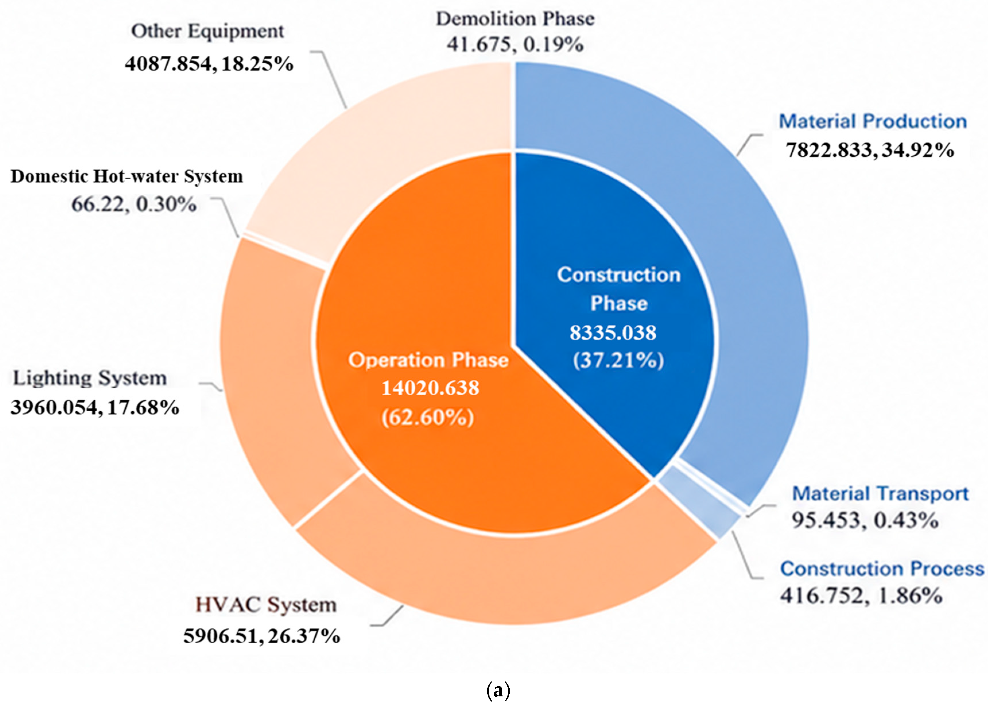
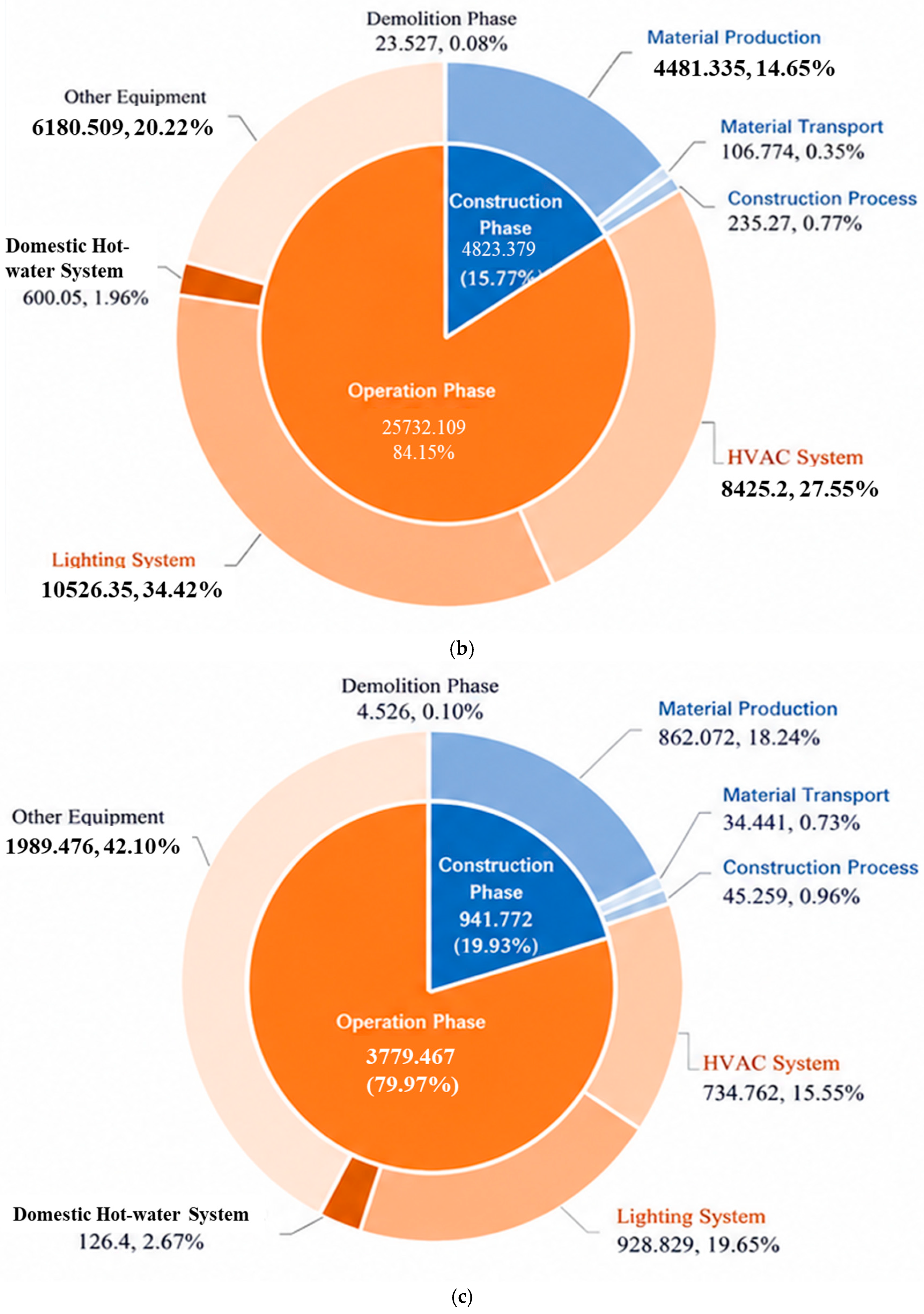
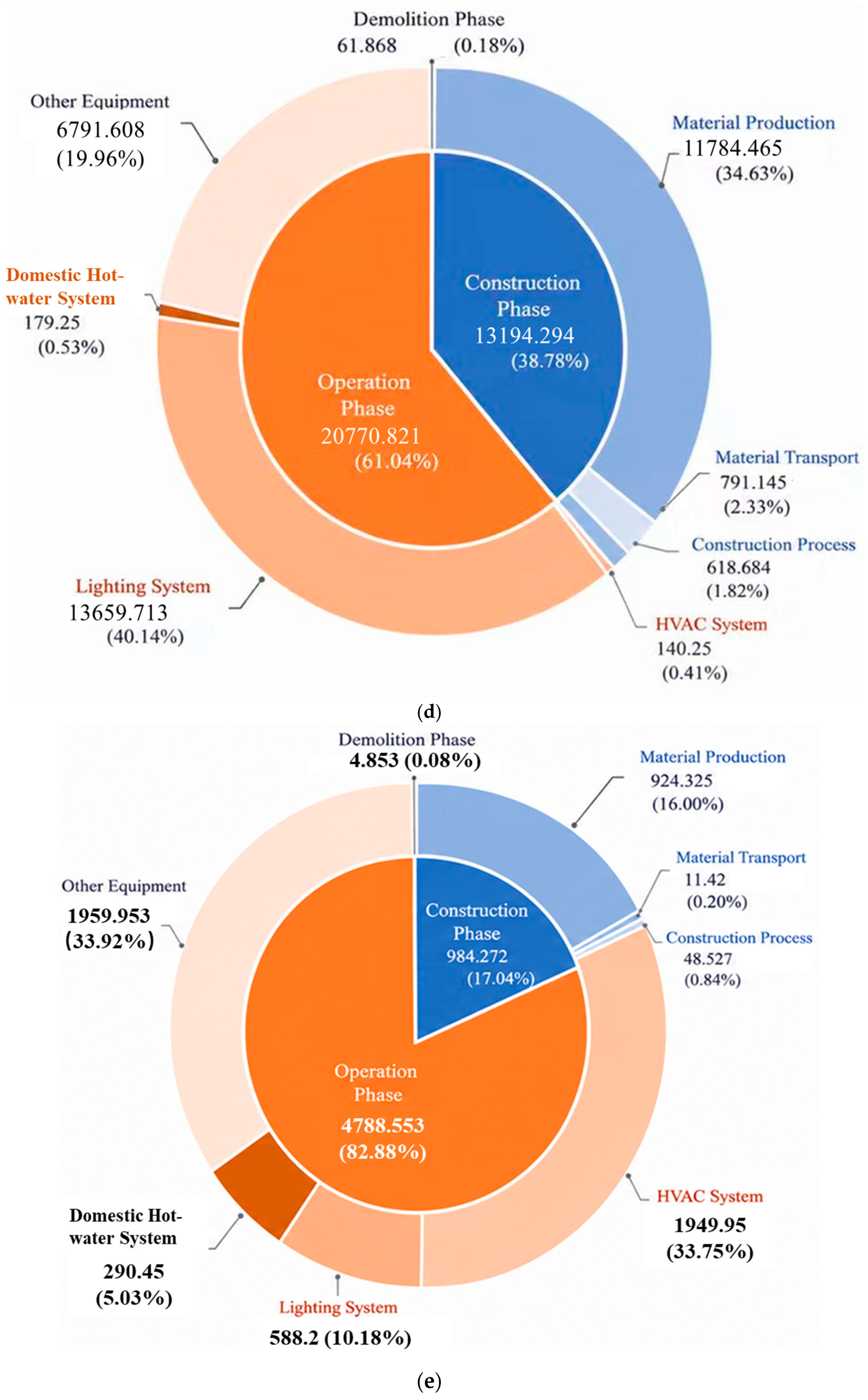
Table 5 summarizes the life-cycle carbon emissions of the integrated buildings in the five service areas. The total life-cycle emissions show a wide spread across climatic regions and operation modes. The Queshan case yields a total of 22,397.4 tCO₂ over 50 years, consisting of 8335.0 tCO₂ from construction, 14,020.6 tCO₂ from operation, and 41.7 tCO₂ from demolition. After accounting for on-site photovoltaics and vegetation sinks, the net emissions decrease to 10,077.9 tCO₂. The Machangyuan case shows a larger total of 30,579.0 tCO₂, mainly driven by operational emissions of 25,732.1 tCO₂, while construction and demolition contribute 4823.4 tCO₂ and 23.5 tCO₂, respectively. The Chabala case has a much smaller building-scale total. Construction, operation, and demolition are 941.8 tCO₂, 3779.5 tCO₂, and 4.5 tCO₂, respectively, and the renewable contribution remains limited, with only a marginal reduction reported. The Ganzhuang case shows a high total because of both a large construction-stage footprint and substantial operational demand. Construction, operation, and demolition are 13,194.3 tCO₂, 20,770.8 tCO₂, and 61.9 tCO₂, respectively, and the net result indicates a meaningful offset effect after renewables and sinks are considered. The Baoting case exhibits the lowest gross total among the five cases, with 989.1 tCO₂ from construction plus demolition and 4788.6 tCO₂ from operation. A large PV electricity yield leads to a strong offset, and the net life-cycle emissions become negative at −49,045.5 tCO₂.

Table 5. The full life-cycle carbon emissions of the service-area comprehensive buildings.

Service Area	Stage	Category	Carbon Emissions (tCO2)	Carbon Emissions (tCO2)	Carbon Sinks and Carbon Reduction (tCO2)	Total Carbon Emissions (tCO2)
Queshan	Construction	Materials production	7822.833	8335.038	12,322.5	10,077.853
		Materials transport	95.453
		Material processing	416.752
	Operational	HVAC	5906.51	14,020.64
		Lighting	3960.054
		Domestic hot water	66.22
		Other	4087.854
	Demolition	Remove	41.675	41.675
Machangyuan	Construction	Materials production	4481.335	4823.379		30,579.015
		Materials transport	106.774
		Material processing	235.27
	Operational	HVAC	8425.2	25,732.109
		Lighting	10,526.35
		Domestic hot water	600.05
		Other	6180.509
	Demolition	Remove	23.527	23.527
Chabala	Construction	Materials production	862.072	941.772	412.657	4313.108
		Materials transport	34.441
		Material processing	45.259
	Operational	HVAC	734.762	3779.467
		Lighting	928.829
		Domestic hot water	126.4
		Other	1989.476
	Demolition	Remove	4.526	4.526
Ganzhuang	Construction	Materials production	11,784.465	13,194.29	20,827.758	13,199.22
		Materials transport	791.145
		Material processing	618.684
	Operational	HVAC	140.25	20,770.82
		Lighting	13,659.713
		Domestic hot water	179.25
		Other	6791.608
	Demolition	Remove	61.868	61.868
Baoting	Construction	Materials production	924.325	984.272	54,823.163	−49,045.485
		Materials transport	11.42
		Material processing	48.527
	Operational	HVAC	1949.95	4788.553
		Lighting	588.2
		Domestic hot water	290.45
		Other	1959.953
	Demolition	Remove	4.853	4.853

To improve cross-case comparability, net life-cycle emission intensity is also normalized by floor area. The calculated values are 2865.2 kgCO₂e m⁻² for Queshan, 14,084.6 kgCO₂e m⁻² for Machangyuan, 3977.8 kgCO₂e m⁻² for Chabala, 4169.7 kgCO₂e m⁻² for Ganzhuang, and −57,853.0 kgCO₂e m⁻² for Baoting. The high intensity in Machangyuan reflects strong heating and lighting loads, whereas the negative value in Baoting results from large PV offsets relative to the small building area.

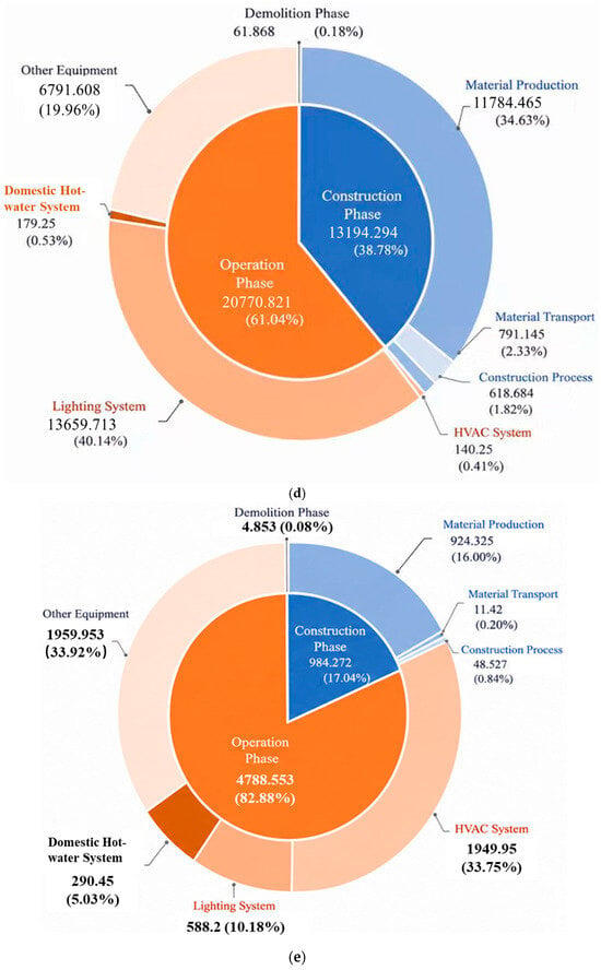
Figure 5 shows the contribution of each life-cycle component for the five cases. Operational emissions dominate the life-cycle profile in all service areas, while the internal composition of the operation stage varies by climate. In Queshan, HVAC is the largest operational source, and the construction stage remains non-negligible due to material production. In Machangyuan, the operational stage is driven by space heating and lighting, consistent with long heating periods and high lighting demand. In Chabala, “other electric equipment” becomes the largest operational contributor, while HVAC contributes less than in the severe-cold case, reflecting a shorter heating demand duration. In Ganzhuang, lighting dominates the operational stage, and its share reaches 65.8% of operation-stage emissions, which indicates that non-HVAC electricity use governs the carbon profile in the mild climate. In Baoting, HVAC remains the largest operational contributor, but the PV offset is sufficiently large to exceed the full life-cycle emissions, leading to a net-negative outcome.

Figure 5. Contribution of life-cycle carbon emissions by service area: (a) Queshan; (b) Machangyuan; (c) Chabala; (d) Ganzhuang; and (e) Baoting.

4.3. Orthogonal Experiment for Significance of Envelope-Related Drivers

An orthogonal experimental design is used to quantify the relative importance of five envelope-design factors on envelope-related carbon emissions [46]. The factors are building orientation, building height, south-facing window-to-wall ratio, external wall heat-transfer coefficient, and roof heat-transfer coefficient. Each factor has five levels. An L25 orthogonal array is adopted. The response variable is the life-cycle carbon emissions of the integrated building under each parameter combination. Table 6 defines the factors and level settings.

Table 6. Factors and levels used in the L25 orthogonal design.

Factors	Number	Horizontal Value
		Queshan	Machangyuan	Chabala	Baoting
Orientation (°)	A1	210	0	210	210
	A2	240	30	240	240
	A3	270	60	270	270
	A4	300	90	300	300
	A5	330	120	330	330
Building height (mm)	B1	7800	7200	6900	7800
	B2	8600	8200	7900	8800
	B3	9400	9200	8900	9800
	B4	10,200	10,200	9900	10,800
	B5	11,000	11,200	10,900	11,800
South-facing window-to-wall ratio (WWR)	C1	0.2	0.2	0.2	0.2
	C2	0.3	0.3	0.3	0.3
	C3	0.4	0.4	0.4	0.4
	C4	0.5	0.5	0.5	0.5
	C5	0.6	0.6	0.6	0.6
External wall heat-transfer coefficient (W/(m2·K))	D1	0.2	0.2	0.2	0.2
	D2	0.4	0.4	0.4	0.4
	D3	0.6	0.6	0.6	0.6
	D4	0.8	0.8	0.8	0.8
	D5	1	1	1	1
Roof heat-transfer coefficient (W/(m2·K))	E1	0.2	0.2	0.2	0.2
	E2	0.4	0.4	0.4	0.4
	E3	0.6	0.6	0.6	0.6
	E4	0.8	0.8	0.8	0.8
	E5	1	1	1	1

The five factors are selected because they are early stage design variables and directly affect envelope-related carbon emissions through both material demand and operational loads. The level ranges are determined from the baseline building dimensions, practical design limits, and the thermal transmittance values used in the carbon calculation. The L25 orthogonal array is used to evaluate the main effects of the five selected factors. However, it does not account for interaction effects among factors. This is acknowledged as a methodological limitation of the analysis.

The analysis of variance (ANOVA) for orthogonal test data is performed by calculating the F-values and significance levels of each factor to quantify their main effects on carbon emissions [47]. The ANOVA is carried out in the following steps:

• Sum of squares for each factor

  $$Q_A={\displaystyle \frac{1}{p}}\sum _{i=1}^m{\left(K_i\right)}^2-{\displaystyle \frac{1}{mp}}{\left(\sum _{i=1}^m\sum _{j=1}^p{x}_{ij}\right)}^2$$

  (12)
• Total sum of squares

  $$Q_T=\sum _{i=1}^m\sum _{j=1}^p{\left(x_{ij}-x\right)}^2$$

  (13)

  $$Q_T=Q_A+Q_B+\dots +Q_N+Q_e$$

  (14)
• Calculation of degrees of freedom

  $$f_T=n-1$$

  (15)

  $$f_A=m-1$$

  (16)

  $$f_e=n-m$$

  (17)
• Calculation of mean squares

  $${MS}_A={\displaystyle \frac{Q_A}{f_A}}$$

  (18)

  $${MS}_e={\displaystyle \frac{Q_e}{f_e}}$$

  (19)
• F-test for F-ratio

  $$F={\displaystyle \frac{{MS}_A}{{MS}_e}}$$

  (20)
• Test for the significance of factors

The corresponding significance value (Sig) is determined by referring to the F-distribution table based on the calculated F-value. If Sig < 0.05, the factor is considered to have a significant effect on the test results. If Sig > 0.05, the factor is considered to have no significant effect on the results [48].

The results of the analysis of factors influencing carbon emissions across the four climate zones are shown in Table 7. The orthogonal analysis indicates that, in Queshan, the factor importance ranks as building height > roof > orientation > wall > south-facing WWR. The optimal low-carbon combination is a north azimuth of 270°, a building height of 7800 mm, a south-facing WWR of 0.4, a wall heat-transfer coefficient of 0.8 W·m⁻²·K⁻¹, and a roof heat-transfer coefficient of 0.4 W·m⁻²·K⁻¹. The effect of WWR is relatively weak in this climate within the tested range.

Table 7. Results of orthogonal experiments in different service areas.

Service Area	Parameters	${\mathit{Q}}_{\mathit{T}}$	Flexibility	${\mathit{M}\mathit{S}}_{\mathit{e}}$	F	Sig
Queshan	A	12.109	4	3.027	152.624	<0.001
	B	1594.219	4	398.555	20,093.85	<0.001
	C	0.116	4	0.029	1.46	0.361
	D	11.919	4	2.98	150.224	<0.001
	E	28.25	4	7.063	356.07	<0.001
Machangyuan	A	461.571	4	115.393	84.095	<0.0001
	B	2732.921	4	683.23	497.917	<0.0001
	C	620.617	4	115.154	113.072	<0.0001
	D	1320.503	4	330.126	240.585	<0.0001
	E	1699.069	4	424.767	309.557	<0.0001
Chabala	A	1.491	4	0.373	27.637	0.004
	B	127.25	4	31.813	2359.363	<0.001
	C	0.841	4	0.21	15.6	<0.001
	D	5.196	4	1.299	96.349	<0.001
	E	34.939	4	8.735	647.81	<0.001
Baoting	A	10.605	4	2.651	15.598	0.010
	B	159.872	4	39.968	235.142	<0.001
	C	0.828	4	0.207	1.218	0.427
	D	2.902	4	0.725	4.268	0.094
	E	2.054	4	0.514	3.021	0.155

In Machangyuan, the ranking is building height > roof > wall > south-facing WWR > orientation. The optimal combination is a north azimuth of 90°, a building height of 7200 mm, a south-facing WWR of 0.2, and a wall and roof heat-transfer coefficient of 0.2 W·m⁻²·K⁻¹. Envelope thermal transmittance has a strong effect, while the effect of orientation is smaller.

In Chabala, the ranking is building height > roof > wall > orientation > south-facing WWR. The optimal combination is a north azimuth of 210°, a building height of 6900 mm, a south-facing WWR of 0.2, and a wall and roof heat-transfer coefficient of 0.2 W·m⁻²·K⁻¹. These results highlight the priority of reducing heat losses through the envelope in cold climates.

In Baoting, the ranking is building height > orientation > wall > roof > south-facing WWR. The optimal combination is a north azimuth of 60°, a building height of 7800 mm, a south-facing WWR of 0.4, a wall heat-transfer coefficient of 0.8 W·m⁻²·K⁻¹, and a roof heat-transfer coefficient of 0.4 W·m⁻²·K⁻¹.

Across all climatic regions, building height is the dominant driver of life-cycle carbon emissions. Reducing height lowers both embodied emissions and operational emissions. Height optimization should therefore be prioritized, while maintaining functional requirements.

4.4. Carbon Emission Control Strategies

The results presented in Section 4.2 and Section 4.3 indicate that both the dominant emission sources and the sensitivity of design parameters vary across climatic regions. Based on these findings, climate-adaptive carbon reduction strategies are developed for each service area. The proposed measures are summarized in Table 8.

Table 8. Climate-adaptive carbon reduction strategies for different service areas.

Service Area	Climate-Adaptive Mitigation Measures
Queshan	Height reduction to the preferred level, roof insulation improvement, HVAC scheduling, lighting control, and PV self-consumption
Machangyuan	Height reduction, roof and wall insulation enhancement, thermal-bridge and airtightness control, heating-side management, and PV utilization
Chabala	Height reduction, envelope thermal optimization, entrance buffering, infiltration control, and PV utilization
Ganzhuang	Daylighting system, lighting schedule optimization, bifacial PV modules, and vegetation carbon sink
Baoting	Orientation optimization, solar shading, humidity-oriented HVAC control, ventilation management, and PV utilization

The building height reduction is recommended for all climatic regions because of its consistent influence on both embodied and operational carbon emissions. In the severe-cold and cold regions, additional emphasis is placed on roof and wall insulation to reduce heating demand. For the hot-summer and cold-winter region, a balanced strategy combining geometry optimization, envelope improvement, and operational control is adopted. In the hot-summer and warm-winter region, orientation optimization, solar control, and humidity-oriented operation become more important. Renewable-energy utilization is incorporated into all service areas and serves as the primary carbon-offset measure.

The carbon reduction performance of the optimized schemes is summarized in Table 9. The reduction ratio ranges from 40.35% to 87.94% for the northern service areas. Queshan, Machangyuan, Chabala, and Ganzhuang achieve carbon reductions of 5121.0, 12,336.0, 3792.8, and 16,741.9 tCO₂e, respectively. Among these cases, Chabala exhibits the highest reduction ratio at 87.94%, indicating the substantial benefits of combining envelope optimization with renewable energy utilization.

Table 9. Carbon reduction performance of optimized schemes.

Service Area	Baseline Emissions (tCO2)	Optimized Emissions (tCO2)	Reduction (tCO2)	Reduction Ratio (%)
Queshan	10,077.853	4956.859	5120.994	50.82
Machangyuan	30,579.015	18,242.969	12,336.046	40.35
Chabala	4313.108	520.339	3792.769	87.94
Ganzhuang	30,579.015	13,837.135	16,741.88	54.75
Baoting	−49,045.485	−50,654.863	1609.378	3.16

The contribution of mitigation measures varies among climatic regions. In Machangyuan and Chabala, building height reduction and envelope insulation optimization provide significant reductions by lowering heating demand. In Ganzhuang, daylighting systems, bifacial photovoltaic modules, and vegetation carbon sinks contribute substantially to the overall reduction. These results indicate that passive design measures effectively reduce energy demand, while renewable energy systems provide additional carbon offsets.

Baoting exhibits a different carbon reduction pattern. Owing to abundant solar resources and renewable energy utilization, the service area maintains a net-negative carbon balance before and after optimization. The optimized scheme further reduces net emissions by 1609.4 tCO₂e, corresponding to a reduction ratio of 3.16%. Although the relative reduction is smaller than that observed in other regions, the building has already reached a highly optimized low-carbon state.

From an engineering perspective, measures with low implementation barriers should be prioritized first, such as height control in new designs, lighting scheduling, entrance buffering, and HVAC set-point management. PV installation has higher initial cost but provides the largest long-term offset where roof area and solar resources are sufficient. Detailed life-cycle cost analysis is not included and should be incorporated before large-scale implementation.

The baseline net emissions in Table 9 refer to the net carbon balance before implementing the service-area-specific optimization package. They should not be confused with the gross life-cycle emissions in Table 5.

5. Discussion

This study extends existing building life-cycle carbon assessments by focusing on highway service-area buildings and by comparing representative cases across different climatic regions. The results are broadly consistent with previous building LCA studies showing the dominance of operational emissions, but they further indicate that service-area buildings have distinct end-use profiles because of long operating hours, catering activities, retail loads, and large PV deployment potential. These findings support the need for climate-specific strategies rather than a uniform mitigation package.

Several limitations remain. First, the analysis is based on five representative cases, so the results should be interpreted as climate-zone case evidence rather than national statistical averages. Second, the indoor thermal measurements cover typical 24 h operating periods, and seasonal monitoring is not available. Third, recurrent emissions from major maintenance, equipment replacement, and renovation are not quantified because consistent records were unavailable. Fourth, PV offsets, vegetation sinks, and grid emission factors are treated using simplified long-term assumptions. Future work should combine long-term monitoring, dynamic building simulation, time-varying grid scenarios, and life-cycle cost analysis to refine carbon-neutral design guidelines for highway service areas.

6. Conclusions

This study investigates the life-cycle carbon emissions of highway service-area buildings in five climatic regions of China and evaluates climate-adaptive mitigation strategies. The main conclusions are as follows.

• Operational emissions dominate the life-cycle carbon emissions of highway service-area buildings, accounting for approximately 61–84% of total emissions. Heating, cooling, lighting, and auxiliary electricity consumption are the primary emission sources.
• Building height is identified as the most influential design parameter in all climatic regions. In severe-cold and cold regions, roof and wall thermal performance also have significant impacts on life-cycle carbon emissions.
• Climate-adaptive optimization measures effectively reduce carbon emissions. The optimized schemes achieve carbon reduction ratios of 50.82%, 40.35%, 87.94%, and 54.75% in Queshan, Machangyuan, Chabala, and Ganzhuang service areas, respectively.
• Renewable energy utilization substantially improves carbon mitigation performance. In the Baoting service area, photovoltaic generation combined with vegetation carbon sinks maintains a net-negative carbon balance, demonstrating the potential for developing low-carbon and carbon-negative highway service-area buildings in regions with abundant solar resources.
• For designers and highway operators, the practical pathway is to first reduce demand through passive and operational measures, and then use PV and site-level sinks to offset the remaining emissions.

References

- Fawzy, S.; Osman, A.I.; Doran, J.; Rooney, D.W. Strategies for mitigation of climate change: A review. Environ. Chem. Lett. 2020, 18, 2069–2094. [Google Scholar] [CrossRef] [Scilit]
- Chiang, W.-Y.; Chen, Y.-A.; Chen, V.Y.; Tsou, W.-L.; Chen, C.-H.; Tsai, H.-C.; Sun, C.-Y. Urban Renewal as a Passive Heat Adaptation Strategy: Distance–Decay and Spatial Extent of Microclimate Effects in High-Density Subtropical Cities. Atmosphere 2026, 17, 470. [Google Scholar]
- Yigitcanlar, T.; Kamruzzaman, M. Investigating the interplay between transport, land use and the environment: A review of the literature. Int. J. Environ. Sci. Technol. 2014, 11, 2121–2132. [Google Scholar] [CrossRef] [Scilit]
- Bai, H.; Qi, D. Tripartite Evolutionary Game for Carbon Reduction in Highway Service Areas: Evidence from Xinjiang, China. Sustainability 2025, 17, 10145. [Google Scholar] [CrossRef] [Scilit]
- Wang, J.; Li, Y.; Mai, J.; Yuan, M.; Liu, Z. Highway Typical Scenario Operation and Maintenance Energy Demand Forecasting. Sustainability 2025, 17, 1929. [Google Scholar] [CrossRef] [Scilit]
- Boarnet, M.G. Infrastructure services and the productivity of public capital: The case of streets and highways. Natl. Tax J. 1997, 50, 39–57. [Google Scholar] [CrossRef] [Scilit]
- Kreminski, R.; Hirsch, A.H.; Boand, J. Assessment of Colorado Department of Transportation Rest Areas for Sustainability Improvements and Highway Corridors and Facilities for Alternative Energy Use; Colorado State University: Pueblo, CO, USA, 2011. [Google Scholar]
- Yang, W.; Pan, J. The role of vegetation carbon sequestration in offsetting energy carbon emissions in the Yangtze River Basin, China. Environ. Dev. Sustain. 2024, 26, 22689–22714. [Google Scholar]
- Wu, X.; Wang, Y.; Deng, S.; Su, P. Climate-responsive design of photovoltaic façades in hot climates: Materials, technologies, and implementation strategies. Buildings 2025, 15, 1648. [Google Scholar] [CrossRef] [Scilit]
- Garimella, S. Innovations in energy efficient and environmentally friendly space-conditioning systems. Energy 2003, 28, 1593–1614. [Google Scholar] [CrossRef] [Scilit]
- McIlvenny, H.; Clements, A.; Helyar, S. Sediment properties influence seagrass sedimentary carbon stocks, challenging uniform blue carbon accounting. Front. Mar. Sci. 2026, 13, 1809172. [Google Scholar] [CrossRef] [Scilit]
- Xiong, L.; Wang, M.; Mao, J.; Huang, B. A review of building carbon emission accounting methods under low-carbon building background. Buildings 2024, 14, 777. [Google Scholar] [CrossRef] [Scilit]
- Baustert, P.; Navarrete Gutiérrez, T.; Gibon, T.; Chion, L.; Ma, T.-Y.; Mariante, G.L.; Klein, S.; Gerber, P.; Benetto, E. Coupling activity-based modeling and life cycle assessment—A proof-of-concept study on cross-border commuting in Luxembourg. Sustainability 2019, 11, 4067. [Google Scholar]
- Muhammed, S.; Chaudhry, H.N.; Santiago, I.M.C. An Analytical Study of Horizontal Adaptations of Vernacular Barjeel (Windcatcher) in the Desert Architecture of the Gulf Region. Architecture 2026, 6, 43. [Google Scholar] [CrossRef] [Scilit]
- Albelwi, N. DT-LCAF: Digital Twin-Enabled Life Cycle Assessment Framework for Real-Time Embodied Carbon Optimization in Smart Building Construction. Sustainability 2026, 18, 2321. [Google Scholar]
- Champions, U.C.C.H.-L. The Breakthrough Agenda Report 2023; IEA: Paris, France, 2023. [Google Scholar]
- Janjic, M. The Role of the International Energy Agency (IEA) in Global Energy Governance; University of Piraeus: Piraeus, Greece, 2025. [Google Scholar]
- Lausselet, C.; Ellingsen, L.A.W.; Strømman, A.H.; Brattebø, H. A life-cycle assessment model for zero emission neighborhoods. J. Ind. Ecol. 2020, 24, 500–516. [Google Scholar]
- Terrill, T.J.; Rasmussen, B.P. An evaluation of HVAC energy usage and occupant comfort in religious facilities. Energy Build. 2016, 128, 224–235. [Google Scholar] [CrossRef] [Scilit]
- Zhou, Y.; Wu, J.; Wang, R.; Shiochi, S. Energy simulation in the variable refrigerant flow air-conditioning system under cooling conditions. Energy Build. 2007, 39, 212–220. [Google Scholar] [CrossRef] [Scilit]
- Zhang, X.; Wang, F. Life-cycle assessment and control measures for carbon emissions of typical buildings in China. Build. Environ. 2015, 86, 89–97. [Google Scholar] [CrossRef] [Scilit]
- Ayalew, B.S.; Andrzejczyk, R. Recent Advancements in Latent Thermal Energy Storage and Their Applications for HVAC Systems in Commercial and Residential Buildings in Europe—Analysis of Different EU Countries’ Scenarios. Energies 2025, 18, 4000. [Google Scholar] [CrossRef] [Scilit]
- Karapidakis, E.; Nikologiannis, M.; Markaki, M.; Kouzoukas, G.; Yfanti, S. Enhancing renewable energy integration and implementing EV charging stations for sustainable electricity in Crete’s supermarket chain. Energies 2025, 18, 754. [Google Scholar] [CrossRef] [Scilit]
- Creutzig, F.; Agoston, P.; Goldschmidt, J.C.; Luderer, G.; Nemet, G.; Pietzcker, R.C. The underestimated potential of solar energy to mitigate climate change. Nat. Energy 2017, 2, 17140. [Google Scholar] [CrossRef] [Scilit]
- Bai, L.; Song, B.; Yang, L. Developing the new thermal climate zones of China for building energy efficiency using the cluster approach. Atmosphere 2022, 13, 1498. [Google Scholar] [CrossRef] [Scilit]
- Hamdane, S.; Pires, L.C.; Gaspar, P.D.; Silva, P.D. Innovative Strategies for Thermal Energy Optimization and Renewable Energy Integration in Net-Zero-Energy Buildings: A Comprehensive Review. Energies 2024, 17, 5664. [Google Scholar]
- Chen, H.; Wang, L.; Wang, Y.; Ni, Z.; Xia, B.; Qiu, R. New perspective to evaluate the carbon offsetting by urban blue-green infrastructure: Direct carbon sequestration and indirect carbon reduction. Environ. Sci. Technol. 2024, 58, 12966–12975. [Google Scholar] [CrossRef] [Scilit] [PubMed]
- Zhao, L.; Guo, C.; Chen, L.; Qiu, L.; Wu, W.; Wang, Q. Using BIM and LCA to calculate the life cycle carbon emissions of inpatient building: A case study in China. Sustainability 2024, 16, 5341. [Google Scholar] [CrossRef] [Scilit]
- Gao, S.; Liu, X.; Lu, C.; Zhang, H.; Wang, X.; Kong, Y. Quantitative analysis of carbon emissions from highway construction based on life cycle assessment. Sustainability 2024, 16, 5897. [Google Scholar] [CrossRef] [Scilit]
- Han, Y.; Li, J.; Guo, X.; Sun, J. Research on Integrated Energy Utilization of Desert Expressway Service Area Buildings. Energies 2026, 19, 1387. [Google Scholar] [CrossRef] [Scilit]
- Yu, Q.; Zhang, Y.; Chu, Z.; Zhang, S.; Shen, Z.; Ma, Z. Assessment of Photovoltaic Power Generation Potential in Chinese Expressway Service Areas. Energies 2025, 18, 6209. [Google Scholar] [CrossRef] [Scilit]
- Ibn-Mohammed, T.; Greenough, R.; Taylor, S.; Ozawa-Meida, L.; Acquaye, A. Operational vs. embodied emissions in buildings—A review of current trends. Energy Build. 2013, 66, 232–245. [Google Scholar] [CrossRef] [Scilit]
- Wang, C.; Wang, Y.; Tong, X.; Ulgiati, S.; Liang, S.; Xu, M.; Wei, W.; Li, X.; Jin, M.; Mao, J. Mapping potentials and bridging regional gaps of renewable resources in China. Renew. Sustain. Energy Rev. 2020, 134, 110337. [Google Scholar] [CrossRef] [Scilit]
- Moschetti, R.; Homaei, S.; Taveres-Cachat, E.; Grynning, S. Assessing responsive building envelope designs through robustness-based multi-criteria decision making in zero-emission buildings. Energies 2022, 15, 1314. [Google Scholar]
- ISO 7730:2025; Ergonomics of the Thermal Environment-Analytical Determination and Interpretation of Thermal Comfort Using Calculation of the PMV and PPD Indices and Local Thermal Comfort Criteria. International Organization for Standardization: Geneva, Switzerland, 2025.
- Zhang, Z.; Liu, R. Carbon emissions in the construction sector based on input-output analyses. Qinghua Daxue Xuebao/J. Tsinghua Univ. 2013, 53, 53–57. [Google Scholar]
- Zhao, Y.; Liu, L.; Yu, M. Comparison and analysis of carbon emissions of traditional, prefabricated, and green material buildings in materialization stage. J. Clean. Prod. 2023, 406, 137152. [Google Scholar] [CrossRef] [Scilit]
- Lu, K.; Deng, X.; Zhang, Y.; Jiang, X.; Cheng, B.; Tam, V.W. Extensible carbon emission factor database: Empirical study for the Chinese construction industry. Environ. Sci. Pollut. Res. 2024, 31, 41482–41501. [Google Scholar]
- Kargulewicz, I.; Chłopek, Z.; Waśniewska, S. Energy-related carbon dioxide emission factors from combustion of gaseous methane fuels. Environ. Prot. Nat. Resour. 2024, 34, 92–104. [Google Scholar]
- Fan, F.; Lei, Y. Factor analysis of energy-related carbon emissions: A case study of Beijing. J. Clean. Prod. 2017, 163, S277–S283. [Google Scholar] [CrossRef] [Scilit]
- Hammond, G.P.; Jones, C.I. Embodied energy and carbon in construction materials. Proc. Inst. Civ. Eng.-Energy 2008, 161, 87–98. [Google Scholar] [CrossRef] [Scilit]
- GB/T 51366-2019; Standard for Building Carbon Emission Calculation. China Architecture & Building Press: Beijing, China, 2019.
- Pan, W.; Li, K.; Teng, Y. Rethinking system boundaries of the life cycle carbon emissions of buildings. Renew. Sustain. Energy Rev. 2018, 90, 379–390. [Google Scholar] [CrossRef] [Scilit]
- Huxley, O.; Taylor, J.; Everard, A.; Briggs, J.; Tilley, K.; Harwood, J.; Buckley, A. The uncertainties involved in measuring national solar photovoltaic electricity generation. Renew. Sustain. Energy Rev. 2022, 156, 112000. [Google Scholar] [CrossRef] [Scilit]
- Dong, L.; Wang, Y.; Ai, L.; Cheng, X.; Luo, Y. A review of research methods for accounting urban green space carbon sinks and exploration of new approaches. Front. Environ. Sci. 2024, 12, 1350185. [Google Scholar] [CrossRef] [Scilit]
- Liu, Z.A.; Hou, J.; Zhang, L.; Dewancker, B.J.; Meng, X.; Hou, C. Research on energy-saving factors adaptability of exterior envelopes of university teaching-office buildings under different climates (China) based on orthogonal design and EnergyPlus. Heliyon 2022, 8, e10056. [Google Scholar] [PubMed]
- Armstrong, R.A.; Eperjesi, F.; Gilmartin, B. The application of analysis of variance (ANOVA) to different experimental designs in optometry. Ophthalmic Physiol. Opt. 2002, 22, 248–256. [Google Scholar] [PubMed]
- Bayer, F.P.; Gander, M.; Kuster, B.; The, M. CurveCurator: A recalibrated F-statistic to assess, classify, and explore significance of dose–response curves. Nat. Commun. 2023, 14, 7902. [Google Scholar] [PubMed]
Disclaimer/Publisher’s Note: The statements, opinions and data contained in all publications are solely those of the individual author(s) and contributor(s) and not of MDPI and/or the editor(s). MDPI and/or the editor(s) disclaim responsibility for any injury to people or property resulting from any ideas, methods, instructions or products referred to in the content. |
© 2026 by the authors. Licensee MDPI, Basel, Switzerland. This article is an open access article distributed under the terms and conditions of the Creative Commons Attribution (CC BY) license.