Research on Strategies to Enhance the Resilience of Urban Power-Transportation Systems by Considering Mobile Energy Storage in Severe Sandstorm Environments

Abstract

With the increasing frequency of extreme weather events, the vulnerability of urban power-transportation systems in severe dust storm conditions has become increasingly apparent. Addressing the shortcomings of existing research regarding the quantitative assessment and enhancement of system resilience, this paper proposes a set of strategies and methods for evaluating and improving the resilience of urban power-transportation systems under severe dust storm conditions, taking mobile energy storage into account. The study first establishes a multidimensional failure probability model for severe dust storm conditions: on the power grid side, it comprehensively considers fluctuations in renewable energy output, wind speed variations, and line insulation performance to propose a probabilistic failure model that accounts for the sand accumulation effect; on the transportation side, it considers road visibility and traffic flow to propose an improved BPR traffic flow model, using the Floyd algorithm to plan MES travel routes. Fault scenarios are generated using the Monte Carlo algorithm, and multidimensional system performance metrics for the power grid–road network-coupled nodes are established. A quantification method for resilience metrics applicable to urban power-transportation systems is proposed based on the ΦΛEΠ resilience index. Furthermore, a multi-objective, multi-stage resilience enhancement strategy for urban power-transportation systems that incorporates mobile energy storage is proposed using the NSGA-II algorithm. Finally, the effectiveness of the proposed optimization strategy was verified through coupled simulation cases using the IEEE-33 node test system and the Sioux Falls network. The results demonstrate that the proposed optimization strategy can significantly enhance system resilience under different optimization objectives.

1. Introduction

In 2025, the Ministry of Housing and Urban-Rural Development, together with eight other departments, jointly issued the Action Plan (2025–2027) for Implementing the “Opinions of the General Office of the CPC Central Committee and the General Office of the State Council on Promoting the Construction of New Urban Infrastructure and Building Resilient Cities,” to advance the development of new urban infrastructure characterized by digitalization, networking, and intelligence, and to enhance urban risk prevention, control, and governance capabilities [1]. The Outline of the 14th Five-Year Plan [2] explicitly calls for the development of new-type cities capable of withstanding disasters through their own capabilities, mitigating losses, rationally allocating resources for rapid recovery, and learning from past events to enhance their adaptability. As the two core systems for maintaining normal urban operations, research on methods to enhance the resilience of the power and transportation systems has gradually become a research hotspot [3].

In recent years, the rapid growth in the number of electric vehicles has led to increasingly close interdependence between the power and transportation systems. On the one hand, the interaction between these two systems increases the risk of cascading failures: a failure in either system can propagate to the other through coupling points, while the recovery process for either system may be constrained by the limited resources of the other, thereby delaying the restoration process. On the other hand, improved coordination between the two systems helps enhance a city’s ability to function normally during extreme events. Therefore, strengthening the resilience of urban power-transportation systems is an urgent priority to cope with increasingly frequent extreme weather events. In April 2025, a severe sandstorm affected a total of eight provinces and municipalities—including Beijing, Hebei, Shanxi, Inner Mongolia, Henan, Gansu, and Xinjiang—impacting 106 road sections [4]. In 2021, widespread sandstorms occurred in regions with significant renewable energy installations, such as Hebei, Shanxi, and Inner Mongolia, resulting in a substantial decline in photovoltaic power generation [5]. The impact of extreme weather on urban power-transportation systems is becoming increasingly severe. Traditional reliability metrics are insufficient to describe a system’s performance throughout the entire process of extreme events, damage, and recovery. Therefore, there is an urgent need to establish more comprehensive resilience assessment metrics to characterize dynamic features such as the extent of damage, the state of damage, and the speed of recovery, in order to build more resilient urban power-transportation systems and ensure the normal functioning of overall social systems.

Regarding research on the assessment and enhancement strategies for power system resilience, Reference [6] proposes two key indicators for evaluating grid resilience: “resilience risk factors” and “grid infrastructure density”. Reference [7] systematically reviews the power system resilience assessment framework and explores methods for enhancing power system resilience across three stages: fault prevention, fault response, and fault recovery. The aforementioned studies all focus on a single power grid and do not address the coupled effects on transportation networks. Reference [8] proposes an optimal pre-disaster deployment plan for mobile power sources and a post-disaster strategy for the coordinated dispatch of multiple emergency resources, providing a reference for enhancing urban power grid resilience; however, the dispatch of mobile power sources in this study is constrained by travel times on the road network. Regarding the assessment and enhancement strategies for transportation system resilience, Reference [9] proposes a road network performance evaluation model that uses an improved cellular traffic model to simulate traffic distribution and employs resilience as a performance metric; however, this model does not account for the feedback of power outages on EV charging behavior. Reference [10] quantifies the temporal reliability of highway passenger transport networks using the ratio of travel times during peak hours to those during free-flow conditions; however, it focuses on normal traffic fluctuations and does not account for the impact of extreme weather. Reference [11] summarizes methods for assessing transport network resilience and enhancement strategies, and catalogs commonly used models and optimization methods, but does not address coupling with the power system. Regarding urban power-transportation systems, most existing studies adopt a single-perspective approach, focusing on modeling either the power grid or the transportation network while simplifying the other system. While some studies have constructed two-level optimization models, they face serious challenges such as the curse of dimensionality and low solution accuracy. Additionally, due to differences in operational scales between the two systems, it is difficult to address both simultaneously during coordinated control; therefore, how to achieve dynamic adjustment of resource control strategies remains a major challenge [12,13,14,15,16].

As a typical extreme weather event characterized by low probability and high risk, severe dust storms pose a serious threat to the normal operation of urban power and transportation systems. If vulnerable components of the system are damaged by extreme dust storms, this could trigger widespread power outages in distribution grids and a drastic decline in the capacity of transportation networks, thereby posing a significant threat to socioeconomic operations and public safety. Therefore, there is an urgent need to effectively assess the resilience of urban power-transportation systems under severe sandstorm conditions and to formulate strategies for enhancing resilience. Addressing the shortcomings of existing research in the quantitative assessment of coupled systems and multi-stage collaborative optimization, the main contributions of this paper are as follows: (1) An urban power-transportation system model was established. Probability models for power system failures and transportation system failures under extreme sandstorm conditions were developed, and a multi-dimensional failure probability generation framework for coupled systems under sandstorm scenarios was constructed, enabling a unified characterization of the coupled failure process of the power grid and transportation network. (2) A resilience assessment method suitable for urban power-transportation systems is proposed. Comprehensive performance indicators are constructed from three dimensions—the power grid side, the road network side, and the coupling nodes—addressing the issue that single-system resilience indicators cannot reflect the interactive effects of coupled systems. (3) A three-phase resilience enhancement strategy—covering pre-disaster, during-disaster, and post-disaster phases—was proposed, incorporating mobile energy storage. With the objectives of minimizing total expected costs, minimizing power restoration time for the power grid, and minimizing expected travel time for the road network, the strategy was solved using the NSGA-II algorithm, achieving a balance between economic efficiency and recovery efficiency.

2. A Probability Model for Failures in Urban Power and Transportation Systems During Severe Sandstorms

Severe dust storms result from the combination of strong winds, sand sources, and unstable atmospheric conditions, and typically involve three processes: sand generation, long-distance transport, and dust deposition. Dust storms can be classified into five categories based on wind speed, visibility, and duration, as shown in Table 1. The intensity of a dust storm determines the probability of potential failures in a city’s power and transportation systems.

Table 1. Dust storm classification.

Weather	Wind Force	Wind Speed m/s	Visibility/m	Time/h
floating dust	4–5	5.5–10.7	>104	>2
blowing dust	6–7	10.8–17.1	1000 × 10−4	>2
dust storm	8	17.2–20.7	<1000	>1
severe dust storm	9	20.8–24.4	<500	>1
extreme dust storm	>10	>24.5	<50	-

2.1. Wind and Solar Power Output Models Under Severe Dust Storm Conditions

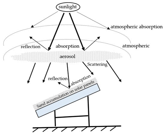
The impact of dust storms on photovoltaic (PV) output occurs in two stages: First, during the passage of a dust storm, large amounts of aerosol particles in the air block solar radiation, causing a sharp drop in the irradiance received by PV panels; second, after the dust storm has passed, the accumulation of sand on the surface of the PV panels reduces light transmittance, continuing to affect PV output [17]. Figure 1 illustrates the absorption of solar radiation by PV panels under severe dust storm conditions.

Figure 1. Schematic illustration of solar panel irradiance absorption during severe dust storms.

This paper uses the REST radiation model [18] to model solar radiation under clear-sky conditions. The formula for calculating the normal direct solar irradiance, I_n, is as follows:

$$I_n=I_{on}{T}_r{T}_g{T}_a{T}_o{T}_w$$

(1)

$$T_r=e^{[-0.0903{(m_a)}^{0.84}(1+m_a-m_a^{-1.01})]}$$

(2)

$$T_g=e^{[-0.0127m_a^{0.26}]}$$

(3)

$$m_a={\displaystyle \frac{m\cdot p}{1013}}$$

(4)

$$m=\sec \theta$$

(5)

where I_on represents the extraterrestrial irradiance (the solar constant multiplied by the correction factor for the Sun-Earth distance), with a range of 0–1367; T_r is the Rayleigh coefficient; T_g is the mixed-atmosphere transmittance; T_a is the aerosol transmittance; T_o is the ozone transmittance; T_W is the water vapor transmittance; T_r, T_g, T_a, T_o, and T_W are all dimensionless coefficients with values ranging from 0 to 1; m is the atmospheric optical mass, with values ranging from 1 to 10; p is the atmospheric pressure; and θ is the zenith angle, with values ranging from 0 to 90°.

The horizontal plane scattered irradiance I_d consists of three components:

$$I_d=D_r+D_a+D_m$$

(6)

where D_r represents the Rayleigh scattering component; D_a represents the aerosol scattering component; and D_m represents the ground-to-sky multiple scattering component.

The total horizontal solar irradiance I_g is given by:

$$I_g=I_n\cos \theta +I_d$$

(7)

Under clear-sky conditions, atmospheric aerosol concentrations remain relatively stable, and solar radiation models typically do not account for the effects of aerosols. However, during sandstorms, atmospheric aerosol thickness increases significantly, and changes in sand concentration can be reflected through changes in aerosol concentrations. Therefore, we employ a modified aerosol radiation absorption coefficient model that accounts for the effects of vertical optical depth and wavelength-dependent index variations in aerosol particles [19]:

$${\tau }_p=m_p\cdot {\tau }_{op}[1-D\alpha \sqrt{m_p-1}\sqrt[4]{{\tau }_{op}}]$$

(8)

$$D=0.1+0.035e^{[-0.95\ln ({\displaystyle \frac{m_p}{7.72}})]}$$

(9)

$$m_p={[\cos \theta +{\displaystyle \frac{a}{{(b-\theta )}^c[1+d(z-z^{*})+f{(z-z^{*})}^2]}}]}^{-1}$$

(10)

where m_p represents the relative optical path length of direct radiation; τ_op represents the effective vertical optical depth of particles, typically ranging from 0.1 to 0.3 under clear conditions and from 0.177 to 2.475 under dusty conditions; α represents the wavelength index, typically ranging from 0.94 to 1.24 under clear conditions and from 0.86 to 1.04 under dusty conditions; a = 0.4938, b = 95.4°, c = 1.5114; d = −5.96 × 10⁻⁴/m (clear weather) or −6.34 × 10⁻³/m (dust storm); f = −1.02 × 10⁻⁷/m² (clear weather) or −1.1 × 10⁻⁶/m² (dust storm); z* = 3000 m; and z is the elevation of the observation point.

$$T_a=e^{[-{\tau }_{op}^{0.873}(1+{\tau }_p-{\tau }_p^{0.7088})m^{0.9108}]}$$

(11)

Substituting into Equation (1) yields the changes in solar irradiance during severe dust storms.

When strong winds stir up dust, dust particles float in the air. As wind speeds decrease or after a dust storm has passed, the dust settles onto the photovoltaic panels due to gravity and insufficient aerodynamic force. The accumulated dust on the surface of the photovoltaic panels blocks or absorbs solar radiation, further reducing photovoltaic output. When the tilt angle of the photovoltaic panels is fixed, the light transmittance is calculated as follows:

$${\tau }_d=[1-a+a\cdot e^{b{D}^c}]{\tau }_{\mathrm{clean}}$$

(12)

where τ_clean represents the light transmittance of the photovoltaic panel under clear weather conditions; D represents the number of days of dust accumulation; and when the tilt angle of the photovoltaic panel is 40°, the empirical coefficients a, b, and c are 1.671, −0.01622, and 0.542, respectively.

Solar radiation I_j received by a dust-covered photovoltaic panel:

$$I_j=(1-{\displaystyle \frac{{\tau }_d}{100}})I_0$$

(13)

Under the influence of severe dust storms, wind turbines face multiple operational risks: First, high-speed dust flows cause abrasive damage to the blade surfaces, severely affecting the turbine’s output power; second, micron-sized dust particles penetrate the bearings of the transmission system, accelerating wear on mechanical components and damaging sealing structures; simultaneously, low-visibility operating conditions threaten the safety of operations and maintenance personnel. Therefore, this paper proposes shutting down the wind turbines for protective purposes four hours after the onset of severe dust storms, and resuming normal operation after cleaning the units using a post-disaster recovery model [20]. In actual wind turbine operations, complex failures such as blade erosion, yaw system jamming, and cooling system failure may occur in dusty environments. To focus on MES scheduling strategies, this paper employs a simplified time-based outage model. More detailed failure modeling will be addressed in future research.

2.2. A Probability Model for Power Line Failures Under Severe Dust Storm Conditions

Fine particles in dust and sand adhere to the surfaces of insulators on power transmission lines, forming a conductive layer. When air humidity is high, the conductivity of this contamination layer increases, leading to flashover, which can cause short circuits, circuit breaker trips, and even equipment damage. Dust particles accumulate on the surface of insulators, forming a conductive fouling layer that increases the equivalent salt deposition density (ESDD), thereby reducing the flashover voltage. This paper uses an exponential function to describe the relationship between the probability of flashover due to insulator fouling and the increase in dust accumulation:

$$P_{\mathrm{sand}}(t)=1-\exp \left(-{\lambda }_0{\left({\displaystyle \frac{\mathrm{ESDD}(t)}{\mathrm{ESD}{\mathrm{D}}_0}}\right)}^m\cdot \Delta t\right)$$

(14)

where λ₀ is the reference failure rate of the insulator in a clean state, taken as 1 × 10⁻³ per hour; ESDD₀ is the contamination threshold, taken as 0.1 mg/cm², a typical value; m = 2 is the nonlinear exponent; and Δt is the time step (1 h). ESDD(t) increases linearly with the accumulation time of dust, and can be approximated as ESDD(t) = min(k·t, ESDD_max), where k is the dust deposition rate, proportional to dust concentration.

This paper uses component vulnerability curves to illustrate the relationship between the intensity of extreme weather and the probability of power transmission line failures.

$$P_{\mathrm{wind}}(t)=\left\{\begin{array}{ll}0& v<V\\ \exp (0.6931{\displaystyle \frac{v(t)-V}{V}})-1& V<v<2V\\ 1& v\ge 2V\end{array}\right.$$

(15)

where P_t represents the probability of a fault occurring on the transmission line, v represents the actual wind speed, and V represents the line’s wind resistance speed, with a range of 20 m/s to 40 m/s.

Therefore, the probability of a transmission line failure is:

$$P_t(t)=1-(1-P_{\mathrm{sand}}(t))(1-P_{\mathrm{wind}}(t))$$

(16)

2.3. A Dynamic Traffic Network Model Accounting for the Impact of Severe Sandstorms

This paper employs graph theory to construct a transportation network model and provide a quantitative description of the road structure [21]. The topological structure of the road network can be described as follows:

$$\left\{\begin{array}{c}\begin{array}{l}G=(V,E,W,K)\\ V=(V_1,V_2,V_3,\dots ,V_5)\\ E=(e_{1,2},e_{2,3},\dots ,e_{4,5})\\ W=(w_{1,2},w_{2,3},\dots ,w_{4,5})\\ K=(1,2,\dots ,m)\end{array}\end{array}\right.$$

(17)

where V_i represents a road network node, and e_i,j represents an edge in the road network; therefore, G denotes the traffic network; W denotes the set of road weights; and K denotes the time scale, which divides a day into m time periods.

Traffic flow assignment is an important problem in traffic engineering and urban planning. The traditional BPR model was proposed by the U.S. Bureau of Public Roads to describe the relationship between travel time on road segments and traffic volume [22]. Although simple and easy to use, it does not account for key factors such as reduced road visibility and increased vehicle spacing caused by severe dust storms, resulting in significant prediction errors for travel times under extreme weather conditions. Therefore, this paper proposes an improved BPR model that incorporates dust storm impact factors. The improved formula is as follows:

$$t=t_0(1+\alpha {(\omega \cdot {\displaystyle \frac{Q}{C}})}^{\beta })$$

(18)

where t₀ represents the travel time under zero traffic flow; α and β are impedance factors, typically α = 0.15 and β = 4.0; Q represents the traffic flow on the road segment; C represents the road segment’s capacity; and ω is the dust coefficient, which indicates the impact of road visibility on travel time. Its value ranges from 1.0 to 1.5, with ω increasing as visibility decreases, and the specific expression is as follows:

$$\omega =1+0.5\cdot \exp \left(-{\displaystyle \frac{V_{vis}}{500}}\right)$$

(19)

where V_vis represents visibility (in meters).

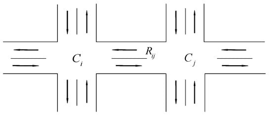
The road model is shown in Figure 2. Introducing road saturation S = Q/C, road saturation is classified into four levels based on urban traffic condition standards: 0 < S ≤ 0.6 indicates smooth traffic flow; 0.6 < S ≤ 0.8 indicates slow-moving traffic; 0.8 < S ≤ 1.0 indicates congested traffic; and 1.0 < S ≤ 2.0 indicates severe congestion. Based on the traffic conditions of the road segment, corresponding segment impedance models and node impedance models can be derived for different saturation levels [23,24].

Figure 2. Road model.

Link impedance model:

$$R_{V_{i,j}}(t)=\left\{\begin{array}{c}\begin{array}{ll}{R}_{V_{i,j}}^1(t):t_0(1+\alpha (\omega \cdot S{)}^{\beta })& \hfill 0\le S\le 1.0\hfill \\ R_{V_{i,j}}^2(t):t_0(1+\alpha (2-\omega \cdot S{)}^{\beta })& \hfill 1.0<S\le 2.0\hfill \end{array}\end{array}\right.$$

(20)

Node impedance model:

$$C_{V_i}(t)=\left\{\begin{array}{c}\begin{array}{ll}{C}_{V_i}^1(t):{\displaystyle \frac{9}{10}}\left[{\displaystyle \frac{c{(1-\omega )}^2}{2(1-\omega S)}}+{\displaystyle \frac{S^2}{2q(1-S)}}\right]& \hfill 0\le S\le 0.6\hfill \\ C_{V_i}^2(t):{\displaystyle \frac{c{(1-\omega )}^2}{2(1-\omega S)}}+{\displaystyle \frac{1.5(S-0.6)}{1-S}}S& \hfill S>0.6\hfill \end{array}\end{array}\right.$$

(21)

where c represents the signal cycle; q represents the vehicle arrival rate at the section.

By combining Equations (20) and (21) based on road saturation S, we obtain the road resistance model:

$$w_{v_i}^k(t)=\left\{\begin{array}{c}\begin{array}{ll}{R}_{V_{i,j}}^1(t)+C_{V_i}^1(t)& 0<S\le 0.6\\ R_{V_{i,j}}^1(t)+C_{V_i}^2(t)& 0.6<S\le 0.8\\ R_{V_{i,j}}^2(t)+C_{V_i}^1(t)& 0.8<S\le 1.0\\ R_{V_{i,j}}^2(t)+C_{V_i}^2(t)& 1.0<S\le 2.0\end{array}\end{array}\right.$$

(22)

The saturation level S for each road is determined based on the intensity of severe dust storms, and the road resistance w_ij for each road segment is calculated using Equation (22). This paper assumes that all roads in the traffic network G are two-way, so w_ij = w_ji. Matrix M represents the road adjacency matrix, and the assignment rules for the elements m_ij in M are shown in Equation (23), where inf indicates that there is no direct road connection between two points.

$$m_{ij}=\left\{\begin{array}{c}\begin{array}{ll}0& \hfill i=j\hfill \\ w_{ij}& \hfill ij\mathrm{is}\mathrm{an}\mathrm{edge}\mathrm{of}\mathrm{G}\hfill \\ \inf & \hfill ij\mathrm{is}\mathrm{not}\mathrm{an}\mathrm{edge}\mathrm{of}\mathrm{G}\hfill \end{array}\end{array}\right.$$

(23)

The matrix M is expressed as:

$$M=\left[\begin{array}{ccc}0& \dots & m_{1j}\\ ⋮& \ddots & ⋮\\ m_{j1}& \dots & 0\end{array}\right]$$

(24)

The matrix M reflects the level of traffic congestion through the road resistance coefficient; the higher the coefficient, the greater the congestion and the longer the travel time. Using the Floyd algorithm, we can calculate the shortest-path matrix for any two nodes in the traffic network G under severe dust storm conditions.

2.4. Monte Carlo-Based Generation of Failure Scenarios

The impact of severe dust storms on urban power and transportation systems manifests primarily in two ways. First, fine particles in the dust and strong winds cause power line failures and a significant reduction in, or even complete shutdown of, renewable energy generation. Second, reduced road visibility leads to traffic congestion and traffic accidents. To capture the randomness and time-varying nature of power line failures and road paralysis during severe sandstorms, this paper employs Monte Carlo sampling to generate failure scenarios. The sampling process converts line failure rates and road congestion rates into operational states of the urban power-transportation system, thereby enabling a resilience assessment of the system.

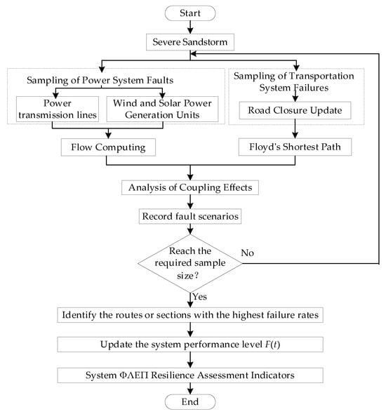
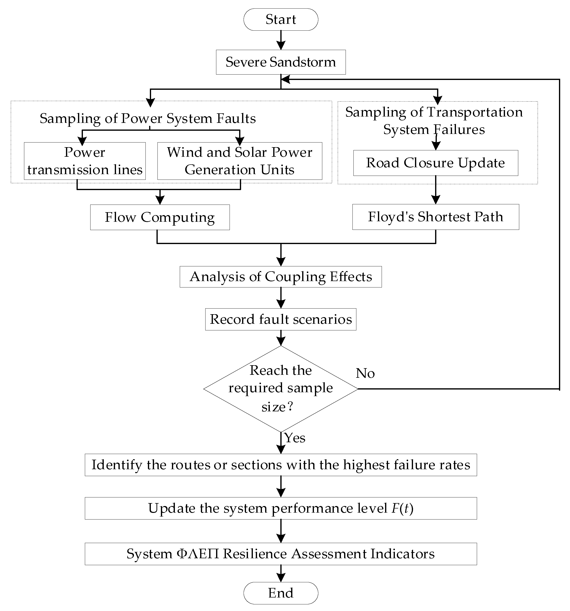
The Monte Carlo sampling process for severe sandstorms is shown in Figure 3, with the specific steps outlined below:

Figure 3. Monte Carlo Sampling Process.

Step 1: Establish a mathematical model for severe dust storms.

Step 2: Generate separate probability models for power grid failures and road network congestion under severe dust storm conditions.

Step 3: Update the power grid and road network statuses in real time and analyze their coupled effects.

Step 4: Record the failure scenarios and determine whether the required sample size has been reached. If so, terminate the sampling and identify the lines/road segments with the highest failure probability; if not, return to Step 2.

3. A Method for Assessing the Resilience of Electric–Transport Coupled Systems Considering Mobile Energy Storage

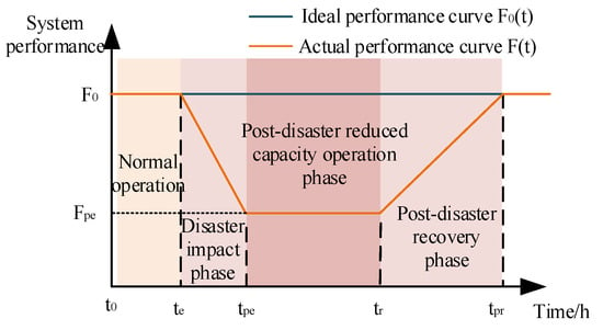
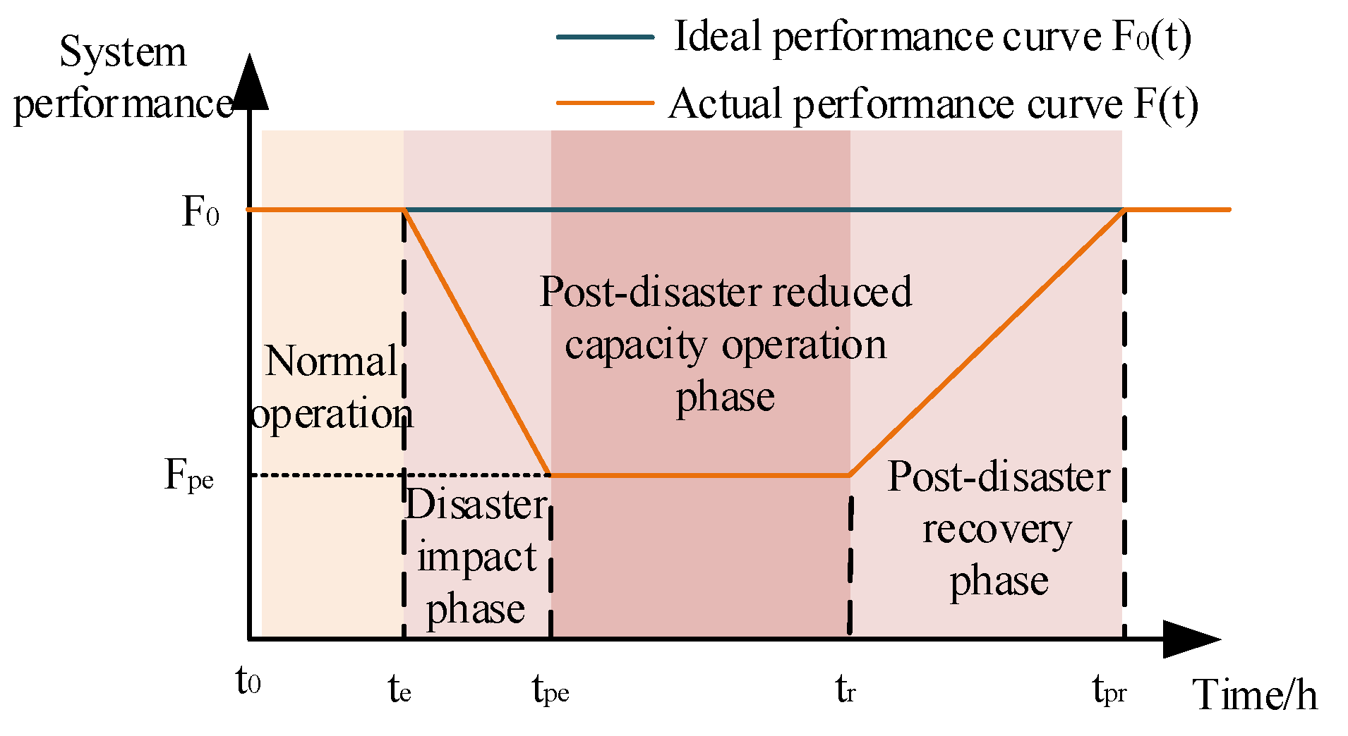
The resilience trapezoid shown in Figure 4 is used to describe changes in the system’s resilience. F(t) represents the system’s performance at time t, where t_e is the time when the system is struck by extreme weather; t_pe is the time when system performance reaches its lowest point; at time t_r, the system failure is largely repaired, and system performance begins to gradually recover; and at time t_pr, system performance is fully restored. F₀ is the ideal performance curve; under ideal conditions, system performance is 1 and remains constant. F_pe represents the actual performance curve of the system. Prior to the onset of extreme weather, the system operates normally; at time t_e, extreme weather arrives, and the system enters the disaster impact phase, during which its performance is significantly reduced due to the extreme weather; subsequently, the system enters the post-disaster derated operation phase. As the extreme weather evolves, relevant departments implement appropriate measures to maintain system performance within a stable range, preventing further decline; at time t_r, the extreme weather ends, and the system enters the post-disaster recovery phase, during which system performance gradually returns to normal levels.

Figure 4. Resilience curve.

3.1. Resilience Assessment Indicators

This paper employs the “ΦΛEΠ” index to assess the resilience of urban power-transportation systems [25,26,27,28]. The “ΦΛEΠ” index is a widely used resilience assessment metric in current research; it measures the system’s resilience level throughout the entire period of severe sandstorms by analyzing changes in system performance at different stages. The “ΦΛEΠ” resilience index is divided into two components: infrastructure resilience and operational resilience. Infrastructure resilience reflects the condition of the system’s physical facilities during extreme events, while operational resilience reflects the system’s ability to ensure normal operation. Additionally, due to differing restoration priorities, infrastructure resilience and operational resilience may not be restored simultaneously.

The specific quantitative methods for the performance indicators proposed in this paper for urban power-transportation systems are as follows:

The available MES capacity in Table 2 represents the total amount of mobile energy storage resources that can be rapidly dispatched to critical locations to provide emergency power, subject to real-time traffic conditions and grid status constraints, thereby achieving dynamic coupling between the energy storage status on the grid side and the reachability on the transportation side.

$$F_{o,c}={\displaystyle \sum _m\left(C_m(t)\cdot {\eta }_m\cdot I_t\right)}$$

(25)

where C_m(t) represents the remaining available capacity of the mth MES at time t; η_m represents the charging and discharging efficiency of the MES; and I_t represents the road connectivity and reachability index, which is a 0–1 variable.

Table 2. Performance indicators for urban power and transportation systems.

Performance Specifications	Grid-Side	Road Network Side	Coupling Node
infrastructure	Online Status of Power Transmission Lines	Road accessibility	Charging Station Availability
infrastructure resilience indicators	$F_{i,p}={\displaystyle \frac{N_{av,p}}{N_{t,p}}}$	$F_{i,t}={\displaystyle \frac{N_{av,tr}}{N_{t,tr}}}$	$F_{i,c}={\displaystyle \frac{N_{av,c}}{N_{t,c}}}$
operational facilities	Power supply reliability	Percentage of travel demand met	Available MES Capacity
operational facility resilience indicators	$F_{o,p}=ASAI$	$F_{o,tr}=\overline{T_{travel}}$	$F_{o,c}=C_{MES}$

The power restoration capability index of node j is defined as:

$$R_j=\min \left({\displaystyle \frac{F_{o,c}}{D_j}},1\right)$$

(26)

where D_j is the critical load demand at node j.

In Table 2, N_av,p, N_av,tr, and N_av,c represent the number of operational transmission lines, the number of passable roads, and the number of available charging stations, respectively; N_t,p, N_t,tr, and N_t,c represent the total number of transmission lines, the total number of roads, and the total number of charging stations, respectively;

Based on the above, the basic resilience and operational resilience indicators for the urban power-transportation system are:

$$\left\{\begin{array}{c}\begin{array}{l}{F}_i={\alpha }_i{F}_{i,p}+{\beta }_i{F}_{i,t}+{\gamma }_i{F}_{i,e}\\ F_o={\alpha }_o{F}_{o,p}+{\beta }_o{F}_{o,t}+{\gamma }_o{F}_{o,e}\end{array}\end{array}\right.$$

(27)

where α_i, α_o, β_i, β_o, γ_i and γ_o are weighting coefficients. In this paper, α_i = α_o = 0.4, β_i = β_o = 0.4, and γ_i = γ_o = 0.2.

The meaning and calculation formulas of the ΦΛEΠ toughness index are shown in Table 3.

Table 3. ΦΛEΠ resilience index.

Symbol	Meaning	Calculation Formula
		Infrastructure Resilience	Operational Resilience
Φ	system performance degradation rate	${\displaystyle \frac{F_{i,0}-F_{i,pe}}{t_{i,pe}-t_{i,e}}}$	${\displaystyle \frac{F_{o,0}-F_{o,pe}}{t_{o,pe}-t_{o,e}}}$
Λ	system performance degradation	$F_{i,0}-F_{i,pe}$	$F_{o,0}-F_{o,pe}$
E	duration of reduced-capacity operation	$t_{i,r}-t_{i,pe}$	$t_{o,r}-t_{o,pe}$
Π	system recovery rate	${\displaystyle \frac{F_{i,0}-F_{i,pe}}{t_{i,pe}-t_{i,r}}}$	${\displaystyle \frac{F_{o,0}-F_{o,pe}}{t_{o,pe}-t_{o,r}}}$
Area	system Performance	${\displaystyle {\int }_{t_{i,e}}^{t_{i,pr}}{F}_i(t)}dt$	${\displaystyle {\int }_{t_{o,e}}^{t_{o,pr}}{F}_o(t)}dt$

In the calculation formula, F₀ represents the system’s normal operating performance, with a standard normal value of 1. F_pe represents the minimum performance level of the system after it has been hit by a severe sandstorm, t_e represents the time when the system is struck by the severe sandstorm, t_pe represents the time when the system’s performance reaches its lowest point, t_r represents the time when the system’s performance begins to recover, and t_pr represents the time when the system’s performance returns to normal.

3.2. Coordinated Architecture for Urban Power and Transportation Systems

The enhancement of urban power-transportation system resilience discussed in this paper does not involve constructing a new, independent physical network, but rather establishing cross-system collaborative recovery capabilities through the dynamic scheduling of MES based on the existing fixed topology. Specifically, when a power grid node loses power due to a fault and lacks a local power source, MES can transport energy from a nearby powered node to the power-deficient node, enabling temporary energy transfer; when a section of the road network is congested due to sandstorms, MES can select alternative routes or utilize emergency contraflow lanes. This mechanism of “Mobile Energy Storage as a Dispatchable Resource” effectively overlays a resilient network onto the fixed physical topology. This network does not alter the original topological structure but provides temporary recovery capabilities through the spatiotemporal transfer of MES, thereby enhancing the system’s adaptability and resilience in the face of node failures.

To characterize the damage status of urban power-transportation systems under extreme weather conditions, this paper builds upon the work in [29] by incorporating mobile energy storage (MES) into emergency response efforts. Mobile energy storage enables bidirectional power flow through charging stations: during normal grid operations, MES units charge via the charging stations; when the grid loses power, MES units can supply power back to the grid (V2G) through the charging stations to support critical loads. Meanwhile, the connection status of MES units is dynamically updated based on real-time damage information.

$$\left\{\begin{array}{c}\begin{array}{l}{y}_j^{DN}=y_m^{CS}=y_l^{TN}\\ y_c^{MES}=y_m^{CS}\cap (1-y_j^{DN})\end{array}\end{array}\right.$$

(28)

where y_j^DN represents the power supply status of grid node j; y_m^CS represents the availability status of charging station m; y_l^TN represents the passability status of road p; and y_c^MES represents the connection status of the cth MES. All of these are binary variables.

When grid equipment fails—such as when a transmission line or utility pole collapses—obstacles block the lanes, reducing road capacity. The expression for the remaining road capacity is:

$$C_a^{\tau }=C_a^0(1-\min \left\{1,{\displaystyle \sum _l{\tau }_{l,a}\cdot y_l^{TP}}\right\})$$

(29)

where C_a⁰ represents the road capacity under normal conditions, y_l^TP = 1 indicates that an obstacle is occupying the lane, and τ_l,a ∈ [0, 1] denotes the proportion of capacity loss for road a.

In actual disasters, damage to the transportation network also affects the rate of power grid restoration: disruptions to key roads cause emergency repair vehicles to arrive late at the site of the power grid failure, thereby affecting the power grid repair rate:

$${\mu }_{l,t}={\mu }_l^0\cdot {\delta }_{l,t}$$

(30)

where μ_l⁰ represents the ideal repair rate; δ_l,t is a binary variable, where δ_l,t = 0 indicates that the emergency repair vehicle cannot reach the failure point.

To enhance the symmetry of the bidirectional coupling between the power grid and transportation, this paper introduces a model that accounts for the impact of power outages on traffic signals and EV charging behavior. Let the operational state of the traffic signal at node i be denoted by the binary variable s_i,t, which is determined by the power supply status of the corresponding grid node:

$$s_{i,t}=y_{j(i),t}^{DN}$$

(31)

where j(i) denotes the number of the grid node coupled to traffic node i. When the traffic signal fails, the intersection’s traffic capacity decreases, and the effective capacity of road a is adjusted as follows:

$$C_{a,t}^{eff}=C_a^0\cdot \left(0.6+0.4s_{i(a),t}\right)$$

(32)

where i(a) denotes the upstream intersection node on road a.

For EV charging behavior, when charging station c becomes unavailable due to a power outage (z_c,t = 0), EVs originally scheduled to charge there will divert to the nearest available charging station c′, resulting in additional travel time:

$$\Delta T_{ev}={\displaystyle \sum _{c\in \Omega }(1-z_{c,t})\cdot \frac{d_{c\to c^{\prime }}}{v_{\mathrm{avg}}}}$$

(33)

This time increment is reflected in the dynamic updates to the traffic resistance matrix via the Floyd algorithm.

4. A Multi-Stage Resilience Enhancement Strategy Using Mobile Energy Storage

Mobile energy storage is characterized by its ease of dispatch and widespread application in urban areas [30]. In the problem of coordinated dispatch of mobile energy storage for resilience enhancement, the power grid must determine the priority of power restoration, while the transportation network must determine the optimal routes for mobile energy storage. The three-stage resilience enhancement strategy proposed in this paper corresponds to the time intervals t_o − t_e, t_e − t_s, and t_s − t_pr on the resilience curve.

Based on the progression of extreme weather events and the characteristics of system resilience, the resilience enhancement strategy is divided into three phases: pre-disaster pre-deployment, in-disaster response, and post-disaster recovery. The mobile energy storage units considered in this paper can be charged at charging stations and can also discharge power to the grid (V2G) to provide short-term power to critical loads or nodes, and their operations are influenced by traffic network connectivity. The objectives are to minimize the total expected cost, minimize the power restoration time for the grid, and minimize the expected travel time on the road network. The objective function is as follows:

$$\min (F_1,F_2,F_3)$$

(34)

$$\left\{\begin{array}{c}\begin{array}{l}{F}_1=C_{pre}+{\displaystyle \sum _s{p}_s(C_{res}+C_{recover})}\\ F_2={\displaystyle \sum _s{p}_s{\displaystyle \sum _i{\omega }_i(T_{i,s}^{res}+T_{i,s}^{recover})}}\\ F_3={\displaystyle \sum _s{p}_s{\displaystyle \sum _k{q}_k({\tau }_{i,s}^{res}+{\tau }_{i,s}^{recover})}}\end{array}\end{array}\right.$$

(35)

where F₁ represents the total expected cost, F₂ represents the weighted power restoration time, and F₃ represents the expected travel time in the road network. C_pre, C_res, and C_recover represent the pre-disaster pre-scheduling cost, in-disaster response cost, and post-disaster recovery cost of the urban power-transportation system, respectively; T_res and T_recover represent the recovery time during the grid response phase and the recovery phase, respectively; ω_i is the importance weight of grid node i; τ_res and τ_recover are the shortest path travel times during the road network response phase and recovery phase, respectively; and q_k is the weight of the traffic demand at node k.

Since the three objectives have different units, this paper first normalizes the three objective functions:

$$x_{\mathrm{nor}}={\displaystyle \frac{x-x_{\min }}{x_{\max }-x_{\min }}}$$

(36)

where x_nor represents the normalized data; x represents the raw data; and x_min and x_max represent the minimum and maximum values of the raw data, respectively.

4.1. Pre-Disaster Preparation Phase

This paper utilizes the predictability of severe dust storms to consider extreme wind and solar power output scenarios, generates typical failure scenarios, and establishes a pre-scheduling model. Pre-scheduling aims to deploy mobile energy storage to optimal locations prior to a disaster so that, when extreme weather strikes, the mobile energy storage can respond rapidly and participate in load restoration and road section repairs. The constraints include pre-deployment cost constraints, mobile energy storage resource constraints, traffic flow balancing constraints, MES operational constraints, distribution network radial topology constraints, and renewable energy output constraints.

(1)

Pre-deployment cost constraints

$$C_{pre}={\displaystyle \sum _e{C}_e{x}_e+{\displaystyle \sum _m{C}_{\mathrm{MES}}\cdot N_{\mathrm{MES}}\le B_{pre}}}$$

(37)

where C_e represents the reinforcement cost of system component e; x_e is a binary variable, i.e., the decision variable indicating whether to reinforce component e; C_MES represents the unit configuration cost of MES; and N_MES represents the number of MES units configured. B_pre represents the upper limit of the pre-disaster investment budget.

(2)

Mobile Energy Storage Resource Constraints. The amount of mobile energy storage resources available prior to a disaster is limited. Assuming that all mobile energy storage devices have identical parameters, a single task point may be served by multiple mobile energy storage units, but a single mobile energy storage unit can serve only one task point.

$${\displaystyle \sum _{i\in \Omega }{\alpha }_{i,0}^{pr}\le N_{\max }^{pr}}$$

(38)

where N_max represents the upper limit on the number of mobile energy storage units during the preliminary deployment phase. α is a variable ranging from 0 to 1; if a mobile energy storage unit is deployed at a node, then α = 1.

(3)

MES operational constraints

$$0\le P_{j,t}^c\le {\alpha }_{j,t}^c{P}_{j,\max }^c{\alpha }_{j,t}^c\in \left\{0,1\right\}$$

(39)

$$0\le P_{j,t}^d\le {\alpha }_{j,t}^d{P}_{j,\max }^d{\alpha }_{j,t}^d\in \left\{0,1\right\}$$

(40)

$${\alpha }_{j,t}^c+{\alpha }_{j,t}^d\le 1$$

(41)

$$SO{C}_{\min }\le SO{C}_{j,t}^{\mathrm{MES}}\le SO{C}_{\max }$$

(42)

$$SO{C}_{j,t}^{\mathrm{MES}}=SO{C}_{j,0}^{\mathrm{MES}}+Q_{j,\mathrm{MES}}^{-1}(P_{j,t}^c-P_{j,t}^d)\Delta t$$

(43)

$$SO{C}_{j,t}^{\mathrm{MES}}-{\displaystyle \frac{d_j(t)\cdot \epsilon }{Q_{j,\mathrm{MES}}}}\ge SO{C}_{\min }^{\mathrm{travel}}$$

(44)

where P^c_j,t and P^d_j,t represent the power of the jth MES during charging and discharging at time t, respectively; α^c_j,t and α^d_j,t are the state variables for the jth MES during charging and discharging at time t, with a value of 1 indicating that the MES is in the charging or discharging state; SOC^MES_j,t and SOC^MES_j,0 represent the state of charge of the jth MES at time t and at the initial time, respectively; Q_j,MES is the rated battery capacity of the jth MES; Δt denotes the duration during which the MES participates in discharging; d_j(t) is the distance traveled by the jth MES during time interval t; and ε is the energy consumption per unit distance of the MES, a constant typically set to 0.2 kWh/km.

The total discharge power W_d(t) of the MES at discharge station d at time t is expressed as:

$$W_d(t)={\displaystyle \sum _{j=1}^N(k_{j,t}}{P}_{j,t}^d)d\in D$$

(45)

where D represents the set of all discharge stations; N is the number of MES units participating in discharge at station d; and k_j,t denotes the discharge status of the jth MES unit at time t, which is 1 if discharging and 0 otherwise.

Given that MES discharge behavior affects battery life, their discharge capacity is expressed in terms of remaining discharge capacity as follows:

$$Q_{j,t}^d=\left\{\begin{array}{l}0,SO{C}_{j,t}^d\le 0.2\\ \left(SO{C}_{j,t}^d-0.2\right)\times Q_{j,\mathrm{EV}},SO{C}_{j,t}^d>0.2\end{array}\right.$$

(46)

where Q^d_j,t represents the remaining discharge capacity of the jth MES at discharge station d at time t; SOC^d_j,t represents the state of charge of the jth MES’s battery prior to discharge at discharge station d at time t.

(4)

Traffic flow balance constraint. This ensures that traffic flow is conserved in the traffic network under disaster scenario k.

$${\displaystyle \sum _{a\in A^{in}}{f}_{a,k}+q_{i,k}={\displaystyle \sum _{a\in A^{out}}{f}_{a,k}}}$$

(47)

where q_i,k represents the traffic demand at node i.

(5)

Distribution network radial topology constraints. To account for both island merging and power-deficient islands, an improved single-commodity flow method is employed to ensure that the distribution network satisfies the radial topology requirements during the restoration process.

$${\displaystyle \sum _{ij\in {\Omega }_B}{\alpha }_{ij}=N_B-{\displaystyle \sum _{i\in {\Omega }_N}{S}_i^{VS}}}$$

(48)

$${\displaystyle \sum _{j\in \delta (i)}{F}_{ij}-{\displaystyle \sum _{k\in \gamma (i)}{F}_{ki}=F_i^{VS}-1}}$$

(49)

$$-M_1{S}_i^{VS}\le F_i^{VS}\le M_1{S}_i^{VS}$$

(50)

$$-M_1{\alpha }_{ij}\le F_{ij}\le M_1$$

(51)

where Ω denotes the set of branches; N_B denotes the total number of nodes; δ(i) and γ(i) denote the sets of child and parent nodes of node i, respectively; F_ij denotes the virtual power flow in branch i; F_i^VS denotes the virtual power generated by node i; and M₁ denotes a very large number, taken as 10⁶.

(6)

Renewable energy output constraints. The output of distributed power sources at each node should not exceed their output limits. Assuming that, prior to the disaster, mobile energy storage systems and electric vehicles connected to charging stations were fully charged, the upper limit of their discharge power is taken as their output limit.

$$-{\displaystyle \sum {\alpha }_i^{DG}{P}_{i,\max }^{DG}}\le P_i^{DG}\le {\displaystyle \sum {\alpha }_i^{DG}{P}_{i,\max }^{DG}}$$

(52)

$$-{\displaystyle \sum {\alpha }_i^{DG}{Q}_{i,\max }^{DG}}\le Q_i^{DG}\le {\displaystyle \sum {\alpha }_i^{DG}{Q}_{i,\max }^{DG}}$$

(53)

4.2. Strategies for Enhancing Resilience During the Pre-Disaster Planning Phase

During severe dust storms, renewable energy output drops rapidly, grid load fluctuates significantly, and the failure rate of the road network increases. To prevent the system’s resilience from dropping to a minimum, emergency strategies are implemented to ensure normal power supply at critical grid nodes.

The constraints are as follows: load shedding constraint, road network reverse flow constraint, and distribution network power flow constraint.

(1)

Grid load shedding constraint. Limits the amount of load shed within a single time interval.

$$0\le \Delta P_{d,t}\le P_{d,t}^{\max },d\in D$$

(54)

$$P_{d,t-1}\le P_{d,t}\le P_{d,t}^{\max }$$

(55)

where ΔP_j,t represents the load shedding at node j during time step t (kW), and P_j,t represents the actual power supplied at node j during time step t (kW).

(2)

Reverse-direction traffic on the road network. To ensure that MES vehicles can reach key nodes, traffic may travel in the opposite direction when necessary.

$$C_a=C_a^0(1-{\lambda }_A)+C_{a\prime }^0{\lambda }_{a\prime }$$

(56)

$${\lambda }_a+{\lambda }_{a\prime }\le 1$$

(57)

$${\displaystyle \sum {\lambda }_a\le N_{TN}}$$

(58)

where λ_a is the decision variable (0–1) for vehicle traffic traveling in the opposite direction.

(3)

Power flow constraints. This paper uses the DistFlow model to impose constraints on power flows in the distribution network.

$${\displaystyle \sum (P_{ij}-{\left|I_{ij}\right|}^2{r}_{ij})+P_j={\displaystyle \sum P_{jk}}}$$

(59)

$${\displaystyle \sum (Q_{ij}-{\left|I_{ij}\right|}^2{x}_{ij})+Q_j={\displaystyle \sum Q_{jk}}}$$

(60)

$$U_i(t)-U_j(t)\ge -M_{ij}(1-{\mu }_{ij})+2(r_{ij}{P}_{ij}(t)+x_{ij}{Q}_{ij}(t)),\forall (i,j)\in E_L$$

(61)

$$U_i(t)-U_j(t)\le M_{ij}(1-{\mu }_{ij})+2(r_{ij}{P}_{ij}(t)+x_{ij}{Q}_{ij}(t)),\forall (i,j)\in E_L$$

(62)

where μ_ij is a binary variable used to represent the line status; it equals 0 when the line is out of service.

(4)

MES reverse power injection constraint.

$$0\le P_{w,t}^{\mathrm{V}2\mathrm{G}}\le P_{\max }^{\mathrm{V}2\mathrm{G}}\cdot y^{\mathrm{MES}}$$

(63)

where P^V2G represents the power supplied by the MES to the grid, and P^V2G_max represents the maximum power that the MES can supply to the grid. Reverse power flow is permitted only when the MES is physically connected and the charging station is operating normally.

(5)

Charging station operational constraints.

$${\displaystyle \sum _k{p}_{kt}\le {\displaystyle \sum _c{P}_c^{\max }\cdot g_{ct}}}$$

(64)

$${\displaystyle \sum _m{z}_{m,c}(t)\le N_c^{\max },\forall c,t}$$

(65)

where p_kt represents the power injected into the grid by the MES; P^max denotes the maximum V2G power capacity of the charging station; and g_ct is a binary variable indicating the connectivity status between charging station c and the grid at time t. z_m,c(t) denote a binary variable indicating whether the mth MES is connected to charging station c at time t; let N_c^max denote the maximum number of MESs that charging station c can serve simultaneously.

4.3. Strategies for Enhancing Resilience During the Disaster Response Phase

The post-disaster recovery phase involves effectively repairing faulty components and resolving traffic congestion under specific failure scenarios to restore system resilience as quickly as possible.

(1)

Maintenance queue constraints.

$${\displaystyle \sum _{t\in R_t}(1-\delta )\le N_{re}}$$

(66)

where R_t represents the set of system components at time step t, and N_re represents the upper limit on the number of maintenance teams.

(2)

MES mobile location constraints.

$${\displaystyle \sum _i{x}_i^m\le x_d^m}$$

(67)

$${\displaystyle \sum _d{\displaystyle \sum _m{x}_{d,t}^m}}\le 1$$

(68)

$$x_{d,t}^m+x_{i,t+\tau }^m\le 1$$

(69)

where x_d^m, t is a 0–1 variable representing the mth MES access node d at time step t; x^m_i,t+τ is a binary variable indicating whether the mth MES is connected to node i after a time interval of τ.

5. NSGA-II Algorithm

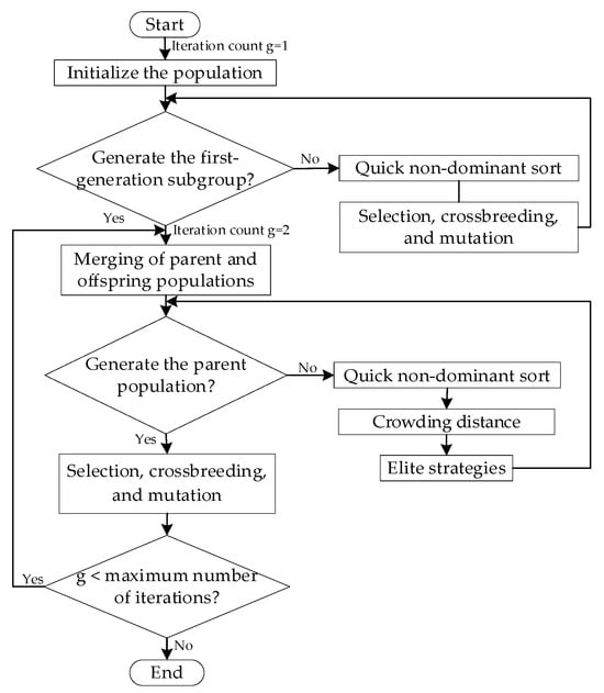
When addressing complex multi-objective optimization problems, the objectives are often conflicting, and there is no single optimal solution; rather, there is a set of trade-off solutions known as the Pareto-optimal solution set. This paper employs the NSGA-II algorithm [31,32] to solve the proposed model. The core of the NSGA-II algorithm lies in its use of non-dominance sorting and the crowding mechanism to ensure convergence while maintaining a uniform distribution of the solution set. First, crossover and mutation operations are performed on the parent population P(t) of size N to generate a child population Q(t) of the same size. The parent and child populations are then merged to form a new population R(t) of size 2N. Subsequently, R(t) is sorted by non-dominance, and an elite strategy is used to select the N best individuals from it to form the new parent population P(t + 1). This process is repeated until the iteration termination conditions are met, and the optimal solution set composed of the parent population is finally output.

5.1. Individual Coding and Parameter Settings

This paper employs a hybrid encoding method to map optimization variables onto the chromosomes of NSGA-II individuals, with the specific structure as follows:

(1)

Pre-layout encoding. The first N_MES bits are encoded as integers, with each bit representing the node number of a MES in the pre-layout. The range of node numbers is the set of coupling nodes {1, 2, …, 9}. If N_MES < 9, unused node numbers are omitted.

(2)

In-disaster movement path encoding. The middle segment uses variable-length encoding to record the movement paths (sequence of nodes) of each MES in chronological order. The path length of each MES does not exceed the preset maximum value L_max = 5; any remaining space is padded with zeros.

(3)

Maintenance Team Scheduling Encoding. The trailing segment is a permutation encoding of the maintenance team’s task sequence. Let R denote the number of components to be repaired; the encoding is a permutation of {1, 2, …, R}, representing the component numbers processed sequentially by the maintenance team.

The algorithm parameters are set as follows: population size N = 200, maximum number of iterations G = 300, crossover probability P_c = 0.9, and mutation probability P_m = 0.1. Constraint handling employs a feasible-solution-first strategy: individuals that violate hard constraints such as node voltage, SOC safety limits, and power balance are subject to a penalty proportional to the severity of the violation; during non-dominance sorting, feasible solutions take precedence over infeasible ones. The termination criterion is reaching the maximum number of iterations, or when the rate of change in the Pareto front volume is less than 10⁻⁴ for 50 consecutive generations.

5.2. Quick Non-Dominant Sort

For each individual i in the population, set two parameters: the dominance count ni (i.e., the number of individuals that dominate individual i) and the dominated set S_i (i.e., the set of individuals dominated by individual i). Place all individuals with n_i = 0 into the first non-dominant layer Z₁. Then, for each individual p in Z₁, for each individual q in p’s S_p, set n_q = n_q − 1; if n_q = 0, place q into the next non-dominant layer Z₂. Repeat this process until all individuals have been assigned to layers.

5.3. Crowding Distance

Individuals within the same non-dominant layer are sorted by the values of each objective function, and the crowding index i_d is defined as the sum of the absolute distances between an individual and its neighbors across all objectives, normalized as follows:

$$i_d={\displaystyle \frac{{\displaystyle \sum _{l=1}^m\left(\left|f_l^{i+1}-f_l^{i-1}\right|\right)}}{f_l^{\max }-f_l^{\min }}}$$

(70)

where i_d represents the crowding distance of individual i; f_lⁱ represents the value of the first objective function for individual i; f_l^max represents the maximum value of the first objective function; and f_l^min represents the minimum value of the first objective function.

5.4. NSGA-II Algorithm Flowchart

In summary, the NSGA-II algorithm achieves this through the synergistic interaction of non-dominance sorting, crowding degree calculation, and an elite selection mechanism. Its complete workflow is shown in Figure 5:

Figure 5. NSGA-II algorithm flowchart.

6. Case Study Analysis

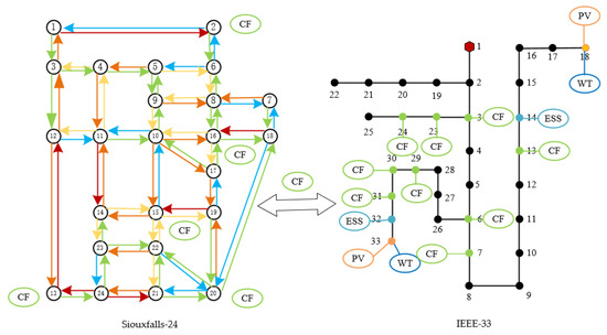
To validate the effectiveness of the proposed model and method, this paper constructs a coupled system using the IEEE 33-node distribution network test system and the 24-node Sioux Falls network, the topology diagram is shown in Figure 6. Nine charging stations were selected as coupling nodes; the geographical correspondence between distribution network nodes and road traffic nodes is shown in Table 4. Simulation analysis was performed using the MATLAB R2018b platform. Distribution network parameters were set according to Reference [33]. For the grid side, nodes with higher loads were selected for coupling with road network nodes with higher traffic volumes, and each grid node was coupled with only one road network node. In the case study, a severe sandstorm begins at 8:00 and lasts for 4 h. The Sioux Falls transportation network was modeled using a standard open dataset that includes 24 nodes and 76 links [34]. The average vehicle speeds under normal weather conditions and severe dust storm conditions are 60 km/h and 30 km/h, respectively. Mobile energy storage units have sufficient time to be deployed at pre-designated nodes prior to the disaster. The maximum number of mobile energy storage units available for pre-scheduling is 5, with each unit having a capacity of 500 kWh.

Figure 6. Urban power and transportation system topology diagram.

Table 4. Correspondence table for coupling nodes between power distribution networks and transportation networks.

Power Grid Node Number	Road Network Node Number	Coupling Node Number
3	16	1
6	20	2
7	22	3
13	2	4
23	10	5
24	11	6
29	17	7
30	15	8
31	13	9

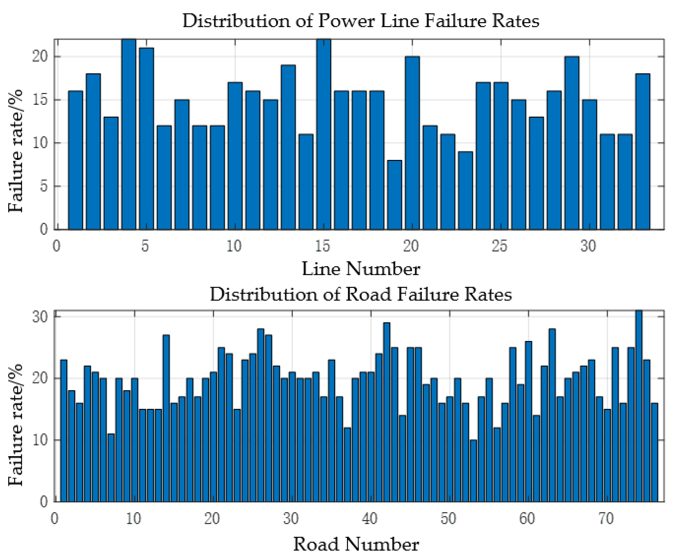
A Monte Carlo sampling method is used to generate a failure probability model for the urban power-transportation system. The line with the highest failure rate is selected as the initial state of the system following damage caused by a severe dust storm.

Based on the failure probability model shown in Figure 7, failure scenarios were generated using 500, 1000, 2000, and 5000 samples, respectively, to calculate the average system resilience under the original design. The results show that when the number of samples increases from 1000 to 2000, the change in system resilience is less than 1%; when it increases from 2000 to 5000, the change is less than 0.5%. Therefore, the 2000 samples used in this paper are sufficient to ensure the stability of the results.

Figure 7. Probabilistic failures in urban power and transportation systems.

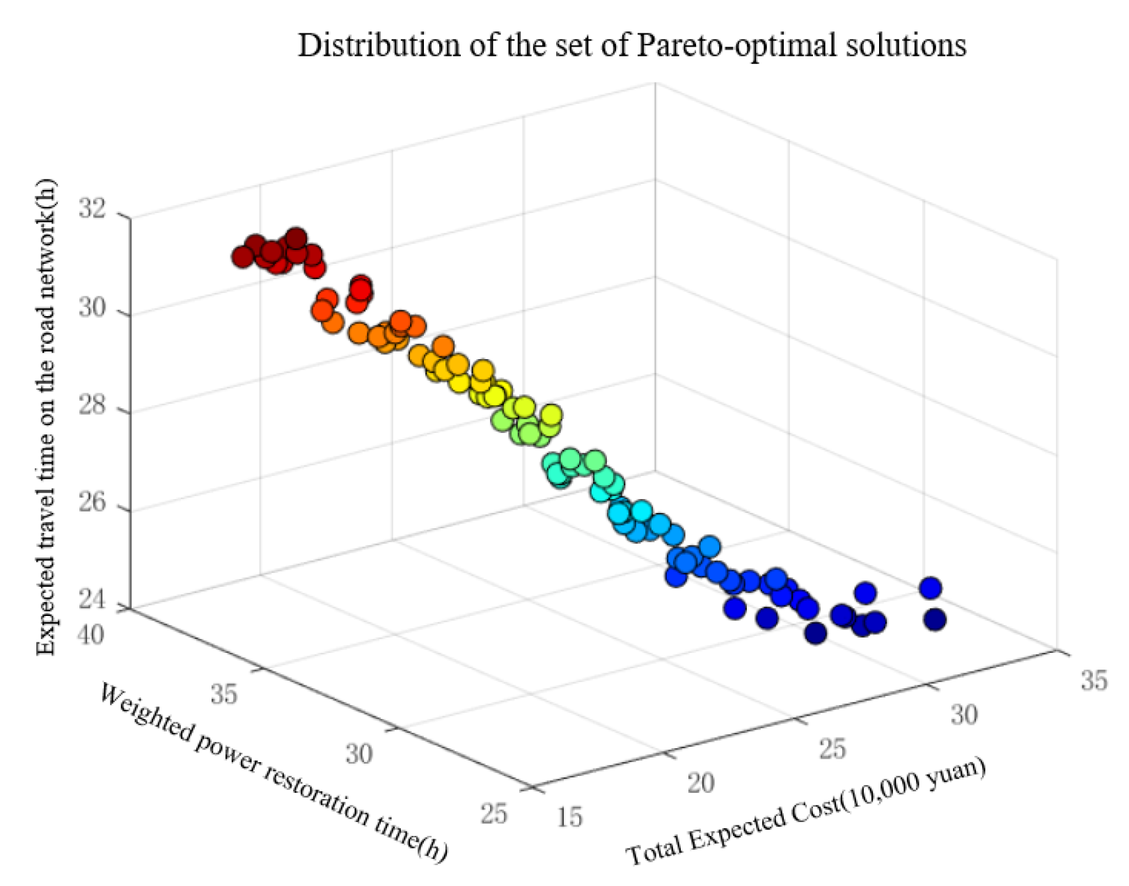
The NSGA-II algorithm was used to solve the three-objective optimization problem, yielding a set of Pareto-optimal solutions for each objective function; three representative optimal solutions were selected from this set for in-depth analysis.

6.1. Pre-Disaster Planning

The core task of the pre-disaster pre-deployment phase is to enhance the system’s initial resilience by relocating mobile energy storage units to vulnerable points in the system before severe dust storms strike. The results of the MES pre-deployment for three typical scenarios are shown in Table 5, with one MES unit deployed at each coupling node:

Table 5. MES pre-assigned locations.

Typical Scenarios	MES Configuration Nodes (Grid Side → Road Network Side)
Minimum-cost solution	3 → 16, 13 → 2, 31 → 13
Quickest recovery solution	3 → 16, 6 → 20, 7 → 22, 13 → 2, 23 → 10
Optimal traversal solution	3 → 16, 24 → 11, 30 → 15, 31 → 13

The preliminary layout plan for the minimum-cost solution embodies the principle of prioritizing economic efficiency, selecting three MES units to be centrally deployed at critical nodes of the power grid and key hubs of the road network. Geographically, this plan forms a triangular support structure, covering critical load areas with minimal resources. The fastest power grid restoration solution adopts a comprehensive defense strategy, deploying all five MES units to form a distributed MES network. This ensures rapid restoration capabilities for backbone lines and continuous power supply to critical loads, creating multi-source support to prevent system collapse caused by single-point failures. The optimal road network connectivity solution’s preliminary layout deploys four MES units, prioritizing the repair of failed roads to ensure road connectivity and accessibility to failure points.

6.2. Response Phase During a Disaster

Immediately after a disaster occurs, emergency measures are implemented to mitigate the rapid decline in system performance. During this phase, based on the initial MES locations specified in the pre-deployment plan, the Floyd algorithm is used to calculate the shortest path for the MES to move to the failed node in response to the system failure. The MES movement paths are shown in the table below (Table 6):

Table 6. MES dynamic scheduling process.

Solution	1	2	3	4	5
Original proposal	×	×	×	×	×
Minimum-cost solution	3 → 8 → 9	13 → 12 → 11	×	×	×
Quickest recovery solution	3 → 4 → 5	6 → 7 → 8	×	13 → 15	23 → 25
Optimal traversal solution	×	3 → 1 → 2	11 → 12	×	13 → 24 → 21 → 20

In the table, an “×” indicates that the mobile energy storage system has not been deployed in the system or will not be moved during the disaster response phase.

6.3. Post-Disaster Recovery Phase

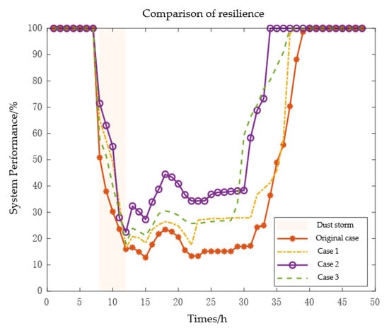
Following the end of the severe dust storm, the resilience of the urban power-transportation system was restored through the coordinated use of various resources. Figure 8 shown the three-dimensional distribution of the Pareto front obtained from the NSGA-II runs Figure 9 shows the comprehensive resilience change curves for each scenario within 48 h before and after the disaster. It can be seen that the severe dust storm caused a massive impact on the system within 4 h of its onset, resulting in a sharp decline in system resilience. However, because different pre-disaster layout scenarios were already in place, the lowest points in system performance were improved to varying degrees compared to the baseline scenario. All three optimized scenarios demonstrated higher resilience levels than the baseline scenario across all three phases. Among them, the “fastest grid recovery” scenario exhibited the highest resilience during the disaster and the fastest recovery speed, with a minimum resilience value of 22.47%—a 40.4% improvement over the baseline scenario’s 16%.

Figure 8. Distribution of the set of Pareto-optimal solutions.

Figure 9. Comparison of resilience in urban power and transportation systems.

Table 7 shows the average resilience, system recovery time, and total costs from the onset of the disaster through to full system restoration.

Table 7. Comparison of options.

Solution	Average Resilience	Recovery Time/h	Total Cost/10,000 yuan
Original proposal	52.62	40	26.78
Minimum-cost solution	58.75	38	15.68
Quickest recovery solution	68.70	26	34.35
Optimal traversal solution	64.25	37	19.87

Compared to the baseline scenario, the three optimization strategies improved the resilience of the urban power-transportation system by 11.4%, 30.56%, and 22.1%, respectively, with the fastest grid recovery solution yielding the highest average system resilience. Recovery times were reduced by 2 h, 14 h, and 3 h, respectively. In terms of total cost, the Minimum Cost Solution reduces costs by 41.45% compared to the original plan, the Fastest Recovery Solution increases costs by 28.27%, and the Optimal Throughput Solution reduces costs by 25.80%. Overall, while the fastest grid restoration solution offers the highest system resilience, it also incurs higher costs. Conversely, the minimum-cost solution incurs the lowest costs but results in the slowest system recovery rate.

6.4. Analysis of System Resilience Under Different Dust Storm Parameters

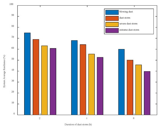
To verify the applicability of the method proposed in this paper under different durations and intensities of dust storms, this section sets three durations (2 h, 4 h, and 6 h) and four dust storm levels (dust, sandstorm, severe sandstorm, and extreme sandstorm) to calculate the average system resilience under the original approach. As shown in Figure 10, the resilience of the coupled system decreases as the severity and duration of the disaster increase. The model exhibits good physical consistency, indicating that the method proposed in this paper is applicable to sandstorms of varying intensities and durations.

Figure 10. System-wide average resilience under varying durations and intensities of dust storms.

7. Summary

To address the research on resilience assessment and enhancement strategies for urban power-transportation systems, this paper proposes a resilience enhancement strategy that incorporates mobile energy storage. A three-stage optimization model—pre-disaster planning, in-disaster response, and post-disaster recovery—was established. Case studies validated the effectiveness of the proposed model, and the conclusions are as follows:

(1)

To address the uncertainties in renewable energy output and road network travel times under severe sandstorm conditions, a failure probability model for urban power-transportation systems in severe sandstorm environments was established, capable of accurately characterizing system failures under extreme weather conditions.

(2)

A ΦΛEΠ resilience index suitable for urban power-transportation systems was proposed. Based on infrastructure resilience and operational resilience, a multidimensional resilience assessment index was constructed for the power side, transportation side, and coupling nodes, providing theoretical support for system resilience evaluation.

(3)

A multi-stage resilience enhancement strategy incorporating mobile energy storage was proposed. Through coordinated optimization across three phases—pre-disaster pre-deployment, in-disaster response, and post-disaster recovery—a Pareto-optimal solution set was obtained using the NSGA-II algorithm, and three typical scenarios were analyzed. The results of the case studies indicate that the three typical optimal solutions perform excellently in their respective target domains: the minimum-cost solution reduces the total system recovery cost by 41.25%, the fastest grid recovery solution shortens the system recovery time by 35%, and the optimal road network solution improves system traffic efficiency by 22%.

(4)

This study makes a vital contribution to sustainable development by enhancing the resilience of coupled urban power-transportation systems against climate-induced extreme weather (aligning with SDG 11: Sustainable Cities and Communities). By integrating mobile energy storage (MES), the proposed framework not only mitigates socioeconomic disruptions during severe dust storms but also facilitates the stabilization and utilization of renewable energy under volatile conditions (aligning with SDG 7: Affordable and Clean Energy). Consequently, this research provides a scientific decision-making pathway for constructing low-carbon, secure, and climate-resilient future smart cities, offering profound ecological and economic benefits for sustainable infrastructure.

The dust optical and dust accumulation models employed in this paper are taken directly from previous studies [17,18,19,20], which have already been validated against experimental or field data. Consequently, we did not perform an independent calibration using real dust storm data, and we acknowledge this as a limitation of the current work. Future research will incorporate measured power and meteorological data from the dust storm events to further validate these models. Additionally, this paper does not account for the cycle life degradation or thermal constraints of MES batteries; more detailed battery degradation models will be introduced in future work. This paper assumes that dispatch instructions can be transmitted in real time during severe dust storm events. In practice, severe dust storms may cause communication disruptions; however, this paper does not currently account for communication failures, which constitutes an idealized assumption. Future research will incorporate a vulnerability model for communication networks.

References

- Available online: https://www.gov.cn/zhengce/zhengceku/2022-04/06/content_5683595.htm (accessed on 16 June 2026).
- Available online: https://www.ndrc.gov.cn/xxgk/zcfb/ghwb/202103/t20210323_1270124_ext.html (accessed on 16 June 2026).
- Ji, T.; Yao, Y.; Huang, X.; Zhu, Y.; Deng, S.; Yu, S.; Liao, H. Progress and future development trend of urban transportation resilience research. Prog. Geogr. 2023, 42, 1012–1024. [Google Scholar] [CrossRef] [Scilit]
- Tang, Y.; Chen, X. Strong Winds and Dust Storm Affect Travel on 106 Road Sections. CCTV News. 2025. Available online: http://www.bjnews.com.cn/detail/1744423886129942.html (accessed on 16 June 2026).
- Ju, G.; Wang, J.; Cui, C.; Zhang, P.; Si, Y.; Fan, X.; Qiu, W. Impact of Extreme Weather Events on New Energy Power Generation and Power Grid Operation. Smart Power 2022, 50, 77–83. [Google Scholar] [CrossRef]
- Hossain, E.; Roy, S.; Mohammad, N.; Nawar, N.; Dipta, D.R. Metrics and enhancement strategies for grid resilience and reliability during natural disasters. Appl. Energy 2021, 290, 116709. [Google Scholar] [CrossRef] [Scilit]
- Chen, L.; Deng, X.; Chen, H.; Shi, J. Review of the assessment and improvement of power system resilience. Power Syst. Prot. Control 2022, 50, 11–22. [Google Scholar] [CrossRef]
- Wang, Z. Emergency Resource Cooperative Scheduling Strategy for Improved Resilience of Urban Power Network. Master’s Thesis, North China Electric Power University, Beijing, China, 2024. [Google Scholar]
- Lv, B.; Xie, Z.; Kang, Y.; Zhao, Y. Resilience assessment on urban road network by dynamic shunt cell transmission model. J. Transp. Syst. Eng. Inf. Technol. 2022, 22, 134–143+211. [Google Scholar] [CrossRef]
- Gonçalves, L.; Ribeiro, P. Resilience of urban transportation systems concept. Characteristics, and methods. J. Transp. Geogr. 2020, 85, 102727. [Google Scholar] [CrossRef] [Scilit]
- Zhang, Y.; Ding, X.; Hou, C.; Chen, H. Research status and prospects of resilience for transportation networks. J. Jilin Univ. (Eng. Technol. Ed.) 2026, 56, 585–602. [Google Scholar] [CrossRef]
- Ye, Y.; Wu, Y.; Hu, J.; Liu, X.; Liu, Z.; Xu, D.; Wan, J.; Yang, Y.; Goran, S. Joint Prediction and Coordinated Optimization of Integrated Urban Power Distribution and Transportation Systems: Literature Review, Challenges and Prospects. Proc. CSEE 2025, 45, 4144–4163. [Google Scholar] [CrossRef]
- Wang, H.P.; Fang, Y.P.; Zio, E. Resilience-oriented optimal post-disruption reconfiguration for coupled traffic-power systems. Reliab. Eng. Syst. Saf. 2022, 222, 108408. [Google Scholar]
- Goldbeck, N.; Angeloudis, P.; Ochieng, W.Y. Resilience assessment for interdependent urban infrastructure systems using dynamic network flow models. Reliab. Eng. Syst. Saf. 2019, 188, 62–79. [Google Scholar] [CrossRef] [Scilit]
- Fotouhi, H.; Moryadee, S.; Miller-Hooks, E. Quantifying the resilience of an urban traffic-electric power coupled system. Reliab. Eng. Syst. Saf. 2017, 163, 79–94. [Google Scholar] [CrossRef] [Scilit]
- Xu, X.; Li, J.; Wang, H.; Yan, Z.; Xie, B.; Luo, X. Review and Prospect of Research on Urban Power-Transportation System Resilience. Autom. Electr. Power Syst. 2024, 48, 1–15. [Google Scholar] [CrossRef]
- Chen, S.; Jiang, J.; Li, S. Review of Photovoltaic Power Prediction Methods under Extreme Climate Conditions. J. Electr. Eng. 2025, 20, 281–290. [Google Scholar] [CrossRef]
- Alam, S. Prediction of direct and global solar irradiance using broadband models: Validation of REST model. Renew. Energy 2005, 31, 1253–1263. [Google Scholar]
- Liu, C. Research on Grid-Connected Photovoltaic Power Output Considering Extreme Weather Factors. Master’s Thesis, North China Electric Power University, Beijing, China, 2018. [Google Scholar]
- Wang, J.; Ding, K.; Sun, Y.; Wang, X.; Dong, H. Research on Resilience Assessment and Improvement Methods of New Energy Bases Under Strong Sandstorm. Power Syst. Technol. 2025, 49, 124–135. [Google Scholar] [CrossRef]
- Mu, Y.; Wu, J.; Jenkins, N.; Jia, H.; Wang, C. A spatial-temporal model for grid impact analysis of plug-in electric vehicles. Appl. Energy 2014, 114, 456–465. [Google Scholar]
- Liu, W.J.; Ran, Z.Y. Road Icing Warning System Based on Support Vector Classification. IOP Conf. Ser. Earth Environ. Sci. 2020, 440, 052071. [Google Scholar] [CrossRef] [Scilit]
- Li, X.; Li, L.; Liu, W.; Zhao, X.; Xie, Q. Spatial-temporal distribution prediction of charging load for electric vehicles based on dynamic traffic information. Power Syst. Prot. Control 2020, 48, 117–125. [Google Scholar] [CrossRef]
- Jiang, X.; Feng, Y.T.; Xiong, H.; Wang, J.; Zeng, Q. Electric Vehicle Charging Station Planning Based on Travel Probability Matrix. Trans. China Electrotech. Soc. 2019, 34, 272–281. [Google Scholar]
- Panteli, M.; Mancarella, P.; Trakas, D.N.; Kyriakides, E.; Hatziargyriou, N.D. Metrics and quantification of operational and infrastructure resilience in power systems. IEEE Trans. Power Syst. 2017, 32, 4732–4742. [Google Scholar] [CrossRef] [Scilit]
- Panteli, M.; Trakas, D.N.; Mancarella, P.; Hatziargyriou, N.D. Power systems resilience assessment: Hardening and smart operational enhancement strategies. Proc. IEEE 2017, 105, 1202–1213. [Google Scholar] [CrossRef] [Scilit]
- Liu, Y.; Xue, Y.; Zhou, Z.; Han, X.; Chang, X.; Li, Z.; Su, J.; Shahidehpour, M.; Sun, H. Coordinated Topology Reconfiguration for Resilience Enhancement in Coupled Power-Transportation Networks Based on Autonomous EV Fleets. IEEE Trans. Transp. Electrif. 2025, 11, 10062–10075. [Google Scholar] [CrossRef] [Scilit]
- Rong, J. Research on Resilience Assessment and Enhancement Methods for New Energy Power Systems Under Extreme Weather Conditions. Ph.D. Thesis, North China Electric Power University, Beijing, China, 2024. [Google Scholar]
- Li, J.; Xu, X.; Yan, Z.; Wang, H.; Shahidehpour, M.; Chen, Y. Coordinated optimization of emergency response resources in transportation-power distribution networks under extreme events. IEEE Trans. Smart Grid 2023, 14, 4607–4620. [Google Scholar] [CrossRef] [Scilit]
- Wang, Y.; Liu, W.; Yao, Q.; Wan, H.; He, J.; Xiong, X. Pre-layout and Dynamic Scheduling Strategy of Mobile Energy Storage for Resilience Enhancement of Distribution Network. Autom. Electr. Power Syst. 2022, 46, 37–45. [Google Scholar] [CrossRef]
- Han, P.; Wang, W.; Li, P.; Zhang, J. Joint Planning and Configuration of Wind-Solar-Storage Capacity for Large-Scale Renewable Energy Bases Based on Multi-Objective Optimization. Power Syst. Technol. 2025, 49, 4477–4485. [Google Scholar]
- Deb, K.; Pratap, A.; Agarwal, S.; Meyarivan, T. A fast and elitist multiobjective genetic algorithm: NSGA-II. IEEE Trans. Evol. Comput. 2002, 6, 182–197. [Google Scholar] [CrossRef] [Scilit]
- Tao, X. Research on Planning Methods and Systems for Electric Vehicle Charging Facilities Considering the Coupling Relationship Between Transportation and Power Networks. Master’s Thesis, Southwest Jiaotong University, Chengdu, China, 2022. [Google Scholar]
- Guo, H.; Sheng, W.; Gao, C.; Jin, Y. DRL router: Distributional reinforcement learning-based router for reliable shortest path problems. IEEE Intell. Transp. Syst. Mag. 2023, 15, 91–108. [Google Scholar] [CrossRef] [Scilit]
Disclaimer/Publisher’s Note: The statements, opinions and data contained in all publications are solely those of the individual author(s) and contributor(s) and not of MDPI and/or the editor(s). MDPI and/or the editor(s) disclaim responsibility for any injury to people or property resulting from any ideas, methods, instructions or products referred to in the content. |
© 2026 by the authors. Licensee MDPI, Basel, Switzerland. This article is an open access article distributed under the terms and conditions of the Creative Commons Attribution (CC BY) license.