Two-Stage Stochastic Energy-Efficient Scheduling of Geo-Distributed Data Centers with Spatio-Temporal Workload Flexibility

Abstract

Geo-distributed data centers (DCs) provide important opportunities to improve operational sustainability through coordinated spatial workload migration and temporal workload shifting. However, stochastic workload arrivals, coupled with server operation, cooling dynamics, and inter-DC network constraints, make cost-optimal scheduling highly challenging. To address this issue, a two-stage stochastic scheduling framework is proposed herein that jointly coordinates inflexible, temporal-shiftable, and spatially migratable workloads across multiple DCs and time slots. Workload uncertainty is efficiently handled through Latin hypercube sampling and fast forward scenario reduction. Numerical experiments on a three-DC system demonstrate that the proposed framework reshapes workload distribution across time and space, reducing total energy consumption by approximately 3.7% and total operating cost by about 6.7% compared with the baseline case without flexibility, while maintaining stable server utilization under increasing workload uncertainty. These results demonstrate that the framework provides an effective and practically implementable approach for economically efficient and energy-efficient scheduling of geo-distributed DCs, thereby supporting sustainable operation through coordinated workload flexibility and more efficient utilization of computing and energy resources.

1. Introduction

The rapid expansion of cloud computing, artificial intelligence, and large-scale digital services has significantly increased the demand for computing infrastructure worldwide. As the backbone of modern digital economies, data centers (DCs) provide large-scale computational and storage capabilities for various online applications [1]. However, the rapid growth of DC infrastructures has also resulted in substantial electricity consumption. The International Energy Agency reports that DCs consumed about 415 TWh of electricity in 2024, accounting for roughly 1.5% of global electricity demand, and projects that this demand could rise to around 3.7% by 2030 [2]. The continuously increasing computing demand driven by artificial intelligence and big-data applications further intensifies the electricity consumption and operational costs of DCs [3,4]. Therefore, improving energy efficiency and economic performance is essential for the operational sustainability of large-scale computing infrastructures. In this study, the contribution to operational sustainability is assessed in terms of energy consumption, resource utilization, and operating cost.

Unlike conventional electricity loads, DC power demand is closely related to the processing of computing workloads. This feature allows DCs to provide operational flexibility through workload management [5,6]. For example, server provisioning and workload consolidation can reduce unnecessary idle power consumption [7], while delay-tolerant tasks can be deferred within acceptable service windows [8]. From the power-system perspective, such flexibility enables DCs to participate in demand response, respond to time-varying electricity prices, and better accommodate renewable energy [9,10]. Therefore, workload scheduling has become a key approach for coordinating computing demand with energy-system conditions.

Geo-distributed DCs provide additional scheduling flexibility by exploiting regional heterogeneity in electricity prices, ambient temperatures, cooling efficiencies, renewable energy availability, and computing capacities [11,12]. Ref. [13] demonstrated that Internet-scale systems can reduce electricity expenditure by routing workloads across geographically distributed locations. Refs. [14,15] further incorporated renewable-aware and cooling-aware workload management, while Guo et al. [16] considered energy- and network-aware workload allocation with thermal storage. These studies have established the value of spatial workload migration for cost reduction and sustainable DC operation. In parallel, temporal workload flexibility has been investigated in demand-response-oriented DC scheduling, where delay-tolerant workloads can be shifted from peak-price or high-load periods to more favorable time slots [17]. However, spatial workload balancing studies generally simplify temporal deferral, whereas temporal shifting and demand-response studies often do not explicitly coordinate inter-DC migration. In practical geo-distributed DCs, the two decisions are inherently coupled because deferring a workload changes the future location and timing of execution, while migration decisions depend on future electricity prices, server capacity, cooling demand, and network feasibility [18]. Consequently, how temporal workload shifting and spatial workload migration interact under geo-distributed operating conditions remains insufficiently characterized.

Beyond workload flexibility itself, practical geo-distributed DC scheduling must also capture the coupling among computing, cooling, and network operations. Refs. [19,20] provided detailed power-consumption models linking server utilization with IT energy use, but they mainly focus on the characterization of server power rather than system-level geo-distributed scheduling. Cooling-aware workload management has been investigated by [15], who considered the impacts of renewable energy and cooling efficiency on workload allocation. Refs. [21,22] modeled DC load regulation by considering the coupling of multiple demand-response mechanisms. However, these studies do not fully incorporate inter-DC migration feasibility, such as bandwidth and end-to-end delay constraints. Therefore, although server power modeling, cooling-aware scheduling, and network-aware migration have been studied from different perspectives, their simultaneous integration into geo-distributed DC scheduling remains insufficient, especially when workload flexibility, server operation, cooling dynamics, inter-DC network feasibility, and stochastic workload variations need to be considered together.

Uncertainty is another critical factor that limits the robustness of DC scheduling decisions. Existing geo-distributed workload management studies have demonstrated that spatial workload allocation can reduce electricity cost, improve renewable energy utilization, or account for cooling and network-related factors [11,14,16]. However, these studies are mainly built on predicted workload and operating information, and their scheduling decisions are not explicitly equipped with scenario-dependent recourse against workload forecast errors. Ref. [23] incorporated stochastic optimization and risk management into data-center microgrid planning with batch workload scheduling, showing the value of uncertainty-aware decision-making. Ref. [24] propose an efficient risk-aware job scheduling method for DC in uncertain environments. Nevertheless, the stochastic treatment in this research stream has not been fully extended to geo-distributed DC systems where temporal workload shifting, spatial workload migration, server utilization, cooling dynamics, and inter-DC network feasibility interact with each other. As a result, the role of uncertainty-aware decision-making in coupled spatio-temporal scheduling of geo-distributed DCs remains insufficiently clarified.

As summarized in

Table 1. Comparison between representative studies and the proposed work.

Study	Temporal Shifting	Spatial Migration	Cooling-Aware Operation	Network Constraints	Stochastic Recourse
[6,17]	√	—	—	—	—
[8,10]	√	√	—	—	—
[11]	—	√	—	—	—
[14,15]	—	√	√	—	—
[16]	—	√	√	√	—
[18,22]	√	√	√	—	—
[20]	√	√	—	√	—
[21]	√	—	√	—	—
[23,24]	√	—	—	—	√
This study	√	√	√	√	√

Note: √ indicates that the corresponding study incorporates the given aspect; — indicates that the aspect is not considered or not explicitly mentioned.

, studies [6,17,21,23,24] mainly exploit temporal workload flexibility but do not explicitly model workload migration among geographically distributed DCs. Studies [11,14,15,16] focus on spatial workload allocation, with some considering cooling or network-related factors, but temporal deferral and scenario-dependent recourse are not included. Studies [8,10,18,20,22] jointly consider temporal and spatial workload flexibility; however, none of them simultaneously incorporates cooling dynamics, explicit bandwidth and latency constraints, and recourse decisions under workload uncertainty. More specifically, existing spatio-temporal scheduling methods generally determine server operation and workload allocation based on deterministic workload forecasts, without allowing workload decisions to adapt after uncertainty is realized. Conversely, uncertainty-aware studies do not jointly model adaptive temporal shifting and inter-DC migration under coupled computing, thermal, bandwidth, and latency constraints. Therefore, a unified framework is still needed to coordinate pre-scheduled server capacity with scenario-dependent spatio-temporal workload adjustment while maintaining computing, thermal, and network feasibility.

To address this research gap, this paper proposes a two-stage stochastic scheduling framework for geo-distributed DCs with spatio-temporal flexibility. The model explicitly captures both geographical workload migration and temporal workload shifting, enabling the system to fully exploit spatial and temporal flexibility in the context of uncertainty. The main contributions of this paper are summarized as follows.

(1)

A comprehensive scheduling framework for such geo-distributed DCs is developed by means of jointly modeling temporal workload shifting and spatial workload migration. The proposed framework explicitly distinguishes inflexible, temporal-shiftable, and spatially migratable workloads, thereby enabling the coordinated exploitation of such spatio-temporal workload flexibility.

(2)

A coupled operational model integrating the workload scheduling, server utilization, cooling power consumption, and inter-DC network constraints is established. Based on this model, a cost-oriented optimization formulation is constructed, in which the total electricity cost of the geo-distributed DC system is minimized while satisfying service quality and thermal operating constraints.

(3)

A two-stage stochastic optimization approach is proposed to address workload uncertainty. Latin hypercube sampling and fast forward scenario reduction are employed to generate representative workload scenarios, allowing the proposed method to achieve robust and computationally tractable scheduling under stochastic demand conditions.

The remaining part of this work proceeds as follows: Section 2 presents the system model of geo-distributed DCs. Section 3 introduces the proposed stochastic optimization model. Section 4 presents the simulation setup and numerical results. Finally, Section 5 concludes the paper.

2. Geo-Distributed Data Center System Model

This section presents the system model of the geo-distributed DC system considered in this paper. We first describe the overall system architecture, followed by the workload model that captures different levels of workload flexibility. Then, the energy consumption model of DCs and the inter-data-center network model are introduced.

2.1. System Architecture

We consider a geo-distributed DC system composed of multiple geographically separated facilities interconnected through wide-area communication links. User requests are generated in different regions and initially arrive at their corresponding source DCs. Depending on the characteristics of the workloads and the local operating conditions, the system operator can process workloads locally, defer a portion of delay-tolerant tasks to later time slots, or migrate eligible tasks to other DCs with available capacity [25]. The DCs are heterogeneous in terms of electricity price, thermal environment, and processing capability, which introduces complexity to the scheduling problem. Accordingly, the objective of scheduling is to coordinate workload distribution across both temporal and spatial dimensions while satisfying server capacity limits, maintaining indoor temperature constraints, and respecting inter-DC network restrictions.

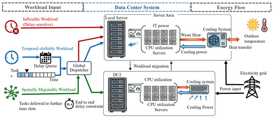
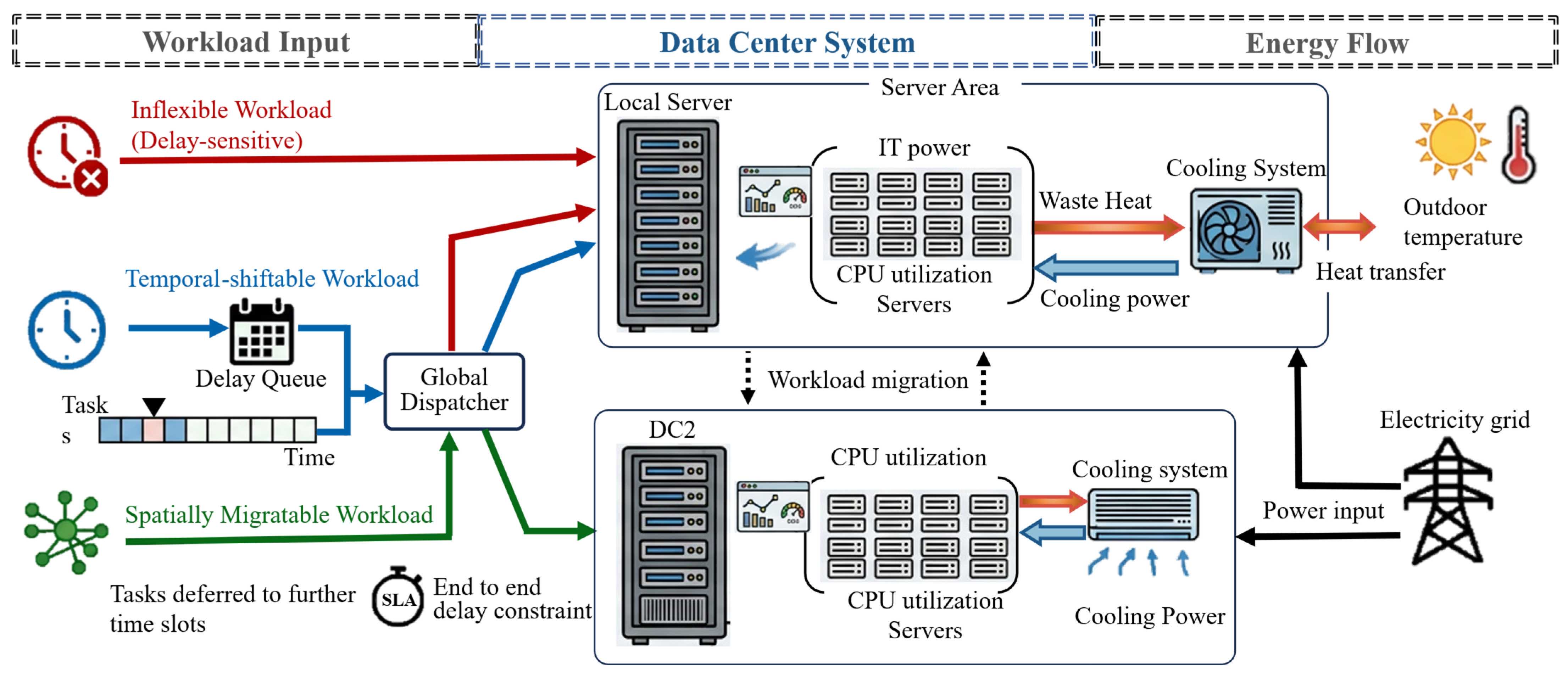
Figure 1 illustrates the architecture of the geo-distributed DC system. Each rectangular block in the figure represents a data center, within which the shaded regions denote server clusters and the associated cooling systems, capturing the IT power consumption and the cooling demand required to maintain indoor temperature constraints. Solid arrows between the data centers indicate possible workload migration paths for tasks that are spatially flexible, while dashed arrows represent temporal deferrable workloads that can be postponed to later time slots. This figure visually conveys how workload allocation, server utilization, cooling operation, and inter-DC network flows are interrelated, providing a clear reference for understanding how the temporal and spatial scheduling decisions described in this study influence operational cost and system performance.

2.2. Workload Model

In geo-distributed DC systems, workloads generated by users exhibit different levels of flexibility in both time and space. To capture the heterogeneous characteristics of computing tasks, the total workload in the system is categorized into three types: temporal-shiftable workloads, spatially migratable workloads, and inflexible workloads [23]. This classification allows the scheduler to exploit spatio-temporal flexibility to improve energy efficiency while satisfying service requirements.

Let ℕ denote the set of geo-distributed DCs, indexed by i, j ∈ ℕ. Let ℚ = {1, 2, ⋯, N_q} denote the set of scheduling time slots, indexed by t and τ. Unless otherwise stated, workload-related variables in this section are expressed as average workload rates during each scheduling time slot, measured in equivalent workload-unit rates.

Inflexible workloads must be processed at the DC where they are generated and cannot be delayed or migrated. Typical examples include real-time online services and interactive applications. These tasks must be processed locally, and thus can be expressed as:

$$L_{i,t}^{\mathrm{fix}}=W_{i,t}^{\mathrm{fix}}, \forall i\in \mathbb{N},t\in \mathbb{Q}$$

(1)

where $W_{i,t}^{\mathrm{fix}}$ and $L_{i,t}^{\mathrm{fix}}$ denote the inflexible workload arrival and locally processing at DC i during time slot t, respectively, measured in workload units per time slot.

Temporal-shiftable workloads are delay-tolerant tasks that can be deferred within a specified scheduling window. Typical examples include batch processing jobs, data analytics, and offline computing tasks. Temporal-shiftable workloads can be postponed within a maximum delay tolerance D, which is measured in the number of scheduling time slots. Let y_i,t,τ denote the amount of temporal-shiftable workload generated at DC i in time slot t and executed in time slot τ. The execution time τ must satisfy:

$$t\le \tau \le \min \left\{t+D,N_q\right\}$$

(2)

The temporal scheduling constraint can be expressed in (2), which ensures that all temporal-shiftable tasks are eventually processed within the allowable delay window.

$${\displaystyle \sum _{\tau =t}^{\min \left\{t+D,N_q\right\}}{y}_{i,t,\tau }}=W_{i,t}^{\mathrm{tem}}, \forall i\in \mathbb{N},t\in \mathbb{Q}$$

(3)

where $W_{i,t}^{\mathrm{tem}}$ denotes the temporal-shiftable workload arriving at DC i during time slot t. The amount of temporal-shiftable workload executed at DC i during time slot t is then given by:

$$L_{i,t}^{\mathrm{tem}}={\displaystyle \sum _{\tau =\max \left\{1,t-D\right\}}^t{y}_{i,t,\tau }}, \forall i\in \mathbb{N},t\in \mathbb{Q}$$

(4)

where $L_{i,t}^{\mathrm{tem}}$ represents the total temporal-shiftable workload executed at DC i during time slot t.

Spatially migratable workloads can be transferred among geographically distributed DCs to exploit differences in electricity prices, processing capability, or cooling efficiency.

Let x_i,j,t denote the amount of spatially migratable workload generated at source DC i and processed by destination DC j during time slot t. In this formulation, x_i,i,t represents the portion of spatially migratable workload that remains at the source DC and is processed locally. The spatial workload allocation constraint can therefore be expressed as:

$${\displaystyle \sum _{j\in \mathbb{N}}{x}_{i,j,t}}=W_{i,t}^{\mathrm{spa}}, \forall i\in \mathbb{N},t\in \mathbb{Q}$$

(5)

where $W_{i,t}^{\mathrm{spa}}$ denotes the spatially migratable workload arriving at DC i during time slot t. The total spatially migratable workload processed by DC j during time slot t is:

$$L_{j,t}^{\mathrm{spa}}={\displaystyle \sum _{i\in \mathbb{N}}{x}_{i,j,t}}, \forall j\in \mathbb{N},t\in \mathbb{Q}$$

(6)

Thus, the total workload processed at DC i during time slot t is:

$$L_{i,t}=L_{i,t}^{\mathrm{fix}}+L_{i,t}^{\mathrm{tem}}+L_{i,t}^{\mathrm{spa}}, \forall i\in \mathbb{N},t\in \mathbb{Q}$$

(7)

Substituting (1), (3), and (5) into (6), the processed workload can also be written as:

$$L_{i,t}=W_{i,t}^{\mathrm{fix}}+{\displaystyle {\displaystyle \sum _{\tau =\max \left\{1,t-D\right\}}^t}{y}_{i,t,\tau }}+{\displaystyle {\displaystyle \sum _{j\in \mathbb{N}}}{x}_{j,i,t}}, \forall i\in \mathbb{N},t\in \mathbb{Q}$$

(8)

This formulation avoids double-counting and ensures workload conservation across both temporal shifting and spatial migration. In particular, outgoing spatially migratable workloads from DC i are not included in L_i,t unless they are assigned to be processed at i through x_i,j,t.

2.3. Energy Consumption Model of Data Center

Most of the energy consumption in DCs comes from IT equipment operation and the cooling system. The IT equipment’s power consumption mainly depends on the amount of workloads. To ensure the equipment can operate at a suitable temperature, the cooling system power should be adjusted promptly. Cooling system provides thermal cooling power to eliminate the heat generated by IT equipment as well as the heat transferred from outdoors, to maintain the internal ambient temperature of DCs. Therefore, the energy consumption of DC in this paper is divided into three parts: IT equipment, cooling system, and other equipment.

$$P_{i,t}^{\mathrm{DC}}=P_{i,t}^{\mathrm{IT}}+P_{i,t}^{\mathrm{cool}}+P_{i,t}^{\mathrm{oth}} , \forall i\in \mathbb{N},t\in \mathbb{Q}$$

(9)

where $P_{i,t}^{\mathrm{IT}}$, $P_{i,t}^{\mathrm{cool}}$ and $P_{i,t}^{\mathrm{oth}}$ denote the IT power consumption, cooling power consumption, and auxiliary power consumption of DC i during time slot t, respectively, measured in MW. $P_{i,t}^{\mathrm{DC}}$ is the power purchased from the electricity grid.

The power consumption of a server is typically related to its CPU utilization level. Empirical studies show that even when a server is idle, it still consumes a significant portion of its peak power. Therefore, the server power consumption can be modeled as a linear function of CPU utilization [19].

Let N_i denote the total number of servers installed in DC i, and let n_i,t denote the number of active servers in DC i during time slot t. Both N_i and n_i,t are count variables. The server provisioning constraint is:

$$0\le n_{i,t}\le N_i$$

(10)

Let u_i,t denote the average CPU utilization of servers in DC i at time slot t, which is dimensionless. And let μ denote the service capacity of one active server. Then

$$u_{i,t}={\displaystyle \frac{L_{i,t}}{n_{i,t}\mu }}$$

(11)

Equivalently, the server capacity constraint can be written in linear form as:

$$0\le u_{i,t}\le u^{\max }$$

(12)

$$L_{i,t}\le u^{\max }\mu n_{i,t}$$

(13)

The IT power consumption is modeled as a linear function of server utilization:

$$P_{i,t}^{\mathrm{IT}}=n_{i,t}\left[P^{\mathrm{idle}}+\left(P^{\mathrm{peak}}-P^{\mathrm{idle}}\right)u_{i,t}\right]$$

(14)

where P^idle and P^peak denote the idle power and peak power of a server, respectively.

Actually, the cooling load power consumption consists mainly of two parts. One is the internal load caused by the heat of IT equipment from workload processing [21]. The other is the external disturbance load caused by heat transfer under the influence of external periodical weather [26]. The relationships among the computing power, cooling power, and indoor/outdoor temperatures can be derived via the ETP model.

$$C_i{\displaystyle \frac{\mathrm{d}{T}_{i,t}^{\mathrm{in}}}{\mathrm{d}t}}={\displaystyle \frac{T_{i,t}^{\mathrm{out}}-T_{i,t}^{\mathrm{in}}}{R_i}}+Q_{i,t}^{\mathrm{DC}}$$

(15)

$$Q_{i,t}^{\mathrm{DC}}=(k^{\mathrm{IT}}{P}_{i,t}^{\mathrm{IT}}-k^{\mathrm{cop}}{P}_{i,t}^{\mathrm{cool}})$$

(16)

where $T_{i,t}^{\mathrm{in}}$ and $T_{i,t}^{\mathrm{out}}$ are the indoor and outdoor air temperatures, measured in °C; $Q_{i,t}^{\mathrm{DC}}$ is the total thermal power of DC, measured in MW; $k^{\mathrm{IT}}$ is the heat factor of IT equipment and is dimensionless; and k^cop is the energy efficiency ratio of the cooling system and is dimensionless; C_i is the heat capacity of the indoor air, measured in MWh/°C; R_i is the thermal resistance between the indoor air and the external environment, measured in °C/MWh. The analytical recursive form of (15) can be expressed as:

$$T_{i,t}^{\mathrm{in}}=T_{i,t-1}^{\mathrm{in}}{e}^{-{\displaystyle \frac{1}{R_i{C}_i}}}+\left(1-e^{-{\displaystyle \frac{1}{R_i{C}_i}}}\right)\left(T_{i,t}^{\mathrm{out}}+R_i{Q}_{i,t}^{\mathrm{DC}}\right)$$

(17)

Based on the combination of (15)–(17), the cooling system power consumption calculation by means of the ETP model is deduced as follows:

$$\left\{\begin{array}{l}{Q}_{i,t}^{\mathrm{DC}}={\displaystyle \frac{\left(T_{i,t}^{\mathrm{in}}-e^{-\frac{1}{R_i{C}_i}}{T}_{i,t-1}^{\mathrm{in}}\right)}{R}}-\left(1-e^{-{\displaystyle \frac{1}{R_i{C}_i}}}\right){\displaystyle \frac{T_{i,t}^{\mathrm{out}}}{R_i}}\\ P_{i,t}^{\mathrm{cool}}=\left(k^{\mathrm{IT}}{P}_{i,t}^{\mathrm{IT}}-Q_{i,t}^{\mathrm{DC}}\right)/k^{\mathrm{cop}}\end{array}\right.$$

(18)

It can be seen from (18) that the cooling system provides thermal cooling power to eliminate the heat generated by IT and other equipment, and the heat transferred from the outdoors.

The indoor temperature must be maintained within an acceptable range:

$$T_{\min }^{\mathrm{in}}\le T_{i,t}^{\mathrm{in}}\le T_{\max }^{\mathrm{in}}$$

(19)

To avoid excessive temperature fluctuation, the temperature variation between adjacent time slots is limited by:

$$\left|T_{i,t}^{\mathrm{in}}-T_{i,t-1}^{\mathrm{in}}\right|\le \Delta T_{\max }^{\mathrm{in}}$$

(20)

where $T_{\min }^{\mathrm{in}}$ and $T_{\max }^{\mathrm{in}}$ denote the minimum and maximum indoor temperature in the DC, measured in °C. ${\Delta T}_{\max }^{\mathrm{in}}$ is the maximum variation in indoor temperature.

2.4. Inter-Data-Center Network Model

In geographically distributed DC systems, workload migration among DCs inevitably incurs communication delays and consumes inter-DC network capacity. The inter-DC network is modeled at the workload-scheduling level, with a fixed logical path assumed for each source–destination DC pair during each scheduling interval. The bandwidth constraint limits the migrated workload on each link and thereby represents network congestion at an aggregate level. The end-to-end delay comprises propagation, transmission, and destination-side processing delays, which jointly affect service quality. Dynamic routing, packet-level queuing, and short-term congestion fluctuations are not explicitly considered because this study focuses on hourly workload scheduling rather than the real-time network control.

Spatial workload migration incurs communication delay and is constrained by the available bandwidth of inter-DC links. For a workload migrated from source DC i to destination DC j, the end-to-end delay consists of propagation delay, transmission delay, and processing delay. Let d_i,j denote the geographical distance between DC i and DC j. And let v denote the signal propagation speed in optical fiber, measured in km/s. The propagation delay ${\delta }_{i,j}^{\mathrm{prop}}$ is:

$${\delta }_{i,j}^{\mathrm{prop}}={\displaystyle \frac{d_{ij}}{v}} , \forall i,j\in \mathbb{N}$$

(21)

Let S denote the average data size associated with one unit of migrated workload, and let BW_ij denote the available bandwidth of the communication link between DC i and DC j, measured in Gbps. The transmission delay of a unit migrated workload ${\delta }_{i,j}^{\mathrm{trans}}$, and the bandwidth capacity constraint are:

$${\delta }_{i,j}^{\mathrm{trans}}={\displaystyle \frac{S}{B{W}_{ij}}}, \forall i,j\in \mathbb{N}, i\ne j$$

(22)

$$x_{i,j,t}S\le B{W}_{ij}, \forall i,j\in \mathbb{N}, i\ne j,t\in \mathbb{Q}$$

(23)

Processing delay corresponds to the time required for a task to be processed at the destination DC after arrival. In this work, the task processing behavior is modeled using an M/M/1 queuing system, which is widely adopted for modeling service systems with stochastic arrivals and exponential service times [23,27].

Let m_j,t denote the effective service rate of DC j during time slot t, then

$$m_{j,t}=\mu n_{j,t}$$

(24)

Let λ_j,t denote the total workload arrival rate assigned to DC j during time slot t. The expected processing delay ${\delta }_{i,j}^{\mathrm{proc}}$ is then expressed as:

$${\delta }_{j,t}^{\mathrm{proc}}={\displaystyle \frac{1}{m_{j,t}-{\lambda }_{j,t}}}={\displaystyle \frac{1}{\mu n_{j,t}-{\lambda }_{j,t}}}, \forall j\in \mathbb{N}, t\in \mathbb{Q}$$

(25)

Therefore, the end-to-end delay of a workload migrated from DC i to DC j during time slot t is:

$${\delta }_{i,j,t}^{\mathrm{delay}}={\delta }_{i,j}^{\mathrm{prop}}+{\delta }_{i,j}^{\mathrm{trans}}+{\delta }_{j,t}^{\mathrm{proc}}$$

(26)

To guarantee quality of service, the delay must satisfy:

$${\delta }_{i,j,t}^{\mathrm{delay}}\le {\delta }^{\max }, \forall i,j\in \mathbb{N}, i\ne j,t\in \mathbb{Q}$$

(27)

where δ^max denotes the maximum tolerable end-to-end delay, measured in seconds.

3. Two-Stage Stochastic Energy-Efficient Optimal Scheduling Model of Geo-Distributed Data Centers

Based on the geo-distributed DC system model described in Section 2, this section develops a two-stage stochastic optimization model for workload scheduling under uncertainty. Different from a pure energy-minimization formulation, the primary objective in this work is to minimize the total electricity cost of the geo-distributed DC system over the scheduling horizon. This formulation is more consistent with the practical operation of interconnected DCs, where regional electricity prices, workload flexibility, and cooling conditions jointly determine the economic performance of the system. Within this framework, temporal workload shifting and spatial workload migration are coordinated to reshape the workload distribution across both time and location, while server operation, cooling demand, and network constraints are explicitly taken into account. The resulting model, therefore, seeks a cost-optimal scheduling plan that remains feasible and adaptive under uncertain workload realizations.

3.1. Workload Uncertainty and Scenario Construction

Let K = {fix, tem, spa} denote the set of workload types, corresponding to inflexible, temporal-shiftable, and spatially migratable workloads, respectively. For each DC i ∈ ℕ, time slot t ∈ ℚ, and workload type k ∈ K, the forecasted workload is denoted by $W_{i,t}^k$. The scenario-dependent workload realization is denoted by $W_{i,t}^{k,\omega }$, where ω represents a workload scenario.

The uncertain workload is modeled by a bounded multiplicative forecast error:

$$W_{i,t}^{k,\omega }=W_{i,t}^k\left(1+{\epsilon }_{i,t}^{k,\omega }\right), \forall i\in \mathbb{N}, t\in \mathbb{Q},k\in \mathbf{K}$$

(28)

where ${\epsilon }_{i,t}^{k,\omega }$ denotes the normalized forecast error of workload type k at DC i during time slot t under scenario ω, which is dimensionless. In this work, the forecast error is generated from a bounded uniform distribution:

$${\epsilon }_{i,t}^{k,\omega }\sim U\left[-\rho ,\rho \right]$$

(29)

where ρ denotes the workload fluctuation level and is dimensionless. For each scenario ω, all workload realizations are collected into the uncertainty vector:

$${\mathbf{\xi }}^{\omega }={\left[W_{i,t}^{k,\omega }\right]}_{i\in \mathbb{N}, t\in \mathbb{Q},k\in \mathbf{K}}$$

(30)

In the considered three-DC system with 24 hourly time slots and three workload categories, each scenario contains 216 uncertain workload components. Latin Hypercube Sampling (LHS) is adopted to generate the initial workload scenario set [28]. Compared with simple random sampling, LHS improves the coverage of the uncertainty space by stratifying the distribution of each uncertain variable. In this study, N_s initial scenarios are generated. For each uncertain workload component, the cumulative probability interval is divided into N_s equal-probability intervals, and one sample is randomly drawn from each interval. For the uniform distribution in (29), the sampled forecast error can be calculated as:

$${\epsilon }_{i,t}^{k,\omega }=-\rho +2\rho r_{i,t}^{k,\omega }$$

(31)

where $r_{i,t}^{k,\omega }$ ∈ [0, 1] is the sampled cumulative probability value for scenario ω_s, which is dimensionless. The corresponding workload realization is then obtained using (28). The initial scenario set is denoted by Ω⁰, and all initial scenarios are assigned equal probabilities.

3.2. Fast Forward Scenario Reduction for Two-Stage Stochastic Scheduling

For the proposed two-stage stochastic scheduling (TSS) model, directly incorporating all workload scenarios generated by Latin hypercube sampling would lead to a large-scale deterministic equivalent formulation. Therefore, the Fast Forward scenario reduction method is used to reduce the computational burden while preserving the main characteristics of the original scenario set [29]. In this work, N_r representative scenarios are retained, and the reduced scenario set is denoted by Ω.

The dissimilarity between two workload scenarios ω and ω′ is measured by the normalized Euclidean distance:

$$d\left(\omega ,{\omega }^{\prime }\right)=\sqrt{{\displaystyle \sum _{k\in \mathbf{K}}{\displaystyle \sum _{i\in \mathbb{N}}{\displaystyle \sum _{t\in \mathbb{Q}}{\left(\frac{W_{i,t}^{k,\omega }-W_{i,t}^{k,{\omega }^{\prime }}}{W_{i,t}^k}\right)}^2}}}}$$

(32)

where d(ω, ω′) is a normalized Euclidean distance between two scenarios and is dimensionless after normalization. The normalization by $W_{i,t}^k$ avoids the distance metric being dominated by workload components with large numerical magnitudes.

The Fast Forward algorithm starts from an empty reduced set and iteratively adds the scenario that yields the largest reduction in the weighted distance between the original and reduced scenario sets. After the representative scenarios are selected, the probability of each removed scenario is reassigned to its nearest retained scenario. The updated probability of a retained scenario $\tilde{\omega }$∈ Ω is given by:

$$\left\{\begin{array}{l}{p}_{{\omega }^{\prime }}=p_{{\omega }^{\prime }}^0+{\displaystyle \sum _{\omega \in {\mathsf{\Omega }}^0}{p}_{\omega }^0}\\ {\omega }^{\prime }=\arg {\displaystyle \underset{{\omega }^{\prime }\in \mathsf{\Omega }}{\min }}d\left(\omega ,{\omega }^{\prime }\right)\end{array}\right.$$

(33)

where $P_{\omega }^0$ is the initial probability of scenario ω. The updated probabilities satisfy:

$${\displaystyle \sum _{\omega \in \mathsf{\Omega }}{p}_{\omega }}=1$$

(34)

Through LHS and Fast Forward scenario reduction, the continuous workload uncertainty is approximated by a finite set of representative scenarios. This setting provides a practical balance between uncertainty representation and computational tractability.

3.3. Two-Stage Decision Structure and Scenario-Wise Constraints

The proposed stochastic scheduling model follows a two-stage decision structure. The first-stage decision is made before the realization of workload uncertainty, while the second-stage recourse decisions are made after a specific workload scenario is observed.

The first-stage decision variable is the active server provisioning plan:

$$\mathit{n}=\left\{n_{i,t}\left|i\in \mathbb{N}, t\in \mathbb{Q}\right.\right\}$$

(35)

Since this decision is determined before the workload scenario is known, it is non-anticipative and shared by all scenarios. For each scenario ω ∈ Ω, the second-stage recourse variables are collected as:

$${\mathit{z}}^{\omega }=\left\{{\mathit{y}}^{\omega },{\mathit{x}}^{\omega },{\mathit{L}}^{\omega },{\mathit{u}}^{\omega },{\mathit{P}}^{\omega },{\mathit{q}}^{\omega }\right\}$$

(36)

where y^ω denotes temporal workload shifting decisions, x^ω denotes spatial workload migration decisions, L^ω denotes processed workloads, u^ω denotes server utilizations, P^ω denotes IT, cooling, and grid-side power variables, and q^ω denotes delay-related variables.

The first-stage feasible set is defined as:

$$\mathit{\chi }=\left\{\mathit{n}\left|0\le n_{i,t}\le N_i, \forall i\in \mathbb{N}, t\in \mathbb{Q}\right.\right\}$$

(37)

where N_i denotes the total number of servers installed in DC i. Given the first-stage decision n and the workload realization ξ^ω, the scenario-wise second-stage feasible set is represented by:

$${\mathit{z}}^{\omega }\in \mathit{\gamma }\left(\mathit{n},{\mathit{\xi }}^{\omega }\right), \forall \omega \in \mathsf{\Omega }$$

(38)

The feasible set γ(n, ξ^ω) is obtained by imposing the deterministic constraints developed in Section 2 under scenario ω, with deterministic workload parameters replaced by their scenario-dependent realizations $W_{i,t}^{k,\omega }$. Specifically, it includes workload conservation constraints, delay-window constraints for temporal workload shifting, spatial workload allocation constraints, server capacity and utilization constraints, IT and cooling power constraints, indoor temperature dynamic constraints, bandwidth constraints, end-to-end delay constraints, and non-negativity constraints.

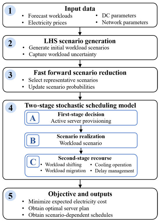
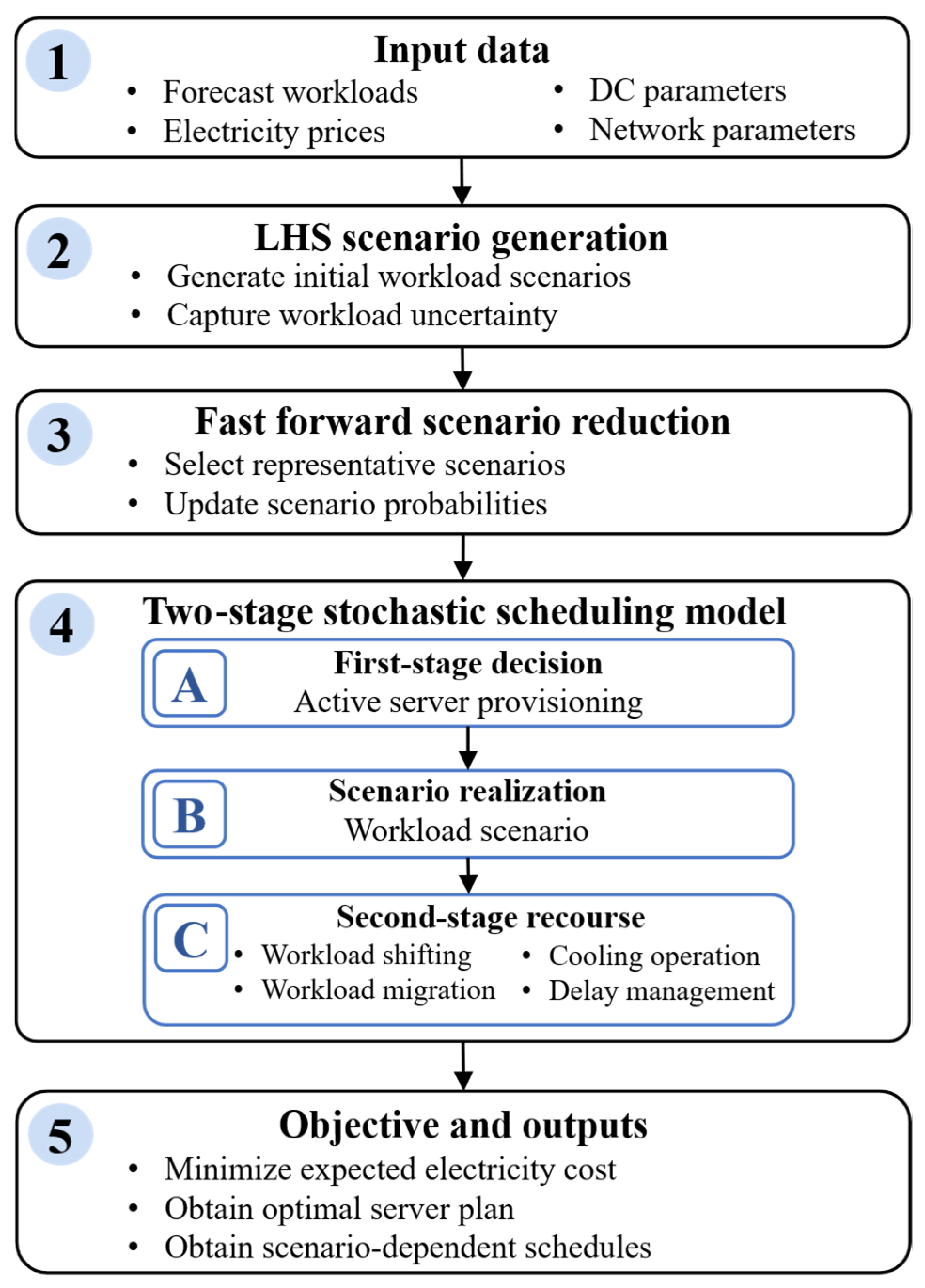
Therefore, all operational constraints must hold for every retained scenario, while the same first-stage server provisioning plan n is shared across all scenarios. Non-anticipativity is thus enforced by using the common scenario-independent variable n_i,t. The overall workflow of the proposed stochastic scheduling framework is illustrated in Figure 2, where the scenario construction process, the first-stage non-anticipative decision, and the second-stage scenario-dependent recourse decisions are explicitly distinguished.

3.4. Objective Function

Given the first-stage decision n and workload realization ξ^ω, the second-stage recourse function is defined as the minimum operating cost under scenario ω:

$$Q\left(\mathit{n},{\mathit{\xi }}^{\omega }\right)={\displaystyle \underset{{\mathit{z}}^{\omega }\in \mathit{\gamma }\left(\mathit{n},{\mathit{\xi }}^{\omega }\right)}{\min }}{\displaystyle \sum _{i\in \mathbb{N}}{\displaystyle \sum _{t\in \mathbb{Q}}{\pi }_{i,t}{P}_{i,t}^{\mathrm{DC}}}\Delta t}$$

(39)

where π_i,t is the electricity price of DC i at time slot t, and Δt is the duration of one scheduling time slot, measured in hours. Based on the recourse function and the scenario-wise feasible set, the two-stage stochastic scheduling problem can be formulated as:

$$\begin{array}{l}{J}^{\ast }=\min \sum p_{\omega }Q\left(\mathit{n},{\mathit{\xi }}^{\omega }\right)\\ \mathrm{s}.\mathrm{t}. \mathit{n}\in \mathit{\chi },\omega \in \mathsf{\Omega }\end{array}$$

(40)

where J* denotes the optimal expected operating cost. n is the first-stage non-anticipative decision variable shared by all scenarios, while z^ω represents the second-stage recourse variables associated with scenario ω. The deterministic equivalent formulation explicitly enforces all workload scheduling, server operation, cooling, thermal, bandwidth, and delay constraints for every retained workload scenario.

4. Simulation Experiments and Result Analysis

To validate the effectiveness of the proposed two-stage stochastic scheduling framework, this section presents a series of simulation experiments and comparative analyses. The experiments are designed to evaluate the performance of the proposed method in managing geo-distributed DC operations under uncertain workload conditions while exploiting both temporal and spatial workload flexibility. All optimization problems are solved using YALMIP [30] (version 20230622) with the Gurobi solver [31] (version 11.0.1) on a workstation equipped with an Intel Core i7 processor and 32 GB RAM.

4.1. Basic Data and Parameter Settings

Numerical experiments are conducted on a geo-distributed DC system composed of three interconnected facilities. The scheduling horizon is set to 24 h, discretized into hourly time slots, which allows the framework to capture both temporal workload shifting and inter-DC migration within a daily operational cycle. To improve the realism of the case study, historical workload traces collected from an operational data center in China were used to construct the baseline workload profiles. The dataset covers the period from January to July in 2025 with a sampling interval of 1 h. The collected records include workload demand, IT power consumption, cooling power consumption, indoor/outdoor temperature, and server operation status. During preprocessing, records with missing timestamps or physically invalid values were removed, isolated missing values were interpolated, and all variables were aligned to hourly intervals. A representative 24 h profile was then obtained from the processed records and used as the baseline input for the simulations. Workloads are classified according to their permissible temporal and spatial scheduling actions. Inflexible workloads must be processed locally without delay, temporal-shiftable workloads can be deferred within the specified time window, and spatially migratable workloads can be transferred among DCs subject to bandwidth and latency constraints.

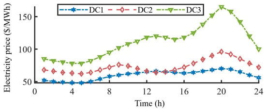
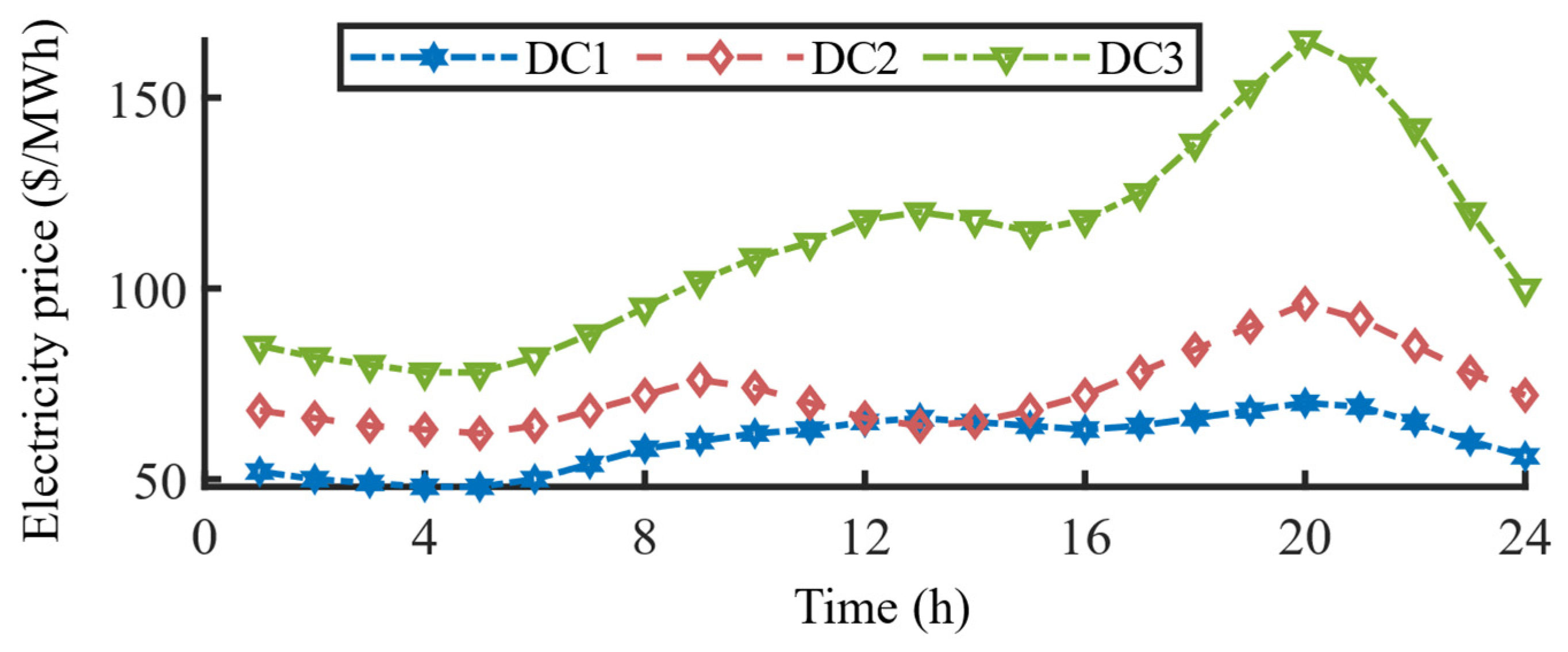
The three data centers are heterogeneous in terms of electricity prices, processing capabilities, and thermal conditions. The hourly electricity price profiles are shown in Figure 3. DC1 has a moderate electricity price and average processing capacity, DC2 is located in a region with lower electricity prices but higher cooling requirements due to warmer ambient conditions, and DC3 has a higher electricity price but more efficient cooling infrastructure. The parameters listed in

Table 2. The Parameters of the GEO-Distributed DCs System.

Parameter Group	Parameter	Value
IT Equipment	Pidle/Ppeak	0.5/0.9 × 10−3 MW
	μ	1 × 103 request/s
	n1, n2, n3	2200, 2200, 2200
	δmax	0.100 s
	BW	100 Gbps
	v	2 × 105 km/s
	umax	0.7
Cooling System	kIT	0.3
	${\Delta T}_{\max }^{\mathrm{in}}$	3 °C
	Ci	0.166 MWh/°C
	Ri	0.61 × 103 °C/MWh
	$T_{\min }^{\mathrm{in}}$/$T_{\max }^{\mathrm{in}}$	15/25 °C
	$k_i^{\mathrm{cop}}$	1.027
Uncertainty	Ns, Nr	2000, 100

, including server counts, CPU utilization limits, power ratings, thermal capacities, and network bandwidths, are based on real measurements and operational specifications from the source data center and are representative of typical medium-scale geo-distributed DC systems. This setup ensures that the simulation results reflect realistic operational conditions and accurately evaluate the effectiveness of the proposed scheduling framework.

4.2. Ablation Study on Workload Flexibility

To investigate the individual contributions of temporal workload shifting and spatial workload migration, an ablation study is conducted in four cases:

• C1: Workloads are processed locally without spatial migration or temporal shifting.
• C2: Workloads are processed locally with temporal shifting, but no spatial migration is allowed.
• C3: Workloads can be migrated among DCs, but no temporal shifting is allowed.
• C4: Both workload spatial migration and temporal shifting are allowed under deterministic demand.

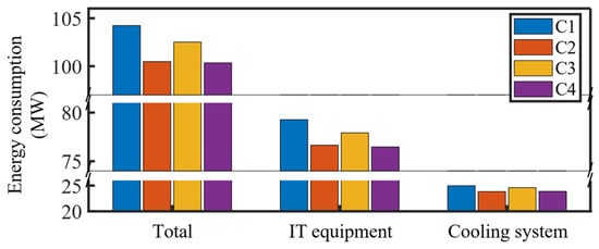
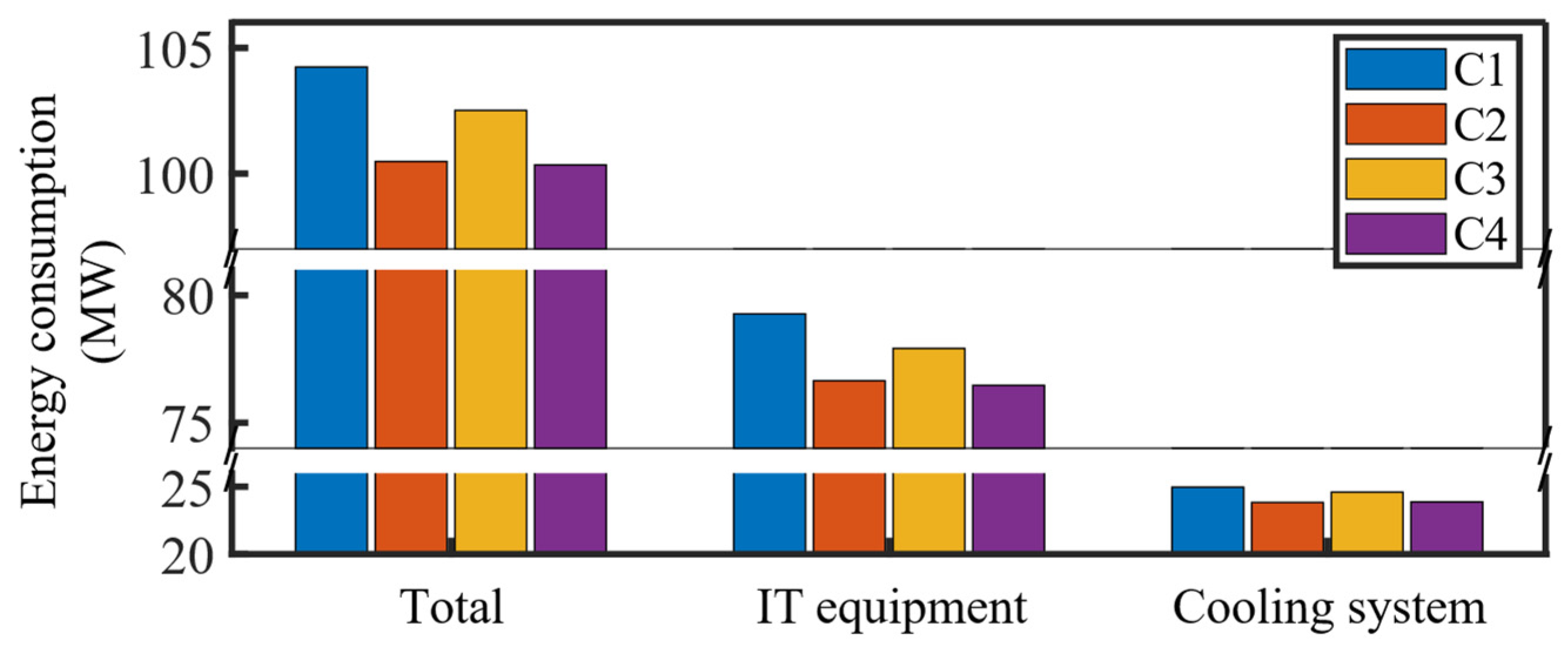
The results of the ablation study are summarized in

Table 3. Performance comparison of different flexibility mechanisms.

Case	Time Shifting	Spatial Migration	Total Energy (MWh)	Total Cost (106 $)	Average Active Servers	Average Utilization (%)
C1	-	-	104.24	8.146	1443	65.73
C2	√	-	100.48	7.775	1370	69.15
C3	-	√	105.51	7.838	1406	67.37
C4	√	√	100.34	7.594	1365	69.41

, where different combinations of temporal workload shifting and spatial workload migration are evaluated. Compared with the baseline case without flexibility (C1), enabling temporal shifting only (C2) reduces the total energy consumption from 104.24 MWh to 100.48 MWh, corresponding to an energy reduction of approximately 3.6%. This improvement is mainly attributed to the ability to defer delay-tolerant workloads across time periods, which reduces the number of active servers from 1443 to 1370 and increases the average server utilization from 65.73% to 69.15%. In contrast, enabling spatial migration only (C3) reduces the total operating cost but slightly increases total energy consumption from 104.24 MWh to 105.51 MWh. This result indicates that spatial migration is primarily driven by electricity-price differences and network feasibility rather than energy minimization alone. Some workloads are therefore migrated to lower-price DCs even when the destination DCs require more active servers or face less favorable cooling conditions. In such cases, workload concentration may increase local server activation and cooling demand, leading to higher total energy use despite lower electricity cost. This also shows that spatial migration is more beneficial when the destination DC has not only a lower electricity price but also sufficient server capacity, available bandwidth, acceptable delay, and favorable cooling efficiency.

The best performance (in bold) is achieved when both temporal shifting and spatial migration are jointly enabled (C4). In this configuration, total energy consumption decreases to 100.34 MWh, achieving an overall reduction of approximately 3.7% compared with C1, while the number of active servers further decreases to 1365 and the average utilization increases to 69.41%, the highest among all cases. This result suggests that temporal shifting and spatial migration are complementary rather than simply additive. Temporal shifting first alleviates peak-time workload congestion and reduces the cooling burden during high-load or thermally unfavorable periods, while spatial migration further reallocates the remaining flexible workloads across DCs according to electricity price, capacity, cooling, and network constraints. Therefore, the joint strategy provides a better balance between energy saving, cost reduction, and resource utilization.

To further illustrate the energy-saving mechanisms of different workload flexibility strategies, Figure 4 compares the relative reductions in IT energy, cooling energy, and total energy with respect to the no-flexibility case. Temporal shifting yields a more pronounced reduction in IT energy because it lowers peak server activation and improves temporal load balancing. The reduction in cooling energy follows the same trend, indicating a direct interaction between server utilization and cooling demand: lower IT power reduces internal heat generation and consequently decreases the required cooling power. Spatial migration alone provides limited energy savings because its effectiveness depends on the thermal conditions of the destination DCs. When high workload periods coincide with high outdoor temperature or low cooling efficiency, temporal shifting tends to be more effective than migration for energy reduction, since it can defer delay-tolerant workloads to cooler or less congested periods.

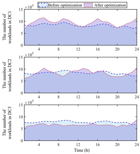
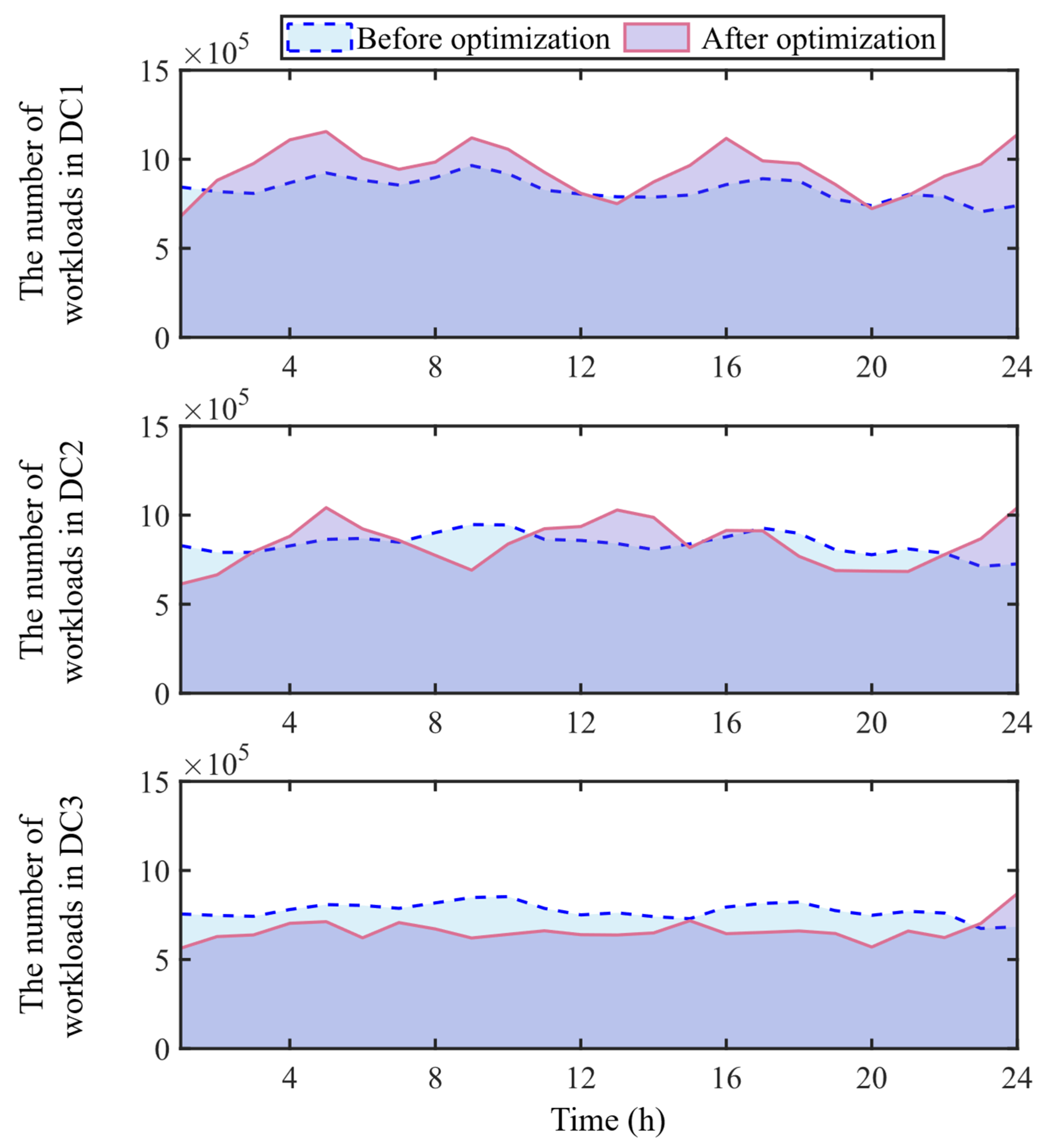
Figure 5 illustrates the hourly workload redistribution of the three geo-distributed DCs before and after applying the proposed scheduling strategy. Compared with the original workload profiles, noticeable changes can be observed after optimization. In particular, the workload processed by DC1 increases during multiple time periods, with an average increase of approximately 8–10%, indicating that additional flexible tasks are migrated to DC1 due to its more favorable operating conditions. The workload of DC2 shows moderate temporal adjustments, with an average increase of about 3–5%, suggesting that DC2 participates in balancing system workloads during certain hours. In contrast, the workload of DC3 decreases significantly, with an average reduction of approximately 12–15%, as part of its tasks are transferred to other DCs with lower operating costs. Overall, these results demonstrate that the proposed scheduling framework effectively exploits spatial workload migration and temporal workload shifting to achieve a more balanced workload distribution and improved utilization of geo-distributed DC resources.

4.3. Impact of Workload Uncertainty on Scheduling Performance

To further examine the role of stochastic uncertainty modeling, this subsection investigates how different levels of workload uncertainty affect the scheduling decisions and system performance of the proposed framework. Unlike a purely deterministic analysis based on a single forecast, the proposed two-stage stochastic model makes first-stage decisions that are shared across all reduced scenarios, while second-stage recourse decisions are adaptively adjusted after the uncertainty is realized. Such a structure enables the scheduler to explicitly account for possible workload fluctuations and to maintain feasible and reliable operation under multiple demand realizations.

In this experiment, the workload fluctuation range is used as the main uncertainty parameter. Four uncertainty levels are considered, namely ±5%, ±10%, ±15%, and ±20%. The purpose of this experiment is to reveal how the proposed stochastic framework responds to increasingly uncertain workloads in terms of energy consumption, operating cost, server provisioning, and resource utilization.

As shown in

Table 4. Performance comparison of the proposed stochastic scheduling framework under different workload uncertainty levels.

Workload Fluctuation Range	Total Cost (106 $)	Total Energy (MWh)	Average Active Servers	Average Utilization (%)
±5%	7.57	100.12	1360	69.70
±10%	7.59	100.34	1365	69.41
±15%	7.61	100.57	1371	69.13
±20%	7.64	100.80	1376	68.86

, the proposed framework exhibits a clear yet moderate response to increasing workload uncertainty. When the fluctuation range increases from ±5% to ±20%, the total energy consumption rises only slightly from 100.12 MWh to 100.80 MWh, while the total operating cost increases from 7.57 × 10⁶ $ to 7.64 × 10⁶ $. These results indicate that larger uncertainty indeed requires additional resources to hedge against adverse scenarios, but the overall increase in system cost and energy use remains limited. This suggests that the proposed stochastic scheduling model can absorb workload variability without causing significant deterioration in overall operating efficiency. A more informative change can be observed in the server-side operational indicators. As workload uncertainty becomes stronger, the average number of active servers increases from 1360 to 1376, whereas the average server utilization decreases slightly from 69.70% to 68.86%. This trend reflects the essential mechanism of the two-stage stochastic model: to remain feasible under multiple potential workload realizations, the scheduler proactively maintains a slightly larger online server pool as a capacity buffer. As a result, the system sacrifices a small amount of average utilization in exchange for improved adaptability and robustness against high-demand scenarios. These results show that uncertainty modeling does not merely alter the objective value numerically; more importantly, it changes the operational strategy of the system. Under higher uncertainty, the scheduler becomes more conservative in capacity provisioning and avoids overly tight resource consolidation. Therefore, the value of stochastic optimization lies not only in optimizing expected performance, but also in producing schedules that remain stable and implementable when the actual workload deviates from its nominal forecast.

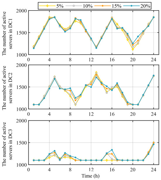
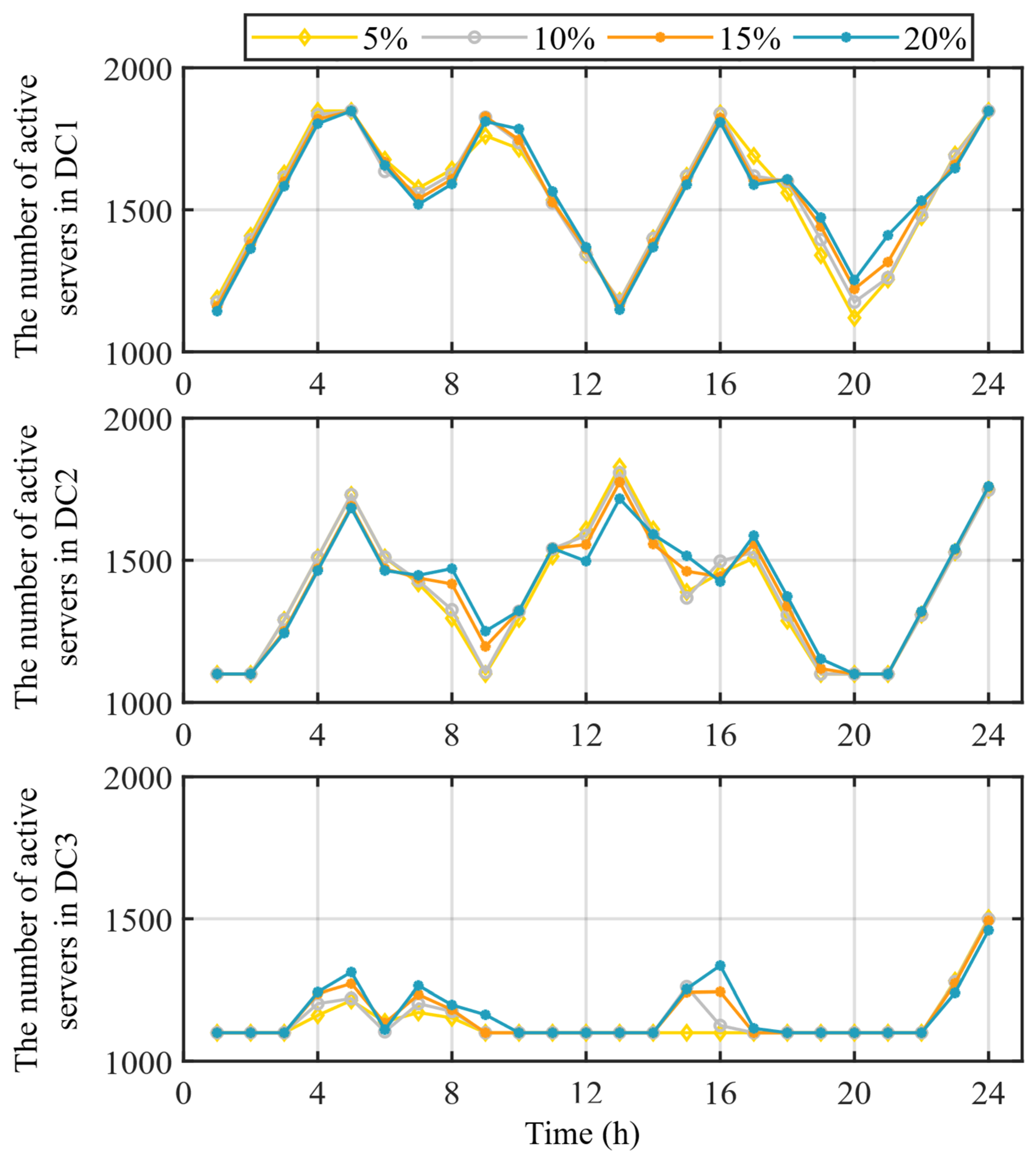
Figure 6 compares the hourly active server schedules of the three DCs under different workload uncertainty levels. It can be seen that the server activation profiles under different uncertainty levels generally follow similar daily patterns, indicating that the proposed stochastic framework preserves the overall temporal scheduling structure. Meanwhile, noticeable differences appear in several peak and transition periods, where the active server numbers are adjusted to accommodate different workload realizations. This suggests that workload uncertainty mainly affects the fine-grained capacity reservation of individual DCs rather than the overall scheduling trend. In addition, the adjustments occur at different hours and with different magnitudes in DC1, DC2, and DC3, showing that workload uncertainty is handled through differentiated local responses across the three DCs.

Overall, the above results confirm that explicit stochastic treatment of workload uncertainty is essential for reliable geo-distributed DC scheduling. As uncertainty increases, the proposed framework responds by moderately expanding server provisioning and accepting a slight reduction in average utilization, while keeping the growth of total energy consumption and operating cost at a relatively low level. This demonstrates that the proposed model achieves a desirable balance between energy efficiency and operational robustness, which is particularly important for practical DC systems facing uncertain and time-varying demand.

4.4. Comparison with Deterministic and Robust Optimization

To further evaluate the value of the proposed two-stage stochastic scheduling framework, two benchmark methods are considered: deterministic optimization (DO) and robust optimization (RO) [32,33]. In DO, the uncertain workloads are replaced by their expected values, and the scheduling problem is solved under the nominal scenario. In RO, the scheduling decision is optimized against the worst-case operating condition constructed from the training scenario set. Specifically, for a given first-stage decision, the operating cost is evaluated under all scenarios in the training set, and the scenario producing the highest cost is identified as the worst-case scenario. The proposed method, denoted as TSS, minimizes the expected operating cost over the reduced representative scenario set and allows recourse decisions to adapt to each realized scenario. For a fair comparison, all methods are trained using the same historical data and evaluated on the same 2000 out-of-sample scenarios. The testing scenarios include Gaussian perturbations, moment perturbations, and Weibull long-tail disturbances, representing normal forecast errors, distributional shifts, and extreme operating conditions, respectively.

The cost-risk performance is evaluated using the mean cost, median cost, cost standard deviation (Std.), 99th percentile cost (Q99), and conditional value-at-risk at the 95% confidence level (CVaR_0.95). The 99th percentile cost measures the upper-tail operating cost, while CVaR0.95 is computed as the average cost of the worst 5% out-of-sample scenarios.

Table 5. Out-of-sample cost-risk comparison.

Method	Mean (106 $)	Median (106 $)	Std. (106 $)	Q99 (106 $)	CVaR0.95 (106 $)	Policy Optimization Time (s)	Mean Recourse Evaluation Time (s/Scenario)
DO	7.90	7.69	0.45	9.02	8.96	0.14	0.10
RO	8.54	8.51	0.08	8.73	8.72	15.90	0.06
TSS	7.84	7.63	0.39	8.88	8.82	33.50	0.05

reports the out-of-sample cost-risk performance of the three methods. DO has the largest cost fluctuation and the highest upper-tail cost among the three methods. This indicates that optimizing only the nominal scenario is insufficient when the realized workloads deviate from their expected values. Although DO achieves a lower average cost than RO, it exposes the system to higher tail risk. RO achieves the lowest cost standard deviation, Q99 cost, and CVaR_0.95 cost. This is because RO explicitly protects the scheduling decision against the worst-case operating condition. However, such risk protection is obtained at the expense of a much higher mean and median operating cost. Specifically, the mean cost of RO reaches $8.54 × 10⁶, which is higher than those of DO and TSS. This confirms the conservative nature of the robust benchmark. Compared with DO, TSS reduces the mean cost from $7.90 × 10⁶ to $7.84 × 10⁶. The median, Q99, and CVaR_0.95 costs are also reduced. In addition, the cost standard deviation decreases from $0.45 × 10⁶ to $0.39 × 10⁶, showing that the proposed method improves both economic performance and cost stability under out-of-sample uncertainty. Compared with RO, TSS has slightly higher Q99 and CVaR_0.95 costs, but it substantially reduces the mean and median operating costs. This result indicates that RO provides stronger worst-case protection, whereas TSS avoids excessive conservativeness by optimizing the probability-weighted performance over representative scenarios. Therefore, the proposed TSS method provides a more balanced cost-risk tradeoff: it significantly improves robustness compared with DO while achieving much better economic performance than the conservative RO benchmark.

In Table 5, the policy optimization time denotes the time required to generate the first-stage scheduling policy, while the mean recourse evaluation time denotes the average solution time for each out-of-sample testing scenario with the first-stage decision fixed. DO has the shortest policy optimization time because it is solved under a single nominal scenario. RO and TSS require longer solution times because they involve more training scenarios and scenario-wise operational constraints. The proposed TSS method requires 33.50 s to generate the scheduling policy, which remains acceptable for the considered three-DC, 24 h scheduling case. Moreover, the mean recourse evaluation time of TSS is only 0.05 s per scenario, indicating that the scenario-dependent recourse problem can be solved efficiently once the first-stage decision is fixed.

5. Conclusions

This paper investigated the cost-optimal scheduling problem of geo-distributed DCs under stochastic workload conditions. By jointly considering temporal workload shifting, spatial workload migration, server power consumption, cooling operation, and inter-DC network constraints, a two-stage stochastic optimization framework was developed. In the proposed model, first-stage decisions provide a shared day-ahead schedule, while second-stage recourse decisions adapt to realized workloads, enhancing operational reliability. Simulation results show that coordinated exploitation of workload flexibility decreases total energy consumption by approximately 3.7% and reduces operating cost by about 6.7% relative to the baseline, while maintaining server utilization above 69% under different uncertainty levels. These findings indicate that the proposed scheduling framework can support the operational sustainability of geo-distributed DCs by achieving lower electricity costs and energy consumption, reducing unnecessary server activation, and improving computing-resource utilization.

From an operational perspective, the proposed framework can serve as a day-ahead decision-support tool for geo-distributed DC operators. By using workload forecasts, electricity prices, outdoor temperatures, server operating parameters, and inter-DC network conditions as inputs, the model generates coordinated server provisioning, workload deferral, and workload migration schedules. These decisions can help operators avoid excessive server activation during peak periods, transfer flexible workloads to more economical or thermally favorable locations, and reserve sufficient processing capacity against workload uncertainty. The numerical results demonstrate that such coordinated scheduling can reduce both electricity cost and energy consumption while maintaining service quality and operational feasibility. Therefore, the proposed method provides a practical approach for integrating computing-resource management with energy-aware operation in geo-distributed DC systems.

Despite these advantages, several limitations remain. First, the numerical study is conducted on a three-DC system with a 24 h scheduling horizon, and larger-scale systems with more heterogeneous facilities may require decomposition or distributed optimization techniques. Second, the current stochastic formulation mainly focuses on workload uncertainty, while electricity prices, outdoor temperature, cooling efficiency, and migration bandwidth are treated as deterministic inputs. Third, the server, cooling, and network models are formulated at an aggregated level to maintain computational tractability. Finally, carbon intensity, renewable energy integration, energy storage, and life-cycle emissions are not explicitly modeled. These aspects will be further investigated in future work.

References

- Shehabi, A.; Smith, S.J.; Hubbard, A.; Newkirk, A.; Lei, N.; Siddik, M.A.; Holecek, B.; Koomey, J.G.; Masanet, E.R.; Sartor, D.A. 2024 United States Data Center Energy Usage Report; Lawrence Berkeley National Laboratory: Berkeley, CA, USA, 2024; pp. 1–162.
- Han, J.; Tong, N.; Lin, J.; Han, Y.; Wang, Y.; Han, K.; Li, Y. Distributionally robust co-optimization of computing workloads and renewable energy uncertainties in geo-distributed data centers considering multi-element influences. Energy Conv. Manag. 2026, 29, 101432. [Google Scholar] [CrossRef] [Scilit]
- Masanet, E.; Shehabi, A.; Lei, N.; Smith, S.; Koomey, J. Recalibrating global data center energy-use estimates. Science 2020, 367, 984–986. [Google Scholar] [CrossRef] [Scilit] [PubMed]
- International Energy Agency (IEA). Data centres and data transmission networks. In IEA Report; International Energy Agency: Paris, France, 2023. [Google Scholar]
- Zhao, M.; Wang, X.; Liu, J.; Chen, Y. Workload and energy management of geo-distributed datacenters considering demand response programs. Sustain. Energy Technol. Assess. 2023, 55, 102851. [Google Scholar] [CrossRef] [Scilit]
- Zhang, Y.; Tang, H.; Li, H.; Wang, F. Unlocking the flexibilities of data centers for smart grid services: Optimal dispatch and design of energy storage systems under progressive loading. Energy 2025, 316, 134511. [Google Scholar] [CrossRef] [Scilit]
- Li, D. Virtualization and energy management optimization of high speed computer network data centers based on optical switching and network technology. Therm. Sci. Eng. Prog. 2024, 55, 102918. [Google Scholar] [CrossRef] [Scilit]
- Wang, R.; Liu, Z.; Zhang, X.; Li, Y. Joint energy and computation workload management for geo-distributed data centers. IEEE Trans. Green Commun. Netw. 2025, 9, 2115–2128. [Google Scholar] [CrossRef] [Scilit]
- Vesa, A.V.; Cioara, T.; Anghel, I.; Antal, M.; Pop, C.; Iancu, B.; Salomie, I.; Dadarlat, V.T. Energy flexibility prediction for data center engagement in demand response programs. Sustainability 2020, 12, 1417. [Google Scholar] [CrossRef] [Scilit]
- Hou, D.; Wang, L.; Ma, Y.; Lyu, L.; Liu, W.; Li, S. Joint optimal scheduling of power grid and internet data centers considering time-of-use electricity price and adjustable tasks for renewable power integration. Sustainability 2025, 17, 3374. [Google Scholar] [CrossRef] [Scilit]
- Kahil, H.; Sharma, S.; Välisuo, P.; Alahakoon, D.; Ristolainen, I. Reinforcement learning for data center energy efficiency optimization: A systematic literature review and research roadmap. Appl. Energy 2025, 389, 125734. [Google Scholar] [CrossRef] [Scilit]
- Fan, J. Stochastic optimization of combined energy and computation task scheduling strategies of hybrid system with multi-energy storage system and data center. Appl. Energy 2025, 242, 126789. [Google Scholar] [CrossRef] [Scilit]
- Zhou, K.; Fei, Z.; Lu, X. Optimal energy management of Internet data center with distributed energy resources. IEEE Trans. Cloud Comput. 2023, 11, 2285–2295. [Google Scholar] [CrossRef] [Scilit]
- Wang, J. Coordinated optimal scheduling of integrated energy system for data center based on computing load shifting. Energy 2023, 267, 126456. [Google Scholar] [CrossRef] [Scilit]
- Manganelli, M.; Soldati, A.; Martirano, L.; Ramakrishna, S. Strategies for improving the sustainability of data centers via energy mix, energy conservation, and circular energy. Sustainability 2021, 13, 6114. [Google Scholar] [CrossRef] [Scilit]
- Guo, Y.; Gong, Y.; Fang, Y.; Khargonekar, P.P.; Geng, X. Energy and network aware workload management for sustainable data centers with thermal storage. IEEE Trans. Parallel Distrib. Syst. 2014, 25, 2030–2042. [Google Scholar] [CrossRef] [Scilit]
- Radovanović, A.; Koningstein, R.; Schneider, I.; Chen, B.; Duarte, A.; Roy, S.; Xiao, D.; Haridasan, M.; Hung, P.; Care, N.; et al. Carbon-aware computing for datacenters. IEEE Trans. Power Syst. 2023, 38, 1270–1280. [Google Scholar] [CrossRef] [Scilit]
- Zhang, L.; Deng, J.; Li, Q.; Yang, Y.; Lei, M. Research on data center computing resources and energy load Co-optimization considering spatial-temporal allocation. Comput. Electr. Eng. 2024, 116, 109206. [Google Scholar] [CrossRef] [Scilit]
- Jin, C.; Bai, X.; Yang, C.; Mao, W.; Xu, X. A review of power consumption models of servers in data centers. Appl. Energy 2020, 265, 114806. [Google Scholar] [CrossRef] [Scilit]
- Zhu, L.; Wu, S.; Liu, H.; Wang, Q.; Tang, Y. Spatio-temporal load migration potential of data centers: Evaluation and application. Front. Energy Res. 2023, 11, 1289275. [Google Scholar] [CrossRef] [Scilit]
- Chen, M.; Gao, C.; Shahidehpour, M.; Li, Z.; Zhou, Y. Internet data center load modeling for demand response considering the coupling of multiple regulation methods. IEEE Trans. Smart Grid 2021, 12, 2060–2076. [Google Scholar] [CrossRef] [Scilit]
- Chen, S.; Xu, S.; Li, Y.; Liang, G.; Ma, M.; Jiang, J.; Lin, W. Energy consumption modeling and elastic space computation of data centers considering spatiotemporal transfer flexibility. Energies 2025, 18, 6449. [Google Scholar] [CrossRef] [Scilit]
- Ding, Z.; Xie, L.; Lu, Y.; Wang, P.; Xia, S. Emission-aware stochastic resource planning scheme for data center microgrid considering batch workload scheduling and risk management. IEEE Trans. Ind. Appl. 2018, 54, 5599–5608. [Google Scholar] [CrossRef] [Scilit]
- Ding, Z.; Chen, S.; Sun, Y.; Shi, K.; Wang, J.; Chen, S. Data center job scheduling and energy management under uncertain environments. IEEE Trans. Ind. Appl. 2025, 61, 5489–5500. [Google Scholar] [CrossRef] [Scilit]
- Guo, H.; Yu, H.; Wang, M.; Liu, C.; Li, C. Integrated management of workloads and energy system for data centers. Energy 2025, 327, 136400. [Google Scholar] [CrossRef] [Scilit]
- Lin, J.; Lin, W.; Huang, H.; Lin, W.; Li, K. Thermal modeling and thermal-aware energy saving methods for cloud data centers: A review. IEEE Trans. Sustain. Comput. 2024, 9, 571–590. [Google Scholar] [CrossRef] [Scilit]
- Zhou, Y.; Wei, F.; Li, S.; Wang, Z.; Liu, J.; Yu, D. Data center load modeling through optimal energy consumption characteristics: A path to simultaneously enhance energy efficiency and demand response quality. Appl. Energy 2025, 393, 126095. [Google Scholar] [CrossRef] [Scilit]
- Yu, H.; Chung, C.Y.; Wong, K.P.; Lee, H.W.; Zhang, J.H. Probabilistic load flow evaluation with hybrid latin hypercube sampling and cholesky decomposition. IEEE Trans. Power Syst. 2009, 24, 661–667. [Google Scholar] [CrossRef] [Scilit]
- Li, J.; Lan, F.; Wei, H. A scenario optimal reduction method for wind power time series. IEEE Trans. Power Syst. 2016, 31, 1657–1658. [Google Scholar] [CrossRef] [Scilit]
- Lofberg, J. YALMIP: A toolbox for modeling and optimization in MATLAB. In Proceedings of the 2004 IEEE International Conference on Robotics and Automation, Taipei, Taiwan, 2–4 September 2004; IEEE: New York, NY, USA, 2004; pp. 284–289. [Google Scholar]
- Gurobi Optimization, LLC. Gurobi Optimizer Reference Manual. Available online: https://www.gurobi.com (accessed on 22 March 2026).
- Wang, D.; Xie, C.; Wu, R.; Lai, C.S.; Li, X.; Zhao, Z. Optimal energy scheduling for data center with energy nets including CCHP and demand response. IEEE Access 2021, 9, 6137–6151. [Google Scholar] [CrossRef] [Scilit]
- Yang, Z.; Trivedi, A.; Liu, H.; Ni, M.; Srinivason, D. Two-stage robust optimization strategy for spatially-temporally correlated data centers with data-driven uncertainty sets. Electr. Power Syst. Res. 2023, 221, 109443. [Google Scholar] [CrossRef] [Scilit]
Disclaimer/Publisher’s Note: The statements, opinions and data contained in all publications are solely those of the individual author(s) and contributor(s) and not of MDPI and/or the editor(s). MDPI and/or the editor(s) disclaim responsibility for any injury to people or property resulting from any ideas, methods, instructions or products referred to in the content. |
© 2026 by the authors. Licensee MDPI, Basel, Switzerland. This article is an open access article distributed under the terms and conditions of the Creative Commons Attribution (CC BY) license.