Renewable Investment and Electricity Price Dynamics: A Mean Field Game Model

Abstract

The growing penetration of renewable generation changes both producers’ marginal-cost and electricity-market price formation. This paper develops a mean field game model to examine how heterogeneous generators adjust marginal generation costs through renewable-oriented investment and how these decisions feed back into bid-stack clearing. Each generator controls the drift of its marginal cost, while the clearing price is determined by a demand-dependent quantile of the population cost distribution. The model leads to a coupled system with a non-local payoff. Simulations show that cost-reduction investment shifts the marginal-cost distribution toward lower-cost regions, but the widening distribution indicates heterogeneous effects. Generators below and close to the clearing margin have stronger incentives to reduce costs, whereas high-cost generators far above the margin face weaker incentives. These results suggest that market competition can support renewable-oriented cost reduction, but complementary policies may be needed for high-cost generators.

1. Introduction

With ongoing industrial upgrading and the rapid development of artificial intelligence, electricity demand is rising sharply. The growth of electricity demand requires a corresponding expansion of power supply, which makes the structure of electricity generation important. However, under carbon-neutrality targets and emission constraints, conventional power generation based on coal, oil, and natural gas remains associated with high carbon emissions, climate risk, and exposure to fossil-fuel price volatility. Therefore, the transition toward renewable electricity generation has become necessary.

The transition toward sustainable electricity systems also changes the economic mechanism through which generators recover costs and compete in wholesale markets. Renewable technologies such as solar, wind, hydro, and bioenergy have expanded rapidly because they can reduce emissions and, once installed, often operate with comparatively low marginal costs [1]. As the renewable share rises, the marginal-cost distribution of generators changes, and this distribution directly affects price formation in markets. The key sustainability question is therefore no longer limited to whether renewable capacity is cleaner. As more generators are able to reduce their marginal costs through renewable investment, it becomes important to understand how market prices evolve and whether the electricity-market mechanism provides sufficient investment incentives for heterogeneous producers.

To answer these questions, this paper develops a mean field game framework for sustainable electricity-transition in a mixed-source power market. The model links generators’ investment decisions, marginal-cost dynamics, and market-clearing prices in a unified framework. The central idea is to represent generators’ investment decisions between renewable and non-renewable technologies through the controlled drift of marginal generation cost, while the market price is determined through a bid-stack clearing rule.

The model has three core components. First, each electricity generator is represented by its marginal cost, which evolves dynamically under an investment control. This control captures the producer’s choice between renewable and non-renewable generation investment, where renewable-oriented investment is interpreted as a marginal cost-reduction effort. Second, the market price is determined through a bid-stack rule; aggregate electricity demand determines which part of the bid stack is activated, so the market-clearing price is represented by a demand-dependent quantile of the population marginal-cost distribution. Third, a generator’s payoff then depends on its position relative to this clearing price and on the cost of investment. In the mean field limit, the interaction between individual optimization and the evolving distribution of marginal costs leads to a coupled Hamilton–Jacobi–Fokker–Planck system.

The main findings of our paper are: first, the energy transition changes the marginal-cost structure of electricity producers and thereby affects price formation through an endogenous feedback mechanism. In the model, renewable-oriented investment is represented as a cost-reduction control, so investment decisions directly change generators’ marginal cost. The population distribution of marginal costs then determines the market-clearing price through the demand-dependent bid-stack quantile. This clearing price affects the revenue of different generators, and the resulting revenue differences shape their incentives to continue investing in cost reduction.

The second finding is that market-based incentives for cost reduction are heterogeneous across generators. The numerical results show that generators with relatively low marginal costs, or those close to the clearing margin, receive stronger incentives to reduce costs further. These generators are more likely to be dispatched or to benefit from a larger spread between the clearing price and their own marginal cost. By contrast, generators with high marginal costs that remain far above the clearing region receive much weaker private incentives to undertake costly low-carbon upgrading. This implies that the electricity-market mechanism can reward renewable-oriented investment among already competitive or near-competitive producers, but it may not provide sufficient incentives for high-cost producers that are far from market dispatch.

The third finding is that market competition alone may be insufficient for system-wide low-carbon transition. If the policy objective is not only to improve the competitiveness of already efficient generators, but also to promote a broader transformation of the whole generation system, complementary policy instruments may be needed. The model suggests that electricity-market reform and low-carbon policy design should be considered together: market clearing determines private investment incentives, while policy instruments can help correct incentive gaps that remain under purely market-based competition.

A first strand of research studies how renewable energy changes the cost structure and market value of electricity generation. Earlier studies [1,2,3] indicate that fossil-fuel generation is associated with fuel-price exposure and carbon-emission costs, while renewable technologies usually require higher upfront investment but have relatively low marginal operating costs once installed. Recent studies [4,5] further show that the expansion of renewable energy can reshape market values and producer revenues. Ref. [6] distinguishes between the short-run and long-run merit-order effects of renewable energy, emphasizing that conventional capacity adjusts over time. However, few studies have examined the dynamic mechanism by which electricity generators alter their marginal costs through investment, thereby influencing market prices.

A second strand of research examines electricity-price formation, bid-stack clearing, and the system-level factors that affect price dynamics. Refs. [7,8,9] provide foundational discussions of electricity-market design, marginal pricing, and spot pricing. Structural electricity-price models [10,11,12] extend this mechanism by linking prices to demand, capacity, fuel prices, and other market fundamentals. Recent studies [13,14] point out that renewable penetration changes price formation. Ref. [15] analyzes the economic and climate value of flexibility in green energy markets, showing that green transition can reduce system costs and emissions, but the benefits are unevenly distributed. However, these papers usually treat the bid stack, capacity structure, or cost distribution as given or driven by exogenous fundamentals. They are less focused on how decentralized renewable-investment decisions by heterogeneous generators endogenously reshape the price.

A third strand studies strategic behavior and policy design in energy markets. Carbon policies can affect firms’ investment incentives and market outcomes [16]. Ref. [17] shows that renewable support policies influence strategic pricing in electricity markets. Ref. [18] provides firm-level evidence from the Turkish market and shows that firms respond heterogeneously to variable renewable generation. These findings are closely related to the question of whether market incentives are uniform across generators. Game-theoretic models are useful for studying such strategic interactions. Mean field game theory, introduced by [19,20,21,22], provides a tractable framework for markets with many agents whose individual impact is negligible but whose collective distribution affects payoffs. In energy applications such as water-heating load control [23], electricity carbon-emission [24], and solar renewable energy certificate pricing [25], these studies show the relevance of mean field methods for energy markets.

This paper contributes to the literature by developing a mean field game framework that links renewable-oriented investment, marginal-cost dynamics, and bid-stack electricity-market clearing. Different from studies that treat the cost structure or bid stack as exogenously given, this paper allows generators’ investment decisions to endogenously change their marginal costs and, through the population cost distribution, affect the market-clearing price. The model also captures the feedback from market prices to firms’ future investment incentives, making it possible to study whether the electricity-market mechanism provides uniform or heterogeneous incentives for low-carbon transition.

The rest of the paper is organized as follows. Section 2 formulates the market model, derives the finite-agent game, and presents the limiting mean field game system. Section 3 reports the demand calibration and numerical bid-stack simulations. Section 4 concludes with sustainability implications and possible extensions.

2. Model Formulation

This section gives the formal model. We first introduce market variables that enter the bid-stack pricing rule, and then derive the corresponding finite-agent game and limiting mean field game system.

2.1. Modeling of Financial Elements

Let the total number of electricity generators be N. For the i-th electricity generator, we use the triple $(p_t^i,q_t^i,c_t^i)$ to represent its bid price, supplied quantity, and marginal cost at time t, respectively. For quantity $q_t^i$, we make the following assumption:

Assumption 1. 

For the N electricity generators, each generator supplies the same quantity, and $q_t^i={\displaystyle \frac{1}{N}}$.

We model the bid price $p_t^i$ through the following three-part decomposition:

$$p_t^i=c_{\mathrm{fixed}}+c_t^i+{\eta }_t$$

(1)

This decomposition separates the bid into three different economic terms in the sustainability-transition mechanism studied in this paper.

The first term, $c_{\mathrm{fixed}}>0$, is a stable component that is treated as time-invariant and common to generators over the modeling horizon. In the reduced-form price decomposition, this term collects fixed-cost and non-marginal bid components that are not directly changed by the short-run marginal-cost control. These include the fixed capital costs associated with both renewable and non-renewable generation investment, such as construction, non-fuel variable operating costs, transaction and balancing costs, and other persistent bid premia. Since this component is common across generators, it shifts the level of individual bids, but it does not change the ordering of generators in the bid stack.

The second term, $c_t^i$, is the generator-specific marginal generation cost after fixed-cost components have been separated into $c_{\mathrm{fixed}}$. For fossil-fuel-based generation, this marginal cost mainly consists of fuel input costs, operation costs, and carbon-emission costs. By contrast, for renewable generation, the marginal cost after the capacity has been installed mainly consists of operation and maintenance costs, while fuel costs and direct carbon-emission costs are close to zero. Therefore, although renewable technologies may require higher upfront capital expenditure, their operating marginal cost is generally lower than that of fossil-fuel-based generation [1,2,3].

The third term, ${\eta }_t$, is a market-wide short-run disturbance and can be represented by a Gaussian white noise. It captures temporary deviations caused by market pressure, unexpected outages, or other shocks that affect observed electricity prices but are not controlled by an individual generator.

2.1.1. Marginal Cost $c_t$

Typically, most electricity producers generate electricity in two main ways: using non-renewable fuels like oil, coal and natural gas, and building renewable energy facilities like wind, solar farms and hydroelectric power stations. As described above, compared with traditional fossil fuels, the new renewable technologies have higher start-up costs but lower marginal cost, which means electricity producers can choose to invest in renewable facilities to lower their marginal cost price and earn more profit in the electricity market with increasing demands.

In our model, we use ${\alpha }_t\in \mathcal{A}$ to denote the control term for each producer, where $\mathcal{A}$ is the set of admissible controls. Economically, ${\alpha }_t$ is a reduced-form control that only reflects the impact of generators’ renewable-oriented investment decisions on marginal generation cost. It does not model the full investment process, including fixed capital expenditure, capacity constraints, or technology-specific uncertainty.

• ${\alpha }_t>0$ represents a reduction in renewable-oriented investment, or continued investment in non-renewable generation, which leads to an upward drift in marginal generation cost of per MWh electricity at time t.
• ${\alpha }_t<0$ represents the producer’s decision to invest in renewable facilities at time t, which leads to a downward drift in marginal generation cost of per MWh of electricity.

The investment control ${\alpha }_t$ describes how a generator’s technology choice changes its marginal cost over time. A negative control represents renewable-oriented investment, technological upgrading, or efficiency improvement that reduces marginal generation cost. A positive control represents an upward cost drift associated with continued fossil-fuel dependence, exposure to fuel and carbon costs, or insufficient low-carbon upgrading. Under the simplifying assumption that each generator supplies the same quantity, investment affects the market mainly through the marginal-cost process $c_t$ rather than through output capacity. The marginal cost is therefore modeled as a controlled stochastic process, where the control determines the deterministic drift and the volatility term captures market, fuel-price, and technology-related uncertainty. We give the dynamic for marginal cost process $c_t$ in the following stochastic differential equations:

$$\left\{\begin{array}{c}d{c}_t={\alpha }_{t}dt+\sqrt{2}\sigma d{W}_t\hfill \\ c_0\sim \xi \hfill \end{array}\right.$$

(2)

where ${\alpha }_t$ is the control, $\sigma$ is a constant representing the volatility in the market, and $W_t$ is a standard d-dimensional Wiener process. The initial term $\xi$ is the random variable from the distribution of initial configuration for cost, and is independent of $W_t$.

2.1.2. Demand Process $D_t$

According to empirical studies of real world data [26], the electricity demand, like other commodities, displays mean-reverting behavior. Inspired by [10,11], we build a model based on the Ornstein–Uhlenbeck process, and couple the related coefficients with seasonal processes. Thus, the dynamic of electricity demand process $D_t$ is determined by a mean-reverting OU process:

$$\left\{\begin{array}{c}d{D}_t={\mu }_d(s_t-D_t)dt+{\sigma }_{d}d{W}_t^D\hfill \\ D_0\sim \kappa \hfill \end{array}\right.$$

(3)

where ${\mu }_d$ and ${\sigma }_d$ are positive constants, and $W_t^D$ is a standard d-dimensional Wiener process. The initial term $\kappa$ is the random variable from the distribution of initial configuration for demand, and is independent of $W_t^D$. Seasonal coefficient $s_t$ is then determined by

$$s\left(t\right)=s_0+s_{1}cos(2\pi t-s_2)-{\displaystyle \frac{2\pi s_1}{{\mu }_d}}sin(2\pi t-s_2)$$

(4)

where $s_0,s_1,s_2>0$ are constants estimated from historical demand data. In the numerical implementation, these parameters are not chosen exogenously; we follow the maximum-likelihood calibration strategy used for the seasonal OU demand model in [11] to estimate these parameters.

In the simulation part, to match the assumption for quantity $q^i$ that $q^i={\displaystyle \frac{1}{N}}$, if there are N generators in the market, we will normalize the simulated demand data to $(0,1)$. After normalization, the total number of generators activated is determined by rounding up $D·N$, $N^{*}=\lceil D·N\rceil$, and the market marginal cost is the highest cost offered in these $N^{*}$ generators.

2.2. Modeling of MFG

In this part, we present the derivation of our price model. We first show the finite-N-agent stochastic game model. For the N-agent game, we assume each agent can control their investment in renewable and non-renewable facilities, and aims to maximize the payoff function during given time interval $[0,T]$. Then, under certain conditions and assumptions, we derive the MFG model by using stochastic control theory when $N\to \infty$.

2.2.1. N-Agents Model

We first formulate the finite-agent stochastic game. For electricity generator i from $i=1,2,3,\dots ,N$, the marginal cost of generator i at time t is denoted by $c_t^i\in \mathbb{R}$, and its investment control is denoted by ${\alpha }_t^i\in \mathbb{R}$. The marginal-cost dynamics are

$$d{c}_t^i={\alpha }_t^{i}dt+\sqrt{2}\sigma d{W}_t^i$$

(5)

where $\sigma \in \mathbb{R}$ is the volatility parameter and ${\left\{W_t^i\right\}}_{i=1}^N$ is the independent standard Wiener process; the admissible controls are assumed to be Lipschitz continuous and ${\mathcal{F}}_t$-measurable.

Under the equal-supply assumption, each generator supplies ${\displaystyle \frac{1}{N}}$ units of electricity, so the normalized demand $D_t\in (0,1)$ represents the fraction of the bid stack that must be activated.

At each time t, the empirical distribution ${\mu }_t^N$ of marginal costs for N generators in the finite market is

$${\mu }_t^N={\displaystyle \frac{1}{N}}{\displaystyle \sum _{j=1}^N}{\delta }_{c_t^j}$$

(6)

where ${\delta }_{c_t^j}$ is the Dirac measure at $c_t^j$. Thus, the corresponding empirical cumulative distribution function $M_t^N$ is

$$M_t^N\left(c\right)={\mu }_t^N\left((-\infty ,c]\right)={\displaystyle \frac{1}{N}}{\displaystyle \sum _{j=1}^N}{\mathbf{1}}_{\{c_t^j\le c\}}$$

(7)

This empirical CDF describes the fraction of generators whose marginal costs are lower than c. The finite-market clearing marginal cost $q_N\left(t\right)$ is therefore

$$q_N\left(t\right)=inf\{c\in \mathbb{R}:M_t^N\left(c\right)\ge D_t\}$$

(8)

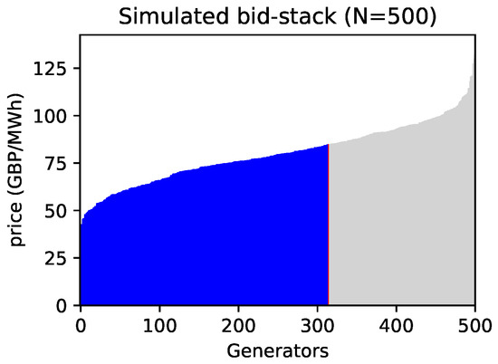
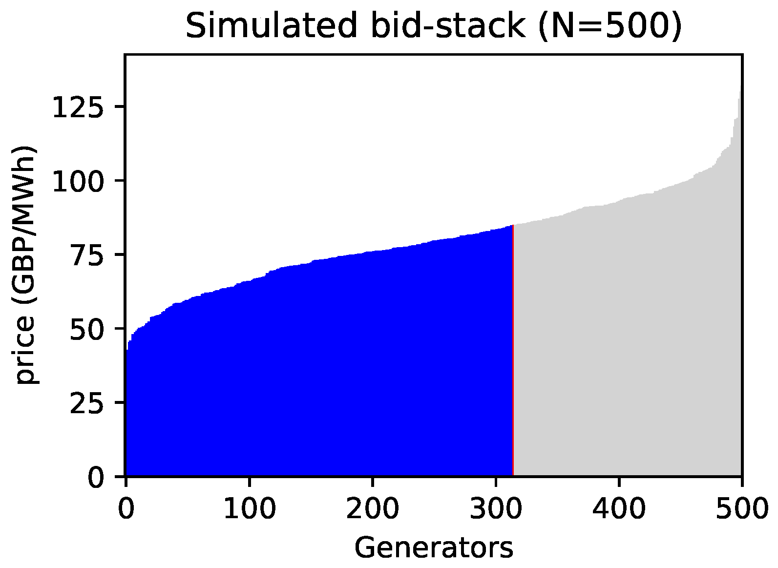
Thus, $q_N\left(t\right)$ is the demand-dependent empirical quantile of the marginal-cost distribution in the finite bid stack. The quantile function will give out the infimum of the marginal cost bids from all generators that match the market demand; we use Figure 1 to show a simple simulated bid stack.

Figure 1. Simulation of a bid stack when $N=500$. Blue bars indicate accepted generators’ bids, gray bars indicate unaccepted bids, and the red vertical line marks the marginal generator and its corresponding market marginal price.

Figure 1 shows a simulated bid stack when $N=500$. By using the quantile function, we can find the market marginal price and corresponding generator, highlighted as a red line in the figure. The blue bars represent accepted and activated generators’ bids; the gray bars represent unaccepted bids.

We introduce an indicator function ${\mathbf{1}}_{\{c_t^i\le q_N\left(t\right)\}}$ to represent that we want to find generators that offer a lower marginal price than the market marginal price at time t, because only in this way can the generator earn a positive operating margin. Hence, the market-clearing payoff component can be defined as

$$F_N^i(c_t^i,{\mu }_t^N)=\left(q_N\left(t\right)-c_t^i\right){\mathbf{1}}_{\{c_t^i\le q_N\left(t\right)\}}$$

(9)

This term is non-local because it depends not only on the individual state $c_t^i$, but also on the empirical distribution ${\mu }_t^N$ through the clearing quantile $q_N\left(t\right)$.

Then, we can define the running payoff of generator i:

$$L_N^i(c_t^i,{\alpha }_t^i,{\mu }_t^N,t)=-{\displaystyle \frac{{\left({\alpha }_t^i\right)}^2}{2}}+F_N^i(c_t^i,{\mu }_t^N)$$

(10)

In the above running payoff function, we use $-{\displaystyle \frac{{\left({\alpha }_t^i\right)}^2}{2}}$ as a penalty term to denote that investment in generator facilities will decrease the profit. To avoid actions like over-investment and malicious competition that may finally break the equilibrium between generators, we give the control term a second order, which means that the penalty on revenue will grow at a square rate if investment in either renewable power or non-renewable power increases too fast and deviates from normal speed.

Finally, the finite-agent objective payoff functional can be defined as follows:

$$J_N^i({\alpha }^1,\dots ,{\alpha }^N)=\mathbb{E}\left[{\int }_0^T{L}_N^i(c_s^i,{\alpha }_s^i,{\mu }_s^N,s)ds+G^i(c_T^i,{\mu }_T^N)\right]$$

(11)

where $G^i$ is the terminal payoff.

Next is the definition for Nash equilibrium in the finite-agent game. We represent the definition in the N-agent situation, and we assume the equilibrium also holds when $N\to \infty$.

Definition 1. 

The point $({\widehat{\alpha }}^1,{\widehat{\alpha }}^2,\dots ,{\widehat{\alpha }}^N)$ is a Nash equilibrium point of the finite-agent game; for every generator i and every admissible alternative control ${\alpha }^i$, we have

$$J_N^i({\widehat{\alpha }}^1,{\widehat{\alpha }}^2,\dots ,{\widehat{\alpha }}^N)\ge J_N^i({\widehat{\alpha }}^1,{\widehat{\alpha }}^2,\dots ,{\widehat{\alpha }}^{i-1},{\alpha }^i,{\widehat{\alpha }}^{i+1},\dots ,{\widehat{\alpha }}^N)$$

This shows that if all controls from agents reach Nash equilibrium, no individual generator can improve its expected payoff by changing its investment strategy, while all other generators keep their equilibrium strategies. In addition, we assume every agent has infinitesimal influence on others.

Another assumption we need is the symmetry property between generators. From the model, we can see that no agent’s cost depends on their own properties or position rank. This means that in any permutation, the value for the cost function should be the same. The symmetry assumption is assumed to hold as $N\to \infty$. This symmetry is important for the mean-field approximation: as N becomes large, the influence of any single generator on the empirical distribution ${\mu }_t^N$ becomes negligible, while the aggregate distribution continues to determine the clearing quantile and hence the market price.

Assumption 2. 

For all permutations σ on $\{1,2,\dots ,N\}$, if we consider a cost function with the form $F_N^i(c^1,c^2,\dots ,c^N)$, the symmetry property means that

$$F_N^{\sigma \left(i\right)}(c^{\sigma \left(1\right)},c^{\sigma \left(2\right)},\dots ,c^{\sigma \left(N\right)})=F_N^i(c^1,c^2,\dots ,c^N)$$

2.2.2. MFG Model

Next, we will derive the mean field game model when $N\to \infty$. The rigorous proof for many cases where $N\to \infty$ is still an open area of research, and only few can be solved. In our case, for convenience in studying the pricing problem, we assume that properties and assumptions under N-agents can transit smoothly to the $N\to \infty$ situation. And addressing this question rigorously would be a question for future research.

We now pass from the finite-agent bid-stack game to its mean-field formulation. The key object in the finite market is the empirical distribution of marginal costs (6). In the mean-field limit, as $N\to \infty$, the effect of any individual generator on the aggregate distribution becomes negligible. We may get the limiting population distribution for ${\mu }_t^N$:

$${\mu }_t^N\Rightarrow {\mu }_t\mathrm{as}N\to \infty$$

(12)

and we introduce $m(c,t)$ as a density: ${\mu }_t\left(dc\right)=m(c,t)dc$.

More precisely, under the symmetry and regularity assumptions stated above, and assuming that the initial marginal costs are independently drawn from a common distribution $m_0$, the empirical distribution ${\mu }_t^N$ is approximated by the population distribution $m_t$ when N is large. Recalling (7), we assume that the cumulative distribution function of $m_t$ is

$$M_t\left(c\right)={\int }_{-\infty }^{c}m(y,t)dy$$

(13)

and $M_t^N\left(c\right)\to M_t\left(c\right)$. Moreover, for each realized demand level $D_t$, assume that the limiting quantile is uniquely determined:

$$q\left(t\right)=Q_{D_t}\left(m_t\right)=inf\{c\in \mathbb{R}:M_t\left(c\right)\ge D_t\}$$

(14)

if $M_t$ is continuous and strictly increasing in a neighborhood of $q\left(t\right)$, then the empirical quantile (8) converges to the limiting clearing quantile $q_N\left(t\right)\to q\left(t\right)$.

This gives a transparent link between the finite-agent game and the mean-field model: the individual generator responds to the market-clearing price, while the clearing price is determined by the population distribution of marginal costs. Next, we will derive the mean field game system.

In the mean-field model, a representative generator has marginal cost dynamics:

$$d{c}_t={\alpha }_{t}dt+\sqrt{2}\sigma d{W}_t$$

(15)

where ${\alpha }_t$ is the generator’s investment control and $W_t$ is standard Brownian motion. The representative generator takes the population distribution $m_t$ as given when solving its individual control problem. The objective functional is

$$J\left(\alpha \right)=\mathbb{E}\left[{\int }_0^{T}L(c_s,{\alpha }_s,m_s,s)ds+G(c_T,m_T)\right]$$

(16)

where the running payoff is

$$L(c_t,{\alpha }_t,m_t,t)=-{\displaystyle \frac{{\alpha }_t^2}{2}}+F(c_t,m_t)$$

(17)

The market-clearing payoff component is

$$F(c_t,m_t)=\left(q\left(t\right)-c_t\right){\mathbf{1}}_{\{c_t\le q\left(t\right)\}}$$

(18)

Let $u(c,t)$ denote the value function of the representative generator:

$$u(c,t)=\underset{\alpha \in \mathcal{A}}{sup}{\mathbb{E}}_{c,t}\left[{\int }_t^T\left(-{\displaystyle \frac{{\alpha }_s^2}{2}}+F(c_s,m_s)\right)ds+G(c_T,m_T)\right]$$

(19)

where ${\mathbb{E}}_{c,t}$ denotes the conditional expectation given $c_t=c$, and the population flow $m_s$ is taken as given by the representative generator. Next, we will use the dynamic programming principle to derive the HJB equation.

Theorem 1 

(Dynamic programming principle). Consider a finite-horizon stochastic control problem on $[0,T]$ with a controlled state process:

$$d{X}_s=b(s,X_s,{\alpha }_s)ds+\sigma (s,X_s,{\alpha }_s)d{W}_s,X_t=x$$

(20)

where $\alpha \in {\mathcal{A}}_{t,T}$ is an admissible control. Let the value function be

$$u(x,t)=\underset{\alpha \in {\mathcal{A}}_{t,T}}{sup}{\mathbb{E}}_{x,t}\left[{\int }_t^{T}f(s,X_s,{\alpha }_s)ds+g\left(X_T\right)\right]$$

(21)

Assume that the controlled state equation is well posed and that f and g satisfy the standard regularity and growth conditions under which the value function is finite. Then, for any deterministic time $r\in [t,T]$,

$$u(x,t)=\underset{\alpha \in {\mathcal{A}}_{t,r}}{sup}{\mathbb{E}}_{x,t}\left[{\int }_t^{r}f(s,X_s,{\alpha }_s)ds+u(X_r,r)\right]$$

(22)

In particular, for any $h>0$ such that $t+h\le T$,

$$u(x,t)=\underset{\alpha \in {\mathcal{A}}_{t,t+h}}{sup}{\mathbb{E}}_{x,t}\left[{\int }_t^{t+h}f(s,X_s,{\alpha }_s)ds+u(X_{t+h},t+h)\right]$$

(23)

We now apply the dynamic programming principle to the representative generator’s control problem. The value function is

$$u(c,t)=\underset{\alpha \in {\mathcal{A}}_{t,T}}{sup}{\mathbb{E}}_{c,t}\left[{\int }_t^T\left(-{\displaystyle \frac{{\alpha }_s^2}{2}}+F(c_s,m_s)\right)ds+G(c_T,m_T)\right]$$

(24)

By the dynamic programming principle, for any small $h>0$,

$$u(c,t)=\underset{\alpha \in {\mathcal{A}}_{t,t+h}}{sup}{\mathbb{E}}_{c,t}\left[{\int }_t^{t+h}\left(-{\displaystyle \frac{{\alpha }_s^2}{2}}+F(c_s,m_s)\right)ds+u(c_{t+h},t+h)\right]$$

(25)

Assume that u is sufficiently smooth. Applying Itô’s formula to $u(c_s,s)$ gives

$$du(c_s,s)=\left(u_t(c_s,s)+{\alpha }_s{D}_{c}u+{\sigma }^2{D}_{cc}u\right)ds+\sqrt{2}\sigma D_{c}ud{W}_s$$

(26)

Integrating from t to $t+h$ and taking the conditional expectation yields

$${\mathbb{E}}_{c,t}\left[u(c_{t+h},t+h)-u(c,t)\right]={\mathbb{E}}_{c,t}\left[{\int }_t^{t+h}\left(u_s+{\alpha }_s{D}_{c}u+{\sigma }^2{D}_{cc}u\right)ds\right]$$

(27)

Substituting this into the DPP gives

$$0=\underset{\alpha \in {\mathcal{A}}_{t,t+h}}{sup}{\mathbb{E}}_{c,t}\left[{\int }_t^{t+h}\left(u_s+{\alpha }_s{D}_{c}u+{\sigma }^2{D}_{cc}u-{\displaystyle \frac{{\alpha }_s^2}{2}}+F(c_s,m_s)\right)ds\right]$$

(28)

Dividing by h and letting $h\to 0$, we obtain

$$0=\underset{\alpha \in \mathcal{A}}{sup}\left\{u_t+\alpha D_{c}u+{\sigma }^2{D}_{cc}u-{\displaystyle \frac{{\alpha }^2}{2}}+F(c,m_t)\right\}$$

(29)

Equivalently,

$$-u_t-{\sigma }^2{D}_{cc}u-\underset{\alpha \in \mathcal{A}}{sup}\left\{\alpha D_{c}u-{\displaystyle \frac{{\alpha }^2}{2}}\right\}=F(c,m_t)$$

(30)

Define the Hamiltonian by

$$H\left(p\right)=\underset{\alpha \in \mathcal{A}}{sup}\left\{\alpha p-{\displaystyle \frac{{\alpha }^2}{2}}\right\}$$

(31)

If $\mathcal{A}=\mathbb{R}$, then we have

$$H\left(p\right)={\displaystyle \frac{1}{2}}{\left|p\right|}^2,{\alpha }^{*}(c,t)=D_{p}H\left(D_{c}u(c,t)\right)=D_{c}u(c,t)$$

(32)

Substituting the optimal control (32) into (30) yields the Hamilton–Jacobi equation

$$\left\{\begin{array}{c}-u_t-{\sigma }^2{D}_{cc}u-{\displaystyle \frac{1}{2}}{\left|D_{c}u\right|}^2=F(c,m_t)\hfill \\ u(c,T)=G(c,m_T)\hfill \end{array}\right.$$

(33)

Given the optimal feedback control ${\alpha }^{*}(c,t)$, the population density of marginal costs evolves according to the Fokker–Planck equation:

$$\left\{\begin{array}{c}{m}_t-{\sigma }^2{D}_{cc}m+D_c\left(m{\alpha }^{*}(c,t)\right)=0\hfill \\ m(c,0)=m_0\left(c\right)\hfill \end{array}\right.$$

(34)

Using (32), the coupled mean-field game system becomes

$$\left\{\begin{array}{c}-u_t-{\sigma }^2{D}_{cc}u-{\displaystyle \frac{1}{2}}{\left|D_{c}u\right|}^2=F(c,m_t)\hfill \\ m_t-{\sigma }^2{D}_{cc}m+D_c\left(m{D}_{c}u\right)=0\hfill \\ m(c,0)=m_0\left(c\right),u(c,T)=G(c,m_T)\hfill \end{array}\right.$$

(35)

3. Simulation

This section presents the numerical simulation component of the one-dimensional MFG electricity-pricing model. The purpose is to show how the theoretical bid-stack mechanism behaves when demand is calibrated from observed electricity-market data.

3.1. Data Process

The demand data are the National Energy System Operator (NESO) Historic Demand Data from 1 January 2023 to 31 December 2025 [27,28,29]. The NESO files report national demand for each half-hour settlement period with demand measured in MW. We exclude all non-finite, non-positive or missing observations. And for the calibration, the half-hourly MW observations are aggregated into daily electricity demand by summing the 48 settlement-period values and multiplying by 0.5, so that the resulting unit is MWh/day. Days with daylight-saving-time adjustment contain 46 or 50 settlement periods; these days are retained and aggregated using their actual number of settlement periods. We get 1096 daily observations in the demand series in MWh/day after aggregation, and we use the min–max standardized method to normalize data.

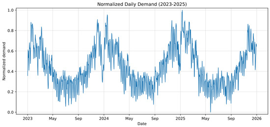
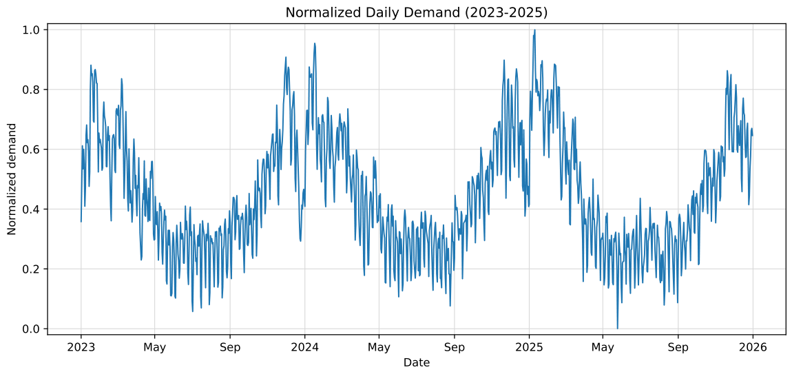
The standardized NESO demand is shown in Figure 2. The process exhibits a clear seasonal pattern over 2023–2025. Demand is higher during winter months and lower during late spring and summer, indicating a stable annual cycle in electricity consumption. Around this time-varying seasonal level, short-run fluctuations tend to dissipate rather than drift permanently, as local peaks and troughs are followed by movements back toward the seasonal band. This combination of seasonality and mean-reverting behavior supports the use of a seasonal mean-reverting demand process in the simulation.

Figure 2. Standardized demand data.

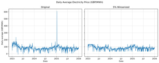
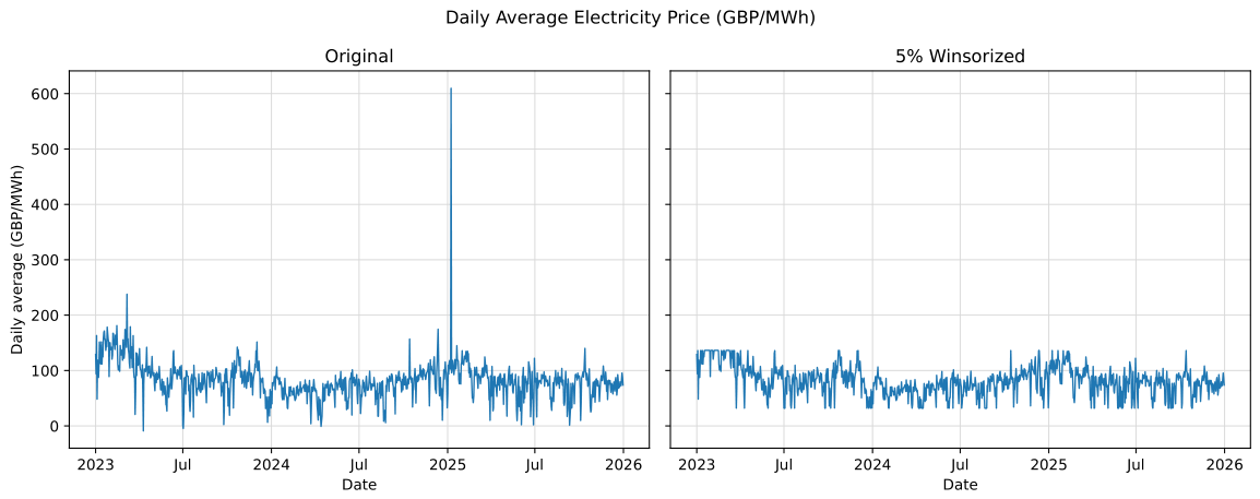
The price data are taken from the Office for National Statistics System Price of electricity series, which is used as an empirical proxy for the observed spot-price level [30]. We use the daily average system-price observations from 1 January 2023 to 31 December 2025, matching the demand sample period. We drop all missing or non-finite observations, and convert the unit of the price from p/KWh to GBP/MWh. Because electricity prices may contain short-lived scarcity spikes and extreme observations, we apply a 5% winsorization before it is used for parameter estimation. The processed price series is shown in Figure 3.

Figure 3. Daily average electricity price.

3.2. Numerical Simulation

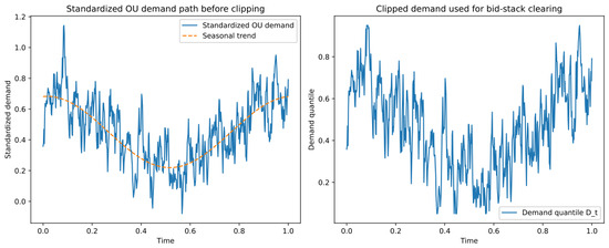
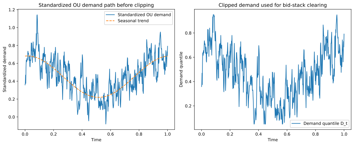
The demand process follows the seasonal mean-reverting specification introduced in Section 2.1. Following the calibration strategy in [11], the parameters $(s_0,s_1,s_2,{\mu }_d,{\sigma }_d)$ are estimated from the three-year daily demand series by the exact Gaussian maximum likelihood. The baseline demand parameters used in the solver are reported in Appendix A. The simulated demand quantile is clipped to the interval $[0.05,0.95]$ in order to avoid numerical instability at the two extreme tails of the cost distribution. Figure 4 reports this construction in unit time. The left panel gives the standardized seasonal OU demand path before clipping, together with its deterministic seasonal trend. The right panel gives the clipped demand series used as the demand quantile $D_t$. Thus, $D_t$ is interpreted as the fraction of the bid stack that must be activated; for example, $D_t=0.6$ means that roughly the lowest-cost 60% of bids are activated.

Figure 4. Simulated demand path used as the demand quantile $D_t$ in the bid-stack clearing rule.

The processed price series is used to calibrate the initial mean and variance of the marginal-cost distribution $c_0$ in the simulation. After winsorizing the observed system-price series, we estimate its empirical mean and variance using the normal maximum-likelihood estimator; the calibrated values can be found in Appendix A. In the baseline calibration, we set $c_{\mathrm{fixed}}=5$ GBP/MWh. The sensitivity of the simulation results to this fixed bid-price component is reported separately in Appendix B.

The numerical scheme solves the equations by Picard fixed-point iteration. At the two cost boundaries, we impose homogeneous Neumann conditions for the value function. For the density equation, we impose a no-flux condition at both boundaries so that probability mass is conserved over the truncated computational domain. After each forward step, the density is renormalized to integrate to one. The parameter setting can be found in Appendix A. At each iteration, the demand-dependent clearing quantile $q\left(t\right)=Q_{D_t}\left(m_t\right)$ is computed from the current marginal-cost distribution. Inspired by [31], we estimate the indicator function in the bid-stack payoff (18) through a smoothed logistic function to improve the stability:

$${\pi }_{\epsilon }(c,q)={\displaystyle \frac{1}{1+exp\left(\right(c-q)/\epsilon )}}$$

(36)

The parameter $\epsilon >0$ controls the width of the transition region around the clearing margin. In the baseline simulation we set $\epsilon =1.5$ to prevent small changes in the clearing quantile from generating discrete jumps in the payoff; the sensitivity check is shown in Appendix B.

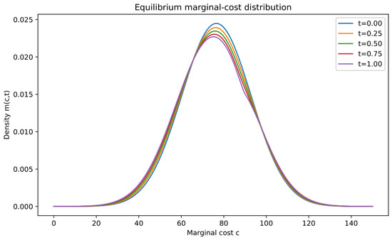
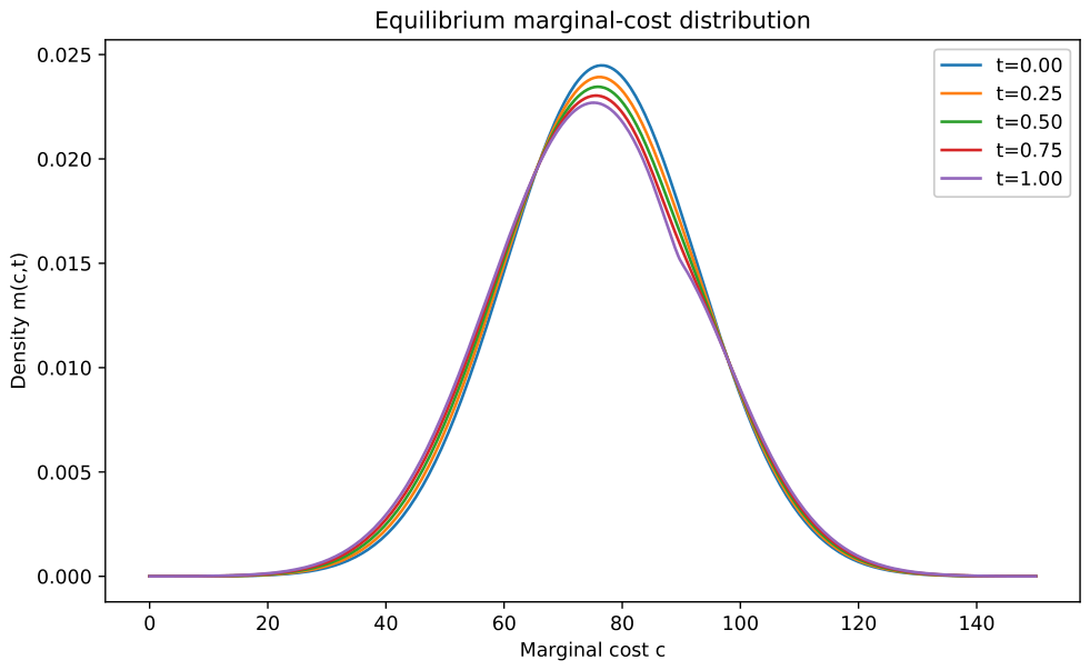
Figure 5 shows the resulting equilibrium marginal-cost distribution in unit time. Several features are worth noting. First, over the simulation horizon, the mean of the distribution moves to the left. This downward movement reflects the aggregate effect of cost-reduction incentives, which are interpreted as renewable-oriented investment. This is the key endogenous channel in the model: when generators reduce marginal costs, the distribution $m_t$ changes, and because the clearing price depends on the demand quantile $Q_{D_t}\left(m_t\right)$, the price-formation mechanism changes with the equilibrium cost distribution rather than being imposed as an exogenous price path.

Figure 5. Evolution of the equilibrium marginal-cost distribution at selected time points.

Second, the peak of the density becomes lower and dispersed over time, indicating that the transition effect is heterogeneous across generators. Some producers move toward lower marginal costs, while others remain in relatively high-cost regions. This dispersion is important because it shows that the market does not induce a uniform cost reduction for all firms.

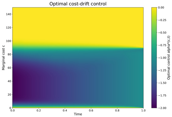
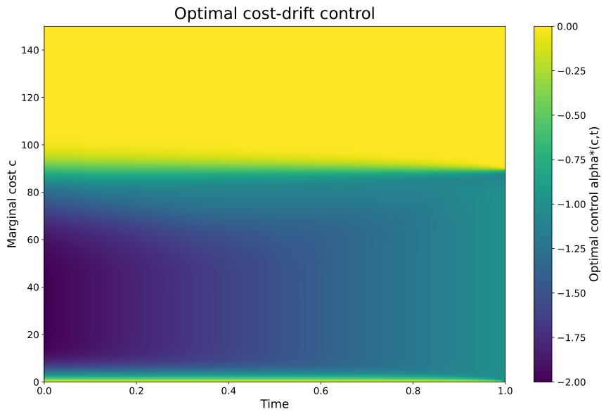
Figure 6 shows that the optimal control differs across cost and price regions. Negative values of ${\alpha }^{*}(c,t)$ represent marginal-cost reduction in the model, which is interpreted as renewable-oriented investment, technical upgrading, or other cost-reduction efforts. The heatmap indicates that these incentives are not uniform. The strongest negative controls occur for generators that are already competitive or close to the clearing region, while high-cost generators receive much weaker private incentives to reduce costs.

Figure 6. Optimal cost-drift control ${\alpha }^{*}(c,t)$ over time and marginal-cost states. Negative values represent marginal-cost reduction incentives.

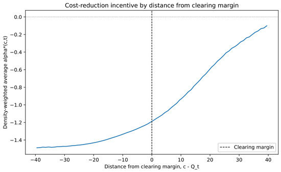
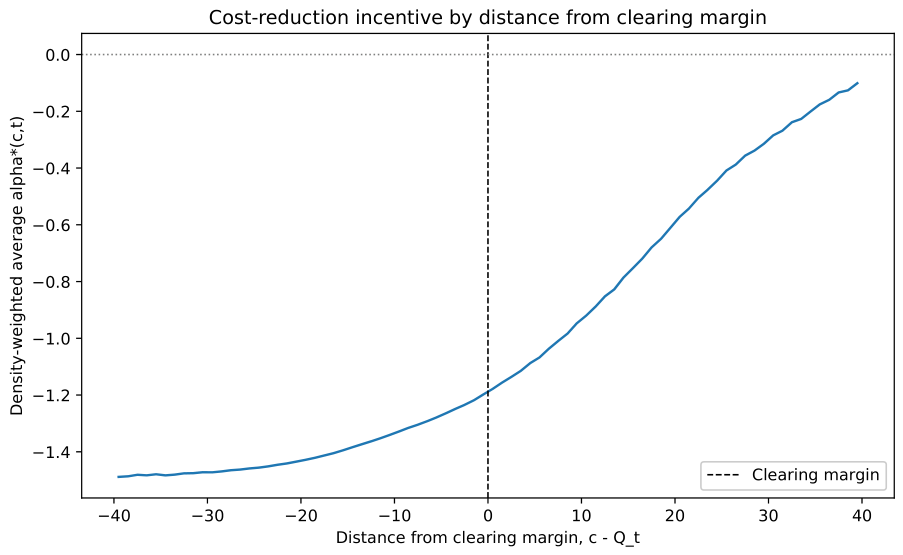
Figure 7 further supports this conclusion by plotting the density-weighted average optimal control against the distance from the clearing margin, $c-Q_{D_t}\left(m_t\right)$. A positive distance means that the generator’s cost is above the clearing margin, while a negative distance means that the generator is inside the active bid-stack region. The cost-reduction incentive becomes weak when $c-Q_{D_t}\left(m_t\right)>0$, and it is stronger when the generator is already below or near the clearing margin. This pattern is important for sustainability policy: market competition rewards generators that are already competitive or close to becoming competitive, but high-cost generators far above the clearing margin may have limited self-driven incentives to undertake costly low-carbon transition.

Figure 7. Density-weighted average optimal control by distance from the clearing margin $c-Q_{D_t}\left(m_t\right)$. The blue line plots the density-weighted average optimal control. The horizontal black dotted line marks zero control, and the vertical black dotted line marks the clearing margin.

Overall, the numerical simulation illustrates the mechanism between renewable-oriented cost reduction, bid-stack clearing, and heterogeneous investment incentives. As shown by the evolution of the marginal-cost density, cost-reduction investment lowers the average marginal cost of the generators, but the widening of the distribution also indicates that this transition effect is not uniform across firms. Some generators move more strongly toward lower-cost regions, whereas others remain in relatively high-cost states.

The optimal-control results further show why this heterogeneity arises. Generators that are already below or close to the clearing margin have stronger incentives to reduce costs, because additional cost reduction increases their probability of being dispatched and improves their margin relative to the market-clearing price. By contrast, generators far above the clearing margin face weaker private incentives, since moderate cost reductions may still be insufficient in bringing them into the active bid-stack region. Therefore, within the model, market competition can promote renewable-oriented cost reduction among competitive or near-competitive producers, but it may not be sufficient in inducing a system-wide low-carbon transition. This provides an economic rationale for complementary policy instruments, such as transition subsidies, tax incentives, or green finance, targeted especially at high-cost generators with weak market-based transition incentives.

4. Conclusions

This study develops an electricity pricing model based on a second-order mean field game with a non-local bid-stack payoff. The model links generators’ renewable-oriented investment decisions to the controlled drift of marginal generation costs and embeds the resulting cost distribution into a bid-stack clearing mechanism. In this setting, the market-clearing price is determined by a demand-dependent quantile of the population marginal-cost distribution. The analysis therefore connects individual cost-reduction incentives, the evolution of the generator population, and market-level price formation within a unified framework.

The simulations show that renewable-oriented cost reduction can shift the equilibrium cost distribution toward lower-cost regions. However, the transition effect is heterogeneous across firms. The optimal-control results further show that generators already below or close to the clearing margin have stronger incentives to reduce costs, because additional cost reduction increases their probability of dispatch and improves their margin. By contrast, generators far above the clearing margin face weaker private incentives, since moderate cost reductions may still be insufficient in bringing them into the active bid-stack region. These findings have implications for sustainable electricity-market design. Market competition can support renewable-oriented cost reduction among competitive generators, but it may not provide sufficient incentives for high-cost generators that remain far from dispatch. Therefore, complementary policy instruments may be needed to help correct the gap faced by high-cost generators.

References

- Agency, I.R.E. Renewable Power Generation Costs in 2021; International Renewable Energy Agency: Abu Dhabi, United Arab Emirates, 2022. [Google Scholar]
- Marrero, G.A.; Ramos-Real, F.J. Electricity generation cost in isolated system: The complementarities of natural gas and renewables in the Canary Islands. Renew. Sustain. Energy Rev. 2010, 14, 2808–2818. [Google Scholar] [CrossRef] [Scilit]
- Sims, R.E.; Rogner, H.H.; Gregory, K. Carbon emission and mitigation cost comparisons between fossil fuel, nuclear and renewable energy resources for electricity generation. Energy Policy 2003, 31, 1315–1326. [Google Scholar] [CrossRef] [Scilit]
- Brown, T.; Reichenberg, L. Decreasing market value of variable renewables can be avoided by policy action. Energy Econ. 2021, 100, 105354. [Google Scholar] [CrossRef] [Scilit]
- Liebensteiner, M.; Naumann, F. Can carbon pricing counteract renewable energies’ cannibalization problem? Energy Econ. 2022, 115, 106345. [Google Scholar] [CrossRef] [Scilit]
- Antweiler, W.; Muesgens, F. On the long-term merit order effect of renewable energies. Energy Econ. 2021, 99, 105275. [Google Scholar] [CrossRef] [Scilit]
- Biggar, D.R.; Hesamzadeh, M.R. The Economics of Electricity Markets; Wiley Blackwell: Hoboken, NJ, USA, 2014. [Google Scholar]
- Harris, C. Electricity Markets: Pricing, Structures and Economics; John Wiley & Sons: Hoboken, NJ, USA, 2006; Volume 328. [Google Scholar]
- Schweppe, F.C.; Caramanis, M.C.; Tabors, R.D.; Bohn, R.E. Spot Pricing of Electricity; Springer Science & Business Media: Berlin/Heidelberg, Germany, 2013. [Google Scholar]
- Barlow, M.T. A diffusion model for electricity prices. Math. Financ. 2002, 12, 287–298. [Google Scholar] [CrossRef] [Scilit]
- Aïd, R.; Campi, L.; Huu, A.N.; Touzi, N. A structural risk-neutral model of electricity prices. Int. J. Theor. Appl. Financ. 2009, 12, 925–947. [Google Scholar] [CrossRef] [Scilit]
- Aïd, R.; Campi, L.; Langrené, N. A Structural Risk-Neutral Model for Pricing and Hedging Power Derivatives. Math. Financ. Int. J. Math. Stat. Financ. Econ. 2013, 23, 387–438. [Google Scholar]
- Böttger, D.; Härtel, P. On wholesale electricity prices and market values in a carbon-neutral energy system. Energy Econ. 2022, 106, 105709. [Google Scholar] [CrossRef] [Scilit]
- Newbery, D.M. Estimating the target-consistent carbon price for electricity. Energy J. 2025, 46, 25–43. [Google Scholar]
- Abrell, J.; Rausch, S.; Streitberger, C. The economic and climate value of flexibility in green energy markets. Environ. Resour. Econ. 2022, 83, 289–312. [Google Scholar]
- Villavicencio, M.; Finon, D. The Social Efficiency of Electricity Transition Policies Based on Renewables. Which Ways of Improvement? Energy J. 2022, 43, 195–216. [Google Scholar] [CrossRef] [Scilit]
- Bohland, M.; Schwenen, S. Renewable support and strategic pricing in electricity markets. Int. J. Ind. Organ. 2022, 80, 102792. [Google Scholar] [CrossRef] [Scilit]
- Sirin, S.M.; Uz, D.; Sevindik, I. How do variable renewable energy technologies affect firm-level day-ahead output decisions: Evidence from the Turkish wholesale electricity market. Energy Econ. 2022, 112, 106169. [Google Scholar] [CrossRef] [Scilit]
- Lasry, J.M.; Lions, P.L. Jeux à champ moyen. I—Le cas stationnaire. Comptes Rendus Math. 2006, 343, 619–625. [Google Scholar] [CrossRef] [Scilit]
- Lasry, J.M.; Lions, P.L. Jeux à champ moyen. II—Horizon fini et contrôle optimal. Comptes Rendus Math. 2006, 343, 679–684. [Google Scholar] [CrossRef] [Scilit]
- Lasry, J.M.; Lions, P.L. Mean field games. Jpn. J. Math. 2007, 2, 229–260. [Google Scholar] [CrossRef] [Scilit]
- Huang, M.; Malhamé, R.P.; Caines, P.E. Large population stochastic dynamic games: Closed-loop McKean-Vlasov systems and the Nash certainty equivalence principle. Commun. Inf. Syst. 2006, 6, 221–252. [Google Scholar] [CrossRef] [Scilit]
- Kizilkale, A.C.; Malhame, R.P. Collective target tracking mean field control for markovian jump-driven models of electric water heating loads. IFAC Proc. Vol. 2014, 47, 1867–1872. [Google Scholar] [CrossRef] [Scilit]
- Carmona, R.; Dayanıklı, G.; Laurière, M. Mean Field Models to Regulate Carbon Emissions in Electricity Production. Dyn. Games Appl. 2022, 12, 897–928. [Google Scholar] [CrossRef] [Scilit]
- Shrivats, A.V.; Firoozi, D.; Jaimungal, S. A mean-field game approach to equilibrium pricing in solar renewable energy certificate markets. Math. Financ. 2022, 32, 779–824. [Google Scholar] [CrossRef] [Scilit]
- Do, L.P.C.; Lyócsa, Š.; Molnár, P. Residual electricity demand: An empirical investigation. Appl. Energy 2021, 283, 116298. [Google Scholar] [CrossRef] [Scilit]
- National Energy System Operator. Historic Demand Data 2023. 2023. Available online: https://www.neso.energy/data-portal/historic-demand-data/historic_demand_data_2023 (accessed on 20 May 2026).
- National Energy System Operator. Historic Demand Data 2024. 2024. Available online: https://www.neso.energy/data-portal/historic-demand-data/historic_demand_data_2024 (accessed on 20 May 2026).
- National Energy System Operator. Historic Demand Data 2025. 2025. Available online: https://www.neso.energy/data-portal/historic-demand-data/historic_demand_data_2025 (accessed on 20 May 2026).
- Office for National Statistics. System Price of Electricity. 2026. Available online: https://www.ons.gov.uk/economy/economicoutputandproductivity/output/datasets/systempriceofelectricity/2026 (accessed on 20 May 2026).
- He, X.; Pan, X.; Tan, K.M.; Zhou, W.X. Smoothed quantile regression with large-scale inference. J. Econom. 2023, 232, 367–388. [Google Scholar] [CrossRef] [Scilit]
Disclaimer/Publisher’s Note: The statements, opinions and data contained in all publications are solely those of the individual author(s) and contributor(s) and not of MDPI and/or the editor(s). MDPI and/or the editor(s) disclaim responsibility for any injury to people or property resulting from any ideas, methods, instructions or products referred to in the content. |
© 2026 by the authors. Licensee MDPI, Basel, Switzerland. This article is an open access article distributed under the terms and conditions of the Creative Commons Attribution (CC BY) license.