Spatiotemporal Patterns and Influencing Factors of Agricultural Eco-Efficiency in the Yangtze River Economic Belt

Abstract

In the context of global climate change and intensifying resource and environmental constraints, improving agricultural eco-efficiency (AEE) has become critical to achieving the green transformation of agriculture. This study develops a comprehensive evaluation index system for AEE that incorporates factor inputs, expected outputs, and undesirable outputs. Using county-level panel data from 2010 to 2022 for the Yangtze River Economic Belt (YEB), it applied the super-efficiency slacks-based measure (SBM) model to quantify AEE. Furthermore, spatial autocorrelation analysis and the spatial Durbin model (SDM) are employed to reveal its spatiotemporal characteristics and influencing factors of AEE. The results indicate that the overall AEE of the YEB exhibited a fluctuating upward trend over the study period, yet significant regional heterogeneity persisted. AEE showed pronounced positive spatial correlations, with regional disparities primarily stemming from hyper-variance intensity, suggesting that high- and low-efficiency counties are spatially interwoven. The SDM results indicate that local temperature, economic development, urbanization, fiscal support for agriculture, and agricultural production structure positively influence local AEE, while rural residents’ income and educational attainment exert negative effects. These factors also demonstrate significant spatial spillover effects, with economic development and ecological conditions in adjacent regions generating positive externalities, while neighboring urbanization and temperature producing negative impacts. This study deepens the understanding of the driving mechanisms underlying AEE from a spatial interdependence perspective, providing a scientific basis for formulating cross-regional collaborative policies aimed at promoting green agricultural development in major river basins.

1. Introduction

In the context of global climate change and increasingly stringent resource and environmental constraints, achieving sustainable agricultural development has become a global issue [1,2]. The traditional high-input, high-output agricultural production model, while ensuring food security, has also led to a series of severe ecological and environmental problems, including excessive resource consumption, intensified non-point source pollution, and ecosystem degradation [3,4,5]. Consequently, enhancing agricultural eco-efficiency (AEE), i.e., producing more agricultural products with fewer resource inputs and less environmental pollution, has emerged as the core pathway to reconciling the dilemma between agricultural development and environmental protection [5]. As the world’s largest agricultural nation, China’s pursuit of green and low-carbon agricultural development carries profound implications for the realization of global sustainable development.

The Yangtze River Economic Belt (YEB), a major strategic region spanning eastern, central, and western China, serves not only as the core axis of national socioeconomic development but also as a crucial area for ensuring national food and ecological security [6,7]. Agriculture plays a dual role in regional development, functioning both as a foundation sector and a strategic pillar. For a long time, the traditional agricultural production model, driven by factor inputs and resource consumption, has supported economic growth and social supply [8]. However, it has also led to a series of resource and environmental issues [6,7,9], placing persistent pressure on the ecological environment of the Yangtze River basin. To address this, the government has established “ecological priority and green development” as the core principle guiding the development of the YEB. Accordingly, scientifically evaluating the AEE of the YEB, revealing its spatiotemporal patterns, and accurately identifying its driving and constraining factors not only actively responds to major national strategies but also constitutes an intrinsic requirement for exploring sustainable agricultural development in major river basins. This endeavor holds significant theoretical value and practical urgency.

AEE, as a key indicator for assessing the economic and ecological benefits of agricultural production [5,10], has garnered extensive scholarly attention worldwide, yielding a rich body of research. In terms of measurement methods, Data Envelopment Analysis (DEA) and its extensions, such as the Slacks-Based Measure (SBM) model that accounts for undesirable outputs, are widely adopted due to their advantages in handling issues about multi-input and multi-output [11,12,13]. Regarding research scale, existing studies predominantly focus on national, provincial, or prefectural levels [11,12,14], with relatively limited attention given to the more granular county-level scale. In terms of spatiotemporal pattern analysis, most studies reveal significant regional disparities and spatial clustering characteristics in AEE [15,16]. Nevertheless, in-depth analysis of the long-term spatiotemporal evolution and spatial dependency effects of AEE at the county level within the YEB remains relatively weak. As for the exploration of influencing factors, existing research has identified the roles of multiple factors such as economic development, industrial structure, technological progress, environmental regulations, and resource endowments in the evolution of AEE [5,14,15,16]. However, most studies employ ordinary panel regression models [5], which fail to adequately account for the inherent spatial interdependence of agricultural activities, potentially leading to estimation biases. The introduction of spatial econometrics provides a more suitable tool for revealing the spatial interactions among these factors.

In summary, while existing research has laid a solid foundation for understanding AEE, several areas remain open for further exploration. First, an indicator system more closely aligned with the complex “resource–economy–environment” characteristics of agriculture in the YEB should be established, and the super-efficiency model should be applied to enhance discriminatory power and accuracy. Second, long-term studies at the county level needs to be strengthened to reveal more detailed spatiotemporal patterns of AEE evolution. Third, spatial effects should be incorporated, using spatial econometric models to analyze the influencing factors of AEE and its spatial interaction mechanisms.

This study takes the YEB as its research area and counties as its spatial unit. By constructing a comprehensive evaluation index system for AEE that incorporates factor inputs, expected outputs, undesirable outputs, and by applying a super-efficiency SBM model, this study calculates the AEE for each county in the YEB from 2010 to 2022, revealing their spatiotemporal characteristics. A spatial econometric model is then constructed to empirically examine the natural and human factors influencing AEE, along with their potential spatial spillover effects. Relative to prior AEE studies, this study offers four distinctive contributions: ① a county-level scale that enables more refined spatial analysis; ② a long study window spanning from 2010 to 2022 to capture recent policy-driven dynamics; ③ an integrated evaluation framework that explicitly incorporates undesirable outputs to reflect the environmental costs of agricultural production; and ④ a systematic spatial spillover analysis that moves beyond conventional non-spatial models to uncover interregional interaction mechanisms. Together, these contributions provide new empirical evidence for deepening the understanding of spatiotemporal patterns of sustainable agricultural development in the YEB through more refined measurements, dynamic pattern analysis, and factor detection from a spatial association perspective. This study also seeks to offer scientific basis and decision-making references for promoting regional agricultural green transformation and collaborative governance.

2. Materials and Methods

2.1. Study Area

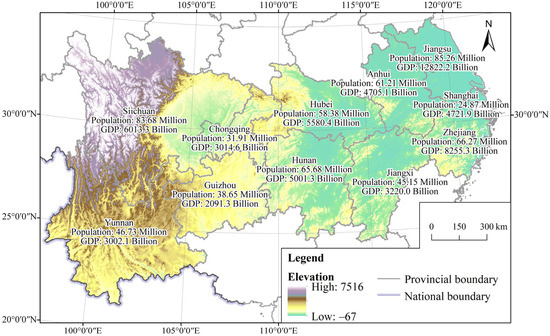
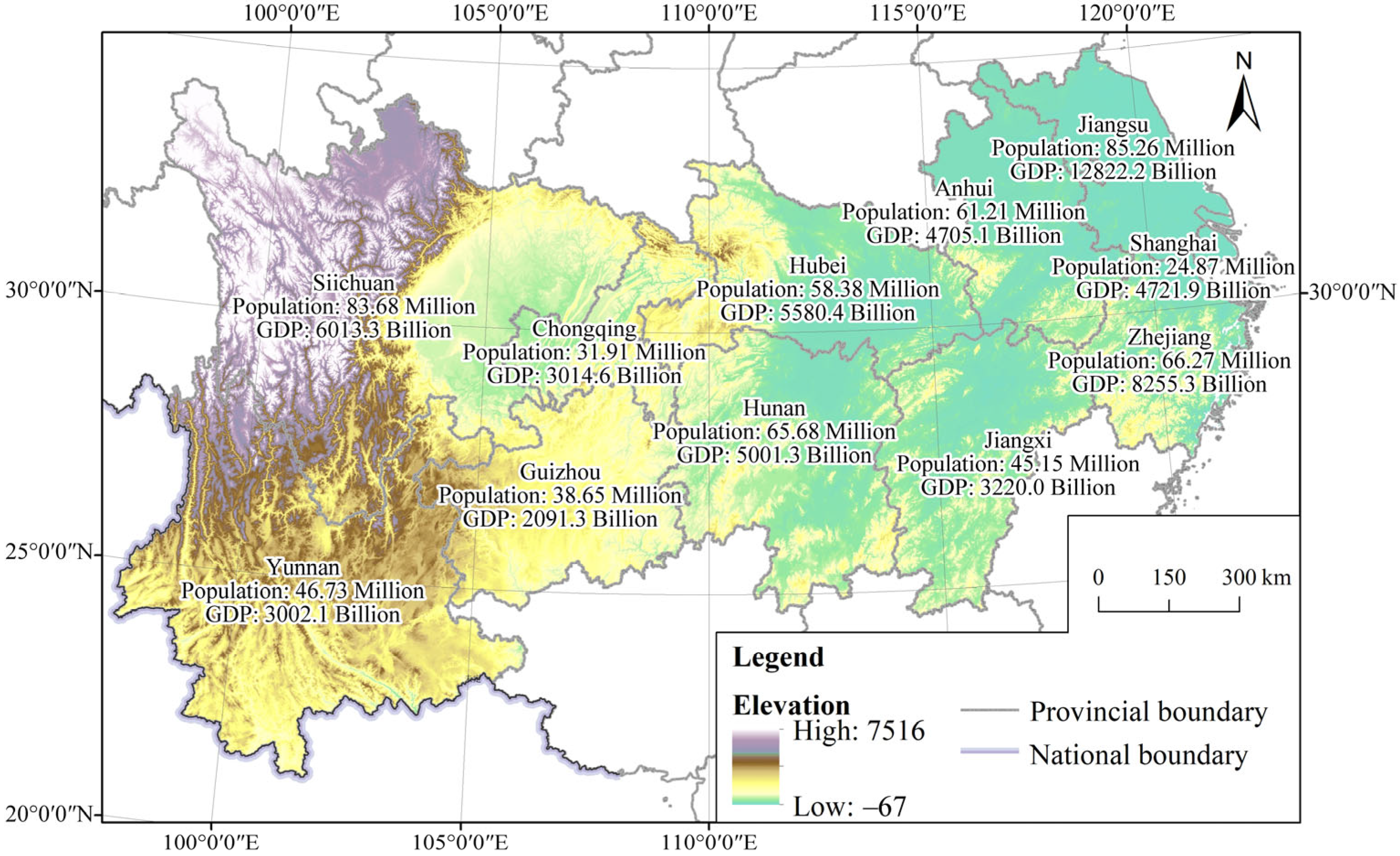
The YEB encompasses 11 provincial-level administrative divisions, including Shanghai, Jiangsu, Zhejiang, Anhui, Jiangxi, Hubei, Hunan, Chongqing, Sichuan, Yunnan, and Guizhou. It covers a land area of approximately 2.05 million km², accounting for 21.4% of China’s total land area and spanning latitudes from approximately 21°8′ N to 35°20′ N and longitudes from 97°21′ E to 123°10′ E. This region accounts for half of the nation’s population and economic output, holding a pivotal strategic position in China’s overall development landscape (Figure 1). In 2023, the shares of value-added from the primary, secondary, and tertiary sectors in the gross regional product changed from 9.22%, 49.70%, and 41.08% in 2010 to 6.57%, 38.45%, and 54.98%, respectively. Meanwhile, the YEB is endowed with abundant and diverse agricultural climate resources. From the alluvial plains in the lower reaches to the hilly basins in the middle reaches and the plateau and mountainous in the upper reaches, the region has developed complex and varied agricultural production systems. As a major production area and supply base for grain, oilseeds, freshwater products, and specialty agricultural products in China, the YEB plays a crucial role in ensuring national food security and the supply of agricultural products [6,7]. However, the region also faces severe challenges such as agricultural non-point source pollution and ecological degradation, which have led to prominent sustainability issues.

Figure 1. Overview of the Yangtze River Economic Belt. The population and GDP data in the chart were based on 2023 statistics.

Agricultural development along the YEB has long exhibited significant regional variations and functional differentiation. The downstream region features a developed economies with high capital and technology intensity but faces tight arable land resources and stringent ecological constraints. The midstream region constitutes China’s traditional grain-producing heartland, characterized by intensive agricultural practices, heavy fertilizer and pesticide inputs, and mounting ecological pressures. The upstream region, with its complex terrain, fragile ecosystems, and relatively extensive agricultural development, struggles with intertwined problems such as soil erosion and desertification [17,18]. Meanwhile, advancing ecological priority and green development in the YEB has become a major national strategic direction, imposing higher demands on the green transformation of agriculture [8]. Therefore, systematically evaluating the spatiotemporal patterns of AEE at the county level and thoroughly exploring its driving mechanisms holds urgent practical significance for synergistically advancing high-quality regional development.

2.2. Evaluation Indicator System

Agricultural production efficiency and AEE serve as crucial indicators for assessing sustainable agricultural development. The former primarily focuses on how the allocation of various factors within agricultural production processes affects economic output [19]. The latter emphasizes the coordination between agricultural production and the ecological environment, attending not only to economic output but also to the negative impacts of agricultural production on natural systems [5]. Although no consensus has been reached on the definition of AEE, a common understanding has emerged regarding its core: achieving the maximum agricultural economic output that meets societal needs with minimal resource consumption and minimal environmental pressure [5,10]. Evidently, AEE transcends the traditional framework for evaluating agricultural productivity. By incorporating resource and environmental costs into performance accounting systems, it reflects the coupling and coordination between human and natural subsystems within agriculture.

From a theoretical perspective, a scientific and comprehensive AEE evaluation index system must encompass three dimensions of factor inputs, expected outputs, and unexpected outputs to fully characterize the triple bottom line balance among resources, economy, and environment. Following the principles of systematicity, representativeness, and data availability, as well as drawing upon existing research [5,10,20,21], this study establishes an evaluation index system for AEE at the county level within the YEB (Table 1). Specifically, factor inputs reflect the various resources occupied and consumed in agricultural production, including land, labor, water resources, energy, and others. Expected outputs refer to the benefits provided by agricultural systems, typically measured by indicators such as agricultural output value and food production. Undesirable outputs refer to various emissions and disturbances generated during agricultural production that negatively impact ecosystems, such as greenhouse gases, nitrogen and phosphorus runoff, and pesticide residues.

Table 1. Evaluation indicator system for AEE.

Dimension	Indicator	Definition
Factor inputs	Land	Total sown areas of farm crops (Hectares)
	Labor	Number of rural primary sector employees (Person)
	Water resources	Effective irrigated area of cultivated land (Hectares)
	Fertilizers	Consumption of chemical fertilizers (Pure nutrient equivalent) (Tons)
	Pesticides	Consumption of pesticides (Pure nutrient equivalent) (Tons)
	Agricultural film	Usage of agricultural film (Tons)
	Machinery	Total power of agricultural machinery (10,000 kW)
	Energy	Electricity consumed in rural areas (10,000 kWh)
Expected outputs	Economic benefits	Gross output value of agriculture, forestry, animal husbandry and fishery (10,000 Yuan)
	Social Benefits	Grain production (Tons)
Undesirable outputs	Environmental impact	Agricultural carbon emissions (Tons): Total carbon emissions calculated using the coefficient method, including chemical fertilizers, pesticides, plastic film, agricultural irrigation, and agricultural tillage [22,23].
		Agricultural nonpoint source pollution: Calculating chemical fertilizer nitrogen and phosphorus losses, ineffective pesticide utilization, and plastic film residue through inventory analysis methods, then deriving a comprehensive index for agricultural nonpoint source pollution via the entropy method [24].

Agricultural carbon emissions are typically calculated using the coefficient method, with primary sources including the use of chemical inputs such as fertilizers, pesticides, and agricultural plastic mulch, as well as agricultural irrigation and tillage. Therefore, the formula for calculating agricultural carbon emissions (CE) is as follows:

$$CE={\displaystyle {\sum }_i{E}_i={\displaystyle {\sum }_i\left(T_i\times {\delta }_i\right)}}$$

(1)

where $E_i$ represents carbon emissions from the i-th source, $T_i$ is the quantity of the i-th input, and ${\delta }_i$ is the corresponding carbon emission coefficient. Drawing on relevant research [22,23], the coefficients used are set at 0.896 kg C/kg for chemical fertilizers, 4.934 kg C/kg for pesticides, 5.180 kg C/kg for agricultural film, 20.476 kg C/ha for agricultural irrigation, and 312.600 kg C/ha for agricultural tillage.

Agricultural non-point source pollution was measured using a composite index derived from three sources: nitrogen and phosphorus losses from chemical fertilizers, ineffective pesticide utilization, and plastic film residue [24]. First, the inventory analysis method was applied to estimate the quantities of pollutants from each source. In terms of different types of pollution sources, the corresponding pollution generation and discharge coefficients are derived from the Manual of Accounting Methods and Coefficients for Pollution Generation and Discharge in Emission Source Statistical Surveys, published by the Ministry of Ecology and Environment of People’s Republic of China. These ratios reflect the typical agricultural input retention in soil and water systems of the YEB. Second, the entropy method, which determines weights objectively based on the degree of variation in each indicator [25], was employed to aggregate these three pollutant indicators into a single composite index.

2.3. Research Methods

To achieve the research objectives of precise measurement, pattern delineation, and mechanism exploration, this study integrates a progressive quantitative analysis methodology. The choice of methods is guided by the following considerations. The super-efficiency SBM model is employed to measure AEE in preference to traditional DEA models, as it directly handles slack variables in inputs and outputs, incorporates undesirable outputs, and distinguishes fully efficient decision-making units (DMUs). This approach overcomes the limitations of radial models and avoids the need to pre-specify a directional vector. Spatial econometric methods are adopted due to the significant spatial dependence identified in preliminary analyses, and the SDM is chosen as the primary model because it nests the spatial lag model (SLM) and spatial error model (SEM) as special cases, thereby capturing spatial spillovers from both the dependent and independent variables simultaneously. The maximum likelihood estimation (MLE) is employed to obtain consistent estimates in the presence of spatial lag terms.

2.3.1. Super-Efficiency SBM Model

DEA is a nonparametric method that simultaneously accommodates multiple input and output indicators without requiring predefined weights. By comparing the quantitative relationships among different inputs, it selects the optimal input combination to evaluate the efficiency of DMUs [26]. This study employs the non-radial, non-angular SBM model proposed by Tone [27], further incorporating the concept of super-efficiency to calculate AEE. This model directly handles slack variables in inputs and outputs, enabling a more accurate reflection of the sources of efficiency losses and a more reasonable treatment of undesirable outputs.

First, an SBM model incorporating undesirable outputs is constructed. Suppose there are n DMUs, each consisting of m types of inputs x, $s_1$ types of desired outputs $y^g$, and $s_2$ types of undesired outputs $y^b$. Meanwhile, define the matrices $X=\left[x_1,x_2,\dots ,x_n\right]\in R^{m\times n}$, $Y^g=\left[y_1^g,y_2^g,\dots ,y_n^g\right]\in R^{s_1\times n}$, and $Y^b=\left[y_1^b,y_2^b,\dots ,y_n^b\right]\in R^{s_2\times n}$. Then, the SBM model for the DMU under evaluation can be expressed as:

$${\rho }^{\ast }=\min {\displaystyle \frac{1-\frac{1}{m}{\displaystyle \sum _{i=1}^m\raisebox{1ex}{$s_i^{-}$}\!\left/ \!\raisebox{-1ex}{$x_{i0}$}\right.}}{1+\frac{1}{s_1+s_2}\left({\displaystyle \sum _{r=1}^{s_1}\raisebox{1ex}{$s_r^g$}\!\left/ \!\raisebox{-1ex}{$y_{r0}^g$}\right.+{\displaystyle \sum _{q=1}^{s_2}\raisebox{1ex}{$s_q^b$}\!\left/ \!\raisebox{-1ex}{$y_{q0}^b$}\right.}}\right)}}$$

(2)

$$s.t.\left\{\begin{array}{l}{x}_0=X\lambda +s^{-}\\ y_0^g=Y^g\lambda -s^g\\ y_0^b=Y^b\lambda +s^b\\ \lambda \ge 0,s^{-}\ge 0,s^g\ge 0,s^b\ge 0\end{array}\right.$$

(3)

where ${\rho }^{*}$ represents the AEE to be determined, with values ranging from 0 and 1; $s^{-}$, $s^g$, and $s^b$ denote the slack quantities for input surplus, expected output deficiency, and non-expected output excess, respectively; λ is the weight vector. When ${\rho }^{*}$ = 1 and all slacks are zero, the DMU is fully efficient.

To effectively distinguish DMUs on the frontier, i.e., units with ${\rho }^{*}$ = 1, the concept of super-efficiency is introduced. When evaluating DMU, it is excluded from the reference set to construct the production possibility set. Thus, the super-efficiency SBM model is set as follows:

$${\delta }^{\ast }=\min {\displaystyle \frac{\frac{1}{m}{\displaystyle \sum _{i=1}^m\raisebox{1ex}{${\overline{x}}_i$}\!\left/ \!\raisebox{-1ex}{$x_{i0}$}\right.}}{\frac{1}{s_1+s_2}\left({\displaystyle \sum _{r=1}^{s_1}\raisebox{1ex}{${\overline{y}}_r^g$}\!\left/ \!\raisebox{-1ex}{$y_{r0}^g$}\right.+{\displaystyle \sum _{q=1}^{s_2}\raisebox{1ex}{${\overline{y}}_q^b$}\!\left/ \!\raisebox{-1ex}{$y_{q0}^b$}\right.}}\right)}}$$

(4)

$$s.t.\left\{\begin{array}{l}\overline{x}\ge {\displaystyle {\sum }_{j=1,\ne 0}^n{\lambda }_j{x}_j}\\ {\overline{y}}^g\le {\displaystyle {\sum }_{j=1,\ne 0}^n{\lambda }_j{y}_j^g}\\ {\overline{y}}^b\le {\displaystyle {\sum }_{j=1,\ne 0}^n{\lambda }_j{y}_j^b}\\ \overline{x}\ge x_0,{\overline{y}}^g\le y_0^g,{\overline{y}}^b\ge y_0^b,{\lambda }_j\ge 0,{\overline{y}}^g\ge 0\end{array}\right.$$

(5)

where ${\delta }^{*}$ represents the super-efficiency value, which can exceed 1. A higher value indicates that, compared to other frontier units, the DMUs can produce more desired outputs and fewer undesired outputs with the same inputs, or requires less input to achieve the same output, thereby demonstrating superior AEE.

In the application of the SBM model, an input-oriented approach was adopted under the assumption of variable returns to scale (VRS). The input orientation was selected because agricultural producers have more direct control over input quantities than over output levels, the latter being also influenced by climatic and market conditions. The VRS assumption was chosen to account for the fact that agricultural production in the YEB operates under varying scales, and not all counties are operating at an optimal scale. A potential dimensionality issue was considered: with 729 DMUs and 12 variables, the ratio of DMUs to variables is well above the commonly recommended threshold of 3:1, thereby ensuring the reliability of the results.

2.3.2. Spatial Association Analysis

To investigate the spatial distribution patterns and agglomeration characteristics of AEE based on the measured efficiency values, this study employs Exploratory Spatial Data Analysis. The primary indicators include the global Moran’s I and the local Moran’s I [28]. The global Moran’s I index is used to determine whether spatial autocorrelation exists in AEE across the study area. Its calculation formula is as follows:

$$I={\displaystyle \frac{n{\displaystyle {\sum }_{i=1}^n{\displaystyle {\sum }_{j=1}^n{\omega }_{ij}\left(x_i-\overline{x}\right)\left(x_j-\overline{x}\right)}}}{{\displaystyle {\sum }_{i=1}^n{\displaystyle {\sum }_{j=1}^n{\omega }_{ij}{\displaystyle {\sum }_{i=1}^n{\left(x_i-\overline{x}\right)}^2}}}}}$$

(6)

where n denotes the number of counties; $x_i$ and $x_i$ represent the AEE values for counties i and j, respectively; $\overline{x}$ is the mean AEE across all spatial counties; and ${\omega }_{ij}$ is the spatial weight matrix. The value of I typically ranges between −1 and 1. I > 0 indicates a positive spatial correlation, implying a clustering pattern; I < 0 indicates a negative spatial correlation, implying a dispersive pattern; and I = 0 indicates a random spatial distribution.

The local Moran’s I index is used to identify the specific locations and types of spatial clustering within local areas, thereby revealing spatial heterogeneity. Its formula is set as follows:

$$I_i={\displaystyle \frac{\left(x_i-\overline{x}\right)}{S^2}}{\displaystyle \sum _{j=1,j\ne j}^n{\omega }_{ij}\left(x_j-\overline{x}\right)}$$

(7)

where $S^2$ is the sample variance. Based on LISA clustering maps, local spatial association patterns can be categorized into four types: high-high (H-H) clusters, low-low (L-L) clusters, high-low (H-L) outliers, and low-high (L-H) outliers.

2.3.3. Spatial Econometric Model

Given the spatial dependence of county AEE, employing ordinary least squares (OLS) for factor diagnosis may lead to estimation bias by neglecting spatial effects [29]. Therefore, this study employs spatial econometric models to diagnose the factors influencing AEE. The general form of a spatial econometric model is as follows:

$$y_{it}=\alpha {\displaystyle \sum _{j=1}^n{\omega }_{ij}{y}_{jt}+\beta X_{it}+\theta {\displaystyle \sum _{j=1}^n{\omega }_{ij}{X}_{it}+{\mu }_i+{\lambda }_t+{\epsilon }_{it}}}$$

(8)

$${\epsilon }_{it}=\sigma {\displaystyle {\sum }_{j=1}^n{\omega }_{ij}{\epsilon }_{jt}}+{\mu }_{it}$$

(9)

where $y_{it}$ is the explained variable, i.e., agricultural eco-efficiency (AEE); $X_{it}$ is the vector of explanatory variables, including both natural and human factors; α is the spatial autoregression coefficient; β is the coefficient of explanatory variables; θ is the coefficient of the spatial lag explanatory variable; σ is the spatial error coefficient; ${\mu }_i$ and ${\lambda }_t$ denote the individual fixed effects and time fixed effects, respectively; and ${\mu }_{it}$ is the random error term.

Based on different parameter settings for α, θ, and σ, three basic models can be derived:

(1)

SLM: When θ = 0 and σ = 0, the model reduces to SLM, which primarily examines whether the explained variable exhibits spatial spillover effects.

(2)

SEM: When α = 0 and θ = 0, the model reduces to SEM, which primarily addresses spatial dependencies arising from omitted variables or measurement errors.

(3)

SDM: When σ = 0, the model reduces to SDM, incorporating both the spatial lag terms of the explained variable and the spatial lag terms of the explanatory variables. This specification captures interactions among the explained variables while also examining how explanatory variables in neighboring regions affect the explained variable in a given region.

The choice of the appropriate model requires a comprehensive evaluation using Lagrange multiplier (LM) tests, robust LM tests, and likelihood ratio (LR) tests [29]. Since the SDM represents a more general form and is theoretically advantageous for revealing complex spatial interactions, this study prioritizes the SDM and subsequently determines whether it can be simplified to the SLM or SEM through Wald or LR tests. Regarding estimation methods, maximum likelihood estimation (MLE) is employed to overcome the inconsistency of ordinary least squares (OLS) estimation.

In spatial econometric analysis, the specification of the spatial weight matrix directly influences the capture of spatial dependence and the reliability of the estimation results [29,30]. This study employs an inverse distance spatial weight matrix in its core analysis to comprehensively capture spatial effects. This matrix assumes that the strength of spatial interactions diminishes with increasing geographic distance, a common assumption for modeling spatial dependence [31]. The inverse distance matrix, denoted as ${\omega }_{dist}$, is defined as ${\omega }_{ij}=1/d_{ij}$ for $i\ne j$, where $d_{ij}$ is the Euclidean distance between the centroids of counties i and j, and ${\omega }_{ii}=0$. No cutoff threshold is applied, as the study area covers the entire YEB and long-distance interactions are plausible. The matrix is row-standardized so that each row sums to one, ensuring that the spatial lag terms represent weighted averages of neighboring observations.

To examine the robustness of the model estimates and explore the potential impact of proximity across different dimensions, this study employs an economic distance spatial weight matrix in its robustness tests. This matrix assumes that regions with more similar levels of economic development may exert greater mutual influence on each other’s AEE, thereby helping to capture spatial correlations arising from similarities in economic structure, technological level, or policy environment. The economic distance matrix, denoted as ${\omega }_{econ}$, is defined as ${\omega }_{ij}=1/\left|{GDP}_i-{GDP}_i\right|$ for $i\ne j$, where ${GDP}_i$ is average per capita GDP of county i over the study period, and ${\omega }_{ii}=0$. This matrix is also row standardized. For further details on the calculation of the inverse distance and economic distance weight matrices, please refer to the study by Getis and Aldstadt [31].

2.4. Data Sources and Processing

This study employs multiple authoritative statistical data and high-resolution geospatial datasets to examine the spatiotemporal patterns of AEE in the YEB and its influencing factors. The core input–output indicators used to measure AEE, including sown areas of farm crops, agricultural employees, agricultural irrigation, agricultural output value, and various agricultural input factors, were primarily derived from provincial and municipal statistical yearbooks, prefectural statistical yearbooks, China County Statistical Yearbooks, and China Regional Economic Statistical Yearbooks. Demographic data for 2010 and 2020 were obtained from the census records for those respective years, while data for other years were sourced from the corresponding provincial or prefectural statistical yearbooks. Land use data are downloaded from the land cover dataset provided by Yang and Huang [32] via Zenodo (https://zenodo.org/) (accessed on 23 December 2025), with a spatial resolution of 30 m. Administrative division data were sourced from the Resource and Environmental Science Data Platform (https://www.resdc.cn/) (accessed on 23 December 2025). In terms of natural data, meteorological parameters such as temperature and precipitation were calculated using the ERA5-Land reanalysis dataset from the European Union’s Copernicus Climate Change Service (https://climate.copernicus.eu/) (accessed on 23 December 2025), and NPP datasets were derived from the MODIS annual NPP product released by NASA (https://modis-land.gsfc.nasa.gov/npp.html) (accessed on 25 December 2025), featuring a resolution of 500 m. The study period ends in 2022 because this is the latest year for which complete and consistent county-level agricultural input–output data are available across all provinces in the YEB at the time of analysis.

Due to data availability constraints, certain indicators have missing values for specific years. Among these, the agricultural film consumption indicator has the highest missing data rate (approximately 6.2%), followed by agricultural machinery power (4.8%), and the missing data rates for the remaining indicators are all below 3%. To ensure data consistency and analytical validity, the following processing was performed on the raw data. First, missing values were imputed using either the standardized k-nearest neighbors algorithm (for cross-sectional missingness) or time series linear interpolation (for temporal gaps). To assess the potential impact of imputation, we compared key summary statistics of the indicators/variables before and after imputation, and found no significant differences, suggesting that the imputation does not bias the main results. Second, spatial units from previous years were matched based on the 2022 administrative divisions to avoid the influence of administrative boundary adjustments and to ensure comparability across time series for each spatial unit. Since this study focuses on county-level units with distinct agricultural production functions, municipal districts are excluded from the analysis. Due to the relatively recent establishment of Longgang and Gongqingcheng, which resulted in significant data gaps, these two spatial units were also excluded from the model analysis. Finally, a continuous and balanced panel dataset was constructed, covering 729 county-level spatial units in the YEB. These units encompass all major agricultural production counties in the YEB and provide consistent spatial boundaries throughout the study period.

3. Results Analysis

3.1. Evolutionary Process of AEE

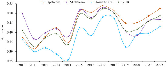
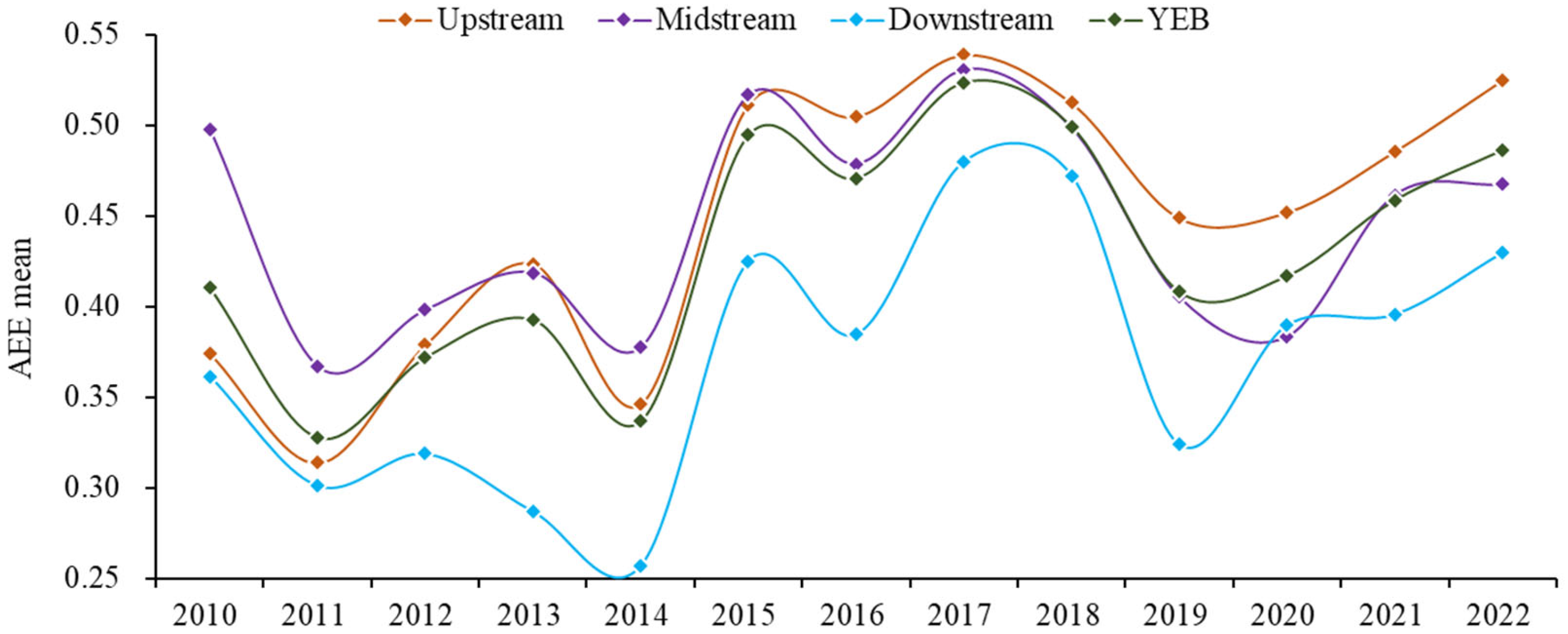
From 2010 to 2022, the AEE of the YEB exhibited a significant upward trend with fluctuations (Figure 2). The average value started at 0.410 in 2010. After experiencing periodic declines between 2011 and 2014, it surged significantly to 0.495 in 2015. Although some fluctuations occurred thereafter, the value reached a relatively high level of 0.486 by 2022, reflecting an overall positive trajectory. This evolution suggests that, as the YEB strategy proposed in 2014 has deepened, a series of environmental regulatory policies and agricultural green transition measures have begun to yield results, driving agricultural production toward resource conservation and environmental sustainability. However, the efficiency value remained below 0.5 for most of the study period (except in 2015 and 2017), with notable declines observed in certain years such as 2014 and 2019. This indicates that the overall AEE in the YEB remains at a moderate level. Its improvement process is nonlinear and susceptible to multiple factors such as climate change, policy implementation, and shifts in factor inputs, posing challenges to sustained enhancement.

Figure 2. Changes in the mean AEE of the YEB from 2010 to 2022. Note: The upstream region includes Chongqing, Sichuan, Guizhou, and Yunnan; the midstream region includes Hubei, Hunan, and Jiangxi; and the downstream region includes Shanghai, Jiangsu, Zhejiang, and Anhui.

Regionally, the evolution of AEE exhibits distinct patterns across the upstream, midstream, and downstream regions. The upstream region initially exhibited lower efficiency levels but showed a clear upward trend, rising steadily from 0.374 in 2010 to 0.525 in 2022. This improvement can likely be attributed to its relatively robust ecological foundation, combined with the synergistic effects of later-stage ecological conservation policies and specialized agricultural development initiatives. The AEE in the midstream region consistently fluctuated at a high level, with its average ranking among the highest. However, its stability remained relatively weak, particularly showing a noticeable decline in 2019–2020. This reflects that, while maintaining high agricultural output, the region faces substantial resource and environmental pressure as well as resistance to transformation. The average AEE in the downstream region remained relatively low with the greatest fluctuations, hitting a trough of 0.257 in 2014. This indicates that the squeezing effect of large-scale urbanization and industrialization on agricultural production, coupled with environmental constraints, was pronounced in this area. Nevertheless, a recovery trend emerged after 2015, likely to benefit from increased investments in technology-intensive agriculture and environmental governance.

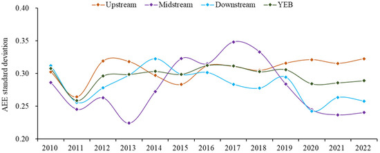
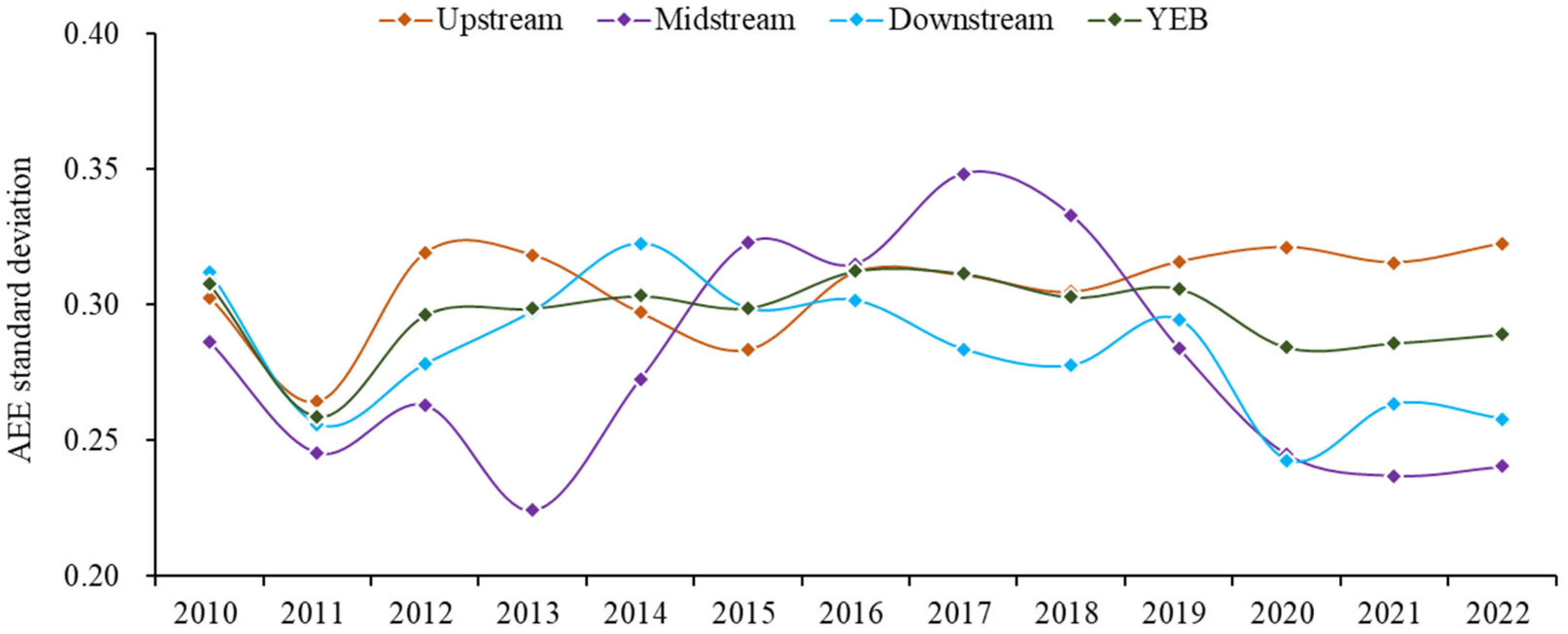
The standard deviation of AEE across the entire YEB declined slightly from 0.308 in 2010 to 0.289 in 2022, indicating a modest reduction in inter-county disparity. However, this trend was nonlinear, with notable increases in 2012–2014 and 2016–2017. Among subregions, the upstream region exhibited the highest and most persistent variability (ranging from 0.283 to 0.323), reflecting heterogeneous natural conditions and divergent development stages. The midstream region saw a clear downward trend (from 0.286 to 0.240), suggesting growing homogeneity in eco-efficiency within this traditional grain-producing area. The downstream region experienced the largest reduction (from 0.312 to 0.258), implying that urbanization and technological diffusion helped narrow the efficiency gap among its economically advanced counties (Figure 3).

Figure 3. Changes in AEE standard deviation in the YEB from 2010 to 2022.

3.2. Regional Inequality of AEE

Based on the Dagum Gini coefficient, the regional inequality in AEE across counties within the YEB from 2010 to 2022 exhibited fluctuating declines but remained significant (Table 2). The overall Gini coefficient ranged between 0.615 and 0.870, with a clear downward trend after 2015, reaching its lowest value of 0.615 in 2017. This suggests that regional coordination and green transition policies may have contributed to spatial equilibrium in AEE to some extent. However, the inequality rebounded in 2019–2020 (to 0.795 and 0.793, respectively), indicating vulnerability to external shocks such as extreme weather events or policy adjustments. In terms of the sources of inequality, the contribution of hyper-variance density (G_t) dominated in most years (exceeding 50% in 10 out of 13 years), implying that the primary driver of overall inequality is not simply intra- or inter-regional disparities, but rather the overlapping distribution of high- and low-efficiency counties across the three subregions. This spatial interlacing underscores the importance of cross-regional spillover effects and suggests that policies targeting administrative boundaries alone may be insufficient to reduce inequality.

Table 2. Regional inequality in AEE and its sources in the YEB from 2010 to 2022.

Year	Dagum Gini Coefficient				Contribution Rate (%)
	Total	Gw	Gb	Gt	Gw	Gb	Gt
2010	0.778	0.275	0.098	0.405	35.31%	12.66%	52.03%
2011	0.870	0.310	0.064	0.496	35.64%	7.30%	57.06%
2012	0.831	0.305	0.009	0.517	36.71%	1.02%	62.27%
2013	0.820	0.314	0.141	0.365	38.29%	17.17%	44.55%
2014	0.861	0.319	0.108	0.434	37.08%	12.50%	50.43%
2015	0.661	0.244	0.017	0.401	36.86%	2.52%	60.63%
2016	0.715	0.266	0.054	0.394	37.26%	7.54%	55.20%
2017	0.615	0.225	0.011	0.378	36.60%	1.85%	61.55%
2018	0.654	0.239	0.014	0.401	36.58%	2.15%	61.28%
2019	0.795	0.304	0.160	0.331	38.23%	20.16%	41.61%
2020	0.793	0.298	0.112	0.383	37.60%	14.08%	48.32%
2021	0.752	0.283	0.098	0.370	37.68%	13.06%	49.26%
2022	0.694	0.258	0.070	0.367	37.13%	10.02%	52.85%

In more detail, the contribution rate of intra-regional Gini (G_w) remained consistently stable between 35% and 38%, representing the most stable component among the three sources. This indicates that the imbalance in AEE among counties within the upstream, midstream, and downstream regions has persisted over the long term and exerts a significant impact. The contribution rate of inter-regional Gini (G_b) fluctuated dramatically, ranging from 1.02% to 20.16%, with particularly high peaks in 2013 and 2019. This reflects that disparities in AEE between the three major reaches were especially pronounced during certain periods. Notably, the contribution rate of G_t dominated in most years, exceeding 50% in 10 out of 13 years and peaking at 62.27%. This indicates that the primary source of regional inequality stems not from simple intra- or inter-regional disparities, but rather from the overlapping and intersecting distribution of AEE across counties in the upstream, midstream, and downstream regions. In other words, high-efficiency and low-efficiency counties are not spatially segregated strictly along watershed boundaries; instead, they exhibit an interwoven distribution pattern. This spatial complexity amplifies regional disparities and suggests that cross-regional factors, such as technology diffusion, factor mobility, or pollution spillover, exert profound effects on efficiency distribution.

3.3. Spatiotemporal Patterns of AEE

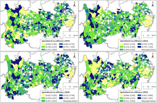
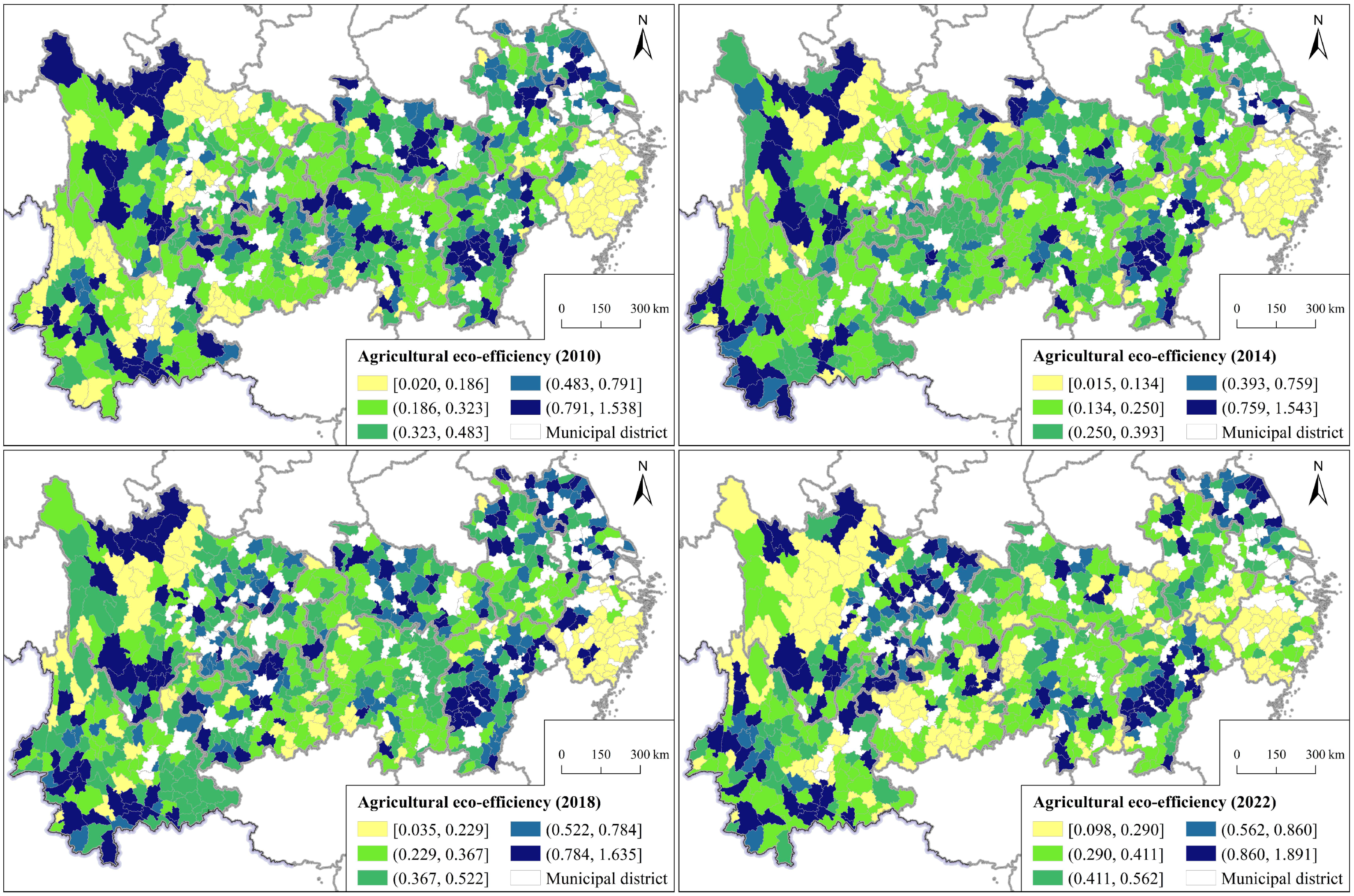
Spatially, the AEE in the YEB exhibited persistent spatial differentiation from 2010 to 2022 (Figure 4). In 2010, AEE showed significant spatial variation, yet overall efficiency levels remained low, with high-value counties scattered sporadically. By 2014, efficiency levels across all tiers had shifted downward, accompanied by a notable expansion in the scope of low-efficiency counties. This trend likely reflects a widespread intensification of resource and environmental pressures on regional agricultural production during this period. In 2018, AEE entered a recovery phase, characterized not only by significant upward shifts in the thresholds of all efficiency tiers but also by a gradual expansion in the coverage of higher-efficiency counties. In 2022, the efficiency range increased further, with the lowest threshold approaching the median level observed in 2010, indicating substantial improvements in AEE across most counties. Nevertheless, high-efficiency and low-efficiency counties continue to coexist spatially. Efficiency in some upstream mountainous areas and certain downstream regions remains lagging, indicating that the region’s spatial imbalance, marked by overall improvement yet persistent disparities, remains pronounced. Consequently, collaborative efficiency enhancement still faces structural challenges.

Figure 4. Spatial patterns of AEE in the YEB for the years of 2010, 2014, 2018, and 2022.

During the study period, the global Moran’s I index for AEE was significantly positive in each year, indicating that AEE consistently exhibited a significant positive spatial autocorrelation (Table 3). From an evolutionary perspective, the Moran’s I index fluctuated between 0.131 and 0.187, showing no sustained upward or downward trend. This indicates that while the intensity of spatial clustering is significant, it remains relatively stable over time. Overall, despite interannual fluctuations in agglomeration intensity, the spatial dependency pattern has remained stable. This further confirms that AEE is not randomly distributed across space; rather, persistent mutual influences and linkage effects exist between counties. These findings provide a basis for employing spatial econometric models to diagnose influencing factors.

Table 3. Global Moran’s I index of AEE in YEB from 2010 to 2022.

Year	Moran’s I	Year	Moran’s I	Year	Moran’s I
2010	0.158 ***	2015	0.186 ***	2020	0.135 ***
2011	0.179 ***	2016	0.147 ***	2021	0.165 ***
2012	0.146 ***	2017	0.157 ***	2022	0.158 ***
2013	0.187 ***	2018	0.132 ***
2014	0.131 ***	2019	0.138 ***

Note: *** p < 0.01.

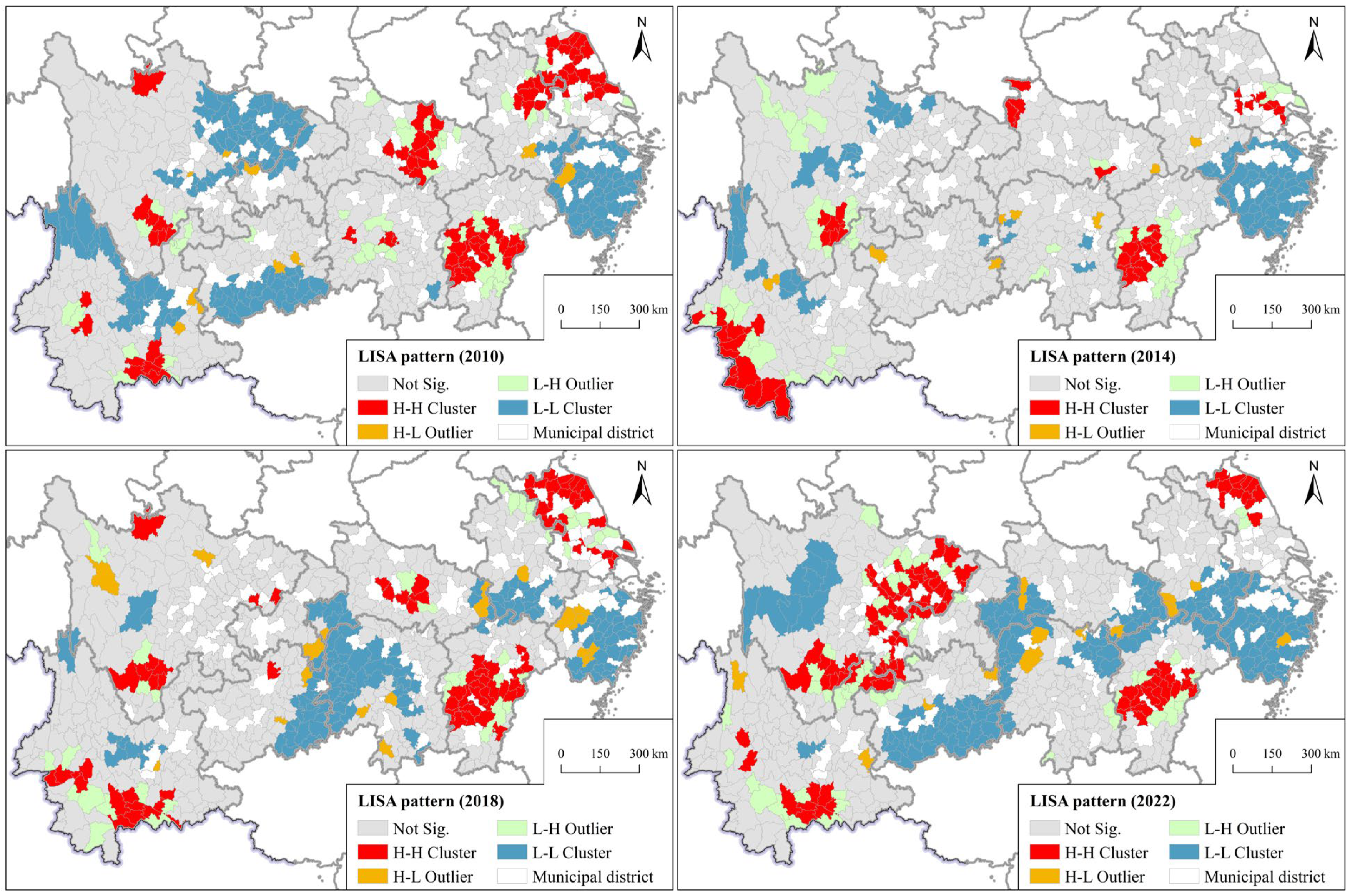
In terms of local spatial autocorrelation patterns, the AEE in the YEB exhibits significant local clustering characteristics and dynamic evolution (Figure 5). Specifically, in 2010, counties featured by high-high cluster were primarily distributed in northern Jiangsu, the Jianghan Plain, and central Jiangxi; those featured by low-low cluster were concentrated in Zhejiang, eastern Sichuan, southern Guizhou, and northern Yunnan. In 2014, as overall efficiency levels declined, the number of counties featured by both high-high and low-low clusters contracted significantly, with the former being mainly found in central Jiangxi and the western border regions of Yunnan and the latter being concentrated in Zhejiang. In 2018, the distribution of counties featured by high-high cluster remained similar to that in 2010, and those featured by low-low cluster were primarily concentrated in Zhejiang, southern Anhui, as well as the Wuling Mountain region and its surrounding areas. In 2022, counties exhibiting high-high cluster were primarily distributed in northern Jiangsu, central Jiangxi, eastern and southern Sichuan, and southern Yunnan; while those exhibiting low-low cluster expanded significantly, concentrated in Zhejiang, southern Anhui, the Hunan–Hubei–Jiangxi junction, western Hubei, western Hunan, southern Guizhou, and the western Sichuan plateau. Additionally, some counties exhibited low-high or high-low outliers across the four observation years, indicating localized spatial heterogeneity beyond the primary agglomeration patterns.

Figure 5. LISA patterns of AEE in the YEB for the years of 2010, 2014, 2018, and 2022.

3.4. Influencing Factors of AEE

3.4.1. Pre-Selection of Influencing Factors

AEE is shaped by the interplay of anthropogenic activities and natural environmental conditions. Human factors influence resource allocation, technological adoption, policy interventions, and economic restructuring, thereby altering the intensity of environmental emissions and the efficiency of resource use within agricultural systems. Natural factors, on the other hand, define the fundamental biophysical constraints and productive potential of agroecosystems, directly affecting primary productivity and ecological carrying capacity. Following established theoretical frameworks and empirical precedents [5,14,33,34], this study pre-selects nine variables spanning human and natural dimensions to systematically diagnose the determinants of AEE in the Yangtze River Economic Belt (YEB) (Table 4). The selection of each variable is grounded in its documented relevance to AEE dynamics, as elaborated below.

Table 4. Pre-selected influencing factors and their definitions.

Influencing Factors	Definitions
Economic development level (economic)	Per capita regional GDP based on the resident population (CNY/Person)
Urbanization rate (urban)	Urbanization rate based on permanent residents (%)
Rural residents’ income (income)	Per capita disposable income of rural households (CNY/Person)
Rural educational attainment (educate)	Average years of schooling for rural residents (Year)
Fiscal support for agriculture (fiscal)	Ratio of local public budget expenditures allocated to rural affairs (%)
Agricultural production structure (structure)	Share of grain crops in total sown area (%)
Temperature (temp)	Annual average temperature (℃)
Precipitation (prec)	Average daily precipitation (mm)
Net primary productivity (npp)	Net creation of organic matter by plant photosynthesis (-)

The human dimension comprises six factors. First, economic development level is proxied by per capita regional GDP. Higher economic development is generally associated with greater fiscal capacity for environmental governance, advanced infrastructure, and increased societal demand for ecological amenities, potentially exerting a positive influence on AEE through structural transformation and technological upgrading [14]. Second, the urbanization rate captures the degree of population concentration in urban areas. Urbanization may generate both positive effects, such as facilitating labor transfer from agriculture and relieving pressure on arable land, and negative externalities, including the encroachment of high-quality farmland and competition for water resources, which can influence AEE in complex ways [5,33]. Third, rural residents’ income, measured by per capita disposable income, reflects farmers’ economic incentives. Rising income can enable investments in productivity-enhancing and potentially environmentally intensive inputs unless accompanied by green production incentives, thereby exerting a theoretically ambiguous effect on AEE [34]. Fourth, rural educational attainment, measured as average years of schooling, represents human capital. While education is expected to improve farmers’ capacity to adopt sustainable practices, its actual effect on AEE may depend on the availability of green technologies and extension services; in their absence, better-educated farmers may prioritize labor-saving but input-intensive methods [34]. Fifth, fiscal support for agriculture, defined as the share of local public budget expenditures allocated to rural affairs, reflects policy priority. Such fiscal transfers are intended to improve agricultural infrastructure and promote technology diffusion, thereby positively contributing to AEE improvement [33]. Sixth, agricultural production structure, captured by the proportion of grain crops in total sown area, reflects land use specialization. A higher share of grain cultivation is often associated with more standardized and intensive production practices, which influence both resource efficiency and environmental pressure in distinct ways compared to more diversified or high-value cropping systems [14].

The natural dimension includes three variables. Temperature and precipitation are fundamental climatic factors governing crop growth duration, evapotranspiration rates, and nutrient cycling, directly shaping the efficiency of resource conversion in agricultural production. Net primary productivity serves as an integrated indicator of ecosystem vigor and biomass production capacity, reflecting the underlying ecological endowment that supports agricultural activities. Prior studies have demonstrated that spatial heterogeneity in AEE is closely tied to such biophysical gradients, particularly in topographically complex regions like the upper reaches of the YEB [14,33].

3.4.2. Diagnosis of Influencing Factors

To mitigate potential heteroscedasticity and enhance the interpretability of estimation results, logarithmic transformations were first applied to the three variables of economic development level (economic), rural residents’ income (income), and net primary productivity (npp). The collinearity diagnosis results indicate that the variance inflation factor (VIF) for all explanatory variables is below 5.0, with an average VIF of 2.183 (Table 5). This suggests that the model does not suffer from severe multicollinearity, and that the variable selection and model specification are reasonable.

Table 5. Collinearity diagnosis results.

Variable	VIF	1/VIF
lneconomic	4.081	0.245
urban	3.538	0.283
lnincome	2.969	0.337
educate	2.656	0.376
fiscal	1.108	0.903
structure	1.162	0.861
temp	1.552	0.644
prec	1.165	0.858
lnnpp	1.419	0.705
Mean VIF	2.183

Furthermore, the results of the spatial econometric model selection tests indicate that both the Wald and LR tests strongly reject the null hypothesis that the SDM can be degenerated into either the SLM or the SEM (all p-value = 0.001). Meanwhile, the Hausman test results significantly favor a fixed-effects model (Table 6). Based on a comprehensive analysis of the above test results, this study ultimately adopts a two-way fixed-effects SDM, which simultaneously captures the spatial spillover effects of both the dependent and independent variables, to more comprehensively and accurately diagnose the influencing factors of AEE in the YEB. After estimating the SDM, we conducted diagnostic tests on the residuals. The Moran’s I statistic for residual spatial autocorrelation was 0.023 (p = 0.312), indicating no significant remaining spatial dependence. The Breusch-Pagan test for heteroscedasticity yielded χ² = 15.67 (p = 0.074), suggesting no serious violation of homoscedasticity. These results confirm that the SDM specification adequately captures the spatial structure in the data.

Table 6. Selection test for spatial econometric model.

Items	Statistical Value	p-Value
Wald_spatial (Lag)	21.92	0.001
LR_spatial (Lag)	21.95	0.001
Wald_spatial (Error)	27.48	0.001
LR_spatial (Error)	27.84	0.001
Hausman Test	861.80	0.000

The estimation results of the SDM reveal the complex mechanisms influencing AEE in the YEB and their significant spatial spillover effects (Table 7). In terms of local direct effects, the coefficients for economic development level, urbanization rate, fiscal support for agriculture, and agricultural crop structure are significantly positive in both models. This indicates that the improvement in regional economic development level, factor agglomeration and industrial upgrading, government financial support for agriculture, and increase in the proportion of grain crops in total sown area brought about by local industrialization and urbanization processes all exert sustained positive effects on improving AEE. It is noteworthy that the coefficients of rural residents’ income and educational attainment are significantly negative. While this finding is statistically robust, its interpretation requires caution given the observational nature of the analysis and the absence of direct measures for green technology adoption or environmental regulation in the model. One plausible hypothesis is that, in the absence of complementary green technologies, extension services, effective regulations, higher income and education may inadvertently encourage the adoption of labor-saving but environmentally intensive practices to maximize output. However, alternative explanations cannot be ruled out. For instance, the negative association may reflect nonlinear relationships, omitted variable bias, or measurement mismatches between aggregate education/income data and actual farm-level production behaviors. Given these uncertainties, the observed negative coefficients should be interpreted as suggestive associations rather than definitive evidence of a “capability–behavior gap”. Future research incorporating granular data on green technology adoption and regulatory intensity is needed to disentangle these mechanisms. Among natural factors, temperature exhibits a positive influence, potentially benefiting the growth of various crops.

Table 7. Estimation results for the SDM.

	Inverse-Distance Weight Matrix		Economic Distance Weight Matrix
	Main	Wx	Main	Wx
lneconomic	0.017 *	0.110 ***	0.043 ***	0.062 ***
	(1.193)	(2.994)	(3.163)	(2.625)
urban	0.244 ***	−0.133 *	0.249 ***	−0.408 **
	(3.221)	(−0.480)	(3.273)	(−2.459)
lnincome	−0.038 **	0.023	−0.031 *	0.019
	(−2.111)	(0.579)	(−1.874)	(0.651)
educate	−0.046 ***	−0.044	−0.041 ***	−0.050
	(−3.227)	(−1.084)	(−3.002)	(−2.175)
fiscal	0.074 ***	−0.317	0.025 *	0.087
	(1.553)	(−2.167)	(0.548)	(0.943)
structure	0.061 ***	−0.023	0.055 **	0.004
	(2.594)	(−0.245)	(2.357)	(0.070)
temp	0.010 *	−0.012 *	0.026 **	−0.036 **
	(0.633)	(−0.484)	(2.057)	(−2.268)
prec	−0.002	0.011	0.020	−0.025
	(−0.274)	(0.770)	(3.120)	(−2.754)
lnnpp	−0.096	0.267 **	0.004	0.220 ***
	(−1.214)	(2.069)	(0.062)	(2.823)
rho	0.645 ***		0.194 ***
	(23.773)		(11.527)
County FE	Yes		Yes
Year FE	Yes		Yes
N	9477		9477
R2	0.012		0.008

Note: * p < 0.1, ** p < 0.05, *** p < 0.01; t-statistics in parentheses. County FE denotes county-level fixed effects, which control time-invariant unobserved heterogeneity across counties, and Year FE denotes year-fixed effects.

From the perspective of spatial spillover effects, the direction of influence exerted by factors differs markedly from that of local effects, revealing complex interregional interaction mechanisms. The per capita GDP of neighboring regions exhibits a significant positive spatial spillover effect, indicating that economic development in adjacent areas can generate positive externalities for the local region in terms of knowledge, technology, or environmental governance. NPP in neighboring areas also exhibits stable positive spillover effects, reflecting the spatial continuity of ecosystems and their positive impact on agricultural production. However, the coefficient for the urbanization rate of neighboring regions is significantly negative, suggesting that rapid urbanization in adjacent areas may exert pressure on local AEE through competition for and depletion of local labor and land resources, or through transboundary pollution. The negative spillover effects of temperature in adjacent regions may reflect shared risks or resource constraints faced by areas with homogeneous climatic conditions. Collectively, these findings confirm that neglecting spatial interaction effects will underestimate or misjudge the true impact of each factor.

Comparing the results under two spatial weight matrices, the direction and significance of the core influencing factors remained largely consistent, confirming the robustness of estimation results. Moreover, the strength of spatial autocorrelation under economic distance weight matrix is significantly lower than that under inverse distance weight matrix, indicating that spatial correlations in AEE are primarily driven by geographic proximity, while the role of economic similarity is relatively weaker. Taking together, these findings suggest that enhancing the AEE in the YEB requires not only optimizing local socioeconomic and natural conditions but also fully considering and effectively utilizing spatial interaction mechanisms across regions to formulate coordinated governance and differentiated strategies.

4. Discussion

This study develops a comprehensive evaluation index system to measure and spatially analyze AEE at the county level in the YEB from 2010 to 2022 and diagnoses the factors contributing to its regional disparities. The findings validate that AEE exhibits significant spatial dependence and reveal complex regional interaction mechanisms, offering new insights into the sustainable agricultural development in major river basins.

4.1. Further Theoretical Discussion

The AEE in YEB follows an evolutionary trajectory characterized by an overall upward trend interspersed with periodic fluctuations. A notable increase occurred after 2014, particularly between 2015 and 2017, coinciding with the implementation of the Yangtze River Economic Belt strategy [35]. While our empirical design is observational and does not establish causality, it is plausible that the strategy has exerted a systemic influence on regional agricultural production methods, through strengthened environmental regulations, promotion of green technologies, and industrial restructuring, thereby driving rapid efficiency improvements [36,37,38]. This interpretation is consistent with existing studies documenting positive environmental outcomes following major policy interventions in China [39]. However, the slowdown in efficiency gains after 2018 suggests that externally driven improvements may face diminishing returns, and continued progress will increasingly rely on endogenous drivers such as breakthroughs in green agricultural technologies, refinement of mechanisms for realizing the value of ecological products, and a substantial increase in the willingness and capacity of agricultural producers to transition toward green practices [5,40]. Similar patterns of policy-driven efficiency gains followed by stabilization have been observed in other contexts [41,42].

The spatial pattern of AEE is not only the result of static resource endowments and economic development but also reflects the dynamic interplay of spatial spillover effects. This study finds that hyper-variance intensity is the primary source of regional inequality, aligning with recent studies emphasizing the role of cross-regional interactions in shaping agricultural performance [43]. The SDM results further confirm that factors such as urbanization and economic development may exert opposite effects locally versus in neighboring areas, revealing a complex interplay of competition and cooperation. On the one hand, positive externalities such as knowledge accumulation and technological progress promote synergistic advancement through spatial spillover effects [44,45]. On the other hand, negative externalities such as competition for production factors like labor and water, as well as the transboundary transfer of pollution, may create spillover effects that shift burdens onto neighboring regions [46,47,48]. This coexistence of synergy and crowding explains why geographic proximity serves as a stronger spatial bond than economic similarity.

The spatial spillover effects of influencing factors challenge the adoption of uniform, one-size-fits-all policy approaches. The findings reveal a significant negative association between rural residents’ income and educational attainment and local AEE. While this result is statistically robust, its substantive interpretation must remain cautious, as the model does not include direct measures of green technology adoption, environmental regulation intensity, or farm-level behavioral responses. One speculative mechanism, drawing on the technology adoption literature [49], is that in the absence of supporting green technologies, market incentives, and effective regulation, increased income and knowledge may be directed toward expanding labor-saving yet environmentally costly production models, rather than invested in green innovation. This hypothesized “capability–behavior gap” is consistent with some studies showing that economic development without complementary environmental policies can exacerbate resource-intensive practices [5,40]. However, the current analysis cannot empirically verify this mechanism. Alternative explanations are equally plausible. For example, the negative association could arise from nonlinearities, omitted variable bias, or measurement error. Therefore, the “capability–behavior gap” should be viewed as one of several competing hypotheses warranting further investigation, rather than a conclusively demonstrated mechanism. What remains clear from the analysis is that simply raising farmers’ incomes or educational attainment may not automatically improve AEE, a finding that underscores the need for coordinated policy packages that couple human capital investment with accessible green technologies and enforceable environmental standards. Furthermore, fiscal support for agriculture exerts a significant positive effect locally, but its spatial spillover effects are insignificant. This suggests that current fiscal policies may be primarily focused on improving local agricultural production conditions and have yet to be effectively designed as a lever to promote interregional green technology cooperation and collaborative pollution control. These findings collectively underscore that enhancing agricultural eco-efficiency requires a sophisticated policy mix that balances local incentives with regional coordination, rather than advancing any single measure in isolation [5,50].

Additionally, while the spatial Durbin model with two-way fixed effects mitigates some concerns about omitted variable bias, the possibility of reverse causality cannot be entirely ruled out. Key explanatory variables such as economic development, rural household income, and urbanization may themselves be influenced by agricultural eco-efficiency, creating potential endogeneity. Therefore, the estimated coefficients should be interpreted as robust conditional associations rather than definitive causal effects. Future research employing instrumental variable strategies or lagged explanatory variables would help clarify causal direction.

4.2. Policy Implications

The empirical findings of this study, particularly regarding spatial clustering, regional inequality, and spillover effects, carry important implications for policy design.

First, spatially differentiated strategies should be tailored to regional efficiency patterns. The upstream regions have lower but rapidly improving AEE, benefiting from ecological advantages. Policies there should prioritize the development of specialized ecological agriculture, green product certification, and payment schemes for ecosystem services. The midstream regions exhibit high but volatile efficiency, indicating unsustainable intensification. These areas urgently need incentives for fertilizer/pesticide reduction, circular agriculture, and soil conservation. The downstream regions show low and unstable AEE due to urbanization pressures. They should leverage technological and financial resources to develop high-tech urban agriculture, smart agriculture, and pollution control infrastructure.

Second, cross-regional coordination mechanisms should be established to manage spatial spillovers. The findings that hyper-variance density dominates regional inequality, and that neighboring economic development exerts positive spillovers while neighboring urbanization exerts negative effects, call for collaborative governance. High-high cluster should serve as green technology diffusion hubs, with fiscal support for interregional knowledge transfer. Low-low clusters require joint ecological compensation programs and cross-boundary pollution control agreements. Through infrastructure connectivity, unified market rules, and coordinated environmental protection and governance, positive spillover effects can be promoted while negative ones are curbed.

Third, rural development policies should be redesigned to bridge the “capability–behavior gap”. The counterintuitive negative association between rural income/education and AEE suggests that economic and human capital gains alone do not automatically green agricultural practices. Governments should couple income support and educational investment with accessible green extension services, subsidized low-input technologies, and premium markets for eco-friendly products. Environmental regulations (e.g., caps on fertilizer use, penalties for pollution) must be strengthened to prevent income-induced intensification from undermining eco-efficiency. A coordinated package of measures, rather than isolated interventions, is required.

Fourth, fiscal support for agriculture should be optimized to stimulate interregional cooperation. While local fiscal spending on agriculture positively affects AEE, its spatial spillover effects are insignificant, indicating that current policies are too locally focused. A portion of agricultural funds should be reallocated to cross-regional green technology demonstration projects, joint research on pollution control, and ecological compensation transfers. Performance metrics for local governments should include not only their own AEE improvements but also contributions to raising efficiency in neighboring counties. Such reforms would turn fiscal policy into a lever for spatial synergy rather than isolated local gains.

4.3. Limitations and Future Prospects

This study has several limitations. First, regarding the measurement of AEE, the super-efficiency SBM model, while appropriate for handling undesirable outputs and slack variables, is sensitive to outliers and the choice of input/output indicators [51]. Although we kept the number of indicators within recommended limits relative to the number of DMUs, alternative specifications could yield different efficiency estimates. Second, county-level data in the YEB, particularly for agricultural nonpoint source pollution and carbon emissions, rely on estimation methods that introduce measurement error. The entropy method, while commonly used, involves subjective choices in normalization and weighting. Third, missing data were imputed using KNN and linear interpolation. Although summary statistics before and after imputation showed no significant differences, imputation may still affect precision. Fourth, the exclusion of municipal districts and two newly established counties, though necessary for data consistency, reduces representativeness, particularly for the downstream regions where urban agriculture plays an increasing role. Fifth, the analysis assumes linear and contemporaneous relationships between influencing factors and AEE, while nonlinear effects, spatial heterogeneity in coefficients, and temporal lags were not explored. Sixth, the observational design does not support causal inference. The associations identified, though robust to alternative spatial weight matrices, should not be interpreted as causal effects.

Future research could extend this work in several directions. First, longer time series and quasi-experimental methods, such as difference-in-differences (DID), should be employed to identify the causal impacts of specific policies such as ecological compensation or demonstration zones. Second, more refined measures of green technology adoption and farm-level environmental behavior need to be incorporated. Third, methods such as panel threshold models or geographically weighted regression could be employed to explore nonlinear and spatially varying relationships. Fourth, comparative studies across different major river basins are warranted to assess the generalizability of our findings. Fifth, greater attention should be paid to improving data quality and coverage, particularly for nonpoint source pollution and urban agriculture. Finally, due to data availability at the county level over the long study period, some theoretically important proximate determinants, such as environmental regulation intensity, green technology adoption, farm structure, and irrigation efficiency, had to be omitted. This limitation likely contributes to the relatively low explanatory power of the SDM and underscores the need for future research to incorporate finer-grained, survey- or remote sensing-based indicators to better capture the causal mechanisms underlying AEE.

5. Conclusions

This study constructed a comprehensive evaluation index system incorporating factor inputs, expected outputs, and undesirable outputs. Using the super-efficiency SBM model and spatial Durbin model, it analyzed the spatiotemporal patterns, regional inequality, and influencing factors of AEE at the county level in the YEB from 2010 to 2022.

The main empirical findings are threefold. First, the overall AEE of the YEB exhibited a fluctuating upward trend during the study period but remained below 0.5 in most years, indicating considerable room for improvement. Significant heterogeneity existed across the upstream, midstream, and downstream regions in terms of efficiency levels, stability, and evolutionary trajectories. Second, AEE exhibited significant positive spatial autocorrelation, with persistent high-high and low-low clusters. Regional inequality, as measured by the Dagum Gini coefficient, was primarily driven by hyper-variance intensity, suggesting that high- and low-efficiency counties are spatially interwoven rather than strictly separated by watershed boundaries. Third, the SDM results revealed that local economic development, urbanization, fiscal support for agriculture, and agricultural production structure had positive direct effects on AEE, whereas rural residents’ income and educational attainment showed negative associations. Spatial spillover effects were also significant: neighboring economic development and ecological conditions exerted positive externalities, while neighboring urbanization and temperature generated negative spillovers.

This study contributes to the literature by providing a county-level, long-term, spatially explicit assessment of AEE in the YEB that explicitly incorporates undesirable outputs and spatial spillover mechanisms. The findings deepen the understanding of the driving forces behind AEE and offer a scientific basis for formulating collaborative policies for the green transformation of agriculture in major river basins.

References

- Adenle, A.A.; Azadi, H.; Manning, L. The era of sustainable agricultural development in Africa: Understanding the benefits and constraints. Food Rev. Int. 2018, 34, 411–433. [Google Scholar]
- Streimikis, J.; Baležentis, T. Agricultural sustainability assessment framework integrating sustainable development goals and interlinked priorities of environmental, climate and agriculture policies. Sustain. Dev. 2020, 28, 1702–1712. [Google Scholar] [CrossRef] [Scilit]
- Jiao, X.Q.; He, G.; Cui, Z.L.; Shen, J.B.; Zhang, F.S. Agri-environment policy for grain production in China: Toward sustainable intensification. China Agric. Econ. Rev. 2018, 10, 78–92. [Google Scholar] [CrossRef] [Scilit]
- Shahmohamadloo, R.S.; Febria, C.M.; Fraser, E.D.; Sibley, P.K. Sustainable agriculture imperative: A perspective on the need for an agrosystem approach to meet the United Nations Sustainable Development Goals by 2030. Integr. Environ. Assess. Manag. 2021, 18, 1199–1205. [Google Scholar] [CrossRef] [Scilit] [PubMed]
- Wang, G.; Shi, R.; Mi, L.; Hu, J. Agricultural eco-efficiency: Challenges and progress. Sustainability 2022, 14, 1051. [Google Scholar] [CrossRef] [Scilit]
- Wang, N.; Li, S.; Kang, Q.; Wang, Y. Exploring the land ecological security and its spatio-temporal changes in the Yangtze River Economic Belt of China, 2000–2020. Ecol. Indic. 2023, 154, 110645. [Google Scholar] [CrossRef] [Scilit]
- Wei, M.; Chen, W.; Wang, Y. Assessment of the implementation effects of main functional area planning in the Yangtze River Economic Belt. Land 2024, 13, 940. [Google Scholar] [CrossRef] [Scilit]
- Jin, G.; Yu, H.; He, D.; Guo, B. Agricultural production efficiency and ecological transformation efficiency in the Yangtze River Economic Belt. Land 2024, 13, 103. [Google Scholar] [CrossRef] [Scilit]
- Xue, L.; Hou, P.; Zhang, Z.; Shen, M.; Liu, F.; Yang, L. Application of systematic strategy for agricultural non-point source pollution control in Yangtze River basin, China. Agric. Ecosyst. Environ. 2020, 304, 107148. [Google Scholar] [CrossRef] [Scilit]
- Coluccia, B.; Valente, D.; Fusco, G.; De Leo, F.; Porrini, D. Assessing agricultural eco-efficiency in Italian regions. Ecol. Indic. 2020, 116, 106483. [Google Scholar] [CrossRef] [Scilit]
- Pishgar-Komleh, S.H.; Čechura, L.; Kuzmenko, E. Investigating the dynamic eco-efficiency in agriculture sector of the European Union countries. Environ. Sci. Pollut. Res. 2021, 28, 48942–48954. [Google Scholar] [CrossRef] [Scilit]
- Wang, G.; Zhao, M.; Zhao, B.; Liu, X.; Wang, Y. Reshaping agriculture eco-efficiency in China: From greenhouse gas perspective. Ecol. Indic. 2025, 172, 113268. [Google Scholar] [CrossRef] [Scilit]
- Xu, T.; Gao, P.; Yu, Q.; Fang, D. An improved eco-efficiency analysis framework based on slacks-based measure method. Sustainability 2017, 9, 952. [Google Scholar]
- Liu, Y.; Zou, L.; Wang, Y. Spatial-temporal characteristics and influencing factors of agricultural eco-efficiency in China in recent 40 years. Land Use Policy 2020, 97, 104794. [Google Scholar] [CrossRef] [Scilit]
- Li, S.; Zhu, Z.; Dai, Z.; Duan, J.; Wang, D.; Feng, Y. Temporal and spatial differentiation and driving factors of China’s agricultural eco-efficiency considering agricultural carbon sinks. Agriculture 2022, 12, 1726. [Google Scholar] [CrossRef] [Scilit]
- Liao, J.; Yu, C.; Feng, Z.; Zhao, H.; Wu, K.; Ma, X. Spatial differentiation characteristics and driving factors of agricultural eco-efficiency in Chinese provinces from the perspective of ecosystem services. J. Clean. Prod. 2021, 288, 125466. [Google Scholar] [CrossRef] [Scilit]
- Li, Y.; Yang, Q.; Cao, Z. Current characteristics and model transformation of agricultural development in the Yangtze River Economic Belt. Prog. Geogr. 2015, 34, 1458–1469. [Google Scholar]
- Wang, Y.; Zhang, A. Spatiotemporal evolution and trend of cultivated land pressure in the Yangtze River Economic Belt. Resour. Environ. Yangtze Basin 2022, 31, 461–471. [Google Scholar]
- Liu, Z.; Yang, D.; Wen, T. Agricultural production mode transformation and production efficiency: A labor division and cooperation lens. China Agric. Econ. Rev. 2019, 11, 160–179. [Google Scholar] [CrossRef] [Scilit]
- Luo, J.; Jin, X.; Liu, J.; Liang, X.; Han, B.; Zhou, Y. Changes and influencing factors of agricultural eco-efficiency in northern Jiangsu from 2000 to 2020. Trans. Chin. Soc. Agric. Eng. 2023, 39, 239–248. [Google Scholar]
- Maia, R.; Silva, C.; Costa, E. Eco-efficiency assessment in the agricultural sector: The Monte Novo irrigation perimeter, Portugal. J. Clean. Prod. 2016, 138, 217–228. [Google Scholar] [CrossRef] [Scilit]
- Li, B.; Zhang, J.; Li, H. Spatiotemporal characteristics and influencing factor decomposition of agricultural carbon emissions in China. China Popul. Resour. Environ. 2011, 21, 80–86. [Google Scholar]
- Sun, Y.; Su, X.; Xu, G. Correlation between intensive cultivated land use level and carbon emission efficiency in Hebei province. Trans. Chin. Soc. Agric. Eng. 2016, 32, 258–267. [Google Scholar]
- Ding, X.; Wu, Q.; Wen, G.; Zhang, C. Migration trajectory and spatial pattern of cultivated land non-point source pollution in the Dongting Lake Plain from 2005 to 2019. Trans. Chin. Soc. Agric. Eng. 2021, 37, 258–266. [Google Scholar]
- Zhu, Y.; Tian, D.; Yan, F. Effectiveness of entropy weight method in decision-making. Math. Probl. Eng. 2020, 2020, 3564835. [Google Scholar] [CrossRef] [Scilit]
- Cook, W.D.; Seiford, L.M. Data envelopment analysis (DEA)–Thirty years on. Eur. J. Oper. Res. 2009, 192, 1–17. [Google Scholar]
- Tone, K. A slacks-based measure of efficiency in data envelopment analysis. Eur. J. Oper. Res. 2001, 130, 498–509. [Google Scholar] [CrossRef] [Scilit]
- Anselin, L. The Moran scatterplot as an ESDA tool to assess local instability in spatial association. In Spatial Analytical Perspectives on GIS; Routledge: London, UK, 2019; pp. 111–126. [Google Scholar]
- LeSage, J.; Pace, R.K. Introduction to Spatial Econometrics; Chapman and Hall/CRC: Boca Raton, FL, USA, 2009. [Google Scholar]
- Elhorst, J.P. Spatial Econometrics: From Cross-Sectional Data to Spatial Panels; Springer: Berlin/Heidelberg, Germany, 2013. [Google Scholar]
- Getis, A.; Aldstadt, J. Constructing the spatial weights matrix using a local statistic. Geogr. Anal. 2004, 36, 90–104. [Google Scholar] [CrossRef]
- Yang, J.; Huang, X. 30 m annual land cover and its dynamics in China from 1990 to 2019. Earth Syst. Sci. Data 2021, 13, 3907–3925. [Google Scholar] [CrossRef] [Scilit]
- Wu, Y.; Rahman, R.A.; Yu, Q. Analysis of the spatial characteristics and influencing factors of agricultural eco-efficiency: Evidence from Anhui Province, China, during the period 2011–2018. Environ. Monit. Assess. 2022, 194, 154. [Google Scholar] [CrossRef] [Scilit] [PubMed]
- Zhang, Z.; Jin, G. Measurement of agricultural eco-efficiency and analysis of its influencing factors: Insights from 44 agricultural counties in Liaoning province. Land 2024, 13, 300. [Google Scholar] [CrossRef] [Scilit]
- Zhang, Z.; Zhang, L.; Liang, T.; Cheng, L.; Fang, L.; Zhao, B.; Zhang, J.; Wen, C. Has the Yangtze River Economic Belt strategy promoted the construction of ecological civilization in the upper reaches of the Yangtze River? Front. Environ. Sci. 2022, 10, 1046323. [Google Scholar]
- Li, E.; Ren, S.; Yang, Y. Green transformation mechanisms and implementation path for agricultural clusters: A case study of the vegetable cluster in Shouguang city, Shandong province, China. J. Geogr. Sci. 2024, 34, 2393–2420. [Google Scholar] [CrossRef] [Scilit]
- Wang, X.Q.; Lin, C.S. Green development research in China: A bibliometric analysis and systematic review. Appl. Ecol. Environ. Res. 2025, 23, 11359–11386. [Google Scholar] [CrossRef] [Scilit]
- Xu, M. Can the ecological protection red line policy promote food security? Based on the empirical analysis of land protection in China. Front. Environ. Sci. 2025, 13, 1654217. [Google Scholar] [CrossRef] [Scilit]
- Yan, B.; Wu, L.; Wang, X.; Wu, J. How can environmental intervention work during rapid urbanization? Examining the moderating effect of environmental performance-based accountability in China. Environ. Impact Assess. Rev. 2021, 86, 106476. [Google Scholar] [CrossRef] [Scilit]
- Grzelak, A.; Guth, M.; Matuszczak, A.; Czyżewski, B.; Brelik, A. Approaching the environmental sustainable value in agriculture: How factor endowments foster the eco-efficiency. J. Clean. Prod. 2019, 241, 118304. [Google Scholar] [CrossRef] [Scilit]
- Chen, S.; Li, G. How can grain price support policies enhance stable and increased wheat production? A risk aversion and cost saving perspective. Front. Sustain. Food Syst. 2025, 9, 1570962. [Google Scholar] [CrossRef] [Scilit]
- Jewell, J.; Cherp, A.; Geels, F.W.; Suzuki, M.; Nacke, L.; Tosun, J.; Bhowmik, S.; Kalzlou, T.; Jakhmola, A.; Vinichenko, V. Policy-driven growth of technologies to accelerate climate action. Nat. Rev. Earth Environ. 2026, 7, 235–252. [Google Scholar] [CrossRef] [Scilit]
- Lin, L.; Huang, F.; Li, X.; Zheng, J.; Wang, M. How Trade Competitiveness Drives High-Quality Agricultural Development: The Roles of Agricultural Structural Transformation and Regional Innovation. Sustainability 2026, 18, 1676. [Google Scholar] [CrossRef] [Scilit]
- Audretsch, D.B.; Feldman, M.P. Knowledge spillovers and the geography of innovation. In Handbook of Regional and Urban Economics; Elsevier: Amsterdam, The Netherlands, 2004; Volume 4, pp. 2713–2739. [Google Scholar]
- You, J.; Tang, C.; Han, X.; Li, L. Technology transfer, knowledge spillover and industrial green transformation from the perspective of externalities. Reg. Stud. 2025, 59, 253–258. [Google Scholar] [CrossRef] [Scilit]
- Chunsuttiwat, P. Three Essays on the Transboundary Spillover of Negative Environmental Externalities, Social Inequality, and Public Policy. Ph.D. Thesis, The University of Wisconsin-Madison, Madison, WI, USA, 2022. [Google Scholar]
- Hosoe, M.; Naito, T. Trans-boundary pollution transmission and regional agglomeration effects. Pap. Reg. Sci. 2006, 85, 99–119. [Google Scholar]
- Zhao, Y.; Liang, C.; Zhang, X. Positive or negative externalities? Exploring the spatial spillover and industrial agglomeration threshold effects of environmental regulation on haze pollution in China. Environ. Dev. Sustain. 2021, 23, 11335–11356. [Google Scholar]
- Gallardo, R.K.; Sauer, J. Adoption of labor-saving technologies in agriculture. Annu. Rev. Resour. Econ. 2018, 10, 185–206. [Google Scholar] [CrossRef] [Scilit]
- He, X.; Liu, W. Coupling coordination analysis between farmland transfer and agricultural eco-efficiency in China. Agriculture 2024, 14, 2172. [Google Scholar] [CrossRef] [Scilit]
- Xu, K.; Bossink, B.; Chen, Q. Efficiency evaluation of regional sustainable innovation in China: A slack-based measure (SBM) model with undesirable outputs. Sustainability 2019, 12, 31. [Google Scholar] [CrossRef] [Scilit]
Disclaimer/Publisher’s Note: The statements, opinions and data contained in all publications are solely those of the individual author(s) and contributor(s) and not of MDPI and/or the editor(s). MDPI and/or the editor(s) disclaim responsibility for any injury to people or property resulting from any ideas, methods, instructions or products referred to in the content. |
© 2026 by the authors. Licensee MDPI, Basel, Switzerland. This article is an open access article distributed under the terms and conditions of the Creative Commons Attribution (CC BY) license.