Optimization Model of Transit Route Fleet Size Considering Multi Vehicle Type

Abstract

This paper proposes a bus line capacity optimization design model considering the scale of multiple vehicles, which is achieved by minimizing system operating costs and user costs. The proposed model takes into account the difference of passenger demand in different periods, and can get the optimal headway and delivery and reserve plan. In order to prove that the method can effectively minimize the cost, we solved a numerical example and compared the cost of the method in multi-transit model planning. Furthermore, the optimization results show that the total costs (TC) were reduced by 14.48%. Among them, the user costs (UC) decreased by 30.38% and the operator costs (OC) increased by 4.18%. Sensitivity analyses are presented to verify the validity of the model. The analysis results show that multi size bus optimization can reduce the total cost, especially the user cost in a certain cost weight interval. Besides this, the cost weight which reflects the passenger volume and waiting time value, optional bus size and cross-section passenger volume all affect vehicle scheme and system cost.

1. Introduction

The vehicle is an important carrier to provide public transport services. The rational allocation of line capacity structure is the key to optimize the allocation of resources in public transport operation and management. Two problems should be considered in bus line capacity allocation, bus size and quantity, which have an important impact on the efficient operation of public transport and the quality and level of service perceived by the user. In the past, in-depth research on the optimum size and type of buses took place and a whole series of policies were developed which gave priority to public transport to try and deal with traffic congestion in large urban areas.

Walters [1] arrived at a conclusion for bus size in the situation of competition and points out the benefits of using small buses on public transport networks. Glaister [2] noted that small vehicles will often have a competitive advantage over the traditional size. On dense routes, they may operate in competition with larger vehicles offering a faster service at a premium price. There might be significant adverse effects on traffic congestion. Oldfield and y Bly [3] gave a mathematical model which can be solved analytically to provide an explicit relationship between optimal bus size and factors such as operating cost, level of demand, and demand elasticities. Lee et al. [4] determined the vehicle size for bus operations by using classical analysis optimization to minimize the total cost of operators and users, and by applying multi-dimensional optimization algorithms to minimize system costs. Fu and Ishkhanov [5] developed a heuristic procedure to determine the best fleet combination of paratransit agencies, and used real examples to show the relationship between the performance of paratransit system and vehicle size. Hybrid fleets can reduce the total cost of the system when the demand density varies greatly over time or space. Jara-Díaz and Gschwender [6] developed an optimization model for fleet sizes considering budgetary constraints. Dell’Olio et al. [7] proposed a bi-level optimization planning model with bus capacity restrictions to determine the size and frequency of buses on each line. Kim and Schonfeld [8] proposed an optimization model for variable bus service and analyzed the impact of changes in demand on the effectiveness of variable bus services. They applied a simple heuristic method to the solution, which is not suitable for large problems involving multiple areas and multiple vehicle types. Ceder et al. [9] proposed a multi-objective method to determine vehicle dimensions and schedule buses by minimizing the determined headway and the expected headway deviation as the first objective, and by taking the observed load and the expected load deviation as the second objective. Ibeas et al. [10] proposed an optimization model for designing the intervals (headways) and sizes of buses circulating on public transport networks by minimizing the system’s operating and user costs. The validity of the proposed model is shown by applying it to the city of Santander, Spain. Ibarra-Rojas et al. [11] summarized issues related to bus network planning and real-time control strategies applicable to the bus system. Vazquez-Abad and Fenn, L. [12] developed the required theory to implement a mixed optimization procedure to find the optimal fleet size under a stationary probability constraint. Sergio Jara-Díaz et al. [13] considered the peak and off-peak hours of public transportation to find the optimal fleet size, frequency and vehicle capacity. Li et al. [14] proposed an approach called new life additional benefit-cost to solve the mixed bus fleet management problem for maximizing the total net benefit of early replacement, where both the optimal fleet size and composition under budget constraints can be determined. Liang et al. [15] discussed the relationship between the standard deviation of bus departure intervals and the number of buses, and proposed a model to explore the number of buses on the route. AlKheder, S et al. [16] considered five different types of buses based on vehicle capacity and developed a model using integer planning with the goal of minimizing the total cost of the route, and applied it to the KPTC network with 35 lines and 457 buses. Liang et al. [17] presented a set of optimal control formulations to minimize the costs for the passengers and the bus company, taking into account the randomness of passenger arrivals and tested the effect of the optimization method. Tian et al. [18] proposed a modeling framework to determine the optimal bus fleet size and its assignment onto multiple bus lines in a bus service network considering uncertain demand and used mixed integer stochastic programming to formulate the problem. Jara-Díaz Sergio et al. [19] considered the differences in traffic conditions between peak and off-peak hours and raised a relevant strategic design choice regarding the potential use of vehicles with different sizes. Sun et al. [20] studied the development of a mixed integer non-linear model for optimizing multi-terminal CB service in an urban setting. A mixed bus fleet with various bus sizes was employed to accommodate passenger demand, which increases vehicle utilization and reduces supplier’s cost. Jiang et al. [21] proposed a mixed scheduling model for limited-stop buses and normal buses. This model can optimize the total cost in terms of waiting time, in-vehicle time and operation cost by simultaneously adjusting the frequencies of limited-stop buses and normal buses.

Existing research mostly solves the problem of a single-vehicle configuration. The same route or fleet considers fewer vehicle types and does not consider the difference in departure intervals of each vehicle type. Therefore, the contribution of this paper is to consider the difference in the departure intervals of each vehicle type to determine the optimal size of the multi-vehicle fleet, thereby reducing the total cost of bus system operation and users, at the same time improving the flexibility of public transportation supply.

In this paper, we propose a vehicle capacity optimization models which minimizes the cost both operator and user. The method allows differently sized buses to be assigned to one public transport line, and it is tested on real traditional transit line. The obtained results have shown that proposed method can reasonably configure the number and type of buses according to the passenger flow in different periods, and effectively reduce the cost of public transport system. The paper is organized as follows. Section 2 gives a formal description of the problem and puts forward all the assumptions and constraints used. Section 3 proposes the optimization model. Section 4 implements the optimization model to real traditional transit system. Lastly, Section 5 sums the results discusses areas of future research.

2. Problem Statement

In this section, the bus line capacity allocation problem in the bus system is explained. For simplicity, we make the following assumptions:

(i)

It does not consider the situation of two-way departure, so as to ensure the circulation of public transport vehicles;

(ii)

According to the passenger flow data, the bus operation time is divided into several periods, and the departure intervals are equal in the same period;

(iii)

Bus vehicles run in normal order, and there is no overtaking or jumping phenomenon. Headway of the vehicle arriving at the station is equal to departure intervals each period.

(iv)

Passengers arriving at the bus station are evenly distributed, and the public transit passenger flow is relatively stable at each time period. There is no passenger loss and all passengers can get on the car at one time;

(v)

Bus speed is only related to road traffic conditions, and it does not consider the impact of traffic accidents or road construction, and the speed of the bus is equal in the same period of time.

According to assumption (i), the idealized model treats the bus route as a dynamical system with operating buses moving at a constant average velocity around a circular route of length, with a single depot. According to assumptions (ii) and (iii), at any point in period j, headway of bus size i is evenly distributed on this circuit as $h_{ji}$. Besides this, all vehicles belonging to one bus company start another service trip from and end at the same terminal.

Bus transport capacity should match the demand of passenger flow, and it is necessary to avoid both inadequate and waste of transport capacity. Bus capacity demand normally varies significantly by different time period like peak and non-peak hours. According to assumption (ii), the running time should be measured for individual time period. Classify the period considering the operating characteristics and passenger demand and the capacity allocation scheme is matched for the same period defined as j. The method of reference [16] can be used for period division.

Considering the longer service life of vehicles, the purchase of vehicles does not belong to the regular behavior, and based on the assumption (iv), the state of the transport reserve capacity of the bus is in a relatively stable state during a certain period. The vehicle allocation scheme of period j is based on passenger demand and operation characteristics during this period, and is restricted by existing reserve capacity. Therefore, this paper has to solve two problems: (1) vehicle reserve capacity and structure, and (2) vehicle allocation plan in different periods. Define $N^{\ast }$ as the reserve capacity set, and $n_i^{\ast }$ is the reserve quantity of bus size i in the set. The reserve capacity $n_i^{\ast }$ and the allocation capacity of bus size i in j period which is defined as $n_{ji}$ conform to the following relation:

$$n_i^{\ast }\ge n_{ji}\left(n_i^{\ast }\in N^{\ast },\forall j,j\le J\right)$$

(1)

where J is the number of periods. To meet the passenger demand, $N_j$ is defined as the total number of vehicles allocated in the j period which should satisfy the following equation:

$$N_j={\displaystyle \sum _{i=1}^I{n}_{ji}}$$

(2)

where I is the number of bus size type. In order to meet the needs of vehicle cycle operation, based on the assumption (v), $h_{ji}$ should satisfy the following equalities:

$${\beta }_{ij}=\{\begin{array}{l}{\displaystyle \sum _{i=1}^I{n}_{ji}{h}_{ji}}=\frac{2L_{\gamma }}{v_j/60}\\ {\displaystyle \sum _{i=1}^I{m}_{ji}{h}_{ji}}=t{p}_j\\ {\displaystyle \sum _{i=1}^I{m}_{ji,peak}{h}_{ji}}=60\end{array}$$

(3)

where $L_{\gamma }$ is the length of route r (km), v_j is the average speed of bus in period j (km/h), $m_{ji,}$ represents departure number of bus size i in the period j (buses), $t{p}_j$ is the length of period j (min), $m_{ji,peak}$ represents departure number of bus size i in the peak-hour of period j (buses). The headway of the bus should meet the following conditions: $h_{\min }\le h_{ji}\le h_{\max }$, where $h_{\max }$ is the maximum headway (min) and $h_{\min }$ is the minimum headway (min).

$$h_{ji}·Q_{j,peak}/60\le q_i·{\eta }_{ji}$$

(4)

$m_{ji,peak}$, $m_{ji}$ can be expressed as:

$$\{\begin{array}{l}{m}_{ji,peak}=M_{j,peak}·n_{ji}/N_j\\ m_{ji}=M_j·n_{ji}/N_j\end{array}$$

(5)

$M_{j,peak}$, $M_j$ can be expressed as:

$$\{\begin{array}{l}{M}_{j,peak}=M_j·60/t{p}_j\\ M_j=N_j·t{p}_j·v_j/(120L_r)\end{array}$$

(6)

where $M_{j,peak}$ is the departure number of all bus size in the peak-hour of period j (buses). $M_j$ is the departure number of all bus size in the period j (buses).

Similarly, get down:

$$\{\begin{array}{l}{m}_{ji,peak}=m_{ji}·60/t{p}_j\\ m_{ji}=n_{ji}·t{p}_j·v_j/(120L_r)\end{array}$$

(7)

Length of departure time interval of bus size i within period j can be expressed as:

$$t{p}_{ji}=t{p}_j·\frac{m_{ji}{q}_i}{{\displaystyle \sum _{i=1}^I{m}_{ji}{q}_i}}$$

(8)

Then $h_{ji}$ can be expressed as:

$$h_{ji}=t{p}_{ji}/m_{ji}$$

(9)

Meanwhile, the maximum passenger flow that can be transported by public transport capacity $N_j$ should be matched with $Q_{j,peak}$ which is the peak-hour cross-section passenger volume in period j (PCPV) (pax/h). The formula is as follows:

$$Q_{j,peak}\le {\displaystyle \sum _{i=1}^I{q}_i{\eta }_j{m}_{ji,peak}}$$

(10)

It can be expressed as:

$$Q_{j,peak}\le \frac{{\eta }_j{v}_j{\displaystyle \sum _{i=1}^I{q}_i{n}_{ji}}}{2L_r}$$

(11)

where $q_i$ is the capacity of bus size i (pax/bus), ${\eta }_j$ is the fulfill load proportion in period j and it meets the following conditions: ${\eta }_{\min }\le {\eta }_j\le {\eta }_{\max }$, where ${\eta }_{\max }$ is the maximum fulfill load proportion and ${\eta }_{\min }$ is the minimum fulfill load proportion.

3. Proposed Model

3.1. Definition of Variables

The following symbols are used in this paper:

• $cp$ = hourly cost of personnel (¥/h);
• $c{f}_i$ = unit fixed cost per h of bus size i (¥/h/bus);
• $c{k}_i$ = unit cost per km covered by bus size i (¥/km);
• $h_{ji}$ = headway of bus size i within period j (min);
• $h_{\max }$ = maximum headway (min);
• $h_{\min }$ = minimum headway (min);
• i = bus size type;
• I = number of bus size considered;
• j = period type;
• J = number of period considered;
• $q_i$ = capacity of bus size i (pax/bus);
• $m_{ji}$ = departure number of bus size i in period j (buses);
• $M_j$ = total departure number of buses in period j (buses);
• $Q_j$ = passenger volume in period j (pax);
• $Q_{ji}$ = passenger flow borne by bus size i in period j (pax);
• $Q_{j,peak}$ = cross-section passenger volume in period j (PCPV) (pax/h);
• $n_{ji}$ = number of bus size i in period j (buses);
• $n_i^{\ast }$ = number of bus size i provided (buses);
• $N_j$ = total number of buses in period j (buses);
• $L_r$ = length of route r (km);
• $OC$ = operator costs of route r (¥);
• $r$ = public transport route;
• $t{p}_j$ = time length of period j (min);
• $t{p}_{ji}$ = length of departure time interval of bus size i within period j (min);
• $TC$ = total costs of route r (¥);
• $UC$ = user costs of route r (¥);
• $v_j$ = average speed of bus in period j (km/h);
• $\alpha$ = weight coefficient of user costs;
• $\beta$ = weight coefficient of operator costs;
• ${\eta }_j$ = the fulfill load proportion in period j;
• $\phi$ = value of waiting time (¥/h).

3.2. Mathematical Model

The optimization model of transit route capacity allocation is proposed based on minimizing the cost function for the users of the bus route and the running of the public transport service. This model objective function is total cost (TC), which takes into account the costs of public transport users (UC) and the operating costs of the public transport operating company (OC).

The user costs consist of access/egress times to and from bus stops, as well as waiting time, including in vehicle times and transfer times. Some costs such as access/egress times to and from bus stops, in vehicle and transfer times can be regarded as constant for a fixed route system. Based on the hypothesis (iv), the waiting time is a function of passenger volume and headway which are calculated as:

$$TWT={\displaystyle \sum _{j=1}^J{\displaystyle \sum _{i=1}^I{h}_{ji}{Q}_{ji}/(2·60)}}$$

(12)

where $Q_{ji}$ is the passenger flow borne by bus size i in period j, it can be calculated as:

$$Q_{ji}=Q_j·\frac{m_{ji}{q}_i}{{\displaystyle \sum _{i=1}^I{m}_{ji}{q}_i}}$$

(13)

According to the Formulas (7)–(9), $h_{ji}$ can be expressed as:

$$h_{ji}=\frac{120L_r{q}_i}{v_j{\displaystyle \sum _{i=1}^I{n}_{ji}{q}_i}}$$

(14)

According to Equations (6), (11)–(13), the user cost of waiting time is equal to:

$$UC={\displaystyle \sum _{j=1}^J{\displaystyle \sum _{i=1}^I\frac{\phi n_{ji}{Q}_j{L}_r{q}_i{}^2}{v_j{({\displaystyle \sum _{i=1}^I{n}_{ji}{q}_i})}^2}}}$$

(15)

The operating costs (OC) are the sum of direct costs plus indirect costs. The direct cost includes three factors: rolling cost (km coverage) (CK), personnel cost (CP) and fixed cost (CF). In previous research, it was found that indirect cost (CI) is about 12% of direct cost [22]. Then the operating costs can be calculated as:

$$OC=1.12(CK+CP+CF)$$

(16)

The total cost of the kilometers covered is equal to:

$$CK={\displaystyle \sum _{j=1}^J{\displaystyle \sum _{i=1}^{I}2L_r{m}_{ji}c{k}_i}}$$

(17)

According to Equations (6) and (16), the total cost of the kilometers covered can be written as:

$$CK={\displaystyle \sum _{j=1}^J{\displaystyle \sum _{i=1}^I{n}_{ji}t{p}_j{v}_{j}c{k}_i/60}}$$

(18)

Personnel costs are calculated as:

$$CP={\displaystyle \sum _{j=1}^{J}t{p}_j{N}_{j}cp/60}$$

(19)

According to Equation (2), personnel costs can be written as:

$$CP={\displaystyle \sum _{j=1}^J{\displaystyle \sum _{i=1}^{I}t{p}_j{n}_{ji}cp/60}}$$

(20)

Based on the number of buses required to provide the service, the fixed costs are calculated using the following formula, which can be expressed as:

$$CF={\displaystyle \sum _{j=1}^J{\displaystyle \sum _{i=1}^I{n}_i^{\ast }c{f}_i}t{p}_j/60}$$

(21)

The term fixed costs as used here is a cost function, which only applies to the bus size and the number of buses. It covers the costs of financing, insurance, and annual taxes generated by a vehicle of a certain size of buses. To be included in the objective function, a theoretical unit cost is calculated by dividing these annual costs of these vehicles by their annual service hours.

Based on this description, the optimization problem can be formulated as follows:

$$\min TC=\alpha UC+\beta OC$$

(22)

$$\begin{array}{ll}\min TC=& {\displaystyle \sum _{j=1}^J{\displaystyle \sum _{i=1}^I\frac{\alpha \phi n_{ji}{Q}_j{L}_r{q}_i{}^2}{v_j{({\displaystyle \sum _{i=1}^I{n}_{ji}{q}_i})}^2}}}+1.12\beta ({\displaystyle \sum _{j=1}^J{\displaystyle \sum _{i=1}^I{n}_{ji}t{p}_j{v}_{j}c{k}_i/60}}+\\ & {\displaystyle \sum _{j=1}^J{\displaystyle \sum _{i=1}^{I}t{p}_j{n}_{ji}cp/60}}+{\displaystyle \sum _{j=1}^J{\displaystyle \sum _{i=1}^I{n}_i^{\ast }c{f}_i}t{p}_j/60})\end{array}$$

(23)

Subject to:

$$\begin{array}{l}{Q}_{j,peak}\le {\eta }_j{v}_j{\displaystyle \sum _{i=1}^I{q}_i{n}_{ji}}/2L_r\\ n_i^{\ast }\ge n_{ji}\\ h_{\min }\le \frac{120L_r{q}_i}{v_j{\displaystyle \sum _{i=1}^I{n}_{ji}{q}_i}}\le h_{\max }\\ {\eta }_{\min }\le {\eta }_j\le {\eta }_{\max }\end{array}$$

(24)

3.3. Solution Methods

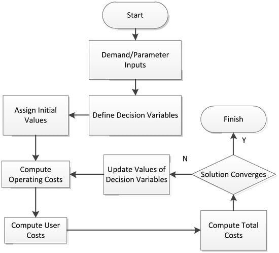
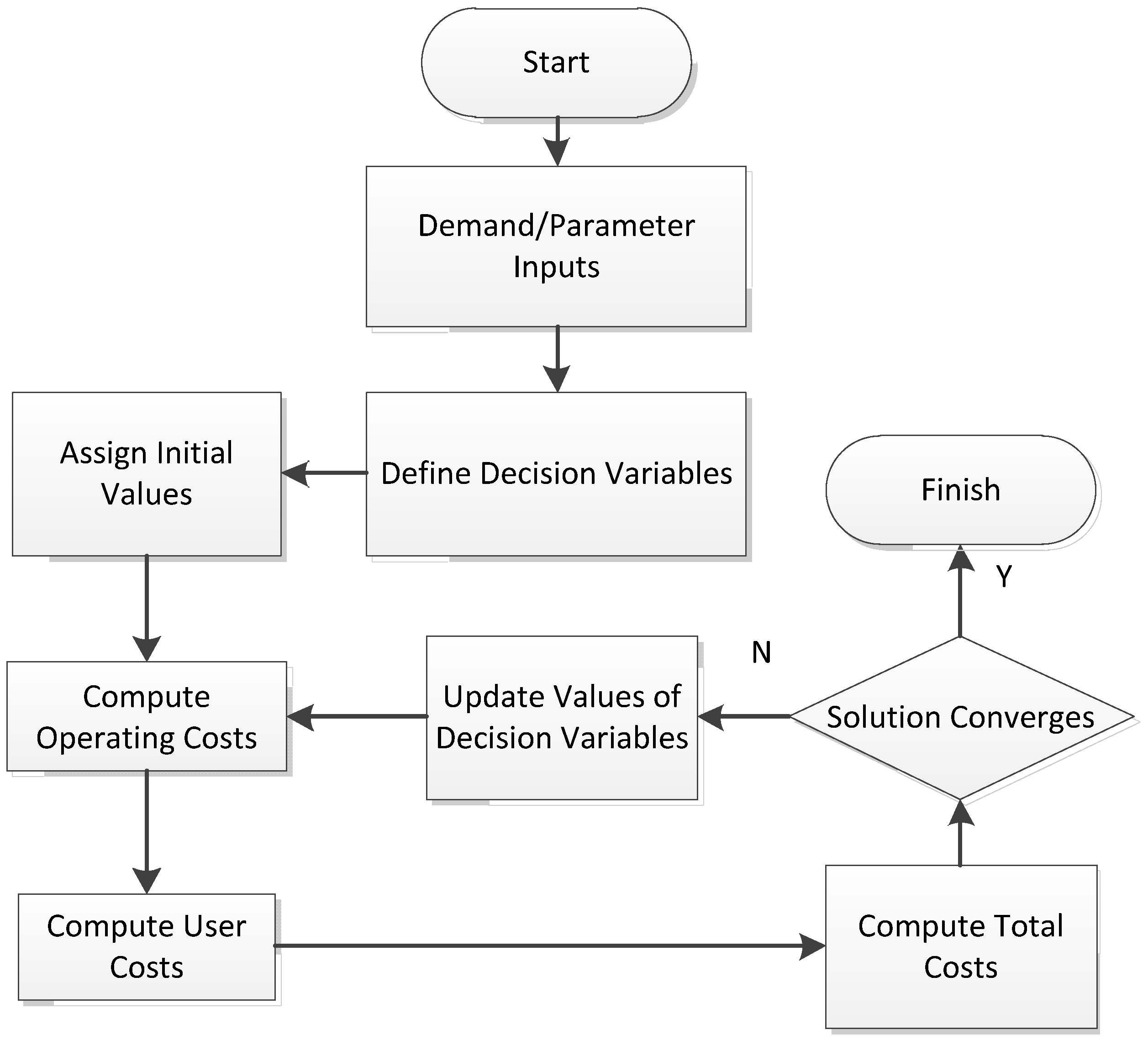
The optimization model in the previous section is non-linear. A solution algorithm for the optimization model is required to solve the problem and obtain the optimum solution. Thus, an exhaustive search method was selected. We used the genetic algorithm to determine the optimum transit route capacity $n_i^{\ast }$ and $n_{ji}$. The total cost of transit system is used as the fitness. If the individual satisfies all the constraints, the bus assignment process of the optimal strategy is carried out for each individual to determine the corresponding fitness value, calculate the optimal solution under the two objective functions, and select the minimum value as the final solution. Figure 1 illustrates the solution algorithm for the above objective function.

Figure 1. Solution algorithm.

4. Numerical Analysis

In order to prove that the proposed method can efficiently minimize the cost, we solve a numerical example and compare the cost of this method in multi bus size program. In addition, we analyze sensitivity to important input parameters. In the following sections, a numerical case study and sensitivity analyses are given.

4.1. Base Case

4.1.1. Inputs Values

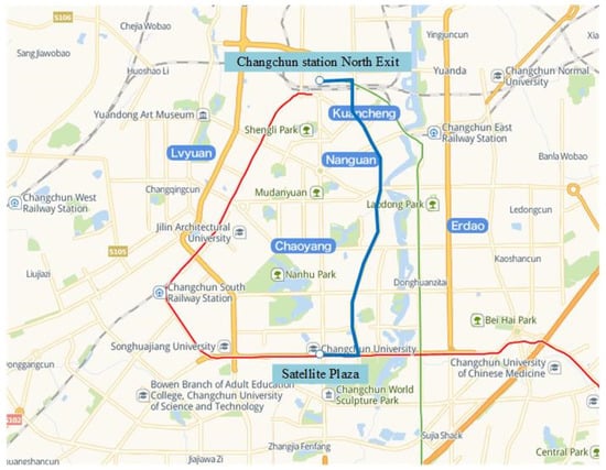
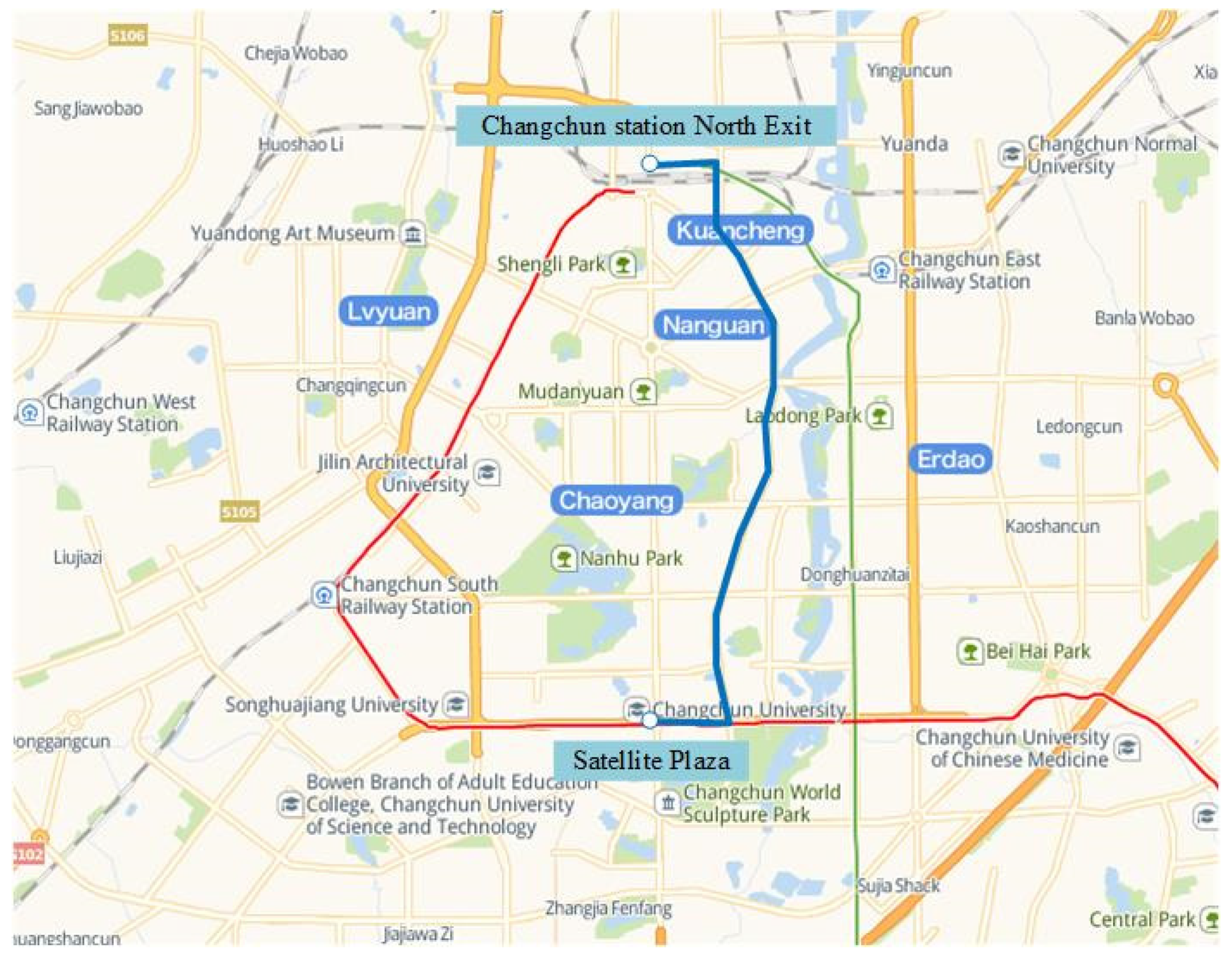
In the base numerical case, we take a bus line which is shown in Figure 2 in Changchun as an analysis object. The current bus model of the line is size 2, 30 vehicles. The number of vehicles operating during period 1 and 2 is 30 and 12 respectively, and the other required input parameters are presented in Table 1.

Figure 2. The bus line map.

Table 1. Related information on bus lines.

Parameter	Unit	Numerical Value (i = 1, 2, 3, 4, 5, 6 or j = 1, 2)
$q_i$	pax/bus	30, 60, 90, 120, 150, 180
$c{f}_i$	¥/h/bus	15, 24, 32, 36,37, 42
$c{k}_i$	¥/km	0.49, 0.71, 0.82, 1.04, 1.22, 1.40
$Q_j$	pax/h	15,000, 20,000
$Q_{j,peak}$	pax/h	2000, 500
$t{p}_j$	min	240, 600
$v_j$	km/h	15, 20
${\eta }_j$	1	1.3, 0.7
$c_p$	¥/h	15
$\phi$	¥/h	25
$h_{\max }$	min	20
$h_{\min }$	min	2
$L_r$	km	10
$\alpha$	1	0.5
$\beta$	1	0.5

4.1.2. Results of Base Case Study

The detailed results are shown in Table 2 (PCP method), including vehicle sizes and number, optimal headways, and corresponding costs. After the optimization of transport capacity, size 1, 2 and 6 of vehicles were selected and the number of vehicles decreased. The optimization results show that the total costs (TC) were reduced by 14.48%. Among them, the user costs (UC) decreased by 30.38% and the operator costs (OC) increased by 4.18%. Rolling costs (CK) and CP increased by 51.70% and 38.33% respectively, and CF decreased by 17.10%. This result shows that operating multiple sizes of buses can reduce the total cost in the case of significant demand changes.

Table 2. Optimization results of base case.

Parameter	Unit	Value
		Before Optimization	After Optimization	Savings (%)
$n_i^{\ast }$	bus	$n_2^{\ast }$ = 30	$n_1^{\ast }=20,n_2^{\ast }=2,n_6^{\ast }$ = 6	/
$n_{ji}$	bus	$n_{12}=30,n_{22}$ = 12	$n_{11}=20,n_{12}=2,n_{16}=6,n_{21}=20,n_{22}$ = 2	/
$h_j$	min	$h_1=2.5,h_2$ = 5.0	$h_1=2.9,h_2$ = 2.8	/
TC	¥/day	21,808.71	18,651.00	14.48
UC	¥/day	11,775.00	8197.89	30.38
OC	¥/day	10,033.71	10,453.11	−4.18
CK	¥/day	1284.27	1948.27	−51.70
CP	¥/day	2257.92	3123.46	−38.33
CF	¥/day	6491.52	5381.38	17.10

4.2. Sensitivity Analysis

In this section, a sensitivity analysis reveals the role played by various important input elements and show how the total cost and other optimized characteristics change from the baseline value, and how they change in different alternatives.

4.2.1. Cost Weight

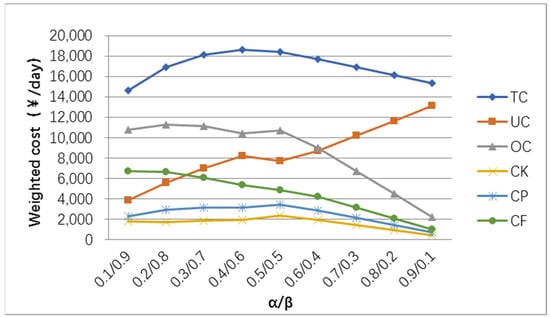
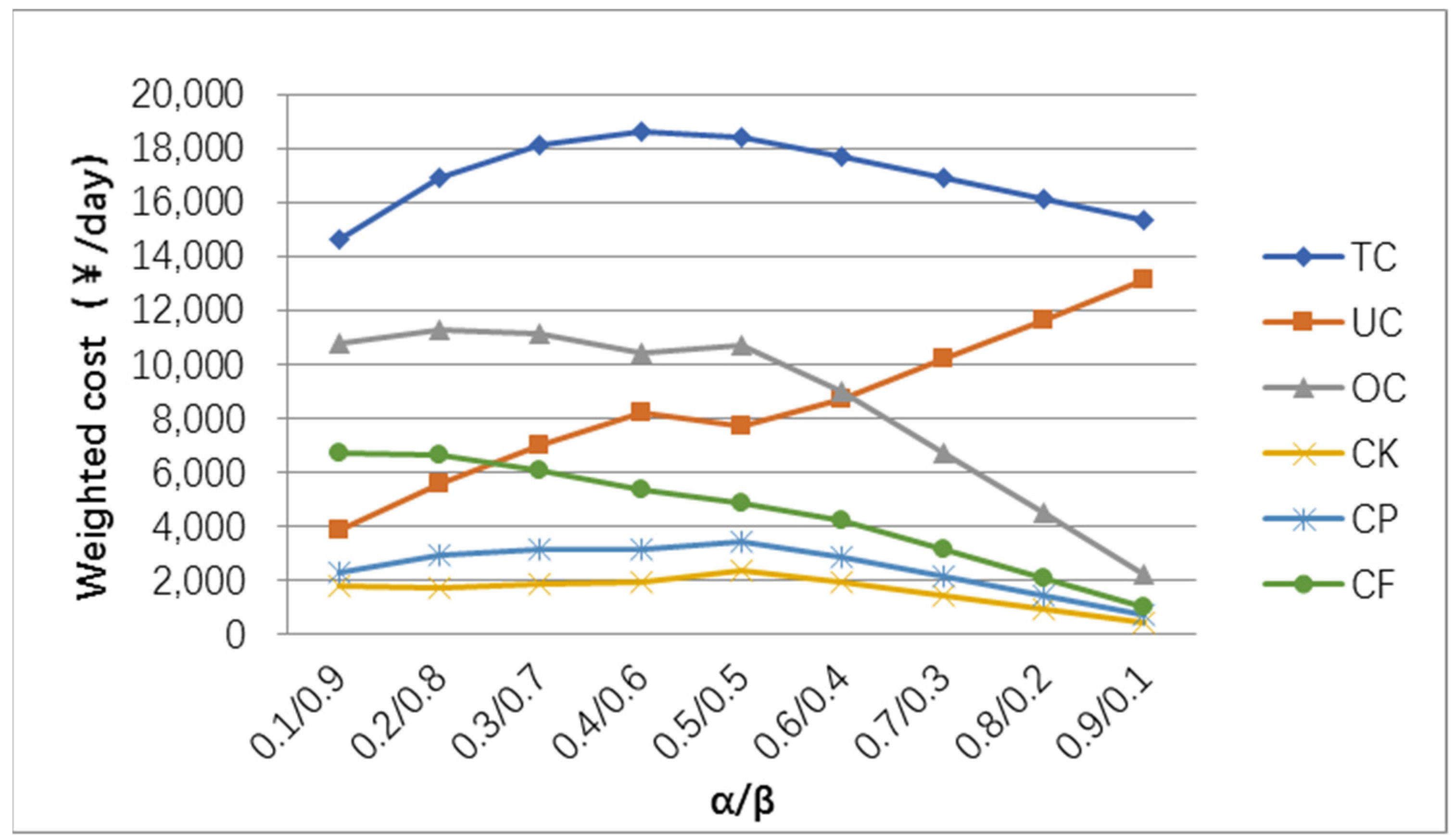
The cost weight indicates the importance to the user cost and operator cost, and the parameter $\alpha$ also reflects the change of passenger volume $Q_j$ and unit waiting time value $\phi$ to a certain extent. For parameter $\alpha$, Figure 3 shows relevant weighted cost variations. The sensitivity analysis results in Figure 1 show that with the increase of $\alpha$, OC, CK, CP and CF all showed a decreasing trend, but UC showed an increasing trend. TC first increased and then decreased. Moreover, $\alpha$ = 0.4 is the inflection point of TC and UC, and $\alpha$ = 0.5 is the inflection point of OC, CP and CK.

Figure 3. Weighted cost variations with parameter.

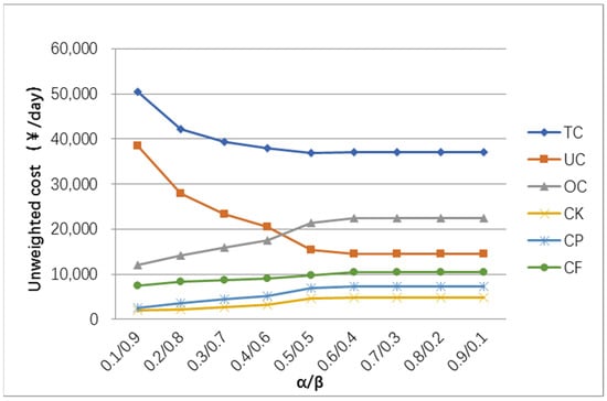
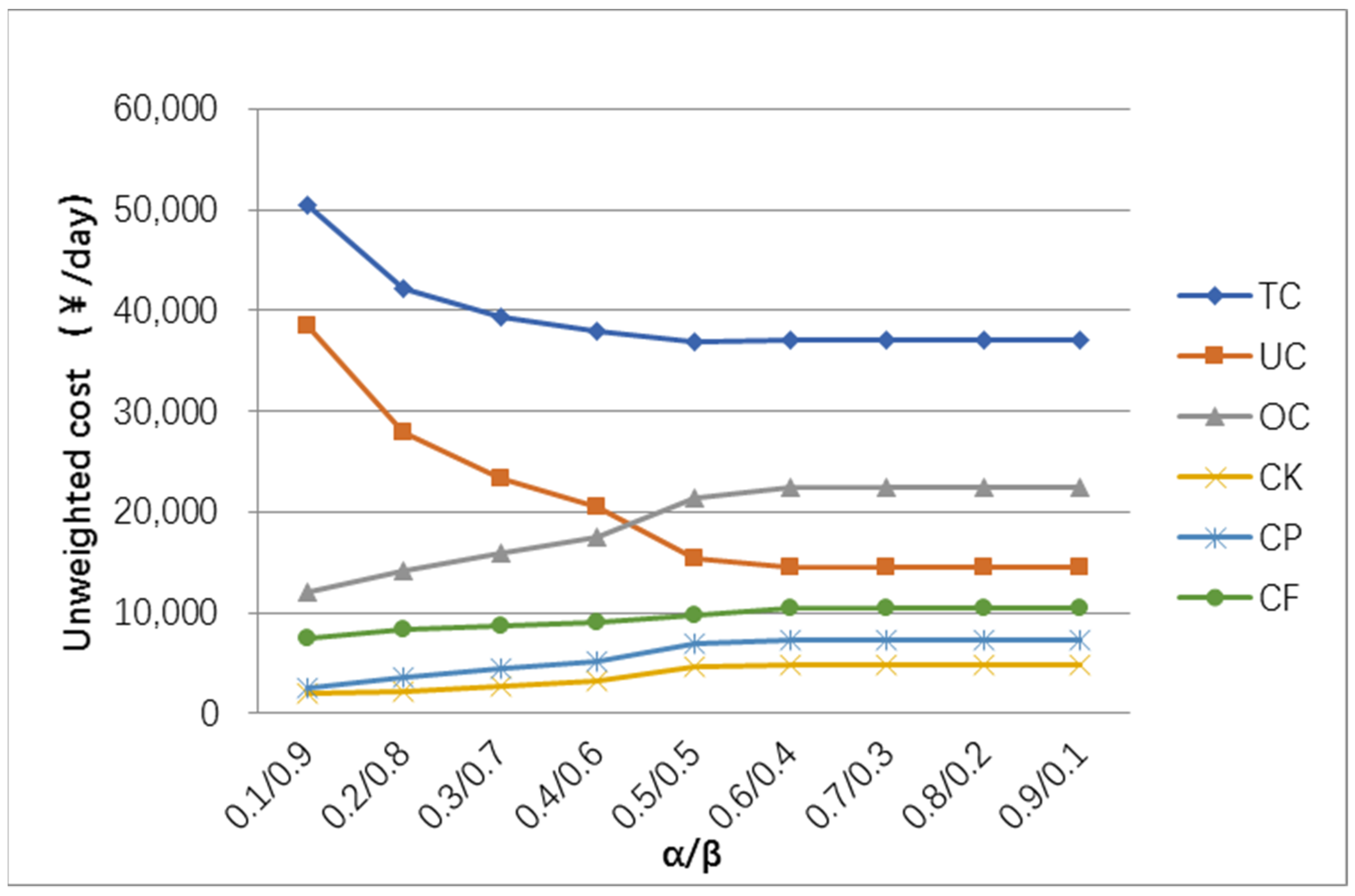
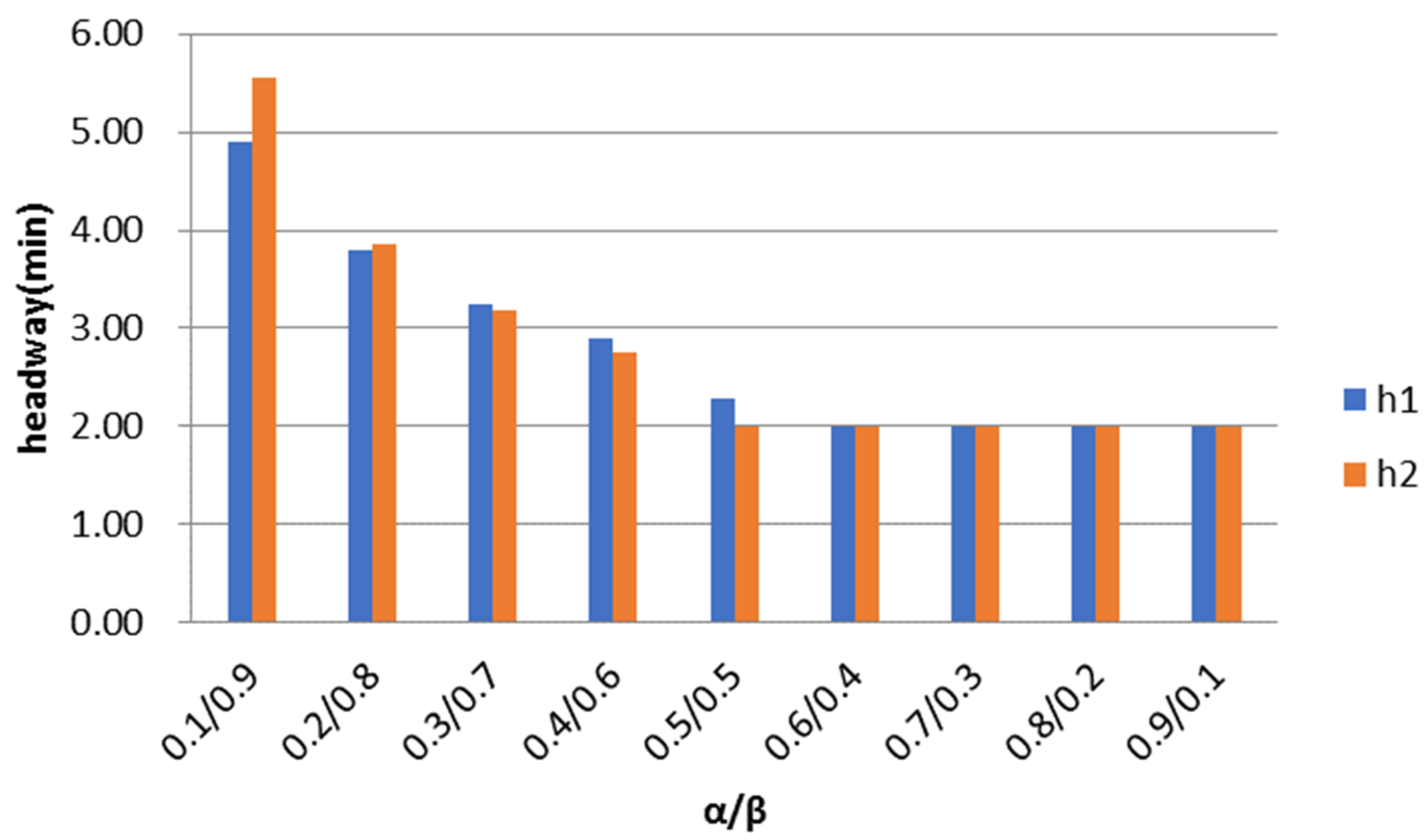
Figure 4 shows relevant unweighted cost variations. It shows that with the increase of $\alpha$, OC, CK, CP and CF all showed an increasing trend, but TC and UC showed a decreasing trend. $\alpha$ = 0.2 is the inflection point of TC, $\alpha$ = 0.5 is the inflection point of UC, OC, CK, CP, CF, when $\alpha$ > 0.5, the unweighted cost items tend to be stable. The increase of parameter $\alpha$ is equivalent to increasing passenger flow or waiting cost. At this time, the frequency of departure should be increased, the interval of headway should be reduced, as shown in Figure 5, and the cost of passengers is reduced and the total cost should be minimization at the end, but the operation cost will increase accordingly.

Figure 4. Unweighted cost variations with parameter $\alpha$.

Figure 5. Headway variations with parameter $\alpha$.

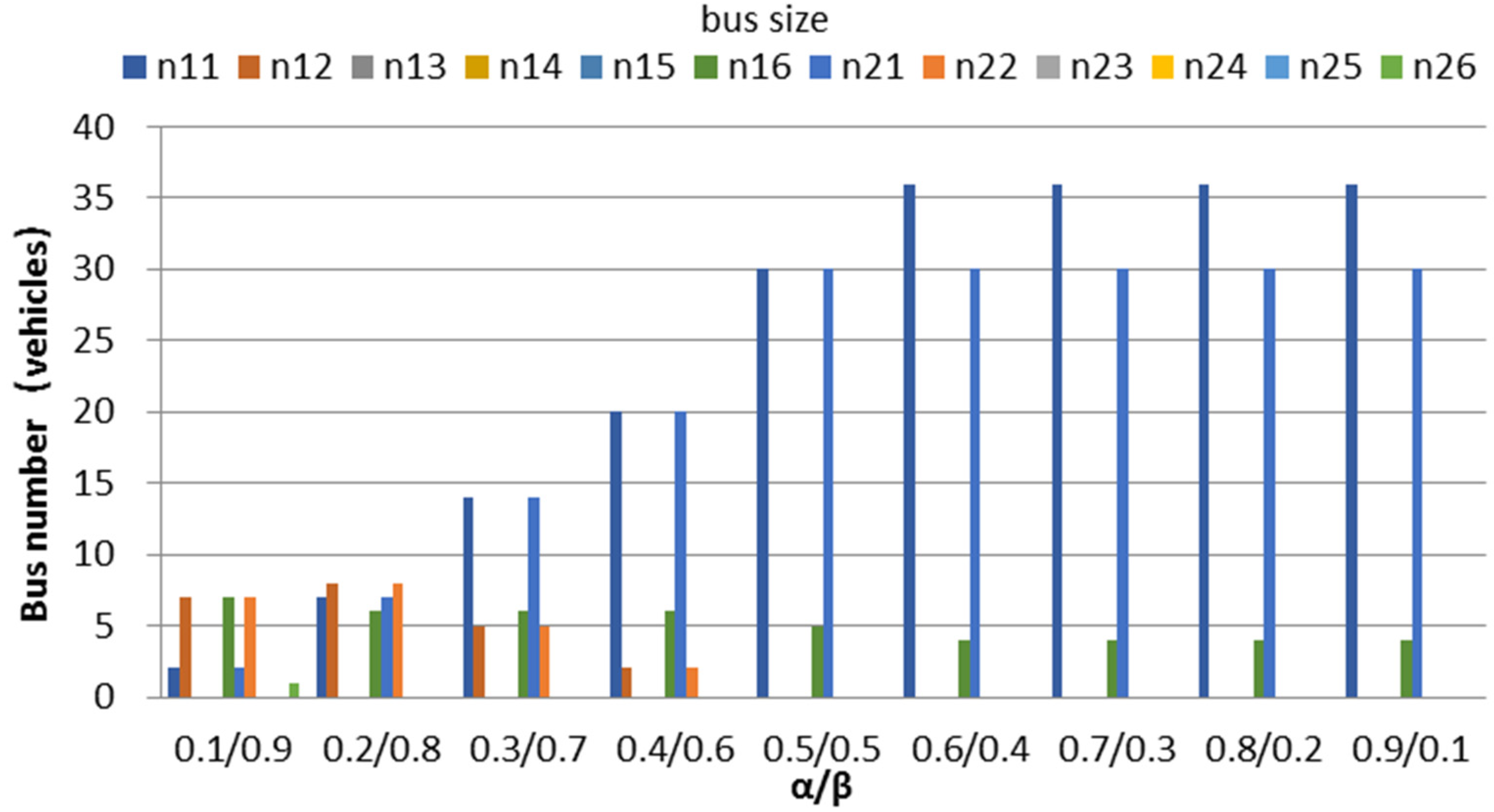
Figure 6 shows the number of different bus size variations. It shows that when $\alpha$ is smaller, the types of vehicle types are abundant. With the increase of $\alpha$, the vehicle types become more and more single, and the number of size 1 increases. When $\alpha <0.5$ size 1, 2 and 6 (Transport capacity is 30, 60, 180, respectively.) are put into use, and $n_i^{\ast }$ = $n_{1i}$. When $\alpha \ge 0.5$, size 1 and 6 are put into use, of which size 1 is far more than vehicle 6, and $n_i^{\ast }$ = $n_{1i}$. Because of the increase of passenger cost and weight, small vehicles can be used to reduce the departure interval, so as to reduce the user cost.

Figure 6. Number of different bus size variations with parameter $\alpha$.

4.2.2. Optional Bus Size

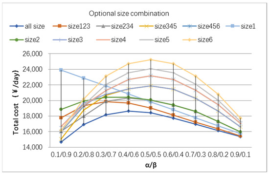
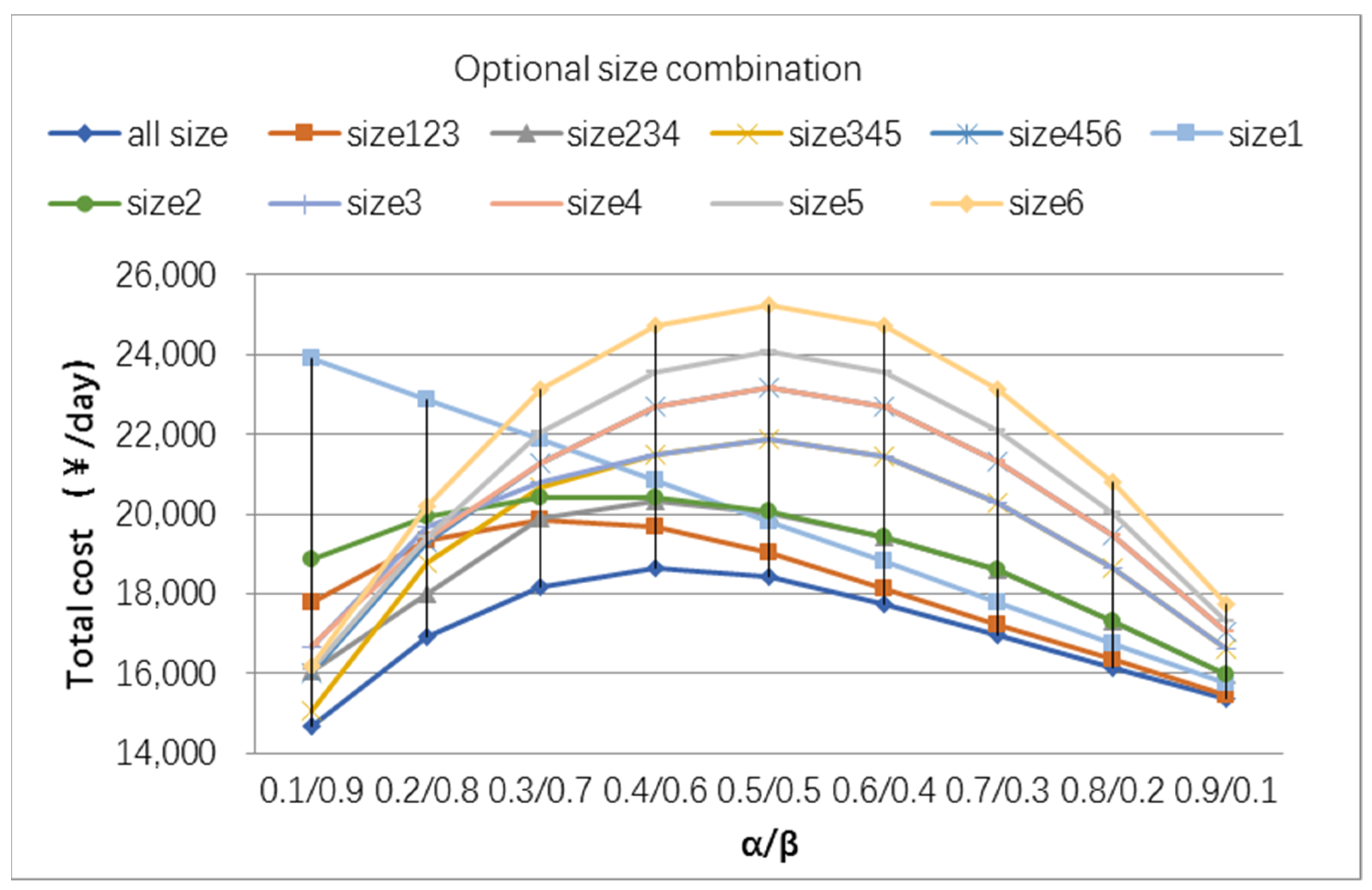
We divided the optional vehicle size into 11 groups. According to the optimization model, we can determine the optimal vehicle type and quantity and calculated the related costs of transport capacity scheme in each group. Figure 7 shows that, except for size 1, the total cost of other optimization results increases first and then decreases. Regardless of the value of $\alpha$, all size has the lowest cost. When $\alpha$ < 0.2, the cost of all size, size 5 and size 345 is lower, which is a better combination. When $\alpha$ > 0.5, the cost of all size, size 123, and size 1 is lower, which is a better combination. Because of the given passenger flow demand and minimum headway constraints, only size 1 cannot meet the transport demand, that is, if only size 1 of the vehicle is put into circulation, the headway based on the number of launch vehicles is less than the given lower limit of headway. When $\alpha \le 0.2$, there is no obvious change regulation in the total cost of the schemes. When $\alpha >0.2$, the total cost of multi-bus-size groups is less than that of a single-size vehicle, and the total cost of the small vehicle group is smaller than that of the medium and large vehicle scheme group.

Figure 7. Total cost variations with different optional bus size groups.

4.2.3. Cross-Section Passenger Volume

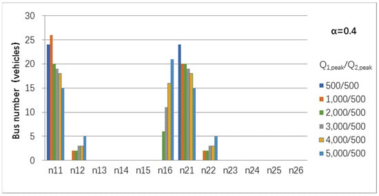
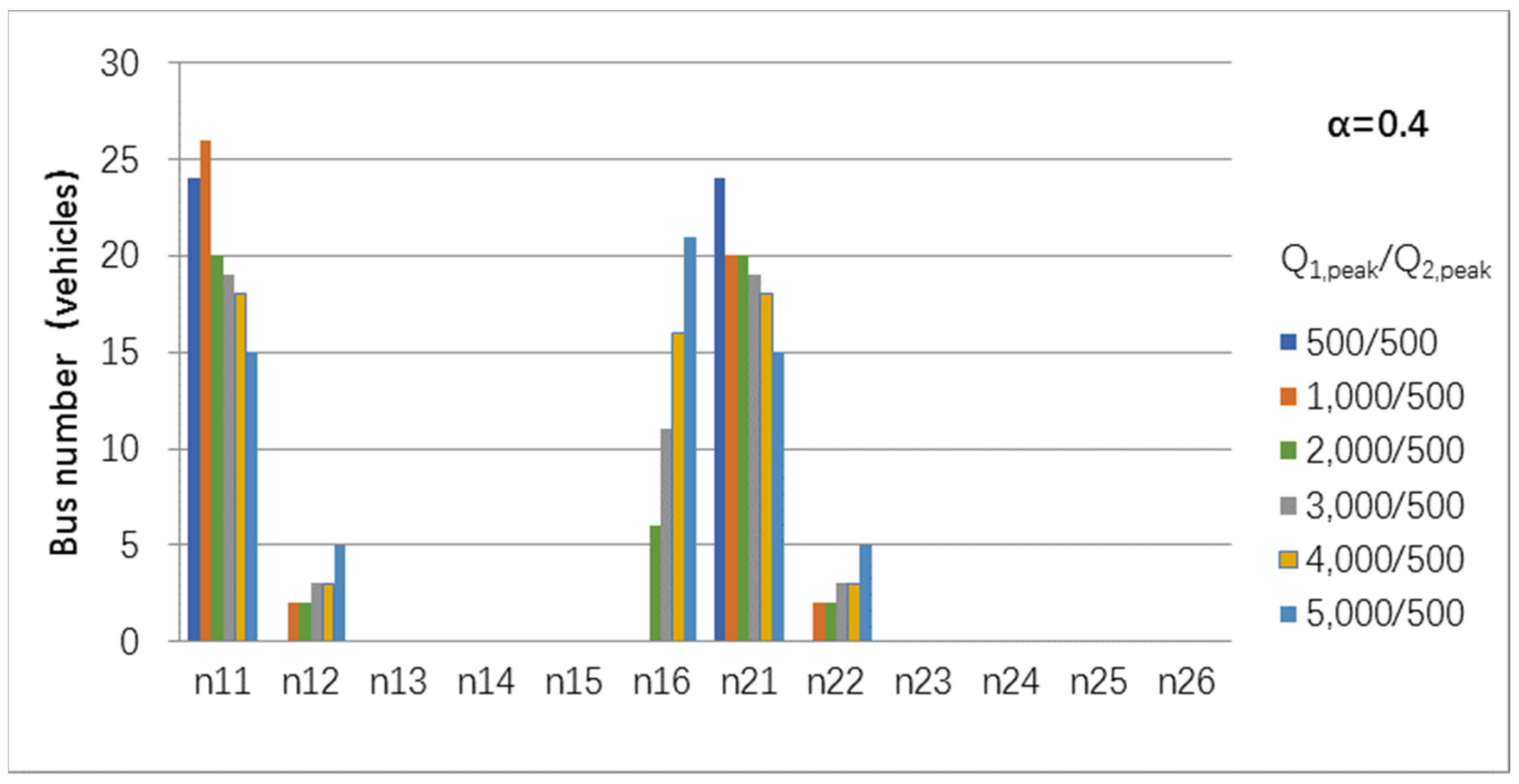
Cross-section passenger volume $Q_{j,peak}$ is important in this study because it affects the optimized number and size of buses and related cost. In the case of $\alpha =0.4$, the impact of $Q_{1,peak}$ changes on vehicle configuration $n_{ji}$ is analyzed, as shown in Figure 8. It shows that in the case of passenger volume $Q_j$ unchanged, with the increase of $Q_{1,peak}$, the vehicle number of size 1 gradually decreased, and number of size 2 and 6 increased gradually in period 1. Within period 2, the vehicle number of size 1 gradually decreased, and number of size 2 gradually increased. With the increase of cross-section passenger volume $Q_{1,peak}$, the minimum system cost can be obtained by investing in larger size vehicles.

Figure 8. Number of different bus size variations with parameter $Q_{1,peak}$.

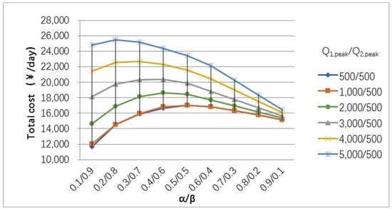
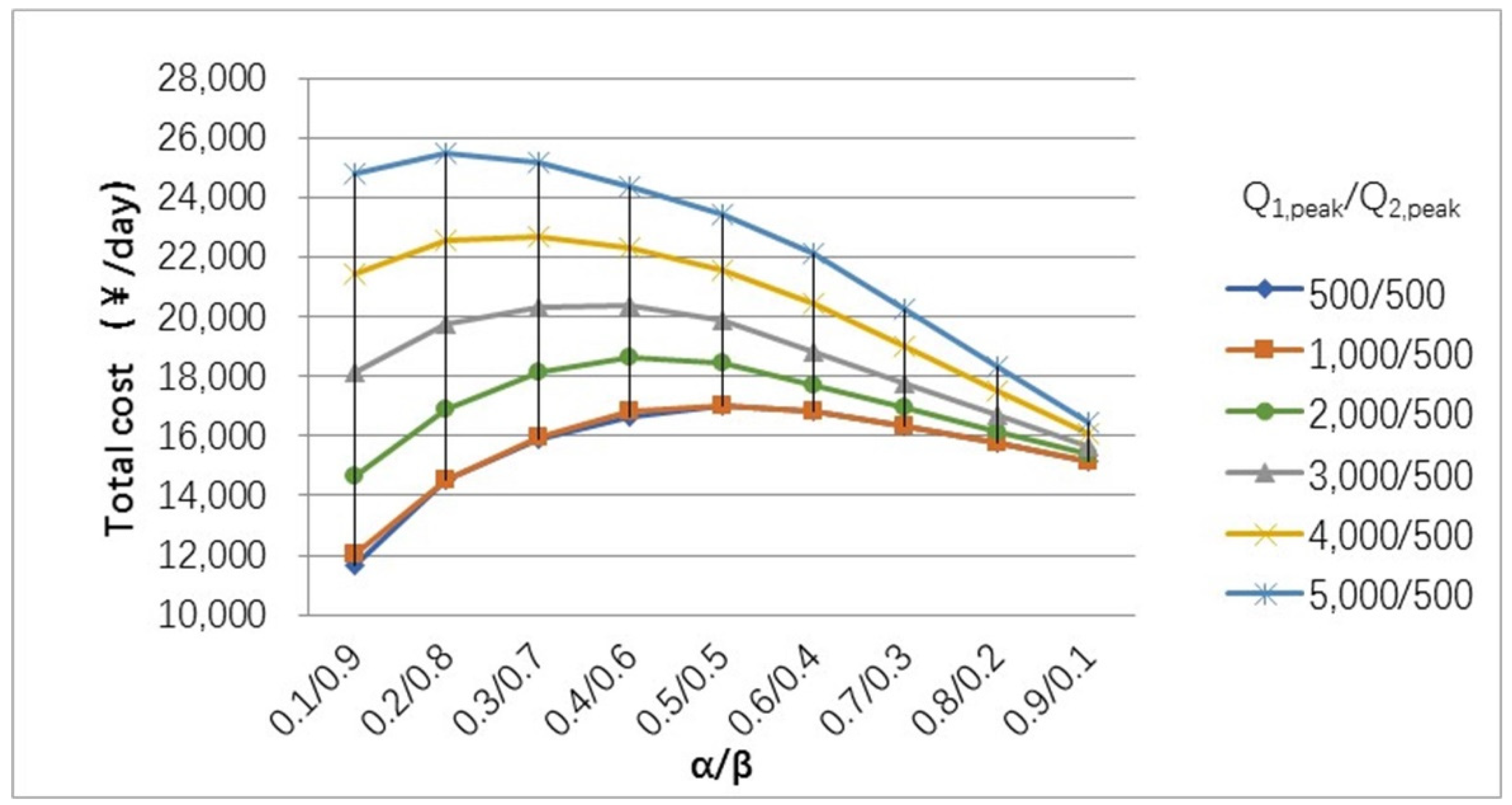
Total cost variations with parameter $Q_{j,peak}$ are shown in Figure 9. It shows that all cost curves are increased first and then decreased with parameter $\alpha$. For each $\alpha$ value, with the increase of $Q_{1,peak}$, the total cost gradually increases for increasing of the number vehicles invested; with the increase of $\alpha$, the total cost gap of the scheme gradually decreases due to the convergence of vehicle schemes.

Figure 9. Total cost variations with parameter $Q_{1,peak}$.

5. Conclusions

The primary purpose of this paper is to minimize the bus line cost by optimizing the vehicle type and quantity considering multi-bus-size. User cost and operation cost are considered in the proposed model objectives. Two methods are proposed to calculate the headway. According to the applicable conditions of the two methods, the scheme with the smallest target value is selected as the optimal solution in the numerical analysis. Then a base numerical case study and sensitivity analyses are presented to verify the validity of the model. The numerical examples shows that the multi size bus optimization can reduce the total cost, especially the user cost. Sensitivity analysis shows that weight has a greater impact on cost, and $\alpha$ = 0.2 and $\alpha$ = 0.5 are decision turning points. When bus line passenger flow or waiting time value is increased, more vehicles should be properly allocated to reduce the departure intervals, and the cost reduction of the users is greater than the operating cost, then the total cost of the system should be minimized. When the passenger flow is small, it is suitable to invest in the car with a smaller size. When the passenger flow is large, restricted by the lower limit of the headway, the combination of the smaller and larger size bus is more conducive to reducing the total cost of the system. When the passenger flow is increased to a certain extent, the more flexibly the vehicle size can be chosen, the more the system cost can be minimized by the rational allocation of the transport capacity, and the smaller size vehicle is more beneficial to reduce the cost of the system. The maximum cross-section passenger flow in each period directly affects the transport capacity of each period. With the increase of maximum cross-section passenger flow, the number of small cars gradually decreases, and the number of larger cars gradually increases. Under the same passenger flow of the bus line, the smaller the maximum cross-section passenger flow is, the smaller the system cost is, that is, the balanced passenger flow demand is beneficial to reduce the system cost. Then, the smaller the difference between total passenger flow and maximum cross-section passenger flow, the more obvious the trend of system cost reduction. We will incorporate uncertain demand and instability of vehicle operation in our future work. In this paper, only the multi-model vehicle distribution of a single bus line is considered, and it can also be used to solve the multi-model vehicle distribution problem of the regional bus network, which means that it is not only a single line, but the capacity can be shared. Besides this, we will consider multiple bus lines belong to the bus company and optimize the total fleet size serving different bus lines.

References

- Walters, A.A. Externalties in urban buses. J. Urban Econ. 1982, 11, 60–72. [Google Scholar] [CrossRef] [Scilit]
- Glaister, S. Bus deregulation, competition and vehicle size. J. Transp. Econ. Policy 1986, 20, 217–244. [Google Scholar]
- Oldfield, R.H.; Bly, P.H. An analytic investigation of optimal bus size. Transp. Res. Part B Methodol. 1988, 22, 319–337. [Google Scholar] [CrossRef] [Scilit]
- Lee, K.K.; Kuo, S.H.F.; Schonfeld, P.M. Optimal mixed bus fleet for urban operations. Transp. Res. Rec. 1995, 1503, 39–48. [Google Scholar]
- Fu, L.; Ishkhanov, G. Fleet size and mix optimization for paratransit services. Transp. Res. Rec. 2004, 1884, 39–46. [Google Scholar] [CrossRef] [Scilit]
- Jara-Díaz, S.R.; Gschwender, A. The effect of financial constraints on the optimal design of public transport services. Transportation 2009, 36, 65–75. [Google Scholar] [CrossRef] [Scilit]
- Dell’Olio, L.; Ibeas, A.; Ruisánchez, F. Optimizing bus-size and headway in transit networks. Transportation 2012, 39, 449–464. [Google Scholar] [CrossRef] [Scilit]
- Kim, M.; Schonfeld, P. Conventional, flexible and variable-type services. J. Transp. Eng. 2012, 138, 263–273. [Google Scholar] [CrossRef] [Scilit]
- Ceder, A.; Hassold, S.; Dano, B. Approaching even-load and even-headway transit timetables using different bus sizes. Public Transp. 2013, 5, 193–217. [Google Scholar] [CrossRef] [Scilit]
- Ibeas, A.; Alonso, B.; dell’Olio, L.; Moura, J.L. Bus Size and Headways Optimization Model Considering Elastic Demand. J. Transp. Eng. 2014, 140, 370–380. [Google Scholar] [CrossRef] [Scilit]
- Ibarra-Rojas, O.J.; Delgado, F.; Giesen, R.; Muñoz, J.C. Planning, operation, and control of bus transport systems: A literature review. Transp. Res. Part B Methodol. 2015, 77, 38–75. [Google Scholar] [CrossRef] [Scilit]
- Jara-Díaz, S.; Fielbaum, A.; Gschwender, A. Optimal fleet size, frequencies and vehicle capacities considering peak and off-peak periods in public transport. Transp. Res. Part A Policy Pract. 2017, 106, 65–74. [Google Scholar] [CrossRef] [Scilit]
- Vazquez-Abad, F.J.; Fenn, L. Mixed optimization for constrained resource allocation, an application to a local bus service. In 2016 Winter Simulation Conference (WSC); IEEE: Washington, DC, USA, 2016; pp. 871–882. [Google Scholar]
- Li, L.; Lo, H.K.; Xiao, F.; Cen, X. Mixed bus fleet management strategy for minimizing overall and emissions external costs. Transp. Res. Part D Transp. Environ. 2018, 60, 104–118. [Google Scholar] [CrossRef] [Scilit]
- Liang, S.; Ma, M.; He, S. The Impact of Bus Fleet Size on Performance of Self-equalize Bus Headway Control Method. Proc. Inst. Civ. Eng.-Munic. Eng. 2018, 172, 246–256. [Google Scholar]
- AlKheder, S.; Savsar, M.; AlRukaibi, F.; Zaqzouq, A. Optimal Fleet Size for Kuwait Public Transport Company Based on Integer Linear Programming. In Proceedings of the 2019 IEEE Intelligent Transportation Systems Conference (ITSC), Auckland, New Zealand, 27–30 October 2019; pp. 981–986. Available online: http://ieeexplore.ieee.org/document/8917210 (accessed on 2 October 2021).
- Liang, S.; Ma, M.; He, S. Multiobjective optimal formulations for bus fleet size of public transit under headway based holding control. J. Adv. Transp. 2019, 2019, 2452348. [Google Scholar] [CrossRef] [Scilit]
- Tian, Q.; Lin, Y.H.; Wang, D.Z. Autonomous and conventional bus fleet optimization for fixed-route operations considering demand uncertainty. Transportation 2020, 48, 2735–2763. [Google Scholar] [CrossRef] [Scilit]
- Jara-Díaz, S.; Fielbaum, A.; Gschwender, A. Strategies for transit fleet design considering peak and off-peak periods using the single-line model. Transp. Res. Part B Methodol. 2020, 142, 1–18. [Google Scholar] [CrossRef] [Scilit]
- Sun, Q.; Chien, S.; Hu, D.W.; Chen, G.; Jiang, R.S. Optimizing Multi-Terminal Customized Bus Service with Mixed Fleet. IEEE Access 2020, 8, 156456–156469. [Google Scholar] [CrossRef] [Scilit]
- Jiang, X.H.; Ma, J.X. Mixed Scheduling Model for Limited-Stop and Normal Bus Service with Fleet Size Constraint. Information 2021, 12, 400. [Google Scholar] [CrossRef] [Scilit]
- Salicrú, M.; Fleurent, C.; Armengol, J.M. Timetable-based operation in urban transport: Run-time optimisation and improvements in the operating process. Transp. Res. Part A Policy Pract. 2011, 45, 721–740. [Google Scholar] [CrossRef] [Scilit]
Publisher’s Note: MDPI stays neutral with regard to jurisdictional claims in published maps and institutional affiliations. |
© 2021 by the authors. Licensee MDPI, Basel, Switzerland. This article is an open access article distributed under the terms and conditions of the Creative Commons Attribution (CC BY) license (https://creativecommons.org/licenses/by/4.0/).