Computational Valuation Model of Housing Price Using Pseudo Self Comparison Method

Abstract

Hedonic pricing method (HPM), which is commonly used for estimating real estate property values, considers the property’s internal and external characteristics for its valuation. Despite its popularity, however, the method lacks the mechanism that directly reflects the target property’s price fluctuation and the real estate market’s volatility over time. To overcome these limitations, we propose Pseudo Self Comparison Method (PSCM), which reduces the real estate valuation problem to finding a pseudo self, which is defined as a housing property that can most closely approximate the characteristics of the target housing property, and adjusting its previous transaction price to be in sync with the real estate market change. The proposed PSCM is tested for two scenarios in which the volatility of the real estate market varies greatly, using the transaction data compiled from Seoul, the capital of South Korea, and its surrounding region, Gyeonggi. The study results show almost five times lower estimation errors when predicting housing transaction prices using the PSCM compared to the HPM in both scenarios and in both areas. The proposed method is particularly useful for mass valuation of apartments or densely located housing units.

1. Introduction

Research has been extensively conducted to accurately estimate actual housing transaction prices while the importance of accurate valuation has become apparent in recent years. As previous research has found [1], the housing prices perform a role of an early warning signal for financial crisis. In addition, due to the significant effect of volatility in real estate value on the national economy [2], correctly assessing the value of real estate based on the actual housing transaction price is crucial. Prior studies [3,4] warned that insufficient data and analysis would lead to the banks’ underestimating the financial market loan risk, fostering a false sense of prosperity and a consequent economic collapse. Thus, the inaccurate valuation of real estate can trigger a collective panic by the investors, causing losses in financial institutions and increasing economic danger [5].

A widely known example of a financial crisis caused by an inaccurate real estate valuation is the subprime mortgage crisis [6] that occurred in 2008. The subprime mortgage crisis started with the United States’ policy to boost the stagnant economy in an economic downturn that incentivized mortgage loans with low interests, which led to an increase in housing prices. The trend of rising housing prices, combined with the low mortgage interest, guaranteed the financial institutions a safety net even when a borrower filed for bankruptcy. This allowed for more lenient loan regulations and valuations of real estate. These securitized subprime mortgage loans were given investment-grade ratings, guaranteeing a higher return, and amplifying the volume of transactions. However, as the housing bubble started to burst in 2004 when the low-interest policy ended, low-income borrowers were unable to make payments as the subprime mortgage loan interest rose. Consequently, numerous financial institutions that had purchased securitized subprime mortgage loans could not recover their loans and suffered massive losses. This process resulted in the insolvency of many companies, which led to a series of bankruptcies of large U.S. financial and security firms.

As aforementioned, an accurate estimation of the housing transaction price is crucial to preventing an economic crisis on national and societal levels and providing an effective investment opportunity on a personal level. Moreover, from the perspective of long-term urban planning, appropriate tax estimation achieved through accurate valuation of massive real estate properties can invoke balanced and sustainable urban development [7]. For accurate valuation, many applications have been developed and utilized [8,9]; among them, the key element is the Hedonic Pricing Method (HPM) [10]. The HPM, a commonly used method to estimate the value of real estate properties, parametrizes the internal characteristics (structural or physical characteristics) and external characteristics (neighborhood or environmental characteristics) of a house to assess its value. This method considers those characteristics as independent variables and the housing transaction price as the dependent variable. The relationship, or the degree of influence, between these variables is assumed to be linear to determine the housing transaction price intuitively.

Given that the purpose of a house is not limited to residence and that it can be used as an investment asset for profits, the housing price can be affected by many external forces such as economic fluctuations, government regulations, and future development plans. Further, the housing transaction price is determined by considering not only internal and external characteristics of a house but also many other elements of changes in the real estate market such as the price changes of comparable houses in the neighborhood and current mortgage terms. In addition, house price changes are different from other financial assets (e.g., stock, gold, oil, bitcoin), and they are different from one area to another. Despite its popularity, however, the HPM lacks the mechanism that directly reflects the target property’s price fluctuation and the real estate market’s volatility over time. To overcome these limitations, Kim et al. [11] proposed a new method based on the Sales Comparison Approach (SCA), which estimates the housing price from the selected comparable sales. Their method automatically selects comparable sales based on a set of predefined criteria and estimates the values of real estate properties on a mass scale. Going further, in this study, we propose Pseudo Self Comparison Method (PSCM), which reduces the real estate valuation problem to finding a pseudo-self, which is defined as a housing property that can most closely approximate the characteristics of the target housing property, and adjusting its previous transaction price to be in sync with the real estate market change. The method is more efficient than the Kim et al.’s approach, with comparable results (slight performance differences are due to the methodological artifacts of regression vs. machine learniang).

2. Related Work

This section introduces the hedonic pricing method, a common method in estimating the housing transaction price, and the sales comparison analysis, a popular practical method employing a different perspective to estimate the house prices.

2.1. Hedonic Pricing Method (HPM)

Freeman [12] argued that the value of real estate could reflect its structural, neighborhood, and environmental characteristics. Therefore, the value of housing can be expressed as its transaction price, for which the price function of house e can be established as follows:

$$H_e=H(S_1,\dots ,S_x,N_1,\dots ,N_y,E_1,\dots ,E_z)$$

(1)

where independent variables $S_x$, $N_y$, and $E_z$ are the structural, neighborhood, and the surrounding environmental or locational characteristics, respectively. Some examples of structural characteristics can include the number of rooms or bathrooms and the floor space of the real estate. Neighborhood characteristics can describe the residents living in the area, such as the educational quality of a nearby school. Environmental or locational characteristics can include air or water pollution levels and the accessibility of surrounding facilities.

Let $HX$ be the overall set of the independent variables ($S_x$, $N_y$, and $E_z$); then the relationship between the price estimation model (h) and the constituent variables is as follows:

$$h_i=h(H{X}_i,{\beta }_{hedonic},{\epsilon }_{hedonic})$$

(2)

where ${\beta }_{hedonic}$ is a parameter to be determined, ${\epsilon }_{hedonic}$ is the stochastic residual term, and $h_i$ is the estimated price of the ith house based on its hedonic characteristics $H{X}_i$.

The aforementioned variables are defined as the HPM features. The structural characteristics are categorized as internal factors because they represent the intrinsic characteristics of the house, and the neighborhood and the environmental and locational characteristics are categorized together as external factors because they represent extrinsic characteristics of the house.

The utilization of linear models in HPM makes it easy to interpret the relationships between the the variables, which also helps the model to be widely used to evaluate real estate prices [13,14,15,16], as well as in other fields of study. Hawkins and Habib [17] utilized HPM to analyze the factors affecting real estate prices in Toronto, Canada, where the community’s average income, the proximity to the central business district, and the population and employment density were determined as the significant factors. Xue et al. [18] used HPM to develop a new estimation model with an average $R^2$ score of 0.22. Research has been done on the methodology of HPM as well, where Francke and Van de Minnie [19] reported that the addition of mutually independent, random characteristics improved out-of-sample estimations of real estate prices. In other fields of study, HPM was employed to analyze the decision factors of the price of groceries (e.g., wine [20] and rice [21]), ticket prices of a ski lift [22], and a football match [23].

Recently, much research effort has gone into applying machine learning to improve the price estimation performance of HPM. In the aforementioned study conducted by Xue et al. [18], the use of RandomForest to develop a prediction model while retaining the variables increased the average $R^2$ score to at least 0.8. Alfaro-Navarro et al. [24] compared the effectiveness of different machine learning methods on hedonic-based regression models and showed that bagging and RandomForest performed better than the boosting or decision tree algorithms. While these studies show meaningful improvements compared to the traditional HPM, the relationships between the real estate variables and the estimated prices could not be traced due to the nature of machine learning.

2.2. Sales Comparison Approach (SCA)

2.2.1. Basic Concept

Sales Comparison Approach (SCA) [25], also known as Comparative Market Analysis (CMA) [26], is a traditional methodology widely used by real estate agents and appraisers to perform a valuation of real estate. To estimate the value of a real estate property, the SCA takes a sample of similar neighboring real estates that have been sold recently. This information is adjusted according to the time passed and the differences in attributes (i.e., variables) of the real estate properties. For this adjustment, the value can be quantified and corrected with methods such as percentage adjustment. The final adjusted price can be further accompanied by the estimation of a subjective value, depending on the personal knowledge and experience of a particular market.

This approach obeys the law of supply and demand of the market. Specifically, assuming no extraneous delays in construction, the consumer is assumed to opt to buy cheaper real estate when expecting similar benefits or convenience. Furthermore, the SCA requires an active real estate market that is both economically stable in the regional markets and predictably volatile on a national scale.

2.2.2. Formula

As mentioned previously, the SCA leaves room for the judgment of an appraiser to be reflected. Because it is challenging to express appraiser’s subjectivity as a formula, the existing study [27] compiled the formula according to the one-price assumption, without considering the appraiser’s subjectivity. This formula is expressed as follows:

• S = A ($1\times n$) vector of n indicated values of the particular subject property;
• P = A ($1\times n$) vector of the selling prices of n comparable properties;
• A = A ($1\times j$) vector of j adjustment factors;
• X = A ($j\times 1$) vector of the j property characteristics of the subject property;
• Z = A ($j\times n$) matrix of the j characteristics of the n comparable properties;
• I = A standard ($1\times n$) unit vector (all elements of I are 1).

$$S=P+A(XI-Z)$$

(3)

The difference between the subject property characteristic, X, and the comparable properties, Z, is corrected with an adjustment factor, A, and is added to the selling price of comparable properties, P, to calculate the average subject property price, S.

Despite these fundamental assumptions required, the SCA demonstrates a strong valuation capability and is widely employed in land appraisal [28], timberland valuation [29], and unmined mineral valuation [30].

3. Pseudo Self Comparison Method (PSCM)

In short, the Sales Comparison Approach (SCA) calculates the value of the target property by adjusting the nearby comparable sales based on the difference in characteristics. The SCA considers the hedonic characteristics such as the structural, neighborhood, and environmental/locational characteristics, as well as the market conditions and economic characteristics [31]. Furthermore, the usage and conditions of sale are considered necessary. In all, the SCA can be largely divided into the initial consideration of hedonic characteristics to search for comparable sales and the post-adjustment to the prices of the comparable sales by considering the overall characteristics. However, it has the limitation that the adjustment relies on the subjectivity of the appraiser, primarily manifested in selecting the comparable sales and estimating prices. The Pseudo Self Comparison Method (PSCM) is proposed to overcome this limitation of subjectivity in comparable sales selection, not to mention its clear advantage in cost and time for a large number of valuations.

3.1. The Definition of Pseudo Self

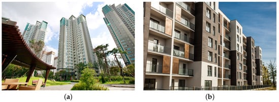
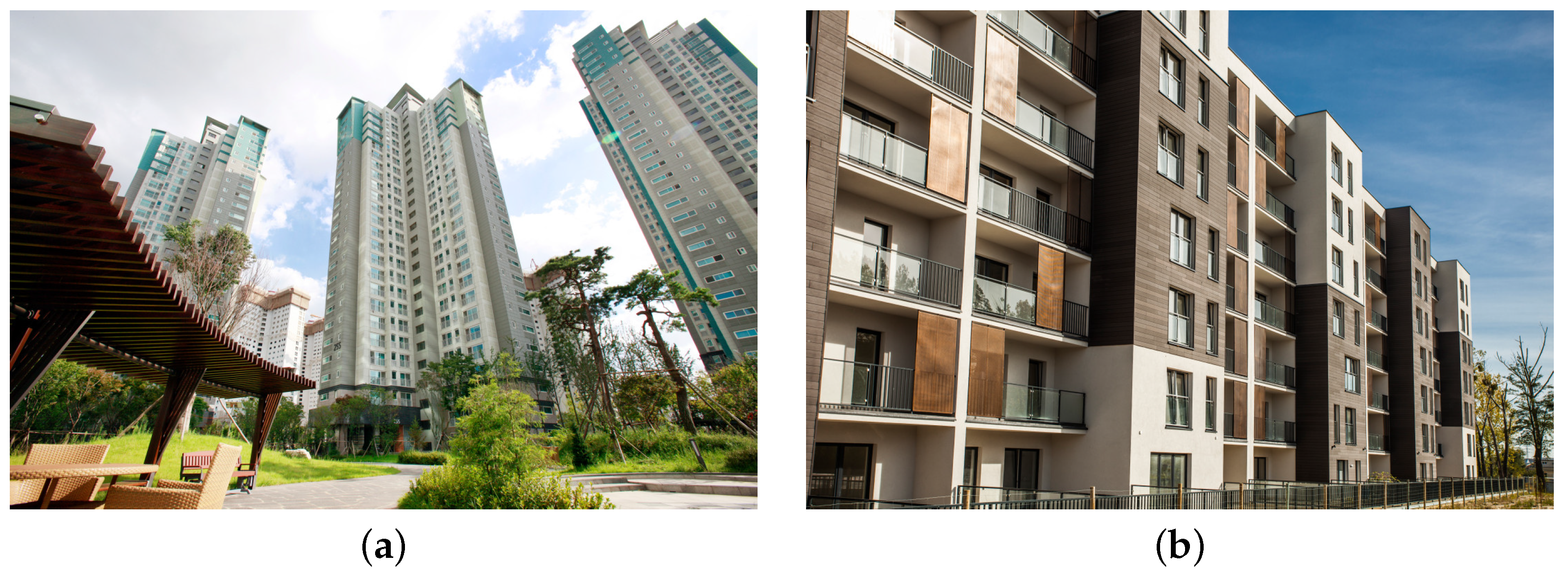
In our study context, Pseudo Self is defined as the housing property that can most closely approximate the characteristics of, particularly the price characteristic of, the target housing property. The word pseudo implies that it is a housing property different from the target. An example of pseudo self can be easily found within an apartment building, condominium complex, town house area, or other densely located housing units built in a similar style. Figure 1 presents some of these types of houses.

Figure 1. Examples of apartments and condominiums. (a) Apartments. (b) Condominiums.

3.2. Selection of Pseudo Self

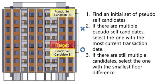
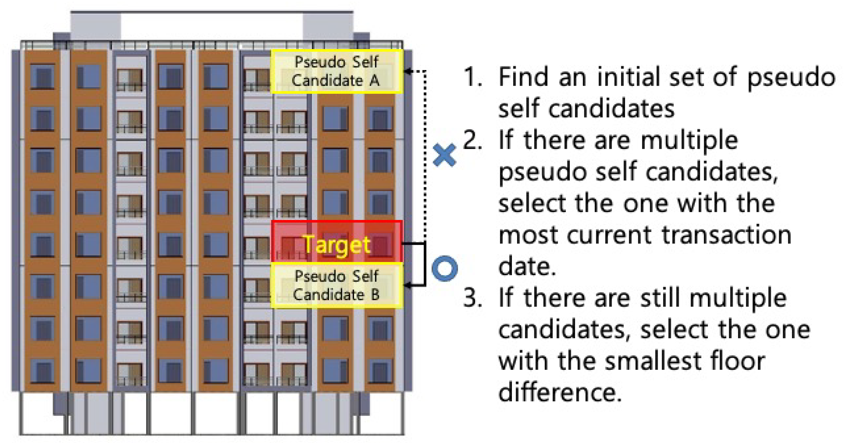
Although the concept of pseudo self can be applied to various housing settings, we selected apartment buildings as our study setting as apartments are the most popular residential housing type in Korea [11]. As illustrated in Figure 2, for a certain target apartment for which we want to predict its current market value, it is possible to have multiple pseudo self candidates, which have the same apartment size in the same apartment complex. Then, out of those candidates, we select the one with the most current transaction date so that we can use the most current market value of a comparable house. If there are still multiple pseudo self candidates, the information from the pseudo self at the closest floor to the target is selected.

Figure 2. Pseudo self section rule.

3.3. Pseudo Self Features

We utilize pseudo self’s previous transaction information in a similar way to the sales comparison approach. For every real estate property, we assume that its transaction price reflects the overall value of its hedonic characteristics up to that point and that the market and economic volatility determines its future transaction price. This assumption is due to the limitation of reflecting market and economic volatility using the hedonic characteristics and the desire to allow the volatility to take effect as its valuation needs to take account of the corresponding value change in the market over time.

Under these assumptions, the relationship between the desired transaction price and its constituting variables can be expressed as follows:

$$S_e=S(P{P}_1,\dots ,P{P}_j,M{C}_1,\dots ,M{C}_k)$$

(4)

where $P{P}_j$ is the previous transaction information of the pseudo self, and $M{C}_k$ is the market change. The previous transaction information includes the previous transaction price and adjustable factor. The market change includes the contextual change of the market, which indicates index differences since the previous transaction.

Let $PSX$ represent the full set of pseudo self characteristics ($P{P}_j$ and $M{C}_k$), and the relationship between the price estimation model s and the constituent variables is as follows:

$$s_i=S(PS{X}_i,{\beta }_{pscm},{\epsilon }_{pscm})$$

(5)

where ${\beta }_{pscm}$ is a parameter to be determined, ${\epsilon }_{pscm}$ is the random error variable due to the standard logistic distribution, and $s_i$ is the ith estimated price based on the PSCM features. Table 1 presents a summary of the features used by HPM and PSCM.

Table 1. The descriptions of the features.

Features	Types	Characteristics	Descriptions
HPM	Internal	Structural (S)	Physical attributes of the house
	External	Neighborhood/ Environmental (NE)	The neighborhood and environmental characteristics
PSCM	Internal	Previous price (PP)	Previous price of pseudo self
	External	Market change (MC)	Market changes that affect the house price

HPM: Hedonic Pricing Method, PSCM: Pseudo Self Comparison Method.

4. Experiments

4.1. Dataset

4.1.1. Target Cities and Periods

Cities

The apartment complex transaction data were compiled from the capital, Seoul, and its surrounding region, Gyeonggi. Apartment complexes are the most common form of housing, constituting 67.5% of all housing transactions in the fourth quarter of 2018 [32]. Seoul is known to have the highest population density in the world, along with significant price volatility due to the high demands for housing. Gyeonggi has a lower population density relative to Seoul, but the region has the highest population in South Korea. The 2018 population and density information for each area is presented in Table 2.

Table 2. The selected area information in 2018.

Region	Size [33]	Population [34]	Density [34]
Seoul	605.24	9705	16,034
Gyeonggi	10,187.79	13,031	1279
Unit	km${}^2$	1000 people	people/km${}^2$

Periods

Two scenarios were established by considering actual real estate conditions. The second half of 2018 showed a spike in real estate prices [35]. Taking advantage of this move, the first scenario, or the “Stable” scenario, used the real estate transaction data up to 2017 as training data and the first half of 2018 as evaluation data. The second scenario, or the “Rising” scenario, used the transaction data up to the first half of 2018 as training data and the second half of 2018 as evaluation data. Table 3 provides a summary of the two periods associated with each data set.

Table 3. The period of each scenario.

Scenario	Train	Test
Scenario 1 (Stable)	1 January 2010∼31 December 2017	1 January 2018∼30 June 2018
Scenario 2 (Rising)	1 January 2010∼30 June 2018	1 July 2018∼31 December 2018

4.1.2. Features

Transaction Price

The transaction prices of the apartment complexes in the two areas were taken from the “Transaction Price Open System” [36] provided by the Ministry of Land, Infrastructure, and Transport (MOLIT), South Korea. The transaction price, which is a dependent variable in this study, has a unit of 10,000 KRW. The volume of transaction data used in this study for each scenario is described in Table 4.

Table 4. The volume of dataset.

Region	Scenario	Train	Test
Seoul	Scenario 1 (Stable)	494,404	28,666
	Scenario 2 (Rising)	523,070	30,345
Geyonggi	Scenario 1 (Stable)	1,028,399	54,305
	Scenario 2 (Rising)	1,082,704	82,395

Structural Characteristics (S)

The structural features used to estimate the apartment complex transaction price based on the HPM are summarized in Table 5. These variables were extracted from the Transaction Price Open System [36] and Market Price Open System [37] and were used as independent features.

Table 5. Structural features.

Feature	Description	Unit
Exclusive_area	Private area used exclusively by the apartment	m2
Specific_floor	Specific floor the apartment is located on	Floor Number
Front_door	Type of the building’s main entrance door	Category
Direction	Direction the apartment’s living room faces	Category
Heating_method	Type of heating method	Category
Heating_fuel	Type of heating fuel	Category
Age	Number of months passed from the construction date	Count

Neighborhood/Environmental Characteristics (NE)

The neighborhood/environmental characteristics used for the HPM are summarized in Table 6. First, the apartment complexes were categorized based on their district. Then, the apartment complex surrounding the transacted apartment was considered as a neighborhood, and the number of the parking spots and the total number of households (apartments) of the same size in the complex were used as neighborhood/environmental features. Within its district, the ozone levels were assessed as a feature, and the locality of the district, which would also affect the transaction price of the apartment, was considered based on the proximity to amenities. Previous research [38] summarized that there were six types of amenities, namely education, medical care, commerce, leisure, culture/sports, and financial support. Other research [39] has shown that a park could be one of amenities. Similarly, we selected eight amenities, namely shop, subway, hospital, government office, school, university, kindergarten, daycare, culture center, and park. The proximities to these amenities were quantified in terms of the Euclidean distance between the coordinates at the center of the complex and those at the center of the amenities. These variables were calculated from Transaction Price Open System [36], Market Price Open System [37], and Korean Statistical Information Service (KOSIS) [33] and were used as independent features. Additionally, the ozone_level available at the end of the month could not be used to characterize the transactions that occurred in that month as they had occurred before the ozone data became available. To adjust for this limitation, it has been matched to the nearest preceding month.

Table 6. Neighborhood/environmental features.

Feature	Description	Unit
District	“GU”	Category
Neighborhood	“Dong”	Category
Parking_lots	Number of parking lots in the apartment complex	Count
Households_size	Number of households of the same size in the complex	Count
Total_buildings	Number of buildings in the apartment complex	Count
Ozone_level	District’s ozone level	Numeric
Dist_shop	Distance to the nearest mart	Meter
Dist_subway	Distance to the nearest subway	Meter
Dist_hospital	Distance to the nearest hospital	Meter
Dist_admin	Distance to the nearest government office	Meter
Dist_school	Distance to the nearest school	Meter
Dist_university	Distance to the nearest university	Meter
Dist_kindergarten	Distance to the nearest kindergarten	Meter
Dist_daycare	Distance to the nearest daycare center	Meter
Dist_culture	Distance to the nearest culture center	Meter
Dist_park	Distance to the nearest park	Meter

Previous Price Characteristics (PP)

Table 7 presents the features of previous price characteristics (PP) used to estimate the apartment’s current price using the PSCM.

Table 7. Previous price features.

Feature	Description	Unit
Prev1_price	Transaction price at T${}_{-1}$	10,000 KRW
Prev1_floor_norm	Relative floor rate at T${}_{-1}$	Numeric

Two points in time are identified to describe the previous price, and this is illustrated in a timeline shown in Figure 3. In the figure, $T_0$ is the point in time at which the apartment transaction price to be estimated occurs and $T_{-1}$ is the point in time at which the pseudo self’s previous transaction occurred. Additionally, due to the weekly delay in publishing indexes, a buffer period of a week for the points in time, $T_{0^{\prime }}$ and $T_{-1^{\prime }}$, is used to access the necessary index information for the features.

Figure 3. Timeline diagram.

As mentioned before, a pseudo self can be found by considering the same size apartments located in a different floor, which can demand a different selling price. In our study context, a higher floor is usually associated with a higher price. Therefore, it requires an adjustment factor to reconcile floor differences. Prev1_floor_norm was calculated as the relative norm of the specific floor sold at $T_{-1}$ to the highest floor of the complex with the following formula: $\frac{\mathrm{Specific}\mathrm{floor}\mathrm{at}{T}_{-1}}{\mathrm{Highest}\mathrm{floor}}$.

Market Change Characteristics (MC)

The proposed method, PSCM, needs to incorporate market change characteristics to update the previous price of the pseudo self to the current market condition. Table 8 presents the features of market change characteristics (MC) used to estimate the apartment’s current price using the PSCM.

Table 8. Market change features.

Feature	Description	Unit
Prev1_RTD	Relative time difference (from T${}_{-1}$ to T${}_0$) rate	Numeric
KB_index_CR	Change rate on KB_index from T${}_{-1^{\prime }}$ to T${}_{0^{\prime }}$	Numeric
BS_index_CR	Change rate on BS_index from T${}_{-1^{\prime }}$ to T${}_{0^{\prime }}$	Numeric
SS_index_CR	Change rate on SS_index from T${}_{-1^{\prime }}$ to T${}_{0^{\prime }}$	Numeric

T${}_0$: Time at which the current transaction price to be estimated occurs; T${}_{0^{\prime }}$: Index date close to T${}_0$; T${}_{-1}$: Time at which the last transaction occurred; T${}_{-1^{\prime }}$: Index date close to T${}_{-1}$.

Prev1_RTD, which means the relative time difference from $T_{-1}$ to $T_0$ was calculated with the following formula:

$$Prev1\_RTD=SF\left[\frac{DI-D{I}_{Q2}}{D{I}_{Q3}-D{I}_{Q1}}\right]$$

(6)

where Date Interval (DI) represents the time difference in days between $T_{-1}$ and $T_0$, and $D{I}_{Q1}$, $D{I}_{Q2}$, and $D{I}_{Q3}$ represent the 25th percentile (Q1), the 50th percentile (Q2), and the 75th percentile (Q3) of DIs obtained from the train data set, respectively. The normalized values are converted into a value between 0 and 1 using the Survival Function (SF). SF is calculated with 1—Cumulative distribution function, and a smaller date interval value (i.e., a more recent previous transaction) would return a higher value, close to 1.

Change Rate (CR) represents the degree of market change from $T_{-1}$ to $T_0$ and can be calculated with the following formula:

$$CR=\frac{Inde{x}_{T_{0^{\prime }}}-Inde{x}_{T_{-1^{\prime }}}}{Inde{x}_{T_{-1^{\prime }}}}\times 100$$

(7)

To capture the market change from multiple perspectives, three indexes (KB_index, BS_index, SS_index) weekly provided by the KB bank, one of the largest bank in South Korea, were used. First, the KB_index is an indicator that weekly quantifies the overall state of the real estate market in a particular district, based on the housing price changes from the reference point, which is the respective district’s average apartment transaction price on 14 December 2015, at which its value is assumed to be 100. Second, the BS_index indicates the ratio of buyers to sellers in the region as a number between 0 and 200, calculated in terms of $100+(\mathrm{More}\mathrm{Buyer}’\mathrm{s}\mathrm{rate})-(\mathrm{More}\mathrm{Seller}’\mathrm{s}\mathrm{rate})$. A value above 100 means that there are more buyers, and less than 100 means that there are more sellers in the region. Finally, SS_index indicates how many sellers are present in the region’s real estate market compared with the previous period, as a number between 0 and 200, calculated in terms of $100+\left(\mathrm{Active}\mathrm{ratio}\right)-\left(\mathrm{Inactive}\mathrm{ratio}\right)$. An SS_index value above 100 means a high number of sellers than the previous period. Table A1 in the appendix presents a summary statistics of the features used in this study.

4.1.3. Real-Estate System Issues in Korea

Report Days for the Real Estate Transaction

According to the South Korean real estate transaction laws, all transactions must be reported in no less than 60 days. This limitation creates a possibility that a previous transaction has not yet been reported at the time of the apartment price estimation. To appropriately reflect this limitation in the data set, the test data set considered only the transactions made before the estimated transaction report date, while the train data set accessed the most recent previous transaction regardless of the transaction report date.

Anonymity on Transaction Date

The Transaction Price Open System is a government-provided service system, and the exact transaction date is not accessible due to privacy issues (as of 11 June 2019, prior to amendment). The transaction record is anonymized, and the transaction date is provided as a specific time period. Specifically, a month is divided into three 10-day periods. For example, a transaction date on the 15th of a certain month will be shown as a range between 11th to 20th. Accordingly, the transaction date was set to be on the start date of one of the transaction periods (1st, 11th, 21st).

Finding the Previous Price

The earliest date on which the transaction price data were first available on the Transaction Price Open System is 1 January 2006. However, this study chose to use the transaction data from 1 January 2010 to create all the necessary variables for the study. Despite having been made after 1 January 2010, some transactions had their previous transaction before 1 January 2006. Similarly, newly built apartments did not have a previous transaction record. These transactions that did not have a complete transaction record were discarded from the data set. The final number of transactions selected for the study is shown in Table 9 below.

Table 9. The dataset with previous price features.

Region	Scenario	Train *	Test *
Seoul	Scenario 1 (Stable)	486,489 (7915)	28,576 (90)
	Scenario 2 (Rising)	515,087 (7983)	30,265 (80)
Geyonggi	Scenario 1 (Stable)	1,006,409 (21,990)	54,145 (160)
	Scenario 2 (Rising)	1,060,568 (22,136)	82,139 (256)

* Final number of data (Discarded number of data).

4.2. Multicollinearity Analysis

Before establishing a model for estimating apartment transaction prices, the multicollinearity between the proposed variables was examined.

4.2.1. Calculation

When there is a linear relationship between the independent variables, they are said to have multicollinearity, leading to inaccurate regression results. To calculate multicollinearity, a Variance Inflation Factor (VIF) is calculated as follows:

$$VI{F}_i=\frac{1}{1-R_i^2}$$

(8)

$R_i^2$ is the coefficient of determination in the regression analysis when the ith independent variable is considered as a dependent variable. Typically, the variables are said to have a high level of multicollinearity when the VIF score is greater than 10 [40].

4.2.2. Analysis Results

Using those features from the two methodologies mentioned previously, the VIF score was computed for each of the features used for all the regions and scenarios. As shown in Table 10 and Table 11, the VIF scores of the features used in the PSCM are not higher than 4, while those scores of some of the features used in the HPM are greater than 6. However, no feature shows a VIF score greater than 10, indicating that multicollinearity is not a serious issue.

Table 10. VIF scores of the HPM features.

	Seoul		Gyeonggi
Features	Scenario 1	Scenario 2	Scenario 1	Scenario 2
Exclusive_area (S)	1.02	1.02	9.72	9.73
Specific_floor (S)	3.33	3.33	3.53	3.53
Front_door (S)	1.88	1.88	1.71	1.71
Direction (S)	1.47	1.47	1.39	1.39
Heating_method (S)	5.4	5.43	5.01	5.0
Heating_fuel (S)	2.9	2.9	4.42	4.45
Age (S)	6.11	6.12	5.45	5.45
District (NE)	3.52	3.53	3.6	3.61
Neighborhood (NE)	3.84	3.84	4.36	4.37
Parking_lots (NE)	3.87	3.9	2.5	2.5
Households_size (NE)	2.66	2.65	2.79	2.79
Total_buildings (NE)	4.14	4.17	5.1	5.1
Ozone_level (NE)	6.17	6.07	6.86	6.76
Dist_hospital (NE)	5.18	5.18	3.54	3.54
Dist_shop (NE)	3.81	3.8	2.56	2.55
Dist_admin (NE)	5.14	5.13	3.93	3.93
Dist_culture (NE)	5.14	5.13	3.46	3.46
Dist_park (NE)	4.19	4.19	3.37	3.36
Dist_subway (NE)	4.16	4.16	2.64	2.64
Dist_school (NE)	5.77	5.76	5.89	5.88
Dist_university (NE)	3.91	3.91	3.52	3.53
Dist_kindergarten (NE)	3.76	3.77	5.3	5.31
Dist_daycare (NE)	2.24	2.23	1.68	1.68

The maximum score in each column is highlighted in bold.

Table 11. VIF scores of the PSCM features.

	Seoul		Gyeonggi
Features	Scenario 1	Scenario 2	Scenario 1	Scenario 2
Prev1_price (PP)	2.76	2.78	3.04	3.04
Prev1_floor_norm (PP)	3.11	3.1	3.06	3.05
Prev1_RTD (MC)	2.91	2.93	2.92	2.91
KB_index_CR (MC)	1.09	1.11	1.03	1.03
BS_index_CR (MC)	2.23	2.22	1.88	1.87
SS_index_CR (MC)	2.31	2.29	1.94	1.94

The maximum score in each column is highlighted in bold.

5. Evaluation

5.1. Evaluation Metrics

This section describes the two metrics that will be used to measure the effectiveness of the estimation of the transaction price.

5.1.1. $R^2$ Score

An $R^2$ score is a coefficient of determination that indicates how well the linear regression of the given set of independent variables explains the dependant variable. An $R^2$ score is calculated as follows:

$${\mathit{R}}^{\mathit{2}}\mathit{Score}=1-\frac{{\sum }_{i=1}^N{(y_i-{\widehat{y}}_i)}^2}{{\sum }_{i=1}^N{(y_i-\overline{y})}^2}$$

(9)

where N is the total number of apartment transactions, ${\widehat{y}}_i$ is the predicted price of the ith transaction, $\overline{y}$ is the total mean of apartment transaction prices, and $y_i$ is the ith transaction price.

5.1.2. Mean Absolute Percentage Error (MAPE)

MAPE is a measure of prediction error expressed as the average contribution of the errors to the predicted values, which is calculated as a ratio shown below:

$$MAPE=\frac{100\%}{N}\sum _{i=1}^N\parallel \frac{y_i-{\widehat{y}}_i}{y_i}\parallel$$

(10)

where N is the total number of apartment transactions, ${\widehat{y}}_i$ is the predicted price of the ith transaction, and $y_i$ is the ith transaction price.

5.2. Comparisons Using Ordinary Least Squares

To perform a straightforward comparison of the HPM vs. the PSCM, the ordinary least squares method was used to build simple regression models and compare their prediction performances.

5.2.1. Method

Using a simple linear regression, this experiment aims to build a model that predicts the observed N dependent variables, Y, using linear combinations of M independent variables, X, the variance, ${\sigma }^2$, and the error term of the normal distribution, $ϵ$. This relationship is established as follows:

$$Y=X\beta +ϵ,ϵ\sim N(0,{\sigma }^2)$$

(11)

$\beta$ represents the coefficient of independent variable X, which needs to be estimated from the samples because the exact variable value is unknown. The estimation method is called the ordinary least squares (OLS) method, where the sum of the squares of the estimated residual coefficient, $\widehat{\beta }$, has to be minimized. In other words, the method minimizes the loss function as follows:

$$L_{OLS}\left(\widehat{\beta }\right)=\sum _{i=1}^N{(y_i-\sum _{j=1}^M{x}_{ij}{\widehat{\beta }}_j)}^2$$

(12)

5.2.2. Setting

The S, NE, PP, and MC features and the apartment transaction price are normalized using RobustScalar to minimize the effects of outlier values. The normalization of the data is performed as follows, where Q1, Q2, and Q3 are the 1st, 2nd, and 3rd quartile values of the respective range of each feature.

$$x_{\mathrm{Robust}}=\frac{x-x_{\mathrm{Q}2}}{x_{\mathrm{Q}3}-x_{\mathrm{Q}1}}$$

(13)

5.2.3. Results

As discussed before, the HPM is limited by its inability to respond to market volatility. As shown in Table 12, even for the stable condition (Scenario 1), the $R^2$ score for Seoul, a metropolitan city with high volatility, is only 0.158. Furthermore, in the surrounding region, Gyeonggi, with relatively lower market volatility, the $R^2$ scores are higher than their counterparts from Seoul, but they are not higher than 0.4, with the highest score at 0.37 (Scenario 1).

Table 12. Linear regression results of HPM vs. PSCM in $R^2$ score and MAPE.

Method	Input	Seoul *		Gyeonggi *
		Scenario 1	Scenario 2	Scenario 1	Scenario 2
HPM	[S]	0.066 (33.54)	0.013 (37.14)	0.302 (26.43)	0.276 (26.01)
	[NE]	0.042 (34.61)	−0.024 (38.21)	0.022 (35.23)	0.01 (34.83)
	[S,NE]	0.158 (32.35)	0.095 (35.87)	0.37 (24.29)	0.341 (23.87)
PSCM	[PP]	0.953 (6.79)	0.945 (8.87)	0.962 (5.96)	0.958 (6.31)
	[MC]	0.075 (42.48)	−0.006 (52.36)	−0.058 (41.24)	0.004 (39.25)
	[PP,MC]	0.964 (6.25)	0.963 (7.51)	0.965 (5.87)	0.964 (6.16)

* $R^2$ Score (MAPE). The best score in each column is highlighted in bold.

In contrast, the models based on the Pseudo Self Comparison Method (PSCM) show that they can effectively reflect the dynamic changes of the real-estate market. When all of the PSCM features are used, the $R^2$ scores are all higher than 0.96. Each of the models based on the HPM features shows a noticeable decrease in the $R^2$ score, with the rising scenario (Scenario 2) when compared with the stable scenario (Scenario 1), whereas the models based on the PSCM features show a less noticeable decrease in the $R^2$ score. These results indicate that the estimations by the PSCM models are more robust.

Interestingly, the MC features, representing the market change since the previous transaction, alone showed an $R^2$ score of near-zero or a negative value, implying no effect. However, when paired with the PP features, the model’s $R^2$ score improved compared to the PP model alone, showing that it is beneficial to include the MC feature set for a more accurate estimation.

A statistical summary of the regression analysis is provided in the Appendix (see Table A2 and Table A3). Each of the HPM models built with the full set of features for Seoul consists of the features all significant except for Dist_admin in every scenario. The non-signficance of the variable may be due to the proximity of the administration offices, which are very well located across the metropolitan city. In Scenario 1 (stable) for Gyeonggi, all of the features except for Neighborhood and Ozone_level are significant, and in Scenario 2 (rising), all of the features are significant. On the other hand, each of the PSCM model built with the full set of features for Seoul and Gyeonggi consists of the features all significant, without exception.

5.2.4. The Impact of MC Features

We conducted an additional analysis to better understand the impact of MC features over the previous price feature, which was the most significant variable in the regression analysis. For this analysis, we divided the test set of each region and scenario into subsets, on the basis of the 60 days of date interval (DI) between pseudo self’s previous transaction date and the current transaction date. In this way, each subset has only those transactions that fit the corresponding date interval. Using each subset data, we compared the PSCM model’s performance improvement (assessed in $R^2$ score) compared to the direct comparison condition (i.e., actual selling price - previous selling price), which regarded Prev1_price as the predicted value.

As shown in Table 13, Gyeonggi Province, which can be characterized as relatively low volatility in real estate prices, showed a slight decrease in estimation performance if it had a date interval of less than 120 during the stable period (scenario 1). However, Seoul, which can be characterized as high volatility in real estate prices, shows performance improvements in the entire subsets. Moreover, as the date interval increases, the percentage of change also increases in all of the scenarios except for the interval between 300 and 360 in Seoul and in Gyeonggi, indicating overall that MC features have the power to correct the price information for previous transactions when the time difference between the transaction dates is large. This power of MC is more useful when the housing price is rapidly rising (see Table 13). Thus, the highest contribution of the MC features is made to those apartments with more than 360 date intervals when the market is rapidly rising.

Table 13. Changes from the direct comparison condition to the PSCM in $R^2$.

Subset	Seoul
	Scenario 1		Scenario 2
	Count	Changes *	Count	Changes *
DI <= 60	9187	0.96 → 0.964 (+0.36%)	6073	0.96 → 0.967 (+0.72%)
60 < DI <= 120	12,493	0.961 → 0.969 (+0.81%)	12,322	0.961 → 0.968 (+0.76%)
120 < DI <= 180	3644	0.958 → 0.969 (+1.2%)	6539	0.947 → 0.963 (+1.72%)
180 < DI <= 240	1688	0.945 → 0.964 (+1.95%)	2822	0.935 → 0.962 (+2.87%)
240 < DI <= 300	627	0.925 → 0.951 (+2.81%)	1085	0.9 → 0.941 (+4.57%)
300 < DI <= 360	299	0.913 → 0.937 (+2.69%)	374	0.918 → 0.958 (+4.29%)
360 < DI	638	0.866 → 0.918 (+5.98%)	1050	0.825 → 0.91 (+10.23%)
Subset	Gyeonggi
	Scenario 1		Scenario 2
	Count	Changes *	Count	Changes *
DI <= 60	19,776	0.973 → 0.972 (−0.17%)	29,726	0.961 → 0.962 (+0.12%)
60 < DI <= 120	23,079	0.965 → 0.964 (−0.09%)	32,572	0.965 → 0.967 (+0.22%)
120 < DI <= 180	7020	0.958 → 0.959 (+0.07%)	13,097	0.961 → 0.966 (+0.58%)
180 < DI <= 240	2703	0.944 → 0.948 (+0.43%)	4011	0.952 → 0.961 (+0.91%)
240 < DI <= 300	752	0.952 → 0.956 (+0.48%)	1028	0.933 → 0.951 (+1.87%)
300 < DI <= 360	313	0.925 → 0.928 (+0.28%)	625	0.92 → 0.941 (+2.25%)
360 < DI	502	0.924 → 0.935 (+1.14%)	1080	0.89 → 0.909 (+2.13%)

* Direct comparison’s $R^2$→ Estimated price’s $R^2$ Score (Percentage of changes).

5.3. Regularized Linear Regressions

We have expanded the comparative analysis to include advanced types of regression models including Lasso, Ridge, and ElasticNet, each of which imposes a penalty on linear regression to prevent overfitting and produce robust estimation results.

5.3.1. Lasso

When there are numerous variables, the number of variables with actual influence is assumed to be small in Lasso, and the coefficient of the variables with little influence is set to 0 such that only those with significant influence are left. During its learning process, an appropriate $\alpha$ is chosen such that the coefficient, $\beta$, of insignificant variables is made to 0. Lasso minimizes the loss function below, and the L1 norm is used for the summation after $\alpha$.

$$L_{lasso}\left(\widehat{\beta }\right)=\frac{{\sum }_{i=1}^N{(y_i-{\sum }_{j=1}^M{x}_{ij}{\widehat{\beta }}_j)}^2}{2N}+\alpha \sum _{j=1}^M\left|{\widehat{\beta }}_j\right|$$

(14)

5.3.2. Ridge

Ridge is used to reduce the variance between the independent variables when the independent variables are too correlated to provide useful information. A shrink penalty is imposed during the learning process by applying an appropriate $\alpha$ such that the coefficient $\beta$ is reduced to 0. Ridge minimizes the loss function below, and the square of the L2 norm is used for the summation after $\alpha$.

$$L_{ridge}\left(\widehat{\beta }\right)=\sum _{i=1}^N{(y_i-\sum _{j=1}^M{x}_{ij}{\widehat{\beta }}_j)}^2+\alpha \sum _{j=1}^M{\widehat{\beta }}_j^2$$

(15)

5.3.3. ElasticNet

ElasticNet is used to eliminate the insignificant variables as well as to reduce variance. It uses both the L1 and L2 norms and has the advantages of both Ridge and Lasso. Thus, it is favored in large data sets. ElasticNet minimizes the loss function below.

$$L_{elasticnet}\left(\widehat{\beta }\right)=\frac{{\sum }_{i=1}^N{(y_i-{\sum }_{j=1}^M{x}_{ij}{\widehat{\beta }}_j)}^2}{2N}+\alpha (\frac{1-\lambda }{2}\sum _{j=1}^M{\widehat{\beta }}_j^2+\lambda \sum _{j=1}^p\left|{\widehat{\beta }}_j\right|)$$

(16)

5.3.4. Setting

To compare the average effectiveness of the estimation between the models, equivalent settings were used to train each model 30 times. The setting used for the models is discussed below.

Lasso, Ridge, ElasticNet

The same feature normalization done in Section 5.2 was applied. The same set of features was used for the HPM and PSCM. To train the models, the base value for $\alpha$ was set to 10. The exponent range was set between −4 and −2, and a parameter grid was created with 100 random uniform sampling. Afterward, the training set was randomly shuffled in a 5-fold cross-validation method, and the parameter $\alpha$ was optimized with a grid search. The ‘neg_mean_absolute_percentage_error’ was used for scoring, and the max_iter for each model was set to 1000 with a tol = ${10}^{-4}$. All other settings were left as default. Finally, the best model was trained again with the train set using the optimized value of $\alpha$ to predict the apartment transaction price.

5.3.5. Results

The settings described above was used to train all the models, and the effectiveness in prediction was measured using the MAPE value. Table 14 presents the model comparison results. To make a comparison with the simple linear regression, the MAPE value of the linear regression is also included. Several outcomes need to be noted. First, the PSCM-based models performed noticeably better than the HPM-based models in price estimation, irrespective of the region (Seoul, Gyeonggi) and the scenario (stable, rising). In terms of MAPE, the PSCM-based models performed almost five times better than the HPM-based models in correctly predicting the actual selling prices of the apartments. Second, the performances of Lasso, Ridge, and ElasticNet in price estimation were for the most part slightly better than the performances of linear regression. Additionally, for the HPM and PSCM models, significant improvements were made by the Lasso approach over the linear regression models. The Lasso models focused only on the impactful variables and resulted in the most significant performance improvements. Lasso chooses an appropriate $\alpha$ such that some coefficients are reduced to zero and is known to select only one variable while setting the coefficients of the rest of the variables to 0 if these variables are correlated. This method may be criticized for its loss of information and estimation performance as a result. However, Lasso still minimizes the effect of multicollinearity and shows robust performance achievements in estimating real estate transaction prices because it is able to focus on the significant variables that represent the changes in the real estate market from the previous transaction to the current time.

Table 14. Regularized linear regression’s results of feature combinations in MAPE.

Model	Method	Input	Seoul		Gyeonggi
			Scenario 1	Scenario 2	Scenario 1	Scenario 2
Linear regression	HPM	[S,NE]	32.35	35.87	24.29	23.87
Lasso	HPM	[S,NE]	31.68 §	35.28 §	23.91 §	23.57 §
Ridge	HPM	[S,NE]	32.35	35.87	24.29	23.87
ElasticNet	HPM	[S,NE]	31.88	35.48	24.03	23.65
Linear regression	PSCM	[PP,MC]	6.25	7.51	5.87	6.16
Lasso	PSCM	[PP,MC]	6.19 §	7.49 §	5.88	6.15§
Ridge	PSCM	[PP,MC]	6.25	7.51	5.87 §	6.16
ElasticNet	PSCM	[PP,MC]	6.26	7.56	5.96	6.2

§ p < 0.001 significance level.

Table 15 presents the distribution information of the $\alpha$ values, optimized by the Lasso and Ridge models, based on the PSCM features with the best performances for each region and scenario. It shows that the effectiveness in estimation increased the most when sensitive penalties were imposed on the Lasso models with an extremely small value of $\alpha$.

Table 15. $\alpha$ for best score.

Region	Scenario	Best Performance	Max	Min	Mean	Standard Deviation
Seoul	Scenario 1	Lasso	9.975 × ${10}^{-3}$	7.902 × ${10}^{-3}$	9.581 × ${10}^{-3}$	4.81 × ${10}^{-4}$
	Scenario 2	Lasso	6.55 × ${10}^{-3}$	6.016 × ${10}^{-3}$	6.26 × ${10}^{-3}$	1.49 × ${10}^{-4}$
Gyeonggi	Scenario 1	Ridge	9.97 × ${10}^{-3}$	8.46 × ${10}^{-3}$	9.574 × ${10}^{-3}$	3.72 × ${10}^{-4}$
	Scenario 2	Lasso	8.359 × ${10}^{-3}$	7.064 × ${10}^{-3}$	7.823 × ${10}^{-3}$	2.46 × ${10}^{-4}$

6. Discussion

Modeling the values of real estate properties is a long-established research stream. This study identifies the limitations of the HPM, a methodology that has been commonly employed to estimate a real estate property’s transaction price. The HPM is based on the theory that the internal (e.g., number of rooms, bathrooms, floorspace) and external (e.g., number of households in the neighborhood, distance to amenities) characteristics of a house determine its real estate value. This theory was often utilized for the interpretation of the relationships between the characteristics and the real estate value but is limited in reflecting the volatility of the real estate market. Real estate agents and appraisers often use more intuitive methods such as the Sales Comparison Approach (SCA) to estimate the transaction price. This method typically selects at least three comparable sales in the neighborhood, and the information of those sales transactions is referenced and adjusted for an estimation. However, this method is limited in that it relies on subjective judgments made by real estate agents. To overcome this limitation, a new method, Pseudo Self Comparison Method (PSCM), is proposed in this study. Instead of the subjective selection of the comparable sales, the PSCM automatically identifies a property’s pseudo self, which is the most similar real estate property that have been sold most recently. Unlike the SCA, the PSCM utilizes only one closest previous transaction among a myriad of previous transactions. Furthermore, the PSCM adjusts the past transaction price of the pseudo self by utilizing new variables that reflect the change of the real estate market so that the past transaction price can be properly updated.

Our comparative analysis of the HPM vs. PSCM models, performed by extensively utilizing simple linear regressions and regularized regressions, show that the proposed PSCM models produces much more accurate predictions of real estate prices, with almost five times lower estimation errors, compared to the HPM models. Furthermore, the PSCM models show more robust estimations even during highly volatile market periods. The regularized linear regression methods are also used to construct valuation models, and significant improvements are observed for Lasso due to the method’s ability to focus on a specific feature using various market change signals based on the PSCM features.

We acknowledge that the findings from this study cannot be easily generalized because the scope of the study was limited to a densely populated city and its surrounding region in one country. Because our proposed method utilizes pseudo self’s information, its applicability to cities with low population density and relatively infrequent real estate transactions might be limited. However, the 2018 Revision of World Urbanization Prospects in UN [41] shows that over half of the population in the world live in urban areas, and the ratio of living urban settings is expected to be increasing. Therefore, we can expect that the proposed method can become increasingly more applicable. Moreover, the proposed modeling approach does not rely on the typical approach of utilizing the physical and external properties of the target house, but only uses the previous transaction information and the real estate market information. Therefore, reliable estimation results can be efficiently obtained using the proposed method when mass valuations need to be done for urban planning. Additionally, we utilized the indexes provided by Kookmin Bank in South Korea to produce the market change features. Globally, local governments and real estate development companies are producing similar indicators in their efforts to trace and manage the volatility of the real estate market. Typical examples are the house price index by Federal Housing Finance Agency (FHFA) [42], the Case-Shiller Home Price Indices by Standard&Poors (S&P) [43], and the Zillow Home Value Index (ZHVI) by Zillow [44]. Using these indices, we expect that our method can be extended and generalized to other cities and regions globally.

As opportunities for immigration abroad have expanded, cross-border housing purchase activities have greatly affected the international real estate market [45]. Various methods have been proposed to identify the real estate markets that affect each other at the national level, including a dynamic model averaging framework [46] and a hierarchical clustering [47]. These methods are easy to use for analyzing the factors that influence real estate prices at the macro (or national) level, but they are difficult to use for estimating individual housing prices. In addition, due to the differences in housing construction regulations and standards between countries, using the HPM as a general application for housing price estimation might trigger inappropriate price estimation. In contrast, the proposed PSCM is an appropriate tool for the valuation of real estate properties in the international housing markets.

Furthermore, this method can be applied to analyze and avert financial crises, such as the subprime mortgage crisis, resulting from inaccurate and improper market evaluations. At the individual level, this model can be used to appropriately value and make safer financial investments. In the future, we expect to further improve the estimation of transaction prices by investigating new signals that more aptly and more swiftly reflect the market change and enhance the generalizability of the proposed method by incorporating the concept of generalized pseudo self.

7. Conclusions

This study suggests the pseudo self comparison method as an alternative to the hedonic price method, a standard method for estimating real estate transaction prices, which does not appropriately adjust them for market volatility. Our proposed method reduces the real estate valuation problem to finding a single pseudo-self, which is defined as a housing property that can most closely approximate the characteristics of the target housing property, and adjusting its previous transaction price to be in line with the real estate market change.

In this study, the proposed method is tested for two scenarios in which the volatility of the real estate market varies greatly, using the transaction data collected from Seoul, the capital city of South Korea, and its surrounding province, Gyeonggi. The study results showed almost five times smaller estimation errors in terms of MAPE in predicting the transaction prices of apartments using the Pseudo Self Comparison Method, when compared with the Hedonic Pricing Method. Furthermore, even in highly volatile market periods, the proposed method identified and focused on specific useful features to derive robust estimation results. Our proposed method shows novel usage of publicly available indexes to capture and trace the real estate market changes. Although the proposed method needs to be tested in various market conditions involving diverse housing types to secure its generalizability, it can be used as a useful mass valuation tool first applied to periodic monitoring of the city area’s market fluctuation for intelligent urban planning.

Appendix B.1. Hedonic Pricing Method

Table A2. $\beta$ and its t-values table.

$\mathit{\beta }$	Seoul				Gyeonggi
Scenarios	Scenario 1		Scenario 2		Scenario 1		Scenario 2
Values	$\mathbf{\beta }$	t-Values	$\mathbf{\beta }$	t-Values	$\mathbf{\beta }$	t-Values	$\mathbf{\beta }$	t-Values
Intercept	0.204 §	93.587	0.211 §	98.838	0.181 §	173.239	0.174 §	168.625
Exclusive_area (S)	0.001 §	13.178	0.001 §	13.472	0.453§	731.266	0.446 §	730.209
Specific_floor (S)	0.188 §	93.858	0.191 §	97.525	0.11 §	122.547	0.113 §	128.211
Front_door (S)	−0.68 §	−235.755	−0.682 §	−240.787	−0.077 §	−46.219	−0.08 §	−48.552
Direction (S)	0.022 §	22.561	0.022 §	23.159	0.021 §	42.305	0.021 §	43.512
Heating_method (S)	−0.101 §	−33.212	−0.1 §	−33.206	−0.109 §	−70.42	−0.112 §	−73.194
Heating_fuel (S)	0.456 §	108.076	0.452 §	108.842	0.246 §	135.071	0.248 §	137.449
Age (S)	0.09 §	39.818	0.104 §	47.122	−0.085 §	−83.32	−0.074 §	−74.213
District (NE)	−0.047 §	−24.032	−0.044 §	−22.856	−0.119 §	−121.532	−0.112 §	−115.282
Neighborhood (NE)	−0.031 §	−13.631	−0.03 §	−13.498	0.001	1.352	0.006 §	5.916
Parking_lots (NE)	0.111 §	65.45	0.112 §	66.597	0.013 §	18.122	0.012 §	16.668
Households_size (NE)	−0.036 §	−26.158	−0.041 §	−29.839	−0.043 §	−66.197	−0.043 §	−66.649
Total_buildings (NE)	0.051 §	32.756	0.052 §	33.909	0.122 §	160.176	0.122 §	162.819
Ozone_level (NE)	0.012§	5.919	−0.014 §	−7.215	0.001	1.277	−0.016 §	−18.174
Dist_hospital (NE)	−0.027 §	−15.997	−0.024 §	−14.682	0.003 §	5.173	0.003 §	5.006
Dist_shop (NE)	−0.098 §	−54.719	−0.097 §	−55.69	−0.015 §	−42.181	−0.016§	−46.513
Dist_admin (NE)	−0.002	−1.065	0.001	0.453	−0.068 §	−108.603	−0.069 §	−112.197
Dist_culture (NE)	−0.041 §	−21.604	−0.041 §	−21.843	−0.01 §	−16.468	−0.008 §	−14.428
Dist_park (NE)	0.023 §	14.536	0.022 §	14.418	−0.025 §	−49.723	−0.023 §	−47.113
Dist_subway (NE)	−0.115 §	−84.041	−0.118 §	−86.381	−0.074 §	−153.565	−0.073 §	−152.584
Dist_school (NE)	0.021 §	11.607	0.02 §	11.322	−0.023 §	−38.515	−0.022 §	−38.06
Dist_university (NE)	0.051 §	27.875	0.052 §	29.119	0.051 §	70.448	0.055 §	76.229
Dist_kindergarten (NE)	0.166 §	95.019	0.167 §	97.618	0.012 §	18.522	0.012 §	19.016
Dist_daycare (NE)	0.331 §	197.175	0.325 §	196.584	0.059 §	110.287	0.06 §	114.192

(Characteristics), § p < 0.001: Significance level.

Table A2. $\beta$ and its t-values table.

$\mathit{\beta }$	Seoul				Gyeonggi
Scenarios	Scenario 1		Scenario 2		Scenario 1		Scenario 2
Values	$\mathbf{\beta }$	t-Values	$\mathbf{\beta }$	t-Values	$\mathbf{\beta }$	t-Values	$\mathbf{\beta }$	t-Values
Intercept	0.204 §	93.587	0.211 §	98.838	0.181 §	173.239	0.174 §	168.625
Exclusive_area (S)	0.001 §	13.178	0.001 §	13.472	0.453§	731.266	0.446 §	730.209
Specific_floor (S)	0.188 §	93.858	0.191 §	97.525	0.11 §	122.547	0.113 §	128.211
Front_door (S)	−0.68 §	−235.755	−0.682 §	−240.787	−0.077 §	−46.219	−0.08 §	−48.552
Direction (S)	0.022 §	22.561	0.022 §	23.159	0.021 §	42.305	0.021 §	43.512
Heating_method (S)	−0.101 §	−33.212	−0.1 §	−33.206	−0.109 §	−70.42	−0.112 §	−73.194
Heating_fuel (S)	0.456 §	108.076	0.452 §	108.842	0.246 §	135.071	0.248 §	137.449
Age (S)	0.09 §	39.818	0.104 §	47.122	−0.085 §	−83.32	−0.074 §	−74.213
District (NE)	−0.047 §	−24.032	−0.044 §	−22.856	−0.119 §	−121.532	−0.112 §	−115.282
Neighborhood (NE)	−0.031 §	−13.631	−0.03 §	−13.498	0.001	1.352	0.006 §	5.916
Parking_lots (NE)	0.111 §	65.45	0.112 §	66.597	0.013 §	18.122	0.012 §	16.668
Households_size (NE)	−0.036 §	−26.158	−0.041 §	−29.839	−0.043 §	−66.197	−0.043 §	−66.649
Total_buildings (NE)	0.051 §	32.756	0.052 §	33.909	0.122 §	160.176	0.122 §	162.819
Ozone_level (NE)	0.012§	5.919	−0.014 §	−7.215	0.001	1.277	−0.016 §	−18.174
Dist_hospital (NE)	−0.027 §	−15.997	−0.024 §	−14.682	0.003 §	5.173	0.003 §	5.006
Dist_shop (NE)	−0.098 §	−54.719	−0.097 §	−55.69	−0.015 §	−42.181	−0.016§	−46.513
Dist_admin (NE)	−0.002	−1.065	0.001	0.453	−0.068 §	−108.603	−0.069 §	−112.197
Dist_culture (NE)	−0.041 §	−21.604	−0.041 §	−21.843	−0.01 §	−16.468	−0.008 §	−14.428
Dist_park (NE)	0.023 §	14.536	0.022 §	14.418	−0.025 §	−49.723	−0.023 §	−47.113
Dist_subway (NE)	−0.115 §	−84.041	−0.118 §	−86.381	−0.074 §	−153.565	−0.073 §	−152.584
Dist_school (NE)	0.021 §	11.607	0.02 §	11.322	−0.023 §	−38.515	−0.022 §	−38.06
Dist_university (NE)	0.051 §	27.875	0.052 §	29.119	0.051 §	70.448	0.055 §	76.229
Dist_kindergarten (NE)	0.166 §	95.019	0.167 §	97.618	0.012 §	18.522	0.012 §	19.016
Dist_daycare (NE)	0.331 §	197.175	0.325 §	196.584	0.059 §	110.287	0.06 §	114.192

(Characteristics), § p < 0.001: Significance level.

Appendix B.2. Pseudo Self Comparion Method

Table A3. $\beta$ and its t-values table.

$\mathit{\beta }$	Seoul				Gyeonggi
Scenarios	Scenario 1		Scenario 2		Scenario 1		Scenario 2
Values	$\mathbf{\beta }$	t-Values	$\mathbf{\beta }$	t-Values	$\mathbf{\beta }$	t-Values	$\mathbf{\beta }$	t-Values
Intercept	0.005 §	19.168	0.009 §	35.085	0.001 §	6.442	0.004 §	28.145
Prev1_price (PP)	0.99 §	4721.468	0.982 §	4831.394	0.984 §	5967.079	0.987 §	6191.865
Prev1_floor_norm (PP)	−0.04 §	−107.148	−0.04 §	−108.89	−0.034 §	−145.34	−0.034 §	−148.972
Prev1_RTD (MC)	0.002 §	4.562	0.001 §	3.848	0.004 §	19.0	0.004 §	19.741
KB_index_CR (MC)	0.01 §	142.542	0.011 §	164.719	0.006 §	137.359	0.006 §	145.253
BS_index_CR (MC)	0.005 §	29.863	0.005 §	30.083	0.002 §	21.918	0.002 §	20.716
SS_index_CR (MC)	0.001 §	6.092	0.001 §	6.017	0.001 §	12.348	0.001 §	13.397

(Characteristics), § p < 0.001: Significance level.

Table A3. $\beta$ and its t-values table.

$\mathit{\beta }$	Seoul				Gyeonggi
Scenarios	Scenario 1		Scenario 2		Scenario 1		Scenario 2
Values	$\mathbf{\beta }$	t-Values	$\mathbf{\beta }$	t-Values	$\mathbf{\beta }$	t-Values	$\mathbf{\beta }$	t-Values
Intercept	0.005 §	19.168	0.009 §	35.085	0.001 §	6.442	0.004 §	28.145
Prev1_price (PP)	0.99 §	4721.468	0.982 §	4831.394	0.984 §	5967.079	0.987 §	6191.865
Prev1_floor_norm (PP)	−0.04 §	−107.148	−0.04 §	−108.89	−0.034 §	−145.34	−0.034 §	−148.972
Prev1_RTD (MC)	0.002 §	4.562	0.001 §	3.848	0.004 §	19.0	0.004 §	19.741
KB_index_CR (MC)	0.01 §	142.542	0.011 §	164.719	0.006 §	137.359	0.006 §	145.253
BS_index_CR (MC)	0.005 §	29.863	0.005 §	30.083	0.002 §	21.918	0.002 §	20.716
SS_index_CR (MC)	0.001 §	6.092	0.001 §	6.017	0.001 §	12.348	0.001 §	13.397

(Characteristics), § p < 0.001: Significance level.

References

- Reinhart, C.; Rogof, K. This Time Is Different: Eight Centuries of Financial Folly; Princeton University Press: Princeton, NJ, USA, 2009. [Google Scholar]
- Danielsson, J.; Zigrand, J.P. Equilibrium asset pricing with systemic risk. Econ. Theory 2008, 35, 293–319. [Google Scholar] [CrossRef] [Scilit]
- Herring, R.J.; Wachter, S.M. Real Estate Booms and Banking Busts: An International Perspective; The Wharton School Research Paper; University of Pennsylvania Research Paper Series: Philadelphia, PA, USA, 1999. [Google Scholar]
- Von Peter, G. Asset prices and banking distress: A macroeconomic approach. J. Financ. Stab. 2009, 5, 298–319. [Google Scholar] [CrossRef] [Scilit]
- Capozza, D.R.; Van Order, R. The great surge in mortgage defaults 2006–2009: The comparative roles of economic conditions, underwriting and moral hazard. J. Hous. Econ. 2011, 20, 141–151. [Google Scholar] [CrossRef] [Scilit]
- Demyanyk, Y.; Van Hemert, O. Understanding the subprime mortgage crisis. Rev. Financ. Stud. 2009, 24, 1848–1880. [Google Scholar] [CrossRef] [Scilit]
- Raslanas, S.; Zavadskas, E.K.; Kaklauskas, A. Land value tax in the context of sustainable urban development and assessment. Part i-policy analysis and conceptual model for the taxation system on real property. Int. J. Strateg. Prop. Manag. 2010, 14, 73–86. [Google Scholar] [CrossRef] [Scilit]
- Glumac, B.; Des Rosiers, F. Practice briefing–Automated valuation models (AVMs): Their role, their advantages and their limitations. J. Prop. Investig. Financ. 2020, 39, 481–491. [Google Scholar] [CrossRef] [Scilit]
- Wang, D.; Li, V.J. Mass appraisal models of real estate in the 21st century: A systematic literature review. Sustainability 2019, 11, 7006. [Google Scholar] [CrossRef] [Scilit]
- Hong, J.; Choi, H.; Kim, W.s. A house price valuation based on the random forest approach: The mass appraisal of residential property in south korea. Int. J. Strateg. Prop. Manag. 2020, 24, 140–152. [Google Scholar] [CrossRef] [Scilit]
- Kim, Y.; Choi, S.; Yi, M.Y. Applying comparable sales method to the automated estimation of real estate prices. Sustainability 2020, 12, 5679. [Google Scholar] [CrossRef] [Scilit]
- Freeman, A.M. Hedonic prices, property values and measuring environmental benefits: A survey of the issues. In Measurement in Public Choice; Palgrave Macmillan: London, UK, 1981; pp. 13–32. [Google Scholar]
- Xiao, Y. Hedonic housing price theory review. In Urban Morphology and Housing Market; Springer: Singapore, 2017; pp. 11–40. [Google Scholar]
- Chau, K.W.; Chin, T. A critical review of literature on the hedonic price model. Int. J. Hous. Sci. Its Appl. 2003, 27, 145–165. [Google Scholar]
- Abidoye, R.B.; Chan, A.P. Improving property valuation accuracy: A comparison of hedonic pricing model and artificial neural network. Pac. Rim Prop. Res. J. 2018, 24, 71–83. [Google Scholar] [CrossRef] [Scilit]
- Cui, N.; Gu, H.; Shen, T.; Feng, C. The impact of micro-level influencing factors on home value: A housing price-rent comparison. Sustainability 2018, 10, 4343. [Google Scholar] [CrossRef] [Scilit]
- Hawkins, J.; Habib, K.N. Spatio-temporal hedonic price model to investigate the dynamics of housing prices in contexts of urban form and transportation services in Toronto. Transp. Res. Rec. 2018, 2672, 21–30. [Google Scholar] [CrossRef] [Scilit]
- Xue, C.; Ju, Y.; Li, S.; Zhou, Q. Research on the sustainable development of urban housing price based on transport accessibility: A case study of Xi’an, China. Sustainability 2020, 12, 1497. [Google Scholar] [CrossRef] [Scilit]
- Francke, M.; Van de Minne, A. Modeling unobserved heterogeneity in hedonic price models. Real Estate Econ. 2020, in press. [Google Scholar] [CrossRef] [Scilit]
- Outreville, J.F.; Le Fur, E. Hedonic price functions and wine price determinants: A review of empirical research. J. Agric. Food Ind. Organ. 2020, 18. [Google Scholar] [CrossRef] [Scilit]
- Sulistyo, A.; Mubarak, A.; Hendris. A Hedonic Pricing Model of Rice in Traditional Markets. In Proceedings of the IOP Conference Series: Earth and Environmental Science; IOP Publishing: Medan, Indonesia, 2021; Volume 748, pp. 1–7. [Google Scholar]
- Malasevska, I. A hedonic price analysis of ski lift tickets in Norway. Scand. J. Hosp. Tour. 2018, 18, 132–148. [Google Scholar] [CrossRef] [Scilit]
- Garcia, J.; Rodriguez, P.; Todeschini, F. The Demand for the Characteristics of Football Matches: A Hedonic Price Approach. J. Sport. Econ. 2020, 21, 688–704. [Google Scholar] [CrossRef] [Scilit]
- Alfaro-Navarro, J.L.; Cano, E.L.; Alfaro-Cortés, E.; García, N.; Gámez, M.; Larraz, B. A fully automated adjustment of ensemble methods in machine learning for modeling complex real estate systems. Complexity 2020, 2020, 5287263. [Google Scholar] [CrossRef] [Scilit]
- Rhodes, G. Qualitative Analyses in the Sales Comparison Approach Revisited. Valuat. J. 2015, 10, 4–37. [Google Scholar]
- Barone, A. Comparative Market Analysis. 2019. Available online: https://www.investopedia.com/terms/c/comparative-market-analysis.asp (accessed on 21 August 2021).
- Isakson, H. The linear algebra of the sales comparison approach. J. Real Estate Res. 2002, 24, 117–128. [Google Scholar] [CrossRef] [Scilit]
- Hu, S.; Li, D.; Liu, Y.; Li, D.; Yu, H. Land appraisal based on cloud model and sales comparison approach. In Geoinformatics 2007: Remotely Sensed Data and Information; International Society for Optics and Photonics: Bellingham, WA, USA, 2007; Volume 6752, p. 675239. [Google Scholar]
- Healy, M.; Bergquist, K. The sales comparison approach and timberland valuation. Apprais. J. 1994, 62, 587. [Google Scholar]
- Wampler, W.W.; Ayler, M.F. Using the sales comparison approach to value precious metal minerals. Apprais. J. 1998, 66, 253. [Google Scholar]
- Chang, C.o.; You, S.M. Weight regression model from the sales comparison approach. Prop. Manag. 2009, 27, 302–318. [Google Scholar]
- Korea Real Estate Board (REB). Korea Real Estate Market Report. 2019. Volume 9. Available online: http://www.reb.or.kr/kab/home/common/download2.jsp?sSavedFileName=KoreaRealEstateMarketReport_Vol.9.pdf&sOrgFileName=KoreaRealEstateMarketReport_Vol.9.pdf (accessed on 21 August 2021).
- STATISTICS KOREA. Korean Statistical Information Service (KOSIS). 2021. Available online: https://kosis.kr/eng/ (accessed on 6 September 2021).
- National Indicators System in Korea. National Indicators System. 2021. Available online: http://www.index.go.kr/potal/main/EachDtlPageDetail.do?idx_cd=1007 (accessed on 6 September 2021).
- Yoon, J.-y. Gov’t Renews War on Real Estate Speculation. 2018. Available online: https://www.koreatimes.co.kr/www/biz/2018/12/367_254423.html (accessed on 21 August 2021).
- Ministry of Land, Infrastructure and Transport (MOLIT). Transaction Price Open System. 2019. Available online: http://rt.molit.go.kr/ (accessed on 21 August 2021).
- KB Kookmin Bank. Market Price Open System. 2019. Available online: https://kbland.kr/ (accessed on 21 August 2021).
- Lan, F.; Wu, Q.; Zhou, T.; Da, H. Spatial effects of public service facilities accessibility on housing prices: A case study of Xi’an, China. Sustainability 2018, 10, 4503. [Google Scholar] [CrossRef] [Scilit]
- Park, J.H.; Lee, D.K.; Park, C.; Kim, H.G.; Jung, T.Y.; Kim, S. Park accessibility impacts housing prices in Seoul. Sustainability 2017, 9, 185. [Google Scholar] [CrossRef] [Scilit]
- Everitt, B.; Skrondal, A. The Cambridge Dictionary of Statistics; Cambridge University Press: Cambridge, UK, 2002; Volume 106. [Google Scholar]
- Nations, U. 2018 Revision of World Urbanization Prospects. 2019. Available online: https://population.un.org/wup/ (accessed on 21 August 2021).
- Federal Housing Finance Agency. House Price Index. 2021. Available online: https://www.fhfa.gov/DataTools/Downloads/Pages/House-Price-Index.aspx (accessed on 10 August 2021).
- Standard&Poors (S&P). Case-Shiller Home Price Indices. 2021. Available online: https://www.spglobal.com/spdji/en/index-family/indicators/sp-corelogic-case-shiller/sp-corelogic-case-shiller-composite (accessed on 10 August 2021).
- Zillow. Zillow Home Value Index. 2021. Available online: https://www.zillow.com/research/zhvi-methodology-2019-deep-26226/ (accessed on 10 August 2021).
- Paris, C. The super-rich and transnational housing markets: Asians buying Australian housing. In Cities and the Super-Rich; Springer, Palgrave Macmillan: London, UK, 2017; pp. 63–83. [Google Scholar]
- Marfatia, H.A. Forecasting Interconnections in International Housing Markets: Evidence from the Dynamic Model Averaging Approach. J. Real Estate Res. 2020, 42, 37–104. [Google Scholar] [CrossRef] [Scilit]
- Bhatt, V.; Kishor, N.K. (A) Synchronous Housing Markets of Global Cities. SSRN 2021, in press. [Google Scholar] [CrossRef] [Scilit]
Publisher’s Note: MDPI stays neutral with regard to jurisdictional claims in published maps and institutional affiliations. |
© 2021 by the authors. Licensee MDPI, Basel, Switzerland. This article is an open access article distributed under the terms and conditions of the Creative Commons Attribution (CC BY) license (https://creativecommons.org/licenses/by/4.0/).