A Deep Learning Method for Monitoring Vehicle Energy Consumption with GPS Data

Abstract

A monitoring method for energy consumption of vehicles is proposed in the study. It is necessary to have parameters estimating fuel economy with GPS data obtained while driving in the proposed method. The parameters are trained by fuel consumption data measured with a data logger for the reference cars. The data logger is equipped with a GPS sensor and OBD connection capability. The GPS sensor measures vehicle speed, acceleration rate and road gradient. The OBD connector gathers the fuel consumption signaled from OBD port built in the car. The parameters are trained by a 5-layer deep-learning construction with input data (speed, acceleration, gradient) and labels (fuel consumption data) in the typical classification approach. The number of labels is about 6–8 and the number of neurons for hidden layers increases in proportionate to the label numbers. There are about 160–200 parameters. The parameters are calibrated to consider the wide range of fuel efficiency and deterioration degree in age for various test cars. The calibration factor is made from the certified fuel economy and model year taken from the car registration form. The error range of the estimated fuel economy from the measured value is about −6% to +7% for the eight test cars. It is accurate enough to capture the vehicle dynamics for using the input and output data in point-to-point classification style for training steps. Further, it is simple enough to hit fuel economy of the other test cars because fuel economy is a kind of averaged value of fuel consumption for the time period or driven distance for monitoring steps. You can predict or monitor energy consumption for any vehicle with the GPS-measured speed/acceleration/gradient data by the pre-trained parameters and calibration factors of the reference vehicles according to fuel types such as gasoline, diesel and electric. The proposed method requires just a GPS sensor that is cheap and common, and the calculating procedure is so simple that you can monitor energy consumption of various vehicles in real-time with ease. However, it does not consider weight, weather and auxiliary changes and these effects will be addressed in the future works with a monitoring service system under preparation.

1. Introduction

It is very useful to monitor the energy consumption of vehicles in real-time. You can estimate the amount of CO₂ from various vehicles at a specific position in the road once you have the monitoring capability. Then, it is possible to make a useful policy reducing energy consumption for vehicles, and for road and traffic conditions. You can manage the energy usage for the whole transport system including road, cars, fuel and electricity if you have a monitoring system [1,2,3,4,5].

However, it is difficult to do it in real-time for a wide variety of vehicle types and unexpected conditions of the traffic on the real road. You should adopt sensors to measure the fuel/electricity consumption rate of gasoline/diesel/electricity [6]. You can read the average fuel economy value displayed in the vehicle dashboard, of course, but it is not a useful monitoring method because the numbers should be recorded and input to any monitoring system [7].

There are OBD (On Board Diagnostics) connection ports for inspection and maintenance of vehicles and you can read the fuel consumption with OBD scanners [8]. However, it is also inconvenient for the monitoring purpose because you need proper scanners that are expensive and the positions of the OBD ports are different for different vehicles [9].

In this study, it is proposed that you can monitor energy consumption with the vehicle speed, acceleration rate and road gradient obtained by a GPS sensor. A deep-learning technique is applied to these GPS-measured data to get the precise energy consumption of vehicles.

To explain the process in brief: First, you gather the vehicle speed, acceleration rate, road gradient and energy consumption with a DAS (Data Acquisition System) equipped with GPS sensor and OBD connection for reference cars consuming gasoline/diesel, respectively. Then FC (Fuel Consumption) is scaled to be labeled for about 6–8 classes (ranges). You can control the FC data to be distributed evenly for each class or label by the FC scaling. In the next step, a proper D/L (deep-learning) 5-layer construction trains the parameters to estimate FC labels with speed/acceleration/gradient data. The neurons for each layer are set to be proportional to the numbers of the labels. It makes the scheme able to follow the complexity of the classification problems increasing as the label numbers go up. For example, if the numbers of labels is 6 then the construction and neurons becomes Input (3 neurons)-Hidden1 (6 neurons)-Hidden2 (6 neurons)-Hidden3 (6 neurons)-Hidden4 (6 neurons)-Output (6 neurons).

The trained parameters hit the label or range of the FC, not each FC value itself. It becomes reliable to guess the FC class because there are only 6–8 labels. You do not have to guess the all the specific FC values. It applies enough numbers of estimating parameters to capture the vehicle dynamics to some degree but it is simple enough to be trained thanks to the small number of the FC labels at the same time.

The next step for FC monitoring of the proposed method is the calibration process. The trained parameters of the reference cars are calibrated for other test vehicles with the dashboard displayed fuel economy data. It is not each FC value but the average FE (Fuel Economy) for any length of time period or driven distance. It is relatively easier to guess the average value (FE) than to match the each composing values (FC), as does the usual machine learning approach that trains with average vehicle/road states for fixed/variable period/distance averaged FE values [10]. The proposed method trains with point-to-point input data to estimate the FC labels of the reference cars then it guesses average FE of other cars during unlimited period or distance by calibrating. The calibration process is done by certified fuel economy (CFE) and model year (MY).

As you can see in the next section, the machine learning approaches in previous works are aiming average FE values with regressive ways. They are not accurate enough to catch the vehicle dynamics to hit the FC values, but they are precise to estimate the averaged FE value. There is no way to guess the FE of other vehicles in these types of approaches. You can get the proper tool estimating average FE value for various vehicles with trained parameters hitting each FC label and simple calibration process in the proposed D/L approach. It is possible to monitor energy consumption of any vehicles once you have secured the trained parameters and a calibration factor.

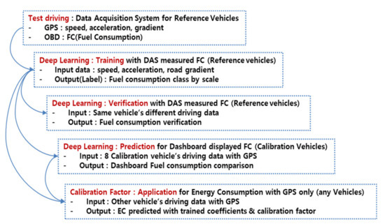
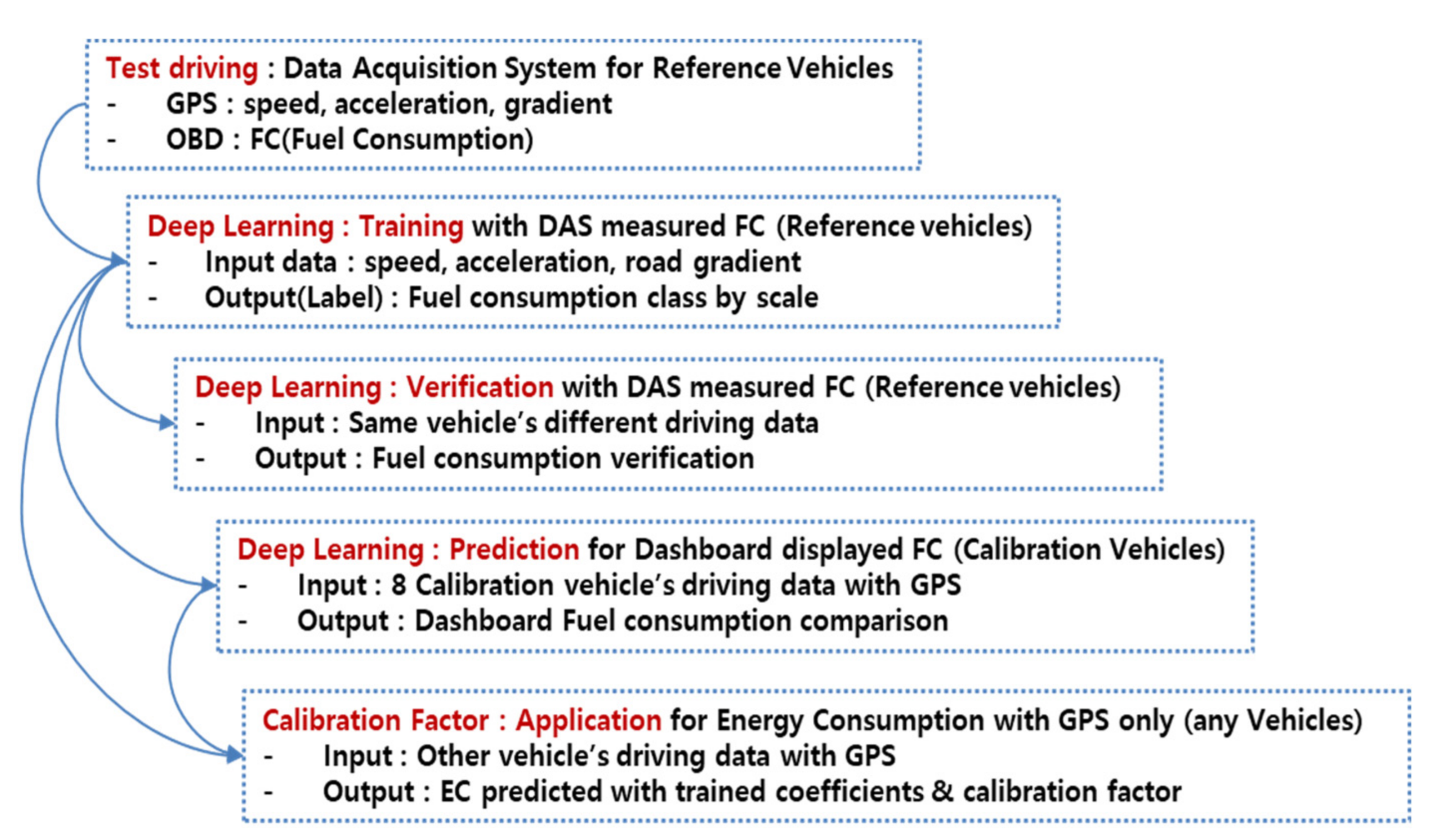
Figure 1 shows the process in brief. It is composed of ‘Test driving—D/L training (Labeled FC)—D/L verifying (Labeled FC)—D/L predicting (Average FE)—Calibrating (Average FE)’ processes. It proposes a proper calibrating scheme for internal combustion engine cars and a similar predicting way for a battery-powered electric car in the study. You cannot show the vehicle dynamics as precisely as the mechanical methods do with this technique but it is useful enough to hit the averaged FE values by training for the FC labels of the reference car with D/L and a simple calibration factor of test vehicles.

Figure 1. The proposed process of energy consumption monitoring of vehicles by deep learning.

2. Related Works

Let us look into the FC (Fuel Consumption) estimation methods proposed in previous works of other researchers. There are two categories in these fields. The first one is the mechanical or physics-based method using the driving resistance forces [11,12,13]. The force consists of four resistance terms. They are the friction, aerodynamic, gradient and inertia resistance force. You can calculate the necessary engine power by multiplying vehicle speed to the total resistance force. The fuel should be burned/consumed in the combustion chamber of the engine to keep the power transferring through the powertrain gears and axles then finally to the tire. The estimating process can be described in brief as follows:

R_friction = μWg

R_aerodynamic = 0.5 C_DρAv²

R_gradient = Wgsinθ

R_inertia = Wa

R_total = R_friction + R_aerodynamic + R_gradient + R_inertia

P = η R_total v

$$FC=\left\{\begin{array}{c}\xi P for Normal driving\\ F{C}_{idle} for Idling state \\ 0 for Fuel-cut state\end{array}\right.$$

where,

• μ: Tire-road surface rolling friction coefficient;
• W: Vehicle weight [kg];
• g: Gravitational acceleration [=9.8 m/s²];
• C_D: Drag coefficient;
• ρ: Air density [kg/m³];
• A: Vehicle frontal area [m²];
• v: Vehicle speed [m/s];
• θ: Road gradient [degree];
• a: Vehicle acceleration [m/s²];
• η: Power transfer efficiency;
• ξ: Fuel-power conversion factor [mcc/Watt/s];
• R: Resistance force [N];
• P: Engine power [Watt];
• FC: Fuel consumption [mcc/s];
• FC_idle: Fuel consumption in idle state [mcc/s].

As you can see, it is rather complicated and there are many coefficients which are different for the types of vehicle/fuel and road conditions. However, it is accurate because it can capture the vehicle dynamics once you have all the coefficients available—but it is hard to obtain those coefficients because they are the internal/valuable numbers of the car manufacturers. The more harsh and interesting part is that the final FC value falls into a sector of three divisions (normal, idling, fuel-cut). If the vehicle drives normally, then the FC is proportional to the necessary engine power. However, fuel injection stops when the fuel-cut is activated. The fuel-cut is a basic function adopted in most modern vehicles [14,15]. It is live when the gas pedal is released with the gear engaged in drive position and engine speed kept higher than about 1200 rpm. It is for the better fuel economy using the inertial driving force. It is like the braking regeneration function for electric cars, including the hybrid ones. The last sector for FC is the idling state. It consumes fuel even in the short waiting period like stand-by in front of the traffic sign.

The FC estimation is a kind of classification problem with three sectors of normal, idling and fuel-cut driving state. The FC changes suddenly also for several driving events of wide open throttling, warming up the coolant after cold start, driving in high altitude area of low atmosphere pressure, lean-burn conditions of the part load driving, or handling for feedback signal from O₂ sensor in the exhaust pipe even in the normal driving state. The fuel-power conversion factor (ξ) for the normal driving FC calculation is not a constant value but it changes in sharp for different driving conditions. The fuel injection rate changes rapidly in the instant of entering each domain of driving conditions as mentioned just above. Therefore, FC estimation is a classification problem again for the injection controls dealing with all the changing conditions i.e., domains of injection. The deep-learning method is proper for the purpose. It is useful not only for the regression problems (the target answer varies in continue) but also for the classification ones (the target answer varies in several groups). Once you have secured the labeled dataset for the systems of concern, then it is easy to train the deep-learning parameters hitting the target labels with high precision. It is proposed in this study and you can see an FC labeling and classifying scheme of deep learning in the next sections.

The second method for FC estimation involves machine learning approaches [10,16,17]. These train parameters calculating FC with various input data. The input data is the states/conditions of vehicle and road usually. There are two types of machine learning methods for these approaches. The first one is a machine learning for average fuel economy with vehicle/road data [10,16]. The average fuel economy is in the unit of liter/km or km/100 liter and it is averaged over a fixed/variable time period or driven distance (like 1–5 km in [10]). The input data are averaged over the same period/distance. Then it trains the parameters estimating FE (Fuel economy) like a regression problem solving as follows:

Input = Average (state/conditions of vehicle/road)

Hidden = AF₁ (Input × W₁ + B₁)

Output = AF₂ (Hidden × W₂ + B₂)

$$Loss=MSE(FE,\mathit{Output})=\frac{1}{N}\sum {\left(F{E}_i-Outpu{t}_i\right)}^2$$

$$W_{\mathit{next}}=W_{\mathit{previous}}+\eta \times \frac{\partial Loss}{\partial W}$$

$$B_{\mathit{next}}=B_{\mathit{previous}}+\eta \times \frac{\partial Loss}{\partial B}$$

where,

• AF: Activation function (Usually sigmoid or Relu function);
• W: Weights parameters;
• B: Bias parameters;
• FE: Fuel Economy [km/liter] or [liter/100 km];
• MSE: Mean Square Error.

Usually, the number of neurons for input/hidden is about 5–10 and there is only one output neuron, i.e., the estimated average fuel economy value for the specific period/distance. The number of hidden layers is also just one in most previous works because layers should be simple for the single output value. All the characteristics make this kind of method a regression problem approach and 3-layer construction of machine learning (i.e., Input-Hidden-Output) with small numbers of neurons (for example, 12-5-1 in [10]). In short, the previous machine learning methods are a type of regressive solving for moving average of FC for the period/distance. These methods use general sates/conditions of vehicle/road as input data like speed, acceleration, curb weight, number of stops, duration of stops and some manipulated values of the previous data, i.e., speed squared, speed tripled, acceleration squared, etc., averaged over the specific period/distance. That is natural because it is difficult to get the coefficients of the vehicles and roads necessary to calculate the resistance forces as mentioned above for the mechanical FC estimation methods. The drawback of these previous machine learning techniques is that they cannot capture the vehicle dynamics without these coefficients and with the simple layers and small number of neurons. It is not enough to catch up the complex domain change of injection with these simple constructions. It thus makes them a method for solving averaged FE values in a regressive way. Therefore, you need an FC estimation method in real-time for more precise and practical vehicle FC monitoring capability, as proposed in the previous section.

The second and last approach of the machine learning category is guessing the certified fuel economy with vehicle technical data [17]. The input data are composed of engine size, engine cylinder numbers, engine valve numbers, fuel type, engine intake type, powertrain type, etc. These input flows into the hidden layer just like the one for the average fuel economy explained before. The construction is the same 3-layer (Input-Hidden-Output) and the output is just one value of certified fuel economy that is easy to obtain from a public database. There are three CFE data groups usually. They are for city, highway and mixed driving cycles in the standard test procedure. The numbers of neurons are about 22-10-3 in [17]. The three output neurons are for the city, highway and mixed driving CFE. In short, these methods cannot estimate even the average FE in real road driving. They just guess the fixed values of CFE with various vehicle characteristics. It makes these approaches useless for the vehicle energy consumption monitoring purpose.

You need a FC estimating method for the driving vehicles on the real road in real-time as proposed in the previous section. The proposed method estimates the average FE of any type of cars with trained parameters hitting the FC labels of the reference cars with the help of the calibrating factor that is simple and easy to obtain.

3. Materials and Methods

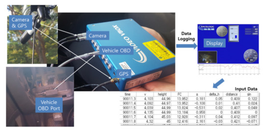
The ten test vehicles were driven on the road to measure the necessary data. The data are vehicle speed, acceleration rate, fuel consumption and road gradient obtained with a DAS named VBOX which is a well-known data logger for motor sports practice and it is manufactured by Racelogics Co. in Buckingham of UK. It is equipped with a GPS sensor and OBD connectors. Table 1 summarizes the specification of VBOX and Figure 2 shows VBOX connected to a test vehicle. The vehicle speed, acceleration rate and road gradient are measured by the GPS sensor and fuel consumption by OBD connection of VBOX. The data sampling resolution is 10 Hz.

Table 1. Specifications of DAS (VBOX).

Spec.	Accuracy	Resolution
Heading	0.1	0.01
Position	3.0 m	0.1 m
Distance	0.05%	1.0 cm
Speed	0.1 km/h	0.01 km/h
Acceleration	1.0%	0.01 G

Figure 2. DAS (VBOX) connected to a test vehicle.

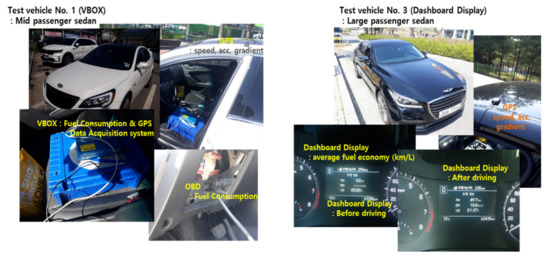
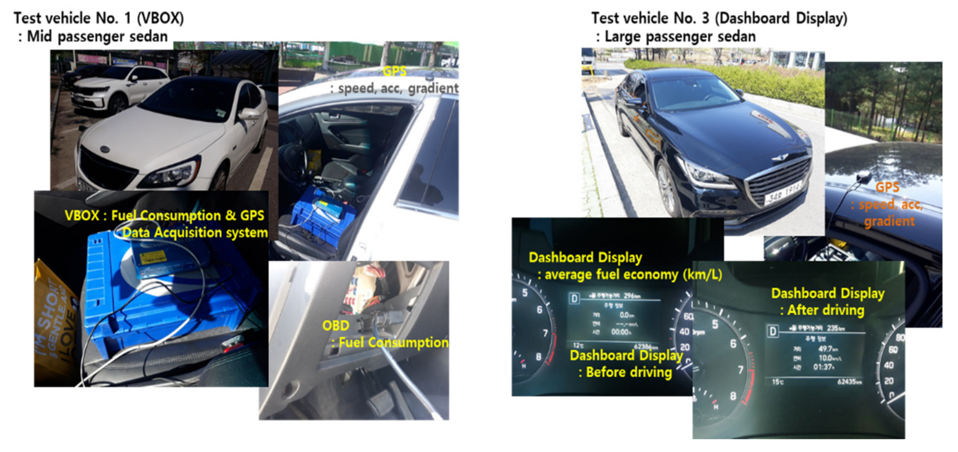
Table 2 shows the ten test vehicles specifications. The vehicle types of the test cars are passenger sedan, SUV, van and sub-compact. The model year ranges from 2010 to 2020 and the vehicle weight from 1200 kg to 2700 kg. Test vehicles No. 1 and No. 2 are the two reference cars fueled by gasoline and diesel, respectively. They were driven two times. The first driving data were used to train the parameters estimating fuel consumption by D/L technique and the second data to verify them. The other eight vehicles were driven to obtain fuel economy values displayed on the dashboard. These data are for the calibrating process of the parameters trained before. Test vehicle No. 10 is an electric car. The certified fuel (electricity) economy of No. 10 is 5.3 km/kWh, and it uses electricity economy in a precise unit. Figure 3 shows two test vehicles with VBOX and dashboard display as examples. The GPS sensor is fixed on the car roof and OBD connecter is signaled from the car OBD port under the driver’s dashboard as you can see in Figure 3. The signals are saved in the memory of VBOX then you can move the data to any PC to check and manipulate them.

Table 2. The specifications of test vehicles.

No.	Model Type	CFE 2 (km/L)	MY 3 (YYYY)	Weight 4 (kg)	Engine (cc)	Fuel	DAS Type	Test Times
1	Mid PS 1	11.0	2010	1875	2656	Gasoline	VBOX	2
2	Mid SUV	15.0	2012	2255	1995	Diesel	VBOX	2
3	Large PS	14.2	2014	2170	2143	Diesel	Dashboard	1
4	Large Van	9.5	2015	2980	2497	Diesel	Dashboard	1
5	Mid SUV	14.1	2019	2005	1995	Diesel	Dashboard	1
6	Small PS	13.7	2017	1575	1591	Gasoline	Dashboard	1
7	Sub Compact	15.2	2016	1280	998	Gasoline	Dashboard	1
8	Mid SUV	11.4	2016	2720	1998	Diesel	Dashboard	1
9	Mid Van	11.3	2020	2760	2199	Diesel	Dashboard	1
10	Mid SUV	5.3 5	2019	2080	EV 6	Electric	Dashboard	1

¹ PS: Passenger Sedan; ² CFE: Certified Fuel Economy; ³ MY: Model Year; ⁴ Weight: Gross total weight; ⁵ 5.3 km/kWh (Electricity Economy); ⁶ EV: Electric Vehicle.

Figure 3. Test vehicle No. 1 connected to VBOX and No. 3 showing the dashboard display of fuel economy as examples.

4. Results

4.1. Driving Test Results

Table 3 shows the measured fuel economy and driving data of the ten test vehicles. Test vehicles No. 1 and No. 2 are for reference data, measured by VBOX. These reference data are for training and verifying the parameters by a deep-learning procedure.

Table 3. Fuel economy measured for ten test vehicles with VBOX and dashboard display.

No.	Model Type	FE (km/L)	Test Purpose	DAS Type	Driving Distance (km)	Average Speed (km/h)
1	Mid PS	12.5	Training	VBOX	81.3	40.6
		7.7	Verifying	VBOX	9.7	17.0
2	Mid SUV	15.6	Training	VBOX	80.6	39.8
		12.8	Verifying	VBOX	12.5	20.6
3	Large PS	14.7	CAL. 1	Dashboard	28.5	21.5
4	Large Van	12.6	CAL.	Dashboard	79.6	63.8
5	Mid SUV	21.2	CAL.	Dashboard	71.6	53.0
6	Small PS	14.4	CAL.	Dashboard	27.4	20.3
7	Sub Compact	20.6	CAL.	Dashboard	48.2	38.0
8	Mid SUV	13.7	CAL.	Dashboard	63.8	49.0
9	Mid Van	15.7	CAL.	Dashboard	67.2	55.2
10	Mid SUV	9.3 2	CAL.	Dashboard	63.3	51.9

¹ CAL.: Calibration purpose; ² 9.3 km/kWh: Electricity Economy.

The training data of test vehicles No. 1 and No. 2 were gathered driving about 80 km, and the verifying data were for about 10 km driving. The data number is about 72,000 for training and about 7000 for verifying. The average speed is about 40 km/h for training and 20 km/h for verifying. The difference between the number and range of data for train/verification is very big. This is because you need a wide range of input data (speed/acceleration/gradient) and output data (fuel consumption) to train properly with a deep-learning technique [18]. However, lots of data are not necessary for verifying because it is just an accuracy check process [19]. The ratio of data number for training and verification is about 10 and this is reasonable for the D/L procedure.

Test vehicles No. 3 to No. 10 are for the calibration procedure. The input data (speed/acceleration/gradient) are measured by a GPS sensor and the output data (fuel economy) is the dashboard displayed average fuel economy values. The dashboard FE (Fuel Economy) is estimated with the fuel consumption and driven distance measured by ECU (Engine Control Unit) built in the vehicle [20]. The dashboard FE is not measured/recorded in real-time but it is rather a one-time value. You can record the value by resetting the FE display in the dashboard before starting to drive. It continues to change while driving and the final FE value is the last number shown in the dashboard just in the moment of ending of test drive. You cannot compare or analyze the FE every second like the VBOX-measured FC (Fuel Consumption), but the dashboard FE value can be used to calibrate the parameters trained by D/L with the reference test data. It is easy to get the dashboard FE data of various cars, but it is hard to connect VBOX to the OBD port and to set VBOX to extract the FC data. It is very difficult to get the FC data for cars whose OBD signal protocol is not open [21]. That is why there are just two reference vehicles with VBOX-measured FC data and eight test cars with dashboard-displayed FE data. The proposed monitoring method takes the detail fuel consumption data for training/verifying and it is calibrated with the rough FE data without the measuring difficulty of the OBD port and protocol problem.

4.2. D/L Results

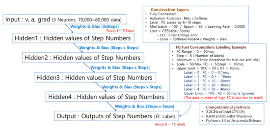
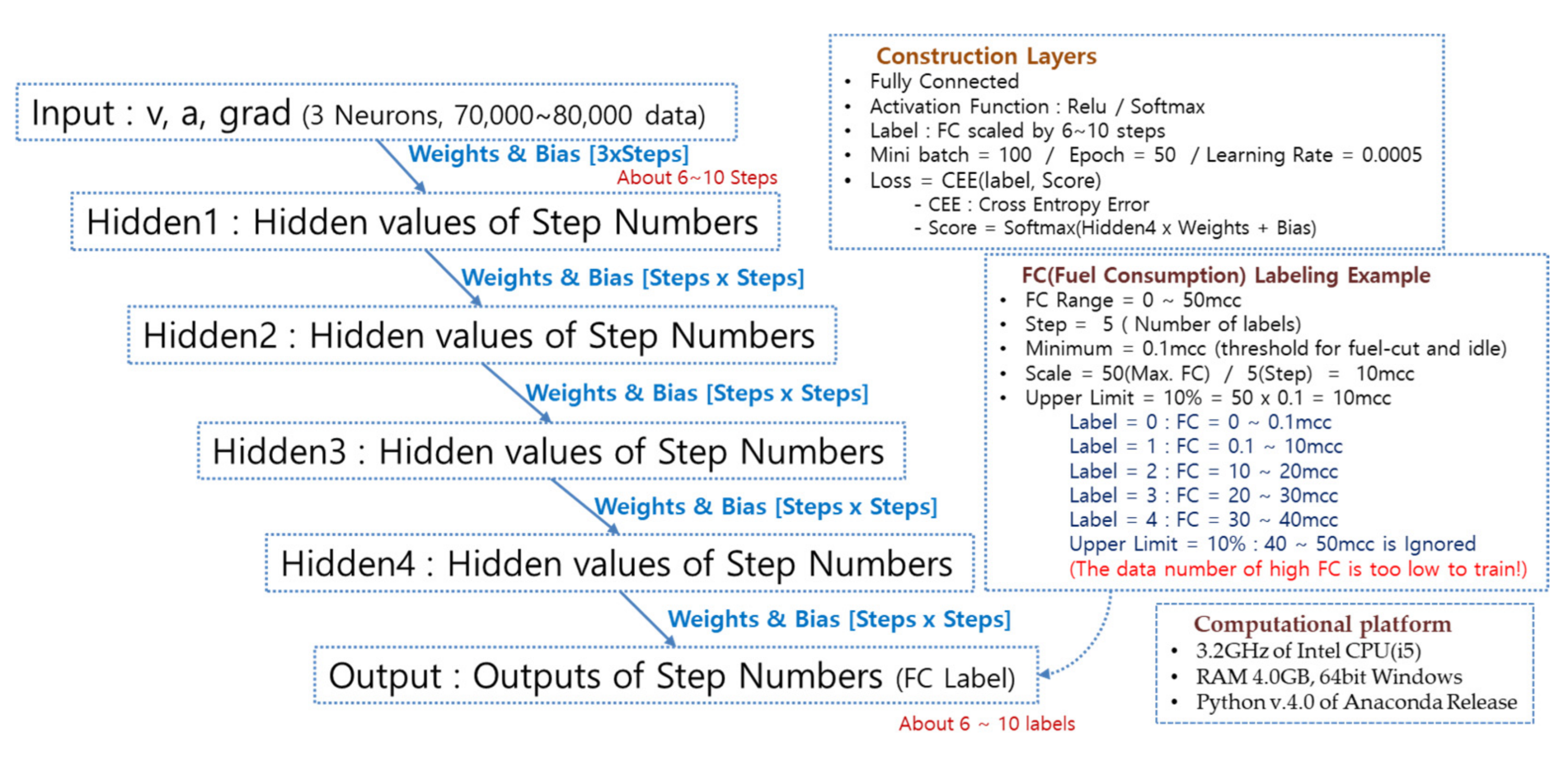
The VBOX-measured data of the reference vehicles are for training the parameters by D/L technique. The input data is speed/acceleration/gradient and output data is fuel consumption. Figure 4 shows the D/L layers construction to train the parameters (weights and bias) estimating FC with input data. There are four hidden layers and it makes the 5-layer D/L construction [22]. The output or label is the FC data. FC is divided by a scale factor to make the labels. The number of labels is about 6–8 in the D/L construction. The computational platform is 3.2 GHz of Intel CPU (i5), RAM 4.0 GB, 64 bit Windows and Python v.4.0 of Anaconda Release.

Figure 4. Deep-learning layers construction and the hyper-parameters.

The FC does not change continuously but steps up and down as the fuel injection domain like fuel-cut/idling/acceleration/warm-up changes while driving [23]. It makes the D/L procedure of estimating FC to be a classification problem not a regression one [24]. Therefore, you need a proper labeling scheme to train the parameters estimating FC values.

The labeling process is a little complicated, but it is presented in Figure 4 explaining a 5-label example. In the example, the maximum FC value is 50 mcc and the number of labels (steps) is 5, then the scale factor becomes 10 mcc/step (=50 mcc/5 steps). The label is scaled by 10 mcc in FC like, 10–20 mcc/20–30 mcc/… etc. Therefore, label 0 is for 0.0–0.1 mcc, label 1 is for 0.1–10 mcc, and label 2 is for 10–20 mcc of FC in the example. The 0.1 mcc is the threshold for fuel-cut and idle for label 0. The fuel is not injected during the fuel-cut period activated by releasing the gas pedal with gear in the drive position for better fuel efficiency. The FC for idle is about 2–3 mcc for usual passenger cars [25]. Therefore, the FC is zero for fuel-cut then it steps up to idle FC value. There is no continuous FC value increasing from fuel-cut to idle state. The label 0 is for fuel-cut condition under the threshold of 0.1 mcc considering small fluctuation in the FC data.

In the FC labeling example of Figure 4, you can see the ‘Upper Limit’ term. It takes account of the fact that high FC around maximum value of 50 mcc is too small to train. It is exceptional to push the gas pedal to the wide open throttle while driving on the real road. The labels for FC data higher than the ‘Upper Limit’ are ignored so that the D/L construction train the parameters properly. The few FC data higher than the upper limit is included in the label of just below the upper limit. It makes FC data higher than the upper limit become the highest label 5 in the example, so that the D/L learns more reasonably [26]. The calculating procedure of each layer is as follows.

Hidden1 = Relu(Input × Weight1 + Bias1)

(1)

Hidden2 = Relu(Hidden1 × Weight2 + Bias2)

(2)

Hidden3 = Relu(Hidden2 × Weight3 + Bias3)

(3)

Hidden4 = Relu(Hidden3 × Weight4 + Bias4)

(4)

Output = Softmax(Hidden4 × Weight5 + Bias5)

(5)

Loss = CEE(Output, Label)

(6)

Meanwhile, Relu, Softmax and CEE are as follows.

Relu(x) = Maximum(0, x)

(7)

Softmax(x_i) = exp(x_i)/sum of exp(x_i)

(8)

CEE(x_i, y_i) = Cross Entropy Error (x_i, y_i) = Average of {−log_e(x_i × y_i)}

(9)

The value of ‘Loss’ in Equation (6) is minimized by the gradient descent method in the D/L process as follows.

W_i+1 = W − η × G_i

(10)

$$G_i=\frac{\partial Loss}{\partial W_i}$$

(11)

W is the weights or bias and G is the gradient of Loss per W in Equations (10) and (11). η in Equation (10) is the learning rate and the value is set to 0.0005 in the D/L construction. The weights and bias become the parameters estimating FC label with input data. The numbers of weights and bias are same as the step numbers. It makes the numbers of the estimating parameters to increase as the label number goes up. That is a flexible and reasonable way to be trained in the usual D/L process because you need more parameters to learn complex tasks having many labels [27]. The size of weights array of the second hidden layer is [5 × 5] for the example shown in Figure 4 because the step or label number is five.

The parameters are trained with the first data of the reference test result then they are verified with the second data of the same reference vehicle. The D/L process is done for two reference vehicles fueled by gasoline and diesel, respectively. The fuel consuming mechanism is little different for gasoline and diesel [28]. That is why the reference vehicle should be assigned to different fuel type. The parameters of the gasoline car are calibrated with the FE of gasoline cars and the parameters of the diesel one is done with the diesel car’s FE result in next phase. Table 4 shows the training and verifying results of D/L for the two reference vehicles.

Table 4. The results of D/L trained and verified fuel economy for reference vehicles.

No.	Fuel (Car Type)	D/L Purpose	VBOX Measured FE (km/L)	D/L Estimated FE (km/L)	FC Steps	FC Upper Limit
1	Gasoline (Mid PS)	Training	12.5	12.5	6	35%
		Verifying	7.7	7.9
2	Diesel (Mid SUV)	Training	15.6	15.7	8	35%
		Verifying	12.8	12.7

The number of FC steps or labels is six for the gasoline car and eight for the diesel reference car in Table 4. It is determined by trial and error in the process of D/L training. The upper limit considering few data around maximum FC is 35% for both reference cars. The limit is chosen by trial and error also. The result of D/L training and verifying is good. For example, the VBOX-measured FE of the gasoline reference car is 12.5 km/L and trained parameters estimated it as 12.5 km/L, which is the exact same value. The verified FE is 7.9 km/L for 7.7 km/L of the VBOX-measured FE. The trained result for the diesel reference car is 15.7 km/L for 15.6 km/L of the VBOX-measured FE. The verified FE is 12.7 km/L for 12.8 km/L measured with VBOX, as shown in Table 4.

Table 5 and Table 6 show the detail FC data distribution for labels of the gasoline and diesel reference cars. The data for label 0 (fuel-cut) and high label (high engine load) is few in contrast to that of FC data that belong to label 1 and 2, corresponding to the idling state and low load range of engine power, respectively. The data distribution of FC like this is natural in that the cars were driven on the real road during daytime. The car is idle at the traffic sign often and runs slow for congestion usually. It means that the training data is proper for FC in the real-world driving in the study [29].

Table 5. The detail results of D/L procedure for gasoline reference vehicle.

Label	FC Range (mcc)	FC Data Number	FC Data Percentage
0	~0.10	5723	7.9%
1	~6.03	28,740	39.9%
2	~11.96	17,062	23.7%
3	~17.89	10,346	14.3%
4	~23.82	6446	8.9%
5	~29.75 (higher)	3802	5.3%

Table 6. The detail results of D/L procedure for diesel reference vehicle.

Label	FC Range (mcc)	FC Data Number	FC Data Percentage
0	~0.10	4663	6.4%
1	~3.34	27,584	37.8%
2	~6.58	9542	13.1%
3	~9.82	8311	11.4%
4	~13.06	8944	12.3%
5	~16.31	5777	7.9%
6	~19.55	4778	6.5%
7	~22.79 (higher)	3392	4.6%

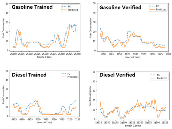
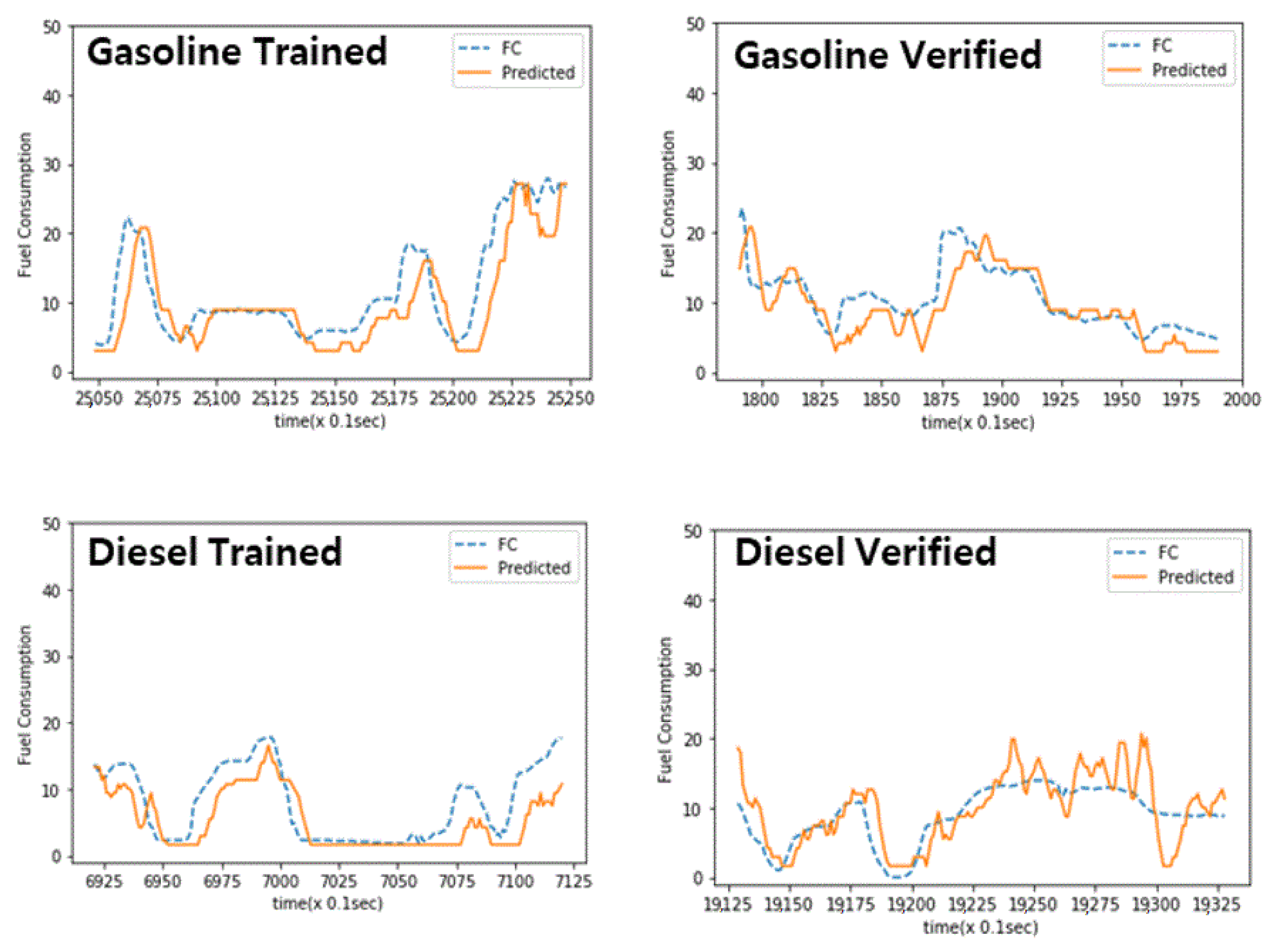
Figure 5 compares the D/L-estimated FC (in continuous line) with the VBOX-measured FC (in dotted line) during random time periods to get a sense of FC values. The close-up of the two FC data (Estimated vs. Measured) shows small differences in each value but the overall changing pattern is similar. The FE result of averaged FC for all the data is almost same as in Table 4 but the data cut from the random time period are slightly different as shown in Figure 5. The VBOX-measured FC moves more smoothly than the D/L-estimated FC in Figure 5. It is trained with GPS-measured speed/acceleration/gradient for the D/L estimation. The signals from the GPS are recorded by the resolution of 10 Hz, which is faster than the OBD signals of 1 Hz usually. The OBD signal of FC is just for inspection and maintenance practice [30]. It takes some time to burn the injected fuel. It means that ECU controls FC slowly because of the necessary time for the combustion process [31]. Therefore, the OBD signal of FC moves smoothly compared to the electronic signals from GPS sensors. It explains why D/L-estimated FC fluctuates more than the VBOX-measured FC in Figure 5.

Figure 5. D/L trained and verified FC estimated (continuous line) vs. FC measured (dotted line).

5. Discussion

The parameters were trained by D/L technique to estimate FC for the gasoline and diesel reference vehicles in the previous section. They estimate FE of the other eight test cars and Table 7 compares the measured FE by dashboard display and the predicted FE by the D/L trained parameters.

Table 7. Fuel economy compared: Dashboard display FE vs. D/L trained FE.

No.	Model Type	Dashboard Display FE (km/L)	D/L Estimated FE (km/L)	Reference Car	Ratio 1
3	Large PS	14.7	13.8	Diesel	1.065
4	Large Van	12.6	18.2	Diesel	0.692
5	Mid SUV	21.2	16.8	Diesel	1.262
6	Small PS	14.4	9.2	Gasoline	1.565
7	Sub Compact	20.6	12.5	Gasoline	1.648
8	Mid SUV	13.7	16.2	Diesel	0.846
9	Mid Van	15.7	15.8	Diesel	0.994
10	Mid SUV 2	9.3 2	12.8 15.5	Gasoline Diesel	0.727 0.600

¹ Ratio: FE_Dashboard / FE_D/L; ² Test No. 10 is for Battery Electric Vehicle [km/kWh].

The estimation is done for each fuel type. Test No. 6 and No. 7 are estimated by the gasoline reference parameters and Test No. 10 is predicted by both parameters because it is an electric car. The others are done by the diesel reference parameters. It seems that the D/L-estimated FE values do not match up with the measured FE ones. The ratios of the FE values in the last column of Table 7 are different for all the test vehicles. However, it is reasonable that the FE becomes bad as times goes by and FE keeps high for cars having good fuel efficiency. It implies that the parameters have to take account of some characteristics of each vehicle. The correction should be done by vehicle characteristics that are easily obtainable also for the monitoring practice. It is proposed a calibration factor considering CFE and MY as follows.

$$Calibration Factor=\frac{CF{E}_{test}}{CF{E}_{reference}} + \frac{\left(M{Y}_{test}-M{Y}_{reference}\right)}{30}$$

(12)

$$FE=F{E}_{DeepLearning}\times Calibration Factor$$

(13)

MY in Equation (12) is the number of the year written on the car registration paper like 2010, 2017, etc. MY for the gasoline reference cars (No. 1 and No. 6) are 2010 and 2017, respectively. CFE is 11.0 km/L for reference car No. 1 and 13.7 km/L for test car No. 6. Then, the calibration factor for No. 6 becomes as follows.

$$Calibration Factor=\frac{13.7}{11.0} +\frac{\left(2017-2010\right)}{30}=1.479$$

(14)

Table 8 shows the calibrated final FE values and errors from the dashboard-measured FE values. You can see the calibration factor of 1.479 for test vehicle No. 6 in Table 8. The calibration factor is multiplied by the D/L-estimated FE value. The final value of FE goes up with the calibration factor higher than 1.0 and it makes the error to be 5.5% for test vehicle No. 6 in Table 8. It seems to be a quite good prediction for FE. The results are rather similar for other test cars with this scheme of calibration of FE. The range of error is about −6.0 to +7.0%, which is reasonable to monitor any vehicle on the real road in real-time.

Table 8. Fuel economy calibrated with certified fuel economy and model year.

No.	Model Type	Dashboard Display FE (km/L)	Calibrated FE (km/L)	Error 1 (%)	Calibration Factor
3	Large PS	14.7	14.0	4.9	1.013
4	Large Van	12.6	13.3	−5.9	0.733
5	Mid SUV	21.2	19.7	7.0	1.173
6	Small PS	14.4	13.6	5.5	1.479
7	Sub Compact	20.6	19.8	4.0	1.582
8	Mid SUV	13.7	14.5	−5.6	0.893
9	Mid Van	15.7	16.1	−2.6	1.020
10	Mid SUV 2	9.3 2	10.0 9.1	−7.6 2.2	0.782 0.587

¹ Error = 100 × (FE_Dashboard − FE_Calibrated) / FE_Dashboard; ² Test No. 10 is for Battery Electric Vehicle [km/kWh].

The proposed calibration factor means that recent cars with good CFE would have high FE value for the same driving states/conditions like speed, acceleration and road gradient. You can get the data of CFE and MY from the registration paper of the vehicle, and the data for the vehicles used in this research were included in Table 2.

Test No. 10 is for the electric vehicle and the predicted result is more accurate when estimated by the diesel reference parameters. It may imply that the electric car spends energy in a similar pattern to the diesel car. It may be because that the test No. 10 electric vehicle is a mid-size SUV like the diesel reference car. However, the estimated result of the study right now is that the electric car’s energy consumption is estimated more precisely by the diesel reference parameters. It is necessary to test more EVs and we are preparing the test and estimation in future.

There are many factors acting on FE, except CFE and MY considered in the study. It is necessary to consider the other conditions like passenger/freight weight, wet/dry weather, on/off of auxiliary parts like air-conditioner, hot/cold air temperature, etc. However, considering CFE, it is measured on the chassis dynamometer driving standard cycles under the road load condition [32]. The term of ‘road load’ means driving resistance force of the car. It includes rolling friction resistance and aerodynamic resistance with curb weight condition. The effect of the tire–road friction, weight and car surface design is contained in the CFE in some degree. In other words, the most significant car characteristics are already included in the CFE. The MY reflects the aging effect of the car and it is a key factor for the change of the FE also.

The biggest effect of other car elements is the weight change due to the passenger numbers and freight load. FE changes with the various freight weight especially for large trucks and buses. You must take into consideration the weight change for these car categories and it is not reflected in the calibration process in this study. We are preparing the vehicle monitoring service system, and the dataset will be available to accommodate the other factors like weight, weather and auxiliary change in future. The calibration factor is a useful approach to monitor energy consumption with a small number of car characteristics. It may become a more and more reliable method as it includes other effects in addition to the CFE and MY already considered in this study.

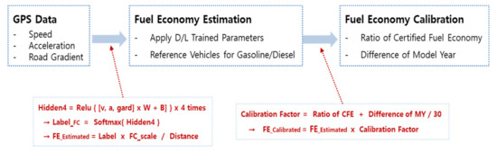
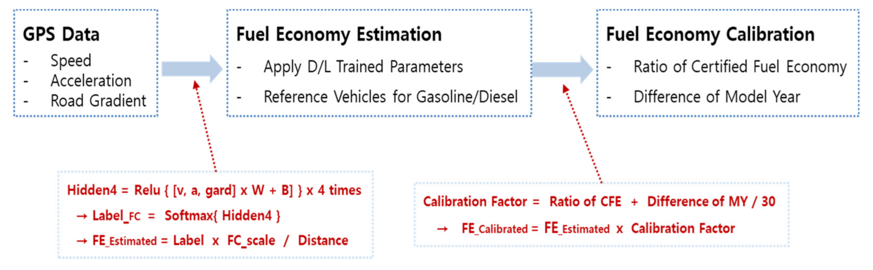
You can monitor energy consumption of vehicles with D/L-trained parameters of reference vehicles corrected with CFE and MY. Figure 6 shows the monitoring process proposed in the study once you have secured the D/L-trained parameters and the calibrated factors.

Figure 6. FC monitoring process with trained parameters and calibration factor.

6. Conclusions

It is useful to monitor the EC (energy consumption) of vehicles in real-time. It is proposed that the EC monitoring is possible with deep-learning technique. The fuel consumption of gasoline and diesel reference cars is measured by VBOX that is a well-known data logger equipped with a GPS sensor and OBD connector. The GPS sensor is used for vehicle speed, acceleration rate and road gradient, while the OBD connector is used for fuel consumption measurement.

The D/L technique is applied to optimize the parameters estimating FC with input data (speed/acceleration/gradient) for the reference cars. The FC data is scaled to make the labels in the D/L procedure. The FC does not change continuously but steps up and down as the fuel injection domain changes. It makes the D/L procedure of estimating FC to be a classification problem, not a regression one. The parameters are trained by the proposed 5-layer D/L construction with input data and output data for gasoline/diesel reference cars. The trained parameters estimated FC values for the verifying data precisely for the same reference cars respectively.

Then the parameters predicted FE of the other eight test vehicles, but the predicted FE values did not go well with the measured ones. That is natural for the wide range of fuel efficiency and deterioration degree of the test cars. Therefore, a calibration factor is suggested in the point of view that recently released cars having good fuel efficiency would keep the FE high. We thus suggest a calibration factor derived from certified fuel efficiency and model year, which you can easily obtain from the car registration paper.

It is possible to make an accurate estimation of FE by the parameters trained by the D/L technique and the calibration factor made from CFE and MY for the test cars. The error ranges from −6% to 7% for FE of the eight test cars. The necessary data to estimate FE is just vehicle speed, acceleration rate and road gradient, which are measurable with a GPS sensor without difficulty. You can get the final FE value with the trained parameters and the calibration factor.

It is easy to monitor energy consumption of vehicles by the proposed method on the real road in real-time with just a GPS sensor that is cheap and common. The FE estimating process is simple also because you can get the FE values by multiplying and adding the trained parameters four times then applying the calibration factor once for the test cars. The calculating process is so simple and easy that you can monitor the energy consuming pattern of any vehicles in real-time on the spot.

The same scheme was used for an electric vehicle and a more accurate result was obtained by the parameters of the diesel reference car. However, the result is just for one electric car, and more tests of battery-powered cars are needed in the future.

The other car characteristics such as weight, weather and auxiliary change were not included in the calibration factor and it will be added with monitoring service system that is being prepared. For example, cars decelerate by the vehicle weight, aerodynamic drag and tire rolling friction during the fuel-cut driving on the road. You can guess the weight/drag/friction change of the specific cars for the fuel-cut driving condition with the service system, and then the change can be reflected to estimate the FE properly.

References

- Todd, L. Changing North American vehicle-travel price sensitivities: Implications for transport and energy policy. Transp. Policy 2013, 28, 2–10. [Google Scholar] [CrossRef] [Scilit]
- Huang, W.; Guo, Y.; Xu, X. Evaluation of real-time vehicle energy consumption and related emissions in China: A case study of the Guangdong–Hong Kong–Macao greater Bay Area. J. Clean. Prod. 2020, 263, 121583. [Google Scholar] [CrossRef] [Scilit]
- Yao, Z.; Wang, Y.; Liu, B.; Zhao, B.; Jiang, Y. Fuel consumption and transportation emissions evaluation of mixed traffic flow with connected automated vehicles and human-driven vehicles on expressway. Energy 2021, 230, 120766. [Google Scholar] [CrossRef] [Scilit]
- Elvin, C.; Ng, Y.; Huang, Y.; Hong, G.; Zhou, J.L.; Surawski, N.C. Reducing vehicle fuel consumption and exhaust emissions from the application of a green-safety device under real driving. Sci. Total Environ. 2021, 793, 148602. [Google Scholar] [CrossRef] [Scilit]
- Zhang, Y.T.; Claudel, C.G.; Hu, M.B.; Yu, Y.H.; Shi, C.L. Develop of a fuel consumption model for hybrid vehicles. Energy Convers. Manag. 2020, 207, 112546. [Google Scholar] [CrossRef] [Scilit]
- Liu, J.; Khattak, A.; Wang, X. The role of alternative fuel vehicles: Using behavioral and sensor data to model hierarchies in travel. Transp. Res. Part C Emerg. Technol. 2015, 55, 379–392. [Google Scholar] [CrossRef] [Scilit]
- Tanaka, S. When tax incentives drive illicit behavior: The manipulation of fuel economy in the automobile industry. J. Environ. Econ. Manag. 2020, 104, 102367. [Google Scholar] [CrossRef] [Scilit]
- Malik, M.; Nandal, R. A framework on driving behavior and pattern using On-Board diagnostics (OBD-II) tool. Mater. Today Proc. 2021. [Google Scholar] [CrossRef] [Scilit]
- Baek, S.H.; Jang, J.W. Implementation of integrated OBD-II connector with external network. Inf. Syst. 2015, 50, 69–75. [Google Scholar] [CrossRef] [Scilit]
- Alexander, S.; Byerly, A.; Hendrix, B.; Bagwe, R.; Santos, E.; Ben-Miled, Z. A machine learning model for average fuel consumption in heavy vehicles. IEEE Trans. Veh. Technol. 2019, 1–10. [Google Scholar] [CrossRef] [Scilit]
- Lee, S.; Lee, B.; Zhang, H.; Sze, C. Development of greenhouse gas emissions model for 2014-2017 heavy- and medium-duty vehicle compliance. SAE Tech. Pap. 2011. [Google Scholar] [CrossRef] [Scilit]
- Fontaras, G.; Luz, R.; Anagnostopoulos, K.; Savvidis, D.; Hausberger, S.; Rexeis, M. Monitoring CO2 emissions from HDV in Europe—An experimental proof of concept of the proposed methodological approach. In Proceedings of the Conference on Transport and Air Pollution (TAP), Graz, Austria, 18–19 September 2014; Available online: https://publications.jrc.ec.europa.eu/repository/handle/JRC91415 (accessed on 8 June 2021).
- Ko, K.H.; Moon, B.K.; Lee, T.W. An economic calibration method for fuel consumption model in HDM4. Wirel. Pers. Commun. 2016, 89, 959–975. [Google Scholar] [CrossRef] [Scilit]
- Boopathi, R.; Gopinath, E. Performance analysis of plastic oil blend by changing the fuel injection timing in diesel engine. Mater. Today Proc. 2021, 46, 4613–4618. [Google Scholar] [CrossRef] [Scilit]
- Huang, Y.; Ng, E.C.Y.; Zhou, J.L.; Surawski, N.C.; Lu, X.; Du, B.; Forehead, H.; Perez, P.; Chan, E.F.C. Impact of drivers on real-driving fuel consumption and emissions performance. Sci. Total Environ. 2021, 798, 149297. [Google Scholar] [CrossRef] [Scilit] [PubMed]
- Wickramanayake, S.; Dilum, B.H.M.N. Fuel consumption prediction of fleet vehicles using machine learning: A comparative study. In In Proceedings of the Moratuwa Engineering Research Conference (MERCon 2016), Moratuwa, Sri Lanka, 5–6 April 2016; 90–95. [Google Scholar] [CrossRef] [Scilit]
- Ziółkowski, J.; Oszczypała, M.; Małachowski, J.; Szkutnik-Rogoż, J. Use of artificial neural networks to predict fuel consumption on the basis of technical parameters of vehicles. Energies 2021, 14, 2639. [Google Scholar] [CrossRef] [Scilit]
- Shang, M.; Zhou, Y.; Fujita, H. Deep reinforcement learning with reference system to handle constraints for energy-efficient train control. Inf. Sci. 2021, 570, 708–721. [Google Scholar] [CrossRef] [Scilit]
- Ghosh, R. A Recurrent Neural Network based deep learning model for offline signature verification and recognition system. Expert Syst. Appl. 2021, 168, 114249. [Google Scholar] [CrossRef] [Scilit]
- González, E.G.; Flórez, J.A.; Arab, S. Development of the management strategies of the ECU for an internal combustion engine: Computer simulation. Mech. Syst. Signal Process. 2008, 22, 1356–1373. [Google Scholar] [CrossRef] [Scilit]
- Vdovic, H.; Babic, J.; Podobnik, V. Eco-efficient driving pattern evaluation for sustainable road transport based on contextually enriched automotive data. J. Clean. Prod. 2021, 311, 127564. [Google Scholar] [CrossRef] [Scilit]
- Lee, K.; Silva, B.N.; Han, K. Algorithmic implementation of deep learning layer assignment in edge computing based smart city environment. Comput. Electr. Eng. 2021, 89, 106909. [Google Scholar] [CrossRef] [Scilit]
- Cavicchi, A.; Postrioti, L. Simultaneous needle lift and injection rate measurement for GDI fuel injectors by laser Doppler vibrometry and Zeuch method. Fuel 2021, 285, 119021. [Google Scholar] [CrossRef] [Scilit]
- Moradi, E.; Moreno, L.M. Vehicular fuel consumption estimation using real-world measures through cascaded machine learning modeling. Transp. Res. Part D Transp. Environ. 2020, 88, 102576. [Google Scholar] [CrossRef] [Scilit]
- Cui, Y.; Xu, H.; Zou, F.; Chen, Z.; Gong, K. Optimization based method to develop representative driving cycle for real-world fuel consumption estimation. Energy 2021, 235, 121434. [Google Scholar] [CrossRef] [Scilit]
- Sun, R.; Chen, Y.; Dubey, A.; Pugliese, P. Hybrid electric buses fuel consumption prediction based on real-world driving data. Transp. Res. Part D Transp. Environ. 2021, 91, 102637. [Google Scholar] [CrossRef] [Scilit]
- Langer, S. Analysis of the rate of convergence of fully connected deep neural network regression estimates with smooth activation function. J. Multivar. Anal. 2021, 182, 104695. [Google Scholar] [CrossRef] [Scilit]
- Chaudhari, V.D.; Deshmukh, D. Diesel and diesel-gasoline fuelled premixed low temperature combustion (LTC) engine mode for clean combustion. Fuel 2020, 266, 116982. [Google Scholar] [CrossRef] [Scilit]
- Kongjian, Q.; Minggao, O.; Qingchun, L.; Maodong, F.; Jidong, G.; Junhua, G. Development and validation of emissions and fuel economy test procedures for heavy duty hybrid electric vehicle. In Proceedings of the 2010 IEEE Vehicle Power and Propulsion Conference (VPPC 2010), Lille, France, 1– September 2010; 2010; pp. 1–5. [Google Scholar] [CrossRef] [Scilit]
- Yang, L.; Zhang, S.; Wu, Y.; Chen, Q.; Niu, T.; Huang, X.; Zhang, S.; Zhang, L.; Zhou, Y.; Hao, J. Evaluating real-world CO2 and NOX emissions for public transit buses using a remote wireless on-board diagnostic (OBD) approach. Environ. Pollut. 2016, 218, 453–462. [Google Scholar] [CrossRef] [Scilit]
- Carlos, J.M.; Ola, S.; Per, T. In-Cycle Closed-Loop Combustion Control with Pilot-Main Injections for Maximum Indicated Efficiency. IFAC Pap. 2018, 51, 92–98. [Google Scholar] [CrossRef] [Scilit]
- Li, G.; Chen, Y.; Cao, D.; Qu, X.; Cheng, B.; Li, K. Extraction of descriptive driving patterns from driving data using unsupervised algorithms. Mech. Syst. Signal Process. 2021, 156, 107589. [Google Scholar] [CrossRef] [Scilit]
Publisher’s Note: MDPI stays neutral with regard to jurisdictional claims in published maps and institutional affiliations. |
© 2021 by the authors. Licensee MDPI, Basel, Switzerland. This article is an open access article distributed under the terms and conditions of the Creative Commons Attribution (CC BY) license (https://creativecommons.org/licenses/by/4.0/).