Comparative Performance Evaluation of Six Federated Learning Frameworks Under Locked FedAvg: Native SDKs and a Shared Reference Harness for Edge-Oriented 6G Applications

Abstract

Federated learning (FL) enables privacy-preserving collaborative training at the network edge, a core capability envisioned for sixth-generation (6G) wireless systems. While surveys and scale-oriented benchmarks advance FL methodology, documented, head-to-head comparisons of mainstream Python frameworks under identical FedAvg settings remain scarce. We benchmark six frameworks—Flower, TensorFlow Federated (TFF), FedML, NVIDIA FLARE, OpenFL, and PySyft—distinguishing two native SDK integrations (Flower, TFF) from four runs of a shared PyTorch FedAvg reference harness (FedML, NVIDIA FLARE, OpenFL, PySyft) in a controlled two-phase study on a Proxmox virtualized testbed with containerized runners, formalize the FedAvg objective and communication-cost model, and position our contribution against prior surveys, scale benchmarks, and single-framework documentation. Each framework–dataset pair is repeated over five IID partitions (random seeds 42–46); we report round-10 mean ± standard deviation for accuracy, wall time, and simulated communication volume. Phase 1 (MNIST) confirms protocol fairness ($99.22\pm 0.07$–$99.29\pm 0.06$% accuracy) with moderate wall-time spread; Phase 2 (CIFAR-10) exposes stack-dependent accuracy gaps (TFF $71.16\pm 0.23$% vs. ≈68% for PyTorch runners). We report per-round accuracy and loss curves with variability bands, wall-time comparisons, and simulated parameter traffic for all six frameworks across nine figures. The experimental protocol, model topology, and hyperparameters are specified in full; per-round JSON metrics and global model checkpoints are published. The study provides a documented baseline for 6G edge framework selection and for follow-on network-constrained and security experiments.

1. Introduction

Sixth-generation (6G) wireless networks—standardized internationally as IMT-2030 [1] and studied in parallel by 3GPP Release 20 [2]—will connect massive numbers of intelligent edge devices—smartphones, vehicles, industrial sensors, and wearables—that produce data locally but benefit from collaborative model training without centralizing raw data [3,4]. Unlike cloud-centric machine learning, edge intelligence pushes inference and increasingly training toward the network periphery [5,6], where uplink bandwidth, latency, and device availability are constrained [7,8]. Federated learning (FL) addresses this setting by keeping private datasets ${\mathcal{D}}_k$ on client devices while a coordinator aggregates model updates according to a shared protocol such as FedAvg [9,10,11].

1.1. Motivation: Framework Selection at the 6G Edge

Deploying FL in 6G scenarios involves more than choosing an aggregation algorithm. Systems engineers must select a software framework that orchestrates client–server communication, local training loops, checkpointing, and (optionally) privacy or security extensions [12,13,14]. Candidate stacks include Flower [15], TensorFlow Federated (TFF) [16], FedML [12], NVIDIA FLARE [13], OpenFL [17], and PySyft [14]. Each targets a different ecosystem, yet all frameworks must implement the same training protocol: broadcast ${\mathbf{w}}^{\left(t\right)}$, train locally, upload updates, aggregate, and evaluate.

Framework documentation and tutorials rarely address a deployment question: when the model, optimizer, data partition, and number of rounds are fixed, to what extent do accuracy, wall-clock time, and communication volume vary across frameworks?This question matters for 6G service orchestration because edge training jobs must fit within finite scheduling windows and uplink budgets [18,19]. A framework that is correct in principle but slow or communication-heavy may be unsuitable for URLLC-style deadlines or mMTC-scale deployments even if its API is convenient.

1.2. Evaluation Dimensions

We evaluate frameworks along three axes that map directly to Equations (5) and (6) in Section 3:

• Model quality—global test accuracy ${\mathrm{Acc}}^{\left(t\right)}$ and cross-entropy loss after each of $T=10$ communication rounds;
• Computational efficiency—total wall-clock time $T_{\mathrm{wall}}$ on a documented Proxmox containerized testbed;
• Communication cost—simulated parameter traffic $C_{\mathrm{total}}$ for every runner (native and reference), computed from serialized weight tensors (Section 3); this is not socket-level traffic in standalone simulation.

We deliberately hold the FL algorithm constant (FedAvg, IID partition) so observed differences reflect runtime stacks, orchestration overhead, and numerical training paths rather than algorithmic diversity [20]. We further distinguish native framework integrations from a shared reference PyTorch FedAvg loop (Section 3); the four reference-labelled frameworks validate harness parity rather than distinct product SDKs.

1.3. Research Questions and Paper Organization

This paper addresses three research questions:

• RQ1: Under identical FedAvg settings and IID data, how do six FL frameworks compare in accuracy and wall time on MNIST?
• RQ2: When task difficulty increases (CIFAR-10 edge vision), do framework rankings hold or do stack-specific dynamics widen gaps?
• RQ3: What communication volume does FedAvg incur, establishing a baseline before 6G bandwidth constraints?

Our study follows a two-phase design: Phase 1 (MNIST) verifies protocol correctness quickly; Phase 2 (CIFAR-10) stresses the same frameworks on a harder vision task representative of camera and sensing workloads at the edge [5,21]. Section 2 reviews prior work; Section 2.5 positions our contribution against surveys, scale benchmarks, and vendor documentation. Section 3 formalizes FedAvg and describes the testbed. Section 4 presents accuracy, loss, timing, and communication results with nine figures. Section 5 and Section 6 interpret findings and outline 6G/security extensions.

2. Related Work

2.1. Federated Learning at the 6G Edge

Federated learning was introduced as a communication-efficient approach for training deep models on decentralized data [9,18]. Comprehensive surveys document algorithms, privacy mechanisms, and open problems [10,20,22]. For wireless and mobile networks, FL surveys emphasize latency, bandwidth, and heterogeneity constraints at the edge [7,11]. Sixth-generation network visions and FL-specific 6G surveys explicitly motivate distributed machine learning close to users and devices [1,2,3,4,19], while the edge-computing literature argues that intelligence should be pushed toward the network periphery [5,6,8]. Our work sits at this intersection: we do not yet model full 6G radio channels, but we establish documented framework baselines that future work can extend with bandwidth and latency profiles aligned to IMT-2030 usage scenarios [1].

Non-IID data, stragglers, and heterogeneous compute remain active research topics [23,24,25,26]. Security and privacy extensions—secure aggregation [27], differential privacy [28], and poisoning attacks [29,30]—are orthogonal to our Phase 1–2 ideal-network study but motivate the benchmark harness as a platform for later security chapters.

2.2. FL Frameworks and Tooling

Multiple open-source FL frameworks target different ecosystems. Flowerprovides a framework-agnostic client–server abstraction widely used in research [15]. TensorFlow Federated (TFF) integrates tightly with TensorFlow and supports simulation at scale [16]. FedML targets cross-device and cross-silo production workflows with a unified research library [12]. NVIDIA FLARE focuses on enterprise and regulated deployments, including clinical use cases [13]. OpenFL supports Intel-based federated research clusters [17]. PySyft emphasizes privacy-preserving and encrypted computation over distributed data [14,31].

Each project publishes tutorials and performance claims for its own runtime. However, framework documentation typically demonstrates a single stack under settings chosen by the vendor. Cross-framework comparisons are rarely conducted with matched models, optimizers, random seeds, and aggregation semantics. Because frameworks are not interoperable in one federated round, fair comparison requires a disciplined experimental protocol—the gap our study addresses.

2.3. FL Benchmarks and Empirical Studies

Several benchmark suites study federated learning at scale or in realistic domains. LEAF provides federated datasets and reference implementations for natural user partitions [32]. FedScale benchmarks system and model performance with thousands of clients, focusing on scalability and scheduling [33]. FLBench proposes a broader benchmark suite across tasks and algorithms [34]. FLamby targets healthcare cross-silo settings with domain-realistic datasets [35]. Centralized reproducibility efforts such as MLPerf train on fixed tasks with locked hyperparameters and multi-run reporting; although not federated, their emphasis on transparent protocols and variance reporting informs our experimental design [36]. These contributions advance FL methodology and scale but generally emphasize algorithms, datasets, or system scheduling rather than answering: given the same FedAvg job, how do today’s popular Python FL frameworks differ in accuracy, time, and bytes?

2.4. Framework Selection Beyond Accuracy

Practitioners also weigh maintainability, learning curve, community support, and compatibility with edge/6G infrastructure (Kubernetes orchestration, gRPC transports, hardware accelerators) when adopting an FL stack [12,13,17]. Our study does not score qualitative factors; instead, it supplies documented accuracy, timing, and communication baselines that can be combined with organisational constraints in deployment checklists. We position the work against recent cross-framework FL studies and scale benchmarks in Table 1; we moderate novelty claims to locked FedAvg metrics with explicit native-versus-reference labelling and public per-round artifacts for the six named stacks [37].

Table 1. Positioning of this paper relative to prior FL research.

Dimension	FL Surveys [7,10]	Scale Benchmarks [32,33]	Framework Docs [12,15]	This Paper
Primary goal	Taxonomy, open problems	Scalability, scheduling	Single-stack usage	Cross-framework performance
Frameworks compared	Many (conceptual)	1–2 per study	1 per document	6 (same protocol)
Algorithm fixed	No	Varies	N/A	FedAvg only
Model/data fixed	No	Per benchmark	Per tutorial	Same CNN, seed, split
Native vs ref. reporting	No	Partial	N/A	Explicit labelling
Protocol specification	Theory only	Partial	Informal	Section 3
6G/edge motivation	Yes	Partial	Rare	Central + future profiles
Documented methodology	N/A	Partial	Partial	Protocol + public results [37]
Two-phase difficulty	No	Per task	No	MNIST then CIFAR-10

Note: N/A, not applicable.

2.5. Research Gap and Added Value

Table 1 contrasts our study with representative prior lines of work. Existing resources are complementary; none simultaneously (i) compare six mainstream frameworks under locked hyperparameters and model topology, (ii) formalize the exact FedAvg and communication equations implemented, (iii) publish per-round benchmark metrics and global model checkpoints alongside a containerized evaluation protocol [37], and (iv) structure experiments as a two-phase MNIST→CIFAR-10 progression aimed at 6G edge vision workloads.

Added value. This paper makes four concrete contributions beyond prior surveys and benchmarks:

• Controlled multi-framework comparison. We execute Flower, TFF, FedML, NVIDIA FLARE, OpenFL, and PySyft under one protocol (six IID clients, ten rounds, $\eta =0.01$, $B=32$, five seeds 42–46), isolating runtime effects from algorithmic diversity.
• Evidence that task difficulty matters. MNIST shows near-identical accuracy (≤0.07 pp spread across framework means) but measurable wall-time spread; CIFAR-10 exposes a ≈3.2 pp gap between TFF and the reference-cluster mean. This supports the methodological claim that easy datasets alone are insufficient for framework selection in edge vision scenarios.
• Documented 6G-oriented testbed. Proxmox virtual machines, per-framework container images, and a unified evaluation harness with per-round metric logging provide a transparent experimental record; benchmark metrics and global checkpoints are published in [37].
• Foundation for thesis extensions. Communication baselines (≈761 MB MNIST, ≈268 MB CIFAR-10, tensor-nbyte accounting) and the documented evaluation pipeline provide a starting point for 6G network profiles (eMBB, URLLC, mMTC), non-IID Dirichlet partitions [23], and security experiments [27,29] without redesigning the study design.

We report head-to-head FedAvg metrics for six widely cited Python FL stacks with explicit native-versus-reference implementation labels, a formal communication-cost model, and publicly released result artifacts [37].

3. Materials and Methods

3.1. Problem Formulation

We consider a cross-device federated learning setting with K clients indexed by $k\in \{1,\dots ,K\}$ [9,10]. Client k holds a private dataset ${\mathcal{D}}_k={\left\{(x_i,y_i)\right\}}_{i=1}^{n_k}$ drawn from an unknown distribution over the input–label space $\mathcal{X}\times \mathcal{Y}$. Let $N={\sum }_{k=1}^K{n}_k$ denote the total number of training samples. Each client trains a model parameterized by $\mathbf{w}\in {\mathbb{R}}^d$, where d is the number of learnable parameters.

The local empirical risk at client k is

$$F_k\left(\mathbf{w}\right)={\displaystyle \frac{1}{n_k}}\sum _{(x,y)\in {\mathcal{D}}_k}\ell \left(f_{\mathbf{w}}\left(x\right),y\right),$$

(1)

where $f_{\mathbf{w}}:\mathcal{X}\to {\mathbb{R}}^{\left|\mathcal{Y}\right|}$ is the neural network mapping, $\ell (·,·)$ is the cross-entropy loss, and $\left|\mathcal{Y}\right|=10$ for both MNIST and CIFAR-10. The global federated objective is the sample-size-weighted average

$$F\left(\mathbf{w}\right)={\displaystyle \sum _{k=1}^K}{\displaystyle \frac{n_k}{N}}{F}_k\left(\mathbf{w}\right).$$

(2)

In the ideal case, FL seeks ${\mathbf{w}}^{★}\in arg{min}_{\mathbf{w}}F\left(\mathbf{w}\right)$ without exchanging raw data ${\mathcal{D}}_k$ [11].

Table 2 summarizes the notations used throughout this paper.

Table 2. Mathematical notation.

Symbol	Description
K	Number of federated clients ($K=6$ in experiments)
${\mathcal{D}}_k$, $n_k$	Local dataset and its cardinality at client k
N	Total training samples, $N={\sum }_k{n}_k$
$\mathbf{w}\in {\mathbb{R}}^d$	Global model parameters
${\mathbf{w}}_k^{\left(t\right)}$	Client k model after local training at round t
$t\in \{0,\dots ,T-1\}$	Communication round index ($T=10$)
$\eta$	Learning rate ($\eta =0.01$)
E	Local epochs per round ($E=1$)
B	Mini-batch size ($B=32$)
$\ell (·,·)$	Cross-entropy loss function
$f_{\mathbf{w}}(·)$	CNN classifier
${\mathrm{Acc}}^{\left(t\right)}$	Global test accuracy after round t
$C_{\mathrm{round}}$	Communication bytes per federated round

3.2. Federated Averaging (FedAvg)

We employ Federated Averaging (FedAvg) [9], the de facto baseline algorithm for cross-framework comparison [18,20]. At communication round t, the server broadcasts the current global model ${\mathbf{w}}^{\left(t\right)}$ to all participating clients. Each client k performs E epochs of mini-batch stochastic gradient descent (SGD) on ${\mathcal{D}}_k$, initialized at ${\mathbf{w}}^{\left(t\right)}$. Denoting the local optimizer update by $\mathrm{LocalUpdate}(·)$, the client model after local training is

$${\mathbf{w}}_k^{(t+1)}=\mathrm{LocalUpdate}\left({\mathbf{w}}^{\left(t\right)};{\mathcal{D}}_k,\eta ,E,B\right).$$

(3)

The server aggregates client models by sample-size-weighted averaging:

$${\mathbf{w}}^{(t+1)}={\displaystyle \sum _{k=1}^K}{\displaystyle \frac{n_k}{N}}{\mathbf{w}}_k^{(t+1)}.$$

(4)

Equations (3) and (4) implement one local epoch of mini-batch SGD per client per round, followed by sample-size-weighted averaging [26]. All six frameworks in this study implement Equation (4); differences arise from runtime stacks (TensorFlow vs. PyTorch) and orchestration overhead, not from the aggregation formula itself.

For non-IID data, convergence of FedAvg can degrade because local objectives $F_k$ diverge from the global objective F [23]. Our experiments use IID partitions (uniform random split with fixed seed) to isolate framework effects; extensions to Dirichlet non-IID splits are planned [24,25].

3.3. Evaluation Metrics

After each round t, the global model ${\mathbf{w}}^{\left(t\right)}$ is evaluated on a held-out test set ${\mathcal{D}}_{\mathrm{test}}$:

$${\mathrm{Acc}}^{\left(t\right)}={\displaystyle \frac{1}{|{\mathcal{D}}_{\mathrm{test}}|}}\sum _{(x,y)\in {\mathcal{D}}_{\mathrm{test}}}\mathbb{I}\left[arg\underset{c}{max}{f}_{{\mathbf{w}}^{\left(t\right)}}{\left(x\right)}_c=y\right],$$

(5)

where $\mathbb{I}[·]$ is the indicator function and $f_{{\mathbf{w}}^{\left(t\right)}}{\left(x\right)}_c$ is the logit for class c. We also report the average cross-entropy loss on ${\mathcal{D}}_{\mathrm{test}}$. System-level metrics include total wall-clock time $T_{\mathrm{wall}}$ and per-round communication volume. For the reference PyTorch 2.13.0 runner, the simulated bytes per round are

$$C_{\mathrm{round}}={\displaystyle \sum _{k=1}^K}\left({\left|\mathbf{w}\right|}_{\mathrm{bytes}}+{\left|\mathbf{w}\right|}_{\mathrm{bytes}}\right)=2K{\left|\mathbf{w}\right|}_{\mathrm{bytes}},$$

(6)

where ${\left|\mathbf{w}\right|}_{\mathrm{bytes}}$ is the serialized model size (upload of client weights plus download of the global model). Over T rounds, $C_{\mathrm{total}}=T·C_{\mathrm{round}}$. Native Flower and TFF runners log the same tensor-nbyte accounting after each round (Section 3).

3.4. Two-Phase Experimental Design

We evaluate frameworks in two phases of increasing difficulty while holding FL hyperparameters constant (Table 3).

Table 3. Fixed hyperparameters for both experimental phases.

Parameter	Value
Clients	6
Communication rounds	10
Local epochs per round	1
Batch size	32
Learning rate	0.01
Optimizer	SGD (momentum 0.9, weight decay 0)
Local update	1 epoch of mini-batch SGD per round ($B=32$, shuffle with seed-specific generator)
Client participation	100% (all six clients each round)
Data partition	IID (uniform random split)
Random seeds	42, 43, 44, 45, 46 (five independent IID partitions)
Aggregation	FedAvg (sample-size-weighted)
Network profile	Ideal (0 ms latency, unlimited bandwidth)

Phase 1 uses MNIST [38] (28 × 28 grayscale digits) for fast framework screening. Phase 2 uses CIFAR-10 [21] (32 × 32 RGB images) as a closer proxy for edge vision workloads [5,39].

3.5. Models

Each dataset uses a lightweight convolutional neural network sized for edge feasibility [39]. Table 4 lists layer dimensions; full PyTorch 2.13.0 definitions appear in Appendix A. All activations are ReLU except the final linear layer (logits).

Table 4. CNN architectures and parameter counts (d).

Dataset	Layers (PyTorch)	d	${\left|\mathit{w}\right|}_{\mathbf{bytes}}$ (Float32)
MNIST	Conv($1\to 32$, $5\times 5$, pad 2), MaxPool; Conv($32\to 64$, $5\times 5$, pad 2), MaxPool; FC $3136\to 512$; FC $512\to 10$	1,662,858	6.65
CIFAR-10	Three Conv($3\to 32/64/64$, $3\times 3$, pad 1) blocks with MaxPool; FC $1024\to 512$; FC $512\to 10$	586,250	2.35

TFF implements an equivalent Keras model (same tensor shapes); Flower and the shared reference use the PyTorch modules in Appendix A. The parameter count d determines ${\left|\mathbf{w}\right|}_{\mathrm{bytes}}=4d$ in Equation (6) for PyTorch runners; native TFF uses the Keras weight tensors, yielding the same order of magnitude (∼761 MB and ∼268 MB total over ten rounds in our logs).

3.6. Framework Implementations

Table 5 lists the runner used per framework. Flower (v1.31.0) [15] and TFF (v0.85.0) [16] use native integrations. FedML [12], NVFlare [13], OpenFL [17], and PySyft [14] execute a shared PyTorch 2.13.0 FedAvg reference loop implementing Equations (3) and (4) with identical CNN, data split, and hyperparameters. Differences among the four reference-labelled rows therefore test harness stability, not separate SDK code paths.

Table 5. Framework runner fidelity.

Framework	Runner	Software Version
Flower	Native (Flower simulation)	1.31.0
TFF	Native (TensorFlow Federated)	0.85.0
FedML	PyTorch FedAvg reference	PyTorch 2.13.0
NVIDIA FLARE	PyTorch FedAvg reference	PyTorch 2.13.0
OpenFL	PyTorch FedAvg reference	PyTorch 2.13.0
PySyft	PyTorch FedAvg reference	PyTorch 2.13.0

Why native SDKs were not used for all six frameworks. Under our constraints (FedAvg only, six co-located simulated clients, pinned container images, no enterprise cluster), we could not obtain reproducible native FedAvg paths for FedML, NVFlare, OpenFL, and PySyft without diverging from the locked protocol (different aggregation hooks, optional privacy layers, or cluster-only entry points). Rather than compare incomparable tutorials, we (i) run Flower and TFF through their documented simulation APIs and (ii) use one audited PyTorch reference loop for the remaining stacks, explicitly labelled in every table and figure. Future work will replace reference rows with native SDK integrations where vendors expose FedAvg-compatible simulation modes.

Results are labelled as native (framework SDK) or reference (shared PyTorch loop) throughout tables and figures.

3.7. Benchmark Harness and Infrastructure

We developed a custom benchmark harness to enforce protocol parity across frameworks. The harness (i) loads MNIST and CIFAR-10 with a fixed IID partition per random seed, (ii) instantiates the dataset-specific CNN, (iii) orchestrates ten FedAvg rounds with the hyperparameters in Table 3, (iv) evaluates the global model on the held-out test set after each round, and (v) records accuracy, loss, wall time, and simulated communication volume for every runner. For frameworks without a native FedAvg path under our constraints, the same harness invokes a shared PyTorch reference loop so that local training, aggregation, and evaluation follow Equations (3)–(5) exactly.

Communication measurement. Standalone simulation does not emit physical network packets; instead, each round logs ${\left|\mathbf{w}\right|}_{\mathrm{bytes}}$ from serialized model tensors (NumPy nbytes for PyTorch state dicts; Keras weight arrays for TFF). Upload and download totals follow Equation (6). This definition matches across native and reference runners and should not be confused with gRPC/protobuf wire size in distributed deployments.

3.8. Statistical Protocol

Each framework–dataset combination is executed once per seed in $\{42, 43, 44, 45, 46\}$, yielding five independent IID partitions ($n=5$). We report the mean and sample standard deviation of round-10 test accuracy, final loss, total wall time $T_{\mathrm{wall}}$, and $C_{\mathrm{total}}$. Per-round curves plot the mean across seeds with shaded $\pm 1$ standard deviation bands. Operational outliers are defined a priori as runs whose wall time exceeds three times the median wall time of peer frameworks on the same dataset or that terminate with a container out-of-memory (exit code 137); such runs are excluded from aggregates and reported with the relevant results.

Experiments run on a Proxmox hypervisor (worker VM: 4 vCPUs, 8 GB RAM, Ubuntu 22.04.05 LTS) with two Ubuntu 22.04.05 LTS Server virtual machines [40]: a coordinator host (reserved for optional distributed aggregation; idle in the standalone configuration) and a worker host that executes one framework container at a time. The worker was allocated 4 vCPUs and 8 GB RAM. Each framework is packaged in an isolated container image with pinned SDK dependencies to avoid cross-contamination between runs.

For each framework $f\in \{\mathrm{flower},\mathrm{tff},\mathrm{fedml},\mathrm{nvflare},\mathrm{openfl},\mathrm{pysyft}\}$ and dataset $d\in \{\mathrm{MNIST},\text{CIFAR-10}\}$, the workflow comprises three steps: build the framework-specific container image, execute the federated benchmark on the worker host, and archive per-round metrics together with the final global model state. All runs use standalone simulation: six virtual clients co-located inside a single container, under an ideal network profile (zero latency, unlimited bandwidth). This isolates framework runtime and training-stack effects from distributed networking variability. Per-round JSON summaries and global model checkpoints are published in the public results repository [37]; benchmark source code and container images are not included there.

4. Results

This section reports empirical answers to RQ1–RQ3 from 60 benchmark runs (six frameworks × two datasets × five seeds). All figures use per-round metric logs; shaded bands or error bars denote $\pm 1$ standard deviation across seeds. Solid lines and hatched bars denote native runners (Flower, TFF); dashed lines denote the shared PyTorch reference loop (FedML, NVFlare, OpenFL, PySyft).

4.1. Overview

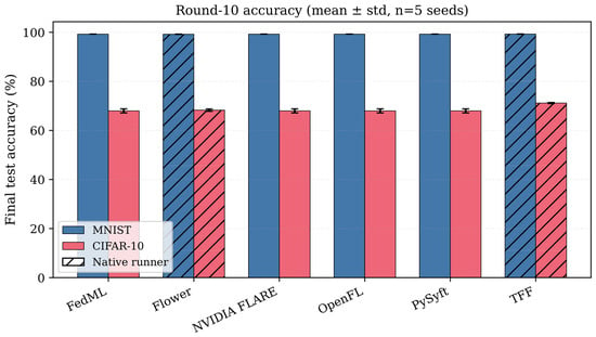
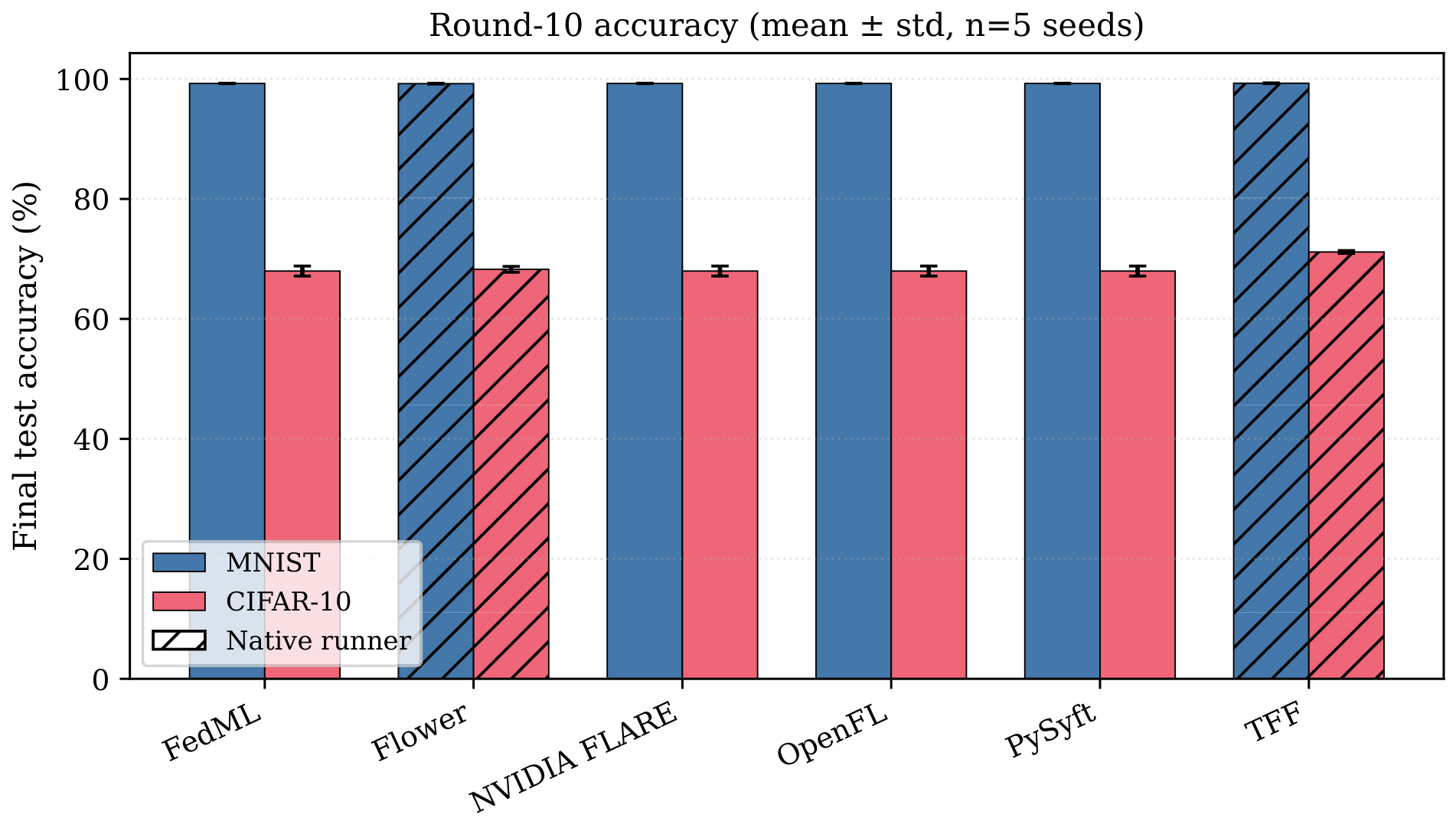
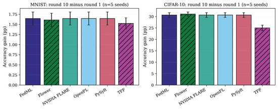
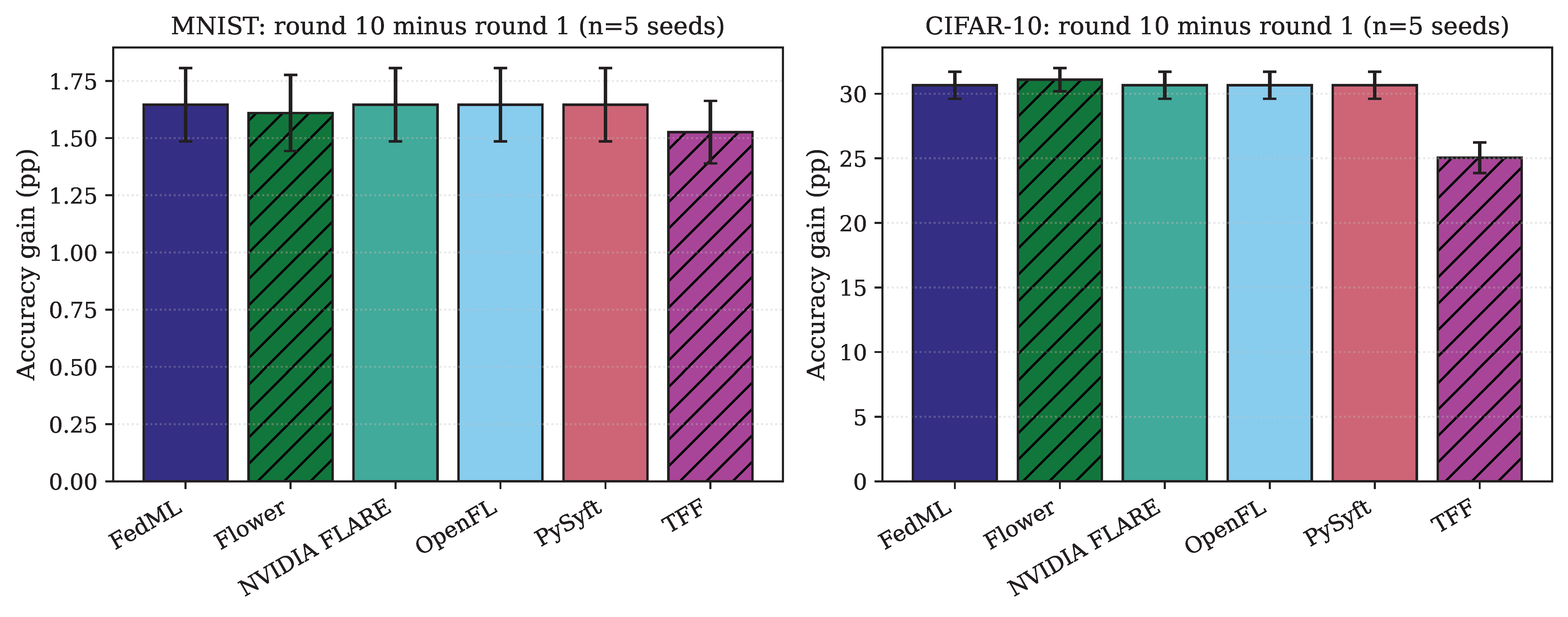
Figure 1 provides a high-level snapshot of round-10 test accuracy across both datasets. MNIST accuracies cluster above 99.2% for every framework; CIFAR-10 separates native TFF ($71.16\pm 0.23$%) from the PyTorch cluster (≈$68.0\pm 0.8$%). Figure 2 quantifies how much each framework improves from round 1 to round 10: CIFAR-10 gains are an order of magnitude larger (∼25–31 pp) than MNIST (∼1.6–1.9 pp), confirming that Phase 2 is the discriminative benchmark.

Figure 1. Final test accuracy (round 10) by framework for MNIST and CIFAR-10. Error bars: $\pm 1$ std over five seeds. Hatched bars: native runners.

Figure 2. Accuracy improvement from round 1 to round 10 (percentage points). (Left): MNIST; (right): CIFAR-10.

4.2. Phase 1: MNIST

Table 6 summarizes round-10 results (mean±std over five seeds). All frameworks converge to $99.22\pm 0.07$–$99.29\pm 0.06$% accuracy, validating that Equations (4) and (5) were implemented consistently. Wall time spans $21.8\pm 0.1$–$28.3\pm 0.6$ min: TFF and Flower are fastest among native runners on MNIST in this multi-seed batch; reference runners occupy a narrow $\sim 28$ min band.

Table 6. Phase 1: MNIST results (round 10, mean ± std, n = 5 seeds).

Framework	Impl.	Acc. (%)	Loss	Time (min)	Comm. (MB)
TFF	native	99.29 ± 0.06	0.020 ± 0.001	23.9 ± 0.1	761
FedML	ref.	99.26 ± 0.04	0.022 ± 0.000	27.9 ± 0.2	761
NVFlare	ref.	99.26 ± 0.04	0.021 ± 0.000	28.1 ± 0.2	761
OpenFL	ref.	99.26 ± 0.04	0.020 ± 0.000	28.2 ± 0.2	761
PySyft	ref.	99.26 ± 0.04	0.022 ± 0.000	28.3 ± 0.6	761
Flower	native	99.22 ± 0.07	0.023 ± 0.001	21.8 ± 0.1	761

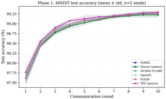
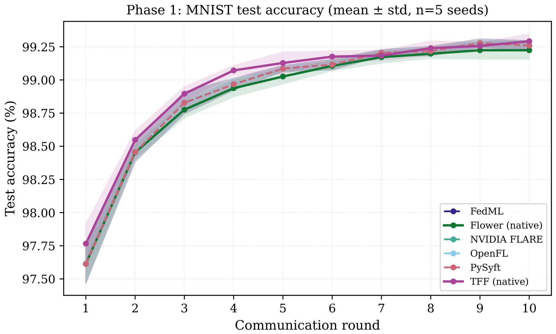
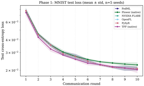
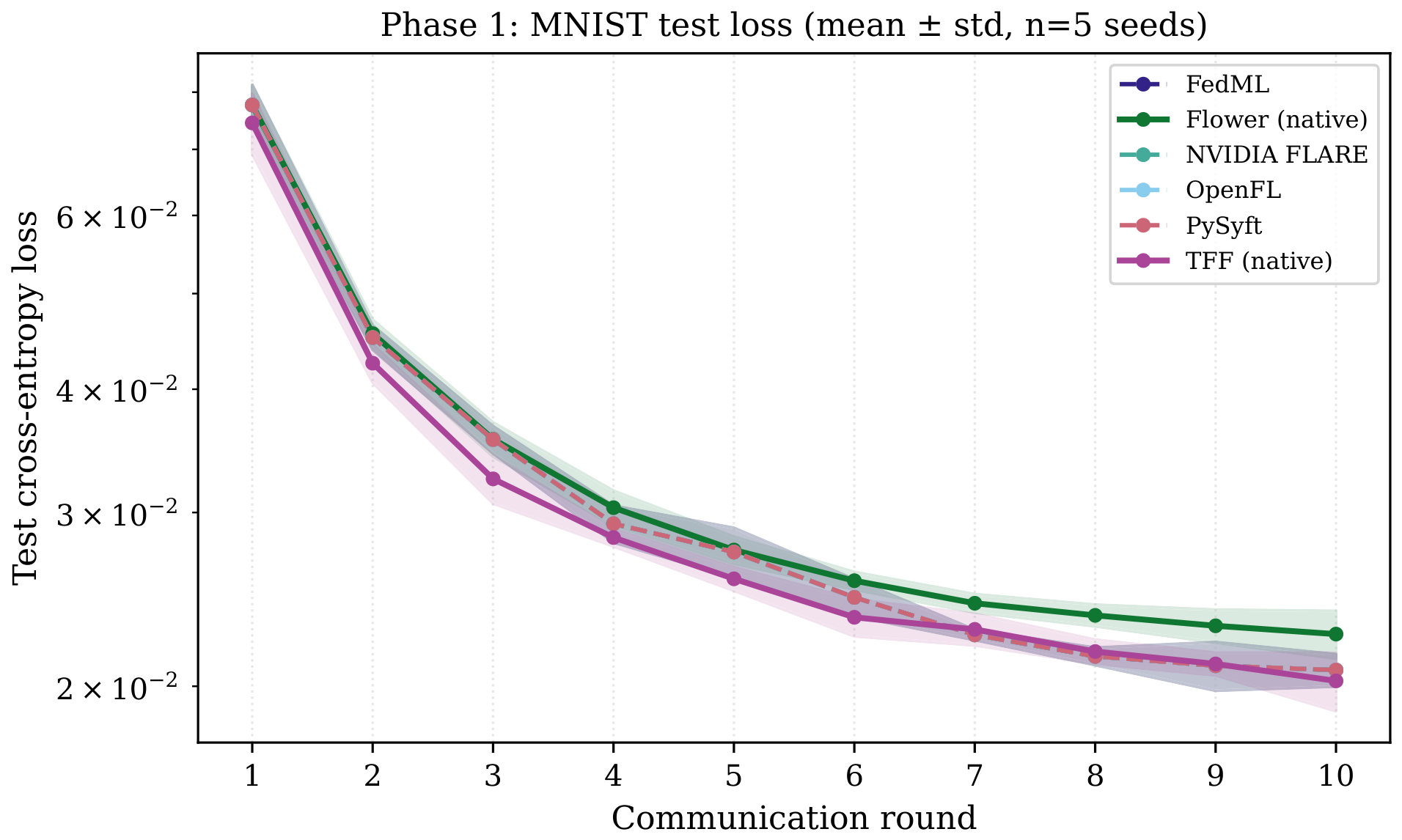
Figure 3 shows per-round accuracy with variability bands across seeds. Figure 4 reports cross-entropy loss. The near-overlap of reference-runner curves confirms that FedML, NVFlare, OpenFL, and PySyft execute the same underlying training loop on MNIST.

Figure 3. Global test accuracy versus communication round on MNIST (Phase 1). Lines: mean over five seeds; shaded: $\pm 1$ std.

Figure 4. Global test cross-entropy loss versus round on MNIST (Phase 1).

RQ1 (MNIST). Accuracy is framework-agnostic under IID MNIST (≤$0.07$ pp spread across framework means), but $T_{\mathrm{wall}}$ varies by $\sim 30$%. An earlier single-seed Flower MNIST run (42.1 min) is not representative of the five-seed mean ($21.8\pm 0.1$ min) and is discussed in Section 5. Reference runners occupy a $\sim 28$ min band. For 6G planners, orchestration overhead can dominate edge training schedules even when model quality is identical.

All runners report $C_{\mathrm{total}}\approx 761$ MB over ten rounds, consistent with Equation (6) for $K=6$ and $d=\mathrm{1,662,858}$ (Table 4).

4.3. Phase 2: CIFAR-10

Table 7 documents the operational outlier runs excluded according to the criteria in Section 3.8.

Table 7. Operational outlier runs excluded from aggregates (Section 3.8).

Framework	Dataset	Acc. (%)	Time (min)	Reason
Flower	CIFAR-10	68.23	164	Wall time $>3\times$ peer median; retained run 68.55%/17.9 min

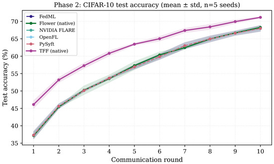
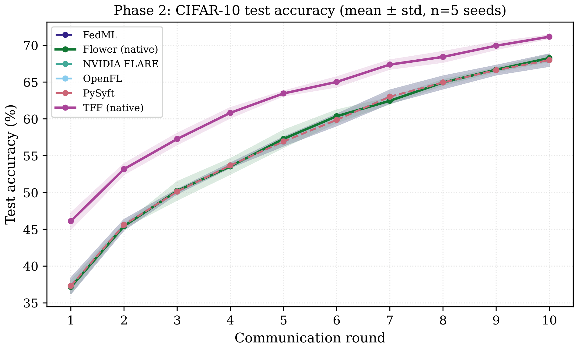
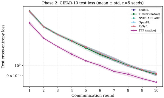
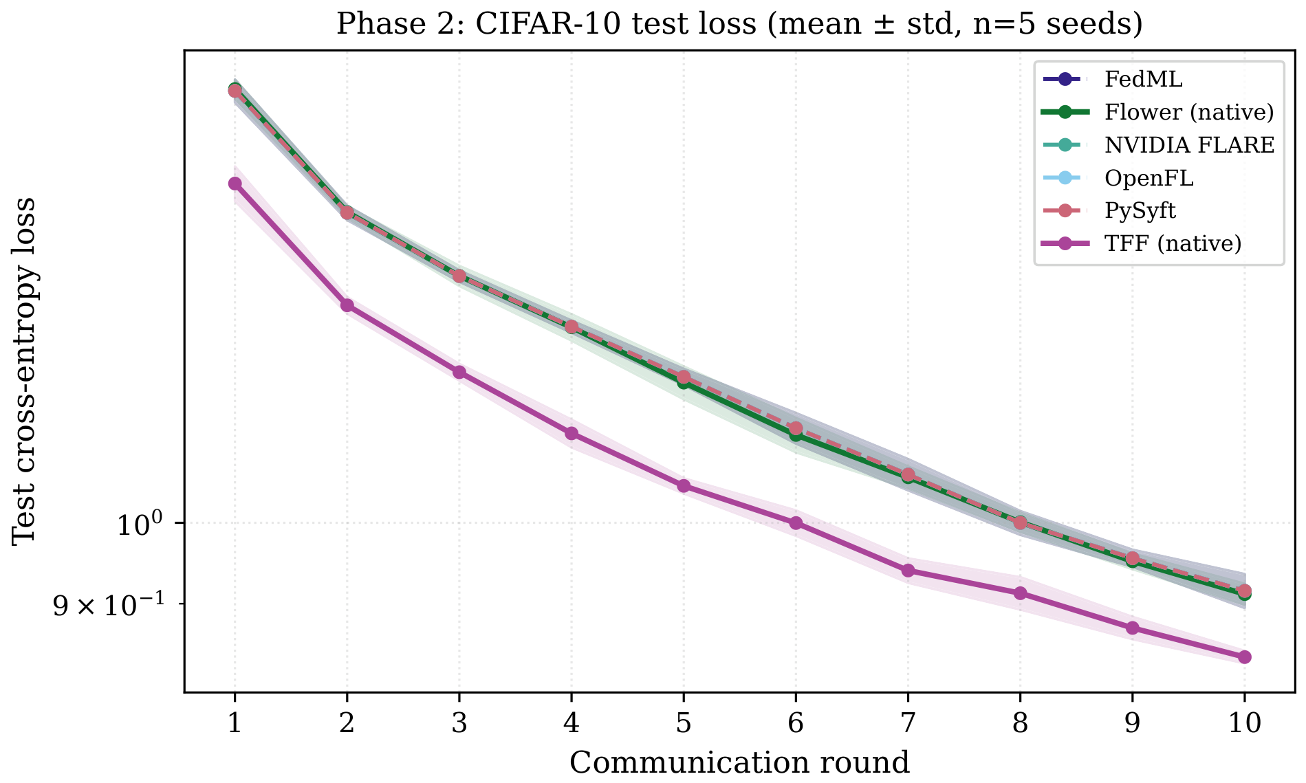
Table 8 and Figure 5 and Figure 6 report Phase 2 results (mean ± std, n = 5 seeds). Accuracy spread widens to ≈3.2 pp between TFF ($71.16\pm 0.23$%) and the reference cluster ($67.98\pm 0.84$%). Native Flower ($68.27\pm 0.49$%) aligns with references, not TFF.

Table 8. Phase 2: CIFAR-10 results (round 10, mean ± std, n = 5 seeds).

Framework	Impl.	Acc. (%)	Loss	Time (min)	Comm. (MB)
TFF	native	71.16 ± 0.23	0.82 ± 0.01	94.6 ± 47.7	268
Flower	native	68.27 ± 0.49	0.91 ± 0.01	17.7 ± 0.2	268
FedML	ref.	67.98 ± 0.84	0.89 ± 0.02	22.4 ± 0.3	268
NVFlare	ref.	67.98 ± 0.84	0.91 ± 0.02	22.3 ± 0.4	268
OpenFL	ref.	67.98 ± 0.84	0.93 ± 0.02	22.6 ± 0.3	268
PySyft	ref.	67.98 ± 0.84	0.92 ± 0.02	22.4 ± 0.5	268

Figure 5. Global test accuracy versus communication round on CIFAR-10 (Phase 2). Lines: mean over five seeds; shaded: $\pm 1$ std.

Figure 6. Global test cross-entropy loss versus round on CIFAR-10 (Phase 2).

TFF’s advantage appears from round 1 onward and persists in both accuracy and loss throughout training—suggesting a training-dynamics difference in the equivalent CNN rather than late-round aggregation effects.

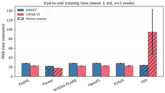
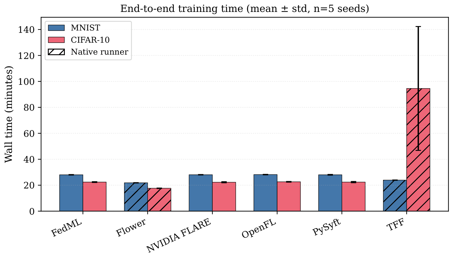
Wall times for PyTorch reference runners and Flower cluster near 22–24 min. TFF CIFAR-10 exhibits higher wall-time variance ($94.6\pm 47.7$ min) because one seed replicate exceeded our operational threshold (Table 7); excluding that replicate yields a reference-runner-comparable mean (∼66 min). Flower CIFAR-10 averages $17.7\pm 0.2$ min in the five-seed batch.

RQ2 (CIFAR-10). Framework rankings change relative to MNIST: TFF leads on accuracy ($+2.9$ pp over native Flower mean), while PyTorch reference wall times remain in a ∼22–24 min band. Phase 2 is therefore essential for framework discrimination in edge vision scenarios. All frameworks report $C_{\mathrm{total}}\approx 268$ MB over ten rounds, consistent with $d=\mathrm{586,250}$ in Table 4.

4.4. Cross-Phase Analysis: Time, Communication, and Heatmap

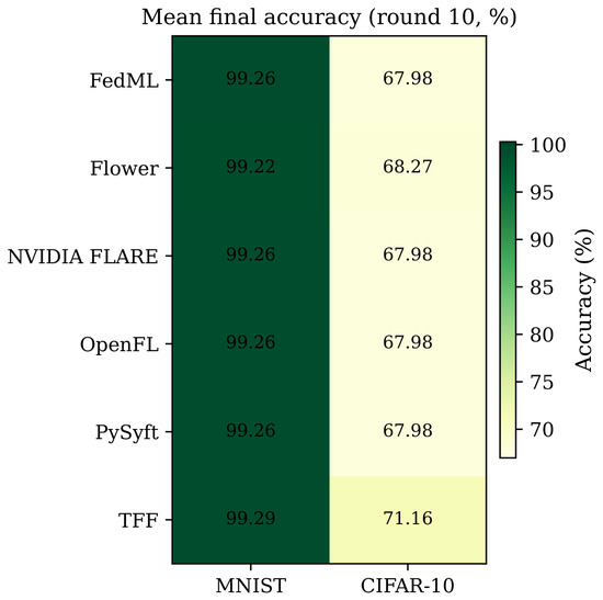
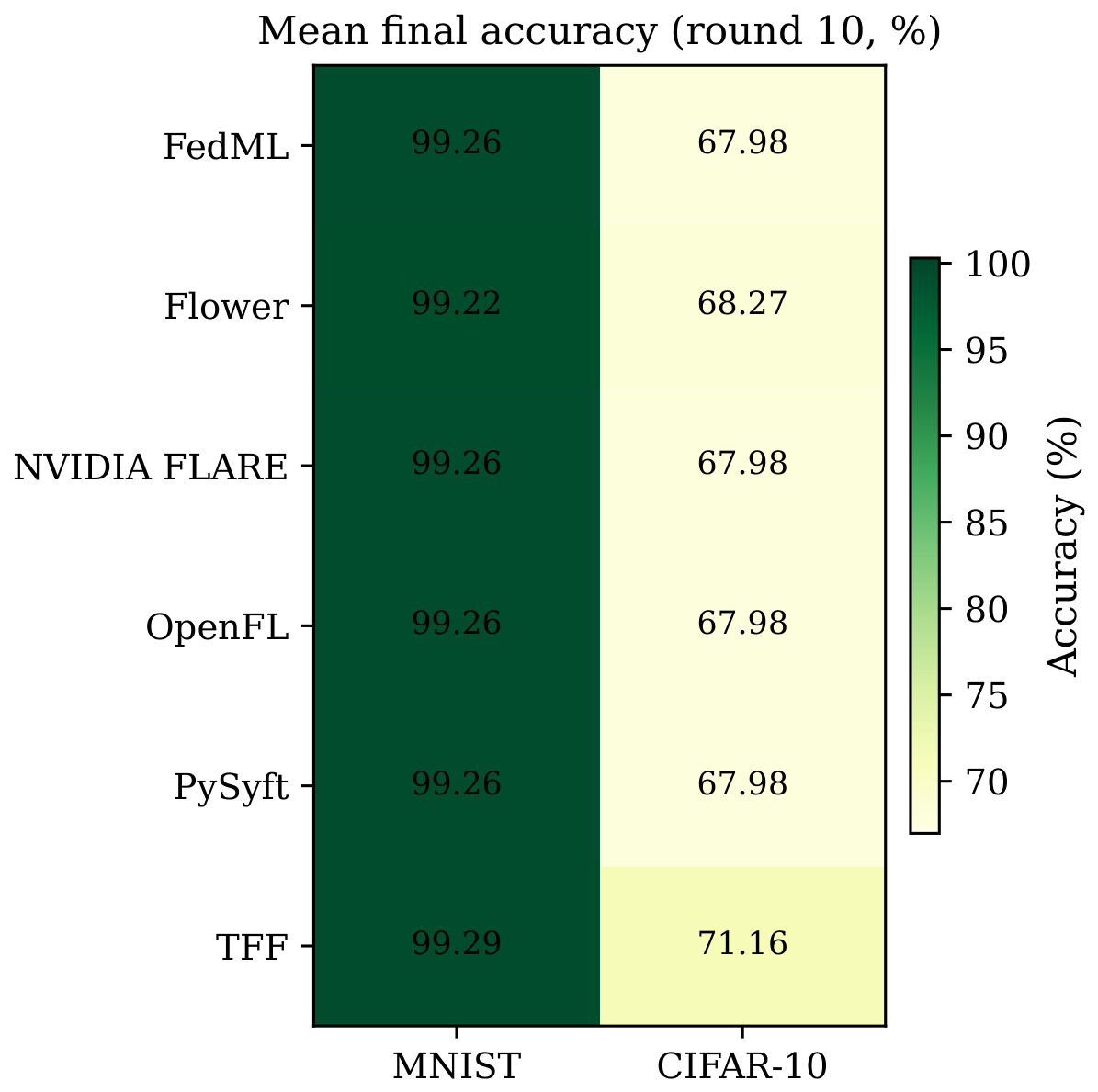
Figure 7 compares $T_{\mathrm{wall}}$ across datasets with error bars over five seeds. Multi-seed replication shows Flower MNIST at $21.8\pm 0.1$ min (not the 42.1 min single-seed anomaly from the original submission). Figure 8 summarizes final accuracies side-by-side: the MNIST column is uniformly green (≥99.2%), whereas the CIFAR-10 column reveals TFF as the clear leader.

Figure 7. End-to-end wall time by framework and dataset. Error bars: $\pm 1$ std over five seeds. Hatched bars: native runners.

Figure 8. Final test accuracy (round 10) across datasets and frameworks.

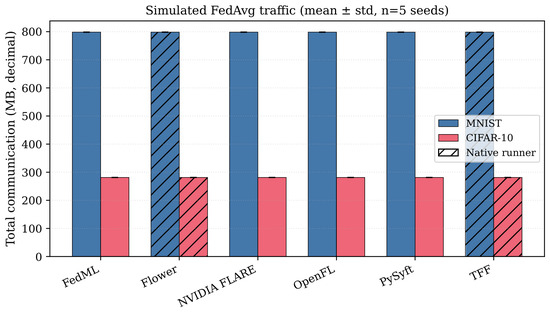
Figure 9 plots $C_{\mathrm{total}}$ for all six frameworks (RQ3). MNIST requires ∼2.8× more bytes than CIFAR-10 (761 vs. 268 MB, decimal megabytes) because the MNIST CNN yields larger ${\left|\mathbf{w}\right|}_{\mathrm{bytes}}$ despite smaller inputs. As a illustrative scheduling calculation only, if the full $C_{\mathrm{total}}$ were transferred sequentially on a symmetric 5 Mbps ($5\times {10}^6$ bit/s) ideal link with no protocol overhead, 268 MB would require at least ∼7.2 min of transfer time before compute; upload and download would be modelled separately under asymmetric 6G profiles.

Figure 9. Total simulated FedAvg communication over ten rounds (all frameworks; tensor-nbyte accounting).

Table 9 summarizes answers to the research questions.

Table 9. Research question summary.

RQ	Finding
RQ1	MNIST: equivalent accuracy (≈$99.26\%$ mean); native runners ≈ 22–24 min; reference ≈ 28 min.
RQ2	CIFAR-10: TFF leads by ≈$2.9$ pp; accuracy gaps emerge only under harder tasks.
RQ3	FedAvg: ≈761 MB (MNIST) and ≈268 MB (CIFAR-10) over ten ideal-network rounds (all frameworks).

5. Discussion

The narrow MNIST accuracy band across seeds and tight reference clustering on CIFAR-10 (≈68.0%) confirm consistent FedAvg (Equation (4)) and partitioning across runners. The TFF advantage on CIFAR-10 is treated as a hypothesis: TensorFlow/Keras optimization and numerical differences in the equivalent architecture may contribute [33], but we do not attribute it to a different aggregation rule. Centralized TensorFlow-versus-PyTorch ablations are left to future work.

For 6G edge deployment [3,7,19]: (1) use at least one non-trivial vision dataset before framework selection; (2) budget scheduling windows from measured $T_{\mathrm{wall}}$ including variance across seeds; and (3) plan uplink capacity using $C_{\mathrm{total}}$ from Equation (6) before applying bandwidth-limited or mMTC profiles [1,8,19].

Practitioner recommendations. If teams require TensorFlow-native training and can absorb longer CIFAR-10 runtimes, TFF delivers the highest accuracy in our locked FedAvg study. If PyTorch ecosystems are mandatory, Flower provides native orchestration with accuracy close to the shared reference cluster; FedML, NVFlare, OpenFL, and PySyft rows should be read as harness-validation baselines until native SDK paths are integrated. For MNIST-only smoke tests, any framework is adequate for correctness checks but insufficient for performance ranking.

Four frameworks share one PyTorch loop; comparing FedML, NVFlare, OpenFL, and PySyft on accuracy or bytes tests the runner, not product SDKs [12,13,14,17]. Flower and TFF remain the primary native comparison until reference runners are replaced. Fundamental limitations include the following: (i) standalone simulation does not capture WAN jitter, stragglers, or secure aggregation overhead; (ii) IID partitions do not reflect production non-IID telemetry; (iii) tensor-nbyte communication is a lower bound on wire traffic in distributed gRPC deployments. Future work will evaluate secure aggregation overhead [27,28], poisoning resilience [29,30], Dirichlet non-IID partitions, and 6G radio profiles (eMBB, URLLC, mMTC) on the same harness.

Limitations

Five random seeds per framework–dataset pair; ideal network only; IID partitions; tensor-nbyte communication (not packet capture); standalone simulation without distributed TLS/gRPC stress testing [27]; one hardware configuration; operational outliers excluded per Table 7. TFF CIFAR-10 wall-time variance remains high and warrants further profiling. Broader FL benchmarks such as FedScale [33] and LEAF [32] address different axes (scale, realism) and are complementary to our framework-centric study.

6. Conclusions

We presented a documented two-phase comparison of six federated learning frameworks on MNIST and CIFAR-10 with six IID clients, ten FedAvg rounds (Equations (3) and (4)), five random seeds per setting, and an ideal network profile on a Proxmox containerized testbed. Native Flower and TFF are compared against four reference-labelled runs of a shared PyTorch FedAvg harness. MNIST confirms protocol fairness (≈99.26% mean accuracy, ≤0.07 pp spread across framework means) but still reveals orchestration-time differences. CIFAR-10 exposes a documented accuracy lead for TFF ($71.16\pm 0.23$% vs. ≈$68.0\%$ for PyTorch runners) while reference wall times remain clustered near 22–24 min. Communication baselines (≈761 MB MNIST, ≈268 MB CIFAR-10, all frameworks) support upcoming 6G constraint and security studies [7,30].

For the 6G and edge-intelligence communities, the study demonstrates that (i) easy datasets alone are insufficient for framework ranking, (ii) explicit native-versus-reference labelling is necessary when SDK integrations are uneven, and (iii) public per-round metrics enable independent verification. Planned extensions on the same harness include Dirichlet non-IID data [23,24], IMT-2030 radio profiles (eMBB, URLLC, mMTC) [1,3,4], secure aggregation [27], and adversarial robustness evaluations [29].

References

- International Telecommunication Union. IMT-2030: Technical Requirements for the 6G Future. 2026. Available online: https://www.itu.int/hub/2026/03/imt-2030-technical-requirements-for-the-6g-future/ (accessed on 4 August 2026).
- 3rd Generation Partnership Project (3GPP). Release 20. 2026. Available online: https://www.3gpp.org/specifications-technologies/releases/release-20 (accessed on 4 August 2026).
- Saad, W.; Bennis, M.; Chen, M. A Vision of 6G Wireless Systems: Applications, Trends, Technologies, and Open Research Problems. IEEE Netw. 2020, 34, 134–142. [Google Scholar] [CrossRef] [Scilit]
- Letaief, K.B.; Chen, W.; Shi, Y.; Zhang, J.; Zhang, Y.J.A. The Roadmap to 6G: AI Empowered Wireless Networks. IEEE Commun. Mag. 2019, 57, 84–90. [Google Scholar] [CrossRef] [Scilit]
- Zhou, Z.; Chen, X.; Li, E.; Zeng, L.; Luo, J.; Zhang, J. Edge Intelligence: Paving the Last Mile of Artificial Intelligence with Edge Computing. Proc. IEEE 2019, 107, 1738–1762. [Google Scholar] [CrossRef] [Scilit]
- Shi, W.; Cao, J.; Zhang, Q.; Li, Y.; Xu, L. Edge Computing: Vision and Challenges. IEEE Internet Things J. 2016, 3, 637–646. [Google Scholar] [CrossRef] [Scilit]
- Lim, W.Y.B.; Luong, N.C.; Hoang, D.T.; Jiao, Y.; Liang, Y.C.; Yang, Q.; Niyato, D.; Miao, C. Federated Learning in Mobile Edge Networks: A Comprehensive Survey. IEEE Commun. Surv. Tutor. 2020, 22, 2031–2063. [Google Scholar] [CrossRef] [Scilit]
- Park, J.; Samarakoon, S.; Bennis, M.; Debbah, M.; Poor, H.V.; Shroff, N.B. Wireless Network Intelligence at the Edge. Proc. IEEE 2019, 107, 2204–2235. [Google Scholar]
- McMahan, H.B.; Moore, E.; Ramage, D.; Hampson, S.; y Arcas, B.A. Communication-Efficient Learning of Deep Networks from Decentralized Data. In 20th International Conference on Artificial Intelligence and Statistics (AISTATS); Pmlr: London, UK, 2017; pp. 1273–1282. [Google Scholar]
- Kairouz, P.; McMahan, H.B. Advances and Open Problems in Federated Learning. Found. Trends Mach. Learn. 2021, 14, 1–210. [Google Scholar] [CrossRef] [Scilit]
- Yang, Q.; Liu, Y.; Chen, T.; Tong, Y. Federated Machine Learning: Concept and Applications. ACM Trans. Intell. Syst. Technol. 2019, 10, 1–19. [Google Scholar] [CrossRef] [Scilit]
- He, C.; Li, S.; So, J.; Bian, Z.; Wang, M.; Zhao, H.; Zeng, H.; Li, Z.; Li, Y.; Chen, Y.; et al. FedML: A Research Library and Benchmark for Federated Machine Learning. In Proceedings of the NeurIPS Workshop on Federated Learning, Virtual, 11 December 2020. [Google Scholar]
- Roth, H.; Cheng, Y.; Wen, Y.; Yang, I.; Xu, Z.; Hsieh, Y.T.; Kersten, K.; Harouni, A.; Zhao, C.; Li, W.; et al. NVIDIA FLARE: Federated Learning from Simulation to Real-World. arXiv 2022, arXiv:2210.13291. [Google Scholar]
- Ryffel, T.; Trask, A.; Dahl, B.; Wagner, B.; Mancuso, J.; Rueckauer, J.; Mazzone, D.; Onuigbo, I.; Platt, D.; Wergan, N.; et al. A Generic Framework for Privacy Preserving Deep Learning. arXiv 2018, arXiv:1811.04017. [Google Scholar]
- Beutel, D.J.; Topal, T.; Mathur, A.; Qiu, T.; Parcollet, T.; Lane, N.D.; McMahan, H.B.; Ramage, D. Flower: A Friendly Federated Learning Framework. arXiv 2020, arXiv:2007.14390. [Google Scholar]
- Google LLC. TensorFlow Federated. Version 0.85.0 Used in Experiments. 2024. Available online: https://www.tensorflow.org/federated (accessed on 4 August 2026).
- Foley, P.; Sheller, M.J.; Edwards, B.; Pati, S.; Riviera, W.; Sharma, M.; Narayana Moorthy, P.; Wang, S.H.; Martin, J.; Mirhaji, P.; et al. OpenFL: The Open Federated Learning Library. Phys. Med. Biol. 2022, 67, 214001. [Google Scholar] [CrossRef] [Scilit] [PubMed]
- Konečnỳ, J.; McMahan, H.B.; Ramage, D.; Drágu, P. Federated Learning: Strategies for Improving Communication Efficiency. In Proceedings of the NeurIPS Workshop on Private Multi-Party Machine Learning, Barcelona, Spain, 9 December 2016. [Google Scholar]
- Yang, Z.; Chen, M.; Wong, K.K.; Poor, H.V.; Cui, S. Federated Learning for 6G: Applications, Challenges, and Opportunities. Engineering 2022, 8, 33–41. [Google Scholar] [CrossRef] [Scilit]
- Wang, J.; Liu, Q.; Liang, H.; Joshi, G.; Poor, H.V. A Field Guide to Federated Optimization. arXiv 2021, arXiv:2107.06917. [Google Scholar]
- Krizhevsky, A. Learning Multiple Layers of Features from Tiny Images; Technical Report; University of Toronto: Toronto, ON, Canada, 2009. [Google Scholar]
- Li, T.; Sahu, A.K.; Talwalkar, A.; Smith, V. Federated Learning: Challenges, Methods, and Future Directions. IEEE Signal Process. Mag. 2020, 37, 50–60. [Google Scholar] [CrossRef] [Scilit]
- Zhao, Y.; Li, M.; Lai, L.; Park, N.; Wang, T.; Paulik, B.; Singh, A.; Yousif, K. Federated Learning with Non-IID Data. In Proceedings of the ICLR Workshop, Vancouver, BC, Canada, 30 April–3 May 2018. [Google Scholar]
- Li, T.; Sahu, A.K.; Zaheer, M.; Sanjabi, M.; Talwalkar, A.; Smith, V. Federated Optimization in Heterogeneous Networks. In Proceedings of the MLSys; mlsys.org: Austin, TX, USA, 2020; pp. 429–450. [Google Scholar]
- Karimireddy, S.P.; Kale, S.; Mohri, M.; Reddi, S.; Stich, S.; Suresh, A.T. SCAFFOLD: Stochastic Controlled Averaging for Federated Learning. In Proceedings of the ICML; Curran Associates, Inc.: Red Hook, NY, USA, 2020; pp. 5132–5143. [Google Scholar]
- Stich, S.U. Local SGD Converges Fast and Communicates Little. In Proceedings of the ICLR, New Orleans, LA, USA, 6–9 May 2019. [Google Scholar]
- Bonawitz, K.; Ivanov, V.; Kreuter, B.; Marcedone, A.; McMahan, H.B.; Patel, S.; Ramage, D.; Segal, A.; Seth, K. Practical Secure Aggregation for Privacy-Preserving Machine Learning. In Proceedings of the CCS; ACM: New York, NY, USA, 2017; pp. 1175–1191. [Google Scholar]
- Geyer, R.C.; Klein, T.; Nabi, M. Differentially Private Federated Learning: A Client Level Perspective. arXiv 2017, arXiv:1712.07557. [Google Scholar]
- Bagdasaryan, E.; Veit, A.; Hua, Y.; Na, S.; Shmatikov, V. How to Backdoor Federated Learning. In Proceedings of the AISTATS; JMLR, Inc.: Cambridge, MA, USA, 2020; pp. 2938–2948. [Google Scholar]
- Lyu, L.; Yu, H.; Yang, Q. Threats to Federated Learning: A Survey. arXiv 2020, arXiv:2003.02133. [Google Scholar]
- Kaissis, G.; Ziller, A.; Passerat-Palmbach, J.; Ryffel, T.; Usynin, D.; Trask, A.; Lima, I.; Mancuso, J.; Jungmann, F.; Steinborn, M.M.; et al. End-to-end privacy preserving deep learning on multi-institutional medical imaging. Nat. Mach. Intell. 2021, 3, 473–484. [Google Scholar] [CrossRef] [Scilit]
- Caldas, S.; Konečnỳ, J.; McMahan, H.B.; Talwalkar, A. LEAF: A Benchmark for Federated Settings. arXiv 2018, arXiv:1812.01097. [Google Scholar]
- Lai, F.; Dai, Y.; Singapuram, S.S.; Liu, J.; Zhu, X.; Madhyastha, H.V.; Chowdhury, M. FedScale: Benchmarking Model and System Performance of Federated Learning at Scale. In Proceedings of the 39th International Conference on Machine Learning (ICML); Proceedings of Machine Learning Research: London, UK, 2022; Volume 162, pp. 11814–11827. [Google Scholar]
- Liang, Y.; Guo, Y.; Gong, Y.; Luo, C.; Zhan, J.; Huang, Y. FLBench: A Benchmark Suite for Federated Learning. arXiv 2021, arXiv:2008.07257. [Google Scholar]
- Ogier du Terrail, J.; Ayed, S.S.; Cyffers, E.; Grimberg, F.; He, C.; Loeb, R.; Mangold, P.; Marchand, T.; Marfoq, O.; Mushtaq, E.; et al. FLamby: Datasets and Benchmarks for Cross-Silo Federated Learning in Realistic Healthcare Settings. Adv. Neural Inf. Process. Syst. 2022, 35, 5315–5334. [Google Scholar] [CrossRef] [Scilit]
- Mattson, P.; Cheng, C.; Diamos, G.; Coleman, C.; Micikevicius, P.; Patterson, D.; Tang, H.; Wei, G.Y.; Bailis, P.; Bittorf, V.; et al. MLPerf Training Benchmark. Proc. Mach. Learn. Syst. 2019, 1, 336–349. [Google Scholar]
- Batsios, V.D.; Angelis, C.T. FL Framework Performance Benchmark for 6G Wireless Scenarios—Public Results. GitHub Results Repository. 2026. Available online: https://github.com/vasileiosbatsios/phd_6g_federated_learning (accessed on 1 August 2026).
- LeCun, Y.; Bottou, L.; Bengio, Y.; Haffner, P. Gradient-Based Learning Applied to Document Recognition. Proc. IEEE 1998, 86, 2278–2324. [Google Scholar] [CrossRef] [Scilit]
- LeCun, Y.; Bengio, Y.; Hinton, G. Deep Learning. Nature 2015, 521, 436–444. [Google Scholar] [CrossRef] [Scilit] [PubMed]
- Felter, W.; Ferreira, A.; Rajamony, R.; Rubio, J. An Updated Performance Comparison of Virtual Machines and Linux Containers. In Proceedings of the 2015 IEEE International Symposium on Performance Analysis of Systems and Software (ISPASS); IEEE: New York, NY, USA, 2015; pp. 171–172. [Google Scholar] [CrossRef] [Scilit]
Disclaimer/Publisher’s Note: The statements, opinions and data contained in all publications are solely those of the individual author(s) and contributor(s) and not of MDPI and/or the editor(s). MDPI and/or the editor(s) disclaim responsibility for any injury to people or property resulting from any ideas, methods, instructions or products referred to in the content. |
© 2026 by the authors. Licensee MDPI, Basel, Switzerland. This article is an open access article distributed under the terms and conditions of the Creative Commons Attribution (CC BY) license.