DP-RVFL: A Differentially Private Randomized-Feature Neural Model for Privacy–Utility Efficient Learning

Abstract

Differentially private stochastic gradient descent (DP-SGD) enables neural network training with formal privacy guarantees, but its utility depends on model architecture, data modality, and privacy budget. DP-RVFL freezes random hidden features and privately trains an output layer with a direct input connection. We compare it with Dense/CNN models, no-link and parameter-matched frozen controls, logistic regression and published DP-ELM. MNIST, CIFAR-10, Cardio and Heart are evaluated at ε = 0.1–8 using five training seeds. Gaussian gradient models use Poisson sampling, Adam, δ = 10⁻⁵ and add/remove-one adjacency. Primary ε = 2 accuracies are 90.30%, 38.61%, 72.99% and 63.48%, respectively. CIFAR-10 training takes 71.29 s versus 529.76 s for DP-CNN using eight CPU threads. DP-RVFL exceeds the no-link mean accuracy in 20 of 24 primary conditions, but the matched frozen control in only eight. Two additional executions preserve the same configuration and are reported separately. Five-pair exact tests do not establish statistical superiority. Diagnostics do not substantiate a reduced-clipping explanation, and Heart results vary across small partitions. The evidence supports lower training time relative to the tested Dense/CNN models; privacy budgets apply per model conditional on public benchmark preparation.

1. Introduction

Training neural networks on sensitive records raises the question of how to limit record disclosure while preserving predictive utility. Even when raw training data are not directly released, trained models may still leak private information through model parameters, prediction confidence scores, or gradients. Previous studies have examined membership inference and training data extraction, where an adversary attempts to determine whether a record was used during training or recover sensitive information from a trained model [1,2].

Differential privacy provides a formal framework for limiting the influence of any individual record on the output of a computation. Its definition bounds differences between output distributions on neighboring datasets [3,4]. In deep learning, differentially private stochastic gradient descent, commonly known as DP-SGD, is a foundational method for training neural networks under differential privacy. DP-SGD modifies standard gradient-based optimization by clipping per-example gradients, adding calibrated Gaussian noise, and tracking the accumulated privacy loss using a privacy accountant [5].

DP-SGD has been applied to benchmark image datasets such as MNIST [6] and CIFAR-10 [7], and it remains a standard baseline for private deep learning [5]. However, the use of gradient clipping and noise injection introduces a clear privacy–utility trade-off. Stronger privacy settings usually require more noise, which may reduce accuracy, slow convergence, and increase training instability. This effect becomes more challenging when the dataset is small, the model has many trainable parameters, or the task requires fine-grained decision boundaries.

Restricting the update to an output layer changes the optimization problem. It does not by itself reduce the reported privacy budget or guarantee higher predictive accuracy.

In this setting, this paper presents a comparative privacy–utility evaluation of three neural architecture families: Dense networks, Convolutional Neural Networks, and Random Vector Functional Link style randomized-feature networks. Each architecture is evaluated in both non-private and differentially private forms. The private models are referred to as DP-Dense, DP-CNN, and DP-RVFL. All private models are trained using the same DP-SGD privacy-budget settings, ranging from strict privacy to weaker privacy levels. This enables a comparison under matched per-run privacy budgets and a common, prespecified training schedule. Additional controls are defined below.

Random vector functional link (RVFL) networks combine fixed random nonlinear features with direct input-to-output connections. Randomized functional-link networks and extreme learning machines (ELMs) precede the present study [8,9,10]. Differentially Private Extreme Learning Machine (DP-ELM), introduced by Ono et al., also uses a fixed random hidden layer, but privatizes sufficient statistics before solving for the output coefficients [11]. Thus, neither frozen random features nor private training of their output coefficients is claimed here as a new principle. The empirical question is whether the direct input path in a DP-SGD-trained RVFL changes utility and training time relative to appropriate controls under the same specified protocol.

We examine that question with two distinct comparisons. A no-direct-link model retains the same random hidden features and trains its output layer using the same gradient-sanitization mechanism. A second frozen random network expands its hidden width to match the RVFL output layer’s trainable parameter count. Raw-input and projected-input logistic regression distinguish a linear representation from the addition of random nonlinear features. Published DP-ELM is evaluated separately because its loss, activation, hidden widths and pure-DP mechanism differ from those of the gradient-trained models.

The evaluation is conducted on four datasets representing two different data modalities. MNIST and CIFAR-10 are used as standard image classification benchmarks, while two cardiovascular tabular datasets are used as public binary-classification benchmarks. For image datasets, CNNs are naturally suitable because they exploit spatial structure. For tabular datasets, Dense and RVFL-style models are expected to be more appropriate, while the CNN is implemented as a one-dimensional feature-based convolutional model for exploratory comparison. The datasets are trained and evaluated separately; images are not used to predict cardiovascular outcomes, and records from different datasets are not combined. This design does not establish clinical transportability.

The study specifies the adjacency relation, sampling process, exact accounting schedule, fixed preprocessing and model-selection policy; evaluates the direct-link, frozen-feature and logistic controls; and measures training time alongside trainable parameters, forward-operation estimates and stored parameter bytes. Additional analyses examine fixed image transformations, public gradient diagnostics, alternative Heart partitions and a compact attention classifier. Two additional executions of the same suite are reported separately as repeatability checks. The contribution is a controlled, auditable benchmark comparison, with conclusions restricted to the tested architectures and optimization schedules.

The remainder of this paper is organized as follows. Section 2 reviews related work on differentially private deep learning, private fixed-feature classifiers, and randomized-feature neural networks. Section 3 presents the methodology, including the formal definition of differential privacy, the DP-SGD training mechanism, the baseline Dense and CNN architectures, and the DP-RVFL model and comparison controls. Section 4 presents experimental evaluation and discussion. Section 5 concludes the paper and outlines directions for future research.

2. Related Work

2.1. Private Gradient Training and Fixed-Feature Classifiers

The DP-SGD construction of Abadi et al. combines gradient clipping, randomized sampling, Gaussian perturbation and privacy accounting [5]. Rényi differential privacy (RDP) provides a composition framework, and the sampled Gaussian mechanism requires an analysis consistent with the actual subsampling rule [12,13]. Opacus implements per-example gradient processing and privacy accounting in PyTorch [14]. In the present implementation, Poisson sampling, a fixed public normalization and an exact number of accountant steps are specified explicitly. The privacy claim concerns the mechanism; prediction error is not used as a proxy for privacy.

Private logistic regression is an established baseline. Chaudhuri et al. analyze output and objective perturbation for private empirical risk minimization, including logistic classification [15]. Giddens et al. consider differentially private weighted empirical risk minimization [16]. Our logistic controls use the same Poisson-sampled Gaussian gradient mechanism as DP-RVFL, rather than reproducing those output- or objective-perturbation algorithms. This choice holds the optimizer, clipping and accountant constant when examining the representation.

2.2. RVFL, ELM and Published DP-ELM

The direct link distinguishes the RVFL feature vector, which concatenates inputs and random nonlinear features, from an ELM-style hidden-only representation [8,9,10]. Classical ELM determines output coefficients analytically [17]. Here, the hidden-only ablation is named ELM-SGD, or DP-ELM-SGD under private training, to distinguish its gradient-trained classifier from a closed-form ELM.

Ono et al.’s DP-ELM adds independent Laplace perturbations to entries of H^TH and H^TY and solves the resulting linear system [11]. Its analysis uses sigmoid hidden units, one-hot targets and pure ε-DP under replace-one adjacency. DP-RVFL instead concatenates a direct path with tanh random features and applies approximate (ε, δ)-DP gradient training to a logistic/softmax output layer. These differences are stated explicitly because an accuracy difference between the complete methods cannot identify the direct link as its sole explanation. The same-mechanism DP-ELM-SGD comparison is the direct-link ablation; the published-mechanism DP-ELM comparison places that ablation in its literature context.

2.3. Security Scope and Stronger Image-Training Configurations

Random feature selection has also been studied for adversarial-transfer defenses. Nowroozi et al. select deep features and evaluate attack transfer on UNSW-NB15 [18]. That threat model concerns adversarial manipulation, whereas the present study concerns training-record privacy. We cite this work to distinguish these uses of randomization. Our frozen Dense control does not reproduce its defense, and our experiments do not establish resistance to poisoning or evasion attacks.

The evaluated small networks are not the highest-accuracy available private image classifiers. De et al. report 81.4% CIFAR-10 accuracy at (8, 10⁻⁵)-DP using a substantially different Wide-ResNet training configuration, including larger batches and augmentation multiplicity [19]. That published result is the literature context, not a reproduced baseline or a matched runtime comparison. It also precludes interpreting the present low CIFAR-10 accuracies as an intrinsic limit of differential privacy. Medical imaging studies such as Ziller et al. evaluate DP in a different application setting [20]; public cardiovascular tables do not substitute for that type of application-specific evaluation.

3. Methodology

This study evaluates DP-RVFL, a differentially private randomized-feature neural model designed to reduce the dimensionality of the parameter space subjected to private optimization. Unlike fully trainable neural networks, DP-RVFL generates a randomized hidden representation independently of the private training data and keeps this representation fixed throughout training. Differentially private stochastic gradient descent (DP-SGD) is then applied only to the output-layer parameters.

To evaluate the architecture, two conventional neural model families are used as comparison baselines: a fully connected Dense network and a Convolutional Neural Network (CNN). Each architecture is evaluated in conventional and differentially private forms. The private variants are denoted as DP-Dense, DP-CNN, and DP-RVFL. The three architectures are trained and evaluated independently; they are not integrated into a single hybrid model. Additional frozen-feature, logistic and published DP-ELM controls are described in Section 3.5.

The main methodological distinction is that DP-Dense and DP-CNN privately optimize their complete trainable representations, whereas DP-RVFL restricts data-dependent private optimization to a compact output layer. This reduction does not directly produce a smaller formal privacy budget. Instead, it reduces the dimensionality of the optimization problem subjected to per-example gradient clipping and Gaussian perturbation. The following subsections define differential privacy, describe the DP-SGD mechanism, and present the evaluated architectures, with particular emphasis on the DP-RVFL model.

3.1. Privacy Definition and Release Scope

Differential privacy provides a formal framework for limiting the influence of any individual record on the output of a randomized computation [3,4].

Let D and D′ differ by the addition or removal of one prepared training record. A randomized training mechanism M is (ε, δ)-differentially private if, for every measurable output event S,

$$\begin{array}{c}\mathrm{Pr}\left[M\left(D\right)\in S\right]\le e^{ϵ}\mathrm{Pr}\left[M\left(D^{\prime }\right)\in S\right]+\delta .\end{array}$$

(1)

The parameter ε represents the privacy budget and bounds the multiplicative difference between the output distributions obtained from neighboring datasets. Smaller values of ε correspond to stronger privacy because the output becomes less dependent on any individual record. The additive slack δ relaxes the distributional bound; it is not the probability that a particular person is exposed. Add/remove-one is the adjacency relation used for all Gaussian mechanism experiments; no interchangeable replace-one guarantee is asserted for those runs.

The guarantee is conditional on fixed, public benchmark preparation, partition specifications and protocol parameters. A public reference size N₀ determines the sampling rate, number of steps and gradient normalizer; these values are held fixed when comparing neighboring training inputs. The numerical count is not re-estimated on a confidential neighboring population. Random feature maps and projection seeds are independent of record values. Recordwise fixed transforms require no fitted population statistics, but the raw-file cleaning, cohort construction, partition audit and class-count reports in this benchmark pipeline are not claimed to be private.

Each reported privacy budget applies to one released trained model. Releasing multiple models trained on overlapping confidential records would require composition across those releases. The entire sweep, its two repeated executions, and its raw training diagnostics do not inherit a single per-run ε. Test metrics are evaluated on public benchmark records. The separate diagnostic stage exports non-private losses and clipping statistics and must not be treated as a confidential-data release procedure.

3.2. Poisson Sampling, Sanitized Gradients and Accounting

DP-SGD extends conventional stochastic gradient descent by bounding the contribution of each individual training sample and perturbing the aggregated gradient with Gaussian noise [5].

For requested batch size B and E epochs, define J = ⌈N₀/B⌉, sampling rate q = 1/J, total updates T = EJ, and fixed normalizer m₀ = max(1, ⌊qN₀⌋). Each record is included independently at each update,

B_t = {z_i ∈ D:I_i,t = 1},I_i,t∼Bernoulli(q)

(2)

where independent Bernoulli indicators produce variable-size Poisson batches B_t. These are not fixed-size shuffled mini-batches. For each sampled record, the loss gradient with respect to the trainable parameters is

$$\begin{array}{c}{g}_i={\nabla }_{\theta }L\left({\theta }_t;x_i,y_i\right)\end{array}$$

(3)

Each per-example gradient is clipped to a maximum L2-norm C:

$$\begin{array}{c}{\overline{g}}_i=g_i\min \left(1,{\displaystyle \frac{C}{{\parallel g_i\parallel }_2}}\right).\end{array}$$

(4)

Gradient clipping ensures that no individual record can contribute an arbitrarily large gradient to the model update. The clipped gradients are subsequently aggregated, and calibrated Gaussian noise is added. The clipped sum is divided by the fixed normalizer m₀:

$${\tilde{g}}_t={\displaystyle \frac{\sum _{i\in B_t}{\overline{g}}_i+{\xi }_t}{m_0}},{\xi }_t\sim \mathcal{N}\left(0,{\sigma }^2{C}^{2}I\right)$$

(5)

where C = 1 is the clipping threshold and σ is the calibrated noise multiplier. Under add/remove-one adjacency, the clipped sum has sensitivity at most C conditional on previous private outputs. The denominator m₀ is fixed, rather than the realized random batch size. An empty batch still produces a noise-only optimizer update and an accountant step.

The implementation uses Adam [21] on the sanitized gradients. Equation (6) specifies the update operator, where s_t contains the first- and second-moment state and step counter, rather than an ordinary SGD update:

$${\theta }_{t+1}={\mathrm{Adam}}_{\eta ,{\beta }_1,{\beta }_2}\left({\theta }_t,{\tilde{g}}_t;s_t\right)$$

(6)

The Adam moments depend on sanitized gradients; they do not access unnoised gradients outside the private optimizer. The term DP-SGD in this manuscript identifies the sampling, clipping and Gaussian gradient mechanism, with Adam as its update rule. The learning rate is 0.001, β₁ = 0.9, β₂ = 0.999, the Adam denominator constant is 10⁻⁸, and weight decay is zero.

The Gaussian perturbation randomizes the contribution of individual training examples, while gradient clipping bounds the sensitivity of each optimization step. Because multiple private updates are performed during training, the cumulative privacy loss is tracked using a privacy accountant. In this work, Rényi differential privacy accounting is used to calculate the achieved ε for the selected value of δ [12].

The resulting privacy guarantee depends principally on the sampling rate, noise multiplier, number of optimization steps, and δ. The number of model parameters does not directly determine the value of ε. However, architecture design determines how many parameters and gradient coordinates are subjected to clipping, perturbation, and private iterative optimization. This distinction motivates restricting DP-SGD to the final output layer in DP-RVFL.

The noise multiplier is calibrated before training using the Opacus RDP accountant for the implemented q, exact T and δ. Binary search uses an ε tolerance of 10⁻⁴, and calibration is accepted only when the computed ε does not exceed its target. The order set is {1.1, 1.2, …, 10.9} ∪ {12, 13, …, 255} ∪ {256, 512, 1024, 2048, 4096, 8192, 16,384}. The accountant composes the sampled Gaussian steps and converts the accumulated RDP bounds to (ε, δ)-DP [12,13]. The final accountant history, completed steps and achieved ε are checked against the calibrated protocol. Table S3 records the resulting multipliers and achieved budgets. Opacus secure mode is enabled with torchcsprng; the public model seeds do not deterministically reproduce its private noise.

3.3. Trained Dense and CNN Baselines

The Dense network is used as a fully connected baseline for both image and tabular classification. For MNIST and CIFAR-10, each input image is flattened into a one-dimensional feature vector before being supplied to the fully connected layers. For the Cardio and Heart datasets, the preprocessed tabular feature vector is used directly as the network input.

For the binary cardiovascular classification tasks, the Dense architecture contains two fully connected hidden layers with 64 and 32 neurons, respectively. A rectified linear unit activation is applied after each hidden layer, and dropout with a probability of 0.2 is applied after the first hidden layer to reduce overfitting. The final layer contains a single output neuron and produces a logit for binary classification. Binary cross-entropy with logits is used as the loss function.

Given an input vector x, the hidden representations are calculated as:

a₁ = Dropout_0.2(ReLU(xW₁ + b₁))

(7)

$$\begin{array}{c}{a}_2=\mathrm{ReLU}\left(a_1{W}_2+b_2\right),\end{array}$$

(8)

and the output logit is obtained as:

$$\begin{array}{c}\widehat{y}=a_2{W}_3+b_3.\end{array}$$

(9)

The binary cross-entropy loss is defined as

$$\begin{array}{c}{\mathcal{L}}_{\mathrm{BCE}}=-{\displaystyle \frac{1}{N}}{\displaystyle \sum _{i=1}^N}\left[y_i\log p_i+\left(1-y_i\right)\log \left(1-p_i\right)\right],\end{array}$$

(10)

where p_i denotes the predicted probability for the positive class.

For MNIST and CIFAR-10, the Dense model contains two hidden layers with 256 and 128 neurons, respectively. ReLU activation is applied after both hidden layers, while dropout with a probability of 0.2 is applied after the first hidden layer. The final layer contains ten neurons corresponding to the ten image classes. The model is trained using the multi-class cross-entropy loss:

$$\begin{array}{c}{\mathcal{L}}_{\mathrm{CE}}=-{\displaystyle \frac{1}{N}}{\displaystyle \sum _{i=1}^N}{\displaystyle \sum _{k=1}^K}{y}_{\mathit{ik}}\log p_{\mathit{ik}},\end{array}$$

(11)

where K denotes the number of classes, y^ik is the ground-truth indicator, and p^ik is the predicted probability of class k. Here N denotes the number of examples in the loss average. The implementations use unweighted BCEWithLogitsLoss and CrossEntropyLoss; no class weights are estimated from private labels.

In DP-Dense, all weights and biases in the hidden and output layers are optimized using DP-SGD. Consequently, both the feature representation and the final classifier are learned under gradient clipping and Gaussian perturbation.

The CNN architecture is adapted according to the data modality. A two-dimensional convolutional network is used for MNIST and CIFAR-10 because image data contain meaningful local spatial relationships among neighboring pixels. For the cardiovascular datasets, a one-dimensional feature-based CNN is included as an exploratory baseline.

For MNIST, the image CNN contains two convolutional layers with 16 and 32 output channels, respectively. For CIFAR-10, the corresponding convolutional layers contain 32 and 64 output channels to accommodate the greater complexity and three-channel structure of the color images. Each convolutional layer uses a 3 × 3 kernel with unit padding and is followed by a ReLU activation function and a 2 × 2 max-pooling operation.

After the second pooling operation, the resulting feature maps are flattened and supplied to a fully connected layer containing 128 neurons. ReLU activation is applied to this layer, and the final fully connected layer contains ten output neurons corresponding to the ten image classes.

For the Cardio and Heart datasets, the preprocessed feature vector is reshaped as a one-dimensional sequence. The exploratory tabular CNN contains two one-dimensional convolutional layers with 16 and 32 output channels, respectively. Both layers use a kernel size of three, unit padding, and ReLU activation. An adaptive average-pooling operation is then used to summarize the learned feature maps into a fixed-length representation. This representation is processed by a fully connected layer with 32 neurons and a final single-neuron output layer for binary classification.

The one-dimensional CNN is included for comparative purposes. Here, sequence refers to the fixed order of feature columns, not repeated observations over time. Unlike pixels in an image, adjacent tabular attributes do not necessarily represent spatially neighboring measurements or share meaningful local ordering. Consequently, the locality assumption introduced by convolution may not be naturally suited to heterogeneous cardiovascular features.

In DP-CNN, all convolutional and fully connected parameters are optimized using DP-SGD. Thus, the convolutional feature extractor and final classifier are both subjected to per-example gradient clipping and Gaussian perturbation. These CNNs have no dropout or batch normalization.

3.4. RVFL and DP-RVFL

The RVFL architecture differs from conventional fully trainable neural networks because its hidden-layer parameters are randomly generated and remain fixed during training. Only the output-layer parameters are learned [10]. The architecture also includes a direct connection between the input and the output layer, allowing the final classifier to use both the input features and the randomized nonlinear representation.

Let x ∈ ℝ^d denote an input sample. The randomized hidden representation of a generic unprojected RVFL is calculated as

$$\begin{array}{c}h=\varphi \left(x{W}_r+b_r\right),\end{array}$$

(12)

where W_r and b_r are randomly initialized hidden-layer weights and biases, and ϕ(·) is a nonlinear activation function. The implemented model uses 200 randomized hidden neurons and the hyperbolic tangent activation function.

The original input is concatenated with the randomized hidden representation:

$$\begin{array}{c}z=\left[x,h\right].\end{array}$$

(13)

The output prediction is subsequently calculated as

$$\begin{array}{c}\widehat{y}=f\left(z{W}_o+b_o\right),\end{array}$$

(14)

where W_o and b_o are the trainable output-layer parameters and f(·) denotes the task-specific output function: sigmoid for binary tasks and softmax for multiclass tasks.

The randomized hidden representation provides nonlinear features without requiring iterative optimization of the hidden layer. The direct input connection preserves the original feature information and allows the output layer to combine linear and nonlinear representations.

For datasets whose flattened input dimensionality does not exceed 1024, the original input is supplied directly to the randomized hidden layer. For CIFAR-10, whose flattened input dimension is 3072, a fixed random linear projection is first used to reduce the input to 1024 dimensions:

x′ = xP

(15)

where P is a randomly initialized projection matrix that remains fixed throughout training. Because this projection is generated independently of the private training records, it is not optimized using private data. Entries of P follow N(0, 1/1024). For dimensions at most 1024, x′ = x; the other primary datasets are not projected.

The randomized hidden representation is then computed as:

h = tanh(x′W_r + b_r)

(16)

The entries of W_r are drawn from U(−1, 1), and those of b_r from U(0, 1). The projection matrix, hidden-layer weights, and hidden-layer biases remain frozen throughout training. Their parameter updates therefore satisfy:

ΔP = ΔW_r = Δb_r = 0

(17)

This statement describes freezing; it does not assert that the mathematical loss derivatives with respect to those parameters are identically zero.

The projected or original input is concatenated with the hidden representation:

z = [x′,h]

(18)

Only the output-layer parameters are learned from the private dataset:

$$\begin{array}{c}{\theta }_{\mathrm{DP}}=\left\{W_o,b_o\right\}.\end{array}$$

(19)

The prediction is obtained as

$$\begin{array}{c}\widehat{y}=f\left(z{W}_o+b_o\right).\end{array}$$

(20)

During private training, per-example gradients are computed only with respect to W_o and b_o. These gradients are clipped, perturbed with Gaussian noise, and used to update the output layer through DP-SGD. The fixed projection and randomized hidden layer are excluded from the optimizer and remain unchanged throughout training.

This structure distinguishes DP-RVFL from DP-Dense and DP-CNN. The latter models privately learn both their feature representations and classifiers, whereas DP-RVFL privately learns only the final decision layer.

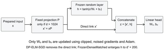
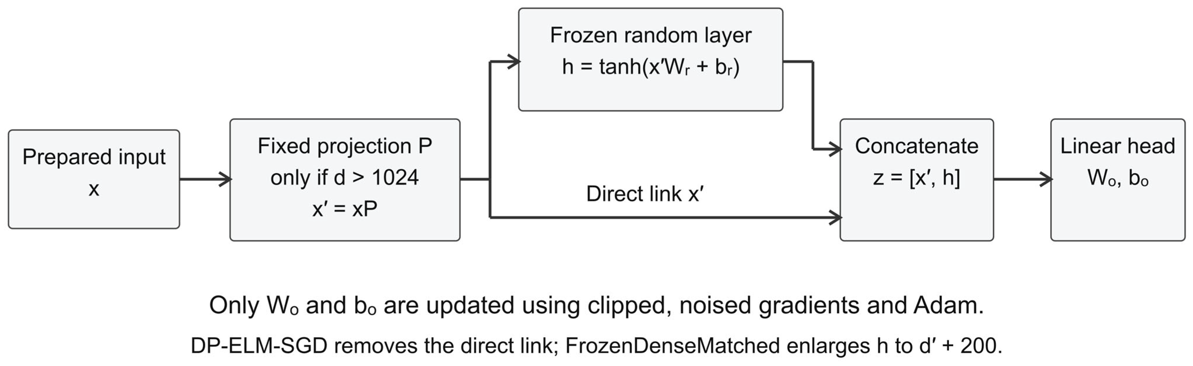
On CIFAR-10, the direct path carries x′, not all 3072 raw coordinates. Frozen layers are still evaluated during training and inference, and their stored weights are included in total parameter storage. Figure 1 separates the fixed representation from the privately optimized head.

Figure 1. DP-RVFL computation and the privately optimized parameter set. The Gaussian projection is used only when the input dimension exceeds 1024. The direct-link ablation removes x′ from the concatenation; the matched frozen control expands the hidden-only representation to d′ + 200 features. No feature cache is assumed in the timing measurements.

3.5. Controls and Published DP-ELM Implementation

DP-ELM-SGD uses the same projection, seed, 200 tanh hidden features, optimizer and privacy mechanism as DP-RVFL, but z = h. This isolates removal of the direct input path within the specified architecture, while also reducing the output dimension. It is not a reproduction of Ono et al.’s sufficient-statistic perturbation method.

FrozenDenseMatched uses the same input-reduction rule and a frozen tanh hidden layer of width d′ + 200, without a direct link. Its output head therefore has exactly the same number of trainable coefficients, K(d′ + 200 + 1), as RVFL for K output logits. K = 1 for binary gradient-trained models and K = 10 for the image models. The control matches the trainable head count, not the total frozen parameter count, feature values or computational cost. On the full-resolution CIFAR-10 input, the matched head has 12,250 trainable parameters.

LogisticRaw fits a single affine binary or multinomial classifier to the full prepared input. LogisticProjected uses the same data-independent projection as RVFL when the input dimension exceeds 1024 and has no nonlinear hidden features. On the other primary datasets, the two logistic representations coincide; their separate private runs need not return identical values because secure noise is independently drawn. All gradient-trained controls use the same settings in Section 3.2.

The numerical DP-ELM comparison follows Algorithm 1 of Ono et al. [11]. It forms sigmoid hidden features H, one-hot targets Y, the Gram matrix H^TH and the cross-product H^TY. Independent Laplace noise with scale L(L + 2)/ε is added to every entry of both matrices, and the noisy system is solved for the L × K output coefficients. No direct link, Gaussian projection, ridge term or symmetrization is applied. Widths L ∈ {1, 3, 5, 10} are all reported; no winning width is selected from validation or test results. These small widths provide a width-sensitivity comparison for the quadratic noise scale, not a parameter-matched comparison with the 200-feature gradient models.

The published algorithm specifies normal random weights and biases; our implementation explicitly uses N(0, 1), float64 arithmetic, a 1024-record accumulation chunk and a pseudoinverse fallback if the noisy solve is singular. The fallback operates only on the noised matrices. Sigmoid features lie in (0, 1), and each target is one-hot. For an added or removed record, the joint ℓ₁ contribution is bounded by L² + L, so the published conservative scale L(L + 2)/ε also covers this adjacency in ideal arithmetic. The published replace-one analysis and this conservative add/remove comparison are distinguished in the run metadata. The operating system-backed inverse-CDF Laplace implementation is not certified against finite-precision leakage; the pure-DP statement is the analytical ideal-mechanism guarantee, not a claim of an audited production sampler.

3.6. Algorithm and Auxiliary Experiments

Algorithm 1 describes one private gradient-training run. The public configuration is fixed before the run. Feature initialization is independent of training values, clipping and noise occur at every step, and the final checkpoint is used without validation selection. For the trained Dense/CNN baselines, the trainable set includes all network weights; for DP-RVFL and frozen-feature controls, it contains only the output head. The separate closed-form DP-ELM procedure in Section 3.5 does not execute this algorithm.

Algorithm 1. One fixed private gradient-training run

Input: prepared training records D; public N0, B, E, ε, δ and C; fixed model configuration and initialization seed. 1. Initialize the data-independent representation and output layer. Freeze P, Wr and br for DP-RVFL. Set θ to the trainable parameters. 2. Set J = ⌈N0/B⌉, q = 1/J, T = EJ and m0 = max(1, ⌊qN0⌋). Fix these values across neighboring inputs. 3. Calibrate σ using the RDP accountant for q, T, δ and target ε. Reject a calibration exceeding the target. 4. Initialize Adam and the secure private optimizer. Do not access the validation partition. 5. For t = 1, …, T, independently include each record with probability q to obtain Bt. 6. Compute per-example gradients for θ and clip their joint ℓ2 norm to C. If Bt is empty, use a zero clipped sum. 7. Add Gaussian noise with covariance σ2C2I to the clipped sum and divide by the fixed m0. 8. Update θ and Adam state using only this sanitized gradient. Record one accountant step, including empty-batch steps. 9. Verify that executed and accounted steps equal T and achieved ε is no greater than target ε. Output: the final fixed-epoch model and public protocol/accounting parameters. Do not release raw private diagnostics.

The image-sensitivity stage compares raw pixels in [0, 1], fixed centering/scaling (x − 0.5)/0.5, and half-resolution inputs of 14 × 14 for MNIST or 16 × 16 for CIFAR-10. The half-resolution profile uses torchvision.transforms.Resize followed by ToTensor. Each profile is fixed independently of training records, and none is selected as a final tuned preprocessing pipeline. Four Heart partition seeds, 2026–2029, assess split sensitivity while retaining five model seeds within each split.

A compact discriminative multi-head attention control uses 4 × 4 patches, 32-dimensional embeddings, four heads, fixed two-dimensional sinusoidal positions, one attention block, a 64-unit ReLU feed-forward sublayer, residual connections, mean token pooling and a linear classifier. The query/key/value and output projections are trainable. It uses neither layer normalization nor dropout and receives no pretraining. Multi-head attention is an architectural component [22]; this experiment is not a generative-AI evaluation or a benchmark of large pretrained transformers.

4. Experimental Results and Discussion

4.1. Datasets, Preprocessing and Experimental Configuration

The evaluation uses two image datasets and two structured cardiovascular datasets. The inclusion of both modalities supports an architecture-level analysis of whether the behavior observed under DP-SGD depends on the statistical and structural characteristics of the input data.

MNIST is a benchmark dataset containing grayscale images of handwritten digits from zero to nine [6]. Each image has a spatial resolution of 28 × 28 pixels and belongs to one of ten classes.

CIFAR-10 is a ten-class image dataset containing color images from categories such as vehicles and animals [7]. Each image has a resolution of 32 × 32 pixels and contains three color channels.

Their official test sets are retained. The supplied Cardio file contains 70,000 records from the Cardiovascular Disease dataset [23]; the supplied Heart file contains 303 records and is attributed to the Heart Disease Details distribution cited in [24]. Table 1 gives the actual prepared sample counts. These public files are benchmarks; no new patient cohort, prospective collection or hospital deployment is reported.

Table 1. Prepared primary benchmark partitions and input dimensions. Validation partitions are reserved but never accessed for fitting, tuning, threshold selection or checkpoint selection. Image dimensions precede any model-specific projection.

Dataset	Train	Unused Val.	Test	Prepared Input
MNIST	51,000	9000	10,000	1 × 28 × 28
CIFAR-10	42,500	7500	10,000	3 × 32 × 32
Cardio	48,025	10,291	10,292	32 features
Heart	212	45	46	47 features

Cardio preprocessing removes the identifier, converts age in days to years using division by 365.25, and derives BMI from weight and height. Public cohort filters retain height 120–220 cm, weight 30–200 kg, systolic pressure 80–250 and diastolic pressure 40–150, with systolic pressure at least diastolic pressure. The cleaned file contains 68,608 of 70,000 records. The recorded duplicate-removal count is zero. Heart retains all 303 records; the binary target is whether the target value is greater than zero. These are the implemented cleaning rules, not proposed clinical screening criteria.

Tabular numerical fields use fixed engineering bounds, clipping and a linear map to [−1, 1]. Missing or non-finite values are replaced by the midpoint of the specified bound and accompanied by a missingness indicator. Prespecified categorical values receive one-hot indicators and an additional unknown-category indicator. No mean, median, variance, category vocabulary or standard scaler is fitted to training records. This yields 32 Cardio features and 47 Heart features. Table S2 lists every bound and categorical set. Public cohort cleaning and source-file audit information remain outside the single-run training guarantee described in Section 3.1.

The image training sets are split 85%/15% into training and unused validation partitions. The tabular files are split 70%/15%/15% into training, unused validation and test partitions, using integer cut points of the permutation. No label stratification is used. The main image profile is ToTensor scaling to [0, 1], with no augmentation. A train-majority-class predictor has test accuracy 11.35% on MNIST, 10.00% on CIFAR-10, 50.30% on Cardio and 41.30% on Heart. The Heart test-set majority is instead 58.70%; the lower train-majority baseline results from the class-frequency reversal between its small training and test partitions.

The main design evaluates seven gradient-trained architectures and four closed-form ELM widths in private and non-private conditions, using model seeds 42–46. Private target budgets are ε ∈ {0.1, 0.5, 1, 2, 4, 8}. For all Gaussian mechanism runs,

δ = 10⁻⁵

(21)

The closed-form DP-ELM analytical mechanism uses δ = 0. The seven gradient models use ten epochs on images and thirty on tabular data; requested batch sizes are 256 except Heart, which uses 64. Table 2 distinguishes requested batch size from the fixed private normalizer. All use the final fixed-epoch checkpoint, constant learning rate, no early stopping and no hyperparameter search. Table S1 supplies the full model-by-dataset settings, including architecture, initialization, loss and dropout. Using common settings controls the experiment, but does not establish that every model is individually optimized.

Table 2. Primary Gaussian mechanism training schedule, held fixed across architectures within each dataset. B is the requested batch size, E the epoch count, q the Poisson inclusion probability, m₀ the fixed gradient normalizer and T the total updates. The realized batch size varies.

Dataset	B	E	q	m0	T
MNIST	256	10	0.00500000	255	2000
CIFAR-10	256	10	0.00598802	254	1670
Cardio	256	30	0.00531915	255	5640
Heart	64	30	0.25000000	53	120

Three complete executions each contain 2536 successful tasks: 1540 primary tasks, 360 diagnostic tasks, 360 image-profile tasks, 240 Heart split tasks and 36 attention tasks, giving 7608 completed tasks in total. Attention uses three model seeds, 42–44; the other stages use five, 42–46. Corresponding stages have identical recorded configurations, source-code hashes and prepared-data identities across executions. The first suite is retained as the primary analysis. Suites 2 and 3 are repeat executions and are reported separately, without pooling the repeated initialization seeds. The primary results use suite 1; the repeat-execution comparison summarizes all three executions.

The runs use CPU execution with eight PyTorch intra-op threads on the supplied Dell G15 5530 configuration, Intel Core i7-13650HX, 16 GB RAM, NVIDIA GeForce RTX 4060 Laptop GPU (8 GB) and Windows 11. The recorded environment includes Python 3.12.10, PyTorch 2.4.1, torchvision 0.19.1 and Opacus 1.5.4. Training times exclude privacy-engine setup and final test evaluation; setup-inclusive times are also reported for the CIFAR-10 comparison in Section 4.6. The diagnostic stage is kept separate because collecting per-example summaries adds work.

4.2. Metrics and Statistical Interpretation

Performance was evaluated using classification utility, privacy level, and computational cost. For MNIST and CIFAR-10, classification accuracy was used as the primary metric. Macro-averaged precision, recall, and F1-score were also calculated so that each class contributed equally to the reported result.

For Cardio and Heart, accuracy, precision, recall, F1-score, AUROC, and AUPRC were evaluated. AUROC measures the ability of a model to rank positive examples above negative examples across classification thresholds. AUPRC summarizes the relationship between precision and recall and is particularly informative when class distributions are imbalanced.

Classification accuracy is defined as

$$\begin{array}{c}\mathrm{Accuracy}={\displaystyle \frac{\mathit{TP}+\mathit{TN}}{\mathit{TP}+\mathit{TN}+\mathit{FP}+\mathit{FN}}},\end{array}$$

(22)

where TP, TN, FP, and FN denote the numbers of true positives, true negatives, false positives, and false negatives, respectively.

Precision is calculated as

$$\begin{array}{c}\mathrm{Precision}={\displaystyle \frac{\mathit{TP}}{\mathit{TP}+\mathit{FP}}},\end{array}$$

(23)

while recall is calculated as

$$\begin{array}{c}\mathrm{Recall}={\displaystyle \frac{\mathit{TP}}{\mathit{TP}+\mathit{FN}}}.\end{array}$$

(24)

The F1-score is the harmonic mean of precision and recall:

$$\begin{array}{c}\mathrm{F}1=2{\displaystyle \frac{\mathrm{Precision}\times \mathrm{Recall}}{\mathrm{Precision}+\mathrm{Recall}}}\end{array}$$

(25)

For multi-class tasks, precision, recall, and F1-score were calculated independently for each class and then macro-averaged.

Binary prediction uses the fixed probability threshold 0.5, and multiclass prediction uses argmax. AUROC is computed from class scores, using one-versus-rest macro averaging for multiclass tasks. The reported AUPRC uses average_precision_score, a recall-weighted average precision calculation rather than trapezoidal interpolation of the precision–recall curve.

To describe the utility preserved after private training, retained utility was calculated as

$$\begin{array}{c}\mathrm{Retained\; Utility}={\displaystyle \frac{{\mathrm{Accuracy}}_{\mathrm{private}}}{{\mathrm{Accuracy}}_{\mathrm{non}-\mathrm{private}}}}\times 100.\end{array}$$

(26)

This ratio is not a ranking criterion: a model with low non-private accuracy can have a high ratio while remaining less accurate in absolute terms. All comparative conclusions below identify the actual model, dataset and privacy condition.

Training time was measured in seconds and included the optimization procedures associated with each model. For private models, this included per-example gradient processing, gradient clipping, Gaussian-noise addition, and privacy accounting. Privacy-engine setup and final test evaluation are excluded from training-loop time and identified separately where reported.

Results are reported as mean ± sample standard deviation (SD) over training seeds. The numerical archive provided in the Supplementary Material also gives 95% Student-t intervals, with four degrees of freedom for five-seed experiments and two for attention. These intervals describe stochastic training variability conditional on the fixed public test partition. Estimating predictive uncertainty for a patient population requires evaluation on independent cohorts and an analysis that accounts for test-sample uncertainty. This requirement concerns predictive generalization; the stated per-run differential privacy guarantee is determined separately by the specified adjacency, sampling and privacy-accounting assumptions.

Paired contrasts align model seeds within each dataset–budget condition. Exact two-sided sign-flip tests enumerate the 2⁵ sign assignments for five differences. Their smallest attainable two-sided p-value is 0.0625, so this design cannot establish p < 0.05 even before multiplicity correction. Holm adjustment [25] is applied to all 960 reported primary contrasts within each suite, covering four datasets, six budgets, ten comparators and four metrics. All adjusted p-values are 1.0 in each of the three suites. Reusing the five initialization seeds and fixed public partitions does not create fifteen independent initialization seeds or independent test samples. Numerical differences and win counts are descriptive; absence of significance is not evidence of equivalence.

4.3. Non-Private Reference and Private Accuracy

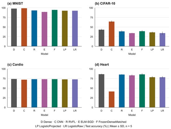
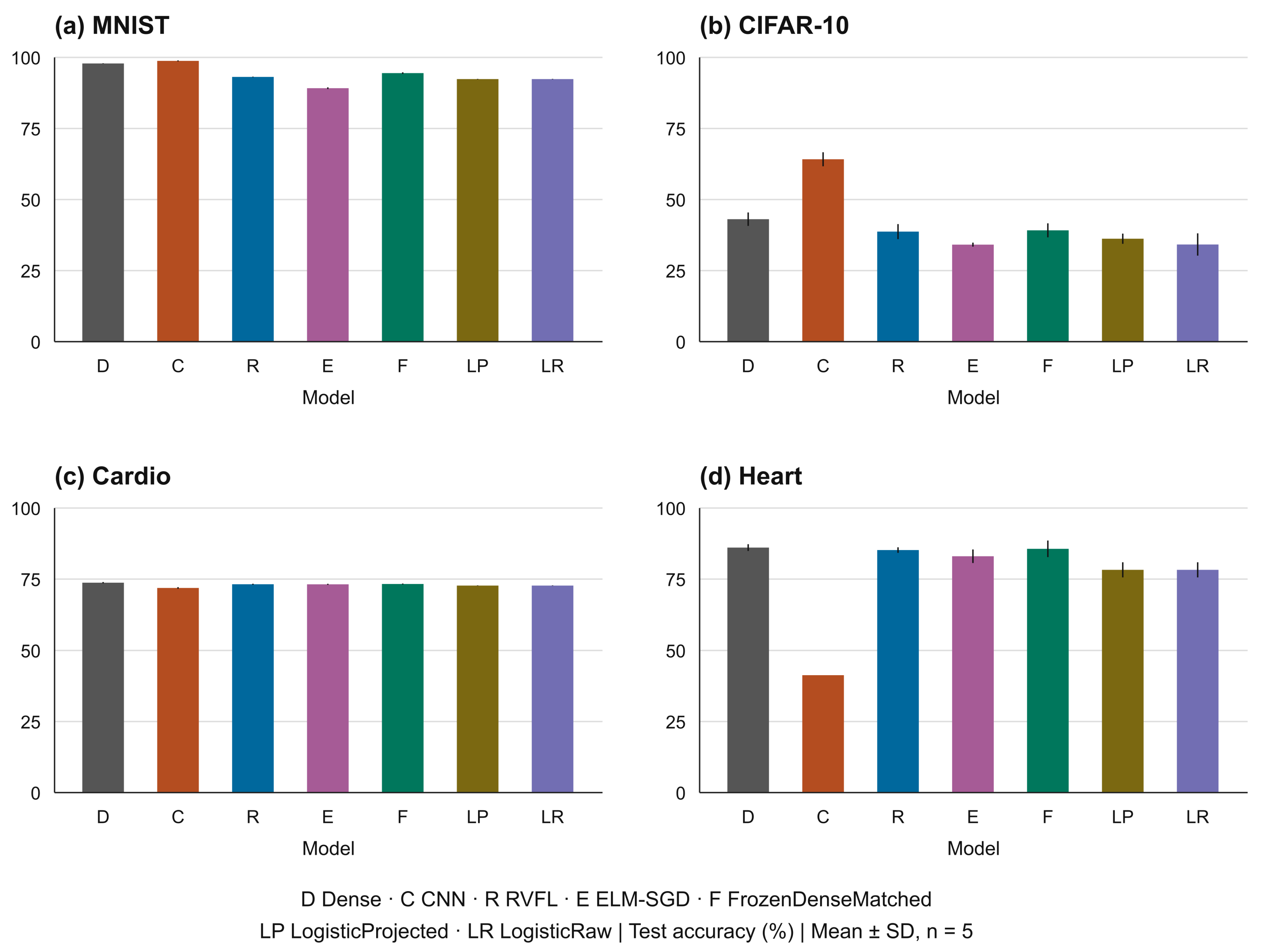
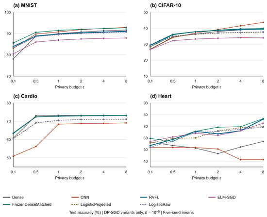
Figure 2 reports only non-private models. Figure 3 reports only the seven Gaussian mechanism variants across privacy budgets, and Table 3 gives their common ε = 2 slice. These are distinct conditions, not inconsistent estimates of the same configuration. Tables S4–S7 include every primary model, closed-form width and privacy budget with SDs. No model or width is selected separately for each table cell.

Figure 2. Non-private test accuracy for the seven gradient-trained architectures. Bars show five-seed means and error bars show SD. These runs have neither clipping nor DP noise. DPELM closed-form references are listed separately in Tables S4–S7. Different privacy conditions in Table 3 must not be compared as though they were the same experiment.

Figure 3. Test accuracy of the seven Gaussian mechanism architectures under add/remove-one adjacency and δ = 10⁻⁵. Points show five-seed means for each target ε; the equally spaced horizontal positions represent the six discrete tested budgets, not a linear ε scale. Panel vertical ranges differ. Tables S4–S7 give the corresponding SDs and non-private references; the numerical archive contains confidence intervals. Pure-DP DP-ELM is excluded from these curves because its mechanism and guarantee differ. Dashed curves denote LogisticProjected and LogisticRaw; solid curves denote the other five architectures.

Table 3. Private test accuracy (%) at ε = 2 and δ = 10⁻⁵ in the primary suite, mean ± SD over five seeds. Every row uses the Gaussian gradient mechanism; FrozenDenseMatched matches the RVFL trainable head count. Higher numerical means are not claims of statistical superiority.

Private Model	MNIST	CIFAR-10	Cardio	Heart
Dense	90.69 ± 0.17	37.93 ± 0.34	73.14 ± 0.04	46.52 ± 4.76
CNN	91.80 ± 0.33	39.13 ± 0.89	68.73 ± 0.18	50.43 ± 8.75
RVFL	90.30 ± 0.16	38.61 ± 0.24	72.99 ± 0.20	63.48 ± 12.43
ELM-SGD	87.43 ± 0.29	33.72 ± 0.65	72.92 ± 0.16	62.17 ± 8.64
FrozenDenseMatched	91.96 ± 0.11	38.83 ± 0.45	72.96 ± 0.19	69.13 ± 11.02
LogisticProjected	90.04 ± 0.12	36.93 ± 0.35	70.93 ± 0.19	66.09 ± 6.26
LogisticRaw	90.06 ± 0.08	37.06 ± 0.39	70.98 ± 0.19	65.65 ± 7.28

On MNIST at ε = 2, DP-RVFL obtains 90.30 ± 0.16%, compared with 87.43 ± 0.29% for DP-ELM-SGD, 91.96 ± 0.11% for DP-FrozenDenseMatched and 91.80 ± 0.33% for DP-CNN. The direct-link model exceeds the hidden-only 200-feature ablation in this condition, but not the larger matched frozen representation. At ε = 0.1 its accuracy is 83.91%, compared with 83.04% for DP-CNN and 85.58% for the matched frozen control. At ε = 8, DP-RVFL reaches 91.02% and DP-CNN 92.88%.

On CIFAR-10 at ε = 2, DP-RVFL obtains 38.61 ± 0.24%, DP-ELM-SGD 33.72 ± 0.65%, DP-FrozenDenseMatched 38.83 ± 0.45% and DP-CNN 39.13 ± 0.89%. At ε = 8, DP-RVFL reaches 39.40% and DP-CNN 43.62%. The non-private CNN reaches 64.17%, while non-private RVFL reaches 38.72%. Thus, the high retained-utility ratio of RVFL on this dataset partly reflects its lower non-private reference. It does not establish that its representation is preferable for unconstrained image classification. For this RVFL configuration, the non-private and private results at ε = 2 indicate that low absolute accuracy is not primarily explained by privacy noise at that budget. By contrast, the CNN decreases from 64.17% without privacy to 39.13% at ε = 2 under the combined clipping-and-noise protocol. These comparisons do not isolate the causal contributions of representation, preprocessing and optimization settings.

Across the 24 primary dataset–budget conditions, DP-RVFL has higher mean accuracy than DP-ELM-SGD in 20 conditions, ties in one and is lower in three. Against DP-FrozenDenseMatched, the counts are eight higher, one tied and fifteen lower. It is higher than DP-LogisticProjected in 20 conditions and higher than DP-CNN in sixteen. These counts describe this fixed protocol and do not isolate a single causal mechanism. In particular, removal of the direct link changes representation dimension, and equal trainable parameter counts do not imply equal feature quality or optimization behavior.

4.4. Tabular Outcomes and Low-Budget Uncertainty

At ε = 2, Cardio accuracy is 72.99 ± 0.20% for DP-RVFL, 73.14 ± 0.04% for DP-Dense, 72.92 ± 0.16% for DP-ELM-SGD and 72.96 ± 0.19% for DP-FrozenDenseMatched. The difference between DP-RVFL and the no-link ablation is small numerically in this condition. Table 4 reports F1 and ranking metrics alongside accuracy so that conclusions do not depend on a single score or threshold.

Table 4. DP-RVFL predictive metrics at ε = 0.1 and ε = 2 in the primary suite, mean ± SD over five seeds. Metrics are on the 0–1 scale. Image F1, AUROC and average precision are macro-averaged; binary results use the positive class. AUPRC denotes the implementation’s average precision.

Dataset/ε	Accuracy	F1	AUROC	AUPRC
MNIST/0.1	0.839 ± 0.003	0.835 ± 0.003	0.983 ± 0.000	0.916 ± 0.002
MNIST/2	0.903 ± 0.002	0.901 ± 0.002	0.992 ± 0.000	0.958 ± 0.001
CIFAR-10/0.1	0.293 ± 0.005	0.281 ± 0.003	0.737 ± 0.004	0.266 ± 0.005
CIFAR-10/2	0.386 ± 0.002	0.375 ± 0.005	0.804 ± 0.001	0.377 ± 0.003
Cardio/0.1	0.635 ± 0.015	0.545 ± 0.029	0.756 ± 0.004	0.730 ± 0.004
Cardio/2	0.730 ± 0.002	0.704 ± 0.005	0.792 ± 0.001	0.775 ± 0.001
Heart/0.1	0.535 ± 0.127	0.441 ± 0.270	0.597 ± 0.167	0.702 ± 0.128
Heart/2	0.635 ± 0.124	0.543 ± 0.243	0.884 ± 0.027	0.909 ± 0.031

At ε = 0.1, Cardio DP-RVFL accuracy is 63.51%, with a training-seed 95% interval of 61.63–65.38%, compared with the 50.30% train-majority baseline. The matched frozen model has a mean accuracy of 63.25%. Heart DP-RVFL accuracy is 53.48%, with SD 12.73 percentage points and a 95% interval of 37.67–69.29%; its matched frozen comparator reaches 59.57%. A single Heart test error changes accuracy by 2.17 percentage points because the test partition contains only 46 records. These findings do not support a general claim that DP-RVFL reliably preserves tabular utility at the strictest budget.

At a fixed sampling rate, update count and δ, a smaller target ε requires a larger calibrated Gaussian-noise multiplier. This stricter privacy constraint can hinder optimization; low accuracy itself is not a measure of security. Heart’s small training partition and 46-record test partition also limit the precision and stability of the observed scores. Each of the four datasets was trained and evaluated separately, without pooling image and medical records. The reported experiments do not identify dataset origin or collection quality as a causal explanation for the accuracy differences.

For Heart at ε = 2, DP-RVFL accuracy is 63.48 ± 12.43% and F1 is 0.543 ± 0.243, although its mean AUROC is 0.884. Ranking discrimination and classification at a fixed threshold are different properties. No test-based threshold adjustment was applied to raise accuracy or F1. Neither the AUROC nor the resampling analysis below establishes clinical calibration, decision benefit or external validity.

Accuracy, F1, AUROC and average precision are quantitative measures of classification performance. They evaluate binary disease labels, although several predictors, such as age and blood pressure, are continuous measurements. Input-data quality is a separate property, involving measurement units, plausible ranges, missingness, label reliability and coverage of the intended population. In Cardio, the recorded cohort rules reduced 70,000 rows to 68,608; the fixed-bound encoding then handled numerical and categorical inputs as described in Section 4.1. These steps document preprocessing, but do not independently verify label accuracy or population representativeness.

A clinical assessment should report calibration and decision consequences at prespecified thresholds alongside discrimination, and evaluate an independent intended-use cohort, consistent with the distinctions in TRIPOD + AI [26]. These analyses would assess whether numerical predictions support the intended clinical decision; they were not performed in this benchmark comparison.

4.5. Comparison with Published DP-ELM

Table 5 reports all four prespecified DP-ELM widths at ε = 2. For L = 10, mean accuracies are 38.17% on MNIST, 17.39% on CIFAR-10, 58.61% on Cardio and 41.30% on Heart. These are results of the specified numerical reproduction with sigmoid features, normal initialization and no regularization. They should not be generalized to every ELM configuration or described as an isolated effect of the RVFL direct link.

Table 5. Numerical DP-ELM test accuracy (%) at ε = 2 for each fixed width, mean ± SD over five seeds. The cited method’s analytical mechanism is pure DP (δ = 0); finite-precision certification is not claimed. These values are not an equal-guarantee, equal-width or equal-loss comparison with Table 3. Corresponding non-private closed-form results and all six budgets appear in Tables S4–S7.

Width L	MNIST	CIFAR-10	Cardio	Heart
1	10.08 ± 0.16	10.20 ± 0.23	49.82 ± 0.27	48.26 ± 9.53
3	18.47 ± 1.80	12.53 ± 1.10	53.30 ± 2.88	59.57 ± 9.79
5	25.26 ± 1.44	15.29 ± 1.83	58.75 ± 3.59	51.74 ± 16.66
10	38.17 ± 2.56	17.39 ± 2.17	58.61 ± 5.42	41.30 ± 13.40

The perturbation scale is 60 at L = 10 and ε = 2, and 1200 at L = 10 and ε = 0.1. Increasing hidden width changes both representation capacity and the noise applied to the sufficient statistics. The Heart L = 10 results at ε = 2 are 41.30%, 50.43% and 44.35% in suites 1, 2 and 3, respectively, which cautions against selecting a favorable realization. The same-mechanism no-link results in Section 4.3 provide a more targeted assessment of the direct path. The low DP-ELM scores must therefore be interpreted under both the restricted hidden widths and the width-dependent perturbation, rather than attributed solely to the absence of a direct input link.

4.6. Training Time and Computational Quantities

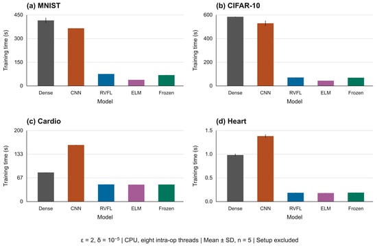
Figure 4 reports training-loop time at ε = 2. On MNIST, DP-RVFL takes 75.95 s, DP-CNN 365.52 s and DP-Dense 415.46 s. On CIFAR-10, the corresponding values are 71.29 s, 529.76 s and 584.58 s, giving measured training time ratios of 7.43 for CNN/RVFL and 8.20 for Dense/RVFL. These ratios apply to this CPU execution and schedule. They are not inference speedups or scaling-law estimates.

Figure 4. Private training-loop time at ε = 2 and δ = 10⁻⁵. Bars are five-seed means and error bars are SD. The datasets have different training sizes and epoch counts. All runs use eight CPU intra-op threads; privacy-engine setup and final test evaluation are excluded. Diagnostic runs are not used for these timing comparisons.

Fewer trainable parameters do not imply smaller total storage or fewer forward operations (Table 6). CIFAR-10 DP-RVFL has 12,250 trainable parameters, but its fixed projection and random layer contribute to 13,451,912 stored bytes. DP-CNN has 545,098 trainable parameters and 2,180,392 stored bytes. Estimated forward MACs are 3,362,768 for RVFL and 6,128,896 for CNN; Dense requires 820,480 despite its longer measured private training time. Gradient processing, backward computation, memory traffic and data loading are excluded from forward MAC estimates and affect runtime. Calibration is cached for identical public accounting configurations, so setup-inclusive times reflect this execution order and are not independent cold-start measurements.

Table 6. CIFAR-10 resource quantities at ε = 2. Times are five-seed means in seconds; setup-inclusive time adds privacy-engine construction and calibration. MACs are estimated forward multiply–accumulate operations per record, and MiB denotes 2²⁰ stored parameter bytes. Storage includes frozen parameters and model buffers where counted but excludes optimizer states and activations. These estimates are not peak-memory measurements or total training FLOPs.

Model	Trainable	Train s	Setup + Train s	MACs (M)	MiB
Dense	820,874	584.58	585.08	0.820	3.131
CNN	545,098	529.76	529.76	6.129	2.079
RVFL	12,250	71.29	71.29	3.363	12.829
ELM-SGD	2010	44.52	44.52	3.353	12.790
FrozenDenseMatched	12,250	69.67	69.68	4.411	16.833
LogisticProjected	10,250	62.22	62.22	3.156	12.039
LogisticRaw	30,730	95.22	95.23	0.031	0.117

The no-link CIFAR-10 model takes 44.52 s and FrozenDenseMatched takes 69.67 s, compared with 71.29 s for RVFL. Thus, the runtime advantage is relative to the tested fully trained Dense/CNN models, not to every frozen-feature alternative. For unprojected dimension d, reduced dimension d′, hidden width L and output size K, RVFL forward work scales as O(dd′ + d′L + (d′ + L)K) when a dense projection is required; the dd′ term is omitted otherwise. Stored coefficients include that projection and random map, whereas only (d′ + L + 1)K coefficients require gradient updates. This distinction explains why trainable parameter count alone is an incomplete resource measure.

4.7. Clipping and Image-Preprocessing Sensitivity

The separate diagnostic stage measures pre-clipping per-example gradient norms, loss and clipping frequency on public records. At ε = 2 on CIFAR-10, the fraction of sampled records clipped, weighted by record draws across epochs and then averaged over seeds, is 99.92% for DP-RVFL, 99.92% for DP-ELM-SGD, 99.18% for DP-FrozenDenseMatched and 99.97% for DP-CNN. These fractions do not support the earlier explanation that DP-RVFL’s accuracy is due to substantially less clipping. With fixed q, T, C and δ, the calibrated multiplier is the same across these architectures. The parameter dimension changes the noise vector, but the measured comparisons do not establish how much of a utility difference is caused by dimension, representation or optimization. The third execution gives clipping fractions of 99.92% for DP-RVFL and 99.17% for DP-FrozenDenseMatched under the same condition; this repeat does not change the interpretation (Table S10).

For CIFAR-10, DP-CNN accuracy changes from 40.12% under raw01 to 46.15% under fixed centering and 36.67% at half resolution (Table 7). DP-RVFL changes from 38.54% to 39.27% and 38.12%, respectively. Under non-private training, the corresponding CNN values are 64.17%, 68.07% and 54.78%. The results show sensitivity to the tested preprocessing configurations; they do not identify poor resolution as the sole explanation of the original accuracy. Downsampling also changes model input dimensions and whether projection is needed. No medical/image data mixture is involved, and lower accuracy is not evidence of stronger privacy. In suite 3, the corresponding private CNN values are 39.39%, 45.98% and 36.64%, and the DP-RVFL values are 38.83%, 39.51% and 38.24% (Table S10). The repeated comparison retains the observed dependence on preprocessing within these configurations.

Table 7. Image-profile sensitivity at ε = 2 and δ = 10⁻⁵, mean ± SD accuracy (%) over five seeds in the separate image stage. The raw01 profile is full-resolution [0, 1] input; fixed-centered uses (x − 0.5)/0.5 at full resolution; half-resolution uses [0, 1] inputs at 14 × 14 for MNIST or 16 × 16 for CIFAR-10. Secure private runs in this stage are distinct from those in Table 3.

Dataset	Profile	DP-RVFL	DP-CNN
MNIST	raw01	90.32 ± 0.11	91.67 ± 0.16
MNIST	fixed centered	90.53 ± 0.19	93.84 ± 0.85
MNIST	half resolution	90.66 ± 0.32	88.30 ± 1.48
CIFAR-10	raw01	38.54 ± 0.45	40.12 ± 0.95
CIFAR-10	fixed centered	39.27 ± 0.43	46.15 ± 0.54
CIFAR-10	half resolution	38.12 ± 0.18	36.67 ± 0.69

4.8. Heart Partition Sensitivity and the Attention Control

Table 8 reports each Heart split separately. DP-RVFL mean accuracy at ε = 2 is 63.04%, 73.04%, 90.43% and 68.70% for split seeds 2026, 2027, 2028 and 2029. The split-2026 result is a separate secure-noise realization from the primary run. These estimates average training seeds within each partition; they are not pooled as twenty independent patients or twenty independent datasets. In suite 3, the corresponding split means are 65.22%, 71.74%, 90.00% and 68.26% (Table S10), retaining sensitivity to partition choice within the same small cohort.

Table 8. Heart partition-sensitivity accuracy (%) at ε = 2 and δ = 10⁻⁵, mean ± SD over five model seeds within each split. Each split contains 212 training, 45 unused validation and 46 test records drawn from the same 303-record public file. The partitions overlap and are not external cohorts.

Split Seed	DP-RVFL	DP-ELM-SGD	DP-FrozenDenseMatched	DP-LogisticRaw
2026	63.04 ± 12.10	59.57 ± 9.43	66.09 ± 5.46	66.09 ± 6.26
2027	73.04 ± 10.49	69.13 ± 9.40	74.78 ± 12.45	69.57 ± 7.37
2028	90.43 ± 3.30	82.17 ± 11.65	88.26 ± 3.30	79.57 ± 6.26
2029	68.70 ± 6.45	68.70 ± 5.87	71.30 ± 2.83	64.35 ± 4.76

The wide range of split means limits claims based on the original Heart partition. Changing the split does not provide new clinical validation or establish that any favorable partition represents a target population. An external cohort, prespecified endpoints and a deployment-specific assessment would be required for a clinical claim.

The private attention control reaches 29.12% on MNIST and 25.70% on CIFAR-10, compared with 90.26% and 38.57% for DP-RVFL in the same stage (Table 9). These results do not establish that attention is generally unsuitable for private learning. They describe one small architecture without pretraining, normalization or model-specific tuning. Large pretrained or augmented image models are not evaluated under a matched compute budget, so no state-of-the-art ranking is claimed. The third execution gives 29.83% on MNIST and 26.66% on CIFAR-10 for the attention control (Table S10), using the same three initialization seeds; the repeated runs do not broaden the architectural or application scope.

Table 9. Compact attention-control results, mean ± SD accuracy (%) over three seeds in the separate attention stage. Private results use ε = 2 and δ = 10⁻⁵. The three architectures share the image-stage training schedule but have different capacities. Attention is discriminative, unpretrained and not individually tuned.

Dataset	Architecture	Non-Private	Private ε = 2
MNIST	RVFL	93.12 ± 0.09	90.26 ± 0.21
MNIST	CNN	98.71 ± 0.14	91.59 ± 0.02
MNIST	Attention	80.73 ± 0.71	29.12 ± 1.95
CIFAR-10	RVFL	38.62 ± 3.40	38.57 ± 0.44
CIFAR-10	CNN	65.55 ± 1.32	40.28 ± 1.07
CIFAR-10	Attention	43.92 ± 0.39	25.70 ± 3.11

4.9. Repeat Execution and Limitations

The second and third executions each complete all 2536 planned tasks with the same recorded protocol identities, configurations and public partitions as the primary suite. Table 10 reports DP-RVFL accuracy at ε = 2 across the three executions. MNIST means range from 90.26% to 90.30%, CIFAR-10 from 38.41% to 38.61%, and Cardio from 72.79% to 72.99%. Heart means range from 62.17% to 63.48%, while within-execution SDs range from 10.15 to 12.43 percentage points. Similar execution means therefore do not remove the substantial Heart training variability. All 220 non-private primary accuracy values match across executions; private outcomes vary with secure randomness that is not fixed by the public initialization seeds. Table S8 reports all primary models at ε = 2 for each execution. These repeated configurations are not treated as fifteen independent initialization seeds or as additional test populations.

Table 10. DP-RVFL accuracy (%) at ε = 2 and δ = 10⁻⁵ in the primary stage of each execution, mean ± SD over the same five model seeds. All three executions reuse the same public training and test partitions. Private randomness varies between executions. SD measures training variation within each execution; the results are not pooled.

Dataset	Suite 1	Suite 2	Suite 3
MNIST	90.30 ± 0.16	90.26 ± 0.08	90.26 ± 0.11
CIFAR-10	38.61 ± 0.24	38.41 ± 0.22	38.54 ± 0.21
Cardio	72.99 ± 0.20	72.99 ± 0.17	72.79 ± 0.18
Heart	63.48 ± 12.43	62.17 ± 10.15	62.61 ± 11.75

DP-RVFL has higher mean accuracy than DP-ELM-SGD in 20, 22 and 19 of the 24 dataset–budget conditions in suites 1, 2 and 3, respectively; the corresponding counts against DP-FrozenDenseMatched are eight, five and three (Table S9). In suite 3, DP-RVFL is lower than the matched frozen control in twenty conditions and tied in one. Condition-level rankings can change without reversing the absence of a general advantage over the matched frozen representation. All 960 primary Holm-adjusted p-values remain 1.0 in each execution. The repeated seed and cohort structure is retained in the reporting, rather than used to inflate the nominal number of independent comparisons.

At ε = 2 on CIFAR-10, DP-RVFL training times are 71.29, 70.83 and 71.88 s across the three executions, compared with 529.76, 518.46 and 534.12 s for DP-CNN and 44.52, 44.66 and 44.52 s for DP-ELM-SGD. The observed timing relationship persists for these configurations, including the faster no-link alternative. Table S10 reports the repeated timing and diagnostic results. The repeats assess execution variability under the same recorded environment and public records; they do not establish hardware scaling or population transportability.

The fixed random map has a representational cost: it cannot learn task-specific hidden features, and the tanh activation may compress distinctions in the projected inputs. Projection can discard information; larger hidden layers require storage and forward computation even when frozen. A direct input path expands the output layer and does not automatically improve its private optimization. Our ablations quantify outcomes for selected configurations but do not isolate all of these factors or measure activation saturation directly.

The experiments are limited to public benchmarks, small fixed architectures and common, prespecified hyperparameters. They do not measure external clinical utility, demographic subgroup performance, calibrated treatment decisions, poisoning resistance or deployed attack success. The public data are not synthetically generated by this study; nevertheless, the absence of synthetic generation does not establish representativeness. The independent training-record privacy mechanism, population generalization and application security are separate questions. The frozen-feature architecture does not remove the need for a complete privacy analysis of confidential cohort construction, tuning, evaluation and multiple releases. Finite-precision certification of the Laplace DP-ELM sampler also remains outside the implemented evaluation.

The medical tasks evaluated here are static binary classifications. Neither tabular file is analyzed as a timestamped series of repeated observations, and the one-dimensional tabular CNN does not model patient trajectories. A longitudinal extension would require time-indexed measurements, a defined prediction horizon and patient-separated, time-aware evaluation.

One follow-up study could compare a fixed temporal feature map and privately trained output head with recurrent or attention-based controls under matched privacy and compute budgets. This would test whether a frozen temporal representation retains useful trajectory information while reducing optimization cost. Privacy accounting would need to protect the complete patient trajectory when that is the intended privacy unit and account for repeated releases; the present record-level guarantee cannot be relabeled as patient-level privacy [4]. Independent clinical cohorts, calibration and threshold-specific decision analysis would be required to assess clinical use [26].

5. Conclusions and Future Work

Differentially private neural-network training requires balancing record-level privacy, predictive utility and computational cost. Gradient clipping and noise can reduce predictive performance, while privately optimizing a fully trainable network adds computational overhead. This study evaluated DP-RVFL as an approach that freezes a data-independent randomized hidden representation, retains a direct input-to-output connection and privately trains only the output head. Comparisons across image and cardiovascular tabular benchmarks examined whether this restricted optimization could reduce training time while maintaining predictive utility under the specified privacy budgets.

The principal observed advantage was lower CPU training-loop time relative to the tested fully trained Dense and CNN models. On CIFAR-10 at ε = 2 and δ = 10⁻⁵, DP-RVFL achieved 38.61% accuracy in 71.29 s, compared with 39.13% in 529.76 s for DP-CNN, yielding a 7.43-fold CNN/RVFL training time ratio under the same eight-thread setting. The corresponding Dense/RVFL ratio was 8.20. These measurements apply to the specified Poisson-sampled Gaussian gradient protocol and training schedules, exclude privacy-engine setup and final test evaluation, and do not establish equivalent predictive accuracy or faster inference.

The utility comparisons also define the limits of this computational advantage. DP-RVFL achieved higher mean accuracy than the corresponding 200-feature no-direct-link ablation in 20 of 24 primary conditions. However, the trainable-parameter-matched frozen control achieved higher mean accuracy in fifteen conditions, and the five-seed tests did not establish statistical superiority. Reducing the number of trainable parameters therefore did not produce a general accuracy advantage. Two repeated suites retained the observed timing relationship and the absence of a general accuracy advantage over the matched frozen control, but did not add independent initialization seeds or external test cohorts.

Future work should address the limitations identified by these comparisons. CIFAR-10 performance indicates a representational limitation relative to the non-private CNN, while Heart outcomes vary across small, overlapping partitions. Gradient diagnostics do not support an explanation based on substantially reduced clipping. Further evaluation should therefore include independently tuned controls under an explicitly budgeted selection procedure, larger and external tabular cohorts, and matched-compute comparisons with stronger private image models. Application to confidential data would additionally require a privacy analysis covering data preparation, model selection, evaluation and all released models.

References

- Bai, L.; Hu, H.; Ye, Q.; Li, H.; Wang, L.; Xu, J. Membership Inference Attacks and Defenses in Federated Learning: A Survey. ACM Comput. Surv. 2024, 57, 89. [Google Scholar] [CrossRef] [Scilit]
- Carlini, N.; Tramèr, F.; Wallace, E.; Jagielski, M.; Herbert-Voss, A.; Lee, K.; Roberts, A.; Brown, T.; Song, D.; Erlingsson, Ú.; et al. Extracting Training Data from Large Language Models. In Proceedings of the 30th USENIX Security Symposium (USENIX Security 21); USENIX Association: Berkeley, CA, USA, 2021; pp. 2633–2650. Available online: https://www.usenix.org/conference/usenixsecurity21/presentation/carlini-extracting (accessed on 1 October 2026).
- Dwork, C.; McSherry, F.; Nissim, K.; Smith, A. Calibrating Noise to Sensitivity in Private Data Analysis. In Proceedings of the Theory of Cryptography Conference; Springer: Berlin/Heidelberg, Germany, 2006; pp. 265–284. [Google Scholar] [CrossRef] [Scilit]
- Dwork, C.; Roth, A. The algorithmic foundations of differential privacy. Found. Trends Theor. Comput. Sci. 2014, 9, 211–407. [Google Scholar] [CrossRef] [Scilit]
- Abadi, M.; Chu, A.; Goodfellow, I.; McMahan, H.B.; Mironov, I.; Talwar, K.; Zhang, L. Deep learning with differential privacy. In Proceedings of the ACM Conference on Computer and Communications Security; Association for Computing Machinery: New York, NY, USA, 2016; pp. 308–318. [Google Scholar] [CrossRef] [Scilit]
- Deng, L. The MNIST Database of Handwritten Digit Images for Machine Learning Research [Best of the Web]. IEEE Signal Process. Mag. 2012, 29, 141–142. [Google Scholar] [CrossRef] [Scilit]
- Krizhevsky, A. Learning Multiple Layers of Features from Tiny Images; University of Toronto: Toronto, ON, Canada, 2009. [Google Scholar]
- Igelnik, B.; Pao, Y.-H. Stochastic Choice of Basis Functions in Adaptive Function Approximation and the Functional-Link Net. IEEE Trans. Neural Netw. 1995, 6, 1320–1329. [Google Scholar] [CrossRef] [Scilit] [PubMed]
- Sun, F.; Toh, K.-A.; Romay, M.G.; Mao, K. (Eds.) Extreme Learning Machines 2013: Algorithms and Applications; Springer: Cham, Switzerland, 2014. [Google Scholar] [CrossRef] [Scilit]
- Malik, A.K.; Gao, R.; Ganaie, M.A.; Tanveer, M.; Suganthan, P.N. Random vector functional link network: Recent developments, applications, and future directions. Appl. Soft Comput. 2023, 143, 110377. [Google Scholar] [CrossRef] [Scilit]
- Ono, H.; Phuong, T.T.; Phong, L.T. Differentially Private Extreme Learning Machine. In Modeling Decisions for Artificial Intelligence; Torra, V., Narukawa, Y., Kikuchi, H., Eds.; Springer Nature: Cham, Switzerland, 2024; pp. 165–176. [Google Scholar]
- Mironov, I. Rényi Differential Privacy. In Proceedings of the IEEE Computer Security Foundations Symposium; IEEE Computer Society: New York, NY, USA, 2017; pp. 263–275. [Google Scholar] [CrossRef] [Scilit]
- Mironov, I.; Talwar, K.; Zhang, L. Rényi Differential Privacy of the Sampled Gaussian Mechanism. arXiv 2019, arXiv:1908.10530. [Google Scholar] [CrossRef] [Scilit]
- Yousefpour, A.; Shilov, I.; Sablayrolles, A.; Testuggine, D.; Prasad, K.; Malek, M.; Nguyen, J.; Ghosh, S.; Bharadwaj, A.; Zhao, J.; et al. Opacus: User-Friendly Differential Privacy Library in PyTorch. arXiv 2022, arXiv:2109.12298. [Google Scholar] [CrossRef] [Scilit]
- Chaudhuri, K.; Monteleoni, C.; Sarwate, A.D. Differentially Private Empirical Risk Minimization. arXiv 2011, arXiv:0912.0071. [Google Scholar] [CrossRef] [Scilit]
- Giddens, S.; Zhou, Y.; Krull, K.R.; Brinkman, T.M.; Song, P.X.K.; Liu, F. A Differentially Private Weighted Empirical Risk Minimization Procedure and Its Application to Outcome Weighted Learning. IEEE Trans. Inf. Forensics Secur. 2026, 21, 6247–6257. [Google Scholar] [CrossRef] [Scilit]
- Huang, G.B.; Zhu, Q.Y.; Siew, C.K. Extreme learning machine: Theory and applications. Neurocomputing 2006, 70, 489–501. [Google Scholar] [CrossRef] [Scilit]
- Nowroozi, E.; Mohammadi, M.; Rahdari, A.; Taheri, R.; Conti, M. A Random Deep Feature Selection Approach to Mitigate Transferable Adversarial Attacks. IEEE Trans. Netw. Serv. Manag. 2025, 22, 5301–5310. [Google Scholar] [CrossRef] [Scilit]
- De, S.; Berrada, L.; Hayes, J.; Smith, S.L.; Balle, B. Unlocking High-Accuracy Differentially Private Image Classification Through Scale. arXiv 2022, arXiv:2204.13650. [Google Scholar] [CrossRef] [Scilit]
- Ziller, A.; Usynin, D.; Braren, R.; Makowski, M.; Rueckert, D.; Kaissis, G. Medical imaging deep learning with differential privacy. Sci. Rep. 2021, 11, 13524. [Google Scholar] [CrossRef] [Scilit] [PubMed]
- Kingma, D.P.; Ba, J. Adam: A Method for Stochastic Optimization. In Proceedings of the 3rd International Conference on Learning Representations, ICLR 2015, San Diego, CA, USA, 7–9 May 2015; Available online: http://arxiv.org/abs/1412.6980 (accessed on 1 October 2026).
- Vaswani, A.; Shazeer, B.; Parmar, N.; Uszkoreit, N.; Jones, V.; Gomez, A.N.; Kaiser, L.; Polosukhin, L. Attention Is All You Need. In Proceedings of the Advances in Neural Information Processing Systems; NeurIPS: San Diego, CA, USA, 2017; Volume 30. [Google Scholar]
- Ulianova, S. Cardiovascular Disease Dataset. Available online: https://www.kaggle.com/datasets/sulianova/cardiovascular-disease-dataset (accessed on 1 October 2026).
- Shakya, P. Heart Disease Details. Available online: https://www.kaggle.com/datasets/pratikshakya/heart-disease-details (accessed on 1 October 2026).
- Haynes, W. Holm’s Method. In Encyclopedia of Systems Biology; Dubitzky, W., Wolkenhauer, O., Cho, K.-H., Yokota, H., Eds.; Springer: New York, NY, USA, 2013; p. 902. [Google Scholar] [CrossRef] [Scilit]
- Collins, G.S.; Moons, K.G.M.; Dhiman, P.; Riley, R.D.; Beam, A.L.; Van Calster, B.; Ghassemi, M.; Liu, X.; Reitsma, J.B.; van Smeden, M.; et al. TRIPOD+AI statement: Updated guidance for reporting clinical prediction models that use regression or machine learning methods. BMJ 2024, 385, e078378. [Google Scholar] [CrossRef] [Scilit] [PubMed]
Disclaimer/Publisher’s Note: The statements, opinions and data contained in all publications are solely those of the individual author(s) and contributor(s) and not of MDPI and/or the editor(s). MDPI and/or the editor(s) disclaim responsibility for any injury to people or property resulting from any ideas, methods, instructions or products referred to in the content. |
© 2026 by the authors. Licensee MDPI, Basel, Switzerland. This article is an open access article distributed under the terms and conditions of the Creative Commons Attribution (CC BY) license.