


Abstract
In coastal wetlands, Tamarix chinensis often occurs as patches intermixed with Phragmites australis, Suaeda salsa, and saline–alkaline bare soil. This mixed distribution makes tamarisk prone to omission in medium-resolution remote sensing classification, while the recall of the target species is often masked by a relatively high overall accuracy. In this study, we focused on the Yellow River Delta National Nature Reserve and developed a multi-source feature set using summer 2025 Sentinel-2, Sentinel-1, and UAV/GPS data, comprising spectral, SAR, phenological, and red-edge-oriented features. To enhance the separability between tamarisk and co-occurring herbaceous vegetation, we introduced a red-edge–vegetation-cover coupling feature (REcov) based on their contrasting responses in the red-edge region. Within an XGBoost framework, we evaluated the marginal contribution of this feature using feature ablation, replacement, and spatial block cross-validation. The full feature set achieved an AUC of 0.8042, a recall of 0.9340, and an overall accuracy of 0.8194 on an independent test set. Ablation and replacement experiments showed that the red-edge-oriented features contributed to both model separability and tamarisk recall, and this contribution remained evident under spatial block validation. We further converted the pixel-level extraction results into local tamarisk density grades, revealing a pattern of a few clustered cores embedded within a broad low-density background. These results suggest that target-species-oriented red-edge–vegetation-cover coupling features can improve tamarisk recall while maintaining acceptable overall accuracy, providing a spatial product to support zoned patrol and management in protected coastal wetlands.
1. Introduction
Woody shrub expansion into herbaceous salt marshes is an increasingly recognized form of vegetation structural change in coastal wetlands [1], with the potential to alter primary production, carbon sequestration, and habitat functions. In northern coastal wetlands of China, Tamarix chinensis Lour. is a representative woody species involved in this process. Under the combined influence of estuarine hydrological regulation, salinity gradients, and human activities, the distribution of T. chinensis has shown an expansion trend in northern coastal wetlands [2,3], where it commonly forms mosaic landscapes with Phragmites australis (Cav.) Trin. ex Steud. salt marshes, Suaeda salsa (L.) Pall. mudflats, and saline–alkaline bare land [4,5]. As a woody species with structural influence in this region, the distribution and local aggregation of T. chinensis have clear ecological significance. On the one hand, it can affect surface soil salinity and organic carbon patterns through the “salt-pump effect” [2,4,6,7]. On the other hand, patch expansion may reduce the habitat space available for migratory waterbirds that depend on low-stature herbaceous vegetation and open mudflats [8,9,10]. Therefore, accurate information on the spatial distribution and local aggregation of T. chinensis is a prerequisite for assessing its ecological impacts and supporting protected-area monitoring and differentiated management.
Satellite remote sensing, with its large spatial coverage and repeated observation capability, has become an important tool for mapping coastal wetland vegetation [11,12]. Existing studies have mainly improved salt-marsh species identification in two ways. First, multi-source Sentinel feature fusion has been widely used to characterize spectral, structural, and moisture-related differences in vegetation. Sentinel-2 red-edge bands can reflect variations in chlorophyll content and leaf structure [13,14,15], whereas Sentinel-1 SAR provides complementary information on canopy structure, surface roughness, and wetland moisture conditions [16,17,18,19]. Based on these features, [5,16] demonstrated the effectiveness of optical-SAR fusion for identifying typical salt-marsh vegetation types, including P. australis, S. salsa, and T. chinensis, in the Yellow River Delta. Second, time-series phenological features and ensemble learning algorithms have further enhanced interspecific separability. Reference [20] used Sentinel-2 time-series phenological parameters to classify multiple salt-marsh vegetation types, including T. chinensis. Reference [17] used monthly Sentinel-1/2 temporal variations to map salt-marsh vegetation in the Yellow River Delta, and treated T. chinensis mixed with P. australis or S. salsa as mixed vegetation zones to account for its transitional-zone characteristics. Gradient boosting models such as XGBoost have also shown strong feature robustness in tasks including mangrove species classification [21], salt-marsh vegetation mapping in the Yangtze Estuary [22], and urban impervious surface extraction [23].
However, high overall classification accuracy does not necessarily mean that T. chinensis can be reliably identified. In previous studies, T. chinensis has often been merged into mixed vegetation classes, such as “T. chinensis–P. australis” or “T. chinensis–S. salsa”, because of its mixed occurrence in transitional zones [17]. When T. chinensis is treated as an independent class, its class-specific accuracy may also be lower than that of dominant species such as P. australis and S. salsa. For example, in the best classification result reported by [16], the producer’s accuracy for T. chinensis was 89.47%, lower than that for P. australis (97.01%) and S. salsa (98.18%). In low-density T. chinensis extraction, backgrounds such as S. salsa, bare land, and sparse vegetation may also cause spectral confusion with the tamarisk canopy [24]. Even with 2 cm UAV multispectral imagery and a U-Net model, the recall for T. chinensis remained 80.12% [25]. These findings indicate that the key constraints on T. chinensis extraction are not only the number of data sources or classifier complexity, but also the feature-space overlap between T. chinensis, co-occurring herbaceous vegetation, and saline–alkaline backgrounds. Therefore, it is necessary to further examine feature combinations designed for low-omission T. chinensis identification and their marginal contributions within a conventional Sentinel-1/2 multi-source feature framework.
From a spectral-mechanistic perspective, Tamarix chinensis, as a woody shrub, differs from herbaceous Phragmites australis in canopy structure, leaf traits, and growth status. These differences may be reflected in the red-edge response between Sentinel-2 B5 (705 nm) and B6 (740 nm) [2,14,26]. The reNDVI is sensitive to red-edge slope differences within this interval [27]. However, at the scale of medium-resolution pixels, the mixing of low-cover vegetation and saline–alkaline backgrounds may weaken the stability of the red-edge signal [15,17]. NDVI is a commonly used proxy for vegetation activity and cover status, and can provide an effective vegetation-signal constraint for red-edge responses [28]. Therefore, coupling reNDVI with NDVI can form a red-edge–vegetation-cover coupling feature for T. chinensis identification. This feature is designed to express red-edge slope differences in pixels with clear vegetation signals while suppressing the influence of unstable red-edge responses in low-vegetation-cover and saline–alkaline background pixels.
This study focuses on a typical coastal salt-marsh area within the Yellow River Delta National Nature Reserve. Using Sentinel-2 and Sentinel-1 imagery from the summer peak growing season, together with UAV and GPS samples, we evaluated the role of the red-edge–vegetation-cover coupling feature in low-omission target-species identification of T. chinensis. Specifically, this study aims to:
- (1)
- Construct red-edge–vegetation-cover coupling features and their derived features based on differences in Sentinel-2 red-edge responses and vegetation cover status between T. chinensis and co-occurring vegetation, and incorporate them into a multi-source feature set composed of spectral, SAR, and phenological variables;
- (2)
- Systematically evaluate the marginal contribution of the contrast features related to the red-edge–vegetation-cover coupling feature within the multi-source feature set through feature ablation, feature replacement, and spatial block cross-validation, with a focus on their effect on T. chinensis recall while maintaining acceptable overall accuracy;
- (3)
- Calculate local T. chinensis occurrence density from pixel-level extraction results and classify it into density grades, thereby demonstrating the application potential of the mapping results for identifying local T. chinensis aggregation areas and supporting patrol management in protected coastal wetlands.
2. Materials and Methods
2.1. Study Area
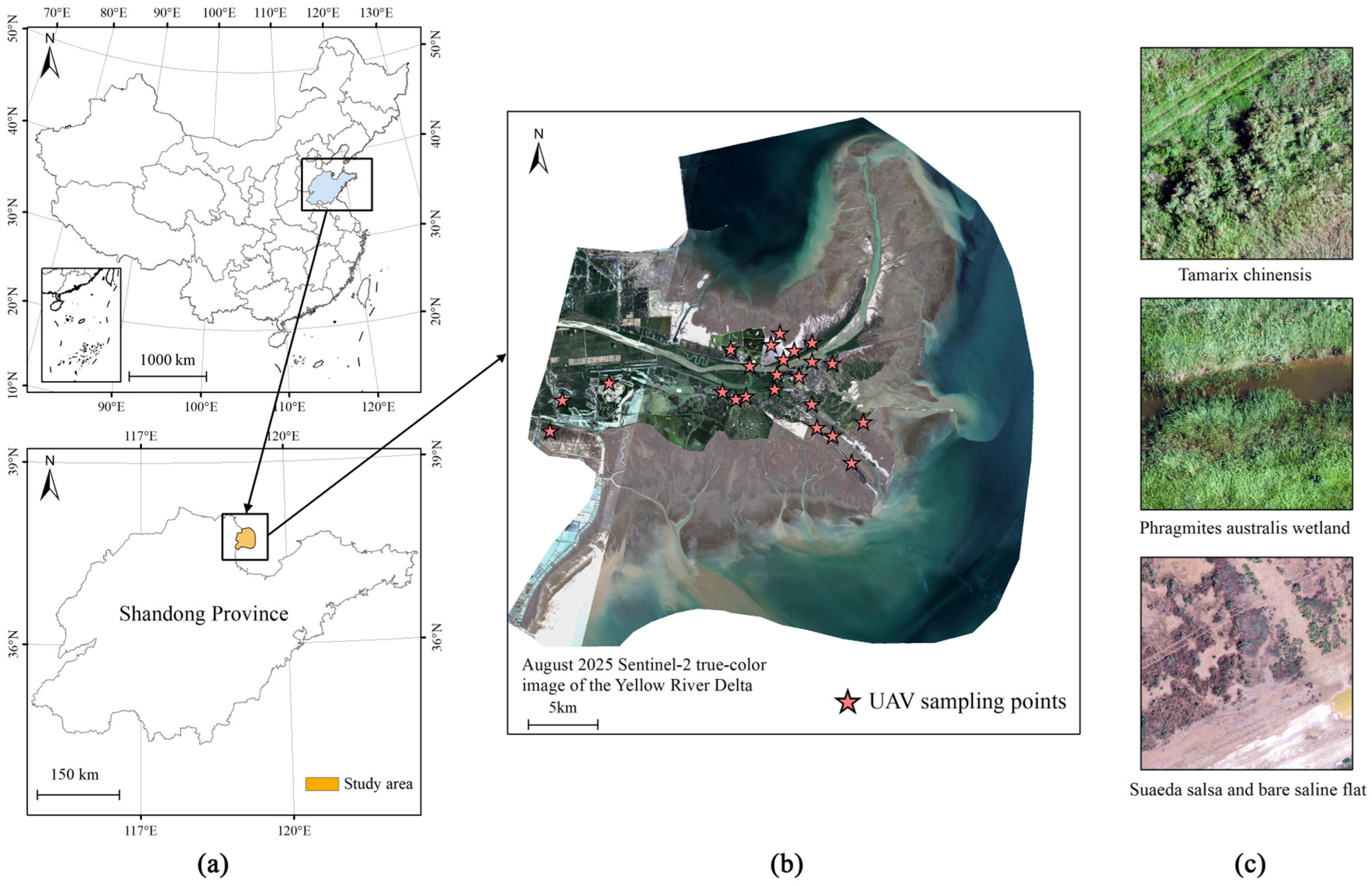
The study area is located in the Yellow River Delta National Nature Reserve in Dongying City, Shandong Province, China, with an approximate geographic extent of 118°33′–119°20′ E and 37°35′–38°12′ N (Figure 1a). The reserve was upgraded to national status in 1992 and was listed as a Wetland of International Importance under the Ramsar Convention in 2013. It is one of the most intact warm-temperate estuarine wetland ecosystems in China [16,29]. The Yellow River carries large amounts of sediment into the sea in this region, forming a flat estuarine delta dominated by coastal saline–alkaline soils and a shallow groundwater table [4]. Under the combined influence of estuarine hydrology, tidal inundation, and soil salinity gradients, vegetation in the reserve shows clear spatial zonation and mosaic patterns. The main vegetation and land-cover types include Phragmites australis, Tamarix chinensis, Suaeda salsa, and tidal flats or saline–alkaline bare land [4,17]. Among them, T. chinensis is commonly distributed in transitional zones between P. australis salt marshes, S. salsa mudflats, and saline–alkaline bare land, forming local patches with varying densities [2,6,16]. The location of the study area and the UAV survey areas are shown in Figure 1a and Figure 1b, respectively, and representative UAV aerial photographs of typical land-cover types are shown in Figure 1c.
Figure 1.
Study area and field survey overview. (a) Geographic location of the Yellow River Delta National Nature Reserve within China; (b) August 2025 Sentinel-2 true-color composite image of the study area with UAV survey areas; (c) Representative UAV aerial photographs of typical land-cover types in the study area. Map lines delineate study areas and do not necessarily depict accepted national boundaries.
2.2. Data and Samples
This study used Sentinel-2 MSI Level-2A surface reflectance products and Sentinel-1 IW GRD dual-polarization (VV/VH) products as the primary remote sensing data sources, supplemented by unmanned aerial vehicle (UAV) orthophotos for sample collection and validation. Sentinel-2 images were acquired through the Google Earth Engine (GEE) platform from available scenes with cloud cover below 5% during July–August 2025, and a median composite image was generated. The acquisition dates and times of the Sentinel-1/2 scenes used in the composites are listed in Table A1, together with the nearest predicted tidal events at Dongying Port. The 20 m resolution bands, including B5, B6, B7, B8A, B11, and B12, were resampled to 10 m using bilinear interpolation. The July–August period was selected because it corresponds to the annual peak growing season of Tamarix chinensis, when the reflectance slope response in the red-edge region is most pronounced [2,26]. Sentinel-1 preprocessing was performed on the GEE platform, including orbit correction, radiometric calibration, and terrain correction based on the SRTM DEM. The backscattering coefficients were expressed in dB [11,30]. Because tidal inundation may influence wetland moisture conditions and SAR/NDWI-related responses, the image acquisition times were compared with the nearest available tidal predictions. This comparison was used as a post hoc contextual check rather than as a tidal correction.
Field sampling was conducted during July–August 2025, concurrent with the remote sensing image acquisition. A three-step validation scheme combining UAV flights, GPS positioning, and visual interpretation of UAV imagery was used [31]. The UAV orthophotos had a ground sampling distance of approximately 2.4–3.0 cm. Sampling followed a stratified random design and covered the main land-cover types, including T. chinensis, Phragmites australis, Suaeda salsa, and bare land or saline–alkaline land. The T. chinensis samples included dense patches, sparse patch edges, and low-cover patches to represent target-species characteristics under different canopy cover conditions. Non-tamarisk samples covered both typical pure patches and background types that are easily confused with T. chinensis, including P. australis salt marshes, S. salsa mudflats, and saline–alkaline bare land. All samples were visually interpreted using UAV orthophotos and GPS records, and class labels were assigned according to the dominant canopy type within the sample pixel and its neighborhood. For samples located at patch edges or in complex backgrounds, labeling prioritized the dominant canopy cover type within the sample pixel to ensure consistency between the training labels and the 10 m Sentinel pixel scale. A total of 771 valid samples were obtained (Table 1) and were divided into training (616 samples) and test (155 samples) sets using an 8:2 stratified random split, with the random seed fixed at 42.
Table 1.
Statistics of training and test samples.
2.3. Feature Construction
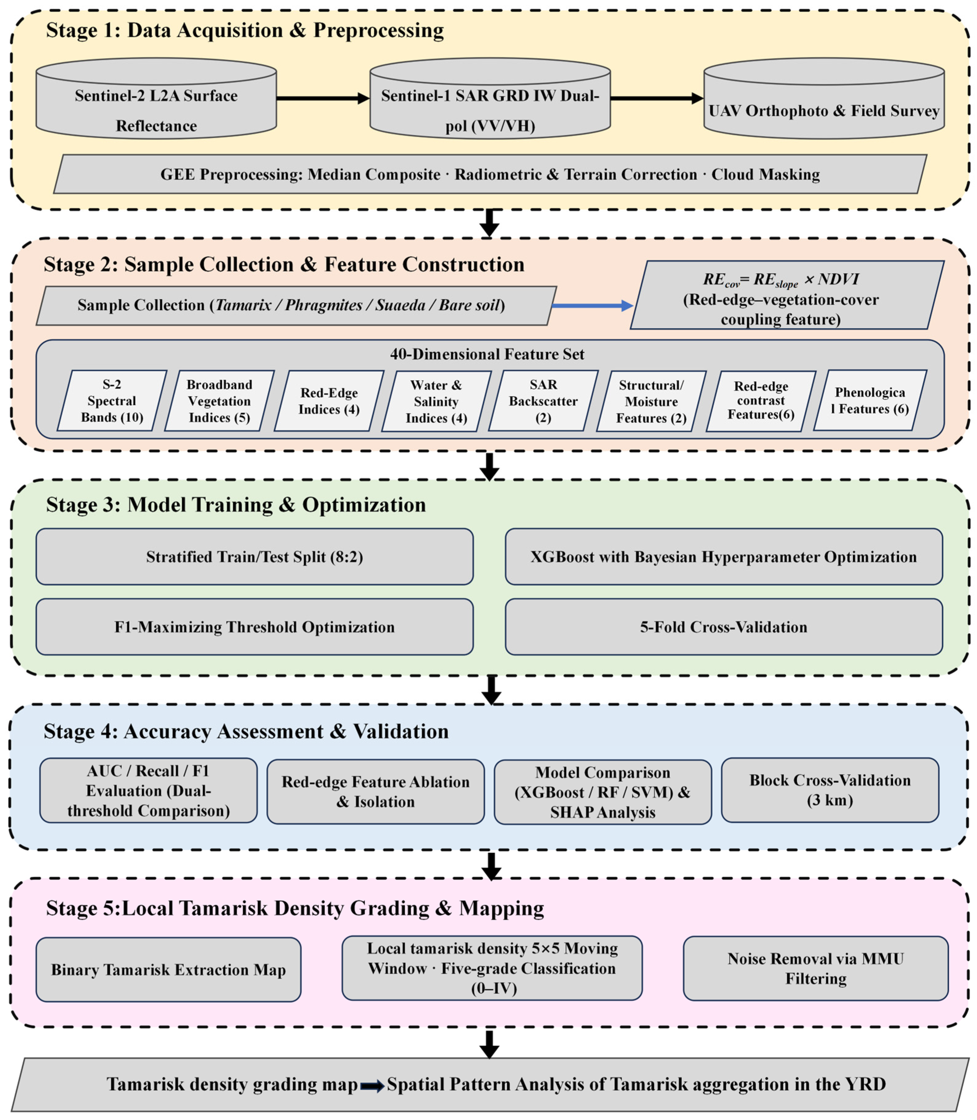
This study constructed a multi-source feature set (Table 2) and used feature ablation and replacement experiments to evaluate the marginal contribution of each candidate feature group to low-omission Tamarix chinensis identification. The overall workflow is shown in Figure 2. The feature set consisted of Sentinel-2 spectral and index features, Sentinel-1 SAR backscatter features, a red-edge–vegetation-cover coupling feature, contrast features between red-edge features and broadband/SWIR indices, and phenological features. Together, these features were used to characterize differences between T. chinensis and co-occurring land-cover types in spectral response, red-edge slope, vegetation cover, moisture and salinity background, canopy structure, and seasonal dynamics.
Table 2.
Multi-source feature set used for classification.
Figure 2.
Workflow of the proposed approach, comprising five stages: (1) data acquisition and GEE-based preprocessing of Sentinel-2, Sentinel-1, and UAV data; (2) sample collection and construction of a 40-dimensional multi-source feature set incorporating the red-edge–vegetation-cover coupling feature (REcov); (3) XGBoost model training and optimization; (4) accuracy assessment and validation, including ablation, model comparison, SHAP analysis, and spatial block cross-validation; and (5) local Tamarix chinensis density grading and mapping.
The Sentinel-2 spectral features included 10 surface reflectance bands: B2, B3, B4, B5, B6, B7, B8, B8A, B11, and B12. Based on these bands, we calculated five broadband vegetation indices, including NDVI, EVI, EVI2, SAVI, and MSAVI, to characterize vegetation greenness and cover status; four red-edge indices, including NDRE, NDRE2, REP, and MTCI, to describe chlorophyll content, red-edge position, and red-edge slope variation; and four water and salinity indices, including NDWI, MNDWI, SI1, and SI2, to provide complementary information on wetland moisture conditions and saline–alkaline bare-land backgrounds. The Sentinel-1 features included the VV and VH backscattering coefficients, which were used to complement the canopy structure and surface moisture differences that optical imagery alone may not fully capture.
To enhance the expression of red-edge information for target-species identification of T. chinensis, we constructed a red-edge–vegetation-cover coupling feature. As described in the Introduction, reNDVI can characterize red-edge slope differences within the Sentinel-2 B5–B6 interval (hereafter denoted as REslope) and is sensitive to differences in red-edge responses between T. chinensis and co-occurring herbaceous vegetation. However, at the 10 m pixel scale, low-density T. chinensis patches are often mixed with background components such as saline–alkaline bare land, Suaeda salsa, or standing water. These non-target components can alter the overall pixel reflectance, causing the red-edge slope to be influenced by both species differences and vegetation cover. A weaker red-edge response may therefore result either from interspecific spectral differences or from background mixing caused by insufficient effective vegetation cover. NDVI is a commonly used proxy for green vegetation activity and cover status, and can provide an effective vegetation-signal constraint for red-edge responses. Therefore, we coupled the red-edge slope term with NDVI through multiplication to obtain the red-edge–vegetation-cover coupling feature, REcov:
In Equations (1)–(7), ε is a small constant set to 10−8 to avoid division by zero. This coupling feature is designed to preserve red-edge slope differences in pixels with clear vegetation signals while suppressing the interference of unstable red-edge responses from low-cover or saline–alkaline background pixels in the classification model. To further examine the behavior of this multiplicative construction under mixed-pixel conditions, we conducted a sample-derived random-pair mixture sensitivity analysis between Tamarix chinensis and Suaeda salsa spectra. For each mixture fraction, Sentinel-2 reflectance bands were linearly mixed first, and NDVI, REslope, and REcov were then recalculated from the mixed bands.
In addition to the red-edge–vegetation-cover coupling feature, we further calculated the red-edge-to-narrow-NIR structural feature REnir and the near-infrared-to-shortwave-infrared moisture feature, NDMI:
where REnir characterizes reflectance variation from the later red-edge region to the narrow near-infrared region, and NDMI characterizes differences in vegetation moisture and wet–dry background conditions between the near-infrared and shortwave-infrared regions. Both features were included in the model as independent candidate features, and no multiplicative term was constructed between them.
REnir = (B8A − B7)/(B8A + B7 + ε)
NDMI = (B8 − B11)/(B8 + B11 + ε)
To further enhance the spectral contrast between Tamarix chinensis and co-occurring vegetation, we constructed contrast features based on REcov and conventional vegetation indices, including REcov-EVI, REcov-NDRE, and NDVI-REcov. We also constructed a red-edge-SWIR composite response term, RESWIR, based on the later red-edge, shortwave-infrared, and red bands:
Based on this term, RESWIR-NDRE, RESWIR-EVI, and NDVI-RESWIR were calculated. These six contrast features were used to strengthen the relative differences among red-edge, greenness, and shortwave-infrared responses, and were included as candidate features in the classification model. To test whether the red-edge–vegetation-cover coupling feature provided additional information relative to general red-edge indices, the replacement experiments used an equal number of IRECI-derived features, IRECI = (B7 − B4)/(B5/B6), and CLre-derived features, CLre = (B7/B5 − 1), constructed using the same logic to replace the above REcov-derived features as controls (see Section 3.2).
Phenological features were used to characterize differences in seasonal dynamics between T. chinensis and herbaceous salt-marsh vegetation. Spring, summer, and autumn features were derived from Sentinel-2 composites for March–May, July–August, and September–November of 2025, respectively, using the same cloud-cover filtering and compositing procedure described in Section 2.2. Seasonal NDVI and EVI refer to index values calculated from these seasonal composites, rather than curve-fitted phenological transition metrics. Therefore, SOS, EOS, and POP were not derived in this study. Specifically, the phenological feature set included spring NDVI, spring EVI, autumn NDVI, the summer–spring NDVI difference, the summer–autumn NDVI difference, and the phenological asymmetry ratio (Equation (7)). The phenological asymmetry ratio was defined as:
where spr, sum, and aut denote spring, summer, and autumn, respectively; ΔNDVIspr–sum represents the NDVI change from spring to summer, ΔNDVIsum–aut represents the NDVI change from summer to autumn, and ε is a small constant set to 1 × 10⁻⁸ to avoid division by zero. This ratio was used to describe differences between vegetation change from spring green-up to the summer peak and vegetation change from the summer peak to autumn senescence. All features and their functional descriptions are listed in Table 2.
2.4. Model Training and Evaluation
In this study, the XGBoost algorithm [32] was used to construct a binary classification model for Tamarix chinensis, and key hyperparameters were determined through Bayesian optimization (Table 3). Considering the imbalance between T. chinensis (positive class) and non-tamarisk samples, scale_pos_weight was set to 1.5 as a moderate class-imbalance adjustment. This setting was used to reduce the influence of class imbalance during model training and was not intended to represent a formal cost matrix. Model stability was confirmed using five-fold cross-validation (CV F1 = 0.8576). The classification threshold was selected from the five-fold cross-validation threshold curve on the training set. The threshold of 0.43 was retained as the operating threshold because it maximized F1 while maintaining high Tamarix recall. The test set was used only for final performance reporting and was not involved in threshold or hyperparameter selection. To evaluate the influence of algorithm choice, Random Forest and SVM models were trained as baselines under the same conditions, including the same feature set, scale_pos_weight = 1.5, threshold = 0.43, and random_state = 42.
Table 3.
Optimized hyperparameters of the XGBoost classifier.
Model performance was evaluated using OA, Precision, Recall, F1, AUC, and SHAP feature importance [21,33]. To assess the marginal contribution of the red-edge-oriented contrast features, feature ablation and replacement experiments were designed. With all other features, hyperparameters, and random seeds fixed, we separately removed the REcov-derived features, the RESWIR-derived features, and all red-edge contrast features. We also used an equal number of IRECI- and CLre-derived features constructed using the same logic as replacement controls. All schemes were evaluated on the same test set. To assess the influence of spatial autocorrelation, spatial block cross-validation was additionally performed using 3 km blocks and 15 folds, with the mean and standard deviation of AUC used as conservative estimates of spatial generalization ability [34].
2.5. Local Density Grading of Tamarix chinensis
Based on the classification result after vegetation masking, in which water bodies and bare land were excluded and only valid vegetation pixels were retained, we calculated the proportion of Tamarix chinensis pixels within a 5 × 5 neighborhood window centered on each pixel. This window corresponds to approximately 50 m × 50 m in the field and is consistent with commonly used scales for spatial analysis of shrub patches [35,36]. The proportion of Tamarix chinensis pixels relative to the total number of vegetation pixels within the window was defined as the local tamarisk density of the center pixel:
where Ntamarisk is the number of Tamarix chinensis pixels within the window, and Nvegetation is the total number of vegetation pixels within the window, including Tamarix chinensis. When Nvegetation = 0, the pixel was assigned NoData. The resulting proportion raster retained a spatial resolution of 10 m, and all area statistics were calculated based on 10 m pixels, with each pixel representing 100 m2. This proportion represents the local occurrence frequency of Tamarix chinensis at the pixel scale rather than field-measured ground cover; therefore, the two are not directly equivalent in numerical terms.
Based on the continuous distribution of local density, we divided the raster into five operational grades to support patrol planning and stratified management in the protected area (Table 4). Absolute absence (0%) was separated from trace occurrence (>0%–10%) to distinguish areas without detected tamarisk from early or sparse occurrence zones. The thresholds of 10%, 30%, and 60% were then used to distinguish trace, sparse, moderate-density, and high-density aggregation areas for stratified patrol planning.
Table 4.
Local tamarisk density grades.
3. Results
3.1. Spectral Characteristics of Tamarix chinensis and Typical Vegetation
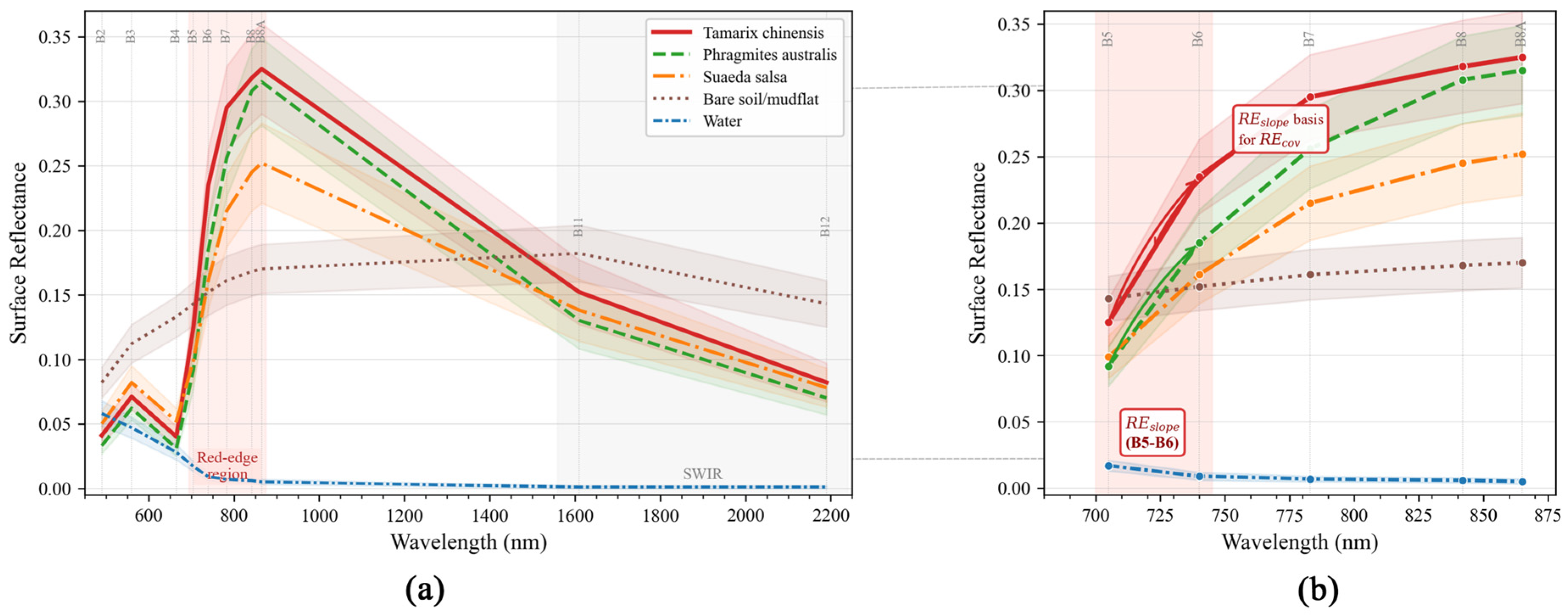
Figure 3 shows the mean Sentinel-2 reflectance curves of five typical land-cover types in the study area: Tamarix chinensis, Phragmites australis, Suaeda salsa, bare saline–alkaline land, and water. In the broad visible-to-near-infrared range from B2 to B8, the reflectance curves of Tamarix chinensis and Phragmites australis showed similar overall trends and a high degree of overlap. This is consistent with the fact that both species have relatively high green biomass during the summer peak growing season and are difficult to distinguish using broadband spectral information alone. In the red-edge region, however, the two species showed observable differentiation. Tamarix chinensis exhibited a larger increase in reflectance from B5 (705 nm) to B6 (740 nm) than Phragmites australis, indicating a steeper red-edge slope. Suaeda salsa had lower reflectance in the near-infrared region from B7 to B8A than Tamarix chinensis and Phragmites australis, whereas bare saline–alkaline land showed clearly high values in the shortwave-infrared bands B11 and B12. These patterns indicate that the spectral responses of Suaeda salsa and bare saline–alkaline land were more clearly differentiated from those of the vegetation classes.
Figure 3.
Sentinel-2 surface reflectance spectral profiles of five typical land-cover types in the study area. (a) Full spectral range (560–2200 nm). (b) Enlarged view of the red-edge region (680–865 nm); the shaded area marks the B5–B6 interval, where Tamarix chinensis exhibits a steeper red-edge slope than co-occurring vegetation. Shaded bands represent ± one standard deviation. Sentinel-2 band positions are indicated along the top axis.
The red-edge slope difference in the B5–B6 interval provided the spectral basis for constructing the red-edge–vegetation-cover coupling feature, REcov, in this study. The actual marginal contribution of this feature to classification performance was further quantitatively evaluated through the ablation and replacement experiments described in Section 3.2.
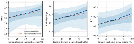
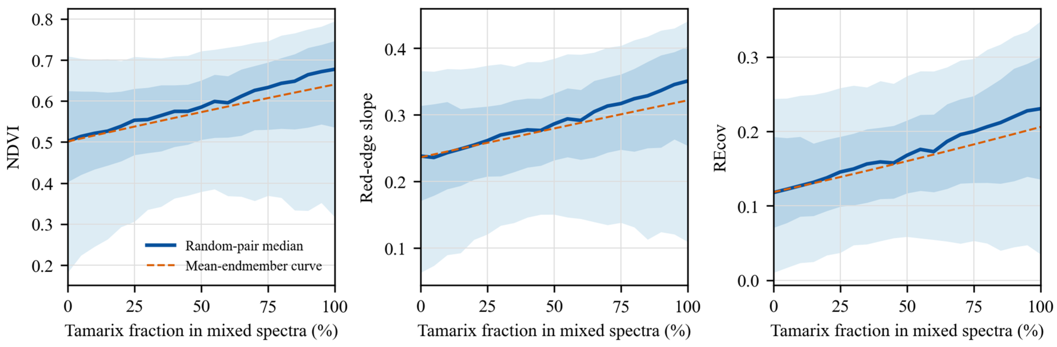
To further examine the response of REcov under mixed-pixel conditions, we performed a random-pair mixture analysis using sample spectra of Tamarix chinensis and Suaeda salsa (Figure 4). Across the simulated mixture gradient, the median values of NDVI, REslope, and REcov increased with the Tamarix fraction, while the 5%–95% intervals retained substantial sample-level variability. This result indicates that REcov responds consistently to increasing Tamarix spectral contribution, but should be interpreted as an empirical mixed-pixel sensitivity check rather than as a universal physiological index.
Figure 4.
Sample-derived random-pair mixture sensitivity of NDVI, red-edge slope, and REcov between Tamarix chinensis and Suaeda salsa. For each mixture fraction, Tamarix and Suaeda sample spectra were randomly paired, Sentinel-2 reflectance bands were linearly mixed, and the indices were recalculated from the mixed bands. The solid line represents the median response, shaded bands represent the 25%–75% and 5%–95% intervals, and the dashed line represents the mean–endmember curve.
3.2. Classification Accuracy Assessment
3.2.1. Main Model Accuracy and Threshold Selection
For the main XGBoost model, which used the full REcov-based feature set, scale_pos_weight = 1.5, and Bayesian-optimized hyperparameters, the classification threshold was selected from the five-fold cross-validation threshold curve on the training set, and 0.43 was retained as the fixed operating threshold. The test set was used only for final performance reporting and was not involved in threshold or hyperparameter selection. On the independent test set (n = 155; 106 Tamarix chinensis samples and 49 non-tamarisk samples), the model achieved an AUC of 0.8042, and the five-fold cross-validation F1 was 0.8576. At the selected threshold of 0.43, the Precision, Recall, F1, and OA for the Tamarix chinensis class were 0.8250, 0.9340, 0.8765, and 0.8194, respectively. The confusion matrix was TP/FN/FP/TN = 99/7/21/28.
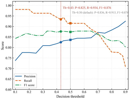
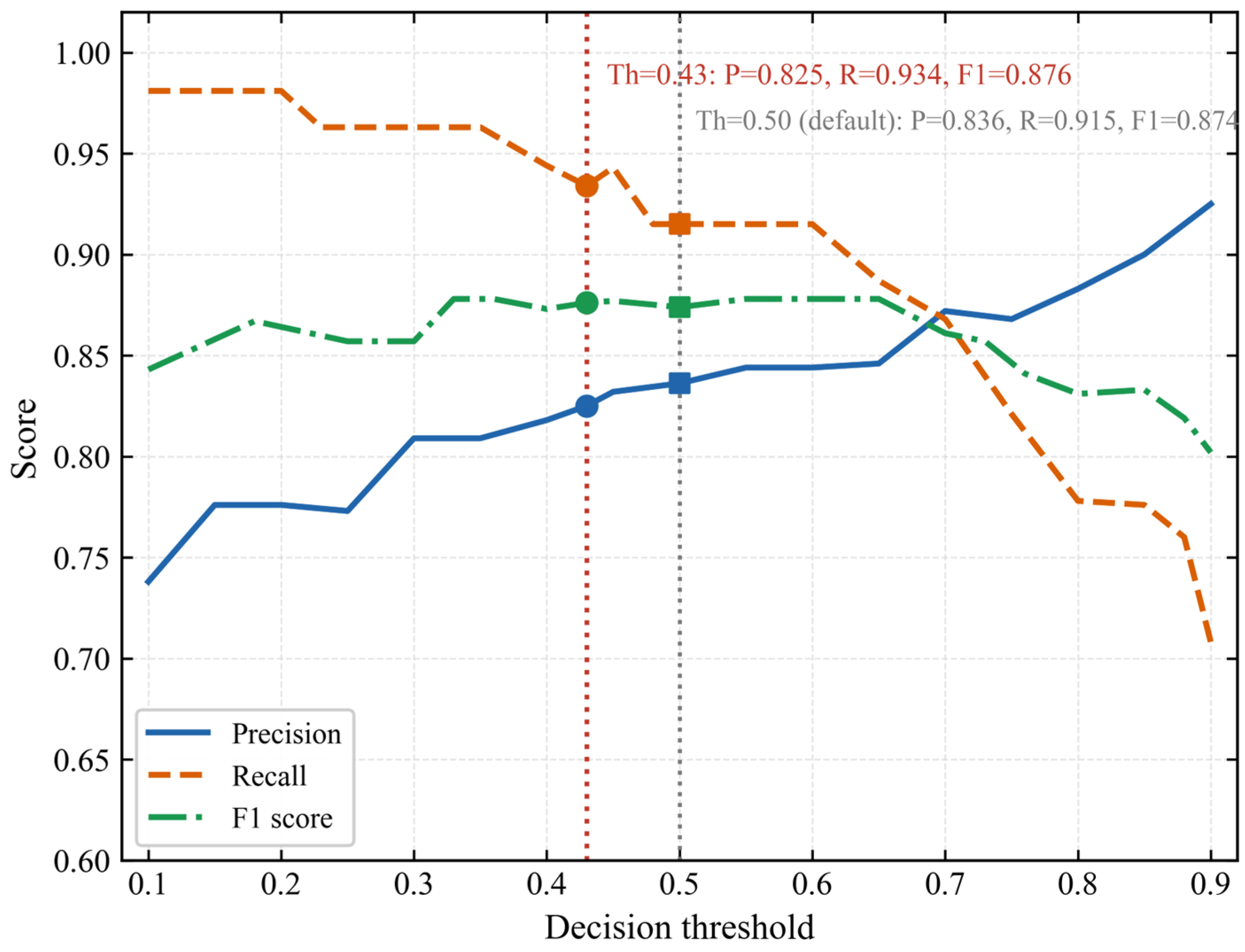
To evaluate the sensitivity of test-set metrics to the decision threshold, Table 5 and Figure 5 compare the selected threshold of 0.43 with the default threshold of 0.50. It should be noted that the threshold had already been determined within cross-validation; this comparison was used only to illustrate the robustness of test-set performance to threshold choice, rather than to reselect the threshold on the test set. When the threshold increased from 0.43 to 0.50, Recall decreased from 0.9340 to 0.9151, and FN increased from 7 to 9. Precision increased from 0.8250 to 0.8362, F1 decreased from 0.8765 to 0.8717, and OA remained stable at 0.8194 under both thresholds. AUC was identical under the two thresholds (0.8042), because AUC is independent of the classification threshold. This threshold was selected before final test-set reporting and was used as a fixed operating threshold for subsequent model comparison and ablation experiments.
Table 5.
Classification accuracy comparison between threshold = 0.43 and threshold = 0.50.
Figure 5.
Classification performance metrics (Precision, Recall, and F1 score) as a function of decision threshold for the XGBoost model on the test set. The red dotted vertical line indicates the selected threshold of 0.43 (Recall = 0.9340, F1 = 0.8765, Precision = 0.8250); the grey dotted vertical line indicates the default threshold of 0.50 (F1 = 0.8717, Recall = 0.9151). Filled markers denote the metric values at each annotated threshold.
3.2.2. Ablation and Spatial Block Validation
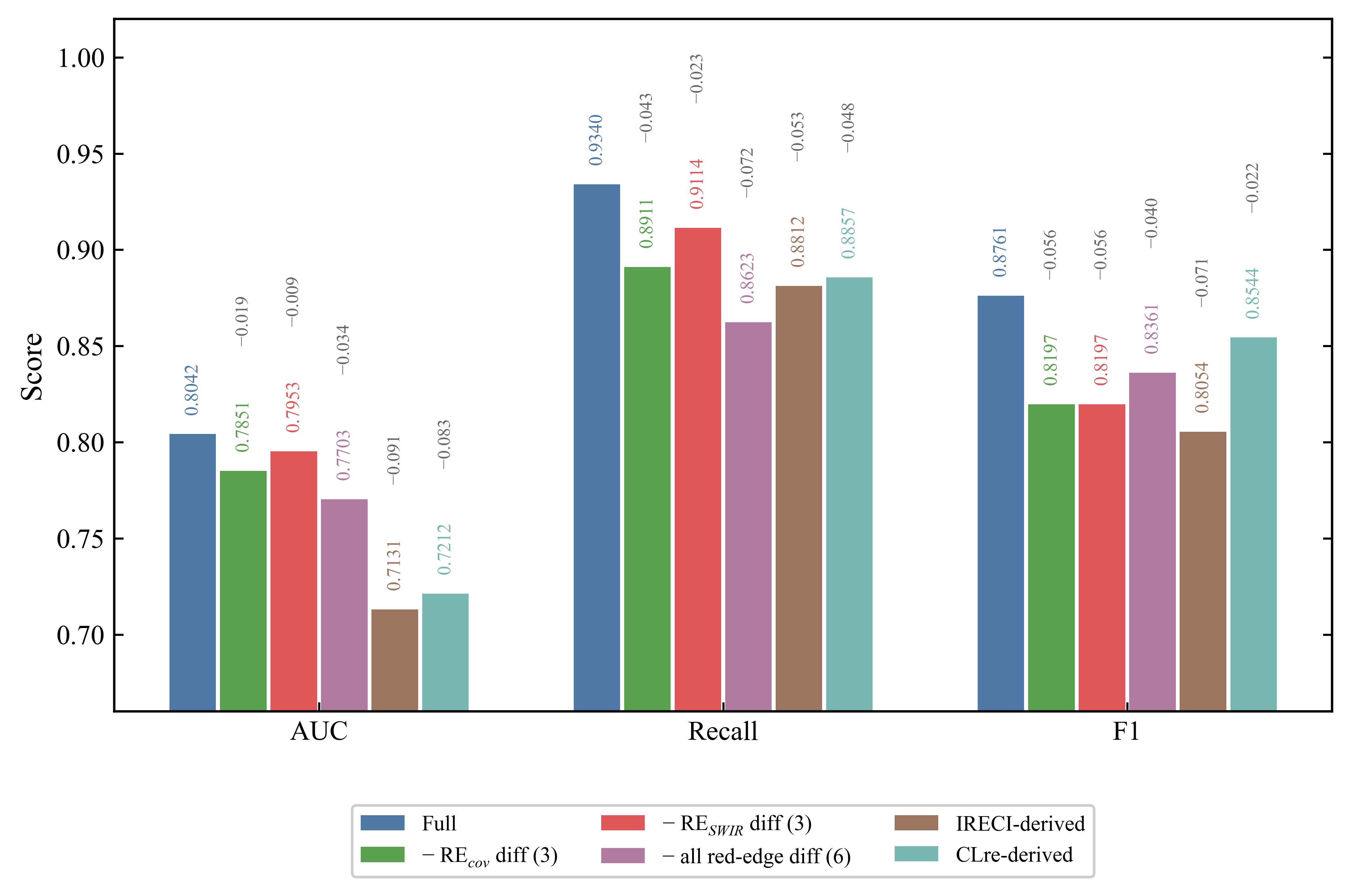
To evaluate the marginal contribution of the red-edge-oriented contrast features within the multi-source feature set, we removed each group of red-edge contrast features and retrained the model while keeping all other features, hyperparameters, and random seeds fixed (Table 6). When the three REcov-derived contrast features were removed, AUC decreased from 0.8042 to 0.7851 (ΔAUC = −0.019), and Recall decreased from 0.9340 to 0.8911. When the three RESWIR-derived contrast features were removed, AUC decreased to 0.7953 (ΔAUC = −0.009), and Recall decreased to 0.9114. When all six red-edge contrast features were removed, AUC decreased to 0.7703 (ΔAUC = −0.034), and Recall decreased to 0.8623. These results indicate that the red-edge-oriented contrast features contributed to both positive–negative class separability, as measured by AUC, and tamarisk recall, with both metrics decreasing after feature removal. Between the two feature groups, the individual contribution of REcov (ΔAUC = −0.019) was greater than that of RESWIR (ΔAUC = −0.009), suggesting that the overall gain came from the combined effect of these features, with the red-edge–vegetation-cover coupling branch contributing more strongly.
Table 6.
Ablation of red-edge-oriented difference features on the test set.
To test whether the red-edge-oriented contrast features provided additional information relative to general red-edge indices, we replaced them with an equal number of IRECI-derived and CLre-derived features constructed using the same logic, and repeated the experiments under the same training conditions. The AUC values of the IRECI-derived and CLre-derived schemes were 0.7131 and 0.7212, respectively, both lower than that of the proposed scheme. CLre performed slightly better than IRECI, consistent with the fact that its B7/B5 ratio implicitly contains part of the red-edge slope information. However, both replacement schemes performed worse than the scheme that explicitly modeled the red-edge slope, indicating that the targeted construction based on red-edge slope differences between tamarisk and Phragmites australis provided additional separability information compared with general chlorophyll-related red-edge indices. The comparative results of the ablation and replacement schemes are summarized in Figure 6.
To compare the effects of different constructions of the red-edge-cover contrast features, we tested three alternative configurations based on the full scheme (REcov = REslope × NDVI): removing this group of contrast features, replacing it with the raw red-edge slope REslope, and replacing it with an additive combination of REslope and NDVI rather than a multiplicative coupling. All other conditions were kept unchanged (Table 7). The AUC of the raw red-edge slope scheme (0.8033) was close to that of the multiplicative scheme (0.8042), whereas the additive scheme was slightly lower (0.7903). However, at the fixed threshold of 0.43, the Recall of the multiplicative scheme (0.9340) was higher than that of the raw slope scheme (0.8044) and the additive scheme (0.8111), with a correspondingly higher OA.
Table 7.
Isolation ablation of the red-edge–vegetation coupling construction.
To examine the robustness of these results under spatial blocking, we performed spatial block cross-validation at a 3 km block scale. The AUC of the full scheme was 0.770, and decreased to 0.687 after all six red-edge contrast features were removed (ΔAUC = −0.083). Among the two feature groups, removing the REcov-derived features caused a larger AUC decrease (−0.022) than removing the RESWIR-derived features (−0.005). The AUC from spatial block cross-validation was generally lower than that from random cross-validation, but the decreasing trend after removing the red-edge contrast features remained consistent. This indicates that the contribution of this feature group to separability remained evident under spatial block validation.
Figure 6.
Ablation results across feature configurations. Bars show AUC, Recall, and F1; Δ values are relative to the full feature set.
3.2.3. Model Comparison
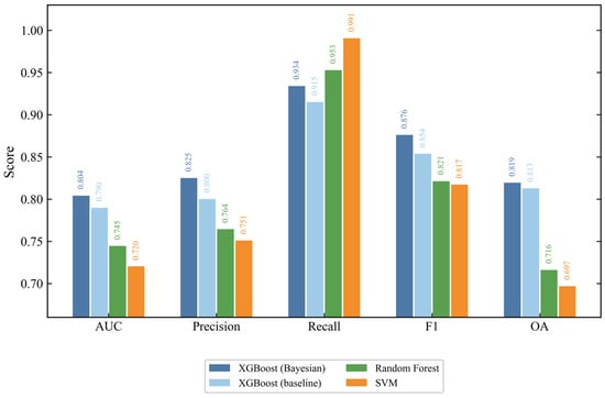
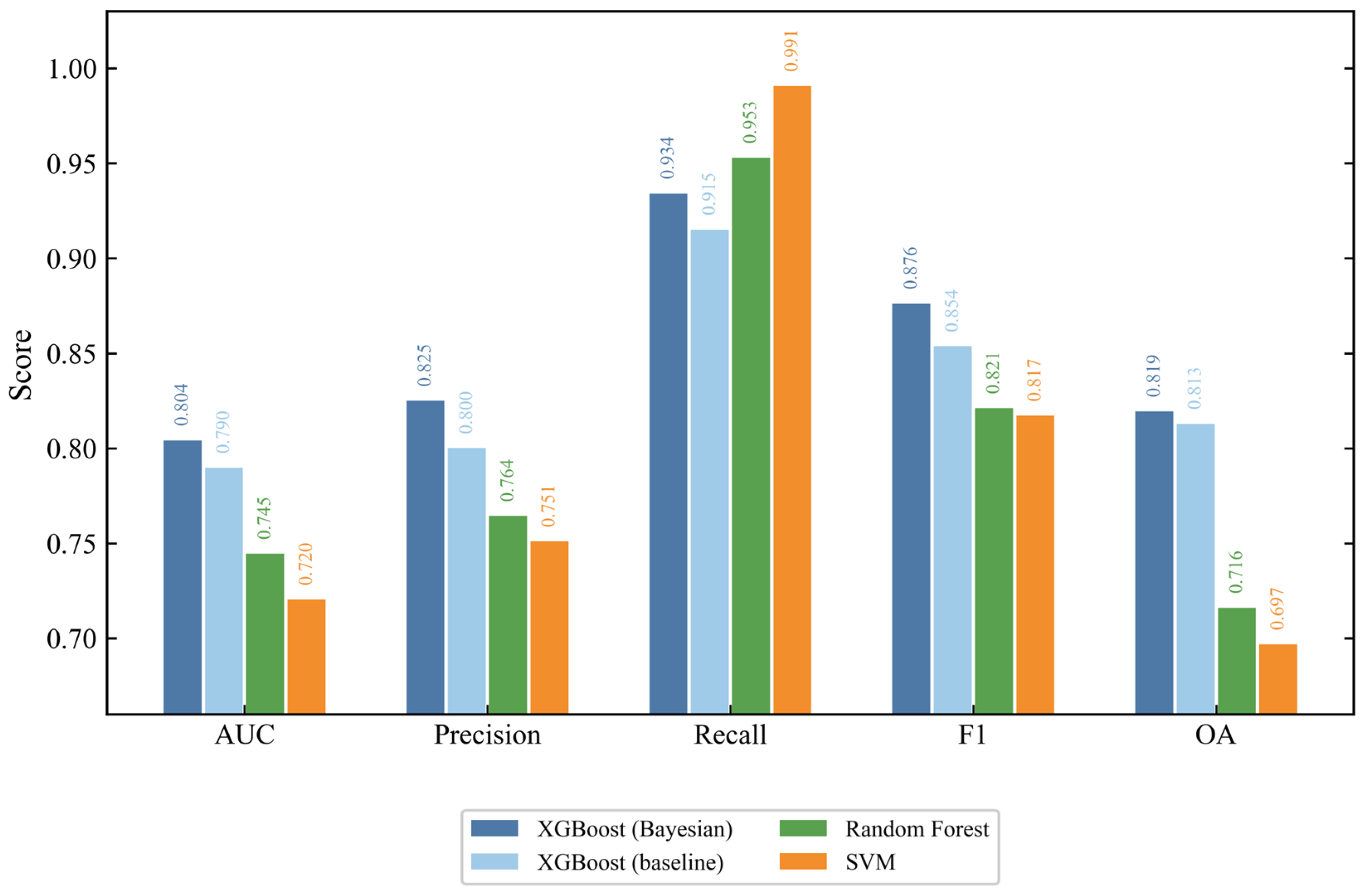
Figure 7 presents the accuracy metrics of four models under unified conditions: 40-dimensional feature set, scale_pos_weight = 1.5, random_state = 42, and the same threshold of 0.43 for all models to facilitate comparison. Using the threshold-independent AUC as the main comparison criterion, the Bayesian-optimized XGBoost model ranked first with an AUC of 0.8042, followed by the XGBoost baseline with default hyperparameters (0.7897), Random Forest (0.7445), and SVM (0.7203). These results indicate that the gradient boosting framework outperformed Random Forest and SVM in this task, and that hyperparameter optimization provided a further improvement.
Figure 7.
Performance comparison of four classifiers under identical conditions (40-dimensional feature set, threshold = 0.43, scale_pos_weight = 1.5, random_state = 42). XGBoost (baseline) uses default hyperparameters without Bayesian optimization. Metrics are reported for the tamarisk class.
For threshold-dependent metrics, SVM achieved the highest Recall (0.9906), but its OA (0.6968) and F1 (0.8171) were markedly lower than those of XGBoost, indicating that its high recall came at the cost of many non-tamarisk false positives. Random Forest also showed a high Recall (0.9528), but its F1 (0.8211) and OA (0.7161) were likewise substantially lower than those of XGBoost. The main XGBoost model achieved the best F1 (0.8765) and OA (0.8194), providing a better balance between recall and precision, while maintaining a high Recall (0.9340). Considering both AUC and the threshold-dependent metrics, the Bayesian-optimized XGBoost model was selected as the optimal model for this task [21,24].
3.2.4. SHAP Feature Importance
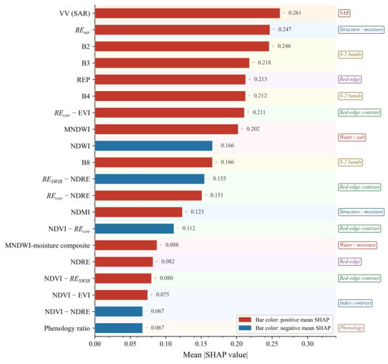
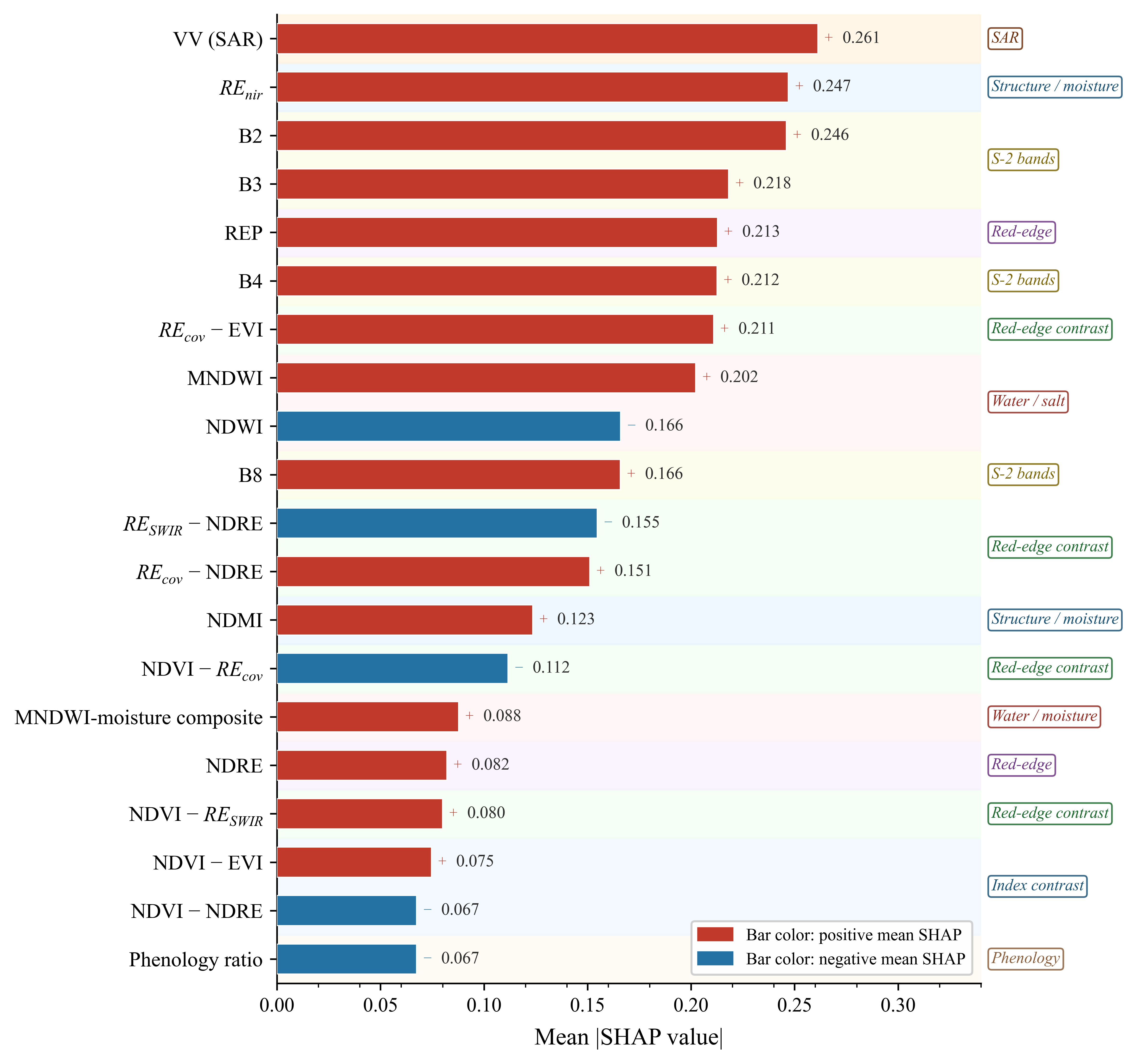
Figure 8 shows the top 20 feature-importance ranking of the main XGBoost model based on the SHAP method, measured by the mean absolute SHAP value on the test set. The VV backscattering coefficient ranked first (mean |SHAP| = 0.261), followed by REnir (0.247) and B2 (0.246). These were followed by B3 (0.218), REP (0.213), and B4 (0.212), indicating that SAR backscatter, the later red-edge-to-near-infrared structural feature, and the visible and red-edge bands jointly constituted the main information sources for distinguishing Tamarix chinensis from co-occurring land-cover types.
Figure 8.
SHAP-based feature-importance ranking of the top 20 features in the XGBoost classifier. Bar length is the mean absolute SHAP value across the test set; red and blue indicate positive and negative mean SHAP directions, respectively. Feature groups are annotated on the right axis: SAR, structure/moisture, Sentinel-2 spectral bands, red-edge bands, water/salt indices, red-edge contrast (REcov/RESWIR difference features), index contrast, and phenology.
The red-edge-oriented contrast features also entered the top 20 as a group. REcov-EVI (0.211) ranked 7th, RESWIR-NDRE (0.155) ranked 11th, REcov-NDRE (0.151) ranked 12th, and NDVI-REcov (0.112) ranked 14th. At the group level, the mean absolute SHAP value of the REcov-derived features (0.211, 0.151, 0.112) was higher than that of the RESWIR-derived features, and REcov-EVI was the highest-ranked red-edge contrast feature overall. This is consistent with the ablation results, in which removing the REcov-derived features caused a more pronounced decrease in AUC and Recall. Together, these two feature groups provided separability information from the red-edge region and supported tamarisk recall. In addition, the independent structural/moisture feature NDMI (0.123) ranked 13th and was also among the top 20 features.
3.3. Spatial Distribution of Extracted Tamarisk
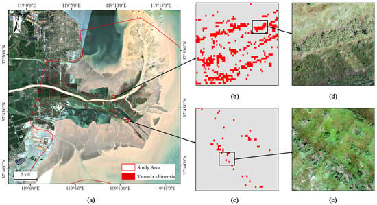
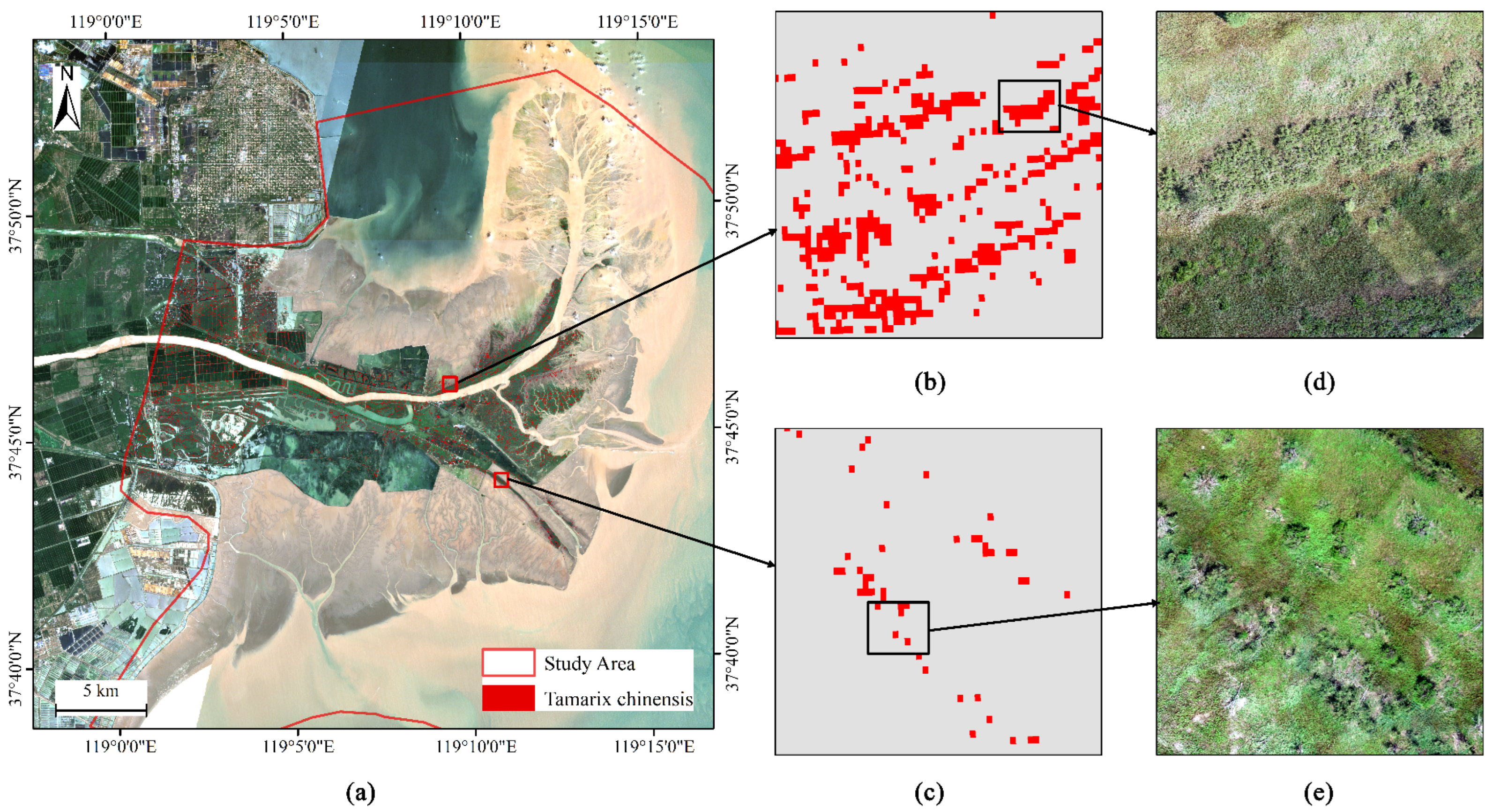
The full-extent extraction result based on the XGBoost model showed that the total extracted area of T. chinensis in the study area was approximately 12.88 km2, corresponding to 128,833 pixels. Figure 9a shows the spatial distribution of T. chinensis, with the red overlay superimposed on the Sentinel-2 true-color composite basemap. Figure 9b presents an enlarged view of a typical dense T. chinensis patch, where the red overlay is spatially continuous and the patch boundary is relatively clear; the corresponding UAV orthophoto in Figure 9d shows continuous T. chinensis canopy cover, indicating good spatial consistency with the classification result at the 10 m pixel scale.
Figure 9.
Spatial distribution of extracted Tamarix chinensis in the Yellow River Delta National Nature Reserve. (a) Full-extent extraction map overlaid on an August 2025 Sentinel-2 true-color composite. (b) Enlarged view of the dense T. chinensis patch indicated by the upper red rectangle in panel (a). (c) Enlarged view of the sparse, low-density area indicated by the lower red rectangle in panel (a). (d) UAV orthophoto corresponding to the black rectangle in panel (b). (e) UAV orthophoto corresponding to the black rectangle in panel (c).
Figure 9c shows an enlarged view of a sparse, low-density area, where the red patches appear as discrete fragments within a gray-toned mixed background. The corresponding UAV orthophoto in Figure 9e shows that T. chinensis occurs as discrete individuals or small clusters within a P. australis matrix, consistent with the scattered patches identified in the classification result.
3.4. Local Tamarisk Density
After MMU filtering with a threshold of 4 pixels and 8-neighbor connectivity, the pixel count and corresponding area of each density grade are shown in Table 8. Grade 0 (0%) contained 407,485 pixels, corresponding to approximately 40.75 km2. Grade I (>0%–10%) contained 120,748 pixels, corresponding to approximately 12.07 km2. Grade II (10%–30%) contained 19,974 pixels, corresponding to approximately 2.00 km2. Grade III (30%–60%) contained 3634 pixels, corresponding to approximately 0.36 km2. Grade IV (>60%) contained 4036 pixels, corresponding to approximately 0.40 km2. In total, there were 555,877 valid vegetation pixels, covering approximately 55.59 km2. The number of Grade IV pixels (4036) was slightly higher than that of Grade III pixels (3634).
Table 8.
Pixel count and area statistics of local tamarisk density grades after MMU filtering.
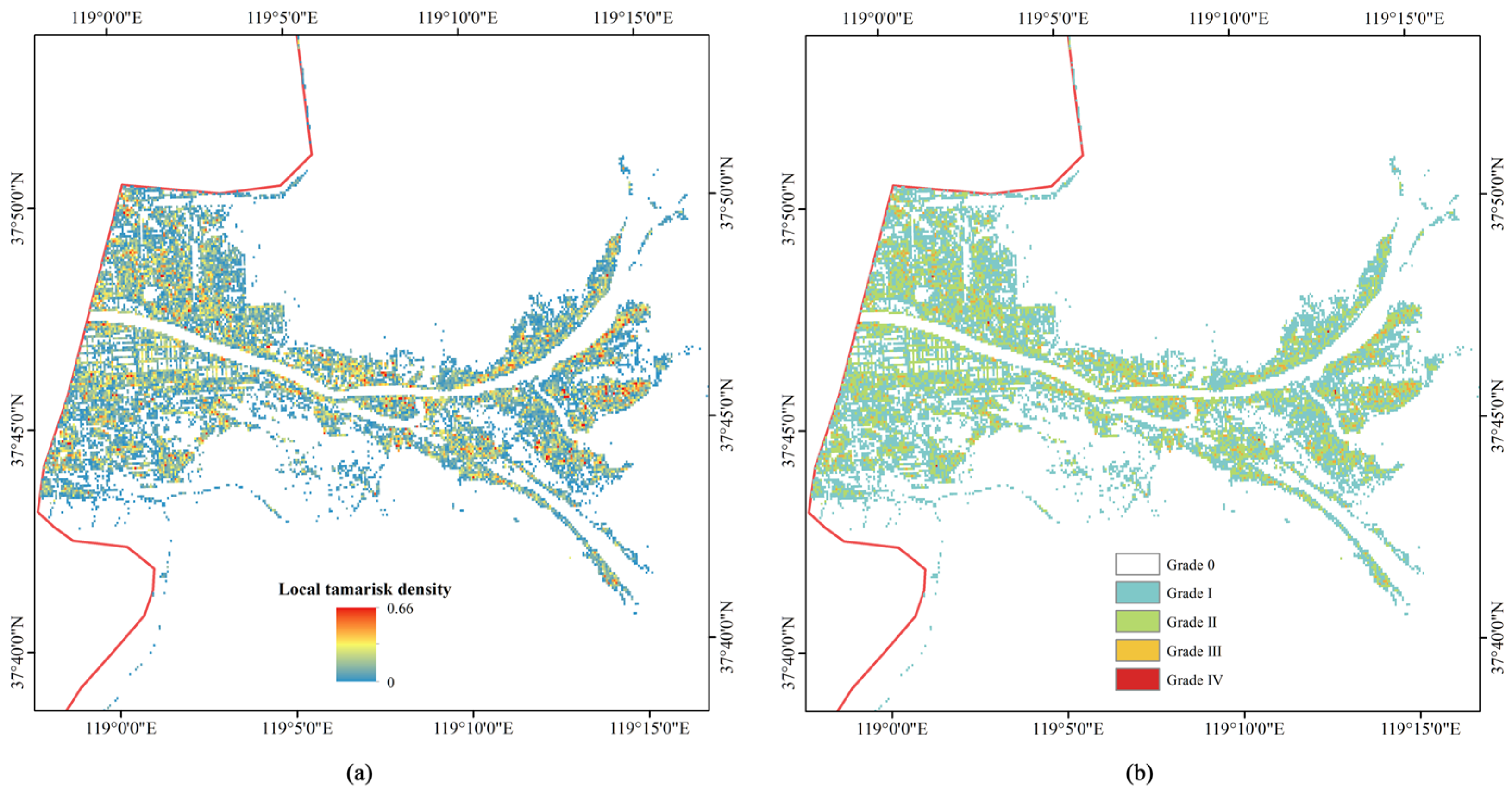
The thematic map of local density grades is shown in Figure 10. High-density areas (Grades III-IV) were spatially clustered, while Grade II areas were distributed around them. Grade 0 (absence) accounted for 73.3% of valid vegetation pixels, whereas Grade I (trace occurrence, >0%–10%) accounted for 21.7%. Together, these two low-density classes represented 95.0% of valid vegetation pixels, indicating a distribution pattern in which the study area was dominated by non-tamarisk vegetation, with Tamarix chinensis occurring as locally aggregated patches.
Figure 10.
Local tamarisk density grading map of Tamarix chinensis in the Yellow River Delta National Nature Reserve. (a) Continuous local tamarisk density computed within a 5 × 5 pixel (50 m × 50 m) moving window, with the output raster retaining the original 10 m resolution and values ranging from 0 to 0.66. (b) Discrete five-grade density classification: Grade 0 (0%, absence), Grade I (>0%–10%, trace), Grade II (10%–30%, sparse), Grade III (30%–60%, moderate), and Grade IV (>60%, dense). Red polygons delineate the study area boundary. Results are shown after MMU filtering with a minimum mapping unit of four pixels and 8-connectivity.
4. Discussion
4.1. Contribution of the Red-Edge–Vegetation-Cover Coupling Feature to Tamarix chinensis Identification
The ablation experiments provided direct evidence for the contribution of the red-edge–vegetation-cover coupling feature. After all six red-edge-oriented contrast features were removed, AUC decreased from 0.8042 to 0.7703 (ΔAUC = −0.034), and Recall decreased from 0.9340 to 0.8623. The simultaneous decrease in both metrics indicates that this feature group improved both positive–negative class separability and tamarisk recall. Between the two feature branches, removing the REcov-derived features alone caused a larger AUC decrease (−0.019) than removing the RESWIR-derived features (−0.009), and this difference remained evident under 3 km spatial block cross-validation (REcov: −0.022; RESWIR: −0.005). These results suggest that the red-edge–vegetation-cover coupling branch made a stronger contribution within this feature group, and that its effect was not dependent on a specific sample split.
The index replacement experiments further revealed the source of the effective information. When the red-edge-oriented contrast features were replaced by general red-edge indices constructed using the same logic, the AUC values of the IRECI-derived and CLre-derived schemes decreased to 0.7131 and 0.7212, respectively, both lower than that of the proposed scheme. CLre performed slightly better than IRECI, consistent with the fact that its B7/B5 ratio implicitly contains part of the red-edge slope information. However, both schemes performed worse than the scheme that explicitly modeled the red-edge slope. This indicates that the information effective for tamarisk identification originated from red-edge slope features rather than the absolute level of chlorophyll content. This result is consistent with the existing understanding that, as a woody shrub, Tamarix chinensis differs from herbaceous Phragmites australis in canopy and leaf structure. Such structural differences can be expressed as detectable red-edge slope differences in the B5–B6 interval [2,14,26], whereas general indices that mainly reflect chlorophyll level may not capture this distinction.
Although the red-edge–vegetation-cover coupling feature did not rank first in the SHAP ranking, with REcov-EVI ranking 7th and having a mean absolute SHAP value of 0.211, it had a clear effect on model performance in the ablation experiments. This contrast reflects the difference between single-feature importance and feature-group contribution. SHAP measures the average marginal attribution of each feature within the existing feature set, whereas ablation measures the net loss in model capability after an entire feature group is removed. The top-ranked features, including VV (0.261), REnir (0.247), and B2 (0.2246), provided strong overall discriminatory signals related to SAR backscatter, canopy structure, and visible reflectance. However, these signals are highly overlapped in transitional zones between tamarisk and co-occurring herbaceous vegetation. The contribution of the red-edge–vegetation-cover coupling feature was therefore not the largest overall variance signal, but rather an incremental separability signal that acted on the most easily confused samples. Its effect became fully apparent only when the whole feature group was removed. This also explains why multi-source feature fusion was more effective than any single signal: the information encoded by different features was complementary for difficult samples rather than simply additive. This complementarity was also directly reflected in the SHAP ranking. The VV backscattering coefficient had the highest contribution, with a mean absolute SHAP value of 0.261, indicating that canopy structure and surface roughness information captured by Sentinel-1 SAR complemented optical red-edge and visible-band features. This further supports the necessity of optical-SAR fusion for distinguishing spectrally similar vegetation types [18,19,21].
From the perspective of feature construction, the value of red-edge–vegetation-cover coupling lies not only in data-level optimization, but also in addressing a specific difficulty in tamarisk identification. The red-edge slope represented by reNDVI can be distorted in low-cover and saline–alkaline background pixels because of the mixing of non-vegetation components. Using the red-edge slope alone makes it difficult to distinguish a low slope caused by species differences from signal attenuation caused by insufficient vegetation cover. Multiplicative coupling with NDVI is equivalent to constraining the red-edge response using an effective vegetation signal. This allows red-edge slope differences to be retained in pixels with vegetation cover, while suppressing them in background-dominated pixels. This construction combines the relatively stable red-edge spectral difference between tamarisk and Phragmites australis with the cover-background mixing problem specific to coastal wetlands. Therefore, its discriminatory ability mainly derives from spectral-structural contrast in the red-edge region rather than statistical fitting to a specific dataset. The idea of constructing species-specific red-edge features has also been reflected in the identification of other coastal vegetation species [37,38].
Further construction comparisons (Table 7) showed that the raw red-edge slope could provide overall separability close to that of the multiplicative scheme, but its tamarisk recall was clearly lower at the fixed threshold. The role of multiplicative coupling is to constrain the red-edge slope using NDVI, suppress distorted red-edge responses in low-cover and saline–alkaline background pixels, and thereby maintain recall at a higher operating point. This gain could not be reproduced by the raw red-edge slope or by a simple addition of slope and cover information. The random-pair mixture sensitivity analysis further supports this interpretation. Because the indices were recalculated after mixing Sentinel-2 reflectance bands, the result reflects the response of the feature construction under mixed spectra rather than a linear interpolation of precomputed index values. The broad uncertainty intervals also indicate that REcov should be interpreted as a target-oriented empirical feature for this coastal wetland setting, not as a universally transferable physiological index.
4.2. Model Performance Analysis
This study formulated tamarisk extraction as a binary classification task between Tamarix chinensis and non-tamarisk classes, focusing on the discrimination between tamarisk and co-occurring herbaceous vegetation with highly similar spectral characteristics. This binary formulation simplified the task compared with full multi-class salt-marsh vegetation mapping, particularly because the plant community in the study area was composed of a limited number of dominant vegetation and background types. Under this setting, overall accuracy mainly reflects performance for the target/non-target discrimination task and should not be directly compared with the accuracy reported in multi-class salt-marsh vegetation classification studies. Therefore, AUC and tamarisk recall were used as the primary evaluation metrics in this study. On the test set, the model achieved an AUC of 0.8042, a Recall of 0.9340, and an OA of 0.8194, indicating a high capacity to capture tamarisk pixels and providing base data for downstream local tamarisk density grading.
The threshold sensitivity analysis showed that model performance remained stable between thresholds of 0.43 and 0.50, with OA remaining nearly unchanged and Recall changing only slightly from 0.9340 to 0.9151. This indicates that the high tamarisk recall was not dependent on a specific threshold, but reflected stable model performance within this operating range.
The algorithm comparison further revealed differences in the trade-off between recall and precision among models. SVM achieved the highest Recall (0.9906), but its OA (0.6968) and F1 (0.8171) were substantially lower, indicating that its high recall came at the cost of many non-tamarisk false positives. Random Forest showed a similar pattern of high recall and low overall accuracy. In contrast, the Bayesian-optimized XGBoost model ranked first in AUC (0.8042) and achieved a better recall–precision balance, with an F1 of 0.8765 and an OA of 0.8194. Its AUC was also higher than that of the unoptimized baseline XGBoost model (0.7897).
In protected-area monitoring, the costs of omission errors (FN) and commission errors (FP) are not symmetric. Missing an expanding tamarisk patch may delay intervention and increase subsequent management costs, and early identification of expanding woody species has been recognized as a key step in reducing management costs [39,40]. In contrast, false positives mainly increase the labor cost of patrol verification and can be excluded through field checking. Therefore, recall was emphasized when interpreting the operating threshold and model performance. However, this study did not implement a formal cost matrix in the model loss function. Instead, the operating threshold was selected from the cross-validation F1 curve, and the recall-oriented interpretation was used to clarify the management relevance of the selected threshold. It should be emphasized that this recall-oriented preference was not achieved at the expense of overall accuracy. At a Recall of 0.9340, the model still maintained an OA of 0.8194 and a Precision of 0.8250. By comparison, although SVM achieved a higher Recall of 0.9906, its OA decreased to 0.6968. This indicates that the proposed method achieved low-omission identification while maintaining overall accuracy. The relatively high recall was still accompanied by some false positives (FP = 21), which can be further filtered in practical applications using classification probabilities and field verification [41].
In addition, many previous studies have used random sample splitting, which may overestimate accuracy in areas with strong spatial autocorrelation [26]. The 3 km spatial block cross-validation added in this study produced an AUC of 0.770, lower than the test-set AUC based on random splitting (0.8042), reflecting the influence of spatial autocorrelation on accuracy assessment.
4.3. Application of Local Tamarisk Density Grading
Based on high-recall tamarisk extraction, this study converted pixel-level extraction results into a local tamarisk density grading map to demonstrate its application value. The grading results showed that Grade 0 (absence) accounted for 73.3% of valid vegetation pixels, whereas Grade I (trace occurrence, >0%–10%) accounted for 21.7%. Together, these two low-density classes represented 95.0% of valid vegetation pixels in the study area. In contrast, high-density areas, Grades III-IV with densities greater than 30%, covered approximately 0.76 km2 in total and were highly clustered in space. This pattern of a few clustered cores embedded within a broad low-density background is consistent with previous vegetation surveys describing tamarisk as patchily embedded within a Phragmites australis matrix [4,16]. It indicates that density grading can summarize continuous extraction results into spatial zones that are easier to interpret for management.
The recall level of the extraction step directly affects the reliability of the density product. Because local density is calculated as the proportion of tamarisk pixels within a neighborhood window, omission errors in pixel-level extraction are directly propagated as systematic underestimation of local density. In this study, tamarisk recall was improved to 0.9340, which helps reduce this underestimation and allows the density grading results to more stably reflect the actual spatial distribution of tamarisk. This is also why the density product depends on the recall level of the extraction result.
From a management perspective, the density grading map can provide a reference for zoned patrol in protected areas. High-density aggregation areas, Grades III-IV, are small in area but spatially concentrated, and can be used as priority areas for monitoring and field verification. Trace and sparse areas, Grades I-II, can be treated as background patrol areas for routine monitoring, whereas Grade 0 areas represent vegetation pixels without detected tamarisk in the local window. It should be noted that the density grades in this study are operational categories designed for patrol management. The correspondence between these thresholds, field-measured tamarisk cover, and related ecological thresholds still needs to be further calibrated using field quadrat data.
4.4. Limitations and Outlook
This study was based on a single peak-growing-season dataset from July–August 2025. Therefore, the results should be interpreted as a seasonal case study for the Yellow River Delta rather than evidence of cross-year stability. Interannual data drift caused by phenology, hydrology, tidal conditions, and sensor acquisition timing may affect model transferability. In addition, Sentinel-1 information was represented by VV and VH backscatter coefficients in this study. Polarization-derived SAR indices, such as VV/VH, VH/VV, or radar vegetation index variants, were not separately evaluated because the main objective was to test the marginal contribution of the red-edge–vegetation-cover feature within a concise multi-source feature set. Whether these SAR-derived indices provide additional information beyond VV and VH, especially for multi-temporal or multi-class salt-marsh vegetation classification, remains to be tested.
The feature system and density grading workflow developed in this study are based on freely available Sentinel-1/2 data and have good reproducibility and operational potential. Future work can therefore be extended work in two directions. First, this framework can be repeatedly applied to multi-year and multi-season Sentinel-1/2 data, to test temporal robustness and identify the expansion and contraction of tamarisk aggregation areas, thereby providing dynamic monitoring capacity for protected areas. Second, independent validation can be conducted in regions with similar T. chinensis–Phragmites australis mixed-distribution patterns, such as Laizhou Bay and Liaodong Bay, to test the cross-regional applicability of the red-edge–vegetation-cover coupling feature and to regionally calibrate density-grade thresholds using field quadrat cover data.
5. Conclusions
To address the high-omission problem in remote sensing extraction of tamarisk in northern coastal wetlands, this study introduced a red-edge–vegetation-cover coupling feature, REcov, into a conventional Sentinel-1/2 multi-source feature system to enhance the separability between tamarisk and co-occurring herbaceous vegetation in the red-edge region. The ablation and replacement experiments showed that this group of red-edge-oriented contrast features contributed to both model probability separability, measured by AUC, and tamarisk recall. Their contribution mainly originated from red-edge slope information rather than the absolute level of chlorophyll content, and this conclusion remained valid under 3 km spatial block cross-validation. The final model achieved an AUC of 0.8042 and a Recall of 0.9340 on the test set, indicating a high capacity to capture tamarisk pixels. Based on the pixel-level extraction results, this study further generated a local tamarisk density grading map, which characterized the spatial pattern of a few clustered cores embedded within a broad low-density background and provided a spatial product to support zoned patrol in protected areas. The feature system and grading workflow developed in this study are based on open Sentinel-1/2 data and are highly reproducible, providing methodological support for monitoring the distribution and aggregation of tamarisk in northern coastal wetlands.
Author Contributions
Conceptualization, J.G. and H.Y.; methodology, J.G.; software, J.G.; validation, J.G., H.Y. and K.D.; formal analysis, J.G.; investigation, J.G., K.D. and W.T.; resources, H.Y.; data curation, J.G. and W.T.; writing—original draft preparation, J.G.; writing—review and editing, J.G. and H.Y.; visualization, J.G.; supervision, H.Y.; project administration, H.Y.; funding acquisition, H.Y. All authors have read and agreed to the published version of the manuscript.
Funding
This research was funded by the Natural Science Foundation of Shandong Province, grant number ZR2026MS0532; the National Natural Science Foundation of China, grant number 21507006; and the Taishan Scholars Program of Shandong Province, P.R. China, grant number tsqn202507272.
Data Availability Statement
The Sentinel-2 and Sentinel-1 data used in this study are publicly available through Google Earth Engine (https://earthengine.google.com/). The UAV imagery, field sample data, and classification results generated during this study are available from the corresponding author upon reasonable request.
Acknowledgments
The authors acknowledge the Yellow River Delta National Nature Reserve for facilitating field access and supporting UAV-based field surveys.
Conflicts of Interest
The authors declare no conflicts of interest.
Abbreviations
The following abbreviations are used in this manuscript:
| AUC | Area Under the Receiver Operating Characteristic Curve |
| CLre | Red-Edge Chlorophyll Index |
| CV | Cross-Validation |
| DEM | Digital Elevation Model |
| EVI | Enhanced Vegetation Index |
| EVI2 | Two-Band Enhanced Vegetation Index |
| FN | False Negative |
| FP | False Positive |
| GEE | Google Earth Engine |
| GPS | Global Positioning System |
| GRD | Ground Range Detected |
| IRECI | Inverted Red-Edge Chlorophyll Index |
| IW | Interferometric Wide Swath |
| MMU | Minimum Mapping Unit |
| MNDWI | Modified Normalized Difference Water Index |
| MSAVI | Modified Soil-Adjusted Vegetation Index |
| MSI | Multispectral Instrument |
| MTCI | MERIS Terrestrial Chlorophyll Index |
| NDMI | Normalized Difference Moisture Index |
| NDRE | Normalized Difference Red-Edge Index |
| NDRE2 | Normalized Difference Red-Edge Index 2 |
| NDVI | Normalized Difference Vegetation Index |
| NDWI | Normalized Difference Water Index |
| NIR | Near-Infrared |
| OA | Overall Accuracy |
| REcov | Red-Edge–Vegetation-Cover Coupling Feature |
| REnir | Red-Edge-to-Narrow-NIR Structural Feature |
| REP | Red-Edge Position |
| REslope | Red-Edge Slope |
| RESWIR | Red-Edge–Shortwave-Infrared Composite Feature |
| reNDVI | Red-Edge Normalized Difference Vegetation Index |
| RF | Random Forest |
| SAR | Synthetic Aperture Radar |
| SAVI | Soil-Adjusted Vegetation Index |
| SHAP | Shapley Additive Explanations |
| SI1 | Salinity Index 1 |
| SI2 | Salinity Index 2 |
| SRTM | Shuttle Radar Topography Mission |
| SVM | Support Vector Machine |
| SWIR | Shortwave Infrared |
| TN | True Negative |
| TP | True Positive |
| UAV | Unmanned Aerial Vehicle |
| VH | Vertical–Horizontal Polarization |
| VV | Vertical–Vertical Polarization |
| XGBoost | eXtreme Gradient Boosting |
Appendix A
Table A1.
Acquisition times of Sentinel-1/2 scenes and nearest predicted tidal events at Dongying Port during July–August 2025.
References
- Saintilan, N.; Rogers, K. Woody Plant Encroachment of Grasslands: A Comparison of Terrestrial and Wetland Settings. New Phytol. 2015, 205, 1062–1070. [Google Scholar] [CrossRef] [Scilit]
- Wang, J.; Han, P.; Zhang, Y.; Li, J.; Xu, L.; Shen, X.; Yang, Z.; Xu, S.; Li, G.; Chen, F. Analysis on Ecological Status and Spatial–Temporal Variation of Tamarix chinensis Forest Based on Spectral Characteristics and Remote Sensing Vegetation Indices. Env. Sci. Pollut. Res. 2022, 29, 37315–37326. [Google Scholar] [CrossRef] [Scilit] [PubMed]
- Zhang, G.-S.; Wang, R.; Song, B. Plant Community Succession in Modern Yellow River Delta, China. J. Zhejiang Univ.-Sci. B 2007, 8, 540–548. [Google Scholar] [CrossRef] [Scilit] [PubMed]
- Yu, Q.; Suo, L.; Qi, J.; Wang, Y.; Hu, Q.; Shan, Y.; Zhao, Y. Soil Habitat Condition Shapes Tamarix chinensis Community Diversity in the Coastal Saline-Alkali Soils. Front. Plant Sci. 2023, 14, 1156297. [Google Scholar] [CrossRef] [Scilit] [PubMed]
- Chen, P.; Xia, J.; Ma, H.; Gao, F.; Dong, M.; Xing, X.; Li, C. Analysis of Spatial Distribution Pattern and Its Influencing Factors of the Tamarix chinensis Population on the Beach of the Muddy Coastal Zone of Bohai Bay. Ecol. Indic. 2022, 140, 109016. [Google Scholar] [CrossRef] [Scilit]
- Xia, J.; Lang, Y.; Zhao, Q.; Liu, P.; Su, L. Photosynthetic Characteristics of Tamarix chinensis under Different Groundwater Depths in Freshwater Habitats. Sci. Total Environ. 2021, 761, 143221. [Google Scholar] [CrossRef] [Scilit] [PubMed]
- Yang, H.; Xia, J.; Cui, Q.; Liu, J.; Wei, S.; Feng, L.; Dong, K. Effects of Different Tamarix chinensis-Grass Patterns on the Soil Quality of Coastal Saline Soil in the Yellow River Delta, China. Sci. Total Environ. 2021, 772, 145501. [Google Scholar] [CrossRef] [Scilit] [PubMed]
- Yu, X.; Zhu, W.; Wei, J.; Jia, S.; Wang, A.; Huang, Y.; Zhao, Y. Estimation of Ecological Water Supplement for Typical Bird Protection in the Yellow River Delta Wetland. Ecol. Indic. 2021, 127, 107783. [Google Scholar] [CrossRef] [Scilit]
- Cheng, L.; Zhou, L.; Wu, L.; Feng, G. Nest Site Selection and Its Implications for Conservation of the Endangered Oriental Stork Ciconia boyciana in Yellow River Delta, China. Bird. Conserv. Int. 2020, 30, 323–334. [Google Scholar] [CrossRef] [Scilit]
- Wang, H.; Chi, Y.; Zhong, Y.; Wang, Q. Habitat Suitability Dynamics of Yellow River Delta Nature Reserves for Rare Waterbirds. Sustainability 2025, 17, 5326. [Google Scholar] [CrossRef] [Scilit]
- Li, Z.; Wang, Z.; Pan, J.; Jiao, X.; Fan, Y.; Gao, Z.; Si, Y.; Cheng, S.; Song, H. Exploring the Potential of Time Series InSAR for Coastal Wetland Fine Mapping Using Auto-Weighted Ensemble Machine Learning. Int. J. Digit. Earth 2025, 18, 2528619. [Google Scholar] [CrossRef] [Scilit]
- Everitt, J.H.; Deloach, C.J. Remote Sensing of Chinese Tamarisk (Tamarix chinensis) and Associated Vegetation. Weed Sci. 1990, 38, 273–278. [Google Scholar] [CrossRef] [Scilit]
- Frampton, W.J.; Dash, J.; Watmough, G.; Milton, E.J. Evaluating the Capabilities of Sentinel-2 for Quantitative Estimation of Biophysical Variables in Vegetation. ISPRS J. Photogramm. Remote Sens. 2013, 82, 83–92. [Google Scholar] [CrossRef] [Scilit]
- Clevers, J.G.; Gitelson, A.A. Remote Estimation of Crop and Grass Chlorophyll and Nitrogen Content Using Red-Edge Bands on Sentinel-2 and-3. Int. J. Appl. Earth Obs. Geoinf. 2013, 23, 344–351. [Google Scholar] [CrossRef] [Scilit]
- Kaplan, G.; Avdan, U. Evaluating Sentinel-2 Red-Edge Bands for Wetland Classification. Proceedings 2019, 18, 12. [Google Scholar] [CrossRef] [Scilit]
- Xu, R.; Fan, Y.; Fan, B.; Feng, G.; Li, R. Classification and Monitoring of Salt Marsh Vegetation in the Yellow River Delta Based on Multi-Source Remote Sensing Data Fusion. Sensors 2025, 25, 529. [Google Scholar] [CrossRef] [Scilit] [PubMed]
- Yi, Y.; Chen, K.; Xu, J.; Luo, Q. Tracking the Dynamics of Salt Marsh Including Mixed-Vegetation Zones Employing Sentinel-1 and Sentinel-2 Time-Series Images. Remote Sens. 2024, 17, 56. [Google Scholar] [CrossRef] [Scilit]
- Judah, A.; Hu, B. An Advanced Data Fusion Method to Improve Wetland Classification Using Multi-Source Remotely Sensed Data. Sensors 2022, 22, 8942. [Google Scholar] [CrossRef] [Scilit] [PubMed]
- Zhang, C.; Gong, Z.; Qiu, H.; Zhang, Y.; Zhou, D. Mapping Typical Salt-Marsh Species in the Yellow River Delta Wetland Supported by Temporal-Spatial-Spectral Multidimensional Features. Sci. Total Environ. 2021, 783, 147061. [Google Scholar] [CrossRef] [Scilit] [PubMed]
- Sun, C.; Li, J.; Liu, Y.; Liu, Y.; Liu, R. Plant Species Classification in Salt Marshes Using Phenological Parameters Derived from Sentinel-2 Pixel-Differential Time-Series. Remote Sens. Environ. 2021, 256, 112320. [Google Scholar] [CrossRef] [Scilit]
- Zhen, J.; Mao, D.; Shen, Z.; Zhao, D.; Xu, Y.; Wang, J.; Jia, M.; Wang, Z.; Ren, C. Performance of XGBoost Ensemble Learning Algorithm for Mangrove Species Classification with Multisource Spaceborne Remote Sensing Data. J. Remote Sens. 2024, 4, 0146. [Google Scholar] [CrossRef] [Scilit]
- Zheng, J.; Sun, C.; Zhao, S.; Hu, M.; Zhang, S.; Li, J. Classification of Salt Marsh Vegetation in the Yangtze River Delta of China Using the Pixel-Level Time-Series and XGBoost Algorithm. J. Remote Sens. 2023, 3, 0036. [Google Scholar] [CrossRef] [Scilit]
- Zhang, L.; Zhang, L.; Du, B. Urban Impervious Surface Detection From Remote Sensing Images: A Review of the Methods and Challenges. IEEE Geosci. Remote Sens. Mag. 2019, 7, 64–93. [Google Scholar] [CrossRef] [Scilit]
- Wang, J.; Liu, R.; Zhang, Y.; Cheng, X.; Xu, J.; Liu, Y.; Chen, F. Analysis of Land-Use/Cover-Type Extraction Results of Tamarix Shrub Forest of China Based on Remote Sensing Technology. Forests 2024, 15, 1179. [Google Scholar] [CrossRef] [Scilit]
- Bai, X.; Yang, C.; Fang, L.; Chen, J.; Wang, X.; Gao, N.; Zheng, P.; Wang, G.; Wang, Q.; Ren, S. Identification of Salt Marsh Vegetation in the Yellow River Delta Using UAV Multispectral Imagery and Deep Learning. Drones 2025, 9, 235. [Google Scholar] [CrossRef] [Scilit]
- Wang, Z.; Chen, X.; Zou, S. Optimal Phenology Windows for Discriminating Populus Euphratica and Tamarix chinensis in the Tarim River Desert Riparian Forests with PlanetScope Data. Forests 2025, 16, 1560. [Google Scholar] [CrossRef] [Scilit]
- Gitelson, A.; Merzlyak, M.N. Spectral reflectance changes associated with autumn senescence of Aesculus hippocastanum L. and Acer platanoides L. leaves: Spectral features and relation to chlorophyll estimation. J. Plant Physiol. 1994, 143, 286–292. [Google Scholar] [CrossRef] [Scilit]
- Yue, X.Y.; Yue, W. NDVI Dynamics and Its Relationship with Climatic Factors in the Shell Ridge Island of the Yellow River Delta, China. Appl. Ecol. Environ. Res. 2024, 22, 2809–2819. [Google Scholar] [CrossRef] [Scilit]
- Chang, M.; Li, P.; Li, Z.; Wang, H. Time Series Satellite Remote Sensing Reveals Annual Distribution, Composition, and Trajectory of Tidal Wetlands in the Yellow River Delta. Estuar. Coast. Shelf Sci. 2025, 319, 109264. [Google Scholar] [CrossRef] [Scilit]
- Ruiz, L.F.C.; Guasselli, L.A.; Simioni, J.P.D.; Belloli, T.F.; Fernandes, P.C.B. Object-Based Classification of Vegetation Species in a Subtropical Wetland Using Sentinel-1 and Sentinel-2A Images. Sci. Remote Sens. 2021, 3, 100017. [Google Scholar] [CrossRef] [Scilit]
- Bhatnagar, S.; Gill, L.; Regan, S.; Waldren, S.; Ghosh, B. A Nested Drone-Satellite Approach to Monitoring the Ecological Conditions of Wetlands. ISPRS J. Photogramm. Remote Sens. 2021, 174, 151–165. [Google Scholar] [CrossRef] [Scilit]
- Chen, T.; Guestrin, C. XGBoost: A Scalable Tree Boosting System. In Proceedings of the 22nd ACM SIGKDD International Conference on Knowledge Discovery and Data Mining, San Francisco, CA, USA, 13–17 August 2016; ACM: New York, NY, USA, 2016; pp. 785–794. [Google Scholar] [CrossRef] [Scilit]
- Chen, H.; Yang, L.; Wu, Q. Enhancing Land Cover Mapping and Monitoring: An Interactive and Explainable Machine Learning Approach Using Google Earth Engine. Remote Sens. 2023, 15, 4585. [Google Scholar] [CrossRef] [Scilit]
- Roberts, D.R.; Bahn, V.; Ciuti, S.; Boyce, M.S.; Elith, J.; Guillera-Arroita, G.; Hauenstein, S.; Lahoz-Monfort, J.J.; Schröder, B.; Thuiller, W.; et al. Cross-validation Strategies for Data with Temporal, Spatial, Hierarchical, or Phylogenetic Structure. Ecography 2017, 40, 913–929. [Google Scholar] [CrossRef] [Scilit]
- Soubry, I.; Guo, X. Quantifying Woody Plant Encroachment in Grasslands: A Review on Remote Sensing Approaches. Can. J. Remote Sens. 2022, 48, 337–378. [Google Scholar] [CrossRef] [Scilit]
- Chen, A.; Zhang, M.; Xu, C.; Xing, X.; Yang, D.; Xu, B.; Yang, X. Remote Sensing Assessment of Shrub Encroachment and Its Driving Mechanisms in Semi-Arid Grasslands. GISci. Remote Sens. 2025, 62, 2555073. [Google Scholar] [CrossRef] [Scilit]
- Chen, Z.; Zhang, M.; Zhang, H.; Liu, Y. Mapping Mangrove Using a Red-Edge Mangrove Index (REMI) Based on Sentinel-2 Multispectral Images. IEEE Trans. Geosci. Remote Sens. 2023, 61, 4409511. [Google Scholar] [CrossRef] [Scilit]
- Ma, Y.; Zhuo, L.; Cao, J. Mapping Invasive Spartina Alterniflora Using Phenological Information and Red-Edge Bands of Sentinel-2 Time-Series Data. IEEE J. Sel. Top. Appl. Earth Obs. Remote Sens. 2025, 18, 13–24. [Google Scholar] [CrossRef] [Scilit]
- West, A.; Evangelista, P.; Jarnevich, C.; Young, N.; Stohlgren, T.; Talbert, C.; Talbert, M.; Morisette, J.; Anderson, R. Integrating Remote Sensing with Species Distribution Models; Mapping Tamarisk Invasions Using the Software for Assisted Habitat Modeling (SAHM). J. Vis. Exp. 2016, 116, e54578. [Google Scholar] [CrossRef] [Scilit] [PubMed]
- Ahamad, M.G. Practice Cost and Size Differences in Invasive Plant Management Strategies: An Empirical Analysis of US Great Plains States. Environ. Chall. 2022, 7, 100474. [Google Scholar] [CrossRef] [Scilit]
- Halabisky, M.; Miller, D.; Stewart, A.J.; Yahnke, A.; Lorigan, D.; Brasel, T.; Moskal, L.M. The Wetland Intrinsic Potential Tool: Mapping Wetland Intrinsic Potential through Machine Learning of Multi-Scale Remote Sensing Proxies of Wetland Indicators. Hydrol. Earth Syst. Sci. 2023, 27, 3687–3699. [Google Scholar] [CrossRef] [Scilit]

Disclaimer/Publisher’s Note: The statements, opinions and data contained in all publications are solely those of the individual author(s) and contributor(s) and not of MDPI and/or the editor(s). MDPI and/or the editor(s) disclaim responsibility for any injury to people or property resulting from any ideas, methods, instructions or products referred to in the content. |
© 2026 by the authors. Licensee MDPI, Basel, Switzerland. This article is an open access article distributed under the terms and conditions of the Creative Commons Attribution (CC BY) license.