


Abstract
Most remote-sensing assessments within China’s large-scale forestry engineering regions have relied primarily on greenness indicators, leaving productivity recovery and remaining restoration potential insufficiently characterized. Here, we assessed vegetation greenness and productivity recovery status, together with habitat-constrained remaining recovery potentials, within China’s Eight Forestry Engineering Regions from 2001 to 2025 using long-term Normalized Difference Vegetation Index (NDVI) and net primary productivity (NPP) datasets and climatic, topographic, and soil variables. Both NDVI and NPP increased significantly across all regions, with overall trends of 0.0029 yr−1 and 3.38 g C m−2 yr−1 per year, respectively. The middle Yellow River shelterbelt region showed the strongest increasing trend, with 94.4% and 98.4% of vegetated pixels exhibiting significant increases in NDVI and NPP, respectively. The sliding-window similar-habitat model revealed that most regions have already approached their habitat-constrained potential states, though substantial remaining potential persisted in parts of the Three-north shelterbelt program and ecotonal areas. Greenness and productivity recovery potentials were positively correlated (Pearson r = 0.637), yet 14.0% of the vegetated area exhibited low greenness but high-productivity remaining potential, indicating that apparent greening does not necessarily translate into equivalent productivity recovery. These findings highlight the importance of jointly evaluating vegetation structural and functional recovery using greenness and productivity indicators. They also provide a scientific basis for differentiated restoration assessment and management within China’s large-scale forestry engineering regions.
1. Introduction
Forestry ecological engineering programs are widely implemented to address forest degradation, improve ecological environmental quality, and enhance regional ecological security, and are closely aligned with initiatives such as the United Nations Decade on Ecosystem Restoration (2021–2030) and the Bonn Challenge [1,2]. Since the launch of the Three-north shelterbelt program in 1978, China has progressively implemented eight major forestry ecological engineering regions, constituting one of the largest and longest-running ecological engineering systems worldwide [3,4]. China has contributed approximately 25% of net global greening over recent decades despite hosting only 6.6% of the world’s vegetated area [5,6,7]. Yet China is also the world’s largest fossil CO2 emitter, accounting for approximately 31% of global fossil CO2 emissions in 2023 [8]. Against this background, the large-scale afforestation, reforestation, and ecological-restoration programs represented by these forestry engineering regions have strengthened China’s terrestrial carbon sink and increased carbon storage in planted forests, thereby contributing to the partial offsetting of anthropogenic CO2 emissions [9,10]. These programs have also generated broader ecosystem-service benefits, including enhanced soil retention, water retention, and sandstorm prevention [11]. Nevertheless, the marked heterogeneity among the eight regions in hydrothermal conditions, topography, and background vegetation makes a systematic and comparable quantitative assessment of their long-term vegetation recovery status and remaining recovery potential a critical scientific and practical challenge.
Long-term satellite remote sensing provides an objective approach for monitoring large-scale vegetation restoration [12,13]. Previous studies using greenness and productivity indicators such as NDVI, EVI, leaf area index, gross primary productivity, and solar-induced fluorescence have reported significant vegetation greening trends across most ecological engineering regions [14,15,16]. However, most existing assessments have focused on individual engineering regions or specific eco-geographical units [17], and systematic evaluations across the eight-region system remain scarce. Key questions regarding divergence in cross-regional vegetation recovery trajectories and whether individual regions have approached their habitat carrying capacity remain unanswered.
A more fundamental question lies in the divergence between vegetation greenness and productivity, which reflect different dimensions of restoration and do not always change synchronously. NDVI is derived from the contrast in canopy reflectance between the red and near-infrared bands and therefore characterizes canopy structure and surface greenness, reflecting the structural dimension of restoration. NPP, by contrast, quantifies the net carbon fixed by vegetation after autotrophic respiration—that is, gross primary production minus plant respiration—and thus represents the functional, carbon-assimilation dimension of the ecosystem [18,19]. Zheng et al. [20] reported that pixels exhibiting significantly increasing trends accounted for 54.06% in NDVI but only 34.82% in Gross Primary Productivity (GPP) across China’s eight forestry regions during 1982–2018, indicating that productivity is more sensitive to climate variability. Fu et al. [19] further found that despite greening across approximately 82% of the engineering regions, ecosystem resilience declined significantly in roughly 70% of pixels, suggesting that greenness indicators alone may overestimate functional recovery or ecological restoration status [21]. Across the eight regions, synchronous and divergent patterns between greenness and productivity recovery at the pixel scale have yet to be systematically characterized.
Reliable assessment of residual recovery potential requires scientifically defined reference states. Conventional approaches adopting uniform region-wide maximum or high-quantile references are difficult to justify in large heterogeneous regions, as they may overestimate vegetation recovery potential in arid habitats and underestimate it in humid areas [22,23]. The similar-habitat sliding-window approach, which constructs context-specific references by selecting pixels with comparable environmental conditions within local neighborhoods, has been validated on the Loess Plateau and the Qinghai–Tibet Plateau [24,25,26], but has not yet been applied across all Eight Forestry Engineering Regions or extended simultaneously to both greenness and productivity indicators.
Composite indices such as the Dynamic Habitat Index integrate multiple vegetation streams into combined descriptors of cumulative productivity, minimum cover, and seasonality, and are powerful for characterizing habitat dynamics [27,28]. Our objective differs in three respects. First, rather than describing the state of vegetation dynamics, we estimate a diagnostic quantity—the relative remaining recovery potential—expressing how far each pixel is from the attainable state under current environmental conditions. Second, we build a pixel-specific reference using a sliding-window similar-habitat approach, avoiding overestimation in arid habitats and underestimation in humid areas. Third, we retain greenness and productivity as separate axes and classify their divergence explicitly, which a composite index would obscure.
We therefore address three questions: (Q1) how do greenness (NDVI) and productivity (NPP) trends diverge spatially and across the eight regions during 2001–2025; (Q2) how much habitat-constrained remaining recovery potential persists once each pixel is referenced against environmentally comparable neighbors rather than a region-wide maximum; and (Q3) where do structural (greenness) and functional (productivity) recovery potentials decouple, and what does this imply for differentiated management? We hypothesize that (H1) productivity retains greater remaining potential than greenness because canopy greening can saturate while carbon assimilation continues to respond, and (H2) the degree of greenness–productivity coupling varies systematically along the regional hydrothermal gradient. We address Q1 with Theil–Sen/Mann–Kendall trend analysis, Q2 with a sliding-window similar-habitat model, and Q3 with a four-type divergence classification.
2. Materials and Methods
2.1. Study Area
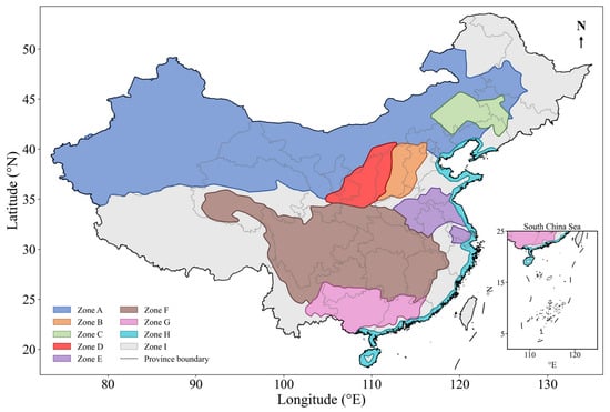
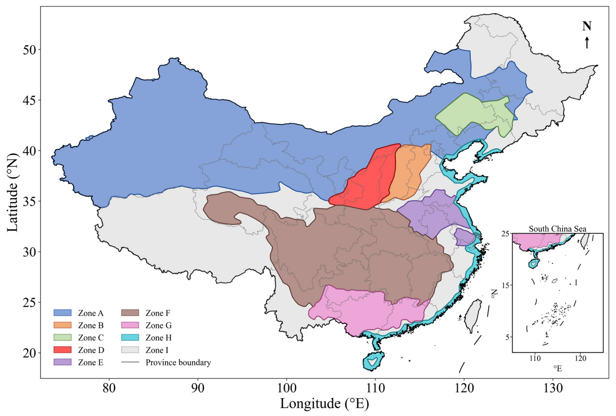
China’s Eight Forestry Engineering Regions include the Three-north shelterbelt program, the Afforestation program for Taihang mountain, the Shelterbelt program for Liaohe River, the Shelterbelt program for middle reaches of Yellow River, the Shelterbelt program for Huaihe River and Taihu lake, the Shelterbelt program for upper and middle reaches of Yangtze River, the Shelterbelt program for Pearl River, and the Coastal shelterbelt program (Figure 1). Together, the eight regions span roughly 675.47 × 10⁴ km2 and extend across about 21°31′–50°9′ N, encompassing a strong hydrothermal gradient that runs from the temperate arid and semi-arid northwest, where sparse grassland and shrubland grow on aridisols, to the warm, humid subtropical southeast, where closed broadleaf and mixed forests grow on acrisols and ferralsols [3,19]. Across this gradient, mean annual precipitation increases from below 100 mm in the northwest to 2400 mm in the southeast [3]. The boundary of the forestry ecological engineering region was acquired from the Resource and Environmental Data Platform.
Figure 1.
Spatial distribution of China’s Eight Forestry Engineering Regions. Zones A–H denote the Three-north shelterbelt program (A), the Afforestation program for Taihang mountain (B), the Shelterbelt program for Liaohe River (C), the Shelterbelt program for middle reaches of Yellow River (D), the Shelterbelt program for Huaihe River and Taihu lake (E), the Shelterbelt program for upper and middle reaches of Yangtze River (F), the Shelterbelt program for Pearl River (G), and the Coastal shelterbelt program (H), respectively. Zone I represents areas outside the Eight Forestry Engineering Regions. Gray lines indicate province boundaries. The inset in the lower right shows the South China Sea region.
2.2. Datasets
Annual NDVI (2001–2025) was derived from the Moderate Resolution Imaging Spectroradiometer (MODIS) MOD13A1 product (500 m resolution) (Raytheon Santa Barbara Remote Sensing (SBRS), Goleta, CA, USA) as the average of valid 16-day composites within each year. Annual NPP (2001–2025) was obtained from the MODIS MOD17A3HGF product at the same resolution [29]. This product is based on a light-use-efficiency model, in which absorbed photosynthetically active radiation—derived from the MODIS FPAR/LAI inputs—is converted to gross primary production using a biome-specific maximum light-use efficiency constrained by daily temperature and vapor pressure deficit, after which maintenance and growth respiration are subtracted to yield annual NPP. All MODIS products were obtained from the NASA Land Atmosphere Near real-time Capability for EOS Distributed Active Archive Center (LAADS DAAC). MOD13A1 and MOD17A3HGF are standard Level-3 products for which radiometric calibration, atmospheric correction, temporal compositing, and geometric registration are implemented during official product generation. No additional pixel-level screening based on the MODIS quality-assurance layers was applied in this study. Annual NDVI was calculated as the mean of the available 16-day MOD13A1 composite values within each year, after excluding NoData values, whereas annual NPP was obtained directly from the MOD17A3HGF annual product. Topographic variables (elevation, slope, sine- and cosine-transformed aspect) were derived from the Shuttle Radar Topography Mission (SRTM) 90 m Digital Elevation Model (DEM) V4.1 product. Multi-year mean annual temperature and total precipitation (2001–2024) were obtained from the 1 km monthly climate datasets for China provided by the National Tibetan Plateau Data Center. Seven soil variables [Soil organic carbon content in the fine earth fraction, soil pH, proportion of clay particles (<0.002 mm) in the fine earth fraction, proportion of sand particles (>0.05 mm) in the fine earth fraction, bulk density of the fine earth fraction, cation exchange capacity of the soil, and total nitrogen] were obtained from SoilGrids (0–30 cm).
All variables used in this study are continuous, and were resampled to a common 500 m grid using bilinear interpolation. Because the analysis targets broad-scale, multi-year average patterns rather than fine local detail, and because most layers were resampled across comparable spatial scales, bilinear interpolation provides a smooth, continuous surface and is well suited to continuous fields, while avoiding the blocky discontinuities of nearest-neighbor assignment. A pixel was treated as valid vegetated if its 25-year mean NDVI exceeded 0.1 and mean NPP exceeded 0 g C m−2 yr−1; all subsequent analyses were restricted to these pixels. Detailed information on the variables, units, sources, native spatial and temporal resolutions, and their roles in the analysis is provided in Table S1.
2.3. Trend Analysis of Vegetation Greenness and Productivity
Pixel-level temporal trends in annual NDVI and NPP from 2001 to 2025 were estimated using the Theil–Sen median slope estimator, and statistical significance was assessed using the Mann–Kendall test (p < 0.05) [30]. The same procedure was applied at the regional scale using annual mean values within each forestry engineering region.
2.4. Sliding-Window Similar-Habitat Model
2.4.1. Estimation of Habitat-Constrained Potentials
A sliding-window similar-habitat model was developed to estimate habitat-constrained vegetation potentials. The current state was calculated as the pixel-wise mean over 2021–2025, and the within-pixel reference layer was defined as the 95th percentile of the 2001–2025 annual time series. Thirteen environmental variables (4 topographic, 2 climatic, and 7 soil) were standardized to z-scores, z = (x − μ)/σ, where μ and σ are the mean and standard deviation of each variable across all valid pixels, so that variables measured in different units contributed comparably to Euclidean distance in environmental space. The climate variables were represented by 2001–2024 multi-year means and, together with terrain and soil, were treated as static habitat descriptors; consequently, the absence of climate data for 2025 did not affect construction of the environmental space. For each focal pixel, a 31 × 31 moving window (approximately 15.5 × 15.5 km at the 500 m grid resolution) was applied. This window was large enough to provide a stable pool of environmentally similar candidates while remaining sufficiently local to limit the inclusion of large climatic or topographic gradients. Euclidean distances to all valid candidates within the window were calculated in the 13-dimensional standardized environmental space. To assess sensitivity to window size, the analysis was repeated using 21 × 21 and 41 × 41 moving windows. The 10% of candidates with the smallest Euclidean distances were selected as similar-habitat pixels, following the original sliding-window similar-habitat approach [24,25,31]. To avoid unstable estimates where a window contained few valid candidates, at least 30 similar-habitat pixels were required, an empirical minimum that stabilized the 95th-percentile reference. The habitat-constrained potential was then estimated as the 95th percentile of the reference values of the selected similar-habitat pixels.
2.4.2. Calculation of Relative Remaining Recovery Potential
The relative remaining recovery potential (RRP) was calculated as:
where values near 0 indicate that the current state has approached its habitat-constrained potential and values near 1 indicate substantial remaining recovery space. The proportion of pixels with RRP > 0.3 within each region was calculated to quantify the spatial extent of high-potential areas.
RRP(i) = 1 − Current(i)/Potential(i), RPP(i) ∈ [0, 1]
2.5. Divergence Analysis Between Greenness and Productivity Recovery Potentials
The pixel-level Pearson and Spearman correlations between NDVI RRP and NPP RRP were calculated within each region and for all regions combined. The two RRP values were paired for the same pixel and then summarized within each spatial unit [21,32]. Four divergence types were defined using an operational threshold of 0.3 to distinguish pixels that had reached more than 70% of their estimated habitat-constrained potential (RRP < 0.3) from those retaining appreciable remaining recovery space (RRP ≥ 0.3): Type I (low NDVI RRP and low NPP RRP), Type II (high NDVI RRP and high NPP RRP), Type III (low NDVI RRP and high NPP RRP), and Type IV (high NDVI RRP and low NPP RRP). The threshold was used only to summarize spatial extent and classify divergence types, not as a model parameter; its influence on the type proportions was tested at 0.25, 0.30, and 0.35. All analyses were performed in Python 3.7, using NumPy and pandas for data processing, GDAL and geopandas for geospatial operations, and SciPy for statistical analyses.
2.6. Robustness to Spatial Autocorrelation
Because the pixel-level correlation analysis involves a very large number of grid cells (≈22.7 million valid vegetated pixels), conventional significance tests are strongly affected by spatial autocorrelation, which inflates the effective number of independent observations and renders p-values uninformative. To assess whether the estimated NDVI-RRP–NPP-RRP correlations are robust to this spatial dependence, we performed a spatial subsampling analysis together with an effective-sample-size correction.
For each region (and for all regions combined), the spatial autocorrelation range of the NDVI-RRP and NPP-RRP fields was first estimated from their empirical semivariograms, computed on 2 × 10⁵ randomly selected pixel pairs. To prevent large-scale spatial trends (e.g., the southeast–northwest gradient) from being mistaken for short-range autocorrelation, the maximum lag was capped at a physically plausible bound (50 km) and the sill was estimated from the stable upper portion of the semivariogram. Pixel coordinates were projected to an Albers equal-area projection so that all distances were computed in meters.
We then drew 1000 spatially independent subsamples in which no two retained pixels were closer than the estimated autocorrelation range, and recomputed the Pearson and Spearman correlations on each subsample. The mean correlation and its 2.5th–97.5th percentile interval are reported. For the eight-region pooled analysis, subsampling was performed within each region separately and the independent samples were then combined, to avoid the inter-regional gaps of the spatially disjoint engineering regions being treated as part of a single continuous field. Finally, an effective sample size (n_eff) was approximated from the autocorrelation patch area, and the significance of each full-sample correlation was re-evaluated using n_eff in place of the pixel count. A correlation was regarded as robust only if its sign and approximate magnitude were preserved across subsamples and it remained significant after the effective-sample-size correction. All computations were performed in Python 3.11.
To evaluate whether relatively low linear correlations reflected nonlinear dependence, we additionally compared linear regression with locally weighted scatterplot smoothing (LOWESS) in the three regions with the lowest full-sample Pearson correlations (Zones B, G, and H). For each region, the comparison used a reproducible spatially thinned sample based on the estimated autocorrelation range, followed by 30 repeated random train-test splits with 20% of observations retained for testing. Predictive performance on the held-out samples was evaluated using the coefficient of determination (R2), root mean square error (RMSE), and mean absolute error (MAE). This exploratory analysis assessed nonlinear curve shape and descriptive adequacy rather than causal effects.
3. Results
3.1. Temporal and Spatial Changes in Vegetation Greenness and Productivity
3.1.1. Regional Temporal Trends in NDVI and NPP
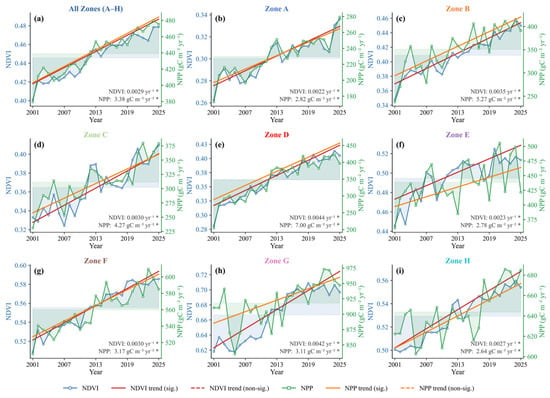
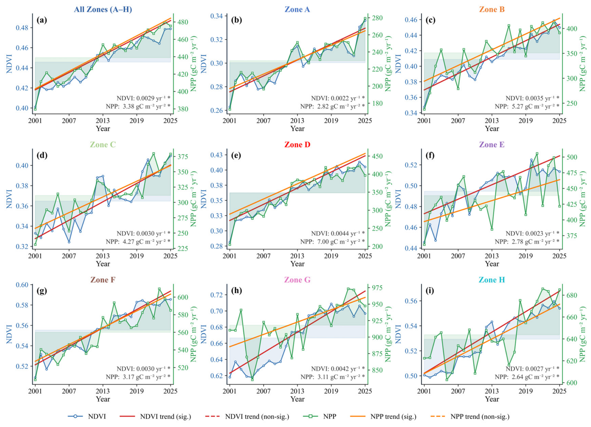
From 2001 to 2025, both NDVI and NPP displayed significant upward trends across China’s Eight Forestry Engineering Regions (p < 0.05; Figure 2). The overall annual mean NDVI increased at 0.0029 yr−1 and NPP at 3.38 g C m−2 yr−1 per year (Figure 2a). Substantial differences were observed among regions: the middle Yellow River shelterbelt region showed the strongest increasing trends, with NDVI and NPP increasing at 0.0044 yr−1 and 7.00 g C m−2 yr−1 per year, respectively (Figure 2e), while the Three-north shelterbelt program and the Coastal shelterbelt program showed the weakest greenness and productivity trends, respectively (Figure 2b,i).
Figure 2.
Interannual changes in vegetation greenness and productivity across China’s Eight Forestry Engineering Regions from 2001 to 2025. Panels show annual mean NDVI and NPP for all forestry engineering regions combined (a) and for individual regions Zones A–H (b–i), as defined in Figure 1. Blue lines represent NDVI, and green lines represent NPP. Shaded bands represent annual deviations from the 2001–2025 multi-year mean. Red and orange lines indicate fitted trends for NDVI and NPP, respectively. Slope values are shown in each panel, with an asterisk (*) indicating a statistically significant slope at p < 0.05.
3.1.2. Pixel-Level Spatial Trends in NDVI and NPP
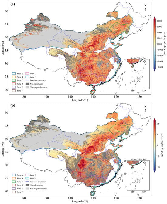
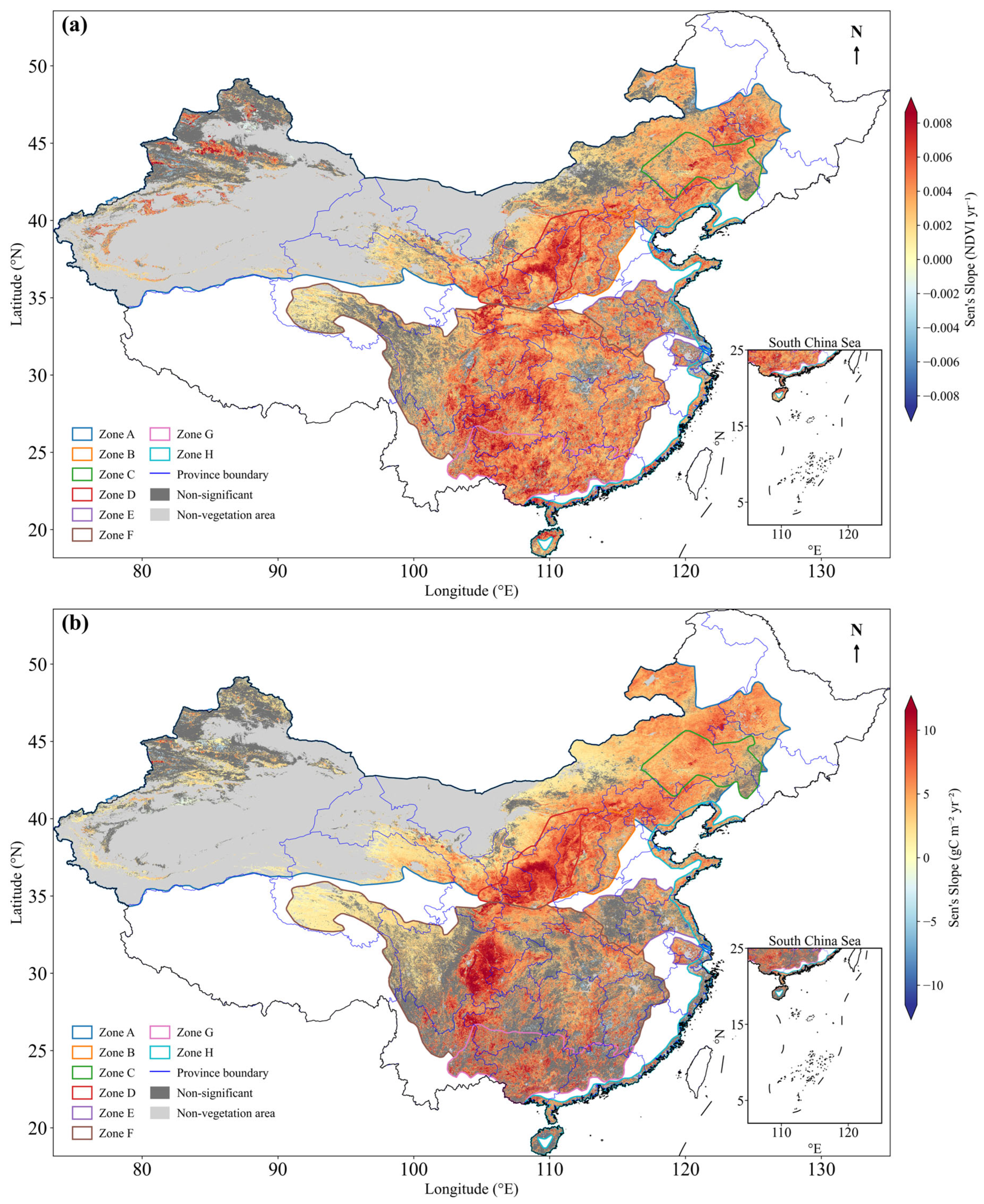
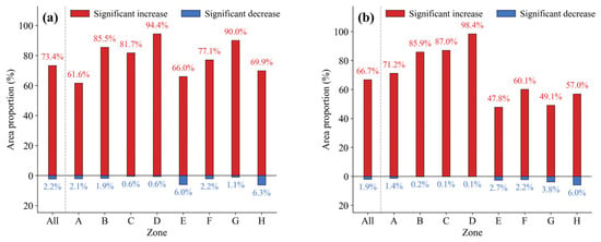
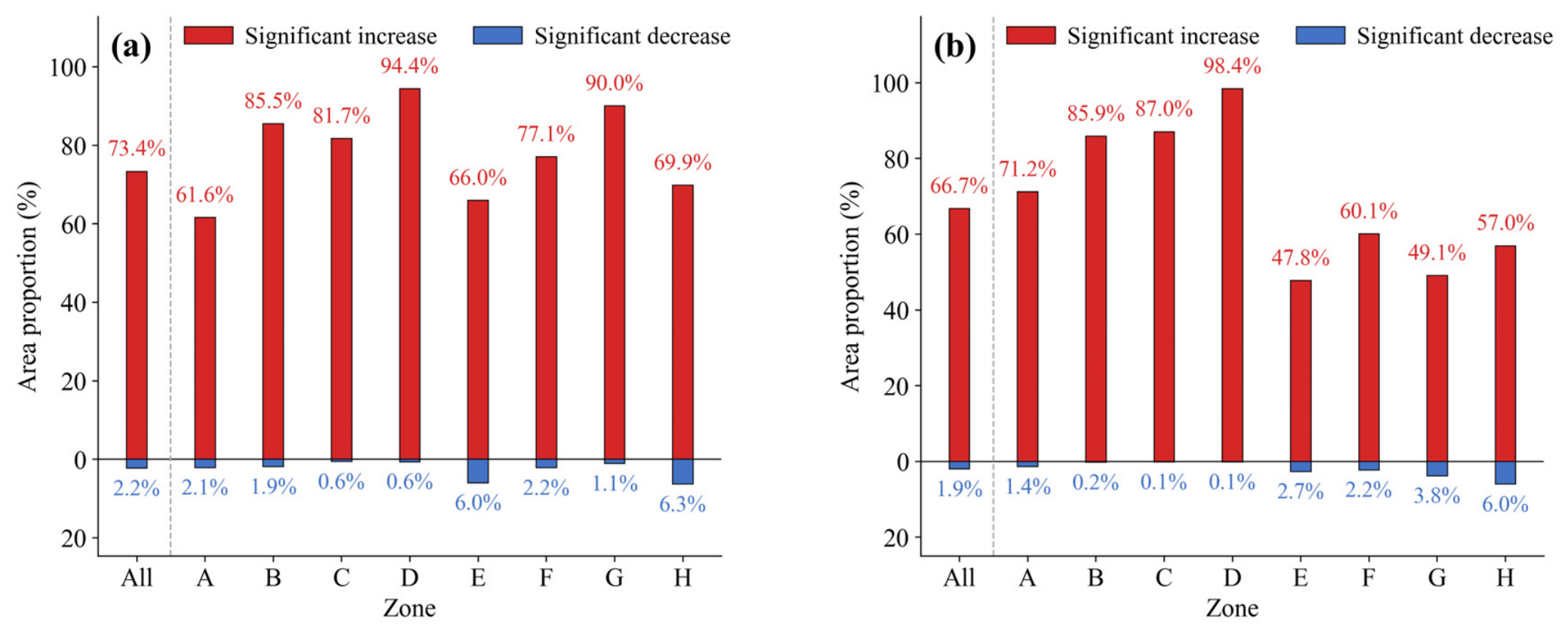
Pixel-level analysis revealed pronounced spatial heterogeneity within and across regions, with the strongest NDVI and NPP increases concentrated in the middle and lower Yellow River, upper Yangtze River, and Pearl River basin (Figure 3a,b). Significant decreasing trends were detected in parts of southeastern China and along the eastern coast, but their spatial extent was limited compared with areas of significant increase. Across all regions, 73.4% and 66.7% of the valid vegetated area showed significant NDVI and NPP increases, respectively, while only 2.2% and 1.9% experienced significant decreases. The remaining 24.4% (NDVI) and 31.4% (NPP) showed no significant trend (Figure 4a,b). The shelterbelt program for the middle reaches of the Yellow River contained the largest proportions of significantly increasing pixels, reaching 94.4% for NDVI and 98.4% for NPP. By contrast, the Three-north shelterbelt program had the lowest proportion of significant NDVI increase, whereas the Coastal shelterbelt program showed a relatively low proportion of significant NPP increase, further highlighting regional divergence between greenness and productivity trends.
Figure 3.
Spatial patterns of pixel-level trends in vegetation greenness and productivity across China’s Eight Forestry Engineering Regions from 2001 to 2025. Panels show the spatial distribution of Sen’s slope for NDVI (a) and NPP (b), with colored pixels representing trends that are statistically significant (p < 0.05). Dark gray indicates pixels with non-significant trends, and light gray indicates non-vegetation areas. Colored lines represent the boundaries of the Eight Forestry Engineering Regions, and blue lines denote province boundaries. The insets in the lower right show the South China Sea region.
Figure 4.
Proportions of valid vegetated area with statistically significant trends in NDVI (a) and NPP (b) across China’s Eight Forestry Engineering Regions from 2001 to 2025. Red bars indicate the proportion of pixels with significant increases, and blue bars indicate the proportion of pixels with significant decreases (p < 0.05). “All” represents all forestry engineering regions combined, and Zones A–H are defined in Figure 1. Values above and below the bars show the corresponding area proportions.
3.2. Habitat-Constrained Vegetation Potentials and Remaining Recovery Potentials
3.2.1. Spatial Patterns of Habitat-Constrained Potentials
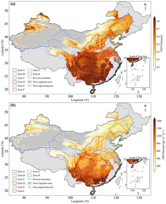
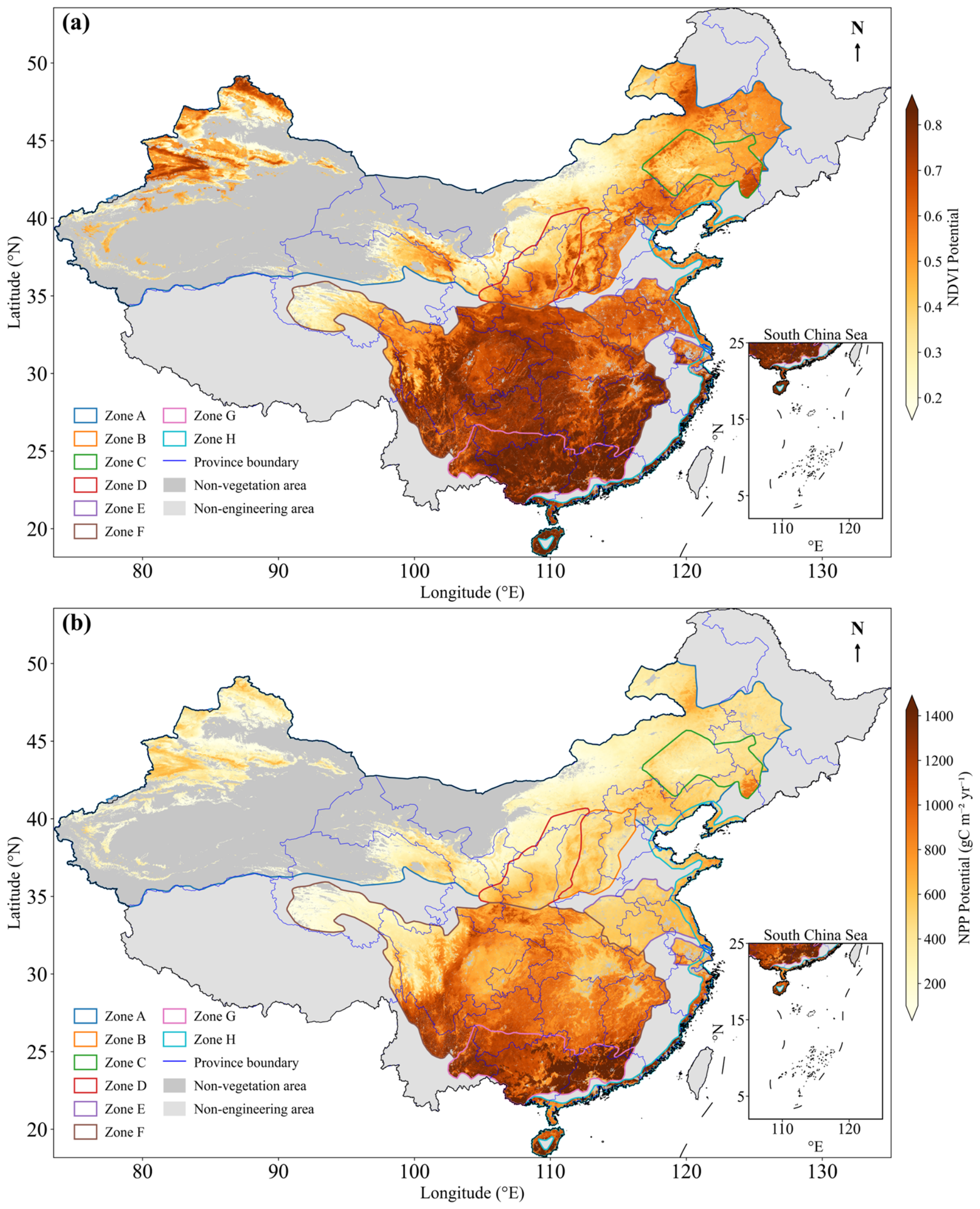
The habitat-constrained NDVI and NPP potentials displayed a general southeast-to-northwest decreasing gradient, with the Pearl River shelterbelt program reaching the highest values (NDVI: 0.79; NPP: 1234.38 g C m−2 yr−1) and the Three-north shelterbelt program the lowest (NDVI: 0.38; NPP: 318.54 g C m−2 yr−1; Table 1; Figure 5). This gradient was consistent for both indicators, although the spatial contrast in NPP potential was more pronounced than that in NDVI potential. Regions located in southern and southeastern China generally showed higher current and potential values, whereas northern and northwestern regions showed lower values for both greenness and productivity.
Table 1.
Summary of vegetation greenness (NDVI) and productivity (NPP) recovery indicators across China’s Eight Forestry Engineering Regions.
Figure 5.
Spatial patterns of habitat-constrained NDVI potential (a) and NPP potential (b) across China’s Eight Forestry Engineering Regions, estimated using the sliding-window similar-habitat model. Dark gray indicates non-vegetation areas, and light gray indicates areas outside the Eight Forestry Engineering Regions. Colored lines represent Zones A–H, as defined in Figure 1, and blue lines denote province boundaries. The insets in the lower right show the South China Sea region.
3.2.2. Relative Remaining Recovery Potentials and Their Robustness
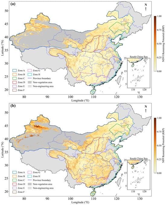
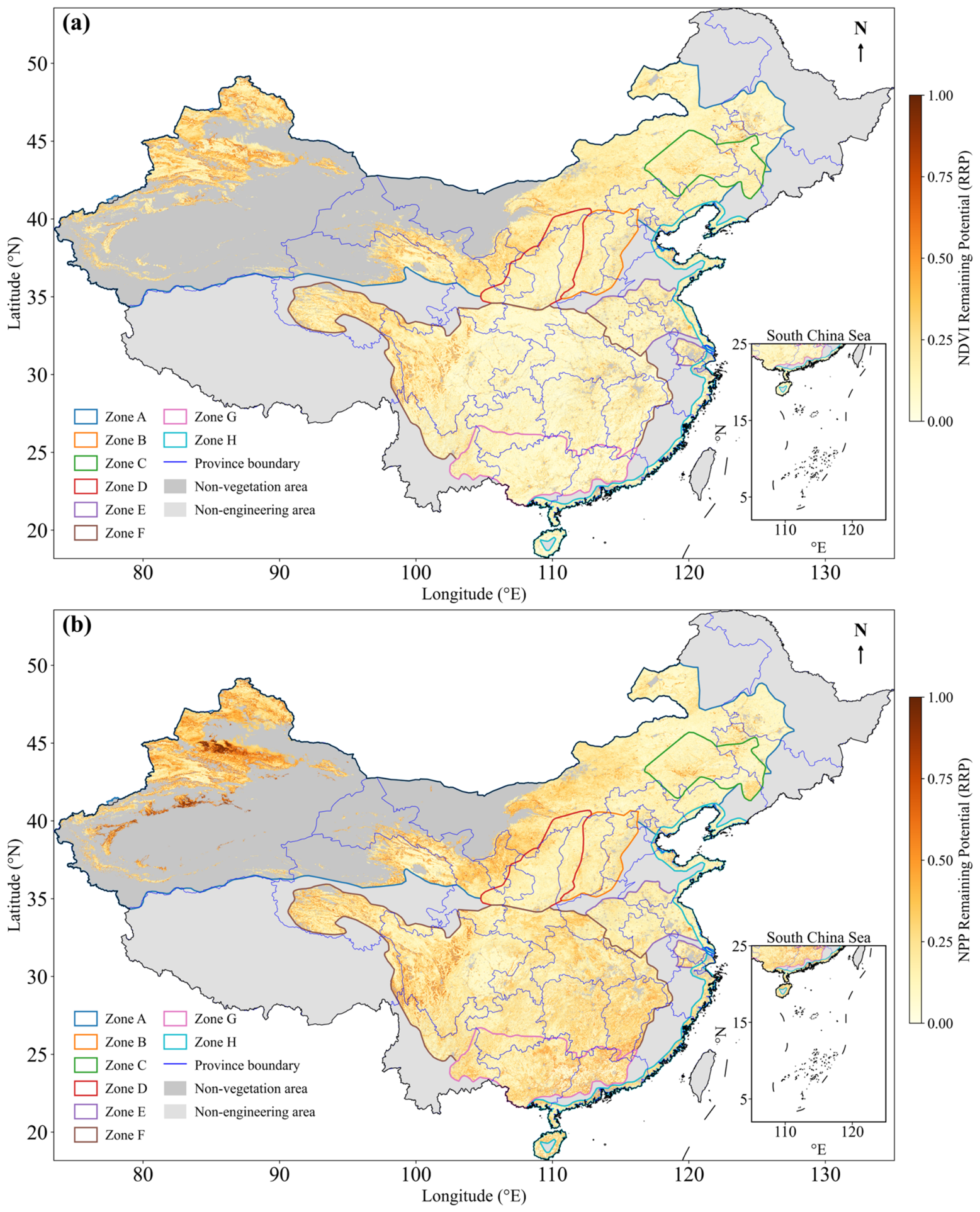
RRP values across the eight regions were generally low: NDVI RRP ranged from 0.09 to 0.21 and NPP RRP from 0.16 to 0.25, indicating that most areas have already approached their habitat-constrained potentials (Table 1; Figure 6). Higher RRP values were concentrated in parts of the Three-north shelterbelt program, particularly in northern Xinjiang and the western Inner Mongolia plateau. For most regions, NPP RRP was higher than NDVI RRP, indicating that productivity generally retained more remaining recovery space than greenness. The proportion of pixels with RRP > 0.3 ranged from 1.9% in the Pearl River shelterbelt program for NDVI to 31.1% in the Three-north shelterbelt program for NPP, and exceeded 20% in five of the eight regions for NPP (Table 1). In contrast, high NDVI RRP areas were more spatially restricted, suggesting that greenness recovery was closer to its habitat-constrained potential than productivity recovery in many regions.
Figure 6.
Spatial patterns of relative remaining recovery potential (RRP) of NDVI (a) and NPP (b) across China’s Eight Forestry Engineering Regions. Dark gray indicates non-vegetation areas, and light gray indicates areas outside the Eight Forestry Engineering Regions. Colored lines represent Zones A–H, as defined in Figure 1, and blue lines denote province boundaries. The insets in the lower right show the South China Sea region.
To evaluate the robustness of our habitat-constrained potential estimates, we compared RRP values derived from three sliding-window sizes: 21 × 21, 31 × 31, and 41 × 41. Across all eight regions, the mean NDVI RRP varied by less than 0.03 (absolute difference between the smallest and largest window), and the mean NPP RRP varied by less than 0.04 (Table S2). The corresponding spatial patterns also remained highly consistent across window sizes (Figure S1). These results indicate that our main conclusions—particularly the low RRP in most regions and the divergence between greenness and productivity recovery potentials—are moderately robust to the choice of window size, with larger windows tending to produce slightly higher RRP estimates.
3.3. Divergence Between Greenness and Productivity Recovery Potentials
3.3.1. Correlation and Nonlinear Relationships Between NDVI and NPP RRP
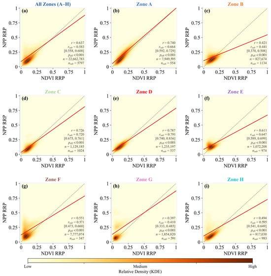
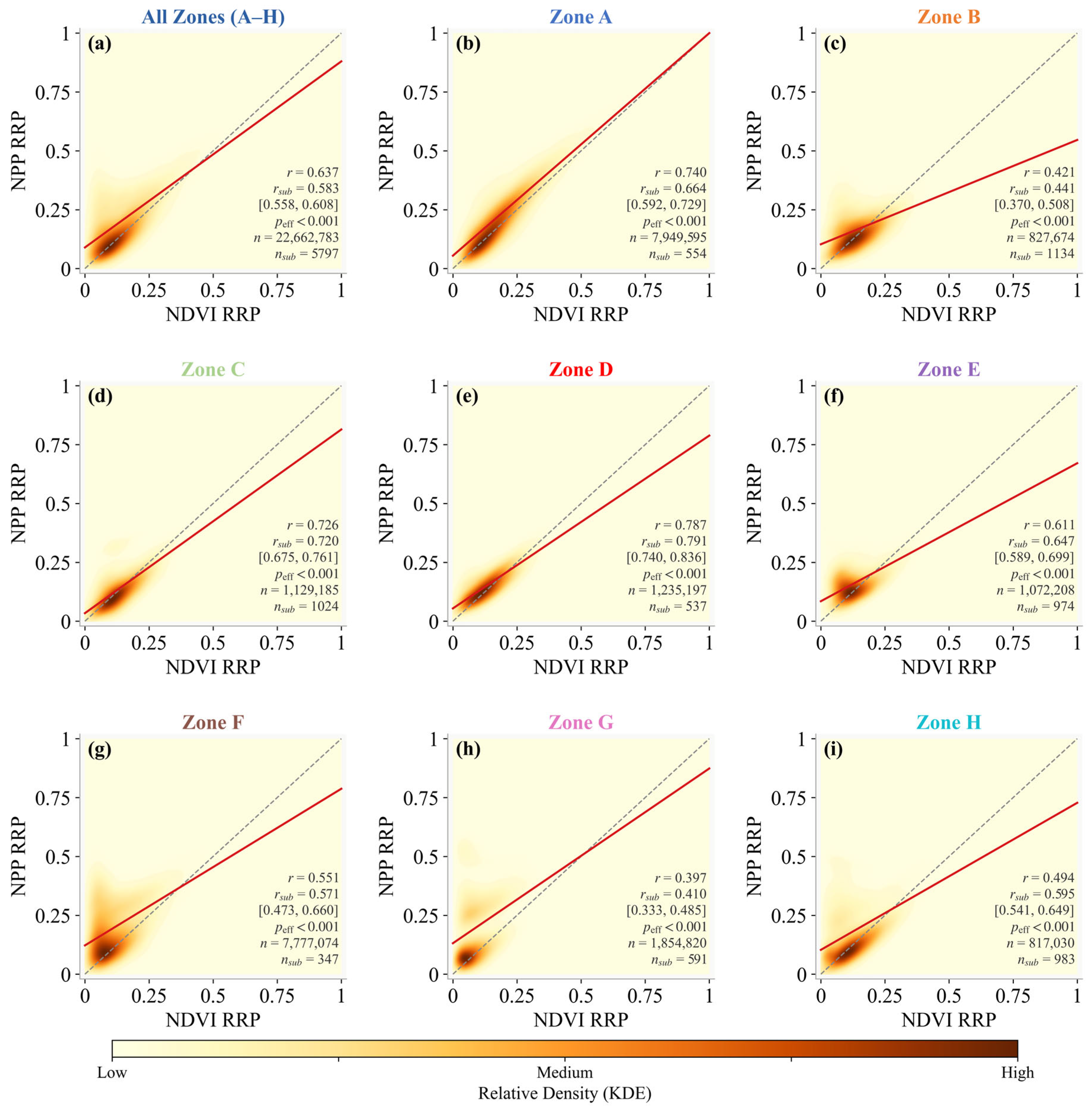
NDVI RRP and NPP RRP were positively correlated across all regions (overall Pearson r = 0.637; Figure 7a), with correlation strength varying substantially among regions, from r = 0.79 in the middle Yellow River shelterbelt program (Zone D) to r = 0.40 in the Pearl River shelterbelt program (Zone G). Because the pixel count is very large, we assessed these correlations using spatial subsampling and an effective-sample-size correction rather than relying on p-values (Section 2.6; Table S3). The subsample-based correlations closely reproduced the full-sample values (overall mean r = 0.583, 95% CI 0.558–0.608) and preserved the regional ranking, and all correlations remained significant after correcting for spatial autocorrelation (n_eff = 312–5341; p < 0.001). NPP RRP was consistently higher than NDVI RRP across all regions, as indicated by the regression lines lying below the 1:1 line in all panels. This pattern suggests that greenness-based recovery potential does not fully represent productivity-based recovery potential.
Figure 7.
Comparison of remaining greenness and productivity recovery potentials at the pixel scale. Panels show the relationship between NDVI relative remaining recovery potential (RRP) and NPP RRP for all forestry engineering regions combined (a) and for Zones A–H (b–i). Colors indicate the relative density of pixels estimated by kernel density estimation. The gray dashed line represents the 1:1 line, and the red line represents the fitted linear regression. Each panel shows the full-sample Pearson correlation (r), the mean correlation from 1000 spatially independent subsamples (r_sub) with its 95% confidence interval, and the number of pixels (n). Significance was assessed after an effective-sample-size correction for spatial autocorrelation (Section 2.6; Table S3); all correlations remained significant (p < 0.001). Zones A–H are defined in Figure 1.
The robustness of the RRP estimates to sliding-window size was further supported by the high-RRP area statistics. Although the proportions of pixels with high RRP (>0.3) varied slightly among the 21 × 21, 31 × 31, and 41 × 41 windows, the regional rankings remained highly consistent, with larger windows generally yielding somewhat higher proportions (Table S4).
Exploratory nonlinear comparisons provided little evidence that the relatively weak correlations in Zones B, G, and H were primarily caused by strong nonlinear dependence. LOWESS increased the mean held-out R2 from 0.211 to 0.258 in Zone B and from 0.358 to 0.387 in Zone H, but the corresponding reductions in RMSE were only 3.2% and 2.3%, respectively. In Zone G, LOWESS performed slightly worse than the linear model (R2 = 0.120 versus 0.129). The linear fits therefore remained adequate descriptive summaries, while the lower correlations mainly indicated incomplete coupling between greenness- and productivity-based recovery potentials (Figure S2).
3.3.2. Spatial Patterns of Greenness–Productivity Divergence Types
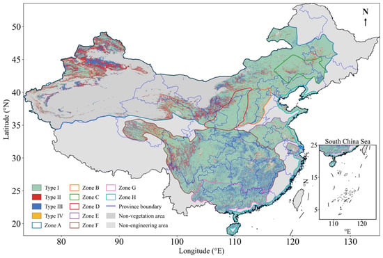
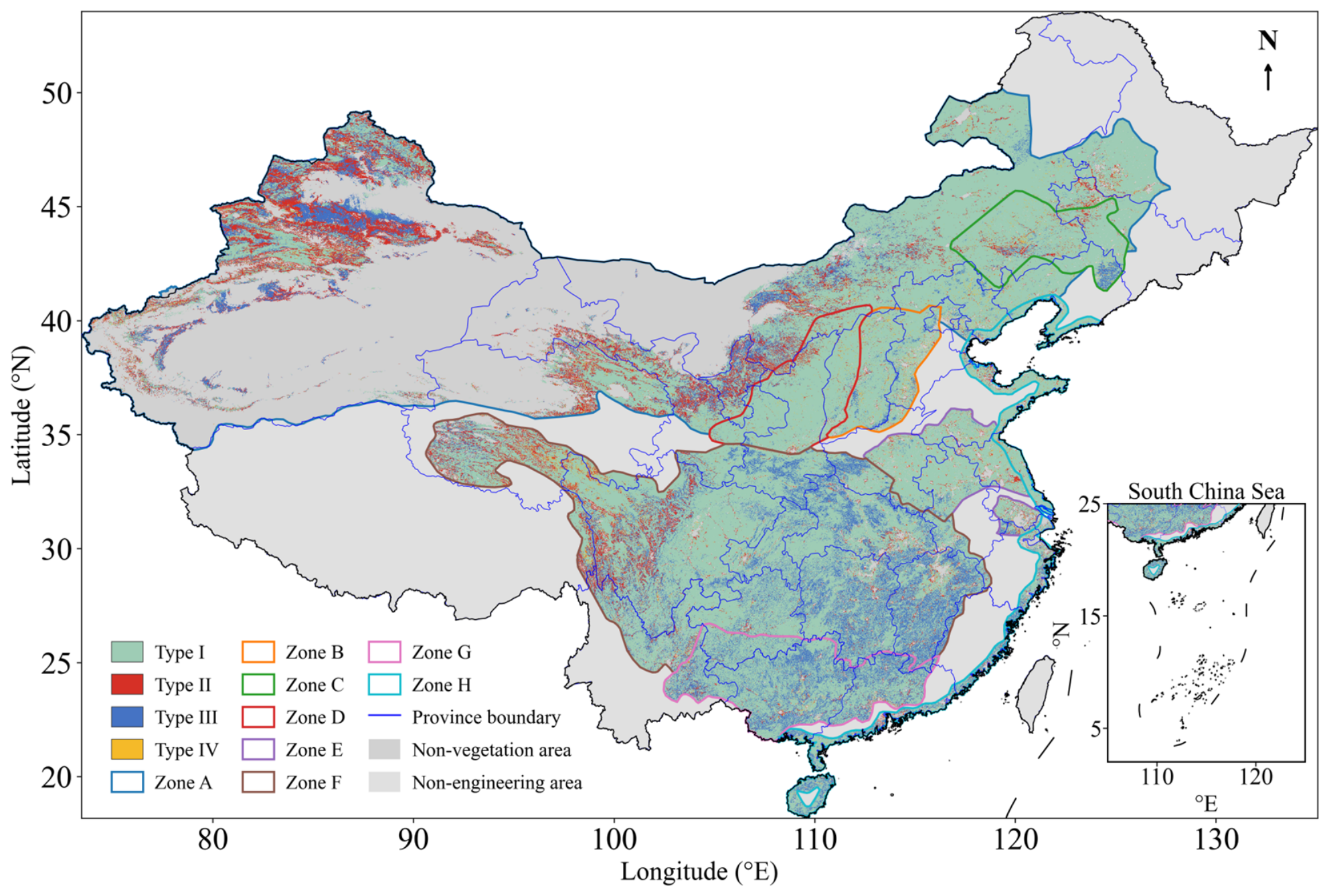
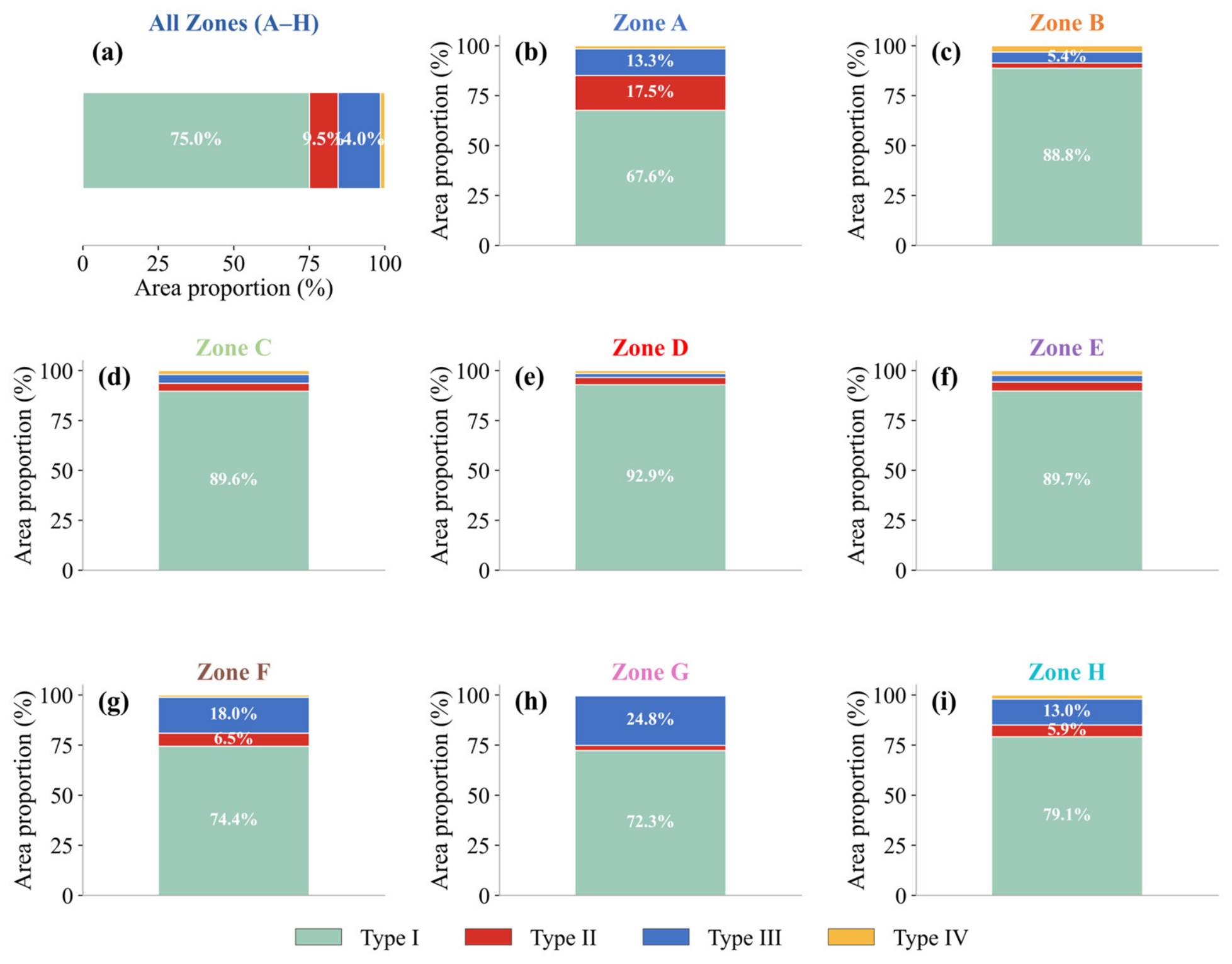
Based on the four divergence types, Type I (low NDVI RRP and low NPP RRP) dominated most regions, accounting for 75.0% of the valid vegetated area, and was widely distributed across southern China, the Yangtze River basin, and the Pearl River basin (Figure 8 and Figure 9a). Type III (low NDVI RRP and high NPP RRP) accounted for 14.0%, Type II (high NDVI RRP and high NPP RRP) for 9.5%, and Type IV (high NDVI RRP and low NPP RRP) for only 1.5%. Spatially, Type II areas were mainly concentrated in northern Xinjiang and western Inner Mongolia, overlapping with zones of relatively high RRP for both indicators. Type III areas were more widely scattered across central, southern, and coastal regions, suggesting that some areas with limited greenness remaining potential may still retain considerable productivity remaining potential. At the regional scale, the middle Yellow River shelterbelt program had the highest Type I proportion (92.9%), while the Pearl River shelterbelt program had the largest Type III proportion (24.8%; Figure 9b–i). This regional contrast further indicates that the degree of coupling between greenness and productivity recovery potentials differs markedly among forestry engineering regions.
Figure 8.
Divergence types between greenness recovery potential and productivity recovery potential. Four types are defined based on the combination of NDVI RRP and NPP RRP using a fixed threshold of 0.3 (values < 0.3 classified as low and values ≥ 0.3 as high): Type I (low NDVI RRP and low NPP RRP), Type II (high NDVI RRP and high NPP RRP), Type III (low NDVI RRP and high NPP RRP), and Type IV (high NDVI RRP and low NPP RRP). Dark gray indicates non-vegetation areas, and light gray indicates areas outside the Eight Forestry Engineering Regions. Black lines denote the boundaries of the Eight Forestry Engineering Regions, and blue lines denote province boundaries. The inset in the lower right shows the South China Sea region.
Figure 9.
Area proportions of the four divergence types between NDVI and NPP relative remaining recovery potentials (RRP) across China’s Eight Forestry Engineering Regions. Panels show the area proportions for all forestry engineering regions combined (a) and for Zones A–H (b–i), with the four types defined as in Figure 8. Values inside the bars indicate the area proportions of the dominant types. Zones A–H are defined in Figure 1.
The four-type classification was robust to reasonable variation in the RRP threshold. Across thresholds of 0.25–0.35, Type I remained dominant for all zones combined (64.2%–83.7%), Type III remained the second-largest type (9.4%–18.4%), and Type IV remained marginal at the overall scale (0.8%–2.6%). The broad regional contrast was also preserved, with Zone D consistently showing the highest Type I proportion and Zone G consistently showing the highest Type III proportion (Table S5).
4. Discussion
Our results demonstrate widespread but spatially heterogeneous increases in vegetation greenness and productivity across China’s Eight Forestry Engineering Regions during 2001–2025, consistent with increasing evidence that China has been a major contributor to global vegetation greening in association with sustained land-use management, afforestation, and ecological restoration [7,17]. Recent national-scale studies have suggested an important contribution of ecological restoration programs to vegetation greening, while also emphasizing that observed greening patterns vary substantially among regions and are strongly mediated by local climate conditions [33,34]. Among the eight regions, the middle Yellow River shelterbelt region showed the strongest increases in both NDVI and NPP, a pattern that is spatially consistent with long-term soil and water conservation measures and large-scale vegetation restoration under the Grain for Green Program on the Loess Plateau [35]. By contrast, the weaker greenness increase in the Three-north shelterbelt region and the relatively weak productivity increase in the Coastal shelterbelt region suggest that observed recovery patterns may be constrained by regional water availability, background vegetation type, and climatic variability. This regional divergence is consistent with recent studies showing that forestry engineering regions often exhibit enhanced greenness, whereas productivity may remain more sensitive to climate stress and environmental constraints [3,36].
The habitat-constrained potentials estimated by the sliding-window similar-habitat model provide ecologically meaningful benchmarks by comparing each pixel with environmentally comparable reference pixels within local neighborhoods, thereby reducing the risk of overestimating recovery potential in arid habitats or underestimating it in humid areas [25,31]. The generally low RRP values across most regions suggest that current vegetation states are close to their estimated habitat-constrained reference levels in many areas, implying that further gains from vegetation-cover expansion alone may be limited in these locations. These results suggest that restoration assessment and management in such areas may need to shift from an emphasis on continued area expansion toward maintaining existing vegetation gains, improving ecosystem quality, and enhancing long-term stability [37]. Nevertheless, high RRP values in parts of the Three-north shelterbelt region, northern Xinjiang, and mountainous transition zones indicate remaining vegetation recovery potential, although these areas are often water-limited or ecotonal environments where further restoration planning should be carefully balanced against hydrological sustainability. Previous studies have shown that large-scale vegetation restoration in drylands can exceed local water carrying capacity and increase the risk of hydrological unsustainability [38,39,40].
A key finding is that greenness and productivity recovery potentials were positively correlated but not fully synchronized, a relationship that remained robust under spatial subsampling and an effective-sample-size correction. NPP RRP was generally higher than NDVI RRP, suggesting that productivity still retains greater remaining recovery space than greenness in many areas. This divergence is ecologically important because NDVI primarily reflects canopy structure and vegetation cover, whereas NPP integrates photosynthetic carbon assimilation and is more directly linked to ecosystem functional performance. The mismatch has been reported in recent global and regional studies showing that increasing greenness does not necessarily translate into proportional increases in NPP, resilience, or ecosystem functioning [19,21,32]. In our study, Type III areas accounted for 14.0% of the valid vegetated area, suggesting that a substantial fraction was close to its estimated greenness reference state while retaining considerable productivity remaining potential. Several possible explanations may account for this pattern. NDVI can saturate in dense canopies, whereas productivity may continue to respond to canopy photosynthetic efficiency, stand age, and nutrient availability. In addition, climate variability and extreme events may weaken productivity gains even where greenness continues to increase [16]. These findings suggest that greenness-based assessments alone may overestimate functional recovery in some areas, particularly where canopy structural recovery and productivity recovery are decoupled.
The nonlinear comparison also cautions against attributing weak greenness–productivity coupling solely to regression curvature or NDVI saturation. Zone G showed no improvement under LOWESS, whereas the modest improvements in Zones B and H had little practical effect on prediction error. NDVI saturation therefore remains a plausible ecological mechanism, together with stand age, species composition, nutrient status, and climate variability, but cannot be confirmed from the regression form alone.
The four divergence types provide a practical basis for differentiated restoration assessment and spatial prioritization. Type I areas were close to both estimated greenness and productivity reference states. These areas may be more suitable for conservation and maintenance of existing vegetation gains than for further vegetation expansion. Type II areas, where both structural and functional recovery potentials remain high, may represent potential priority zones for future restoration assessment and planning, but site-specific strategies based on water availability, soil conditions, and long-term sustainability are needed to avoid uniform afforestation targets. Type III areas showed low NDVI RRP but high NPP RRP, indicating relatively limited greenness remaining potential but greater productivity remaining potential. In these areas, restoration planning may need to focus less on increasing canopy cover alone and more on improving ecosystem function through stand quality improvement, mixed-species planting, and adaptive forest management, while considering potential biodiversity co-benefits [41]. Type IV areas require careful local diagnosis before intervention. Overall, our results are consistent with a transition from quantity-oriented afforestation assessment toward quality-oriented ecosystem monitoring and management, in line with recent studies emphasizing that forest restoration planning should better match species selection, timing, and management intensity to regional ecological constraints rather than simply expanding planted area [9,10,42].
Several uncertainties should be acknowledged. First, the 500 m resolution of the MODIS products inherently obscures small-scale conservation measures, community woodlots, fragmented patches, and localized management interventions. Resampling higher-resolution terrain, soil, and climate layers to this grid may further smooth local extrema that help explain fine-scale NPP variation. Second, uncertainties in the MOD17 NPP product arise from climate inputs, light-use-efficiency parameterization, and land-cover classification, and the absence of plot- or flux-tower validation limits direct confirmation of the inferred greenness–productivity mismatches. Third, the habitat-constrained potential represents an attainable state under current environmental conditions and should not be interpreted as an absolute maximum under future climate change or intensive intervention. Although sensitivity analyses indicated that the principal patterns were robust to window size and the RRP threshold, the estimates still depend on the selected environmental variables and reference definition. Fourth, environmental similarity does not guarantee ecological similarity. Pixels with comparable terrain, climate, and soil may differ in stand age, species composition, vertical canopy structure, and management history; consequently, RRP represents remaining space in structural or functional intensity rather than a complete measure of ecosystem quality or integrity. Future work should integrate forest inventory, species-composition, LiDAR, and field-observation data [43,44]. Finally, because this study did not employ a formal counterfactual design, the observed trends should be interpreted as coinciding with, rather than as direct causal effects of, forestry engineering programs. Without matched controls, the management signal cannot be cleanly separated from concurrent climate trends, CO2 fertilization, natural succession, and land-use change. Future studies should integrate matched control pixels, Before–After–Control–Impact designs, or difference-in-differences approaches.
5. Conclusions
This study provides a systematic, dual-indicator remote-sensing assessment of vegetation greenness and productivity recovery status and remaining recovery potential within China’s Eight Forestry Engineering Regions from 2001 to 2025. Both NDVI and NPP increased significantly across all regions, yet their increasing rates diverged markedly: the middle Yellow River shelterbelt region exhibited the strongest NDVI and NPP increases, whereas the Three-north and Coastal shelterbelt regions showed relatively weaker responses. The sliding-window similar-habitat model suggested that many regions were close to their estimated habitat-constrained reference states, with low relative remaining recovery potential (RRP) prevailing across the majority of valid vegetated areas; high RRP persisted primarily in water-limited and ecotonal zones where further restoration planning should consider hydrological carrying-capacity constraints. A central finding is that greenness and productivity recovery potentials were positively but imperfectly correlated, and 14.0% of the valid vegetated area exhibited low greenness RRP alongside high NPP RRP, indicating that canopy structural recovery does not necessarily imply equivalent functional productivity recovery. The four-type divergence classification—in which Type I areas are more suitable for conservation-oriented maintenance, Type III areas may require quality-oriented functional improvement, and Type II areas may represent candidate zones for ecologically informed and water-aware restoration planning—provides a practical framework for differentiated restoration assessment and spatial prioritization within China’s large-scale forestry engineering regions. This dual-indicator approach is also relevant to remote-sensing-based monitoring and evaluation of large-scale ecological restoration initiatives.
Supplementary Materials
The following supporting information can be downloaded at: https://www.mdpi.com/article/10.3390/f17070813/s1, Figure S1: Spatial patterns of NDVI and NPP relative remaining recovery potential (RRP) estimated using different sliding-window sizes; Figure S2: Comparison of linear and nonlinear relationships between NDVI and NPP relative remaining recovery potentials in the three regions with the lowest full-sample correlations; Table S1: Summary of datasets and variables used in this study; Table S2: Regional mean NDVI and NPP relative remaining recovery potential (RRP) under different sliding-window sizes; Table S3: Robustness of the NDVI-RRP versus NPP-RRP correlation to spatial autocorrelation; Table S4: Proportion of high-RRP pixels under different sliding-window sizes; Table S5: Sensitivity of the four divergence-type area proportions to the RRP threshold.
Author Contributions
All authors contributed to the present paper’s preparation. Methodology, P.W. and J.C.; validation, S.M.; data curation, J.Y., H.S. and J.Z.; writing—original draft preparation, P.W.; writing—review and editing, J.Z. All authors have read and agreed to the published version of the manuscript.
Funding
This research is supported by the National Natural Science Foundation of China (42401367, 42505166), the Natural Science Foundation of Shandong Province (ZR2025QC361), the Taishan Scholars Program for Young Experts of Shandong Province (tsqn202507266), and the Project of Young Innovation Team in the Universities of Shandong Province (STKF201926).
Data Availability Statement
The NDVI dataset can be sourced from https://ladsweb.modaps.eosdis.nasa.gov/search/order/1/MOD13A1--61 (accessed on 15 May 2026). The NPP product can be accessed at https://ladsweb.modaps.eosdis.nasa.gov/search/order/1/MOD17A3HGF--61 (accessed on 18 May 2026). The temperature product can be accessed at https://data.tpdc.ac.cn/en/data/71ab4677-b66c-4fd1-a004-b2a541c4d5bf/ (accessed on 15 May 2026). The precipitation dataset was obtained from https://data.tpdc.ac.cn/en/data/faae7605-a0f2-4d18-b28f-5cee413766a2/ (accessed on 19 May 2026). The SRTM 90m DEM V4.1 data can be accessed at https://srtm.csi.cgiar.org/srtmdata/ (accessed on 20 May 2026). The SoilGrids dataset can be sourced from https://isric.org/explore/soilgrids (accessed on 20 May 2026). The boundary of forestry ecological engineering region can be accessed at https://www.resdc.cn/data.aspx?DATAID=138 (accessed on 20 May 2026).
Conflicts of Interest
The authors declare no conflicts of interest.
References
- Baker, D.J.; Gaston, K.J.; Metcalfe, K.; Maclean, I.M.D. Systematic conservation planning for nature recovery. BioScience 2025, 75, 472–489. [Google Scholar] [CrossRef] [Scilit] [PubMed]
- Fu, B.; Liu, Y.; Meadows, M.E. Ecological restoration for sustainable development in China. Natl. Sci. Rev. 2023, 10, nwad033. [Google Scholar] [CrossRef] [Scilit] [PubMed]
- Liu, H.; Wang, Z.; Wang, Z.; Zeng, Y.; Xue, P.; Zhang, M. Stability of the ecosystem gross primary productivity increasing in Chinese forestry ecological engineering area. Agric. Ecosyst. Environ. 2023, 356, 108636. [Google Scholar] [CrossRef] [Scilit]
- Bryan, B.A.; Gao, L.; Ye, Y.; Sun, X.; Connor, J.D.; Crossman, N.D.; Stafford-Smith, M.; Wu, J.; He, C.; Yu, D.; et al. China’s response to a national land-system sustainability emergency. Nature 2018, 559, 193–204. [Google Scholar] [CrossRef] [Scilit] [PubMed]
- Chen, C.; Park, T.; Wang, X.; Piao, S.; Xu, B.; Chaturvedi, R.K.; Fuchs, R.; Brovkin, V.; Ciais, P.; Fensholt, R.; et al. China and India lead in greening of the world through land-use management. Nat. Sustain. 2019, 2, 122–129. [Google Scholar] [CrossRef] [Scilit] [PubMed]
- Zhu, Z.; Piao, S.; Myneni, R.B.; Huang, M.; Zeng, Z.; Canadell, J.G.; Ciais, P.; Sitch, S.; Friedlingstein, P.; Arneth, A.; et al. Greening of the Earth and its drivers. Nat. Clim. Change 2016, 6, 791–795. [Google Scholar] [CrossRef] [Scilit]
- Piao, S.; Wang, X.; Park, T.; Chen, C.; Lian, X.; He, Y.; Bjerke, J.W.; Chen, A.; Ciais, P.; Tømmervik, H.; et al. Characteristics, drivers and feedbacks of global greening. Nat. Rev. Earth Environ. 2019, 1, 14–27. [Google Scholar] [CrossRef] [Scilit]
- Friedlingstein, P.; O’Sullivan, M.; Jones, M.W.; Andrew, R.M.; Hauck, J.; Landschützer, P.; Le Quéré, C.; Li, H.; Luijkx, I.T.; Olsen, A.; et al. Global Carbon Budget 2024. Earth Syst. Sci. Data 2025, 17, 965–1039. [Google Scholar] [CrossRef] [Scilit]
- Yue, C.; Xu, M.; Ciais, P.; Tao, S.; Shen, H.; Chang, J.; Li, W.; Deng, L.; He, J.; Leng, Y.; et al. Contributions of ecological restoration policies to China’s land carbon balance. Nat. Commun. 2024, 15, 9708. [Google Scholar] [CrossRef] [Scilit] [PubMed]
- Cheng, K.; Yang, H.; Tao, S.; Su, Y.; Guan, H.; Ren, Y.; Hu, T.; Li, W.; Xu, G.; Chen, M.; et al. Carbon storage through China’s planted forest expansion. Nat. Commun. 2024, 15, 4106. [Google Scholar] [CrossRef] [Scilit] [PubMed]
- Kong, L.; Wu, T.; Xiao, Y.; Xu, W.; Zhang, X.; Daily, G.C.; Ouyang, Z. Natural capital investments in China undermined by reclamation for cropland. Nat. Ecol. Evol. 2023, 7, 1771–1777. [Google Scholar] [CrossRef] [Scilit] [PubMed]
- Zheng, L.; Lu, J.; Liu, H.; Chen, X.; Yesou, H. Evidence of vegetation greening benefitting from the afforestation initiatives in China. Geo Spat. Inf. Sci. 2023, 27, 683–702. [Google Scholar] [CrossRef] [Scilit]
- Yu, R.; Ma, S.; Zhang, D.; Zhang, X. Forest vegetation increased across China’s carbon offset projects and positively impacted neighboring areas. Commun. Earth Environ. 2024, 5, 767. [Google Scholar] [CrossRef] [Scilit]
- Zhou, Y.; Wei, X.; Wang, Y.; He, W.; Dong, Z.; Zhang, X.; Liu, Y.; Nguyen, N.T.; Ju, W. Solar radiation variation weakened the boost of gross primary production by vegetation restoration in China’s most forestry engineering areas during 2001–2020. Environ. Res. Lett. 2024, 19, 014082. [Google Scholar] [CrossRef] [Scilit]
- Piao, S.; Yin, G.; Tan, J.; Cheng, L.; Huang, M.; Li, Y.; Liu, R.; Mao, J.; Myneni, R.B.; Peng, S.; et al. Detection and attribution of vegetation greening trend in China over the last 30 years. Glob. Change Biol. 2015, 21, 1601–1609. [Google Scholar] [CrossRef] [Scilit] [PubMed]
- Zheng, L.; Zhu, A.L.; Dong, Q.; Meadows, M.E.; Thomas, D.S.G.; Gao, X.; Zhu, J.; Wang, X.; Xia, Z.; De Sherbinin, A.; et al. Can China’s Great Green Wall shape efforts to keep the world’s deserts at bay? Nature 2026, 652, 565–568. [Google Scholar] [CrossRef] [Scilit] [PubMed]
- Chen, A.; He, S.; Cheng, Y.; Ma, J.; Wang, J.; Deng, Y.; Xu, H.; Wang, H. Ecological engineering projects significantly enhanced vegetation recovery: A case study from the Jinsha River Basin (Yunnan section), China. Land Use Policy 2026, 164, 107942. [Google Scholar] [CrossRef] [Scilit]
- Wang, Z.; Liu, Z.; Huang, M. NDVI joint process-based models drive a learning ensemble model for accurately estimating cropland net primary productivity (NPP). Front. Environ. Sci. 2024, 11, 1304400. [Google Scholar] [CrossRef] [Scilit]
- Fu, X.; Li, Z.; Ma, J.; Zhou, M.; Chen, L.; Peng, J. Divergent trends in vegetation greenness and resilience across China’s forestry ecological engineering regions. Ecol. Eng. 2025, 215, 107614. [Google Scholar] [CrossRef] [Scilit]
- Zheng, L.; Wu, H.; Lin, A.; Lu, J.; Chen, X. Climate change weakened the productivity benefits from the forestry ecological engineering projects-induced greening in China. Int. J. Appl. Earth Obs. Geoinf. 2026, 146, 105052. [Google Scholar] [CrossRef] [Scilit]
- Hu, Z.; Piao, S.; Knapp, A.K.; Wang, X.; Peng, S.; Yuan, W.; Running, S.; Mao, J.; Shi, X.; Ciais, P.; et al. Decoupling of greenness and gross primary productivity as aridity decreases. Remote Sens. Environ. 2022, 279, 113120. [Google Scholar] [CrossRef] [Scilit]
- Xu, X.; Zhang, D.; Zhang, Y.; Yao, S.; Zhang, J. Evaluating the vegetation restoration potential achievement of ecological projects: A case study of Yan’an, China. Land Use Policy 2020, 90, 104293. [Google Scholar] [CrossRef] [Scilit]
- Zhang, S.; Wu, T.; Guo, L.; Zhao, Y. Assessing ecological risk on the Qinghai-Tibet Plateau based on future land use scenarios and ecosystem service values. Ecol. Indic. 2023, 154, 110769. [Google Scholar] [CrossRef] [Scilit]
- Meng, X.; Pi, H.; Gao, X.; He, P.; Lei, J. A high-accuracy vegetation restoration potential mapping model integrating similar habitat and machine learning. Land Degrad. Dev. 2022, 34, 1208–1224. [Google Scholar] [CrossRef] [Scilit]
- Yang, X.; Zhou, H.; Liu, F. Utilizing a vegetation restoration potential model to derive a reference for assessing ecological restoration of the Qinghai-Tibet Plateau. Ecol. Eng. 2025, 212, 107514. [Google Scholar] [CrossRef] [Scilit]
- Ma, R.; Lü, Y.; Fu, B.; Lü, D.; Wu, X.; Sun, S.; Zhang, Y. A modified habitat quality model to incorporate the effects of ecological restoration. Environ. Res. Lett. 2022, 17, 104029. [Google Scholar] [CrossRef] [Scilit]
- Safaei, M.; Kleinebecker, T.; Große-Stoltenberg, A. Potential of the satellite-based Dynamic Habitat Index (DHI) to capture changes in soil properties and drought conditions across Land Use/Land Cover types in a Central European landscape. Geocarto Int. 2023, 38, 2292162. [Google Scholar] [CrossRef] [Scilit]
- Safaei, M.; Kleinebecker, T.; Weis, M.; Grosse-Stoltenberg, A. Tracking effects of extreme drought on coniferous forests from space using dynamic habitat indices. Heliyon 2024, 10, e27864. [Google Scholar] [CrossRef] [Scilit] [PubMed]
- Qi, X.; Liu, S.; Wu, S.; Wang, J.; Wang, J.; Zheng, C.; Wang, Y.; Liu, Y.; Luo, Q.; Li, Q.; et al. Interannual Variations in Terrestrial Net Ecosystem Productivity and Climate Attribution in the Southern Hilly Region of China. Plants 2024, 13, 246. [Google Scholar] [CrossRef] [Scilit]
- Zhao, J.; Yue, C.; Wang, J.; Hantson, S.; Wang, X.; He, B.; Li, G.; Wang, L.; Zhao, H.; Luyssaert, S. Forest fire size amplifies postfire land surface warming. Nature 2024, 633, 828–834. [Google Scholar] [CrossRef] [Scilit] [PubMed]
- Zhang, D.; Xu, X.; Yao, S.; Zhang, J.; Hou, X.; Yin, R. A novel similar habitat potential model based on sliding-window technique for vegetation restoration potential mapping. Land Degrad. Dev. 2019, 31, 760–772. [Google Scholar] [CrossRef] [Scilit]
- Wang, Z.; Fu, B.; Wu, X.; Li, Y.; Feng, Y.; Wang, S.; Wei, F.; Zhang, L. Vegetation resilience does not increase consistently with greening in China’s Loess Plateau. Commun. Earth Environ. 2023, 4, 336. [Google Scholar] [CrossRef] [Scilit]
- Song, W.; Feng, Y.; Wang, Z. Ecological restoration programs dominate vegetation greening in China. Sci. Total Environ. 2022, 848, 157729. [Google Scholar] [CrossRef] [Scilit] [PubMed]
- Dou, Y.; Tong, X.; Horion, S.; Feng, L.; Fensholt, R.; Shao, Q.; Tian, F. The success of ecological engineering projects on vegetation restoration in China strongly depends on climatic conditions. Sci. Total Environ. 2024, 915, 170041. [Google Scholar] [CrossRef] [Scilit] [PubMed]
- Cao, S.; Chen, L.; Shankman, D.; Wang, C.; Wang, X.; Zhang, H. Excessive reliance on afforestation in China’s arid and semi-arid regions: Lessons in ecological restoration. Earth Sci. Rev. 2011, 104, 240–245. [Google Scholar] [CrossRef] [Scilit]
- Tong, X.; Brandt, M.; Yue, Y.; Horion, S.; Wang, K.; Keersmaecker, W.D.; Tian, F.; Schurgers, G.; Xiao, X.; Luo, Y.; et al. Increased vegetation growth and carbon stock in China karst via ecological engineering. Nat. Sustain. 2018, 1, 44–50. [Google Scholar] [CrossRef] [Scilit]
- Ouyang, Z.; Zheng, H.; Xiao, Y.; Polasky, S.; Liu, J.; Xu, W.; Wang, Q.; Zhang, L.; Xiao, Y.; Rao, E.; et al. Improvements in ecosystem services from investments in natural capital. Science 2016, 352, 1455–1459. [Google Scholar] [CrossRef] [Scilit] [PubMed]
- Zhao, M.; Geruo, A.; Zhang, J.; Velicogna, I.; Liang, C.; Li, Z. Ecological restoration impact on total terrestrial water storage. Nat. Sustain. 2020, 4, 56–62. [Google Scholar] [CrossRef] [Scilit]
- Peng, S.; Terrer, C.; Smith, B.; Ciais, P.; Han, Q.; Nan, J.; Fisher, J.B.; Chen, L.; Deng, L.; Yu, K. Carbon restoration potential on global land under water resource constraints. Nat. Water 2024, 2, 1071–1081. [Google Scholar] [CrossRef] [Scilit]
- Feng, X.; Fu, B.; Piao, S.; Wang, S.; Ciais, P.; Zeng, Z.; Lü, Y.; Zeng, Y.; Li, Y.; Jiang, X.; et al. Revegetation in China’s Loess Plateau is approaching sustainable water resource limits. Nat. Clim. Change 2016, 6, 1019–1022. [Google Scholar] [CrossRef] [Scilit]
- Hua, F.; Wang, X.; Zheng, X.; Fisher, B.; Wang, L.; Zhu, J.; Tang, Y.; Yu, D.W.; Wilcove, D.S. Opportunities for biodiversity gains under the world’s largest reforestation programme. Nat. Commun. 2016, 7, 12717. [Google Scholar] [CrossRef] [Scilit] [PubMed]
- Yu, Z.; Liu, S.; Li, H.; Liang, J.; Liu, W.; Piao, S.; Tian, H.; Zhou, G.; Lu, C.; You, W.; et al. Maximizing carbon sequestration potential in Chinese forests through optimal management. Nat. Commun. 2024, 15, 3154. [Google Scholar] [CrossRef] [Scilit] [PubMed]
- Strassburg, B.B.N.; Iribarrem, A.; Beyer, H.L.; Cordeiro, C.L.; Crouzeilles, R.; Jakovac, C.C.; Braga Junqueira, A.; Lacerda, E.; Latawiec, A.E.; Balmford, A.; et al. Global priority areas for ecosystem restoration. Nature 2020, 586, 724–729. [Google Scholar] [CrossRef] [Scilit] [PubMed]
- Poorter, L.; Craven, D.; Jakovac, C.C.; van der Sande, M.T.; Amissah, L.; Bongers, F.; Chazdon, R.L.; Farrior, C.E.; Kambach, S.; Meave, J.A.; et al. Multidimensional tropical forest recovery. Science 2021, 374, 1370–1376. [Google Scholar] [CrossRef] [Scilit] [PubMed]

Disclaimer/Publisher’s Note: The statements, opinions and data contained in all publications are solely those of the individual author(s) and contributor(s) and not of MDPI and/or the editor(s). MDPI and/or the editor(s) disclaim responsibility for any injury to people or property resulting from any ideas, methods, instructions or products referred to in the content. |
© 2026 by the authors. Licensee MDPI, Basel, Switzerland. This article is an open access article distributed under the terms and conditions of the Creative Commons Attribution (CC BY) license.