Individual Tree Stem Detection Using the Vertical Complexity Index on Structure-from-Motion Point Clouds

Abstract

Automated Individual Tree Stem Detection (ITSD) is an important technique for forest management and conservation. In this study, a new method is tested, using unoccupied aerial vehicle (UAV)-derived point clouds from RGB imagery depicting deciduous dense forests in Germany. For the ITSD, the Vertical Complexity Index (VCI) was applied on five different datasets, including four Structure-from-Motion point clouds of a site in the Hainich National Park and one UAV LiDAR point cloud located at the Research Centre Jülich in Germany for comparison. First, four parameters were calibrated on one dataset and then used on the remaining point clouds to test the robustness of the respective method. The results showed that, for the SfM datasets, up to 82% of overstory trees could be detected with a Precision of up to 0.82 and F1-Score of up to 0.78. The LiDAR point cloud achieved an F1-Score of 0.69 using the same parameter set, but performance could be improved up to an F1-Score of 0.86 when adjusting one parameter. False negatives of the SfM datasets can be traced back to leaning trees and a low diameter at breast height (DBH). The application of this new method proved to be robust across different datasets and study sites, showing promising results for RGB-derived point clouds, and considering the low computational power, holding great potential for future analysis. Especially in forest management, the application of this method on low-cost RGB point clouds would be beneficial compared to the more expensive LiDAR imaging.

1. Introduction

Monitoring and managing forests are crucial tasks for sustaining ecosystem health and resilience. Analyzing time series and estimating metrics like above ground biomass, stem volume or tree density can help in assessing forest health and supporting effective restoration or conservation strategies [1]. To achieve this, individual trees must be identified and recorded: a process that is very time-consuming when performed manually. Remote sensing applications can generate three-dimensional (3D) point clouds representing observed forest sections. These data have facilitated the development of various methods for automatic tree detection, which have gained increasing attention in recent years as cost- and time-effective alternatives to traditional field measurements for forest inventory [2,3].

In particular, Structure-from-Motion (SfM) has emerged as a cost-effective and accessible alternative to Light Detection and Ranging (LiDAR) technology for generating three-dimensional point clouds in forestry applications. SfM reconstructs dense 3D point clouds from overlapping images acquired by optical cameras mounted on UAVs. Compared with LiDAR systems, SfM requires less expensive hardware and can be implemented using standard RGB cameras and widely available photogrammetric software, making it an attractive option for operational forest management and research applications with limited budgets [4,5]. In contrast, LiDAR systems emit laser pulses that can penetrate vegetation gaps, allowing accurate characterization of the vertical forest structure and reliable generation of digital terrain models (DTMs), even in dense forests [6,7,8]. These capabilities are particularly advantageous for estimating terrain elevation, understory structure, and forest attributes in complex canopies. The performance of SfM, however, depends on the visibility of the target object in the acquired imagery. Despite these limitations, numerous studies have demonstrated that SfM-derived point clouds can achieve comparable performance to airborne laser scanning (ALS) and UAV-LiDAR for several forest inventory tasks, including individual tree detection, tree height estimation, and crown delineation, particularly in deciduous forests during leaf-off conditions or in open-canopy stands [2,9,10].

There are various ways to implement the automatic detection of tree stems based on UAV data [9,11]. One of the most common methods involves generating a Canopy Height Model (CHM) [12] and applying a maximum filter to extract the highest treetop points, thereby identifying individual tree positions.

Using the CHM as a basis complicates the detection of smaller trees (understory) that grow underneath the top of the canopy, which would not be depicted in a CHM [13]. It also assumes that the stem is located underneath the position of the highest canopy point, which is not always the case—especially for deciduous trees.

So far, particular focus has been placed on developing methods to delineate individual tree crowns, such as the watershed algorithm [14], as well as deep learning and clustering approaches [3]. Although deep learning methods based on RGB orthomosaics have significantly improved crown segmentation, they do not detect stem positions, and the assumption that each crown corresponds to a single tree stem does not hold in multi-layered and structurally complex forests, where a single delineated crown often corresponds to multiple overstory and understory stems.

This is why voxel-based approaches can be more effective for detecting individual trees, as they account for the 3D structure of the canopy [15,16,17,18].

The Vertical Complexity Index (VCI) (see Equation (1) in Section 2.3.1) is a voxel-based forest structure metric that has been used in various forestry research contexts [19,20], offering a simple and adaptable implementation using point cloud data as input. It is a metric of the evenness of vertical distribution that can be calculated from the distribution of points in a 3D point cloud [19]. In the point cloud of a forested area, the highest VCI values would occur at the positions of tree stems, which form vertical columns that display relatively evenly distributed points.

Previous studies have shown that VCI-derived metrics are comparable across LiDAR and optical point clouds [21] and remain relatively stable across different LiDAR point cloud densities [22]. These aspects suggest the application of the VCI in Individual Tree Stem Detection (ITSD) using SfM point clouds.

This study is among the first to apply the VCI to an SfM point cloud derived from optical data, which introduces new challenges and limitations due to the restricted viewing geometry of UAV-based optical sensors. In this study, the following research questions will be addressed for a deciduous, beech-dominated forest in central Germany:

•

Can tree stem positions be detected in leaf-off SfM point clouds using the VCI?

•

Which parameters work best for this ITSD?

•

How do the results compare across different point cloud datasets and how robust does the method prove to be?

2. Materials and Methods

In the following section, the research areas where the ITSD was conducted are first introduced, followed by a description of the data acquisition process and the point cloud datasets used in this study. Afterwards, the methodology of the ITSD is explained in detail.

2.1. Study Sites

2.1.1. Hainich National Park

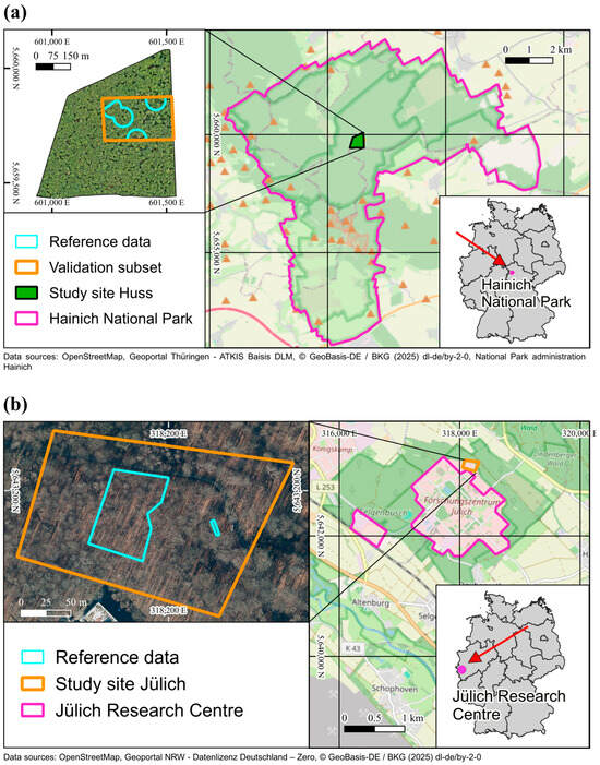
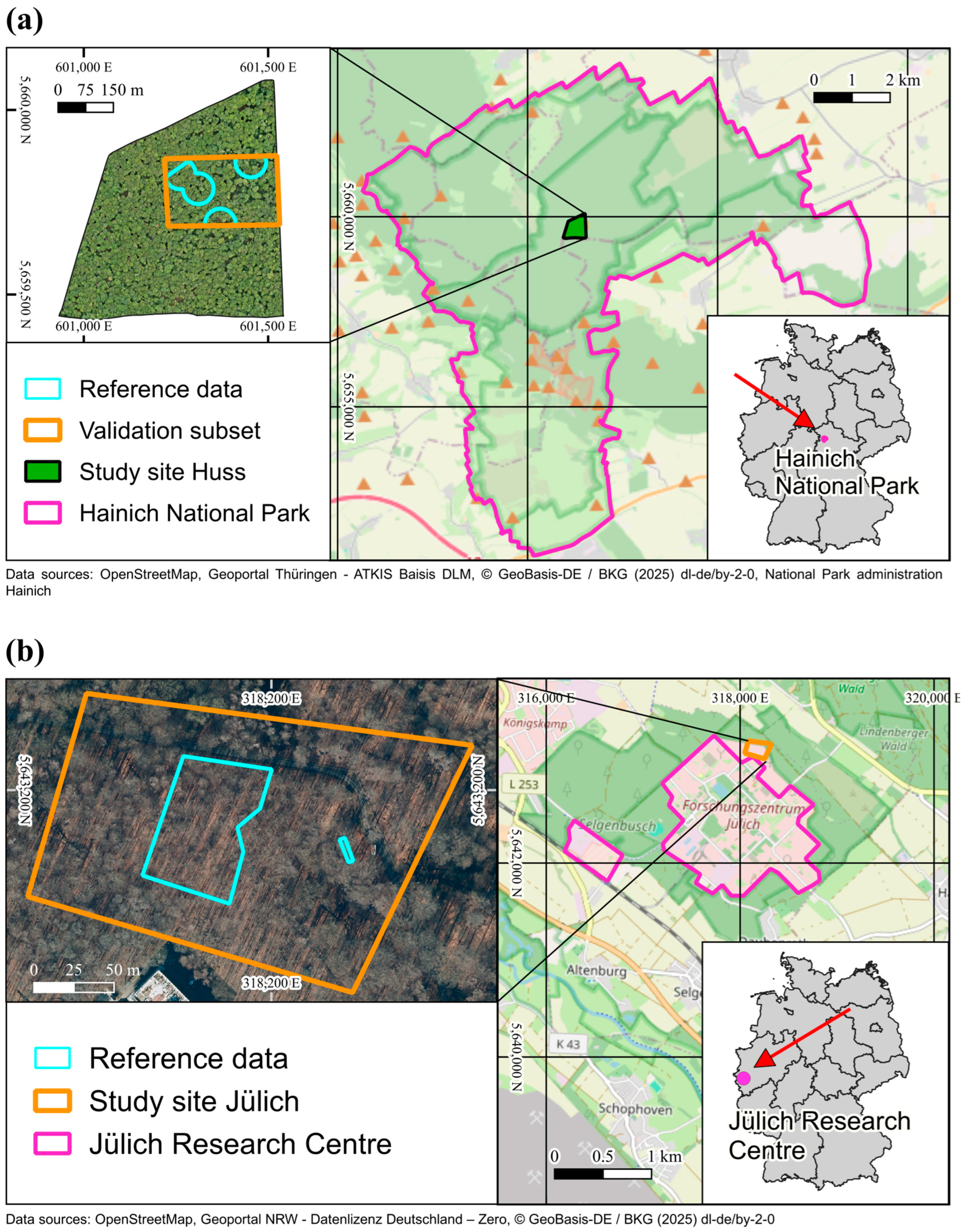
The individual tree detection on SfM point clouds was performed on the so called “Huss site” in the Hainich National Park in Thuringia, Germany (Figure 1a). The study site covers an area of 28.2 ha deciduous forest containing mostly beech (65%), ash (25%) and maple (7%) trees [23]. The tree cover density ranges from 92% to 100% with a mean of 99% [24]. The site is located at an altitude of approximately 400–460 m [25]. For further information about the site, see Dietenberger et al. [11] and Knohl et al. [23]. For this area, no UAV-LiDAR point cloud was available.

Figure 1. Overview of both study areas presenting the areas of reference data and the validation subsets inside. All maps in this paper use an ETRS89/UTM zone 32N projection (Basemaps: OpenStreetMap, https://www.openstreetmap.org/copyright (accessed on 15 May 2026); BKG (2026) dl-de/by-2-0, https://sgx.geodatenzentrum.de/web_public/gdz/datenquellen/datenquellen_vg_nuts.pdf (accessed on 9 October 2025)). (a) The study site in the Hainich National Park, Germany [25]. (b) The study site in Jülich, Germany [26].

2.1.2. Jülich

The second study site is located next to the Research Center in Jülich, Germany (Figure 1b). It was used for the application of the ITSD using UAV-LiDAR data. The study site extends over an area of roughly 3.4 ha on relatively smooth terrain, featuring a temperate deciduous closed-canopy forest with mainly beech and birch trees, with a tree density of approximately 268 trees ha⁻¹. The similar species composition and forest density to those of the Huss site (see Table 1) made this a suitable area for comparison. For further information, see Neuville et al. [6]. For this area, no optical point cloud is available.

Table 1. Summary of the structural characteristics of the reference trees of the Huss and Jülich site. General stand statistics of the Huss site are reported for all mapped trees, whereas DBH and leaning-tree metrics are reported for overstory trees only (std = standard deviation). For the Jülich site, no information about exact tree species or leaning trees was available.

Group	Metric	Value
All trees Huss site	Total number	413
	Tree density (trees/ha)	287.8
	Tree species	Fagus sylvatica (approx. 77%), Fraxinus excelsior, Carpinus betulus, Acer platanoides/pseudoplatanus, Ulmus glabra
Overstory only Huss site	Number	202 (48.9%)
	Tree density (tres/ha)	140.8
	DBH mean ± std (cm)	49.85 ± 24.19
	DBH range (cm)	9.87–121.91
	Leaning trees	11 (5.5%)
Overstory Jülich site	Total number	110
	Tree density (trees/ha)	268.0
	Tree species	Fagus sylvatica (approx. 95%), Betula sp. (approx. 5%)
	DBH mean ± std (cm)	39.05 ± 14.09
	DBH range (cm)	11.0–102.0

2.2. Data

Five datasets were used to perform the ITSD, consisting of four SfM point clouds of the consecutive years from 2022 to 2025 depicting the Hainich National Park and one LiDAR point cloud of the Jülich Forest acquired in 2020 for performance comparison.

2.2.1. Structure-from-Motion Point Clouds

All point clouds were obtained in leaf-off conditions in March in order to enable scanning the whole tree structure and acquiring more accurate images of the stems. The flux tower in Hainich National Park was selected as the take-off and landing site. The first point cloud was recorded on 29 March 2022 using the Da-Jiang Innovations Science and Technology Co., Ltd., Shenzhen, China (DJI) Phantom 4 real-time kinematic (RTK); all following acquisitions were made using the DJI Mavic 3 Enterprise. Overlapping images were recorded by these UAVs equipped with a RTK receiver and an RGB camera. The flight missions were pre-programmed prior to data acquisition and conducted at a flight altitude of 100–110 m above the tower platform, a flight speed of 5–8 m s⁻¹, and image overlaps of 85% front overlap and 80% side overlap. Afterwards, the images were processed in Agisoft Metashape version 2.1.3 to generate a SfM point cloud. The high quality setting was chosen for the SfM point cloud generation, as the study by Tinkham and Woolsey [27] showed that the difference between high and ultra-high quality in Agisoft Metashape hardly has any impact on tree detection results.

Further details on the data acquisition can be seen in Table 2.

Table 2. Overview of the SfM datasets.

Year	Date	Drone	Conducted Flights	Density [pts/m2]
2022	29 March	DJI Phantom 4 RTK	1 × nadir; 2 × 70° oblique	385
2023	21 March	DJI Mavic 3 Enterprise	1 × nadir; 3 × 65° oblique	289
2024	12 March	DJI Mavic 3 Enterprise	1 × nadir; 4 × 65° oblique	305
2025	27 March	DJI Mavic 3 Enterprise	1 × nadir; 4 × 65° oblique	492

All point clouds were height-normalized and clipped to the Huss site using rapidlasso LAStools version 2.0.3.

2.2.2. UAV Laser Scanning Point Cloud

The LiDAR point cloud is the same dataset that was used by Neuville et al. for the estimation of forest structure. For the acquisition, a YellowScan Surveyor LiDAR sensor (YellowScan, Saint-Clément-De-Rivière, France) mounted on a battery-driven DJI Matrice 600 Pro hexacopter was used. The flights were conducted during the leaf-off seasons in November of 2020, using a scan angle range of $\pm$12 degrees. The flight mission was performed at a flight altitude of 50 m, a flight speed of 3 m s⁻¹ above ground, and with an overlap of 70% between the swaths. The point cloud was height-normalized using the ground classification of 3D point cloud data from the open geodata forum of North Rhine Westfalia [26]. The average point density in the Jülich point cloud lies at 236 points/m².

2.2.3. Reference Data

A dataset of manually recorded trees in the Huss site was used as reference data to validate the tree stem detection. The reference set was recorded in 2023. Therefore, the biggest time gap to the point clouds will be two years for the SfM point cloud of 2025 (SfM25). The area in which the reference trees are located is marked in Figure 1a. In total, the inventory included 202 overstory trees and 211 understory trees. The separation into over- and understory was determined on site by visual assessment. Further information, like the diameter at breast height (DBH), tree species and tree leaning, was also documented and is summarized in Table 1. Trees with a DBH below 7 cm were not considered. The positions of the reference trees were used to evaluate the accuracy of the tree stem detection methods, while DBH was used to analyze performance as a function of tree size.

The VCI measures the evenness of point distribution across the entire height of the forest, resulting in lower values if the trees are relatively small (Section 2.3.1). Therefore, understory trees were excluded from the validation, and only overstory trees were used to assess the ITSD performance.

For the Jülich site, a reference dataset containing 110 trees was used. The trees were recorded in September 2020 using the Leica TPS1200 (Leica Camera AG, Wetzlar, Germany) total station and were georeferenced with ground control points, using a Trimble R10 GNSS receiver (Trimble Inc., Westminster, CO, USA) [6]. The DBH of every tree was measured as well, allowing a more thorough analysis of the performance of the ITSD. An overview of the available information can be seen in Table 1.

2.3. Methodology

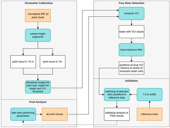
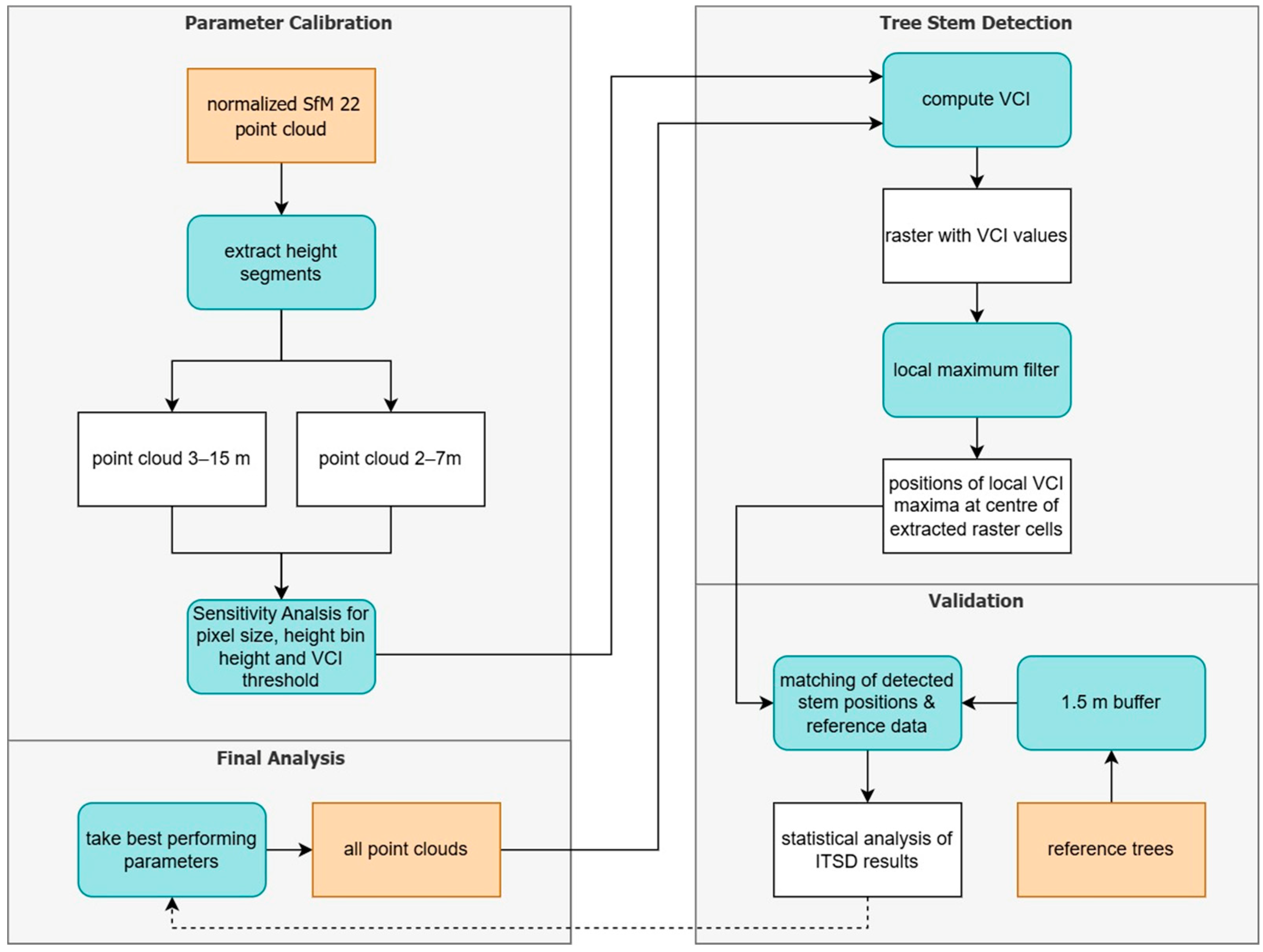
In this study, different aspects of the ITSD were tested. First, using the SfM point cloud from 2022 (SfM22), four parameters were assessed for optimal tree detection with the VCI: the height segment, the spatial resolution, the height bin height (HBH) and the VCI threshold (see Section 2.3.1). SfM22 was chosen because of its relatively high point density in comparison to the point clouds of 2023 (SfM23) and 2024 (SfM24), as well as its acquisition date, which matched well with the reference data (see Table 2 and Section 2.2). Subsequently, the parameter combination that achieved the best tree-detection performance for SfM22 was selected as the standard configuration. This configuration was then applied without further adjustment to all remaining datasets to assess the robustness and transferability of the VCI-based ITSD approach across point clouds acquired in different years. A graphical overview of the workflow can be seen in Figure 2.

Figure 2. Workflow of the individual tree stem detection using the vertical complexity index (VCI) on multiple point clouds. Color coding: orange = input data, blue = processing steps, white = intermediate and final data products.

The ITSD was implemented and executed using PyCharm (v2024.1) and Python 3.12. The analysis was performed on a laptop equipped with an Intel UHD Graphics GPU, an Intel Core i7-10810U processor, and 16 GB of RAM. Processing the tree stem detection workflow for a single dataset required approximately 30 s on this system.

2.3.1. The Vertical Complexity Index

The VCI is based on the Shannon Index, a mathematical index measuring entropy [28] used in the field of ecology for analyzing and quantifying species diversity and species evenness [19,29]. The VCI was adapted by van Ewijk et al. [19] to quantify the distribution of LiDAR point clouds and measure the evenness of the vertical distribution of the points that lie above ground. It is a voxel-based metric for analyzing forest structure and has been used mostly on LiDAR point clouds [30]. The VCI can be computed using the following formula [19]:

$$\mathrm{VCI}={\displaystyle \frac{-{\displaystyle {\sum }_{i=1}^{HB}}\left(p_i\cdot \mathrm{l}\mathrm{n}\left(p_i\right)\right)}{\mathrm{l}\mathrm{n}\left(nHB\right)}}$$

(1)

$nHB$ refers to the number of height bins into which the point cloud is divided, depending on the selected height bin height (HBH). $p_i$ is the proportion of points inside the height bin $i$ relative to the total number of points in the corresponding height column. The x- and y-dimensions of the height column are defined by the chosen raster pixel size. The resulting values can range from 0, meaning all points are concentrated in the same height bin, to 1, meaning the points are evenly spread across the whole height of the point cloud, and all height bins contain the same number of points [19]. In our case, the considered point cloud is the respective UAV-SfM or UAV-LiDAR point cloud.

2.3.2. Testing Parameters and Different Datasets

SfM22 was used for the initial testing of four parameters (height segment, HBH, pixel size, and VCI threshold) to obtain optimal parameter settings.

First, in LAStools, the point cloud was clipped to height ranges of 2–7 m and 3–15 m, respectively, to test different height segments for stem extraction, upon which the VCI was then calculated. The different height segments originate from previous studies that clipped their point clouds for better performance of individual tree detection, corresponding to the stem range between ground and shrubbery and the beginning of the dense canopy. In the case of Hershey et al. [18], it was applied at a mixed species hardwood forest in the United States, also using a voxel-based approach to detect tree stems, using the height segment of 2–7 m. Dietenberger et al. [11] used a clustering algorithm on a 3–15 m point cloud for detecting stem positions in the Huss site, the same study area that is investigated in this study.

Secondly, the VCI was calculated for different spatial resolutions. Many other research studies set a pixel size of 1 m to calculate the VCI [19,31], but in this study, the goal was to test more than one fixed size to be able to adapt to the characteristics of the point cloud and the forest, similar to Brugisser et al. [21]. This enables the evaluation of the influence of the pixel size on the number of detected tree stems. VCI pixel resolutions of 1 m, 0.75 m, 0.5 m and 0.25 m were tested on SfM22, as any bigger pixel size would contradict the goal of detecting single tree stems.

Third, the tree stem detection was applied on SfM22 with an HBH of 1 m, as proposed by van Ewijk et al. [19] and Bruggisser et al. [21]; 0.75 m; 0.5 m like Pearse et al. used [32]; and 0.25 m. In this way, the variation in vertical spatial resolution for computing the VCI would show if there were any differences in the performance of the tree stem detection.

Lastly, three different VCI thresholds were implemented to filter the VCI raster and prevent the detection of local maxima in areas with low VCIs. The three applied thresholds were 0.4, 0.5 and 0.6. The best-performing set of parameters was then applied to all other point clouds.

2.3.3. Conducting the Individual Tree Stem Detection

To detect individual tree stems, the output raster with all VCI values of the Huss site was processed in Python for each point cloud. For this, all VCI values above the VCI threshold were extracted. Afterwards, a local maximum filter was applied, using a neighborhood size of 5 to obtain single pixel locations. The remaining raster cells were transformed into points at the center of the cells and then verified using the reference data.

2.3.4. Accuracy Assessment

The detected stem positions were matched with their closest reference stem up to a maximum distance of 1.5 m. All detected stems with corresponding reference stems within this distance were considered true positives (TP), and the remaining detected stems were assigned false positives (FP). All reference trees which were not detected were considered false negatives (FNs). The distance of 1.5 m was chosen with regard to the average DBH of 49.85 cm for the reference overstory trees (see Table 1). This distance accounts for the positional variability of the tree stem coordinates, which occurred depending on which side of the stem the location was recorded. Taking the VCI raster resolution into account (either 0.5 or 1 m), a buffer of 1.5 m, corresponding to approximately three pixels at 0.5 m resolution or one and a half pixels at 1 m resolution, seemed appropriate for considering all positional uncertainties for the detected stem locations. This radius threshold was also used in the study of Dietenberger et al. [11].

Statistical metrics were used for an accuracy assessment of the ITSD, enabling comparison across different parameter settings as well as between different datasets. Like in previous studies, the Recall, Precision and F1-Score were calculated for all conducted ITSDs [11,13,33]. They are defined as follows:

$$Recall={\displaystyle \frac{\mathrm{T}\mathrm{P}}{\mathrm{T}\mathrm{P}+\mathrm{F}\mathrm{N}}}$$

$$Precision={\displaystyle \frac{\mathrm{T}\mathrm{P}}{\mathrm{T}\mathrm{P}+\mathrm{F}\mathrm{P}}}$$

$$F1\text{-}Score=2\cdot {\displaystyle \frac{Recall\cdot Precision}{Recall+Precision}}$$

Complementary to the accuracy assessment using the overstory reference trees, we also tested if there were any understory reference trees detected.

3. Results

3.1. Assessment of Detection Performance of SfM22 Under Varying Parameters

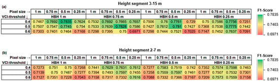
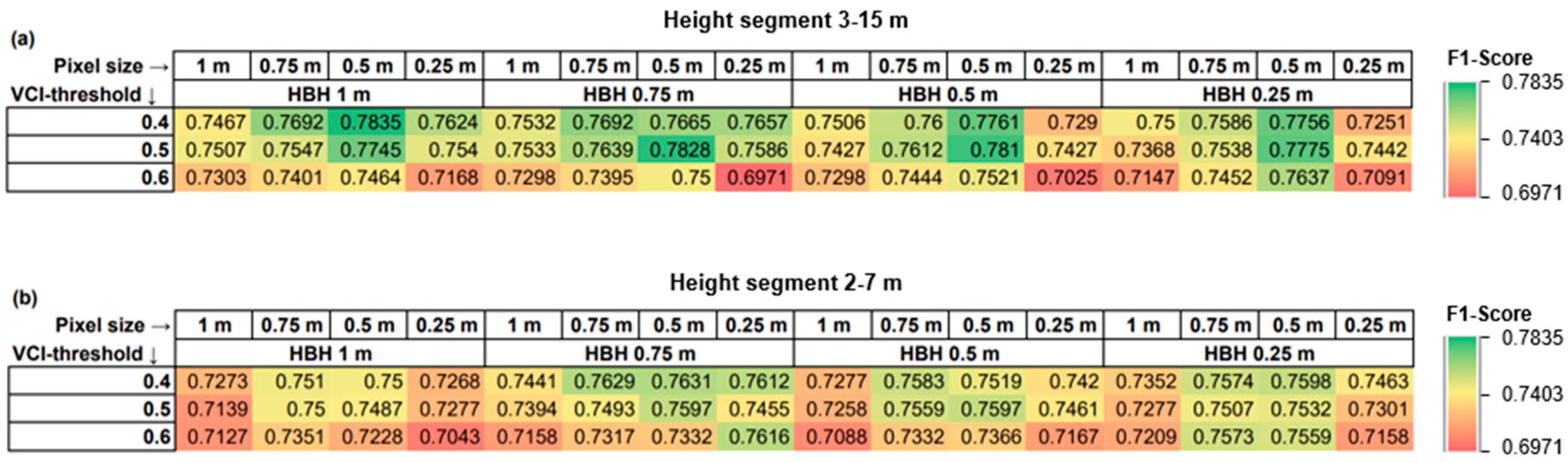
The detection performance of SfM22, considering different point cloud height segments, HBHs, pixel sizes and VCI thresholds, is summarized in Figure 3. The different height segments showed slightly better detection performance for the 3–15 m point cloud in comparison to the 2–7 m point cloud. The pixel size of 0.5 m seemed to perform best in almost any set of parameter combinations. A high VCI threshold of 0.6 decreased the performance of SfM22’s ITSD.

Figure 3. Heatmaps of the sensitivity analysis of SfM22, showing the F1-Scores for each analysis using differing pixel sizes, height bin heights (HBH) and VCI thresholds. The F1-Scores ranged from a minimum of 0.6971 to a maximum of 0.7835. The arrows after a heading indicate the column or row to which they refer. (a) Results for the height segment of 3–15 m. (b) Results for the height segment of 2–7 m.

Varying the HBH resulted in only minor differences in F1-Scores. For the 3–15 m height segment, an HBH of 1 m achieved the highest F1-Score, whereas for the 2–7 m height segment, smaller HBH values showed slightly better performance.

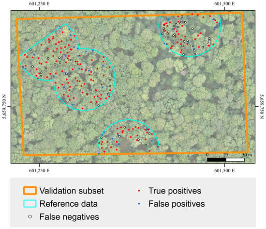
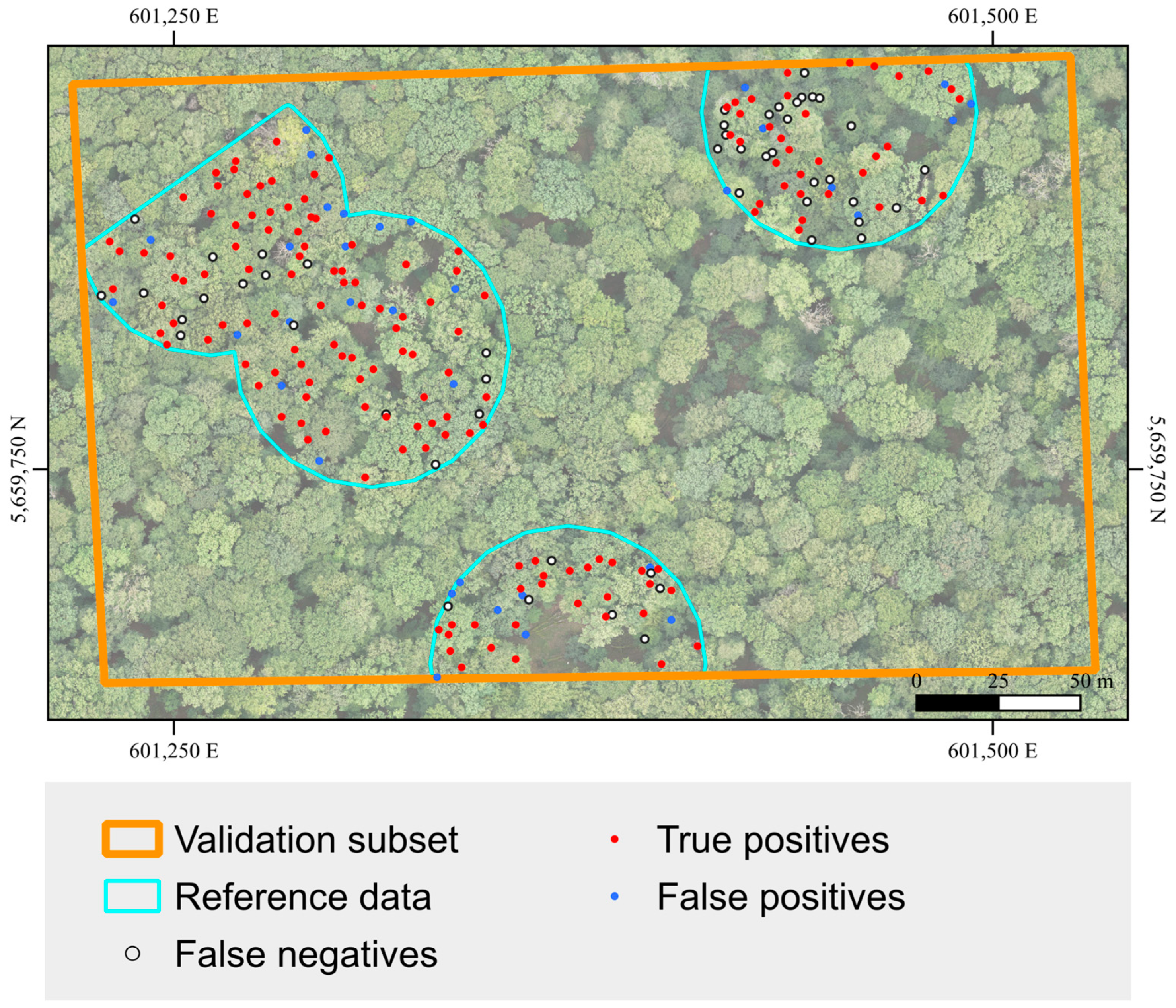
The parameter combination of a 3–15 m height segment, 0.5 m pixel size, 1 m HBH and 0.4 VCI threshold provided the best performance for SfM22. A total of 75.25% of the reference overstory trees were detected, with a Precision of 0.8172 and an F1-Score of 0.7835. A visualization of this result is shown in Figure 4. This parameter set has therefore been chosen to be applied to further datasets.

Figure 4. Results of the individual tree stem detection on SfM22 using a VCI threshold of 0.4, height segment of 3–15 m, pixel size 0.5 m and a 1 m height bin height.

3.2. Comparing ITSD Results of All Datasets

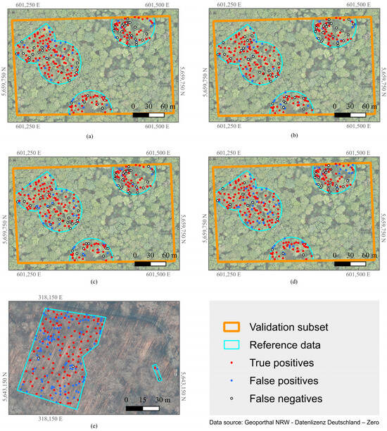
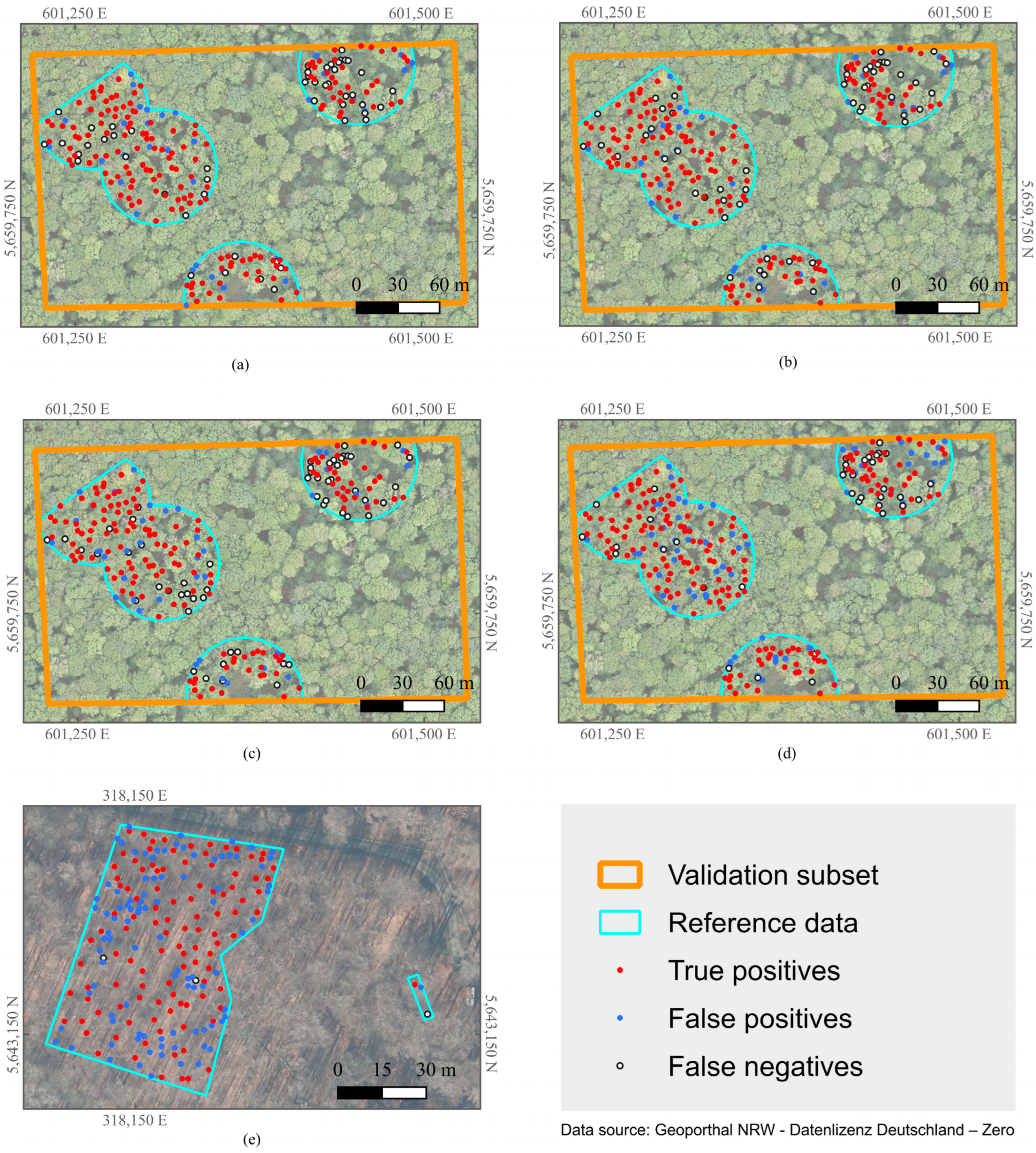
The comparison of the results for all point clouds can be seen in Table 3 and Figure 5. The SfM datasets from 2022 to 2024 all show relatively similar results, while in 2025, a noticeable increase in detected stems occurs. SfM24 finds a minimum of 180 detected stems and 145 TPs, while SfM25 is at a maximum for the SfM ITSD of 226 detected stems with 165 TPs. The highest Precision was measured for SfM22 with a value of 0.82. SfM25 showed the highest Recall of the SfM datasets, where over 80% of the overstory reference trees were detected. Additionally, SfM25 detected the most understory trees when using all reference trees for validation.

Table 3. Results and number of true positives (TPs) of all point clouds using best set of parameters (3–15 m, height bin height 1 m and pixel size 0.5 m with a VCI threshold of 0.4). Bold entries indicate maximum values in that column.

Dataset	Detected Stems Study Site	Detected Stems Validation Area	TPs	TPs over- & Understory (Understory TPs)	Precision	Recall	F1-Score
SfM 22	4093	186	152	173 (+21)	0.8172	0.7525	0.7835
SfM 23	3766	180	147	165 (+18)	0.8167	0.7277	0.7696
SfM 24	3680	185	145	162 (+17)	0.7838	0.7178	0.7494
SfM 25	4624	226	165	203 (+38)	0.7301	0.8168	0.7710
Jülich	2052	202	107	-	0.5297	0.9727	0.6859

Figure 5. Comparison of individual tree stem detection results using height segment 3–15 m, pixel size 0.5 m and height bin height 1 m. (a) SfM22. (b) SfM23. (c) SfM24. (d) SfM25. (e) Jülich UAV-LiDAR point cloud.

However, the largest performance difference is observed when applying the method to the UAV-LiDAR point cloud instead of the SfM datasets. Using the selected optimum parameters (see Section 2.3.2) on the UAV-LiDAR dataset, there were 202 stems detected in the significantly smaller validation area of the Jülich site. A total of 107 of the 110 reference trees were detected, which makes this the highest Recall value of all datasets with 0.97. The Precision, though, only producing a value of 0.53 with 95 FPs, is still in the lower range. To assess whether this represents a general limitation of the VCI approach or a site-specific parameter mismatch, we tested different parameter combinations adapted to the local conditions at the Jülich site. This improved the performance significantly, with the best result obtained at a VCI threshold of 0.8, resulting in an F1-Score of 0.86, with a 0.89 Recall and 0.82 Precision.

3.3. Influence of Forest Conditions on Detection Performance

The statistical results of the SfM datasets were further analyzed, using the SfM22 dataset, since it was the dataset which was used for calibrating all parameters. The time difference between SfM22 and the reference data is only one year; therefore, it can be assumed that the bias regarding possible changes in forest inventory is negligible. The results of the Jülich site were also analyzed in the aspects that its reference data could provide.

3.3.1. Leaning Trees and Detection of Understory Trees

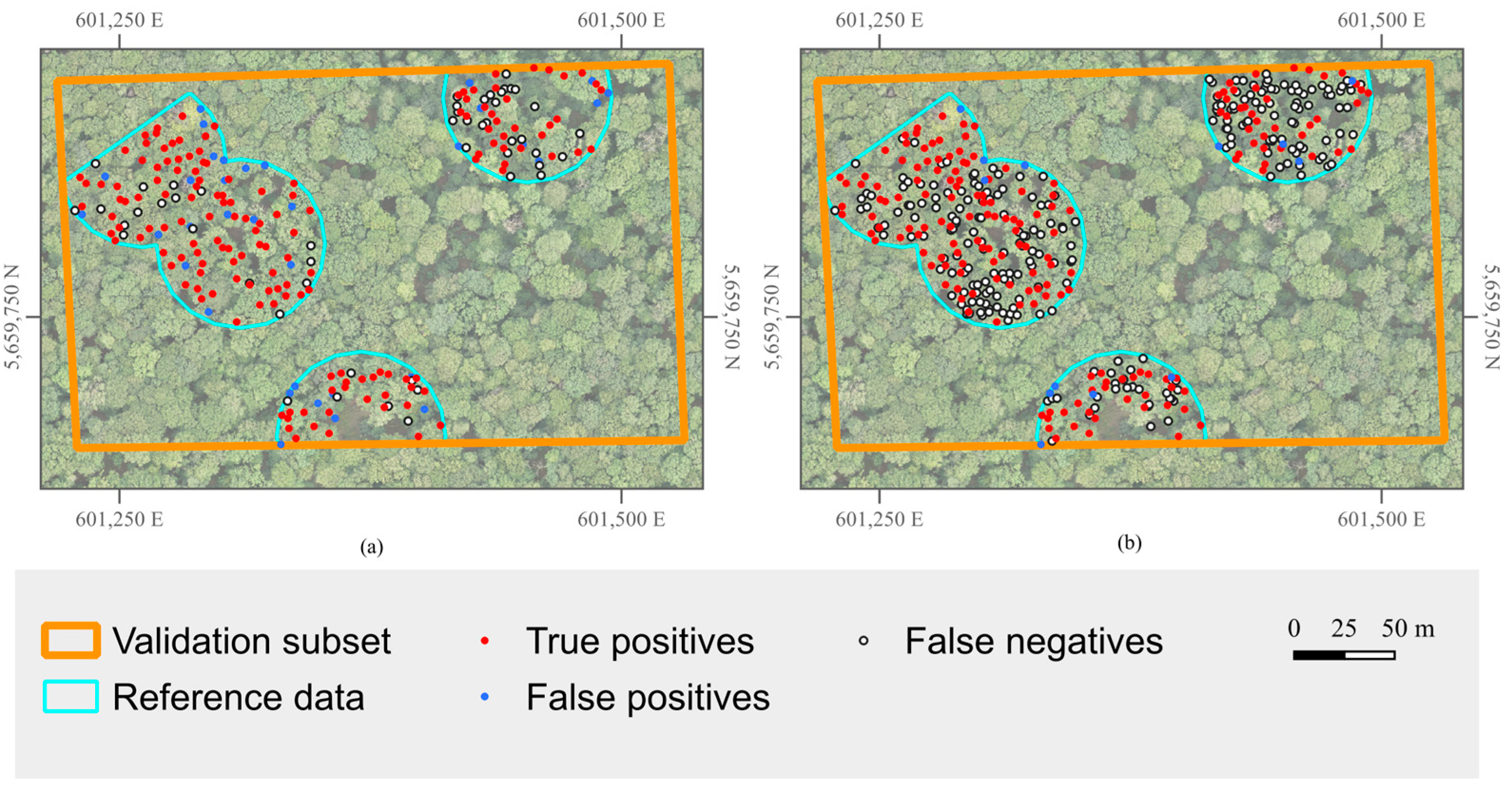
In each of the four acquisition years of the SfM point clouds, four to six stems of the eleven documented leaning trees were detected. The remaining stems were counted as FNs. A comparison of the SfM22 results using overstory reference trees versus using over- and understory trees is shown in Figure 6. The ITSD on SfM22 detected 186 stems in total, of which 152 were TPs when using the overstory reference trees for validation. Of the 34 FPs, 21 could be matched with understory trees, which means that only 13 FPs were detected and over 93% of all detected stems could be matched to reference trees when understory trees were considered. Applying this to all SfM datasets, Precision lies above 87% for each point cloud.

Figure 6. Comparison of SfM22 individual tree stem detection results using VCI threshold 0.4, height segment 3–15 m, pixel size 0.5 m and height bin height 1 m, validating with different reference datasets. (a) Only overstory trees as reference dataset. (b) Over- and understory trees as reference dataset.

However, the majority of understory trees were still not detected, resulting in a Recall of 41.89% for SfM22 considering all (over- and understory) trees.

3.3.2. Forest Density

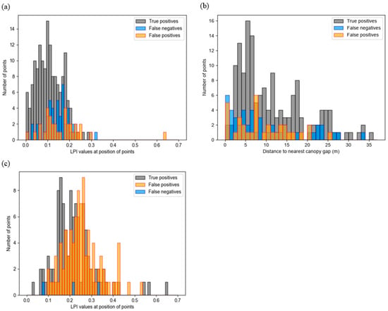
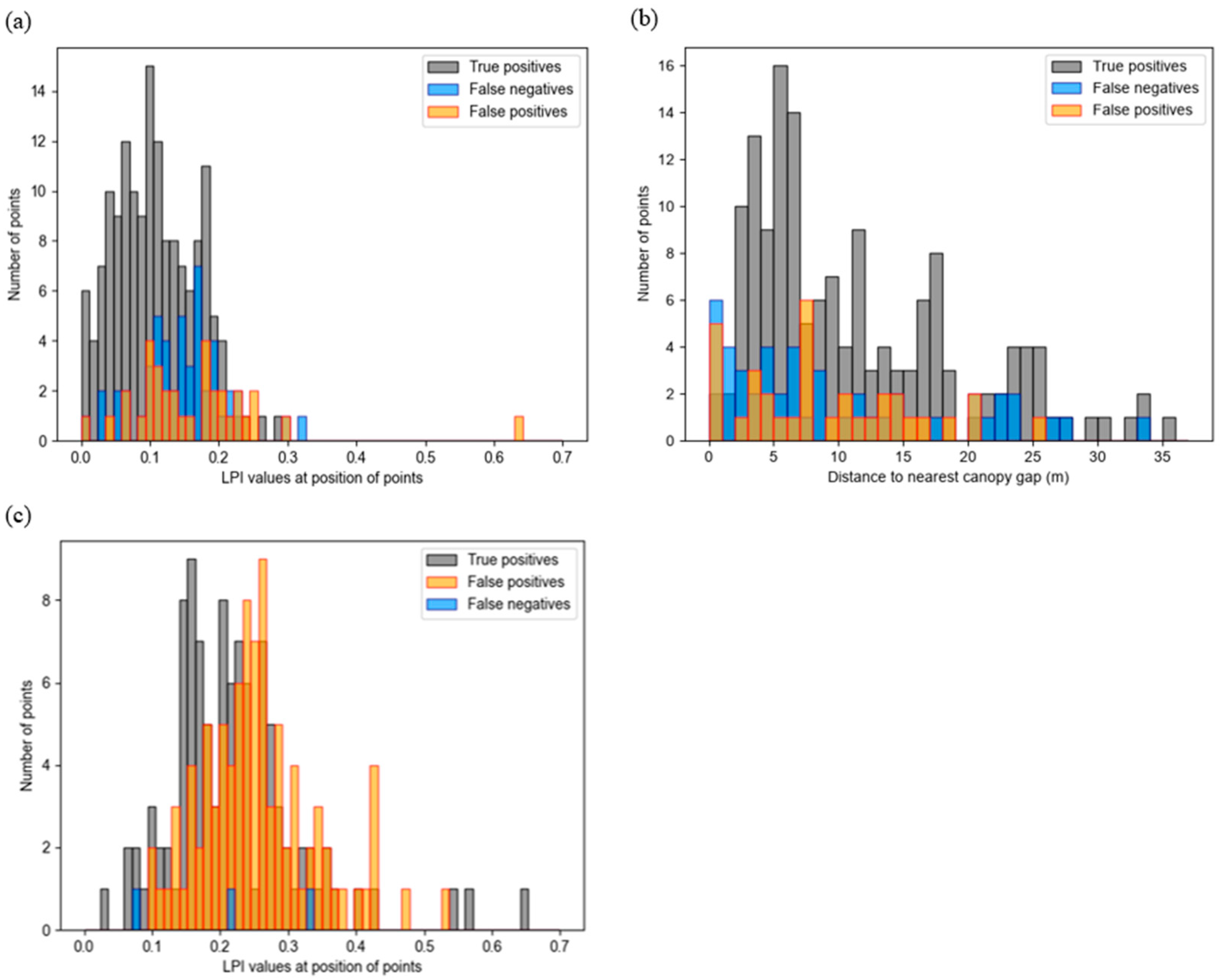
An indicator of vegetation density is the Laser Penetration Index (LPI), which is computed as the ratio of ground points to all points in each raster cell [34]. The FNs and TPs of the SfM22 ITSD were compared by looking at their respective LPI values to determine if the forest density might be a source of error for detecting tree stems. The LPI was computed using the Airborne Laser Scanning point clouds provided by GDI-Th and [25] to ensure an independent forest density metric that does not contain the same possible data gaps as the SfM point cloud.

As can be seen in the histogram in Figure 7a, the LPI values for FNs are slightly higher than the LPI values of the TPs. A Wilcoxon rank-sum test for FNs and TPs, as well as a Kruskal–Wallis test for all three categories, proved the difference to be statistically significant (alpha = 0.01). This suggests that reference trees which were detected with the algorithm lie in slightly denser forest parts. Yet, the differences are rather marginal and could be specific to this point cloud.

Figure 7. Histogram showing density metrics of the false negatives, false positives and true positives from the individual tree stem detection, using (a) the Laser Penetration Index (LPI) values for SfM22; (b) the distance to the nearest canopy gap for SfM22; (c) the LPI values for Jülich UAV-LiDAR data.

As additional independent metrics, the distance of FNs, TPs and FPs to the nearest canopy gap was calculated for the Huss site. All visible gaps in the overstory canopy were manually recorded and the distances of the FNs, TPs and FPs of SfM22 were computed. The results can be seen in Figure 7b. The differences in TPs, FNs and FPs did not prove to be statistically significant (alpha = 0.05).

For the Jülich dataset, the LPI was calculated using the Airborne Laser Scanning point cloud provided by the federal geodata portal, which was used for normalizing the point cloud [26]. An analysis of canopy gaps was not done for this study site, as the canopy density is very evenly distributed across the validation area and there were no clear canopy gaps to assess.

As can be seen in Figure 7b, the difference in LPI values between TPs and FPs is similar to SfM22. The FPs lie in slightly less dense forest parts in comparison to the TPs. There are only three FNs, which are spread over different forest densities. The difference in LPI between FPs and TPs was statistically significant at an alpha value of 0.01.

3.3.3. DBH

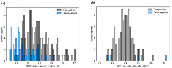
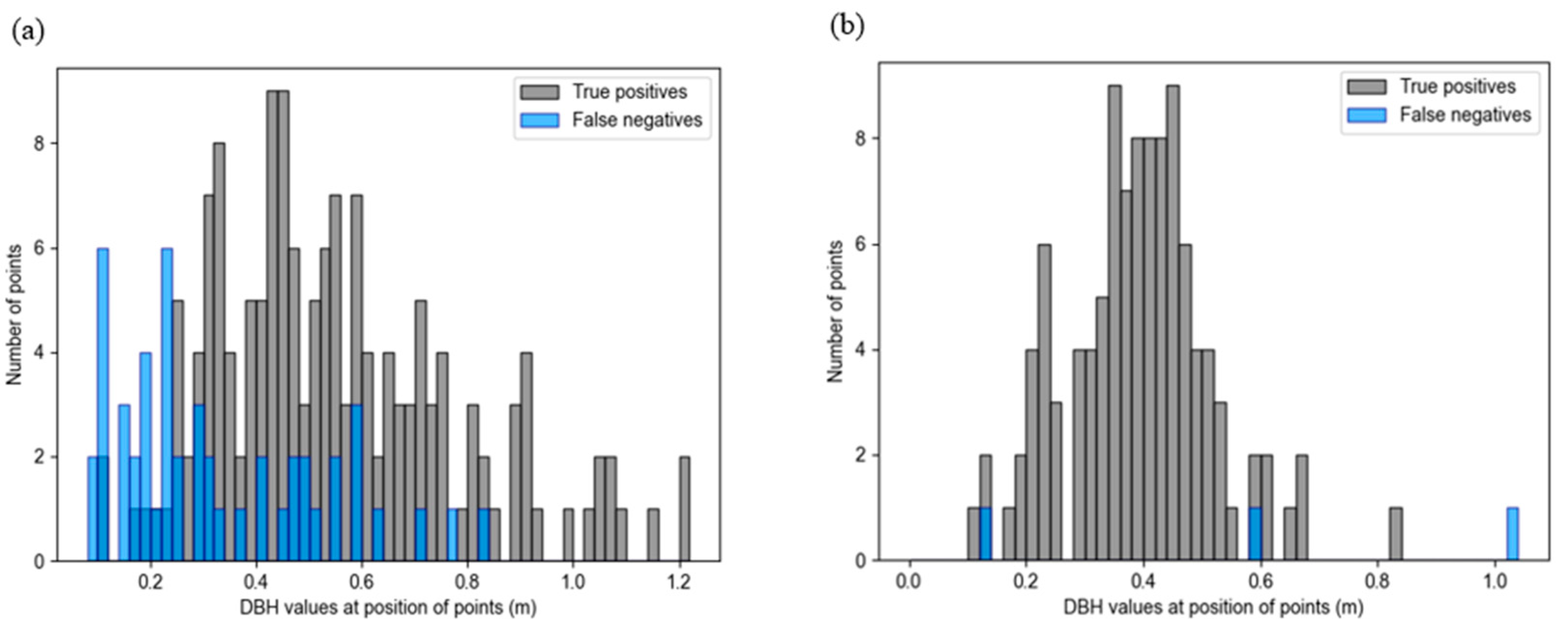
Looking at the DBH values of reference trees that were not detected in SfM22, it becomes clear that the mean DBH of FNs is lower than that of the TPs. The histogram in Figure 8a shows that trees with a DBH of less than 0.25 m were particularly hard to detect. Four trees with DBH values greater than 0.6 m were not detected, and two of them were marked as having a leaning stem. A Wilcoxon rank-sum test showed that the difference in DBH between FNs and TPs is statistically significant (alpha = 0.01).

Figure 8. Histogram showing the diameter at breast height (DBH) values of the false negatives and true positives from the individual tree stem detection using (a) SfM22 and (b) Jülich UAV-LiDAR data.

In the Jülich forest site, only three trees were not detected; all of them showed drastically different DBH values, as can be seen in Figure 8b, ranging from 13 cm to over 1 m.

4. Discussion

Voxel-based approaches for tree stem detection are strongly dependent on their spatial resolution, which has to be considered when analyzing the results [18]. In this study, all results should therefore be interpreted in the context of the chosen voxel size (pixel size and HBH) for the computation of the VCI. Tree stem positions were appointed at the center of each pixel, which can lead to small horizontal offsets. Additionally, as Hershey et al. noted in their study, the location of a tree stem is not a definitive point, as stems lean and fork, and therefore spatial accuracy must be viewed in a nuanced way [18].

It also has to be noted that there was a maximum time difference of three years between the SfM point clouds and only one reference dataset for the Huss site. Therefore, differences in forest composition may have affected the accuracy assessment. Nonetheless, these differences are likely confined primarily to the understory, given the short time span relative to tree growth.

4.1. Parameter Assessment

When comparing the two height segments 2–7 m and 3–15 m, the latter performed better on SfM22. This could mean that the additional stem points that are contained in the 3–15 m segment are beneficial for a more robust VCI differentiation between the stem and other points. In addition, the higher minimum helps in excluding more shrubs and understory vegetation points, which could disturb the ITSD. Overstory trees may have more stem points at higher heights like in the segment 3–15 m, because the optical drone sensor has a better viewing angle on the stems if no other branches or understory stems next to the overstory stem are obscuring them. This is probably the reason why the 3–15 m segment height, which was also used by Dietenberger et al. in their stem detection algorithm, performed better for this study area [11].

When testing the pixel size, a resolution of 1 m produced lower tree detection rates than the resolutions of 0.75 m and especially 0.5 m. This was expected, as the point densities of the SfM datasets are more than sufficient for a voxel size of 0.5 m edge length. With smaller pixel sizes, the tree stems can also be better distinguished from each other, while with larger pixel sizes, the possibility of more than one stem per pixel increases, leading to more FNs.

The resolution of the HBH products did not affect the ITSD’s performance as much as the pixel size. Yet, a separation into fewer but larger vertical height bins, using 1 m, might have produced the best results because SfM is not able to penetrate existing vegetation and therefore, the VCI is more robust when using a bigger resolution in the vertical dimension.

4.2. Comparison of SfM Dataset and Previous Studies

The ITSD approach using VCI with SfM point clouds showed that results align well with previous studies that used different tree detection methods on the SfM and LiDAR datasets [11,27,35,36]. In Tinkham and Woolsey’s analysis of different processing parameters for SfM data and their influence on individual tree detection, the average F1-Score of high density point clouds processed in Agisoft Metashape ranged from approximately 0.5 to 0.7 [27]. Hershey et al. achieved an overall detection rate of 67.73% by using their voxel-based approach to stem detection, which is slightly lower than the overall detection rate of 75.37% for the four SfM datasets in this study [18]. Mohan et al. recorded an average Recall of 75% for SfM data [35]. It must be noted that there is no standard for matching reference trees with detected trees and lots of studies use a wider radius than the 1.5 m used in this study [18,27,36,37]. Dietenberger et al., who also used the threshold of 1.5 m in their study of the Huss site, observed an F1-Score of 0.8 when using only overstory reference trees. However, even though they did not specify a computational time, the clustering algorithm Dietenberger et al. used can be assumed to be more time-consuming than the method proposed in this study, which only required about 30 s of computation time on a standard laptop (see Section 2.3) [11].

The ITSD results of SfM25 stood out compared to the other SfM point clouds, as there were significantly more stems detected, resulting in a higher Recall. In terms of point density, SfM25 exceeds all other SfM datasets by more than 100 points/m². The flight number and angles of the UAV were the same in 2025 as they were in 2024, yet SfM24 is considerably less dense. The only difference in acquisition that could be determined was the weather condition, which in 2025 was a clear sky, while all other UAV flights were conducted when the sky was overcast. This could mean that for the generation of an SfM leaf-off point cloud, sunny weather and clear skies might lead to better representation of tree stems and help in detecting tree stem positions. Similar tendencies were observed in other studies [38,39]. However, this remains a hypothesis based on a single observation and requires further quantitative investigation. Apart from SfM25, all SfM ITSDs were fairly similar and showed robust results of the method.

4.3. UAV-LiDAR Point Cloud

Laser scanning technology is generally effective at penetrating the canopy and detecting structural elements like tree stems and often performs slightly better at detecting trees in comparison to SfM datasets [35,40]. However, when applying the selected parameter set to the Jülich UAV-LiDAR dataset, the overall performance did not reach the same accuracy as the SfM datasets. Although it achieved the highest overall Recall, detecting more than 97% of trees, this achievement was offset by a high number of false positives.

This is likely related to the fact that the ITSD parameters were optimized using an SfM dataset and may therefore not be optimal for application to a LiDAR point cloud. This is why some other combinations were tested on the UAV–LiDAR point cloud, for example a higher VCI threshold to reduce the number of FPs, resulting in a performance that even outperforms the SfM datasets. The higher VCI threshold mitigated smaller local VCI maxima, which produced a lot of FPs in the previous ITSD. These findings suggest that for the application of this ITSD method, an additional calibration of the VCI threshold may be necessary to enhance its performance.

The adjusted ITSD performed well in accordance with other studies using different tree detection methods on UAV–LiDAR point clouds, especially considering the reduced processing power of the method compared to other methods which do not use the VCI [35,41].

4.4. Detection of Leaning and Understory Trees

Several of the leaning stems were not detected, which could be explained by their division into multiple columns during VCI computation. This leads to a less uniform vertical distribution of points and, consequently, a lower VCI, preventing their detection by the local maxima filter.

The number of undetected understory tree stems can be explained by lower tree height and lower DBH values for understory trees, which both have been proven to cause lower tree detection rates [18]. In addition, the computation of high VCI values relies on even distribution across the entire height segment, which in this case would adversely affect any tree smaller than 15 m. The selection of the height segment will therefore likely influence the performance of the ITSD regarding the height of the trees that are detected.

4.5. Influence of Forest Density and DBH on the Performance of the Individual Tree Stem Detection

In previous studies, errors in detecting trees could sometimes be linked to higher forest density [9,42]. SfM data relying on the visibility range of the camera can fail to capture objects near the ground in areas with dense vegetation [12]. The higher LPI values of TPs in comparison to FNs at the Huss site are therefore surprising, as other studies often showed greater difficulties in detecting stems in denser parts of the forest [9,12,42].

However, the difference in distances to the nearest canopy gap between TPs and FNs did not prove to be significant. Therefore, it can be assumed that the reason for undetected tree stems at the Huss site does not originate from a difference in canopy cover.

The high number of FPs at the Jülich study site was also located in less dense areas of the forest. This suggests that regardless of the acquisition technique, there were no major issues in detecting tree stems in denser parts of the forest. Given that the difference in LPI values between TPs and FPs is relatively small, the higher LPI values for FPs are likely not meaningful.

It has to be noted that the LPI can be influenced by terrain conditions and acquisition parameters [43]. However, the terrain across the Huss site is relatively flat, and the ALS data used for the analysis were acquired using the same flight system and acquisition settings. Therefore, we do not expect within-dataset distortions caused by these factors. One possible explanation could be that the LPI produces a similar result to the VCI rasters at 1 m resolution, as it also calculates a ratio of points in the point cloud. The pixels with the lowest LPI values, indicating denser forest, would therefore be at the location of tree stems. This would then show that FPs, which are further from the positions of reference tree stems, lie in less dense areas. This may also indicate that the forest structure observed in the Airborne Laser Scanning point clouds overlaps significantly with that of the SfM datasets, further proving that the scanning of tree stems using optical data during leaf-off season was very successful.

With regard to DBH, more tangible statements can be made about the detection of tree stems. Two of the SfM22 FNs with a DBH above 0.6 m could be traced back to a leaning stem, explaining the reason for their omission. The other two trees both showed relatively low VCI values at their positions, which may be due to the fact that SfM cannot penetrate the forest canopy, and bigger trees with more branches could obscure the view of the tree stem.

The results of SfM22 indicate that the DBH significantly affects the ITSD performance, with better detection rates at the higher DBH values. Approximately 81% of overstory trees with a DBH $\ge$ 0.2 m and 91% of overstory trees with DBH values $\ge$ 0.6 m were detected at the Huss site. This link between detection rates and DBH was also found in the study of Hershey et al. [18].

At the Jülich site, only three tree stems were not detected, all of them having drastically different DBH values. As there was no data on leaning of trees for this study site, it is not clear if that was the reason for some of the FNs. When using the adjusted parameters with a VCI threshold of 0.8 for the Jülich point cloud, 60% of the FNs showed a DBH under 0.5 m, with only two undetected trees having a DBH $>$ 0.6 m. This suggests that for the UAV-LiDAR point cloud, there may be the same connection between low DBH and lower detection of tree stems as for the SfM datasets.

4.6. Future Challenges in the Application of the Method

So far, this newly developed tree detection method using VCI has only been tested on two study sites which both contain temperate deciduous forests. In order to make more general statements about the method’s robustness, it needs to be tested on more diverse forest types, possibly in different climate zones.

The conducted study is based on leaf-off data, which can only be acquired in deciduous forests during winter months or outside the growing season, as long as the drone flies above the canopy. The applicability of the method to coniferous stands or deciduous forests during the growing season (leaf-on conditions) was not assessed in this study, but occlusion might be an additional challenge in these cases, unless other data acquisition methods that can scan underneath the canopy, like terrestrial laser scanning, are used. For coniferous and leaf-on deciduous trees, VCI values may show higher values at the edge of the crown compared to the stem position, which could potentially help delineate individual tree crowns. However, this remains speculative and further investigation is needed to evaluate the method’s applicability to coniferous and deciduous leaf-on stands.

Even though some leaning stems were detected, the VCI depends on the relative vertical shapes of the tree stems. This complicates the detection of leaning trees or forests with structures that are not dominated by vertical tree elements.

5. Conclusions

Individual tree detection is an important component of forest inventory and can support forest management, restoration, and conservation. This study introduced a voxel-based ITSD method for SfM point clouds based on the VCI. While the VCI has previously been applied primarily to LiDAR data, this study demonstrated its use for optical UAV-SfM point clouds as a comparatively simple and time-efficient alternative to established ITSD approaches.

The method was evaluated using four UAV-SfM point clouds acquired between 2022 and 2025 in the Hainich National Park, Germany, and one UAV-LiDAR point cloud from Jülich, Germany. Parameter calibration on SfM22 identified a VCI threshold of 0.4, a pixel size of 0.5 m, a height bin height of 1 m, and a height segment of 3–15 m as the most effective configuration. Across the SfM datasets, F1-Scores of up to 0.78 were achieved, with Recall and Precision values ranging from 0.73 to 0.82. Precision exceeded 0.93 when documented understory trees were included in the validation.

The method showed limitations in detecting small trees (DBH < 25 cm), understory trees, and leaning stems. These limitations are associated with reduced stem visibility in optical point clouds and with the VCI’s dependence on vertically structured stem representations. Acquisition conditions also appeared to influence performance, as the SfM dataset acquired under more favorable weather conditions detected substantially more stems; however, this observation requires further investigation.

When applied to UAV-LiDAR data using the SfM-derived parameter set, the method achieved an F1-Score of 0.69. After adjusting the VCI threshold, performance increased to an F1-Score of 0.86, exceeding the results obtained for the SfM datasets. This demonstrates that the VCI-based approach can be transferred across point-cloud types and study sites, although parameter adjustment may be necessary to account for differences in acquisition technique and point density.

Overall, the proposed VCI-based ITSD method achieved performance comparable to established clustering- and canopy-height-model-based approaches while offering a more straightforward and less time-intensive workflow. Its successful application to RGB-derived SfM point clouds provides a potentially lower-cost alternative to LiDAR-based tree detection for forest inventory. Future work should assess the method in additional forest types, including coniferous stands and leaf-on deciduous forests, and further evaluate the effects of acquisition conditions and point-cloud characteristics.

References

- Jeronimo, S.M.A.; van Kane, R.; Churchill, D.J.; McGaughey, R.J.; Franklin, J.F. Applying LiDAR Individual Tree Detection to Management of Structurally Diverse Forest Landscapes. J. For. 2018, 116, 336–346. [Google Scholar] [CrossRef] [Scilit]
- Goodbody, T.R.H.; Coops, N.C.; White, J.C. Digital Aerial Photogrammetry for Updating Area-Based Forest Inventories: A Review of Opportunities, Challenges, and Future Directions. Curr. For. Rep. 2019, 5, 55–75. [Google Scholar] [CrossRef] [Scilit]
- Kuang, W.; Ho, H.W.; Zhou, Y.; Suandi, S.A.; Ismail, F. A comprehensive review on tree detection methods using point cloud and aerial imagery from unmanned aerial vehicles. Comput. Electron. Agric. 2024, 227, 109476. [Google Scholar] [CrossRef] [Scilit]
- Carrivick, J.L.; Smith, M.W.; Quincey, D.J. Structure from Motion in the Geosciences; Wiley Blackwell: Chichester, UK, 2016. [Google Scholar]
- Iglhaut, J.; Cabo, C.; Puliti, S.; Piermattei, L.; O’Connor, J.; Rosette, J. Structure from Motion Photogrammetry in Forestry: A Review. Curr. For. Rep. 2019, 5, 155–168. [Google Scholar] [CrossRef] [Scilit]
- Neuville, R.; Bates, J.S.; Jonard, F. Estimating Forest Structure from UAV-Mounted LiDAR Point Cloud Using Machine Learning. Remote Sens. 2021, 13, 352. [Google Scholar] [CrossRef] [Scilit]
- Xiong, J.; Fang, Y.; Jin, B.; Zhao, Z. Automated DTM Generation in Urban Areas with Airborne LiDAR Data. In Proceedings of the 2012 4th International Conference on Intelligent Human-Machine Systems and Cybernetics (IHMSC 2012), Nanchang, China, 26–27 August 2012; IEEE: Piscataway, NJ, USA, 2012; pp. 181–184. [Google Scholar]
- Ozcan, A.H.; Unsalan, C. LiDAR Data Filtering and DTM Generation Using Empirical Mode Decomposition. IEEE J. Sel. Top. Appl. Earth Obs. Remote Sens. 2017, 10, 360–371. [Google Scholar] [CrossRef] [Scilit]
- Mohan, M.; Silva, C.; Klauberg, C.; Jat, P.; Catts, G.; Cardil, A.; Hudak, A.; Dia, M. Individual Tree Detection from Unmanned Aerial Vehicle (UAV) Derived Canopy Height Model in an Open Canopy Mixed Conifer Forest. Forests 2017, 8, 340. [Google Scholar] [CrossRef] [Scilit]
- Guerra-Hernández, J.; Cosenza, D.N.; Rodriguez, L.C.E.; Silva, M.; Tomé, M.; Díaz-Varela, R.A.; González-Ferreiro, E. Comparison of ALS- and UAV(SfM)-derived high-density point clouds for individual tree detection in Eucalyptus plantations. Int. J. Remote Sens. 2018, 39, 5211–5235. [Google Scholar] [CrossRef] [Scilit]
- Dietenberger, S.; Mueller, M.M.; Bachmann, F.; Nestler, M.; Ziemer, J.; Metz, F.; Heidenreich, M.G.; Koebsch, F.; Hese, S.; Dubois, C.; et al. Tree Stem Detection and Crown Delineation in a Structurally Diverse Deciduous Forest Combining Leaf-On and Leaf-Off UAV-SfM Data. Remote Sens. 2023, 15, 4366. [Google Scholar] [CrossRef] [Scilit]
- Wallace, L.; Lucieer, A.; Watson, C.S. Evaluating Tree Detection and Segmentation Routines on Very High Resolution UAV LiDAR Data. IEEE Trans. Geosci. Remote Sens. 2014, 52, 7619–7628. [Google Scholar] [CrossRef] [Scilit]
- Sparks, A.M.; Corrao, M.V.; Smith, A.M.S. Cross-Comparison of Individual Tree Detection Methods Using Low and High Pulse Density Airborne Laser Scanning Data. Remote Sens. 2022, 14, 3480. [Google Scholar] [CrossRef] [Scilit]
- Chen, Q.; Gao, T.; Zhu, J.; Wu, F.; Li, X.; Lu, D.; Yu, F. Individual Tree Segmentation and Tree Height Estimation Using Leaf-Off and Leaf-On UAV-LiDAR Data in Dense Deciduous Forests. Remote Sens. 2022, 14, 2787. [Google Scholar] [CrossRef] [Scilit]
- Vaughn, N.R.; Moskal, L.M.; Turnblom, E.C. Tree Species Detection Accuracies Using Discrete Point Lidar and Airborne Waveform Lidar. Remote Sens. 2012, 4, 377–403. [Google Scholar] [CrossRef] [Scilit]
- Wu, B.; Yu, B.; Yue, W.; Shu, S.; Tan, W.; Hu, C.; Huang, Y.; Wu, J.; Liu, H. A Voxel-Based Method for Automated Identification and Morphological Parameters Estimation of Individual Street Trees from Mobile Laser Scanning Data. Remote Sens. 2013, 5, 584–611. [Google Scholar] [CrossRef] [Scilit]
- Brolly, G.; Király, G.; Lehtomäki, M.; Liang, X. Voxel-Based Automatic Tree Detection and Parameter Retrieval from Terrestrial Laser Scans for Plot-Wise Forest Inventory. Remote Sens. 2021, 13, 542. [Google Scholar] [CrossRef] [Scilit]
- Hershey, J.L.; McDill, M.E.; Miller, D.A.; Holderman, B.; Michael, J.H. A Voxel-Based Individual Tree Stem Detection Method Using Airborne LiDAR in Mature Northeastern U.S. Forests. Remote Sens. 2022, 14, 806. [Google Scholar] [CrossRef] [Scilit]
- van Ewijk, K.Y.; Treitz, P.M.; Scott, N.A. Characterizing Forest Succession in Central Ontario using Lidar-derived Indices. Photogramm. Eng. Remote Sens. 2011, 77, 261–269. [Google Scholar] [CrossRef] [Scilit]
- Gril, E.; Laslier, M.; Gallet-Moron, E.; Durrieu, S.; Spicher, F.; Le Roux, V.; Brasseur, B.; Haesen, S.; van Meerbeek, K.; Decocq, G.; et al. Using airborne LiDAR to map forest microclimate temperature buffering or amplification. Remote Sens. Environ. 2023, 298, 113820. [Google Scholar] [CrossRef] [Scilit]
- Bruggisser, M.; Hollaus, M.; Kükenbrink, D.; Pfeifer, N. Comparison of Forest Structure Metrics Derived from Uav Lidar and Als Data. ISPRS Ann. Photogramm. Remote Sens. Spat. Inf. Sci. 2019, 4, 325–332. [Google Scholar] [CrossRef] [Scilit]
- LaRue, E.A.; Fahey, R.; Fuson, T.L.; Foster, J.R.; Matthes, J.H.; Krause, K.; Hardiman, B.S. Evaluating the sensitivity of forest structural diversity characterization to LiDAR point density. Ecosphere 2022, 13, e4209. [Google Scholar] [CrossRef] [Scilit]
- Knohl, A.; Schulze, E.-D.; Kolle, O.; Buchmann, N. Large carbon uptake by an unmanaged 250-year-old deciduous forest in Central Germany. Agric. For. Meteorol. 2003, 118, 151–167. [Google Scholar] [CrossRef] [Scilit]
- European Environment Agency. Tree Cover Density 2018–Present (Raster 10 m); European Environment Agency: Copenhagen, Denmark, 2024. [Google Scholar]
- GDI-Th. Geodateninfrastruktur TH—Download Offene Geodaten—Download Höhendaten. Available online: https://geoportal.thueringen.de/gdi-th/download-offene-geodaten/download-hoehendaten (accessed on 20 August 2025).
- IT.NRW. Geobasisdaten. Available online: https://www.opengeodata.nrw.de/produkte/geobasis/ (accessed on 15 April 2026).
- Tinkham, W.T.; Woolsey, G.A. Influence of Structure from Motion Algorithm Parameters on Metrics for Individual Tree Detection Accuracy and Precision. Remote Sens. 2024, 16, 3844. [Google Scholar] [CrossRef] [Scilit]
- Shannon, C.E.; Weaver, W. The Mathematical Theory of Communication; University of Illinois Press: Urbana, IL, USA, 1949. [Google Scholar]
- MacArthur, R.H.; MacArthur, J.W. On Bird Species Diversity. Ecology 1961, 42, 594–598. [Google Scholar] [CrossRef] [Scilit]
- Pearse, G.D.; Watt, M.S.; Dash, J.P.; Stone, C.; Caccamo, G. Comparison of models describing forest inventory attributes using standard and voxel-based lidar predictors across a range of pulse densities. Int. J. Appl. Earth Obs. Geoinf. 2019, 78, 341–351. [Google Scholar] [CrossRef] [Scilit]
- Ross, C.W.; Loudermilk, E.L.; O’Brien, J.J.; Snitker, G. Lidar-derived structural-complexity data across four experimental forests. Data Brief 2024, 57, 110955. [Google Scholar] [CrossRef] [Scilit] [PubMed]
- Pearse, G.D.; Morgenroth, J.; Watt, M.S.; Dash, J.P. Optimising prediction of forest leaf area index from discrete airborne lidar. Remote Sens. Environ. 2017, 200, 220–239. [Google Scholar] [CrossRef] [Scilit]
- Li, W.; Guo, Q.; Jakubowski, M.K.; Kelly, M. A New Method for Segmenting Individual Trees from the Lidar Point Cloud. Photogramm. Eng. Remote Sens. 2012, 78, 75–84. [Google Scholar] [CrossRef] [Scilit]
- Barilotti, A.; Turco, S.; Napolitano, R.; Bressan, E. La tecnologia LiDAR per lo studio della biomassa negli ecosistemi forestali. In Proceedings of the 15th Meeting of the Italian Society of Ecology, Turin, Italy, 12–14 September 2005; pp. 12–14. [Google Scholar]
- Mohan, M.; Leite, R.V.; Broadbent, E.N.; Wan Mohd Jaafar, W.S.; Srinivasan, S.; Bajaj, S.; Dalla Corte, A.P.; do Amaral, C.H.; Gopan, G.; Saad, S.N.M.; et al. Individual tree detection using UAV-lidar and UAV-SfM data: A tutorial for beginners. Open Geosci. 2021, 13, 1028–1039. [Google Scholar] [CrossRef] [Scilit]
- Swayze, N.C.; Tinkham, W.T.; Vogeler, J.C.; Hudak, A.T. Influence of flight parameters on UAS-based monitoring of tree height, diameter, and density. Remote Sens. Environ. 2021, 263, 112540. [Google Scholar] [CrossRef] [Scilit]
- Wang, Y.; Hyyppa, J.; Liang, X.; Kaartinen, H.; Yu, X.; Lindberg, E.; Holmgren, J.; Qin, Y.; Mallet, C.; Ferraz, A.; et al. International Benchmarking of the Individual Tree Detection Methods for Modeling 3-D Canopy Structure for Silviculture and Forest Ecology Using Airborne Laser Scanning. IEEE Trans. Geosci. Remote Sens. 2016, 54, 5011–5027. [Google Scholar] [CrossRef] [Scilit]
- Dandois, J.; Olano, M.; Ellis, E. Optimal Altitude, Overlap, and Weather Conditions for Computer Vision UAV Estimates of Forest Structure. Remote Sens. 2015, 7, 13895–13920. [Google Scholar] [CrossRef] [Scilit]
- Wierzbicki, D.; Kedzierski, M.; Fryskowska, A. Assesment of The Influence of Uav Image Quality on The Orthophoto Production. Int. Arch. Photogramm. Remote Sens. Spat. Inf. Sci. 2015, 40, 1–8. [Google Scholar] [CrossRef] [Scilit]
- Man, Q.; Yang, X.; Liu, H.; Zhang, B.; Dong, P.; Wu, J.; Liu, C.; Han, C.; Zhou, C.; Tan, Z.; et al. Comparison of UAV-Based LiDAR and Photogrammetric Point Cloud for Individual Tree Species Classification of Urban Areas. Remote Sens. 2025, 17, 1212. [Google Scholar] [CrossRef] [Scilit]
- Wu, X.; Shen, X.; Cao, L.; Wang, G.; Cao, F. Assessment of Individual Tree Detection and Canopy Cover Estimation using Unmanned Aerial Vehicle based Light Detection and Ranging (UAV-LiDAR) Data in Planted Forests. Remote Sens. 2019, 11, 908. [Google Scholar] [CrossRef] [Scilit]
- Smits, I.; Prieditis, G.; Dagis, S.; Dubrovskis, D. Individual tree identification using different LIDAR and optical imagery data processing methods. Biosyst. Inf. Technol. 2012, 1, 19–24. [Google Scholar] [CrossRef] [Scilit]
- Hsu, C.; Shih, T.-Y.; Chang, C.; Liu, K. A study on factors affecting airborne LiDAR penetration. Terr. Atmos. Ocean. Sci. 2015, 29, 241–251. [Google Scholar] [CrossRef] [Scilit]
Disclaimer/Publisher’s Note: The statements, opinions and data contained in all publications are solely those of the individual author(s) and contributor(s) and not of MDPI and/or the editor(s). MDPI and/or the editor(s) disclaim responsibility for any injury to people or property resulting from any ideas, methods, instructions or products referred to in the content. |
© 2026 by the authors. Licensee MDPI, Basel, Switzerland. This article is an open access article distributed under the terms and conditions of the Creative Commons Attribution (CC BY) license.