


Abstract
Methodological opacity and the omission of environmental variables in forest masks can generate biased estimates. The objective of this study was to validate a reproducible workflow for quantifying forest cover change in the area adjacent to Nevado de Colima over the 2019–2025 period, subdivided into nine assessment areas with standardized sampling based on 3 × 3 pixel kernels (900 m2). An enriched Random Forest model with slope and spectral indices (NDVI, NBR, NDWI-Gao, and BSI) classified six spectral combinations derived from Sentinel-2 L2A bands B2, B3, B4, B8, B11, and B12, together with a new index proposed in this study, Red-Enhanced Normalized Burn Ratio (RE-NBR), used as a conservative classifier and auxiliary classifier output in the probabilistic cross-check estimation. Validation employed thematic and areal metrics. All combinations reached OA values between 89.44% and 92.53% and Kappa values between 0.79 and 0.85, with Shortwave Infrared (B12, B8, B4) as the most consistent configuration across dates. Allocation disagreement systematically exceeded quantity disagreement on all dates. The Seasonal Stability Index increased from 0.73 in 2019 to 0.77 in 2025, with persistent positive asymmetry between February and April. The probabilistic cross-check adjustment produced an adjusted forest loss of 1594.74 ha and an adjusted gain of 802.65 ha over 120,289.70 ha. Within the protected natural areas, expected change was distributed unevenly among vegetation types, with pine–oak forest showing the highest total expected loss, whereas high-mountain meadow showed the highest expected gain and also remained among the covers with the highest expected loss, indicating active spatial reconfiguration in the upper ecological domain where Pinus hartwegii Lindl. is the dominant species, though no species-level classification was performed. These results provide spatial evidence to support field verification, forest-health monitoring, and management decisions in the protected high-mountain study area.
1. Introduction
Forest masks constitute a fundamental tool for ecosystem monitoring, land cover change analysis, and the spatially explicit quantification of forest loss and gain. In this context, supervised classification based on remote sensing data has been established as one of the most widely used approaches for generating forest/non-forest maps and supporting the assessment of change over time [1,2]. However, the omission of relevant environmental variables, limited methodological transparency, and the lack of explicit procedures for validating thematic and area accuracy can lead to biased estimates, with overestimation or underestimation of the true magnitude of change, thereby affecting their usefulness for management and decision-making [3,4,5].
This challenge becomes especially relevant in protected volcanic landscapes, where steep altitudinal gradients, complex topography, and multiple disturbance processes interact over short spatial distances. The Colima Volcanic Complex (CVC), in western Mexico, includes El Cántaro, Nevado de Colima, and Volcán de Fuego, and contains a mosaic of protected natural areas (PNAs) of high ecological relevance [6]. These include “Parque Nacional Volcán Nevado de Colima” (Nevado de Colima Volcano National Park, NCVNP), “Área de Protección de Flora y Fauna El Jabalí” (El Jabalí Flora and Fauna Protection Area, EJFFPA), and “Parque Estatal Bosque Mesófilo Nevado de Colima” (Nevado de Colima Cloud Forest State Park, NCCFSP), which together contain high-mountain conifer forests, montane cloud forest, woody secondary vegetation, and associated non-forest covers [6,7,8]. The ecological importance of the territory is further reinforced by the presence of Pinus hartwegii Lindl., a high-mountain Mesoamerican pine that forms the upper elevational limit of arboreal vegetation in the Trans-Mexican Volcanic Belt [9]. This species is regarded as the pine reaching the highest elevations worldwide, and its restricted distribution, adaptation to low-temperature environments, and high sensitivity to warming make it especially relevant for monitoring forest-cover dynamics in high-mountain ecosystems [9].
In recent years, the CVC and its adjacent areas have been subjected to different environmental pressures. Among the most notable are bark beetle outbreaks in P. hartwegii populations, the territorial expansion of agroindustrial crops in southern Jalisco, the presence of dwarf mistletoe, and climate change scenarios projecting decreases in precipitation and increases in temperature for protected areas of the TMVB [10,11,12]. Recent field evidence from the Nevado de Colima Volcano National Park indicates that P. hartwegii stands are affected by the combined presence of Dendroctonus adjunctus Blandford, 1897 and Arceuthobium vaginatum (Humb. & Bonpl. ex Willd.) J.Presl, with approximately 20% of the sampled forest showing infestation by one or both agents and associated impacts on canopy structure and natural regeneration [12]. Taken together, these factors can modify the structure and stability of forest cover, intensify ecological stress, and alter the spatial dynamics of forest loss and gain, making it essential to have monitoring frameworks that are reproducible and comparable over time.
Remote sensing offers clear advantages for this purpose by enabling repeated and synchronous observations over large areas. Among the sensors currently available, Sentinel-2 provides a particularly useful combination of spatial resolution, spectral richness, and revisit frequency for discriminating forest and non-forest covers [13]. The Random Forest algorithm has shown robust performance in applied forestry studies [1,2,13], and its predictive capacity can improve when spectral bands are complemented with topographic covariates derived from digital elevation models [2,13]. Consistently, the integration of comparable multitemporal configurations has also been identified as an important element for improving sensitivity, accuracy, and transferability across dates [13]. In addition, indices such as the Normalized Difference Vegetation Index (NDVI) [14], the Normalized Burn Ratio (NBR) [15], the Normalized Difference Water Index (NDWI-Gao) [16], and the Bare Soil Index (BSI) [17] can provide additional information related to vegetation vigor, biomass disturbance, water content, and soil exposure, respectively.
However, when the objective is to quantify forest cover change in areal terms, thematic accuracy alone is insufficient. Differences between maps may simultaneously reflect real change, classification error, and spatial disagreement, so it is not enough to report global metrics or to compare post-classification areas directly. In this regard, it has been proposed that categorical change analysis should be decomposed into interpretable components of persistence, loss, and gain, and that map validation requires distinguishing between quantity disagreement and allocation disagreement rather than relying solely on summary indices such as Kappa [3,4,5,18]. From this perspective, the use of probability-based sampling designs, design-based inference, and proportion-stabilizing procedures makes it possible to obtain more robust and transparent estimates of area and change [3,19,20]. In addition to these spectral indices, the red band can provide relevant information for identifying physiologically altered forest cover, as visible canopy stress and crown discoloration in conifer forests may modify spectral responses in the red domain even when NIR-based responses retain partial similarity to intact forest cover [21]. The red band has also been shown to contribute to the discrimination of non-vegetated land-cover classes in Sentinel-2 multi-class classifications [22].
Within this framework, the overall objective of this study was to estimate direct change and expected change in stable forest cover in the Nevado de Colima Adjacent Study Area (NCASA) during the 2019–2025 period. Specifically, the study aimed to quantify expected forest loss and gain, identify the sectors where direct and expected change were most strongly concentrated, and analyze the spatial distribution of expected change within PNAs and official vegetation types.
2. Materials and Methods
2.1. Environmental Characterization of the Study Area
The NCASA (area of interest, AOI) comprises the zone of influence of the CVC (Figure 1), with an altitudinal gradient ranging from 440 to 4260 m a.s.l. (Figure 2). The areas calculated in UTM Zone 13N (EPSG:32613) from official vector files were 6524.96 ha for the NCVNP, 5065.49 ha for the EJFFPA, and 7213.04 ha for the NCCFSP. For the NCVNP and the EJFFPA, these areas were smaller than those officially reported, 6554.75 ha [6] and 5178.56 ha [8], respectively, with minor discrepancies (0.45% and 2.18%, respectively) explained by cartographic variation, reprojection, and geometric precision in polygon delimitation. In contrast, the area of the NCCFSP matched that established in its decree, 7213.04 ha [7].
Figure 1.
Administrative, climatic, and spatial context of the protected natural areas analyzed in this study [6,7].
Figure 2.
Comparative monthly precipitation patterns over the area of interest for February and April (2019 and 2025), shown with an elevation basemap.
According to the Köppen climate classification modified for Mexico [23], the region exhibits marked climatic heterogeneity associated with the altitudinal gradient of the CVC (Figure 1 and Figure 2). High-mountain climates [E(T)CHw], temperate and semiwarm subhumid climates [C(w2), Cb′(w2), (A)C(w0/w1/w2)], and warm climates [Aw1 and Awo] can be distinguished (Figure 1), arranged from the highest elevations toward the lower-altitude sectors (Figure 2). This regional climatic differentiation is consistent with the spatial and temporal patterns observed in the meteorological variables analyzed (Figure 2 and Figure 3). Figure 2 shows the spatial variation in monthly precipitation in February and April, whereas Figure 3 presents the time series of total precipitation and average monthly minimum and maximum air temperatures. Taken together, these show a contrasting seasonal regime, with lower precipitation at the end of winter and beginning of spring and greater concentration during the rainy season. Likewise, February and April precipitation show spatial patterns consistent with relief and altitude (Figure 2), with interannual differences in magnitude and intensity, whereas the climograph series reveals marked pluviometric seasonality and lower relative variation in the annual thermal cycle (Figure 3).
Figure 3.
Climograph-style monthly series for the Nevado de Colima Adjacent Study Area (2018–2025): precipitation totals and average monthly minimum/maximum air temperature.
Additionally, slope analysis within the union of the three PNAs showed a predominance of gentle to moderate slopes (5° to 30°), which represented 60.27% of the analyzed territory, followed by steep to very steep slopes (>30°), with 31.66%, and flat areas (<5°), with 8.07%. Within this domain, slope ranged from 0.00° to 68.51°, with a mean of 23.11° and a median of 23.23°, confirming a predominantly inclined relief. In addition, Table 1 summarizes the elevation and slope metrics derived for the official land use and vegetation polygons [24] in their intersection with the protected areas analyzed. In this set, 15 vegetation categories were identified (Table 1), with an altitudinal range from 1136.76 to 4259.94 m a.s.l. and maximum slope values ranging from 30.46° to 68.26°, depending on the vegetation category.
Table 1.
Elevation and slope metrics for the official land use and vegetation polygons within the protected areas of Nevado de Colima National Park, El Jabalí Flora and Fauna Protection Area, and Nevado de Colima Montane Cloud Forest State Park.
2.2. Acquisition, Preprocessing, and Multi-Source Integration of Remote Sensing Data
For remote sensing image processing, four Sentinel-2 Multispectral Instrument (MSI) Level-2A surface reflectance products were used, corresponding to February and April 2019 and February and April 2025. The products considered were: (1) S2B_MSIL2A_20190217T172359_N0500_R012_T13QFB_20221201T055409.SAFE; (2) S2A_MSIL2A_20190413T171901_N0500_R012_T13QFB_20221024T054953.SAFE; (3) S2B_MSIL2A_20250225T172209_N0511_R012_T13QFB_20250225T211601.SAFE; and (4) S2B_MSIL2A_20250406T171859_N0511_R012_T13QFB_20250406T212218.SAFE. These data were downloaded directly from the Copernicus Data Space Ecosystem [26]. The selection of scenes for the multitemporal analysis was based on the following criteria: (1) an analysis time interval of ≥5 years; (2) acquisitions corresponding to the same months of the year, February and April, in both comparison periods, in order to partially control phenological variability and solar illumination by minimizing differences in solar zenith angle and observation geometry among scenes; and (3) a cloud cover threshold of ≤3% per scene. Based on this protocol, the images acquired on 17 February 2019, 13 April 2019, 25 February 2025, and 6 April 2025, were selected.
Preprocessing of the Sentinel-2 MSI L2A products, which included reading, resampling, and cropping the spectral bands, was carried out in a Jupyter Notebook (v7.2.2) environment using Python (v3.6.13) and the SNAP Python API library snappy (v1.1.10), in a version compatible with the processing framework of ESA SNAP (v9.0) software. For advanced geospatial analyses and the generation of long-term climate series, a second environment in Python (v3.9.20) was used in combination with the Google Earth Engine (GEE) API, earthengine-api (v1.5.6). This workflow made it possible to integrate preprocessing of Sentinel-2 Level-2A data in SNAP with cloud processing and the integration of geospatial data available in GEE. Within this framework, climatic data from different sources were incorporated, specifically the UCSB-CHG/CHIRPS/DAILY product [27] for precipitation (~5.5 km spatial resolution), aggregated to monthly totals, and the ECMWF/ERA5_LAND/MONTHLY_AGGR product [28] for air temperature (~11 km spatial resolution), from which the average monthly minimum and maximum temperatures for the area of interest (1365.22 km2) were obtained. These inputs were used to construct the monthly climate series presented in Figure 3 for the period January 2018 to December 2025.
2.3. Hardware Characteristics and Execution Environment
Data processing was carried out on a system with x64 architecture, equipped with an 8-core Intel Core i5-12450H processor and 8.00 GB of RAM. The execution environment included the Windows 11 operating system in UEFI mode with virtualization enabled.
2.4. Study Area Design, Sampling Strategy, and Classification Algorithm
To capture the spectral and contextual variability of the territory, the AOI was defined beyond the official boundaries of the protected areas, incorporating adjacent environments relevant to regional ecological dynamics (Figure 1 and Figure 2). For computational organization and analytical consistency, the area was subdivided into nine assessment areas (AAs) of equal size (Figure 4). Additionally, the sampling scheme was established from the April images for both years and was subsequently transferred to the corresponding February scenes. During sample digitization, the April and February images were visually overlaid to ensure spatial correspondence and reduce the risk of assigning forest (F) or non-forest (NF) samples to edge pixels or to transitions visible in April. This procedure provided a common reference framework for interpreting the samples across months and years.
Figure 4.
Comparison of the baseline validation and training sample support used for the supervised classification framework in April 2019 and April 2025. Panels (a,c) show the rasterized validation support, whereas panels (b,d) show the rasterized training support. Assessment areas were used as the spatial framework for the baseline sampling design.
The algorithm implementation for forest cover classification in each AA was carried out under an enriched RF configuration (ERFC), optimized for the detection of forest stands in the CVC. The model was parameterized with 100 decision trees, a maximum depth of 20 levels, a minimum of 15 samples per leaf, and 20 samples required to split an internal node. Likewise, a class-weighting scheme (F: 0.3; NF: 0.7) was applied to compensate for the imbalance between F and NF pixels, particularly associated with false positives arising from tree crops. At each split, 33% of the predictor variables were considered, while bootstrap sampling and out-of-bag validation were also incorporated to assess the internal accuracy of the model. In addition to the spectral combinations evaluated, the predictor set included the topographic variable slope (Table 1) and the indices NDVI [14], NBR [15], NDWI-Gao [16], and BSI [17].
For each of the nine AAs defined within the AOI (Figure 4), an independent supervised classification procedure was implemented using six Sentinel-2 L2A spectral band combinations: natural color (B4, B3, B2), false-color infrared (B8, B4, B3), false-color agriculture (B11, B8, B2), healthy vegetation (B8, B11, B2), shortwave infrared (B12, B8, B4), and vegetation analysis (B11, B8, B4). The sampling points were digitized in the Geographic Information System (GIS) environment QGIS 3.38 Grenoble, using point vector layers to ensure precision in the location of the sampling centroids. Identification and delineation of F and NF pixels were carried out using the natural color band composition and visual confirmation with the Google Satellite series.
The sampling strategy applied in this study differed from conventional approaches based on polygons of variable geometric shape for training and validation. To reduce the inclusion of spectral transition pixels and improve class representativeness, an approach based on vector points used as centroids was employed for the construction of standardized 3 × 3 pixel polygons, designed to capture the homogeneous spectral response of the core of each class (Figure 5). In both periods, a stratified sampling scheme was applied. In 2019, 2824 F polygons and 2466 NF polygons were used for training, whereas 2219 F polygons and 2019 NF polygons were reserved for validation, for a total of 5290 training samples and 4238 validation samples. In 2025, 2795 F polygons and 2714 NF polygons were used for training, whereas 2288 F polygons and 2408 NF polygons were used for validation, for a total of 5509 training samples and 4696 validation samples.
Figure 5.
Delineation of 900 m2 polygon sampling units based on the centroid of a 3 × 3-pixel kernel, starting from a central sample point.
Figure 4 shows the spatial distribution of this baseline sampling support as rasterized validation and training masks rather than as counts of vector samples. This representation was used to improve visual clarity and preserve the spatial configuration of the sampling design. Because the scheme was centroid-based, partial overlap could occur between neighboring 3 × 3 pixel polygons when some representative points were located at short distances; during rasterization, these geometries were consolidated into unique spatial units. Consequently, the counts shown in Figure 4 correspond to rasterized valid pixels by class and mask type, whereas the values reported above correspond to the original number of vector polygons used to define the training and validation subsets. Additionally, for each RF model, spatial surfaces of pixel-wise classification probability and binary confidence [K(x) = max(p, 1 − p)] were derived within each AA in order to characterize the local certainty of class assignment and analyze the spatial structure of classifier stability and uncertainty in F/NF separation (Figure 6).
Figure 6.
Pixel-wise forest cover classification confidence maps for the Nevado de Colima Adjacent Study Area, generated with the enriched Random Forest configuration based on the Shortwave Infrared band combination (B12, B8, B4) and the auxiliary predictors slope, NDVI, NBR, NDWI-Gao, and BSI.
2.5. Evaluation of Thematic and Areal Accuracy
This study implements an integrated evaluation of thematic and area accuracy for F/NF cover classifications derived from six spectral combinations of Sentinel-2 MSI L2A images acquired in February and April of 2019 and 2025. To evaluate thematic performance, traditional metrics derived from the confusion matrix were calculated, including overall accuracy (OA), Kappa index, F1-score, users’ accuracy (UA), and producers’ accuracy (PA) [2]. Additionally, disagreement metrics were used to quantify quantity disagreement and allocation disagreement, including their omission and commission components [4].
2.6. Intra-Annual Forest Stability
To reduce seasonal bias in the comparison of forest cover, intra-annual stability was defined from the intersection between the February and April classifications within each year. Two spectral approaches were used: (i) SWIR, based on the B12–B8–B4 composition (SWIR2–NIR–Red), and (ii) the Red-Enhanced Normalized Burn Ratio (RE-NBR), a novel spectral index proposed in this study and defined as ((B8 + B4) − B12)/((B8 + B4) + B12). In both cases, the F/NF masks were generated by Random Forest classification. All spatial computation and area estimation were performed in EPSG:32613, whereas cartographic visualization was carried out in EPSG:4326.
Let be the set of pixels classified as F in February of year , and the corresponding set for April. From the binary comparison between both dates, the following components were defined:
where represents stable F, February-only F, April-only F, and the February–April F union. This formulation follows the classical logic of presence/absence-based overlap measures, in which the intersection expresses spatial coincidence and the union represents the combined support of observation [29,30,31,32]. Operationally, these components were coded in a uint8 raster as follows: 1 = NF, 2 = February-only F, 3 = April-only F, and 4 = stable F. Areas were derived by counting valid pixels:
where . In the implementation, February was used as the reference grid, and April was aligned to that grid using nearest-neighbor resampling, thereby avoiding mixing of categorical classes. In the case of binary SWIR, the entire AOI subset was treated as valid; for RE-NBR mosaics, pixels were considered valid only when both dates had non-null values.
Based on these sets, four diagnostic metrics were calculated. The first was the Seasonal Stability Index, defined in this study as:
which is formally equivalent to an intersection-to-union ratio for binary sets, analogous to the structure of the Jaccard index, and related to the Sørensen-Dice family of measures by sharing the intersection numerator [29,30,31,33]. The second was asymmetry:
which summarizes the directionality of the imbalance between February and April. Finally, two conditional loss terms were estimated:
which quantify the fraction of monthly F that does not satisfy the persistence criterion. These relationships are consistent with the decomposition of the union into persistent and exclusive components, and with general set theory-based approaches to similarity and overlap [32,34].
2.7. Forest Cover Change
The quantification of forest cover change between 2019 and 2025 was carried out from the stable forest maps by year, rather than through direct comparison between monthly dates. First, for each spectral approach, annual stability maps were constructed by imposing the February–April coincidence restriction within each year. In these products, a pixel was coded as 4 = stable F if it was F on both dates, as 1 = stable NF if it was NF on both dates, and as 0 = unstable or no data when it did not meet that condition. Subsequently, the stable maps of 2019 and 2025 were compared with each other to generate a change raster with the classes: 1 = F→F, 2 = loss (F→NF), 3 = gain (NF→F), and 4 = NF→NF. This procedure was applied separately to the direct map derived from SWIR, used as the direct and stratifying map, and to the map derived from RE-NBR, used as the auxiliary classifier output for probabilistic cross-checking. The common inference domain, denoted as , was defined as the set of pixels for which both the direct change map, , and the reference change map, , were assigned to one of the four valid change classes :
In this way, inference was restricted to the spatial domain where both approaches produced valid change labels. The entire procedure was carried out in EPSG:32613, and the final cartographic representation was reprojected to EPSG:4326 using nearest-neighbor resampling, thereby preserving the integrity of categorical data.
For area correction, a stratified probabilistic cross-check estimation was performed [3]. The strata were defined from the direct SWIR map, and the auxiliary classifier labels were taken from the RE-NBR map within the common domain. Sample allocation was performed using Neyman allocation with finite population correction [20], setting an absolute target precision of 100 ha. The pilot proportions by stratum were smoothed using a Jeffreys prior [19], and the total applied sample size corresponded to the maximum of the required sample sizes for loss and gain. From the sample confusion matrix and the adjusted proportions , adjusted estimates of loss and gain were obtained, together with their standard errors and confidence intervals. In addition, these adjusted proportions were projected back onto the stratifying map to generate two continuous raster surfaces: , corresponding to the expected probability of F loss, and , corresponding to the expected probability of F gain, by assigning each pixel the probabilistic value of its stratum. Based on these two surfaces, the Expected Change Index was calculated:
bounded within the interval , where positive values indicate greater expected change toward loss, negative values indicate greater expected change toward gain, and values close to zero indicate the absence of clear dominance between the two processes. For cartographic purposes, a dominance threshold of was applied, such that indicates dominance of expected loss and indicates dominance of expected gain.
At a later stage, the , and ECI surfaces were used as inputs to aggregate expected change by vegetation polygons clipped to the union of the PNAs. For each polygon , expected loss and expected gain were calculated as the sum, over all pixels contained within the polygon:
where is the pixel area. In turn, ECI was used as the cartographic basis for representing the spatial dominance of expected change.
3. Results
3.1. Baseline Sampling Structure and Spatial Distribution of Training and Validation Data
The baseline sampling design generated a broad and consistent spatial distribution of the training and validation data across the nine AAs (Figure 4). In 2019, the validation raster included 418.86 ha of valid pixels (0.30% coverage), with 204.03 ha of F and 214.83 ha of NF, whereas the training raster included 490.26 ha (0.35%), with 248.72 ha of F and 241.54 ha of NF. In 2025, the validation raster included 380.32 ha (0.27%), with 199.67 ha of F and 180.65 ha of NF, whereas the training raster included 380.05 ha (0.28%), with 199.10 ha of F and 180.95 ha of NF. Taken together, the baseline structure maintained comparable spatial support and a nearly balanced representation of both classes in the two reference years (Figure 4).
Figure 5 shows that the sampling units were defined as standardized polygons of 900 m2 (0.09 ha), derived from the centroid of a 3 × 3 pixel kernel. Because each pixel is equivalent to 10 × 10 m (100 m2), this scheme ensured geometric consistency across both dates. The samples shown for 13 April 2019 and 6 April 2025 demonstrate that a consistent sampling criterion was applied to F and NF classes, despite contrasting spectral responses between dates (Figure 5).
The sampling structure of April 2019 and April 2025 was accompanied by contrasting hydroclimatic conditions (Figure 2 and Figure 3). April 2019 showed higher monthly precipitation than April 2025, whereas both dates were located within the final phase of the dry season and the transition toward the rainy season. Consequently, the baseline design incorporated samples under an equivalent seasonal framework, but with interannual contrast in moisture.
3.2. Thematic Accuracy of Forest and Non-Forest Classifications
Confusion matrix evaluation showed that all conventional Sentinel-2 band combinations achieved solid thematic performance for forest and non-forest classification, with OA values ranging from approximately 89.44% to 92.53% and Kappa values from 0.79 to 0.85 across the four dates analyzed (Table 2 and Table 3). However, the shortwave infrared (SWIR) combination (B12, B8, B4) stood out as the most consistent option, recording the highest OA in February 2019 (89.75%), February 2025 (91.48%), and April 2025 (92.53%), as well as the highest Kappa values on those same dates (0.80, 0.83, and 0.85, respectively; Table 2 and Table 3). This behavior was accompanied by high and balanced UA and PA values for both classes, which supports its better overall predictive performance. In contrast, the false-color agriculture combination (B11, B8, B2) achieved the best performance only in April 2019, with an OA of 92.07% and a Kappa value of 0.84 (Table 3), whereas the other combinations remained very close, although slightly below the leading configurations. A clear seasonal pattern was also observed, as the April classifications systematically outperformed those of February: in 2019, OA values ranged from approximately 89.44–89.75% in February to 91.51–92.07% in April, and in 2025 from 90.89–91.48% to 91.78–92.53% (Table 2 and Table 3), indicating better thematic separability during that period.
Table 2.
Thematic accuracy assessment of forest and non-forest classifications for February 2019 and 2025 using confusion matrix metrics in the Nevado de Colima Adjacent Study Area.
Table 3.
Thematic accuracy assessment of forest and non-forest classifications for April 2019 and 2025 using confusion matrix metrics in the Nevado de Colima Adjacent Study Area.
3.3. Areal Accuracy and Disagreement Structure
The areal accuracy assessment showed that all conventional Sentinel-2 band combinations exhibited relatively low levels of total disagreement between the reference areas and the predicted areas, although with consistent differences across dates and predictor sets (Table 4 and Table 5). In general terms, the April classifications showed better areal performance than those of February, as they recorded lower total disagreement values. In 2019, this disagreement ranged from approximately 10.25% to 10.56% in February and from 7.93% to 8.49% in April, whereas in 2025 it decreased from 8.52% to 9.11% in February to 7.47% to 8.22% in April (Table 4 and Table 5). The SWIR combination (B12, B8, B4) was the most consistent, as it showed the lowest total disagreement in February 2019 (10.25%), February 2025 (8.52%), and April 2025 (7.47%), whereas false-color agriculture (B11, B8, B2) achieved the best result only in April 2019 (7.93%) (Table 4 and Table 5). In addition, the error structure was clear across all dates, since allocation disagreement systematically exceeded quantity disagreement, indicating that areal discrepancies were more strongly associated with the spatial allocation between forest and non-forest than with net biases in the total estimated amount of each class (Table 4 and Table 5).
Table 4.
Areal accuracy assessment of forest and non-forest classifications for February 2019 and 2025 using quantity and allocation disagreement metrics in the Nevado de Colima Adjacent Study Area.
Table 5.
Areal accuracy assessment of forest and non-forest classifications for April 2019 and 2025 using quantity and allocation disagreement metrics in the Nevado de Colima Adjacent Study Area.
3.4. Pixel-Wise Classification Confidence Across the Nine Assessment Areas for the Shortwave Infrared Combination
The spatial arrangement of the baseline samples across the nine AAs (Figure 4) was directly reflected in the patterns observed in the pixel-wise classification confidence maps generated for the SWIR band combination under weighted supervised classification (Figure 6). This behavior was particularly evident in AAs 8 and 9, where the classified surface showed high and consistent confidence levels. In AA 8, P50 values were 1.00 in April 2019 and 0.99 in April 2025, whereas the proportion of pixels with confidence ≥0.95 reached 75.20% and 76.35%, respectively. In AA 9, confidence was even higher, with P50 values of 1.00 in April 2019 and 1.00 in April 2025, and percentages of pixels with confidence ≥0.95 of 91.43% and 88.89%, respectively. In both areas, the percentages of pixels with confidence <0.90 also remained low, with values of 19.55% and 16.86% in AA 8, and 6.67% and 6.56% in AA 9.
3.5. Conservative Forest Delineation Behavior of RE-NBR Relative to SWIR
Compared with the SWIR combination, the new RE-NBR index, as expected, showed more conservative behavior in forest delineation. Although it presented slightly lower OA and Kappa values, it consistently recorded higher UA and lower PA for the forest class. For example, in April 2025, RE-NBR reached a UA of 94.60% versus 94.47% for SWIR, but a PA of 89.12% versus 89.98%, indicating a more restrictive assignment of pixels to F (Table 2 and Table 3). This pattern was also consistent with the areal assessment, since RE-NBR systematically predicted fewer F pixels and showed greater underestimation of F extent than SWIR. On the same date, the F class had 19,283 predicted pixels under RE-NBR versus 19,495 under SWIR, with an underestimation of 1184 and 972 pixels, respectively (Table 4 and Table 5).
The spatial arrangement of the baseline samples across the nine AAs was again directly reflected in the pixel-wise confidence patterns obtained for RE-NBR (Figure S1). The highest and most consistent confidence levels were again concentrated in AAs 8 and 9. In AA 8, P50 values were 0.99 in April 2019 and 0.99 in April 2025, whereas the proportion of pixels with confidence ≥0.95 was 74.37% and 75.06%, respectively. In AA 9, confidence was even higher, with P50 values of 1.00 in April 2019 and 1.00 in April 2025, and percentages of pixels with confidence ≥0.95 of 90.43% and 88.26%, respectively. In both areas, the proportion of pixels with confidence <0.90 remained low, with values of 19.69% and 16.81% in AA 8, and 6.67% and 7.29% in AA 9. Overall, RE-NBR maintained the same general pattern of higher confidence in the sectors better supported by the baseline sampling design, with minor differences relative to SWIR in the magnitude of some percentiles and threshold-based proportions.
Overall, RE-NBR showed higher mean values in F than in NF on all dates (Supplementary Table S1). Mean F values were approximately between 0.47 and 0.56, whereas those of NF were concentrated between 0.34 and 0.45. However, overlap existed between the high values of NF and the low values of F, especially around 0.44 to 0.50, so class separation was clear in terms of central tendency, but not absolute at the extremes. April 2019 showed the clearest separation, whereas in 2025 the overlap increased slightly.
3.6. Intra-Annual Forest Stability Between February and April
Intra-annual stability showed a consistent pattern under both spectral approaches (Figure 7). For SWIR, February F area was 31,337.32 ha in 2019 and 28,354.26 ha in 2025, whereas April F area was 27,451.46 ha and 26,320.07 ha, respectively. Stable F reached 24,726.15 ha in 2019 and 23,800.31 ha in 2025. In both years, the February-only component exceeded the April-only component, with 6611.17 ha versus 2725.31 ha in 2019 and 4553.95 ha versus 2519.76 ha in 2025. Consequently, asymmetry was positive and SSI increased from 0.73 in 2019 to 0.77 in 2025 (Table 6).
Figure 7.
Comparative assessment of intra-annual forest stability between February and April in 2019 and 2025 for the Nevado de Colima Adjacent Area, based on SWIR and RE-NBR classifications.
Table 6.
Seasonal forest stability metrics (February–April intersection) derived from Random Forest-based forest/non-forest classifications (SWIR and RE-NBR). Nevado de Colima Adjacent Study Area (2019 and 2025).
A similar pattern was observed for RE-NBR. February F area was 31,301.31 ha in 2019 and 28,085.31 ha in 2025, whereas April F area was 27,085.96 ha and 25,455.07 ha, respectively. Stable F reached 24,673.19 ha in 2019 and 23,368.97 ha in 2025. As in SWIR, the February-only component remained larger than the April-only component, with 6628.12 ha versus 2412.77 ha in 2019 and 4716.34 ha versus 2086.10 ha in 2025. Accordingly, asymmetry remained positive and SSI also increased from 0.73 in 2019 to 0.77 in 2025 (Table 6).
3.7. Forest Cover Change Between 2019 and 2025
Within the common inference domain, the total analyzed area was 120,289.70 ha. The direct SWIR-derived map yielded unadjusted cartographic estimates of 2029.96 ha of F loss and 1177.55 ha of F gain, whereas the RE-NBR-derived reference map yielded 2051.31 ha of F loss and 1010.99 ha of F gain. These values indicate that both approaches produced similar, though not identical, estimates of the forest loss–gain balance.
The sampling design structure showed a strong concentration of the domain in stratum 4, with a relative weight of 0.8191, followed by strata 1, 2, and 3 with 0.1604, 0.0134, and 0.0072, respectively (Table 7). The total applied sample size was 90,700 samples, distributed using Neyman allocation (Table 7 and Table 8). The sample confusion matrix showed a clear predominance of the main diagonal, with 13,899, 3592, 1537, and 71,198 correct observations in strata 1 to 4, respectively (Table 7). In the same direction, the adjusted proportions by stratum were dominated by the corresponding class in each case, with values of 0.9963, 0.9527, 0.8801, and 0.9994 on the main diagonal (Table 7).
Table 7.
Stratum sizes, sample confusion matrix, and Jeffreys-adjusted transition proportions for forest change mapping in the Nevado de Colima Adjacent Area (2019–2025).
Table 8.
Probabilistic cross-check estimates of forest cover change in the Nevado de Colima Adjacent Area (2019–2025).
As shown in Figure 8 and summarized quantitatively in Table 8, the probabilistic cross-check adjustment produced lower estimates than the direct cartographic surfaces. Adjusted loss was estimated at 1594.74 ha (standard error = 10.84 ha; 95% CI: 1573.5–1616.0 ha), whereas adjusted gain was estimated at 802.65 ha (standard error = 10.24 ha; 95% CI: 782.6–822.7 ha).
Figure 8.
Forest change balance 2019–2025 in the study area based on conservative inter-month stability (February–April) per year, with probabilistic cross-check area adjustment, using the SWIR (B12–B8–B4) stable map as the direct stratifier and the RE-NBR stable map as the auxiliary classifier output [3,19,20].
3.8. Expected Forest Change by Vegetation Polygons Within Protected Natural Areas
Figure 9 shows the spatial distribution of expected loss and expected gain by vegetation polygons within the PNAs. Overall, across the three protected natural areas, cumulative expected loss was 309.75 ha and cumulative expected gain was 133.67 ha, equivalent to 19.42% and 16.65%, respectively, of the adjusted estimates of loss and gain for the full inference domain. Numerical closure between the polygon-level sum and the raster totals showed minimal differences, 0.000287 ha for loss and 0.000452 ha for gain, confirming the internal consistency of the spatial aggregation.
Figure 9.
Quantification of forest cover loss and gain across vegetation polygons within protected natural areas in the Nevado de Colima Adjacent Area, Mexico, 13 April 2019 to 6 April 2025 [6,7,24].
Among the PNAs, the NCCFSP recorded the highest expected loss, with 143.90 ha, followed by the NCVNP, with 93.76 ha, and the EJFFPA, with 72.09 ha. In terms of expected gain, the NCVNP presented the highest value, with 68.32 ha, followed by the NCCFSP, with 50.07 ha, and the EJFFPA, with 15.28 ha. The areas included in this aggregation were 5538.04 ha for the NCCFSP, 5514.31 ha for the NCVNP, and 4160.43 ha for the EJFFPA.
At the vegetation polygon level, the highest expected loss corresponded to polygon 13 (BPQ, pine–oak forest), with 87.39 ha, followed by polygon 30 (VW, High-mountain meadow), with 34.09 ha, and polygon 5 (BM, Montane cloud forest), with 32.28 ha. Other high expected loss values were recorded for polygon 1 (BA, Oyamel forest), with 19.34 ha; polygon 4 (BM), with 14.57 ha; polygon 7 (BP, Pine forest), with 14.47 ha; polygon 29 (VW), with 14.44 ha; polygon 12 (BPQ), with 11.88 ha; polygon 18 (PI, Induced grassland), with 11.27 ha; and polygon 20 (VSA/BM, Tree phase of montane cloud forest), with 10.20 ha.
The highest expected gain corresponded to polygon 30 (VW), with 24.56 ha, followed by polygon 13 (BPQ), with 21.92 ha, and polygon 10 (BP), with 20.78 ha. Other polygons also showed high expected gain values, including polygon 1 (BA), with 20.17 ha; polygon 29 (VW), with 9.02 ha; polygon 12 (BPQ), with 4.87 ha; polygon 4 (BM), with 4.82 ha; polygon 7 (BP), with 3.89 ha; polygon 15 (DV, Land with no apparent vegetation), with 2.64 ha; and polygon 21 (VSA/BM), with 2.05 ha.
When vegetation polygons were grouped according to official vegetation type, expected change showed a clearer concentration pattern. BPQ represented the largest share of total expected loss, with 104.72 ha (33.81%), followed by BM, with 55.43 ha (17.89%), and VW, with 48.52 ha (15.67%). In contrast, the highest expected gain was concentrated in VW, with 33.58 ha (25.12%), followed by BPQ, with 27.52 ha (20.59%), and BP, with 25.35 ha (18.96%). BA showed a near-balanced pattern between expected loss and expected gain (22.98 ha versus 21.18 ha), whereas Agricultural, livestock, forestry, and anthropogenic land use (IAPF) contributed only 1.47% of total expected loss and 1.48% of total expected gain. Overall, the aggregated balance was negative for most vegetation types, and only Land with no apparent vegetation (DV), Tree phase of oak–pine forest (VSA/BQP), and Shrub phase of low deciduous forest (VSa/SBC) showed small positive net balances.
4. Discussion
4.1. Robust Spatial Support and Controlled Class Separation in the Baseline Sampling Design
The baseline sampling design provided broad spatial coverage and a nearly balanced representation of F and NF in both reference years, offering a consistent basis for supervised classification and its temporal comparison (Figure 4). In addition, the standardization of sampling units as 900 m2 polygons derived from 3 × 3 pixel kernels ensured geometric comparability across dates and avoided spurious changes associated with differences in the spatial support of the samples (Figure 5). In this sense, the main contribution of the baseline design was not to guarantee spatial uniformity of performance, but rather to establish an internally consistent training and validation framework for all classifications evaluated.
This result is consistent with the documented usefulness of RF in forest applications when spectral information is integrated with auxiliary predictors, although class balance alone does not imply spatial uniformity in classification performance [1,2]. Consequently, the main strength of the baseline design should be interpreted as methodological: it allowed subsequent differences among spectral combinations to be attributed to classifier response rather than to changes in the construction of the sampling support. In AAs 8 and 9, where landscape structure was more complex, this framework also favored more controlled separation between F and NF tree covers; however, this specific difficulty should be interpreted mainly within the territorial context of southern Jalisco, where the expansion of tree crops, particularly avocado, has increased the complexity of the regional mosaic [10], rather than as an inherent property of the sampling design itself (Figure 4 and Figure 5).
4.2. Consistent Thematic Discrimination, with SWIR as the Most Stable Spectral Configuration
All conventional Sentinel-2 band combinations produced solid thematic accuracy for F/NF discrimination, with high OA values that were relatively close across dates (Table 2 and Table 3). Within this framework, the SWIR configuration (B12, B8, B4) was the most consistent option, recording the highest OA values in February 2019, February 2025, and April 2025, together with balanced UA and PA metrics for both classes. This pattern suggests that thematic discrimination depended less on an extreme separation among combinations and more on a relative, but stable, advantage of SWIR over the other alternatives evaluated.
The plausibility of this advantage can be discussed from two perspectives. From a methodological perspective, the integration of Sentinel-2 bands with auxiliary variables has been reported to improve sensitivity, accuracy, and transferability across comparable dates [13]. From a biophysical perspective, NIR-SWIR combinations have been reported to be sensitive to canopy water content and to provide complementary information for discriminating among covers with similar spectral signatures [16]. However, these references do not demonstrate that SWIR should be the best combination for every F/NF classification; instead, the present results indicate that it was the most stable configuration across dates in this study (Table 2 and Table 3).
The systematic superiority of the April classifications over those of February further indicates greater thematic separability within that temporal window. This pattern is consistent with the view that the performance of multitemporal indices or spectral combinations is conditioned by acquisition timing, and that some seasonal windows provide more robust discriminatory signal than others (Figure 2 and Figure 3). In the Nevado de Colima system, this difference is also consistent with the ecohydrological transition preceding the onset of the North American monsoon, during which vegetation response in April–May is influenced primarily by temperature, particularly soil temperature, and solar radiation, whereas moisture becomes more influential after the establishment of monsoonal rainfall in June–July [35]. Accordingly, the thematic accuracy observed here is better interpreted as the combined effect of spectral configuration and seasonal acquisition window than as a purely algorithmic outcome (Table 2 and Table 3; Figure 2 and Figure 3).
4.3. Low Areal Disagreement Dominated by Spatial Allocation Rather than by Net Class Quantity
The areal accuracy assessment showed relatively low levels of total disagreement for all conventional band combinations, with a consistent pattern of better performance in April than in February (Table 4 and Table 5). Within this framework, SWIR band combination again stood out as the most stable option, recording the lowest total disagreement in February 2019, February 2025, and April 2025, whereas false-color agriculture achieved the best result only in April 2019. More importantly, allocation disagreement systematically exceeded quantity disagreement on all dates, indicating that areal discrepancies were more strongly associated with the spatial location of the classes than with net biases in the total amount of F or non-forest.
This interpretation is consistent with the view that error should be interpreted through quantity and allocation components rather than through reliance on poorly informative global indices [4]. It is also consistent with the view that part of the persistence or change observed in map comparison may be affected by thematic error and by differences in the spatial allocation of classes [5]. In practical terms, this means that a map may reproduce the overall amount of forest and non-forest reasonably well and still spatially displace part of the boundary between the two classes. Consequently, the predominance of allocation disagreement observed here indicates that the main challenge was not the total estimated amount of forest, but rather its spatial location within the analyzed area (Table 4 and Table 5).
In turn, areal estimation has been framed as requiring interpretation on the basis of reference information and within an inferential framework consistent with the sampling design, rather than relying exclusively on direct pixel counts [3]. From this perspective, the disagreement structure observed here not only describes cartographic error, but also justifies the need for clear and reproducible sampling procedures. In this study, all classifications inherited the same sampling framework, defined on the natural color band composition and supported by auxiliary spatial references such as Google Satellite, so they also shared a common fraction of uncertainty associated with spatial mismatches or the marginal inclusion of transitional pixels. Therefore, the comparison among spectral combinations should be understood as a comparison under the same reference support, rather than as results arising from different sampling frameworks.
4.4. The Spatial Confidence of the Classifier Was More Clearly Defined in Sectors with Greater Agricultural-Forest Complexity
The confidence maps for the SWIR combination showed that classifier response was not homogeneous across the nine assessment areas, but instead reached more spatially defined patterns in AAs 8 and 9 (Figure 6). This finding should not be confused with the general thematic accuracy discussed in Section 4.2. Whereas Section 4.2 summarizes the overall performance of the classifications, the central point here is the internal spatial structure of confidence. In this sense, the greater definition observed in AAs 8 and 9 suggests that the classifier resolved more clearly sectors where F/NF separation was particularly demanding.
Interpretation of this pattern should remain carefully constrained. Comparable combinations of Sentinel-2 bands and auxiliary variables have been associated with improvements in classification sensitivity, but not with the specific spatial distribution of confidence observed in this case [13]. The regional context, however, does help explain why those areas were more demanding: a marked expansion of avocado plantations in southern Jalisco, together with underestimation of their extent in official sources, has been documented [10]. Accordingly, the more clearly defined spatial signal in AAs 8 and 9 is most appropriately interpreted as consistent with a regional landscape in which the separation between genuine forest and cultivated tree covers imposed greater methodological demands on the classifier (Figure 6).
4.5. RE-NBR Showed More Restrictive Forest Delineation than SWIR
The comparison between SWIR and RE-NBR showed that both approaches were competitive, but they did not resolve the spectral boundary between F and NF in the same way. In Table 2 and Table 3, RE-NBR tended to show higher UA and lower PA for the F class, whereas in Table 4 and Table 5 it systematically predicted less forest and showed greater areal underestimation than SWIR. Taken together, this pattern suggests relatively more restrictive forest delineation, in which RE-NBR reduced the inclusion of covers spectrally close to the forest class, although at the cost of greater relative omission of genuinely forested pixels. This interpretation should be qualified, however, by the fact that the reference used for training and validation came from the same annual sampling framework, constructed through visual interpretation over the image rather than by direct digitization on the index, so it also carries an unavoidable fraction of uncertainty associated with manual delineation and sample positioning.
This difference is consistent with the spectral logic of indices constructed from contrasts between bands sensitive to moisture and vegetation structure. NIR-SWIR combinations have been associated with sensitivity to canopy water content [16], whereas NBR-type indices have been described as capable of providing a robust response to biophysical change, with behavior that depends on the temporal window considered [15]. However, these references do not establish RE-NBR as superior to the SWIR combination; rather, they support the biophysical interpretation of the pattern observed in this study. Accordingly, the relatively more restrictive character of RE-NBR should be interpreted within the specific methodological context in which all band combinations and the index were evaluated on the same annual samples (Figure 4), defined consistently and without direct digitization on the index itself. Within this comparative framework, SWIR performed better as a stable general classification configuration, whereas RE-NBR operated as a stricter alternative for forest delineation. This conservative behavior is consistent with the spectral sensitivity introduced by the red band into the index construction. Because B4 can respond more strongly to non-vegetated surfaces and physiologically altered canopy conditions [21,22], RE-NBR likely reduced the persistence of spectrally ambiguous pixels within the forest class, particularly in areas affected by canopy stress, partial mortality, or heterogeneous crown conditions in the Nevado de Colima high-mountain conifer forests, consistent with evidence showing that red and SWIR spectral responses improve the separability between healthy and stressed conifer canopies [21]. This difference is not minor, because in change analysis a less permissive delineation may help reduce the artificial inflation of forest loss and gain resulting from the erroneous inclusion of NF covers within the F class.
4.6. Intra-Annual Stability Was High, but Maintained a Consistent Asymmetry Between February and April
Intra-annual stability between February and April was high and consistent under both approaches, with SSI values close to 0.73 in 2019 and 0.77 in 2025, whereas asymmetry remained positive in all cases (Figure 7 and Table 6). In conceptual terms, this result is consistent with the logic of coincidence between binary sets, because here stability is defined from the spatial intersection between two comparable states within the same year [30]. Under this framework, February–April coincidence can be interpreted formally as observed persistence, although this basis does not in itself imply an ecological interpretation of the pattern.
The most important feature was not only the magnitude of SSI, but also its asymmetry. In both SWIR and RE-NBR, the February-only component systematically exceeded the April-only component, resulting in greater relative loss from February than from April (Table 6). This pattern is consistent with evidence that, in Nevado de Colima, vegetation response differs between early and later phases of the growing season, so spatial coincidence between February and April would not be expected to be perfectly symmetric [35]. Consequently, the intra-annual stability observed here should be interpreted as high persistence, but with a defined seasonal asymmetry within the same annual window (Figure 7 and Table 6).
4.7. Forest Change in 2019–2025 Required an Inferential Reading Beyond the Direct Cartographic Balance
The comparison between 2019 and 2025 showed that the direct maps derived from SWIR and RE-NBR produced similar magnitudes of F loss and gain within the common inference domain, but the methodologically decisive result was that the probabilistic cross-check adjustment consistently reduced both surfaces relative to the direct cartographic estimates (Figure 8; Table 7 and Table 8). This difference should not be interpreted as a contradiction between maps, but rather as an expected consequence of explicitly incorporating error structure and sampling design into area estimation. At this point, the central methodological basis lies in the view that rigorous change estimation should rely on a conservative auxiliary classifier output as a cross-check and on an inferential framework consistent with the sampling design, rather than depending exclusively on direct counts of map pixels [3].
The interpretation of change must also go beyond the net balance. A low net difference has been shown not to imply low transformation, because persistence dominates the landscape and can mask relevant transitions, whereas part of the change observed between maps may reflect cartographic error rather than actual transition [5,18]. Under this logic, the reduction in loss and gain after adjustment does not weaken the result, but instead makes it more robust, indicating that a fraction of the direct cartographic change corresponded to discrepancies that were correctable when the direct map was cross-tabulated with the reference, rather than to a strictly equivalent magnitude of real change in the territory.
The structure of the sampling design reinforces this interpretation. The clear predominance of stratum 4 and the strong main diagonal of both the sample confusion matrix and the adjusted proportions by stratum indicate that most of the domain remained in a stable condition, whereas the loss and gain classes constituted a smaller, but methodologically more sensitive, fraction of the analysis (Table 7). Therefore, the main contribution of this section is not only to confirm that adjusted loss exceeded adjusted gain, but also to show that this signal was obtained through an explicit inferential pathway with quantified uncertainty, rather than as an immediate reading of the map.
This precision is also important for situating the scope of the present study relative to recent work on forest dynamics in Nevado de Colima. The case of the NCVNP has been discussed within a comparative review on forest sanitary condition and forest health, so that contribution is situated primarily at the conceptual and management level, rather than at the level of quantitative spatial estimation of cover change [36]. Consequently, statements of recovery or increase in high-mountain cover derived from that article should be interpreted with caution in this context, since they are not accompanied there by a procedure equivalent to the present one in terms of thematic accuracy, area adjustment, and explicit uncertainty. Therefore, the two studies correspond to different levels of evidence. The present study provides a recent and inferentially controlled spatial estimate of forest change between 2019 and 2025.
4.8. Expected Loss and Gain Were Distributed Unevenly Among Protected Areas and Vegetation Types, with Particular Relevance in High-Mountain Vegetation
The spatialization of expected change showed an uneven distribution of loss and gain among protected natural areas and vegetation polygons (Figure 9). At the protected natural area scale, cumulative loss was greater in the NCCFSP and the NCVNP, whereas the EJFFPA recorded lower absolute values. This pattern reflects territorial differences in cover composition, effective extent, and landscape configuration within the analyzed domain, rather than a simple administrative contrast.
At the polygon level, several vegetation types simultaneously concentrated expected loss and expected gain, evidencing a spatially differentiated dynamic rather than a homogeneous unidirectional change. Analytically, this result is consistent with the view that net balance by category does not by itself capture the complexity of change when the same cover combines contraction in some sectors and spatial reconfiguration in others [18]. In this study, that behavior was particularly clear in BPQ, BM, and VW.
When the polygons were interpreted jointly by official vegetation type, the concentration pattern became more clearly defined. BPQ concentrated the highest total expected loss, whereas VW concentrated the highest expected gain and also remained among the covers with the highest expected loss. BM also showed an important negative contribution. Therefore, expected change was not dominated by a single cover or by a single direction of change, but by contrasts among vegetation types with different balances of loss and gain.
In this context, VW remained one of the most dynamic units in the analysis, not because it concentrated the highest total expected loss, but because it combined high expected gain with also important expected loss. This result is especially relevant because high-mountain vegetation includes the ecological domain of Pinus hartwegii Lindl., a key species of Mexico’s high-mountain ecosystems whose ecological relevance, climatic vulnerability, and need for monitoring have been highlighted [9]. Consequently, the signal observed in VW does not correspond to a minor cartographic fluctuation, but rather to a spatially significant dynamic within a critical altitudinal belt of Nevado de Colima. In addition, part of the expected gain observed in this unit may be consistent with previous reforestation actions reported for high-mountain sectors of the NCVNP; however, the present study does not allow all of that gain to be attributed to a single intervention, because the detected pattern simultaneously shows loss and gain within the same vegetation unit.
In contrast, dominant expected loss was concentrated in BPQ, indicating that expected contraction was more intense in this cover than in high-mountain vegetation. Taken together, the pattern by polygons and vegetation types indicates that expected change was ecologically selective. Some polygons showed balances clearly biased toward loss, whereas others maintained balances close to equilibrium or with gain exceeding loss. Within this framework, polygon-based quantification makes it possible to identify units where change was more active and therefore more relevant for spatial monitoring. Among them, VW stands out for its internal dynamism and for its association with the P. hartwegii belt, whereas BPQ stands out for concentrating the highest total expected loss.
This pattern also helps delimit the scope of recent interpretations regarding the park’s high-mountain zone. The case of the NCVNP has been discussed in a comparative review focused on forest sanitary condition and forest health approaches, where that system is synthesized as showing structural recovery and increasing cover within a management framework [36]. In contrast, the results presented here show that, for 2019–2025 and under an explicit inferential framework, the high-mountain zone did not operate as a homogeneous unit of recovery, but rather as a space where loss, gain, and spatial reconfiguration coexisted. However, that dynamic should not be interpreted as equivalent to a dominance of total loss in VW, since that condition corresponded to BPQ. Therefore, an aggregated reading of high-mountain cover does not replace a spatially explicit quantification by vegetation polygons and PNAs.
4.9. A Conservative Bitemporal Scheme Can Provide Operationally Useful Information for Monitoring High-Mountain Forests
Beyond the specific loss and gain figures, this study shows that a comparative bitemporal scheme, supported by cloud-free scenes, a conservative intra-annual stability constraint, and design-adjusted estimation, can generate spatially useful information on forest change within relatively short time frames. The strength of the approach does not lie in replacing more exhaustive assessments, but in offering a reproducible methodological route for producing timely diagnostics with Sentinel-2 imagery and with an explicit inferential basis for correcting direct cartographic change. In this context, the methodological value of the approach lies in the use of area estimates that are consistent with the sampling design and its reported uncertainty, rather than in reliance on the map alone [3].
The applied usefulness of this approach is particularly high in contexts such as Nevado de Colima, where forest management must respond simultaneously to territorial pressure, ecological sensitivity, and biotic disturbances. The core literature of this manuscript supports that need from distinct and complementary angles: real agroindustrial pressure on the forest landscape of southern Jalisco, together with underestimation in official sources, has been documented [10]; park conservation, restoration, and monitoring have been framed within an institutional management context [6]; and the relevance of strengthening empirical bases for the conservation of high-mountain forests associated with P. hartwegii has been emphasized [9]. The contribution of this study lies precisely at that point, not in discussing general management principles in the abstract, but in providing a concrete, recent, and adjusted spatial estimate of forest change within the analyzed area.
In operational terms, this usefulness is especially evident in high-mountain meadow. Because this unit coincides with the ecological belt in which P. hartwegii occurs, the relatively rapid detection of loss, gain, or spatial reconfiguration in these polygons is valuable for prioritizing surveillance, comparison with field information, and closer monitoring of critical sectors. Under this approach, having timely estimates, even if prudent and still subject to refinement, may be more useful for public management than waiting for later but less operational evaluations. This is precisely one of the advantages of the conservative scheme applied here: it does not seek to resolve the full complexity of the system on its own, but it does provide an immediate quantitative basis for guiding monitoring and territorial prioritization in the high-mountain forests of Nevado de Colima.
Overall, the main advantage of this study is its transparent and reproducible estimation of forest loss and gain in a high-mountain protected landscape where direct monitoring is difficult. By combining comparable Sentinel-2 scenes, intra-annual stability criteria, enriched forest/non-forest classification, and probabilistic cross-check estimates, the workflow provides operational information for field prioritization and management decisions. Its main limitations are the bitemporal design, the dependence on optical imagery, the absence of a full independent field-reference map, and the lack of species-level classification. Future studies should expand the temporal baseline, incorporate additional field reference data, and evaluate time-series approaches for disturbance detection.
5. Conclusions
This study validated a reproducible workflow for detecting and quantifying forest cover change in the area adjacent to Nevado de Colima, integrating a standardized baseline sampling design based on 3 × 3-pixel kernels, an enriched Random Forest configuration with slope and spectral indices, a conservative February–April intra-annual stability constraint, and probabilistic cross-check estimation with Neyman allocation and Jeffreys prior smoothing, adapted from design-based stratified sampling. The Shortwave Infrared combination (B12, B8, B4) was the most stable spectral configuration across dates, whereas RE-NBR operated as a more restrictive alternative for forest delineation and as a conservative auxiliary classifier output for probabilistic cross-check area estimation. The systematic predominance of allocation disagreement over quantity disagreement confirmed that the main methodological challenge in this system was the spatial location of forest, rather than the total estimated amount of cover.
The probabilistic cross-check adjustment consistently reduced the direct cartographic estimates and made it possible to quantify forest loss and gain with explicit uncertainty over a common domain of 120,289.70 ha. At the same time, the Seasonal Stability Index increased from 0.73 in 2019 to 0.77 in 2025, with persistent positive asymmetry between February and April, indicating that the interannual comparison was grounded in a well-defined stable forest rather than in uncontrolled seasonal fluctuations. This metric should be interpreted as a diagnostic indicator of intra-annual classification agreement under contrasting seasonal conditions, not as a direct measure of ecological stability, since interannual differences in precipitation magnitude and moisture conditions may have partly influenced SWIR and water-sensitive index reflectance between the two comparison periods. Taken together, these results show that an inferentially controlled reading of change produces more robust estimates than the direct cartographic balance.
Within the protected natural areas, expected change was ecologically selective and was distributed unevenly among vegetation types. Pine–oak forest concentrated the highest total expected loss, whereas high-mountain meadow concentrated the highest expected gain and also remained among the covers with the highest expected loss, indicating active spatial reconfiguration in the upper ecological belt associated with P. hartwegii. This pattern suggests that the high-mountain zone did not operate as a homogeneous unit of recovery during 2019–2025, but rather as a space where forest loss, gain, and spatial redistribution coexisted. Therefore, the proposed approach provides a useful quantitative basis for prioritizing monitoring, field verification, and territorial follow-up in the high-mountain forests of the Colima Volcanic Complex.
Supplementary Materials
The following supporting information can be downloaded at: https://www.mdpi.com/article/10.3390/f17060642/s1.
Author Contributions
Conceptualization, G.A.H.d.A.L., V.D.C.-L. and D.C.-T.; methodology, G.A.H.d.A.L.; software, G.A.H.d.A.L.; validation, G.A.H.d.A.L.; formal analysis, G.A.H.d.A.L.; investigation, G.A.H.d.A.L. and V.D.C.-L.; resources, V.D.C.-L.; data curation, G.A.H.d.A.L.; writing—original draft preparation, G.A.H.d.A.L.; writing—review and editing, G.A.H.d.A.L., V.D.C.-L. and D.C.-T.; visualization, G.A.H.d.A.L.; supervision, V.D.C.-L.; project administration, V.D.C.-L. All authors have read and agreed to the published version of the manuscript.
Funding
This research received no external funding.
Data Availability Statement
The data presented in this study are available on request from the corresponding author.
Acknowledgments
G.A.H.d.A.L. gratefully acknowledges the postdoctoral scholarship granted by the Secretaría de Ciencia, Humanidades, Tecnología e Innovación (Secihti, formerly Conahcyt) within the framework of the Postdoctoral Stays Program. V.D.C.-L. acknowledges his affiliation with the Investigadoras e Investigadores por México program of Secihti. Field photographs included in Supplementary Materials are by Alejandro Ordorica Velarde and are used with the author’s permission.
Conflicts of Interest
The authors declare no conflicts of interest.
Abbreviations
The following abbreviations are used in this manuscript:
| AD | Allocation Disagreement |
| AOI | Area of Interest |
| AAs | Assessment Areas |
| BA | Oyamel forest |
| BM | Montane cloud forest |
| BP | Pine forest |
| BPQ | Pine–oak forest |
| BSI | Bare Soil Index |
| CI | Confidence Interval |
| CVC | Colima Volcanic Complex |
| DEM | Digital Elevation Model |
| DV | Land with no apparent vegetation |
| ECI | Expected Change Index |
| EJFFPA | El Jabalí Flora and Fauna Protection Area |
| EPSG | European Petroleum Survey Group |
| ERFC | Enriched Random Forest Configuration |
| GEE | Google Earth Engine |
| GIS | Geographic Information System |
| IAPF | Agricultural, livestock, forestry, and anthropogenic land use |
| MSI | Multispectral Instrument |
| NBR | Normalized Burn Ratio |
| NCASA | Nevado de Colima Adjacent Study Area |
| NCCFSP | Nevado de Colima Cloud Forest State Park |
| NCVNP | Nevado de Colima Volcano National Park |
| NDVI | Normalized Difference Vegetation Index |
| NDWI-Gao | Normalized Difference Water Index |
| NF | Non-forest |
| NIR | Near-infrared |
| OA | Overall Accuracy |
| PA | Producer’s Accuracy |
| PI | Induced grassland |
| QD | Quantity Disagreement |
| RE-NBR | Red-Enhanced Normalized Burn Ratio |
| RF | Random Forest |
| SE | Standard Error |
| SNAP | Sentinel Application Platform |
| SSI | Seasonal Stability Index |
| SWIR | Shortwave Infrared |
| UA | User’s Accuracy |
| UTM | Universal Transverse Mercator |
| VSA/BM | Tree phase of montane cloud forest |
| VSA/BQ | Tree phase of oak forest |
| VSA/BQP | Tree phase of oak–pine forest |
| VSa/BM | Shrub phase of montane cloud forest |
| VSa/BPQ | Shrub phase of pine–oak forest |
| VSa/BQP | Shrub phase of oak–pine forest |
| VSa/SBC | Shrub phase of low deciduous forest |
| VW | High-mountain meadow |
| WGS84 | World Geodetic System 1984 |
References
- Esteban, J.; McRoberts, R.; Fernández-Landa, A.; Tomé, J.; Næsset, E. Estimating Forest Volume and Biomass and Their Changes Using Random Forests and Remotely Sensed Data. Remote Sens. 2019, 11, 1944. [Google Scholar] [CrossRef] [Scilit]
- Ghimire, B.R.; Maharjan, B.; Sharma, B.K.; Poudel, S.; Mishra, B.; Shahi, T.B. Mapping Forest Loss and Encroachment Drivers Using Remote Sensing Data and Random Forest Classification. Spat. Inf. Res. 2025, 33, 17. [Google Scholar] [CrossRef] [Scilit]
- Olofsson, P.; Foody, G.M.; Herold, M.; Stehman, S.V.; Woodcock, C.E.; Wulder, M.A. Good Practices for Estimating Area and Assessing Accuracy of Land Change. Remote Sens. Environ. 2014, 148, 42–57. [Google Scholar] [CrossRef] [Scilit]
- Pontius, R.G., Jr.; Millones, M. Death to Kappa: Birth of Quantity Disagreement and Allocation Disagreement for Accuracy Assessment. Int. J. Remote Sens. 2011, 32, 4407–4429. [Google Scholar] [CrossRef] [Scilit]
- Pontius, R.G., Jr.; Li, X. Land Transition Estimates from Erroneous Maps. J. Land Use Sci. 2010, 5, 31–44. [Google Scholar] [CrossRef] [Scilit]
- Secretaría de Medio Ambiente y Recursos Naturales. CONANP Programa de Conservación y Manejo: Parque Nacional Volcán Nevado de Colima; Secretaría de Medio Ambiente y Recursos Naturales: Mexico City, México, 2006. [Google Scholar]
- Gobierno del Estado de Jalisco Decreto Que Establece la Declaratoria de Área Natural Protegida de Competencia Estatal Relativa al Parque Estatal “Bosque Mesófilo Nevado de Colima” (11 de Julio de 2009). Available online: https://www.jicosur.org.mx/assets/Transparencia/Fraccion-II/9.pdf (accessed on 23 February 2026).
- México. Decreto que por Causa de Interés Público se Establece Zona de Protección Forestal, y Refugio de La Fauna Silvestre, la Región Conocida como El Jabalí, Localizada en el Municipio de Comala, Col., Dentro de una Superficie Aproximada de 5,178-56-00 Has. (Diario Oficial). 1981. Available online: https://simec.conanp.gob.mx/pdf_decretos/14_decreto.pdf (accessed on 15 January 2026).
- Pérez-Suárez, M.; Ramírez-Albores, J.E.; Vargas-Hernández, J.J.; Alfaro-Ramírez, F.U. A Review of the Knowledge of Hartweg’s Pine (Pinus hartwegii Lindl.): Current Situation and the Need for Improved Future Projections. Trees 2022, 36, 25–37. [Google Scholar] [CrossRef] [Scilit]
- Macías Macías, A.; Sevilla García, Y.L. Territorial Expansion of Agro-Industrial Fruit Growing in Southern Jalisco, Mexico. Cart. Econ. Reg. 2024, 37, 179–213. [Google Scholar] [CrossRef] [Scilit]
- Manzanilla Quiñonez, U.; Aguirre Calderón, O.A.; Jiménez-Pérez, J.; Treviño-Garza, E.J.; Yerena-Yamallel, J.I. Escenarios de Cambio Climático (CMIP-5) Para Tres Áreas Naturales Protegidas En El Eje Neovolcánico Transversal. Rev. Mex. Cienc. For. 2018, 9, 514–537. [Google Scholar] [CrossRef] [Scilit]
- Endara, A.; Varo-Rodríguez, R.D.; Aguirre-Zúñiga, J.J.; Enríquez-Sánchez, C.G.; Luna-Gil, A.A. Relación Del Establecimiento de Dendroctonus Adjunctus y Arceuthobium Vaginatum Con La Estructura de Un Bosque de Pinus Hartwegii En El Nevado de Colima, México. Rev. Mex. Biodivers. 2025, 96, e965495. [Google Scholar] [CrossRef] [Scilit]
- Waśniewski, A.; Hościło, A.; Zagajewski, B.; Moukétou-Tarazewicz, D. Assessment of Sentinel-2 Satellite Images and Random Forest Classifier for Rainforest Mapping in Gabon. Forests 2020, 11, 941. [Google Scholar] [CrossRef] [Scilit]
- Rouse, J.W.; Haas, R.H.; Schell, J.A.; Deering, D.W. Monitoring Vegetation Systems in the Great Plains with ERTS. In NASA. Goddard Space Flight Center 3d ERTS-1 Symposium, Volume 1, Section A; NASA: Washington, DC, USA, 1974. [Google Scholar]
- Key, C.H.; Benson, N.C. Measuring and Remote Sensing of Burn Severity: The CBI and NBR. In Proceedings of the Joint Fire Science Conference and Workshop; Neuenschwander, L.F., Ryan, K.C., Eds.; University of Idaho and International Association of Wildland Fire: Boise, ID, USA, 1999; Volume 2, p. 284. [Google Scholar]
- Gao, B.-C. NDWI—A Normalized Difference Water Index for Remote Sensing of Vegetation Liquid Water from Space. Remote Sens. Environ. 1996, 58, 257–266. [Google Scholar] [CrossRef] [Scilit]
- Roy, P.S.; Sharma, K.P.; Jain, A. Stratification of Density in Dry Deciduous Forest Using Satellite Remote Sensing Digital Data—An Approach Based on Spectral Indices. J. Biosci. 1996, 21, 723–734. [Google Scholar] [CrossRef] [Scilit]
- Pontius, R.G., Jr.; Shusas, E.; McEachern, M. Detecting Important Categorical Land Changes While Accounting for Persistence. Agric. Ecosyst. Environ. 2004, 101, 251–268. [Google Scholar] [CrossRef] [Scilit]
- Jeffreys, H. An Invariant Form for the Prior Probability in Estimation Problems. Proc. A 1946, 186, 453–461. [Google Scholar] [CrossRef] [Scilit]
- Neyman, J. On the Two Different Aspects of the Representative Method: The Method of Stratified Sampling and the Method of Purposive Selection. J. R. Stat. Soc. 1934, 97, 558. [Google Scholar] [CrossRef] [Scilit]
- Huo, L.; Persson, H.J.; Lindberg, E. Early Detection of Forest Stress from European Spruce Bark Beetle Attack, and a New Vegetation Index: Normalized Distance Red & SWIR (NDRS). Remote Sens. Environ. 2021, 255, 112240. [Google Scholar] [CrossRef] [Scilit]
- Forkuor, G.; Dimobe, K.; Serme, I.; Tondoh, J.E. Landsat-8 vs. Sentinel-2: Examining the Added Value of Sentinel-2’s Red-Edge Bands to Land-Use and Land-Cover Mapping in Burkina Faso. GISci. Remote Sens. 2018, 55, 331–354. [Google Scholar] [CrossRef] [Scilit]
- García, E. Modificaciones al Sistema de Clasificación Climática de Köppen, 5th ed.; Instituto de Geografía—UNAM: Mexico City, México, 2004. [Google Scholar]
- INEGI Uso Del Suelo y Vegetación, Escala 1:250000, Serie V (Continuo Nacional). Available online: http://www.conabio.gob.mx/informacion/gis/?vns=gis_root/usv/inegi/usv250s5ugw (accessed on 3 February 2024).
- INEGI Continuo de Elevaciones Mexicano (CEM 3.0). Available online: https://www.inegi.org.mx/app/geo2/elevacionesmex/ (accessed on 20 May 2026).
- Kovács, D.D.; Musial, J.; Bojanowski, J.; Clarijs, D.; de la Mar, J.; Zlinszky, A. Copernicus Data Space Ecosystem Establishes Public Cloud Processing for Earth Observation Data. Sci. Data 2026, 13, 537. [Google Scholar] [CrossRef] [Scilit] [PubMed]
- Earth Engine Data Catalog. CHIRPS Daily: Climate Hazards Center InfraRed Precipitation with Station Data (Version 2.0 Final). Available online: https://developers.google.com/earth-engine/datasets/catalog/UCSB-CHG_CHIRPS_DAILY?hl=es-419 (accessed on 1 September 2025).
- Earth Engine Data Catalog. ERA5-Land Monthly Aggregated—ECMWF Climate Reanalysis. Available online: https://developers.google.com/earth-engine/datasets/catalog/ECMWF_ERA5_LAND_MONTHLY_AGGR?hl=es-419#citations (accessed on 15 September 2025).
- Jaccard, P. Étude Comparative de La Distribution Florale Dans Une Portion Des Alpes et Du Jura. Bull. Soc. Vaud. Sci. Nat. 1901, 37, 547–579. [Google Scholar]
- Dice, L.R. Measures of the Amount of Ecologic Association between Species. Ecology 1945, 26, 297–302. [Google Scholar] [CrossRef] [Scilit]
- Sørensen, T. A Method of Establishing Groups of Equal Amplitude in Plant Sociology Based on Similarity of Species Content. In A method of Establishing Groups of Equal Amplitude in Plant Sociology Based on Similarity of Species Content; Ejnar Munksgaard: København, Denmark, 1948; Volume 5, pp. 1–34. [Google Scholar]
- Cha, S.-H. Comprehensive Survey on Distance/Similarity Measures between Probability Density Functions. Int. J. Math. Model. Methods Appl. Sci. 2007, 1, 300–307. [Google Scholar]
- Carass, A.; Roy, S.; Gherman, A.; Reinhold, J.C.; Jesson, A.; Arbel, T.; Maier, O.; Handels, H.; Ghafoorian, M.; Platel, B.; et al. Evaluating White Matter Lesion Segmentations with Refined Sørensen-Dice Analysis. Sci. Rep. 2020, 10, 8242. [Google Scholar] [CrossRef] [Scilit]
- Simpson, G.G. Notes on the Measurement of Faunal Resemblance. Am. J. Sci. 1960, 258, 300–311. [Google Scholar]
- Biondi, F.; Hartsough, P. Using Automated Point Dendrometers to Analyze Tropical Treeline Stem Growth at Nevado de Colima, Mexico. Sensors 2010, 10, 5827–5844. [Google Scholar] [CrossRef] [Scilit]
- Macias Samano, J.E.; Agraz Hernández, C.M.; Villa Castillo, J. Sanidad o Salud Forestal En México: Estudios Comparativos En Tres Ecosistemas Protegidos. Rev. Mex. Cienc. For. 2025, 16, 177–197. [Google Scholar] [CrossRef] [Scilit]
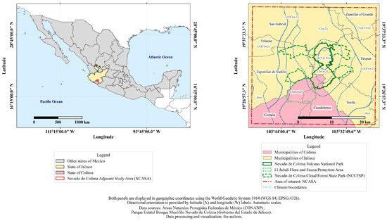
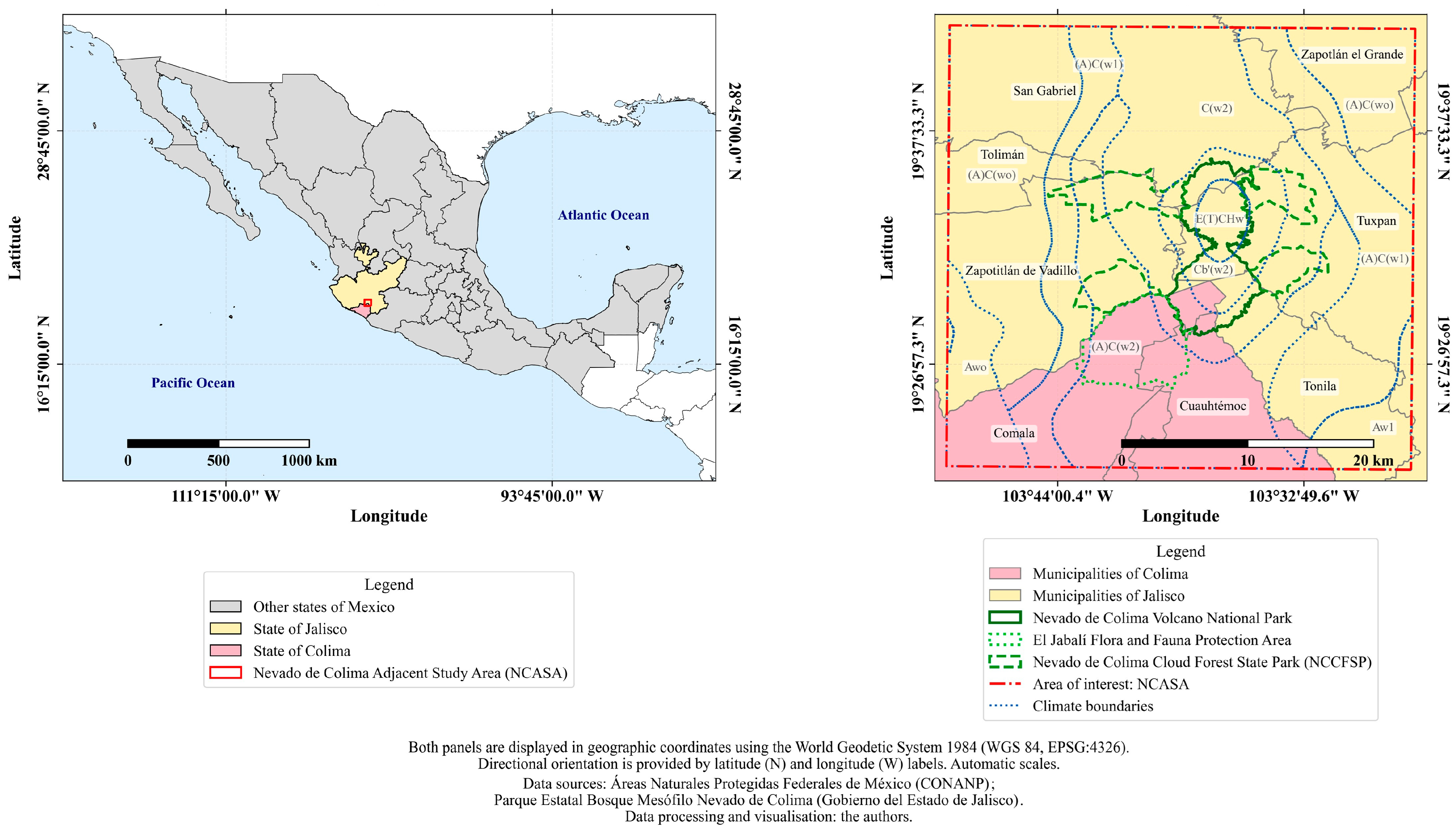
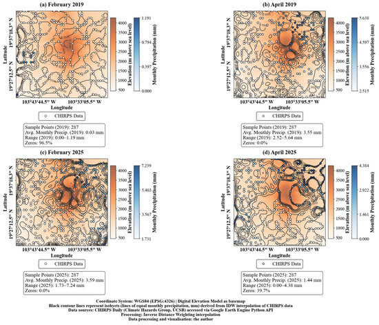
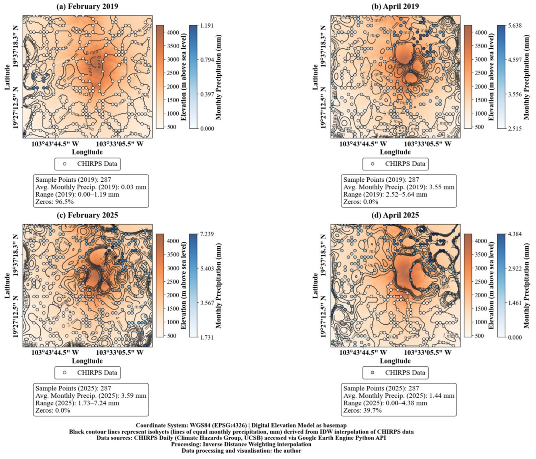
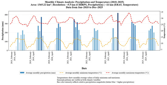
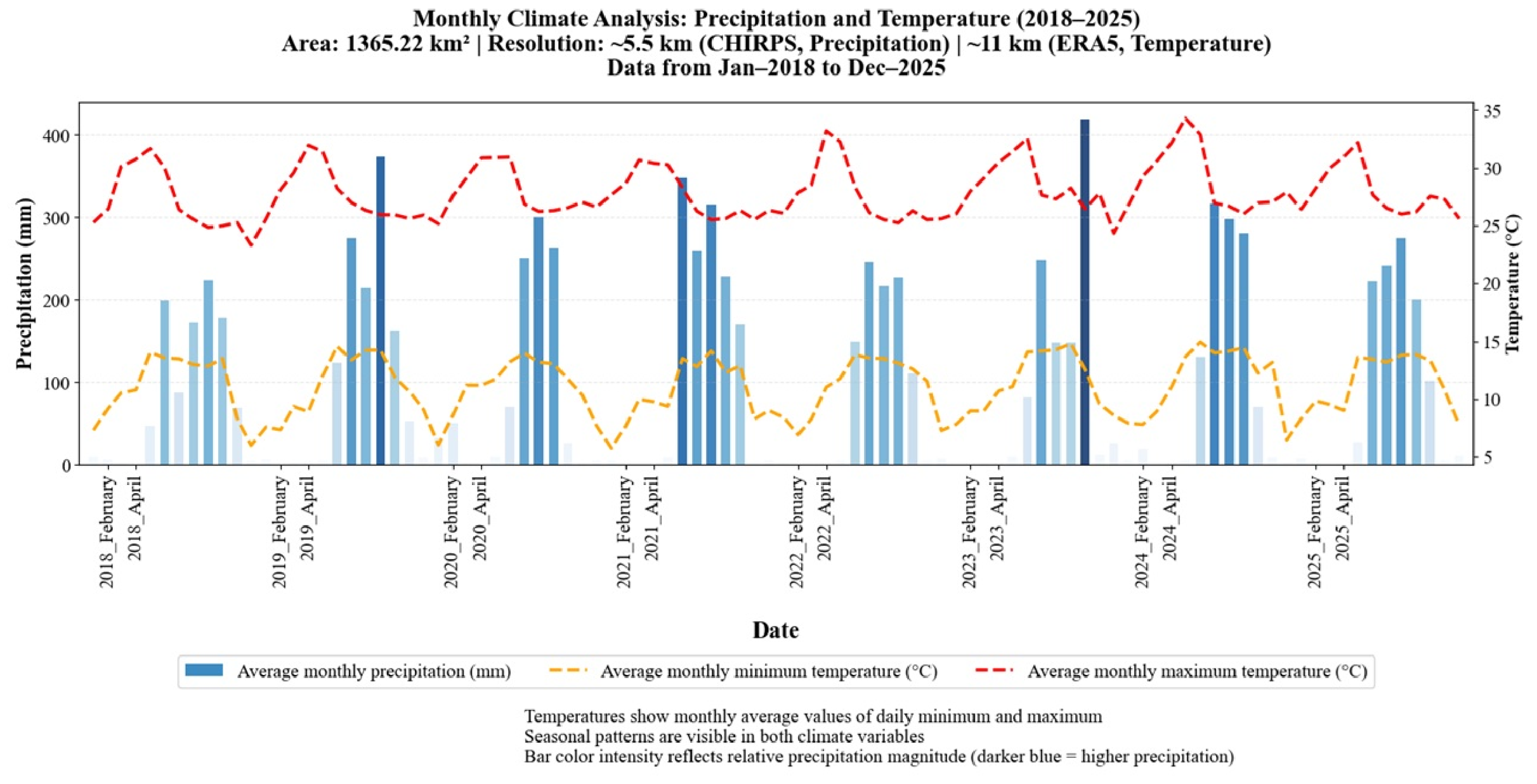
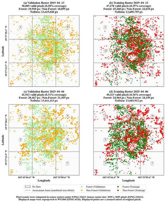
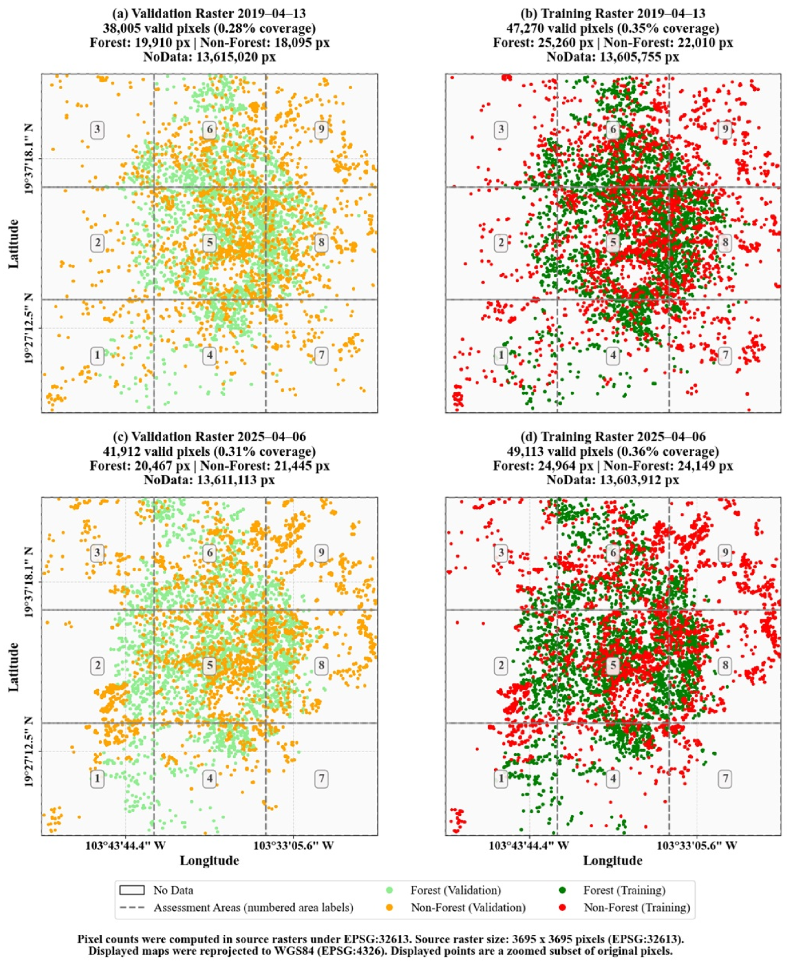
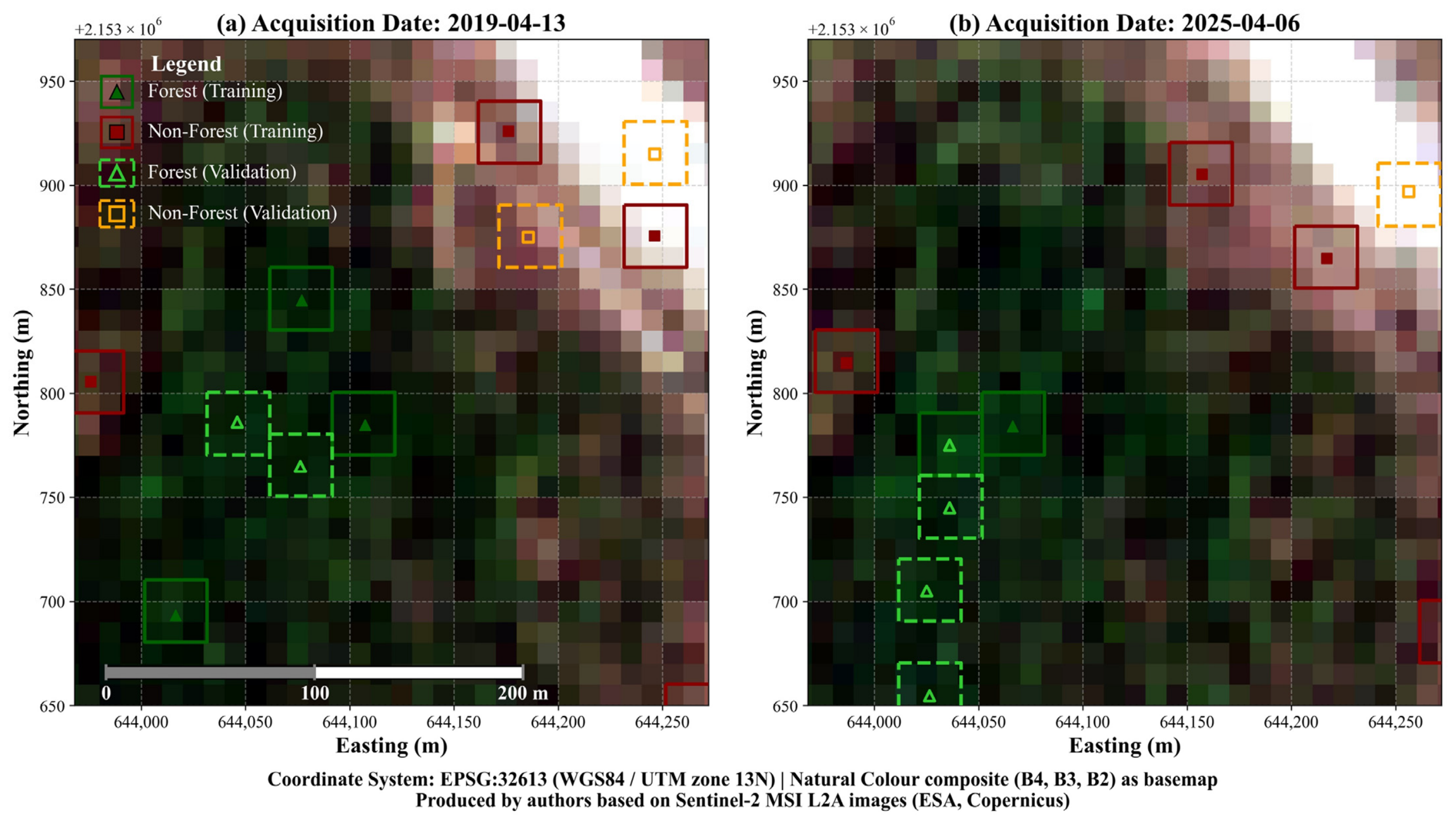
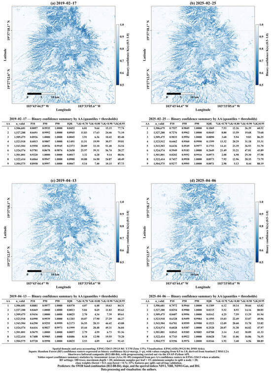
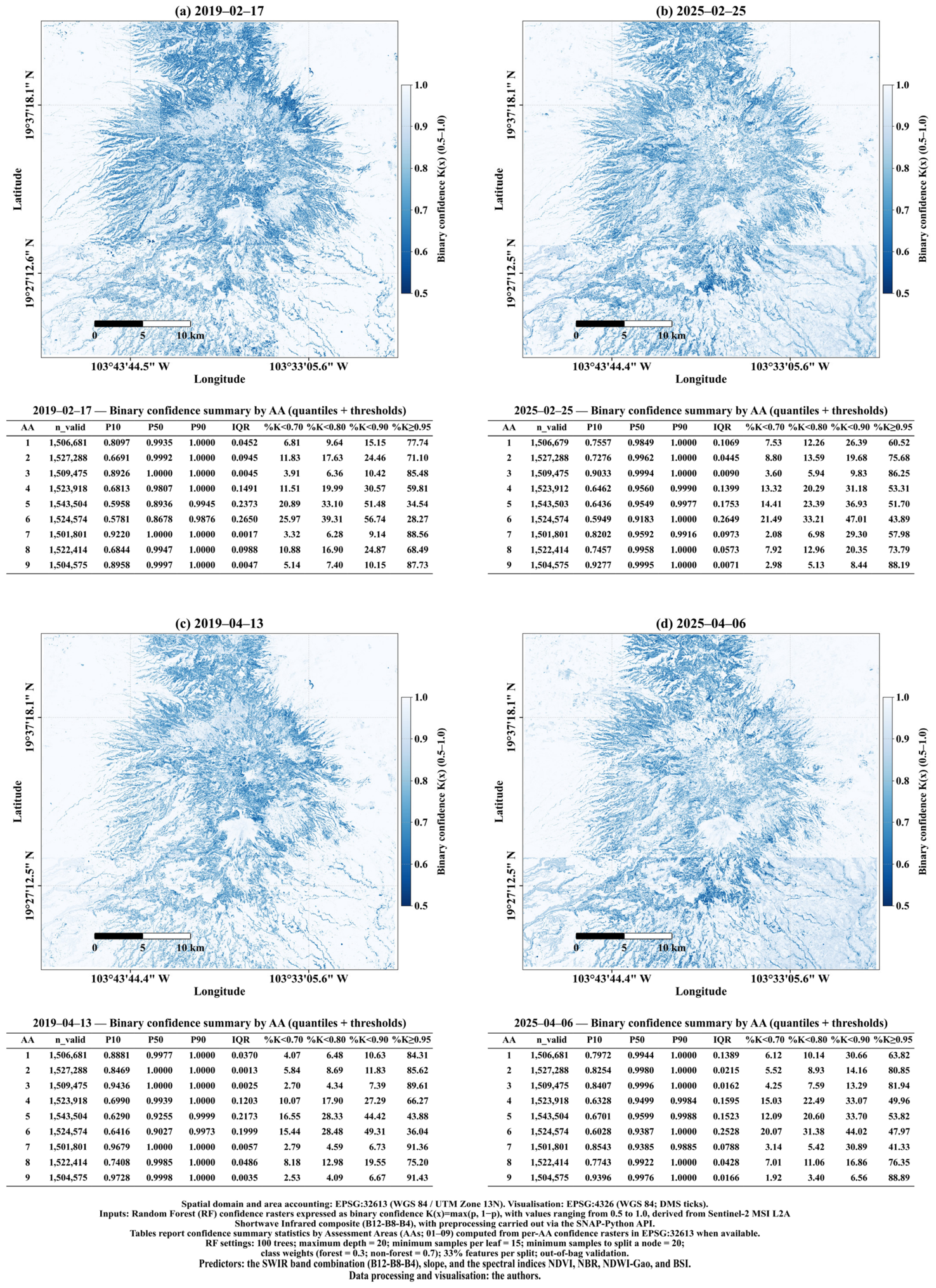
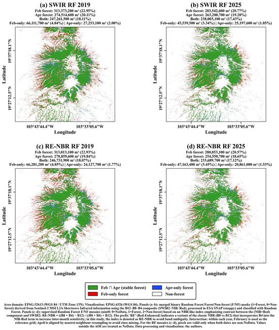
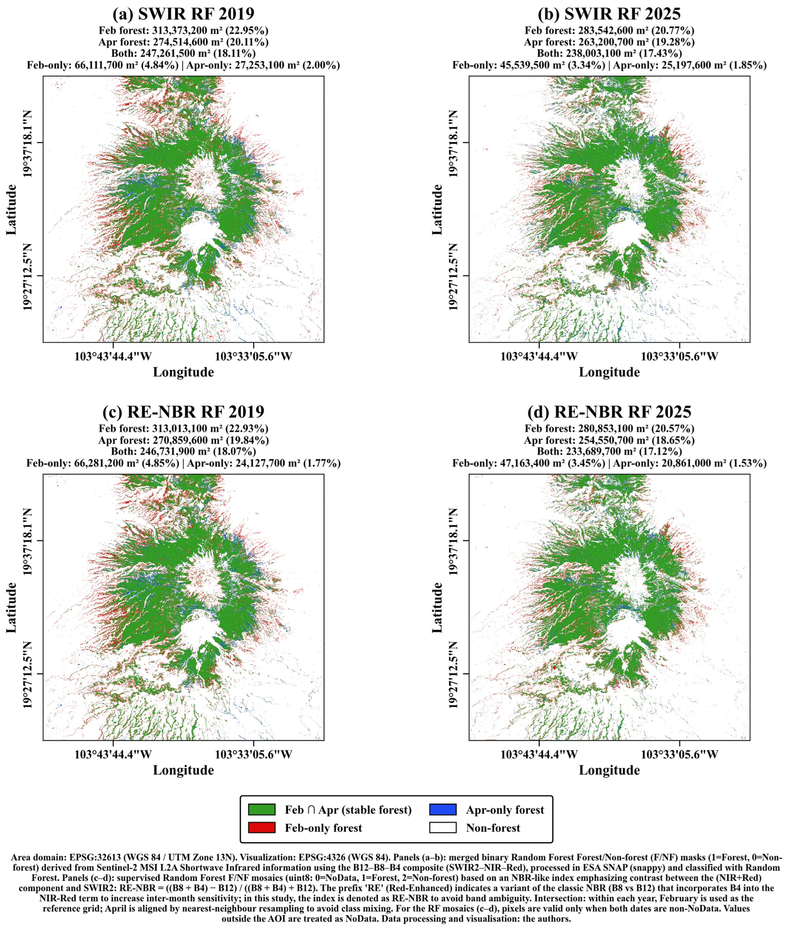
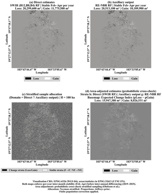
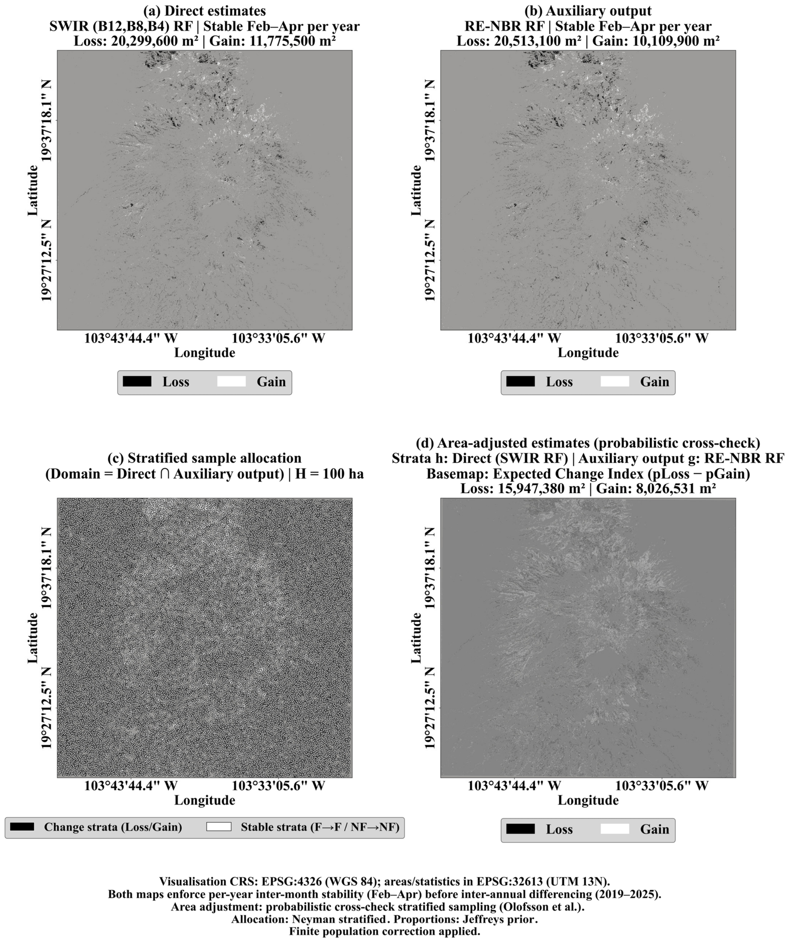
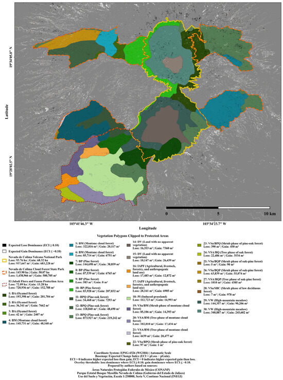
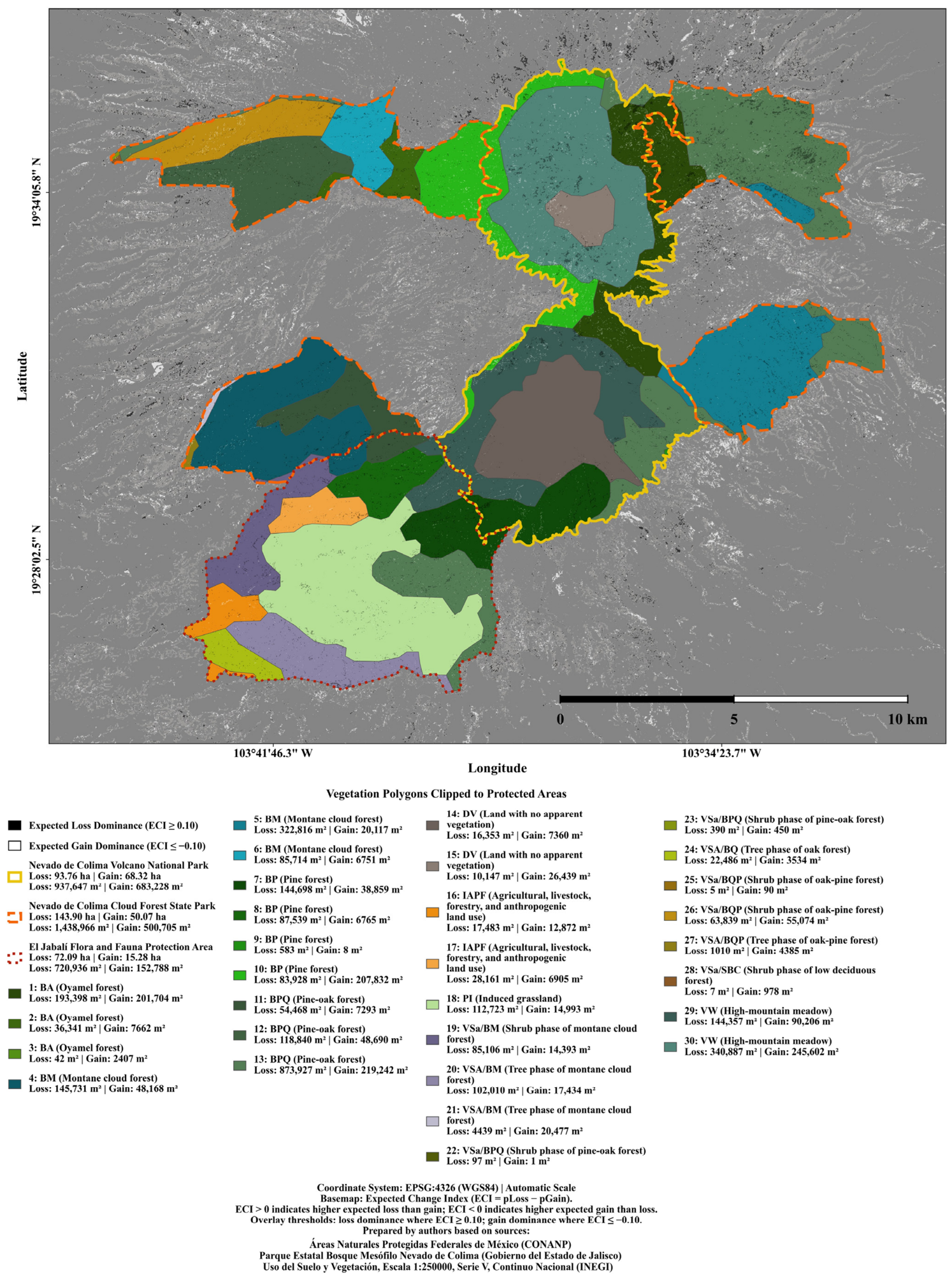

Disclaimer/Publisher’s Note: The statements, opinions and data contained in all publications are solely those of the individual author(s) and contributor(s) and not of MDPI and/or the editor(s). MDPI and/or the editor(s) disclaim responsibility for any injury to people or property resulting from any ideas, methods, instructions or products referred to in the content. |
© 2026 by the authors. Licensee MDPI, Basel, Switzerland. This article is an open access article distributed under the terms and conditions of the Creative Commons Attribution (CC BY) license.