


Abstract
Global warming, which is mainly linked to CO2 increase, has led to a growing interest in assessing carbon conservation in forest biomass. Despite evidence that treelines have advanced by hundreds of meters, knowledge of associated stand biomass changes is insufficient for comprehensive estimation of their role in carbon sequestration. Traditionally, the biomass assessment is based on data collected by field measurements. While this approach provides accurate data for local sites, it cannot be extrapolated properly to larger areas. A more appropriate approach would be to combine field measurements with remote sensing methods. We used data obtained by tree morphometry and annual ring measurements, model-based biomass estimation, processing of laser scanning results, and satellite imagery to model and calculate changes in stand above-ground biomass (AGB) since 1900 at treeline ecotone in Altai and Western Sayan. We developed simulations to predict AGB changes over the coming four decades in these regions. Our findings revealed that the upslope shift of the treeline ecotone by 58–86 m of altitude over the past century was accompanied by an exponential increase in AGB of stands within the 200–400 m forest–tundra transition zone. This resulted in an AGB increment of 120–139 tons per 100 m of treeline. We expect that stand AGB at the treeline ecotone will become 2.3–3.3 times bigger by 2060. All exposures must be considered when estimating stand AGB within treeline ecotones because there are significant differences in treeline elevation, tree-dominant proportions, and stand structure on different slopes.
1. Introduction
Current global warming (temperature increase of 0.85 °C from 1880 to the present), caused by anthropogenic rise in atmospheric concentrations of greenhouse gases (mainly carbon dioxide), has led to a rapidly growing interest in assessing the carbon cycle in terrestrial ecosystems, especially those dominated by trees [1]. Global warming is expected to continue (possibly by 1–3.5 °C), with the most significant changes occurring in subpolar and mountainous regions of the world. This makes studies of the response of highland biota increasingly important, especially in borderline ecosystems where climatic conditions change rapidly over a relatively short distance compared to cross critical thresholds [2]. As it has already happened in many mountain regions over the last century, the expected warming of a few degrees can cause an additional shift of climatic belts by hundreds of meters in altitude [3]. This will prolong significant structural changes in mountain vegetation, mainly due to the expansion of trees and shrubs in alpine tundra and meadows, which have already been identified by many researchers in recent decades [4,5]. This has led to an increase in afforestation over large areas and carbon sequestration in tree biomass, which further feeds back into the global climate [6].
While changes in mountain forest biomass along elevation gradients have been studied intensively for a long time [7], investigation beyond the upper closed forest line has only begun in the last decade [8,9,10,11]. This is mainly because research in these areas is difficult due to their low accessibility and the short period of time during which fieldwork can be carried out. The traditional method of tree stand surveys is the measurement of several tree parameters (e.g., stem diameter and height, crown diameter, vitality) within limited areas—study (test) plots or transects [12,13,14]. Treeline stand biomass assessment was also based on data collected on test plots disposed on focus mountain slopes [11,15]. Although this approach provides the most accurate data, it is time-consuming and labor-intensive. Furthermore, the total spatial coverage of plots is limited to several hectares. In the heterogeneous topographic and edaphic conditions of the highlands, it is impossible to sample all types of tree stands over the course of the field survey. This means that the obtained results do not provide a comprehensive picture of the situation and cannot be used to extrapolate to a larger area (hundreds or thousands of hectares). This important issue could be addressed more appropriately through a combination of ground-based, LiDAR-derived, and remotely sensed data.
Remote sensing methods, widely used in the last decades, provide an excellent basis for studying the tree stands over large areas and in some cases with daily temporal resolution [16,17,18]. Some spatially delimited studies on estimation of local above-ground biomass (AGB) have been conducted in zonal forest–tundra of northwestern and northern Siberia and Alaska based on very high spatial resolution imagery [19] or hyperspectral field spectrometry [20]. Attempts have been made to estimate the AGB by combining field surveys and remote sensing methods using satellite-derived normalized difference vegetation index NDVI in Alaska for shrubby tundra [21,22] and in northeastern Siberia for Larix cajanderi Mayr stands [23]. Shevtsova et al. [24] established a redundancy analysis model using an extensive archive of Landsat satellite data (NDVI, NDWI (normalized difference water index), and NDSI (normalised difference snow index)) to assess the magnitude and direction of forest–tundra AGB change in central Chukotka over the last few decades. Later, in the same region, Shevtsova et al. [25] used Landsat satellite and field data in a statistical model to map and estimate AGB changes between 2000 and 2017. However, the resolution of satellite images (maximum 0.3–0.5 m pixel−1) is still insufficient for precise (up to 0.05–0.1 m) identification of crowns of individual trees, especially small ones found in the upper part of the forest–tundra ecotone [26,27], which is necessary for an accurate assessment of changes in canopy cover over several years or even decades [28] and requires ground-truthing. For example, on the Polar Ural, Nizametdinov et al. [29] have shown that for accurate modeling and reconstruction of changes in treeline stand structure, it is crucial to validate remote sensing estimates by past and present ground-based measurements.
Recently, unmanned aerial vehicle (UAV) imagery has been used to study the structure of woody vegetation over relatively large areas in the polar and upper treeline [30,31]. Within the spatial limitations of field surveys on test plots and the relatively low resolution of satellite imagery data, the UAV platforms can fill the gap and be applied to the precise study of stand structure [32,33]. The data obtained with their use have a very high spatial resolution (0.05–0.2 m pixel−1) and can be collected relatively quickly (within a few days). Automated photogrammetric processing of aerial imagery makes it possible to produce detailed orthophotoplans and three-dimensional point clouds of the study area. This allows us to obtain relatively accurate information on the geographic position and horizontal size of tree and shrub crowns [34,35,36]. However, the identification of tree height is limited in stands with high canopy cover because the bases of objects and the ground surface are not visible. This makes it impossible to create a high-precision digital elevation model and, therefore, to accurately estimate vertical tree parameters [37].
In recent decades, some treeline studies have started actively to use laser scanning [38,39]. This technology is based on the acquisition of a large number of reflection points with high spatial resolution (0.01–0.03 m) using specialized equipment (LiDAR), which allows the relative position of objects to be determined with sufficient accuracy and all morphometric parameters of individual trees to be assessed, even in dense stands. However, despite all advantages of laser scanning methods, the obtained results still require their verification by direct morphometry measurements on the test plots [40].
In 2008–2010, airborne laser scanning and field tree measurements were applied for prediction of tree biomass in the forest–tundra ecotone in northern Norway [41]. Because the laser dataset had 1.4–6.1 points m−2, the relative RMSEs of obtained data after leave-one-out cross-validation were 8.8%–9.5% for maximum tree height, 18.7%–21.2% for tree AGB, and 16.8%–18.7% for vertical canopy cover on plot level. Recently, model-based estimations of AGB in the treeline ecotone were performed in the southern part of Norway using tree stem diameter and height measurements on the test plots, allometric functions between AGB and tree parameters, and point cloud data obtained from airborne laser scanning (2 points m−2) and digital aerial photogrammetry (55 points m−2) [42].
One of the largest and highest mountainous regions in the central part of Eurasia is the Altai and Western Sayan Mountains, which in its size and orography is comparable to the Alps and the Caucasus. A significant warming (increase in summer air temperature of 1.8–2.4 °C) over the last 60 years has been observed at weather stations located in the highlands of this region [43]. It was the warmest period on a longer time scale, based on tree-ring width chronologies of Larix sibirica Du Tour and Pinus sibirica Ledeb. [44,45,46]. A number of projected scenarios for the end of the 21st century show that climate change will continue in the Altai-Sayan Mountains, in particular summer and winter air temperatures will rise, total winter precipitation will increase, while multidirectional precipitation trends are predicted for the summer period [47]. To date, the highlands of this region have attracted researchers mainly for the study of glacier characteristics and dynamics [48,49], radial tree growth [46,50,51] and treeline ecotone structure and dynamics [52,53]. It was revealed that in response to climate warming, the upper limit of open forests in Altai and Western Sayan has shifted upward by 80–130 altitudinal meters over the past 60 years [43]. Such changes in the upper limit of tree stand distribution could have a strong impact on the carbon sequestration into high-altitude ecosystems of these regions. However, no information on the stand biomass and its changes are available for the treeline ecotone of the Altai-Sayan Mountains.
In order to close the gap in this area of knowledge, we set the following aim, namely to estimated AGB of stands and its changes since 1900 in the transition zone between the closed forests and mountain tundra and meadows on the slopes of three mountain massifs in the Altai and Western Sayan and to predict AGB changes on the study slopes in the coming decades using the developed statistical models and the trends of AGB changes in the last decades. We hypothesize that (1) the AGB of treeline stands and its changes are substantially different on slopes with different aspects, (2) the rapid upslope advance of treeline ecotone in the Altai-Sayan highlands in recent decades has been accompanied by an exponential increase in the AGB of stands, and (3) if climatic changes occur at the same rate as in recent decades and the occupation of open areas by stands continues, the total AGB of tree stands will additionally increase by thousands of tons in the next decades.
2. Materials and Methods
2.1. Study Sites
The studies were carried out at the Kholodniy Belok Ridge (N 50.01–50.05°, E 85.78–85.83°) and Taimenie Ridge (N 49.80–49.86°, E 85.70–85.87°), located in the center of the Altai and Kohosh Ridge (N 51.71–51.81°, E 89.63–89.83°), located in the western part of Western Sayan (Figure 1). The regional climate is extremely continental, influenced by air masses from the Atlantic Ocean throughout the year and the Asian anticyclone in winter. Due to the large size of the Altai-Sayan Mountains, air temperatures and precipitation are unevenly distributed across the territory. The highest mean summer temperatures (16–22 °C) were recorded in the western and southern foothills of the Altai. Air temperatures of 2–16 °C were typical in highlands. The highest annual precipitation (600–900 mm) occurred in the western and northern parts of the Altai. Meanwhile, in the eastern part, the precipitation decreases to 200–300 mm. On the territories near the study area, the mean July temperatures are 16.2 ± 1.2 °C in the intermountain valleys (according to the Ust’-Koksa weather station at 980 m above sea level (a.s.l.)) and 7.1 ± 1.3 °C in the highlands at 2600 m a.s.l. (according to the Kara-Tyurek weather station). The average January temperatures are −20.9 ± 3.8 °C and −16.4 ± 2.5 °C, respectively. Annual precipitation is 497 ± 98 mm in the valleys and 623 ± 90 mm in the highlands.
Figure 1.
Location of the study areas on the Altai-Sayan Mountains: (a) the Kholodnyi Belok Ridge, (b) the Taimenie Ridge; (c) the Kohosh Ridge (1); disposition of study plots, scanned areas, and slope sectors on the Kholodnyi Belok Ridge (2) and the Kohosh Ridge (3).
At the present time, the median open forest boundary elevation is 2042 m a.s.l. on the slopes of the Kholodniyi Belok Ridge, 2030 m a.s.l. on the slopes of the Kohosh Ridge, and 1881 m a.s.l. on the slopes of the Taimenie Ridge [43], but it varies in an interval of +/−100 altitudinal meters. In the treeline stands, Pinus sibirica Du Tour and Larix sibirica Ledeb. dominate. The bedrock under the soil cover consists mainly of greenstone, grey-greenstone, grey siltstone, and mudstone [54]. At the Kholodniyi Belok Ridge under the closed forests on the southern slopes, there are Mollic Umbrisols (dark humus soils), but on the eastern slope there are Dystric Cambisoils (brown forest soils) and on the northern and northeastern slopes there are Podzols [55]. Mountain meadow soils are common under subalpine and alpine meadows on the southern slopes [56]. Beyond the belt of alpine meadows on the colder northern and eastern slopes, the area of alpine meadow soils is significantly reduced and replaced by mountain tundra peat and humus soils. While on the northern slopes, at the upper open forest boundary, forest–tundra peaty podzolic soils form a narrow belt.
2.2. Study Design
In our investigations, in order to estimate actual above-ground biomass (AGB) of stands and its changes in 1900–2060 in zones between the closed forests and mountain tundra and meadows, we integrated (1) ground-based survey on test plots (tree mapping and morphometry measurement, stem boring, and core extraction), (2) tree ring width measurements and reconstruction of stem diameter increase during tree life, (3) research of the relationship between tree stem diameter and AGB and calculation stand AGB on test plots, (4) terrestrial laser scanning of slopes and creation of tree stand maps, (5) development of equations of relationship between canopy cover and actual AGB on test plots, (6) analysis of relationships between data from spectral channels of satellite images and canopy cover on laser scanned area, (7) creation of maps of canopy cover and AGB spatial variation on study areas (see Figure 2).
Figure 2.
Block-scheme of study design.
2.3. Tree and Stand Data Sampling and Calculation
In 2021–2023, a series of 3 to 6 study plots (8 m radius) were established at 2–4 elevation levels on the eastern, southern, northeastern, and northwestern slopes of the Kholodniy Belok Ridge, eastern slope of Taimentie Ridge and eastern, southwestern, and western slopes of Kohosh Ridge (Figure 1). These plots were installed at the upper boundary of sparse tree stands (treeline) (level #1), the upper boundary of open forests (OFB) (level #2), the upper boundary of closed forests (CFB) (level #3) and the closed forests located on 30 altitudinal meters down from the upper closed forest boundary (level #4). In each plot, all saplings taller than 20 cm and all adult trees were recorded (N = 2851 in total). Location (azimuth and distance from plot center), height, stem diameter at the base and at 130 cm (if was available), and two crown diameters perpendicular to each other were measured for each stem. In addition to this, using a Pressler increment borer (Haglöf, Långsele, Sweden) a single tree core was taken at a height of 0–30 cm from trees with a diameter greater than 3 cm at the stem base, and boring height was fixed. Using a hand saw, a disk section from the base of the trunk was taken from every third small tree (<3 cm). In the laboratory, all cores and disks were mounted on wooden holders and cleaned with both a paper knife and a razor blade. All wood samples (N = ca. 2123 in total) were measured on the LINTAB-VI linear stage (F. Rinn S.A., Heidelberg, Germany) to an accuracy of 0.01 mm and cross-dated using the TSAPWin Scientific 4.81c computer program. For cores hitting the pith, the distance to the center of the tree was estimated by fitting a circular template to the innermost curved ring [57]. Trees age was estimated for all the studied trees according to methods developed earlier [11,15].
The stem diameters on the base of all examined trees were reconstructed for each year of their life, considering geometric relations [19,21] and according to the following formula:
where DN is the calculated tree diameter in a given year, RN is the radius of the corresponding annual ring, calculated as the sum of all ring widths from the core of a tree trunk to this ring border, ROTR is the radius of the outer tree ring, calculated as the sum of all ring widths from the pith to the border of the outer ring, and DF is the actual tree diameter measured on the site.
DN = (RN/ROTR) × DF
All collected field data were used for calculation of standard statistical characteristics of tree stands growing on all levels of the studied transects.
Additionally, based on tree location and crown size, data obtained during the field survey we created with use of a SAGA GIS 7.8.2 (Open Source Software, University of Hamburg, Germany) map of tree crown disposition on each plot and calculated canopy cover (in %) excluded overlaps of crowns from the total sum of crown projections [58,59].
2.4. Tree Stand Mapping on Sector of Slopes
Moving in zigzags by foot from treeless tundra and meadows down to closed forests, terrestrial laser scanning (TLS) was carried out with the L-SCAN-2 backpack (Geomatics, Moscow, Russia) on the part of north-western (4.8 ha) and eastern (3.1 ha) slopes of the Kholodniy Belok Ridge and eastern (5.8 ha), southern (4.7 ha), and western (1.9 ha) slopes of Kohosh Ridge. The distance between the passages across the slope was 15–20 m. At the same time, we collected geolocation corrections using the PrinCe i50 GNSS receiver (Shanghai HuaCe Navigation Technology Ltd., Shanghai, China). The L-SCAN-2 equipment included a LiDAR scanner (Velodyne VLP-16, Ouster, San Francisco, CA, USA)) and an Applanix Plateau (a GNSS (Global Navigation Satellite System) sensor and an IMU (Inertial Measurement Unit) sensor) (Applanix, Richmond Hill, ON, Canada). The Velodyne VLP-16 laser scanner has a scanning range up to 100 m.
The configuration of the L-SCAN-2 complex allowed the acquisition of geo-referenced one-minute files in LAS format in the program PosPack MMS 8.4, where each data point has a specific latitude, longitude, and altitude a.s.l. We adjusted the geolocation of the reflection points collected by the laser scanner with use of GNSS-receiver corrections. After that, the RMSE of geolocation determination of reflection points became 2–7 cm. Later, all one-minute files (18–25 million points) were merged into a single file in the Lidar360 v.4.1 (Green Valley International Ltd.), and further processing covered the entire area. Point density was 5000–10,000 per m2. Then, during the pre-processing of the point cloud in this package, the following steps were performed: (1) edge cropping, (2) strip alignment, (3) rarefaction and filtering of points by height (5σ), and (4) point classification. Laser reflection points were classified into two types: points on the ground surface and other higher located points [52]. A digital elevation model (DEM) was constructed from the first type of points. Both the first and second types of points were used to construct a Digital Surface Model (DSM). By excluding DEM data from the DSM, a canopy height model (CHM) was developed, which is an image of tree crowns in TIFF raster format. A raster cell size of 0.1 m was used to generate all three models and the developed TIFF raster.
Next, in QGIS version 3.32, the procedure for extracting the outer contours of the crowns was performed using the “Create Isolines” tool. Segmentation of individual trees was based on the CHM. In the case of closely spaced trees, the separation of their crown projection polygons was performed manually, using the “Canopy Height Model” raster. The segmentation result was formed as a vector polygonal layer in SHP format. Segmentation quality control was performed based on individual tree points obtained from the Lidar360 version 4.1 program, which were visually identified (using the “Vector Editor” tool) from the entire point set.
Using the extracted tree crown contours, QGIS software tools were used to determine the area of individual trees and their heights. Tree heights were calculated based on statistical data (QGIS’s “Zonal Statistics” algorithm) on the distribution of pixel brightness in the canopy height model (CHM) (mean, standard deviation, maximum). In this case, pixel brightness corresponded to the height of the scanned object point above the ground. The maximum pixel brightness was taken as the tree height. Using the same algorithm (the “minimum” parameter), tree height above sea level was calculated from the DEM. The QGIS “Rotated Minimum Bounding Box” algorithm was used to extract crown height and width. The geographic coordinates of the centroids of the tree crown projection polygons were used as the coordinates of the trees themselves.
Finally, we produced a digital map in the form of a polygonal layer of crown contours with attribute information for each tree, including minimal and maximal crown width (m), crown area (m2), height (m), geographic coordinates, and elevation (m a.s.l.) (see examples in Figure 3). Using the geographic coordinates of the test plots, we located them on a map of the scanned area and overlaid the tree crown patterns. After, we estimated canopy cover inside of the area of test plots based on attribute information for each tree (see Figure 3a) and developed an equation of relationship between canopy cover values obtained based on field measurements and LiDAR-derived data (see Figure A1). Using this equation, we recalculated canopy cover for all test plots disposed out of the scanned area.
Figure 3.
Tree stand map of the western slope of Kohosh Ridge created based on data from laser scanning and segmentation of tree crowns (brown spots) with overlaid counters of test plots (hatched circle with crown patters obtained based on field measurements) (a) and tree stand map of the eastern slope of Kholodny Belok Ridge (Goggle Earth satellite image) presented in form of blue contours of crowns and divided into 10 × 10 m polygons (brown grid cells) (b).
Each scanned area was divided in 20 m width stripes, where mean elevation, canopy cover, and mean tree height were calculated. Later, in the QGIS software environment, we virtually divided the entire area of the scanned slopes into 10 × 10 m grid cells (polygons) (see Figure 3b), the boundaries of which coincided with the pixel boundaries of satellite images of the Sentinel-2 with a spatial resolution of 10 m pixel−1 made in July and September 2021. The crown projection area of the trees located in these squares were then summed, and canopy cover (in %) was calculated for each grid cell.
2.5. Estimation of Tree Stand Biomass
A total of 18 Siberian pines and 17 Siberian larches were harvested and examined in open forests close to the test plots to cover the full range of stem diameters revealed during field measurements at slopes of Kholodniy Belok and Kohosh Ridges. We selected healthy trees without obvious signs of previous damage to their trunks or crown. By dividing the harvested trees into stem wood and bark, branch wood and bark, and needles, the biomass of the model trees was determined [11,15]. The fresh mass of the stems was assessed by cutting them into 1 or 2 m sections, which were weighed to an accuracy of 50 g. The percentage of dry matter in this wood and bark fraction was determined from cross-cuts from the butt end of the sections, which were weighed to an accuracy of 0.1 g. All branches were cut and divided into three sub-fractions according to their position in the crown (upper, middle, or lower). After measuring the total fresh mass of each sub-fraction in the field, the crown was separated into parts with or without needles and weighed separately. Needles were removed from the branches. A sample of the foliage part (20%–30% of the total fresh crown mass) was weighed. A sample of the foliage-free part (5%–10% of the total fresh crown mass) was used to determine the proportion of wood and bark in the branches. The dry matter content of the foliage was determined on 20 g samples from each part of the crown. All obtained field samples were transported to the laboratory and dried in an oven to an absolutely dry state. After, we weighted these samples and calculated shrinkage coefficients. Based on data of fresh mass of each part of the tree and shrinkage coefficients, we calculated the mass in an absolutely dry state. Finally, we summed the mass of all fractions and estimated the above-ground biomass of each model tree.
By applying regression equations relating the above-ground biomass (kg tree−1) to the diameter at the stem base or breast height (cm), tree height (m), and area of crown projection (m2), relationships were defined. Using functions of the program Origin Pro 2018, we revealed that they are best fitted by the allometric function (y = a × xb). We found that these functions between stem diameters on the base of trees, growing within the treeline ecotone on Altai and Western Sayan, are very similar (R2 = 0.95). Based on that, we merged the data of two regions and fitted the allometric function (Figure 4).
Figure 4.
The dependence of above-ground biomass (AGB) on stem diameter on base (Dbase) for full band of Pinus sibirica (a) and Larix sibirica (b) growing in the treeline ecotone on the slopes of the Kholodny Belok (CHB) and Kohosh (KOH) Ridges.
Parameters of these functions had a high level of confidence and high value of R-Square (0.980 and 0.983), RMSE (13.0 and 19.1), and relative RMSE (13.4 and 17.4%) for both species. As it can be seen in Figure 4, all field reference data are disposed inside of the predicted band of AGB. These results allowed us to use these equations for calculation with high-accuracy AGB of separated trees and actual stand AGB on the test plots.
Using functions of the program Origin Pro 2018, we investigated relations between actual AGB (t ha−1) and canopy cover (%) on the test plots. We found that the allometric function (y = a × xb) is best fitted to that relationship (see Figure 5). Parameters of these functions for each studied transect had high levels of confidence and high values of R-Square (0.938–0.975), RMSE (5.95–13.45), and relative RMSE (13.6%–19.8%). As it can be seen in Figure 6, most of the field reference data are disposed inside of the predicted band of AGB.
Figure 5.
Relationship between stand AGB and canopy cover calculated based on LiDAR-derived data on test plots installed on eastern and southeastern (a), northwestern and northeastern slopes (b) of Kholodny Belok Ridge, eastern (c) and southern and western slopes (d) of Kohosh Ridge.
Figure 6.
Changes in AGB (in % from actual in 2022) of tree stands in forest–tundra transition on the northwestern (NW) and eastern (E) slopes of Kholodny Belok Ridge and on the southern (S) and eastern (E) slopes of Kohosh Ridge on different elevation levels: 1—upper sparse tree stand boundary; 2—upper open forests boundary; 3—upper closed forest boundary; 4—closed forests located 30 altitudinal meters down from the upper closed forest boundary.
The residuals corresponding to the equations shown in Figure 5 were examined for spatial autocorrelation using Moran’s index [60]. On the S and E slopes of the Kholodniy Belok Ridge, Moran’s index was −0.088 (p-value = 0.286); on the NW and NE slopes, it was −0.076 (p-value = 0.456). On the Kohosh Ridge, Moran’s index was 0.003 (p = 0.158); on the NW and NE slopes, it was −0.075 (p = 0.38). These results suggest that the residuals do not exhibit spatial autocorrelation in any of the cases examined.
Based on the distance (in meters) between the elevation levels of the study transects and the AGB of the stands (t ha−1) at these levels, we calculated the AGB for four parts of each slope. To do this, we averaged the AGB value (t ha−1) between levels and multiplied it by the area of that part of the transect (ha). The first part was related to the area between the boundary where the last single tree in the tundra can still be met (where AGB is mostly close to 0) and the boundary of the sparse tree stand (level #1 of transects); the second part was related to the area between levels #1 and #2; the third part was related to the area between levels #2 and #3; and the fourth part was related to the area between levels #3 and #4. By summing the AGB of tree stands within all parts, we calculated the total AGB of stands for the full length of the study transect along the slope (217–400 m). Since the width of the transects varied from 140 to 200 m, we recalculated the AGB per 100 m of their length across the slope. This enabled us to compare the values obtained for the study transects in one or more regions or estimated using other methods.
Similar to how it was applied in our investigations of biomass changes on the Urals, the Kolar Peninsular, and the Putorano Plato [9,11], these equations (see Figure 4) were combined with actual (in 2022) or reconstructed stem base diameter data to estimate AGB on an area basis (ha) for all elevation levels of studied transects at the present time (actual) and for each year since the start of stand establishment at these levels. Finally, we divided the AGB value in each calendar year by the AGB in 2022 (100%) and calculated the corresponding percentage increase of biomass from 1900 to the present (see Figure 6).
Then, for 2000–2022, the regression equations of the percentage changes in AGB by relative years, when 2000 is 101 and 2022 is 123, were obtained for each elevation level (Table 1). The linear type of regression equation was chosen because it reflects the average trend of changes for all elevation levels, whereas the polynomial or power type greatly overestimates the calculated values for the lower levels, where the density of stands has not increased in recent years and may decrease in the future due to higher mortality among old trees.
Table 1.
Parameters of linear equations (y = a + bx) modeling stand AGB changes in 2000–2022 (in % of AGB in 2022) in the treeline ecotone at the Kholodniy Belok (CHB) and Kohosh (KOH) Ridges.
The linear regression model represents a neutral scenario of possible AGB changes, since the expected increase in temperatures in the future may not necessarily lead to improvement of conditions for the emergence and growth of trees, but in the absence of a trend towards an increase in summer precipitation or even a decrease, which has been observed in recent decades, it could contribute to an increase in the frequency and duration of dry periods in summer and thereby deteriorating conditions for tree growth.
Based on developed equations, we calculated how the AGB could increase in relation to the AGB in 2022 at each elevation level in 2022–2060.
2.6. Estimation of Modern Canopy Cover of the Tree Stands Using Satellite Images
Investigation of actual spatial variation of canopy cover on the entire study area was based on 12 bands of Sentinel-2 satellite images with spatial resolution 10 m pixel−1 made in July 2018–2019 and September or November 2021. The July and September images were used under the assumption that surface reflectance values in corresponding pixels of grasslands and tundra sites usually change from summer to autumn, but the ones of forest pixels will have similar values. The obtained results in previous studies revealed the benefit of a multi-temporal analysis of multispectral Sentinel-2 data, since it also addresses seasonal changes in the acquired data [61,62].
In SAGA GIS (University of Göttingen, Germany), we developed equations of relationships between data from 12 spectral channels of Sentinel-2 satellite images, Enhanced Vegetation Index (Summer images), Aspect (independent variables), and canopy cover data in 10 × 10 m grid squares derived from laser scanning (see examples in Figure 7) in 677 locations on the Kholodniy Belok Ridge and 1051 locations on Kohosh Ridge (dependent variables) accompanied by data from test plots (manual measurements) and additional data of sites (10 × 10 m) outside the laser scanned area, which were without trees or fully covered by tree crown (CC value equals 0 or 100%, respectively). Additional data were obtained by means of visual estimation of canopy cover in 2021–2023 satellite images from Google Earth Pro 7.3.6.10441 with resolution 0.5–1.0 m pixel−1. It was performed for increasing the CC range up to as maximal as possible and improving results of regression analysis. We are aware that discrepancies between the size of the test plots and the resolution of the satellite images could distort the assessment of canopy cover. An 8 m radius plot has an area of approximately 200 m2, whereas one pixel has an area of 100 m2, meaning that one pixel cannot fully represent the plot. Sampling values at the plot center risks producing non-representative data and could introduce noise into the training dataset. Orthorectification errors in Sentinel-2 datasets in rugged areas (e.g., mountain sites) could displace pixels by up to 10 m, which can also affect the training datasets. However, after providing feature selection using the stepwise backward elimination method and constructing a multiple regression model to calculate CC, we found that the parameters obtained from these regressions of each studied region had high levels of confidence (see Table A1 and Table A2) and high values of R-Square and RMSE (Kholodny Belok Ridge—R2 = 0.73, RMSE = 12.6, Kohosh Ridge—R2 = 0.58, RMSE = 9.2). When we constructed the regression model, validation was performed using the cross-validation procedure in SAGA GIS (Kholodny Belok Ridge—CV samples = 10, CV R2 = 0.69, CV RMSE = 14.1. Kohosh Ridge—CV samples = 10, CV R2 = 0.57, CV RMSE = 9.2). The visually interpreted Google Earth points were included in both model fitting and validation sets. The cross-validation was not spatially structured. The spatial auto-correlation was controlled in the SAGA GIS module: Kholodniy Belok Ridge—Moran’s I (residuals) = 0.008, Geary’s C = 0.469; Kohosh Ridge—Moran’s I (residuals) = 0.0006, Geary’s C = 0.751. These index values together confirm no significant spatial dependence.
Figure 7.
Disposition of points used for regression analysis with deriving of canopy cover values by manual measurements on the test plots (Manual), LiDAR scanning (LIDAR), and visual estimations (Visual).
Using these regression equations and data from the spectral channels of the Sentinel-2 images, a raster maps of the spatial variation of CC were produced for 1283.7 ha of the eastern part of the Kholodnyi Belok Ridge and 634.3 ha of the southeastern part of the Kohosh Ridge (Figure 8). We consider that extrapolating CC data obtained on the LiDAR-scanned areas to the entire slope sections was reasonably feasible. Firstly, this was due to the relatively large size of these polygons (from 1.9 to 5.8 hectares), whereas a minimum area size of 0.4–0.6 hectares is typically required for stable estimates and reliable extrapolation [63]. Secondly, the scanned area covered all types of tree stands in terms of crown density, ranging from extremely sparse and low-growing to dense and tall, and dominant species composition, which was also typical of areas outside the scanned zones [64]. Thirdly, the automatic extraction of crown contours from a high-density reflection point cloud (5000–10,000 points per m2) was sufficiently accurate (±0.1 m) and visually verified additionally. This ensured that the projected areas of individual tree crowns and CC of the stands were estimated as realistically as possible.
Figure 8.
Actual canopy cover of tree stands on Kholodny Belok and Kohosh Ridges.
In the SAGA GIS 7.8.2 software, using the supervised classification method, we divided the study area based on attributive data of each raster of the actual CC map into the polygons with different canopy cover type: 1—0.1%–5%; 2—6%–20%; 3—21%–40%; 4—41%–55%; 5—56%–75%; 6—>75% (Figure 9). This division into types was based on a statistical analysis of canopy cover in the test plots established at different levels (1–4) of elevation transects in all study areas (see Figure A2). Additionally, in the QGIS software environment, using a digital elevation model (NASA Shuttle Radar Topography Mission 2013), we divided the study areas into sectors (S, SW, W, SE, E, NE, NW) according to the slope exposure (see Figure 8 and Figure 9).
Figure 9.
Map of the polygons with different types of canopy cover in 2022: 1—0.1%–5%; 2—6%–20%; 3—21%–40%; 4—41%–55%; 5—56%–75%; 6—>75%. Blue lines divide the territory in sectors of different exposition: W—western; NW—northwestern; NE—northeastern; E—eastern; SE—southeastern; S—southern; SW—southwestern. Position of open forest boundary in 1960s demonstrated by mean of dotted line (OFB 1960).
2.7. Calculation of ABG of the Tree Stands on the Study Areas
In the SAGA GIS software environment, using attributive data of each raster cell of the digital map of the spatial variation of canopy cover in 2022 (Figure 8) and the relationship between AGB and canopy cover (Figure 5), we calculated AGB in each raster cell and created a map of the actual spatial distribution of AGB (see the corresponding figures in Results). After, we reconstructed year-to-year AGB changes in 1900–2022 in each raster cell of this map, according to calculated biomass changes (in %) on the test plots of different elevation levels of the studied transects (Figure 6). For calculation of AGB changes in the next decades, we used attributive data of the AGB map in 2022 and regression equations of the AGB changes (in %) in the period between 2000 and 2022 (see Table 1).
Finally, we calculated the total AGB within polygons with different canopy cover types (0.1%–5%, 2nd—6%–20%, 3rd—21%–40%, 4th—41%–55%, 5th—56%–75%) into each sectors (S, SW, W, SE, E, NE, NW) of the study area (Figure 9) using the AGB values of raster cells of digital maps created for 1920, 1960, 2022, and 2060. Such operation was conducted only for polygons, which are disposed above the virtual line located 80 m below the low border of polygons with CC of 41%–55%.
By summing the total AGB of stands of all types of polygons in slope sectors, we calculated the total AGB stock in each sector (S, SW, W, SE, E, NE, NW). Since the treeline length in sectors varied from 1.62 to 3.4 km on Altai and from 0.93 to 2.16 km on Western Sayan, we recalculated the total AGB of the stands per 100 m of treeline length. This allowed us to compare results obtained for different sectors and between studied regions.
2.8. Estimation of the Length of the Treeline on the Territory of the Altai Republic
Additionally, on the territory of the Altai Republic, we estimated the length of the upper boundary of the areas dominated by trees with a cover of more than 10% (tree covered area—TCA) based on a classified raster obtained from the ESA WorldCover global coverage using the Google Earth Engine service [65]. The following object classes without woody vegetation (snow and ice, moss and lichen, bare/sparse vegetation, and grassland) were extracted from this raster. To facilitate the processing procedure, the resolution of the ESA WorldCover raster was decreased from 10 m to 50 m per pixel. Vectorization of the final raster was performed in the SAGA GIS environment [66]. Additionally, the boundaries of the resulting polygons were simplified using the SAGA GIS Line Simplification module (tolerance 50). These were then converted into points with a 100-m interval. Next, based on high-resolution images from the World Imagery servers (ESRI, USA), polygons were created that included only the upper boundaries of TCA (see Figure 10). The points of the boundaries of the TSA located in the lower part of the mountain slopes were removed, and the remaining ones were used to estimate the extent of such boundaries in the Altai region, which most closely match with the upper boundary of sparse tree stands (treeline) on level #1 of the studied transects or the type of polygons with CC 6%–20%.
Figure 10.
Polygons separating the upper treeline from other forest boundaries (blue lines) and the ESA WorldCover layer reflecting treeless areas (red) on the territory of the Altai Republic.
3. Results
3.1. Modern Structure and Biomass of Treeline Stands
Analysis of the structure of stands growing on slopes of the Kholodny Belok, Taymentie, and Kohosh Ridges shows that mean age reduced by 2.5–3 times from low to upper parts of elevation transects (Table 2 and Table 3). Thus, larch age, averaged for all plots, decreased from 210 ± 73 years at level #4 to 133 ±67 years at level #3, to 87 ± 32 years at level #2, and to 68 ± 22 years at level #1. At the same time, the pine age declined from 108 ± 56 years at level #4 to 72 ± 27 years at level #3, to 52 ± 20 years at level #2, and to 42 ± 18 years at level #1.
Table 2.
Morphometric (mean ± s.d.) and areal characteristics of the studied tree stands on the Kholodny Belok (CHB) and Taymenie (TAI) Ridges on the Altai Mountains.
Table 3.
Morphometric (mean ± s.d.) and areal characteristics of the studied tree stands on the eastern part of the Kohosh Ridge on the Western Sayan Mountains.
We also found that tree morphometric parameters (stem diameter, height and crown diameter) decreased by a factor of 2–6 (Table 2 and Table 3). Thus, average height of larches decreased from 14.3 ± 3.9 at level #4 to 10.4 ± 4.2 at level #3, to 7.1 ± 3.9 at level #2, and to 5.4 ± 1.3 at level #1. But average height of pines reduced from 7.7 ± 3.9 at level #4 to 6.0 ± 2.9 at level #3, to 3.8 ± 1.9 at level #2, and to 2.3 ± 0.7 at level #1. Analysis of areal characteristics (canopy cover, stand density) demonstrated that they decrease by a factor of 5–10 with increasing altitude (Table 2 and Table 3). Thus, canopy cover, averaged for all test plots installed at level #4, was 59.9 ± 8.2%, for level #3—47.7 ± 5.2%, for level #2—36.2 ± 9.4%, and for level #1—10.9 ± 3.4%.
Analysis of data on tree height and crown size obtained by processing the results of laser scanning (using LiDAR) of 80–100 by 300–500 m sections on the E and NW slopes of the Kholodny Belok Ridge showed that in the upper part of these areas, the canopy cover increased gradually downslope from 0.2 to 4%–8% and then sharply enlarged by 3–4 times to 15%–19% (see Figure 11). Further downslope, after 35–50 m of altitude, the canopy cover again increased sharply by a factor of 2 to 35%–55%. In 20 m strips with an average canopy cover of 8%–15%, and the average height started to exceed 2 m and then increased smoothly to 8–10 m towards the lower part of the scanned areas. At the same time, the maximum height of trees gradually increased from 2–2.5 m in the upper part to 15–17 m in the lower part of the scanned territories. A similar pattern of changes of canopy cover and mean tree height was marked on scanned slopes of Kohosh Ridge (see Figure 11).
Figure 11.
Changes of canopy cover with altitude on laser scanned parts of northwestern (1) and eastern (2) slopes of Kholodny Belok Ridge and eastern (3) and southern (4) slopes of Kohosh Ridge.
It was also found that the rate of AGB change with altitude varies on slopes with different exposures. Thus, the canopy cover decreases by a factor of 22.5 on the E slope and by a factor of 48.4 on the N slope of Kholodny Belok Ridge. The ratio of pine to larch by AGB also differs significantly on slopes with different exposures (see Table 4). Thus, the total AGB of larches is higher than that of pine on the E slope (53–63 vs. 37%–47%) and lower than on the N and S slopes (0–53 vs. 47%–100%) of Kholodny Belok Ridge. On the northeastern slope, however, larch is almost absent on the upper level (#1) and dominates in closed forests (level #4) (68%). But, on most of the elevations of the treeline ecotone on the E slope of the Taimenie Ridge and S slopes of the Kohosh Ridge, larches prevail (52–98%) (Table 4). In opposition, on the E slopes of this ridge, Siberian pine dominates (92–100%).
Table 4.
Mean portion (%) of pine and larch biomass in total AGB of stands on plots on different elevation levels and slope of Kholodny Belok (CHB), Kohosh (KOH) Ridges, and Taimenie (TAI).
3.2. Changes in AGB on Parts of Slopes Studied with Ground-Based Methods
Reconstructions based on field measurements of stand AGB on test plots of elevation transects installed on the eastern and northern slopes of the Kholodny Belok Ridge (Altai Mountains) and the Kohosh Ridge (Western Sayan) show pronounced changes over the last few centuries (see examples in Figure 12). Thus, at level #4 on the eastern slope of the Kholodny Belok Ridge (CHB), stand AGB, which is 150.8 t ha−1 at the present time, had a similar AGB as those at level #1 (6.7 t ha−1) in 1931. In 1957, the stand biomass on this level already corresponded to the actual biomass on level #2 (25.9 t ha−1), and, in 1995, it had similar values as on level #3 (90.8 t ha−1) at present. At the upper boundary of the closed forest (level #3), the stand biomass corresponded to the AGB values observed today at level #1 in 1977 and at level #2 in 1994. In 1998, the AGB on level #2 was equal to the AGB values observed on level #1 at the present time.
Figure 12.
Changes in AGB of stands on test plots on the northwestern (NW) and eastern (E) slopes of Kholodny Belok Ridge and on the southern (S) and eastern (E) slopes of Kohosh Ridge on 1—upper sparse tree stand boundary; 2—upper open forests boundary; 3—upper closed forest boundary; 4—closed forests located 30 elevation meters down from the upper closed forest boundary.
Due to the earlier start of tree occupation of the northwestern slope of the CHB (mean age of larch is 370–380 years), on plots of level #4 (actual AGB is 251.6 t ha−1), stands have already accumulated similar biomass as at level #1 (5.2 t ha−1) in the 1680s (Figure 1). The stand biomass on this level was the same as on level #2 (70.7 t ha−1) in 1855 and on level #3 (92.4 t ha−1) in 1906. At the modern upper boundary of closed forests (level #3), stands already had AGB as high as at the sparse stand boundary (level #1) in 1733 but only reached similar values as at level #2 in 1994. At the upper boundary of open forests (level #2), stand biomass in 1980 was similar to that observed at level #1 at the present time.
On the eastern slope of the Kohosh Ridge (KOH), the age of the oldest trees is more than 300 years at plots on level #4, and therefore stand AGB, which is 152.8 t ha−1 at present, was already similar to those at level #1 (3.6 t ha−1) in 1760 (Figure 12). In 1940, the biomass on this level was already related to the actual biomass on level #2 (42.7 t ha−1), and in 1995, it had similar values to the actual biomass on level #3 (104.5 t ha−1). At the contemporary closed forest line (level #3), the stand biomass in 1945 corresponded to the AGB values observed today at level #1 and in 2001 at level #2. The AGB on level #2 in 1975 was equal to the modern AGB values observed on level #1. Because mean larch age is 91 years at plots on level #4 on the southern slope of the KOH, stand AGB, which is 97.0 t ha−1 at the present time, was already similar to those at level #1 (4.9 t ha−1) only in 1970 (Figure 12). In 1994, the biomass on this level already related to the actual biomass on level #2 (28.3 t ha−1), and in 2010, it had similar values to the actual biomass values on level #3 (57.4 t ha−1). At the contemporary closed forest line (level #3), the stand biomass in 1976 corresponded to the AGB values observed today at level #1 and in 2010 at level #2. The AGB on level #2 in 1997 was equal to the modern AGB values observed on level #1.
For the reason that the widths of transects varied from 140 to 200 m, we calculated total AGB per 100 m of treeline length across slope for easier comparison with data received by other methods. As a result, our calculations of total AGB on low parts of the study transects between levels #3 and #4 on the Kholodny Belok Ridge (Figure 13) showed that it has increased since 1920 on 64.8, 90.1, and 118.6 t 0.1 km−1 of treeline on the E, NE, and NW slopes, respectively, reaching 66.1, 104.6, and 197.6 t 0.1 km−1 at present. We assume that it could additionally increase to 53.2, 88.3, and 133.7 t 0.1 km−1 on these parts of the slopes by 2060. We found that in areas between levels #2 and #3, the AGB has already increased since 1920 to 37.2, 42.7, and 52.9 t 0.1 km−1 on NE, E, and NW slopes, respectively, and has reached 51.2, 42.7, and 68.2 t 0.1 km−1 at present (see Figure 13c,g). By 2060, it is expected to increase further to 73.3, 55.1, and 98.1 t 0.1 km−1. While in areas between levels #1 and #2, the biomass increment was 12.9, 14.2, and 49.9 t 0.1 km−1 on NE, E, and NW slopes and reached at the present time 13.0, 14.2, and 51.4 t 0.1 km−1 (Figure 13b,f). It is expected to increase further to 44.1, 51.5, and 83.8 t 0.1 km−1 by 2060. On parts of slopes above the upper limit of sparse tree stands, which were almost treeless in 1920, AGB increased to 1.9, 2.3, and 7.2 t 0.1 km−1 on NE, E, and NW slopes, respectively (Figure 13a,e). We expect that in the next 40 years, AGB in these areas will increase further to 5.4, 9.3, and 14.5 t 0.1 km−1.
Figure 13.
AGB changes of tree stands (tons per 0.1 km of treeline length) on study transects on Kholodny Belok Ridge (E—eastern; NW—northwestern, NE—northeastern) and Kohosh Ridge (E—eastern; S—southern; W—western): (a,e) at 1 level with CC 6%–20%; (b,f) between 1 and 2 levels with CC 21%–40%; (c,g) between 2 and 3 levels with CC 41%–55%; (d,h) between 3 and 4 levels with CC 56%–75%.
Our estimations of total AGB on low parts of study transects between levels #3 and #4 on the Kohosh Ridge (right part of Figure 13) demonstrated that it has increased since 1920 to 65.8, 75.6, and 138.5 t 0.1 km−1 of treeline length on W, S, and E slopes, respectively, and reached at the present time 81.5, 75.9, and 171.8 t 0.1 km−1 (Figure 13d,h). We suppose that it will increase additionally to 53.3, 105.6, and 112.4 t 0.1 km−1 on those parts of the slopes. We found that in areas between levels #2 and #3, AGB has increased already since 1920 to 55.3, 44.2, and 73.4 t 0.1 km−1 on W, S, and E slopes, respectively, and reached at the present time 55.6, 44.6, and 73.8 t 0.1 km−1 (Figure 13c,g). We expect that by 2060, it will increase additionally to 70.9, 82.6, and 88.9 t 0.1 km−1. Meanwhile, in areas between levels #1 and #2, stands were absent in 1920, and by the present time, AGB is 25.0, 11.9, and 25.1 t 0.1 km−1 on W, S, and E slopes, respectively (Figure 13b,f). We suppose that it will increase additionally to 49.4, 38.5, and 48.6 t 0.1 km−1 by 2060. On parts of slopes above the upper boundary of sparse tree stands, which were treeless in 1920, AGB increased to 3.2, 3.1, and 1.8 t 0.1 km−1 on W, S, and E slopes, respectively (Figure 13a,e). We expect that in the next 40 years, AGB will increase additionally in these areas to 11.1, 7.5, and 5.7 t 0.1 km−1.
3.3. AGB Changes in Treeline Stands Studied with Ground-Based, Laser Scanning, and Remote Sensed Methods
We mapped the distribution of stand AGB on the slopes of the eastern part of the Kholodny Belok Ridge (CBH) in different years of the period between 1900 and 2060 using a combination of ground-based, terrestrial laser scanning, and remote sensing methods (see examples in Figure 14). We found that the total AGB of stands within polygons with actual CC of less than 5% (tundra with single trees) did not exceed 0.1 tons per 100 m of treeline length (t 0.1 km−1) until 2000 (see Figure 15a). Subsequently, the biomass increased slightly on all slopes and reached 6.0–6.1 t 0.1 km−1 on the S and SE slopes, 3.2 on the E slopes, and 1.5–1.7 0.1 km−1 on the NE and NW slopes at present. We predict that the total AGB in these CC polygons will increase 4.9–9.6 times by 2060, reaching 14.5, 15.3, and 15.9 on the NW, NE, and E slopes and 29.3 and 30.2 t 0.1 km−1 on the S and SE slopes, respectively.
Figure 14.
Spatial distribution of AGB on the slopes of the eastern part of Kholodny Belok Ridge (Altai) in different years: (a) 1920, (b) 1960, (c) 2022, and (d) 2060. The yellow line demonstrates the low border of the study area.
Figure 15.
AGB changes of tree stands (tons per 100 m of treeline length) on different slope aspects of Kholodny Belok into polygons with different canopy cover: (a) 0.1%–5%; (b) 6%–20%; (c) 21%–40%; (d) 41%–55%; (e) 56%–75%.
We found that the AGB of tree stands within polygons with CC of 6%–20% (sparse tree stands) on the CHB was less than 0.1 t 0.1 km−1 until 1960 (Figure 15b). After that, it increased slightly until 2000, after which it began to grow exponentially on all slopes. By 2022, this had led to gains of 4.6–5.2 on E, NE, and NW and 11.7–13.4 t 0.1 km−1 on S and SE slopes, respectively. We expect that in the next 40 years, the total AGB will increase by 4.6–8.3 times. Consequently, it will reach 23.8 on the E, 32.6–37.8 on the NE and NW and 52.6 and 64.1 t 0.1 km−1 on the S and SE slopes, respectively.
At the same time, the total AGB of stands within polygons with CC of 21%–40% (open forests) on the CHB was already 0.5 and 1.1 t 0.1 km−1 on the NE and NW slopes, respectively, in 1920 (see Figure 15c). On the other slopes, the AGB was less than 0.1 t 0.1 km−1 until 1950. By 1980, the AGB had reached 1.1–3.6 t 0.1 km−1 on all slopes. Between 1980 and 2020, the AGB increased significantly by 10–13 times on all slopes. Thus, the total AGB reached 13.2 and 13.8 on the E and NW, 17.1 and 19.6 on the SE and NE, and 35.1 t 0.1 km−1 on the S slopes, respectively, by 2022. We assume that the AGB will increase by 3.8–6.7 times by 2060. Thus, the AGB will be 49.7 and 69.5 on the E and SE, 92.8 on the NW, and 106.1 and 133.6 t 0.1 km−1 on the NE and S slopes.
We found that the AGB of stands within polygons with CC of 41%–55% (closed forests) on the CHB was less than 0.1 t 0.1 km−1 until 1940 on S, SE, and E slopes. However, on NE and NW slopes, AGB was already 3.2 and 3.7 t 0.1 km−1 in 1920 (Figure 15d). Thereafter, there was an exponential increase in AGB on all slopes. By 2022, biomass had reached 17.8 and 20.9 on E and SE, 30.1 and 34.8 on NE and NW, and 52.5 t 0.1 km−1 on S slopes. We predict that AGB will increase 2.8–3.3 times in the next 40 years. As the biomass value varies greatly in different aspects at present, the AGB will reach greatly different values by 2060: 49.0 and 68.5 on E and SE, 91.7 and 106.2 on NE and NW, and 167.1 t 0.1 km−1 on the S slopes.
We estimated that on the CHB within polygons with crown closure 56%–75%, disposed above the virtual line located 80 m below the low border of polygons with CC of 41%–55%, the total AGB was equal to 12.1 and 14.0 t 0.1 km−1 on the NE and NW slopes, respectively, in 1920. On the E, S, and SE slopes, it was less, at 0.2 t 0.1 km−1, respectively (see Figure 15e). The remarkable increase in the AGB started in 1960–1980 on all slopes of this CC polygon type. However, the fastest changes were observed on the NE and NW slopes, where the AGB reached 94.1 and 106.6 t 0.1 km−1 by 2022. Medium AGB values were found for E and S slopes (63.5 and 66.8 t 0.1 km−1, respectively) and minimum values for SE slopes (26.2 t 0.1 km−1). We expect that by 2060, the stand AGB will increase 1.8–2.7 times. As the actual biomass value varies greatly in different aspects, the AGB will reach 217.1 and 238.1 on the NW and NE, 178.2 on the S, 116.4 on the E, and 61.1 t 0.1 km−1 on the SE slopes.
Also, we studied stand AGB distribution on slopes of the Kohosh Ridge (KOH) in different years of the period between 1920 and 2060 (Figure 16) and revealed that the AGB within polygons with contemporary CC less than 5% was close to zero until 2010 (see Figure 17a). Subsequently, the AGB increased slightly on all slopes and reached 0.7–4.0 tons per 100 m of treeline length at present. We predict that the AGB in these CC polygons will increase by 10.7–31.6 times by 2060 and will reach 7.5 and 9.1 on the S and W, 38.7 and 39.6 on the SE and SW, and 126.3 t 0.1 km−1 on the E slopes.
Figure 16.
Distribution of AGB on slopes of Kohosh Ridge in different years: (a) 1920, (b) 1960, (c) 2022, and (d) 2060. The black dash line demonstrates the low border of the study area.
Figure 17.
AGB changes of tree stands (tons per 100 m of treeline length) on different slope aspects of Kohosh Ridges into polygons with different canopy cover: (a) 0.1%–5%; (b) 6%–20%; (c) 21%–40%; (d) 41%–55%; (e) 56%–75%.
We found out that, on the KOH, the AGB of stands within polygons with contemporary CC of 6%–20% was less than 0.1 t 0.1 km−1 until 2000 (see Figure 15b) on all slopes, except on the eastern slope, where it was 3.6 t 0.1 km−1. After, the AGB started to increase exponentially on all slopes and resulted in a gain of 4.7–19.3 t 0.1 km−1 at present. By 2060, we expect that the total AGB will increase 8.8–17.3 times and will be 51.4 and 53.5 on the SW and W, 82.4 and 104.5 on the S and SE, and 261.6 t 0.1 km−1 on the E slopes.
The AGB of stands within polygons with contemporary CC of 21%–40% on the KOH was less than 0.2–2.2 t 0.1 km−1 until 1980 (see Figure 17c). After 2000, there was an exponential increase in AGB on all slopes. Actual biomass reached 11.5 on the W, 17.3, 17.5, and 19.6 on the E, SE, and S, and 53.4 t 0.1 km−1 on the SW slopes. We expect that by 2060, AGB will increase 5.7–13.8 times. Since the biomass value varies greatly in different aspects at present, the mean AGB will reach 84.6 on the W, 149.4 and 176.0 on the S and SE, and 237.9 and 301.5 t 0.1 km−1 on E and SW slopes, respectively.
Our calculations demonstrated that the AGB of stands within polygons with contemporary CC of 41%–55% on all slopes of the KOH was very low (0.1–3.2 t 0.1 km−1) in 1920 (see Figure 17d). By 1980, the AGB had increased by 2.3–13.6 t 0.1 km−1. After that, there was a significant increase of 13–16 times on the SE and SW slopes. Less pronounced changes were observed on the W (7.3 times) and S and E slopes (4.8 times). Thus, by 2022, the AGB was 16.8 and 17.3 on the E and W, 30.3 on the SE, and 65.7 and 73.5 t 0.1 km−1 on the S and SW slopes, respectively. Consequently, it is predicted that the AGB will increase by 2.9–5.2 times by 2060. Thus, the AGB will reach 57.5 on the W, 87.4 on the E, 123.0 on the SE, 187.1 on the S, and 313.5 t 0.1 km−1 on the SW slopes.
We estimated that within polygons with CC of 56%–75%, disposed above the virtual line located 80 m below the low border of polygons with CC of 41%–55%, (see Figure 17e), the AGB was equal to 16.4 t 0.1 km−1 in 1920 on the S slope. At the same time, on others slopes, it was 0.6–3.4 t 0.1 km−1. The stand AGB increased during the last 100 years on all slopes of this CC polygon type. However, the S slope experienced faster changes, where the AGB reached 148.0 t 0.1 km−1 in 2022. Medium AGB values were found on the W and SW slopes (19.4 and 58.6 t 0.1 km−1, respectively) and minimum values on the E and SE slopes (6.4 and 8.1 t 0.1 km−1, respectively). We expect that the AGB of these stands will increase 2.2–2.7 times by 2060. As the biomass value varies greatly in different aspects at present, the AGB will be 14.8 on the SE, 20.7 on the E, 43.2 on the W, 161.4 on the SW, and 318.8 t 0.1 km−1 on the S slopes.
The practical reason for conducting this study was the need to assess the contribution of changes in the ABG of treeline stands to the overall carbon budget of the studied regions. According to estimations of Robertus et al. (2014), the total reserve of organic carbon in the above-ground biomass of the forested area of the Republic of Altai amounted to 311 million tons [67]. Taking into account that AGB contains an average of 50% carbon, the total AGB of forests in the Republic of Altai is 622 million tons. If we take into account that the length of the treeline in the Altai Republic according to our estimates with use of the ESA WorldCover global coverage is about 20,000 km, then over the past 100 years in this region, the total biomass of trees near the treeline has increased possibly by about 24 million tons, which is about 3.8% of all contemporary tree AGB. For Western Sayan, it is needed to collect additional data for general estimates of treeline length and calculation of contribution of treeline stand changes in carbon budget of this region, that will be conducted in the near future.
Our calculation showed that if climate changes will go on with the same rate as in the last decades and if the occupation of open areas by trees continues, the average AGB of stands could increase in the next four decades by a factor of 2.3 to 278.7 tons per 100 m of treeline length on the Kholodny Belok (Altai) and by a factor of 3.3 to 463.4 tons per 100 m on the Kohosh Ridge (Western Sayan). If we take into account that the length of the treeline in the Altai Republic is about 20,000 km, then in this region, by 2060, the total biomass of trees near the treeline could increase additionally by 55 million tons (on 8.9% of all contemporary tree AGB).
We compared the length of the upper boundary of TCA obtained from the ESA WorldCover global coverage with data acquired in our study (length of upper boundary of polygons with CC 6%–20%) on Kholodny Belok and found that the former is 13% less than our estimation. Additionally, it was revealed that length of forest lines (boundary of forests with CC > 20%) demonstrated on historic (made on 1960s) topographic maps were longer on average by 28% compared with ESA WorldCover data (Table A3). Consequently, the previously calculated AGB changes may be anywhere lower on 13% than the actual values. In addition to the uncertainties involved in determining treeline length, the actual values of ABG at the regional level can be affected by the wide variety of treeline ecotone types associated with different dominant species, prevailing exposures and the extent to which the soil is developed in a way that is favorable to tree growth. For example, larch stands have lower biomass per unit area than stands of Siberian pine or fir (see Table 2, Table 3 and Table 4). However, their exact share of total treeline length in the Altai Republic has never been accurately estimated until now. In areas with widespread boulder fields, tree stands are extremely sparse, even at low elevations, and therefore have a small biomass reserve per unit area. Their share is also undefined at this time.
4. Discussion
4.1. The AGB of Treeline Stands and Its Changes on Slopes with Different Aspects
It is well known that the wind regime [68], the onset and offset of snowmelt [2], the solar heating of tree trunks in spring and the subsequent cambium activation [69], the thermal regime during the growing season [70], and the dominant plant species composition [71] as well as the degree of nitrogen mineralization in the soil [72] vary strongly with changes in slope exposure. In northern mountainous regions, increased solar radiation and warmer conditions on southern slopes favor seedling and sapling survival, as well as tree growth in general [73]. In mid-latitude forests in northwestern British Columbia, shaded, north-facing slopes were less productive than sunny, warmer, south-facing slopes [74]. In the southwestern Yukon (Canada), the range boundary of Picea glauca (Moench) Voss moved more rapidly on south-facing slopes than on north-facing slopes [75]. Zheng et al. (2021) quantified the subalpine population dynamics of Balfour spruce (Picea likiangensis var. rubescens Rehder & E. H. Wilson) on the contrasting northern and eastern slopes on the eastern part of the Tibetan Plateau [76] and found that although the position of forests has not advanced in recent decades, greater recruitment has occurred above the current forest limit on the north-facing slope compared to the east-facing slope.
Our results demonstrate that on all studied locations, structure and AGB of treeline stands and its changes have regional peculiarities, which are essentially dependent on the slope exposition and dominant tree species. Firstly, it is clearly visible in treeline elevation on the different aspects. Thus, the transition zone between closed forests and mountain tundra on the northern slope of the Kholodny Belok Ridge (Altai Mountains) is 130–140 m lower in altitude than on the eastern slope and 40 m lower than on the northeastern slope (see Figure 11 and Table 2). And although the elevation of the upper open forest boundary (Level #2) (OFB) on the southern and northern slopes is almost the same, on the northwestern slope above OFB, there is a clearly visible transition to sparse forests and mountain tundra, while in the upper parts of the southeastern slopes, there are only single trees growing on rocky outcrops, surrounded by meadow vegetation. The significant aspect differences were also marked on Kohosh Ridge (Western Sayan), where OFB is lower on the eastern slope by 100 and 60 altitudinal meters than southern and western slopes, respectively (see Table 3).
Secondly, it is marked in a proportion of AGB of different dominant tree species. Thus, on Kholodny Belok Ridge, the total AGB of larches is higher than that of pine on the eastern slope (53–63 vs. 37%–47%) and lower than on the northwestern and southeastern slopes (0–53 vs. 47%–100%) (see Table 4). However, on the northeastern slope, larch is almost absent on the upper level (#1) and dominates in closed forests (level #4) (68%) in this ridge. At the same time, on most of the elevations of the treeline ecotone on the eastern slope of the Taimenie Ridge and southern slopes of the Kohosh Ridge, AGB of larches prevails (52%–98%) (Table 4). In opposition, on the eastern slopes of this ridge, Siberian pine dominates in total stand biomass (92%–100%).
Thirdly, it revealed the age of tree stands. We found that although on Kholodny Belok Ridge the mean age of both larches and pines is similar in all aspects in the upper parts of the slopes, it is significantly higher in the lower parts on the northwestern and northeastern slopes than on the southeastern and eastern slopes (271–383 versus 70–116 years for larches and 76–187 versus 48–91 years for pine) (see Table 2).
Fourthly, it was found when we compared stand AGB on different slopes. Consequently, on Kholodny Belok Ridge, the AGB is 2.7 times higher on the northwestern slope than on the southeastern slope due to the higher density of trees at the upper boundary of the open forest (see Table 2). Also, due to the greater age of the trees on the lowest level (#4) of the northwestern slope of this ridge, the AGB is 1.7–1.9 times higher than on slopes with other exposures. On Kohosh Ridge, the AGB is 1.6–1.8 times higher on the eastern slope than on the southern slope due to prevailing Siberian pine on eastern slopes, the biomass of which is higher than larch in a similar age (see Table 3). That is supported by analysis of AGB of stands on Taimenie Ridge, where larch also prevails and AGB values are very similar on most of the elevation levels to those of southern slope on Kohosh Ridge (see Table 2 and Table 3).
Fifthly, the reconstruction of the spatial distribution of AGB over the last 100 years shows uneven dynamics in slopes with different exposures (see Figure 13, Figure 15 and Figure 17).
Comparison of the elevation of the open forest boundary on different slopes of the 30 mountains of the Altai-Sayan region [43] showed that, at latitudes south of 50°10′ N, the elevation of the upper OFB was lower on the southern slopes than on the northern ones, with the ratio ranging from 0.79 to 0.95, but at latitudes north of 50°10′ N, the elevation of the upper OFB was similar or higher on the southern slopes than on the northern and other slopes. Our findings on Kohosh Ridge (Western Sayan), reflecting differences of OFB elevation on different aspects (on southern higher than western and eastern slopes), confirm the correctness of this conclusion. But, we suggest that the main reason for contrasts in dominant tree species composition, treeline ecotone elevation, and tree establishment patterns between north- and south-facing slopes on Kholodny Belok Ridge (Altai) is related to the large differences in solar radiation received and hence the heating rate of the slopes of mountains at latitudes south of 50°10′ N. The lower levels of solar radiation on the northern slopes result in lower land surface temperatures and consequently lower evapotranspiration and wetter soils than on the southern slopes. Possible limitations to tree colonization of southern slopes are related to the negative influence of highly developed meadow herbs on them, which cause turf, absorb large amounts of soil moisture with their root systems, and limit successive seedling establishment. Germino et al. (2002) found that survival of conifer seedlings was 48% lower on south-facing slopes compared to other aspects in Snowy Range, Wyoming, USA [77]. In a recent literature analysis of drivers of tree seedling establishment [78], authors marked that in many publications, “graminoids and herbs were consistently associated with negative effects on seedling occurrence, possibly because of their usually high density at the ground surface”. A field experiment in the French Alps [79] showed that herbaceous alpine vegetation can negatively affect the first-year survival, growth, and carbohydrate accumulation of planted seedlings of Larix decidua Mill. and Pinus cembra L.
4.2. The Treeline Ecotone Upslope Advance and AGB Changes over the Last Centuries
Moiseev and Nizametdinov [43] showed that since the 1960s, the elevation of the open forest boundary has increased by 86, 58, and 75 m in altitude on the Kholodny Belok, Taimenie, and Kohosh Ridges, respectively. The results of the presented study demonstrate that such rapid dynamics were accompanied by an exponential increase in AGB of tree stands in the transition zone between closed forests and mountain tundra and meadows. However, the rapid growth of AGB started in different periods within stands with different CC. That directly related to their density and age (see Figure 14 and Figure 15). On the Kholodny Belok Ridge, on all slopes within stands with canopy cover 56%–75%, an accelerated increase in AGB was noted after 1930–1940. But, within stands with CC 41%–55%, it was after 1950–1970, in the open forests (CC 21%–40%) after 1980, and on the sparse tree stands (CC 6%–20%) only after 2000. This resulted in a gain of 120.0 tons of AGB per 0.1 km of treeline length during 1920–2020 (59.3 and 60.8 t 0.1 km−1 in stands with CC above and below 55%, respectively). On Kohosh Ridge, within stands with canopy cover 56%–75%, a speeded increase of AGB was observed after 1940–1960. Within stands with CC 41%–55%, it was observed after 1980, in the open forest after 2000, and in the sparse tree stands only after 2010. This resulted in a gain of 139.0 tons of AGB per 0.1 km of treeline in the last hundred years (73.6 and 65.4 t 0.1 km−1 in stands with CC above and below 55%, respectively).
Comparison of the AGB values on slopes of the same exposure obtained with use of data collected on test plots on 100–200 m slope sections by a ground-based method (see Figure 13) and those obtained by using a combination of ground-based, laser scanning, and remote sensing methods (developed in this study) on slope sections with length 700–2900 m (see Figure 15 and Figure 17) revealed some difference between them. Thus, on Kholodny Belok Ridge, the AGB is higher by 1.41 times, when it was estimated with use of only ground-based method, than with a combination of the above-mentioned three methods. On Kohosh Ridge, they differed by 1.27 times. We assume that this is due to the high level of variability of the AGB values over the slope section with length 700–2900 m, which is easily recognized in the images presented in Figure 14 and Figure 16, compared to a short 100–200 m section of the slope, where when choosing a location for research, we try to avoid the negative impact of waterlogging (in depressions) and high rock content on the distribution of trees. We think that data obtained by using a combination of ground-based, terrestrial laser scanning, and remote sensing methods more correctly reflect situations with biomass gain on entire slopes and can be confidently extrapolated to larger areas.
Similar trends of AGB increase were found in the treeline stands of the Polar Urals [80]. In this Subarctic region, the maximum afforestation occurred in the last decades of the 20th century, and the acceleration of radial growth combined with the stand densification in 1950–2015 led to a 6–90-fold increase in AGB from 17.1 to 100.7 t ha−1 on test plots on the upper boundary of a closed forest, from 0.9 to 46.7 t ha−1 on the OFB, and from 0.02 to 1.73 t ha−1 into the sparse tree stands. In the same way, in treeline stands on the Kolar Peninsula and Putorano Plato [9], the growth and establishment of trees at the forest–mountain tundra transition (340–500 m) increased exponentially during the 20th century. This was accompanied by AGB increase, which accelerated after 1930 and 1900 at the historical closed forest line, after 1950 and 1935 at the contemporary closed forest line year, after 1960 and 1940 at the OFB, and after 1965 and 1950 at the sparse tree stand line in the Khibiny Massif (Kolar Peninsula) and the Sukhie Gory Massif (Putorano Plato), respectively [9]. As a result, forest expansion and densification in 1910–2017 led to a gain of 62.1 tons of AGB per 0.1 km of treeline length (22.2 above the closed forest line and 39.7 between level #3 and #4) on the Khibiny Massif and 74.8 tons (28.5 above the closed forest line and 46.3 between level #3 and #4) on the Sukhie Gory Massif. Comparison of our data with those obtained in the Subarctic regions [9,80] revealed that, although the acceleration of biomass accumulation began several decades earlier in some Subarctic regions, by now, tree stands at their upper limit in Altai-Sayan Mountains have reserved 1.7–2 times more AGB over the last 100–107 years. Nevertheless, in Subarctic and Altai, it is obvious that AGB has accumulated 1.4–1.8 times more below the modern upper boundary of the closed forest than above it.
4.3. Expected Changes of AGB of Treeline Stands in the Next Decades
We expect that the rate of biomass increase could be different within polygons with different canopy cover. Thus, on the Kholodny Belok Ridge by 2060, in average, on all slope aspects, AGB could increase by 10.5 times on areas with CC less 5%, by 5.3 times on areas with CC 6%–20%, by 4.5 times on areas with CC 21%–40%, by 3.1 times on areas with CC 41%–55%, and by 2.5 times on areas with CC 56%–75%. As a result, above the contemporary closed forest line (CC 0%–55%), AGB could increment additionally to 187.7 tons per 100 m treeline length and 97.2 on areas with CC 56%–75%.
On the Kohosh Ridge, by 2060, in average, on all slope aspects, AGB could upsurge by 21.9 times on areas with CC less 5%, by 12.3 times on areas with CC 6%–20%, by 8.3 times on areas with CC 21%–40%, by 4.0 times on areas with CC 41%–55%, and by 1.6 times on areas with CC 56%–75%. As a result, above the contemporary closed forest line (0%–55%), AGB could increase to 423.2 tons per 0.1 km treeline length and 39.9 on areas with CC 56%–75%.
In our opinion, such great differences of expected AGB growth within stands with different canopy cover can be explained by the fact that within closed forests, the increment of AGB could occur only due to an increase in the growth rate of trees, whose numbers possibly will increase extremely slowly or even decrease due to high competition for resources (light and mineral nutrients). And at upper levels, where the stand density is not so high, the increase in biomass could occur not only due to an increase in the growth rate of trees but also an increase in their numbers. Devi et al. (2020) came to similar conclusions when studying the dynamics of tree stands and the increase in their biomass in the Polar Urals [80]. They found that at the upper part of the treeline ecotone, biomass accumulation was mainly associated with new trees’ establishment, but the importance of this process reduces with a decrease in elevation, while the role of radial growth in the biomass production process increases. That conclusion can explain greater expected AGB growth on the upper level on Western Sayan, where on southern slopes’ establishment rates of larches and pines are considerably higher than on Altai, where tree regeneration is seriously restricted by lush meadow vegetation widely spread in this region at latitudes by south of 50°10′ N.
We hypothesize that on areas with CC 56%–75%, the biomass gain rate will be slow due to the large number of old trees (>120 years), in which all physiological processes typically tend to slow down with age. However, since air temperatures are expected to rise and conditions for growth will improve, it is possible that the absolute gain rate will not differ significantly from current ones. On areas with CC 21%–55%, since the trees are primarily young and middle-aged (50–90 years old), the rate of biomass growth will possibly increase to varying degrees. On areas with CC 0%–20%, where numbers of young trees (20–50 years old) dominated, there will be an increase, and total AGB will also accelerate. Based on this, we assume that overall, the increase in AGB throughout the treeline ecotone will be close to linear but may even accelerate on some sites.
5. Conclusions
The above-ground biomass of stands in the transition zone between closed forests and mountain tundra or meadows (200–400 m long) has increased greatly over the last hundred years in the Altai-Sayan Mountains. As a result, in the central part of the Altai (Kholodny Belok Ridge) and the western part of the Western Sayan (Kohosh Ridge), the increment in AGB was 120 and 139 tons per 100 m across the slope, respectively. The course and rate of these changes depended greatly on the slope’s aspect, which affects solar radiation and soil moisture, and on the dominant species composition. We expect that if climate change continues at the same rate, the total AGB of stands could increase by a factor of 2.3 on the Kholodny Belok Ridge and by a factor of 3.3 on the Kohosh Ridge over the next four decades—additionally by 278.9 and 463.1 tons per 100 m across the slope, respectively. By our calculations, if we take into account that the length of the treeline in the Altai Republic is about 20 thousand km, then over the past 100 years in this region, the total biomass of trees in the forest–tundra ecotone has increased by about 24 million tons and could grow additionally by about 55 million tons by 2060. These are approximately 3.8 and 8.9% of all tree biomass reserves in this region, respectively. Our study demonstrates that reconstructing the AGB of stands in the past using a combination of ground-based methods (field measurements, tree allometric functions, and stem growth data) and remote sensing methods (terrestrial laser scanning and satellite image analysis) provides more reliable results than ground-based methods alone.
Author Contributions
P.A.M. conceived and coordinated the overall project. All authors sampled and treated materials and analyzed the data. P.A.M. and N.F.N. wrote the manuscript and prepared tables and figures. All authors have read and agreed to the published version of the manuscript.
Funding
This study was supported by grant RSF-21-14-00137 for the sampling and treating of collected materials and under grant RSF-24-14-00206 for data analysis and manuscript preparation.
Data Availability Statement
The raw data supporting the conclusions of this article will be made available by the authors on request.
Acknowledgments
The authors thank Alexandr Konstantinov for help in the field sampling.
Conflicts of Interest
The authors declare no conflicts of interest. The funders had no role in the design of the study, in the collection, analyses, or interpretation of data, in the writing of the manuscript, or in the decision to publish the results.
Appendix A
Figure A1.
Relation between field-obtained and LiDAR-derived canopy cover data on transects located on slopes of the Kholodny Belok Ridge (Altai) and Kohosh Ridge (Western Sayan).
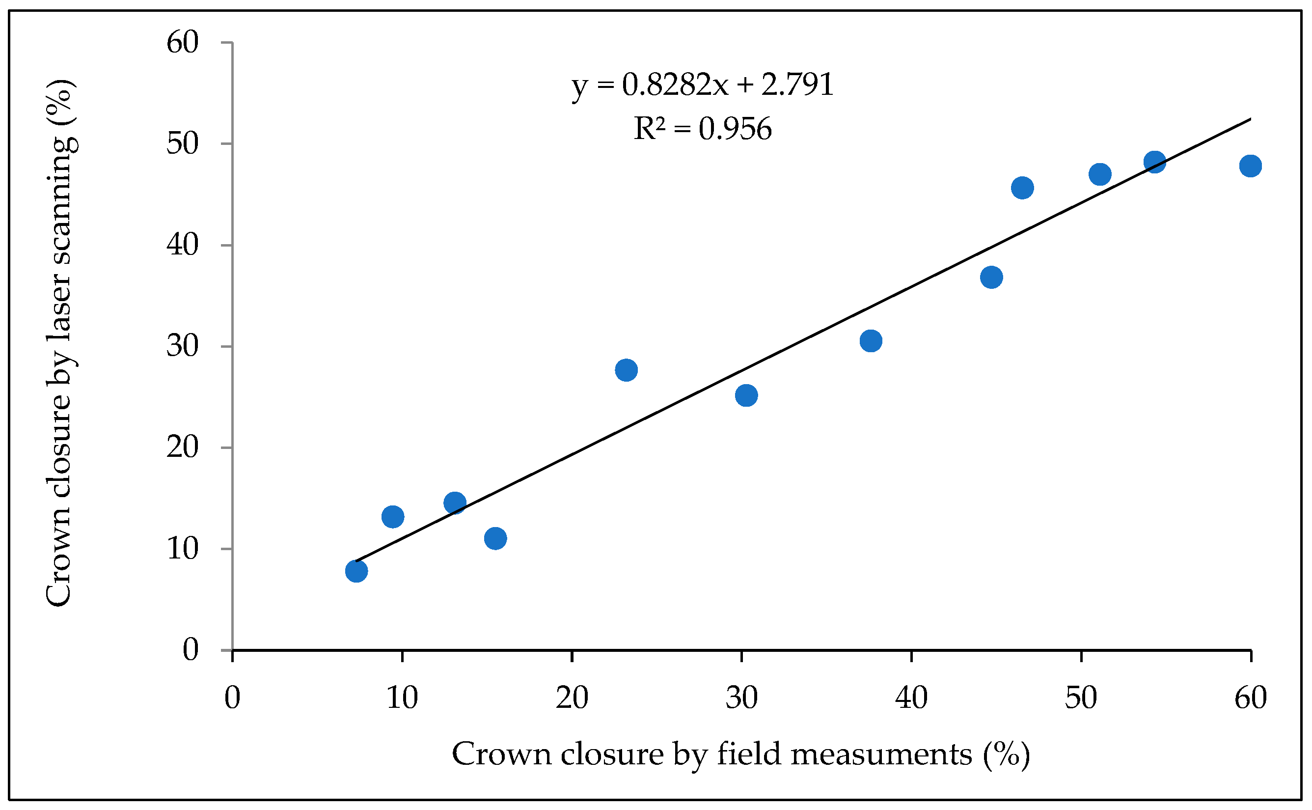
Figure A2.
Statistical characteristics of canopy cover on different elevation levels of transects located on slopes of the Kholodny Belok Ridge (Altai) and Kohosh Ridge (Western Sayan).
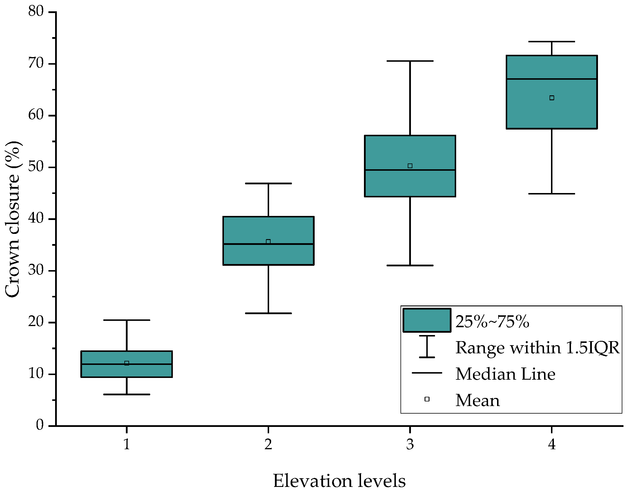
Table A1.
Results of multiple linear regression analysis between tree stand closure on the Kholodny Belok Ridge (Altai) and data from spectral channels of Sentinel-2 images.
Table A2.
Results of multiple linear regression analysis between tree stand closure on the Kohosh (Western Syan) and data from spectral channels of Sentinel-2 images.
Table A3.
Length of treelines estimated using WorldCover and historic topographic maps.
References
- Intergovernmental Panel on Climate Change. Working Group I; WMO; UNEP. Climate Change 2021: The Physical Science Basis Summary for Policymakers. Working Group I Contribution of to the Sixth Assessment Report of the Intergovernmental Panel on Climate Change; Cambridge University Press: Cambridge, UK, 2021; p. 31. [Google Scholar]
- Körner, C. Alpine Treelines: Functional Ecology of the Global High Elevation Tree Limits; Springer: Basel, Switzerland, 2012. [Google Scholar]
- Chan, W.P.; Lenoir, J.; Mai, G.S.; Kuo, H.C.; Chen, I.C.; Shen, S.F. Climate Velocities and Species Tracking in Global Mountain Regions. Nature 2024, 629, 114–120. [Google Scholar] [CrossRef] [Scilit]
- Hansson, A.; Dargusch, P.; Shulmeister, J. A Review of Modern Treeline Migration, the Factors Controlling It and the Implications for Carbon Storage. J. Mt. Sci. 2021, 18, 291–306. [Google Scholar] [CrossRef] [Scilit]
- Harsch, M.A.; Hulme, P.E.; McGlone, M.S.; Duncan, R.P. Are Treelines Advancing? A Global Meta-Analysis of Treeline Response to Climate Warming. Ecol. Lett. 2009, 12, 1040–1049. [Google Scholar] [CrossRef] [Scilit]
- Sjögersten, S.; Wookey, P.A. The Impact of Climate Change on Ecosystem Carbon Dynamics at the Scandinavian Mountain Birch Forest-Tundra Heath Ecotone. AMBIO J. Hum. Environ. 2009, 38, 2–10. [Google Scholar] [CrossRef] [Scilit]
- Wang, G.; Ran, F.; Chang, R.; Yang, Y.; Luo, J.; Jianrong, F. Variations in the Live Biomass and Carbon Pools of Abies Georgei along an Elevation Gradient on the Tibetan Plateau, China. For. Ecol. Manag. 2014, 329, 255–263. [Google Scholar] [CrossRef] [Scilit]
- Grafius, D.R.; Malanson, G.P. Biomass Distributions in Dwarf Tree, Krummholz, and Tundra Vegetation in the Alpine Treeline Ecotone. Phys. Geogr. 2015, 36, 337–352. [Google Scholar] [CrossRef] [Scilit]
- Moiseev, P.A.; Hagedorn, F.; Balakin, D.S.; Bubnov, M.O.; Devi, N.M.; Kukarskih, V.V.; Mazepa, V.S.; Viyukhin, S.O.; Viyukhina, A.A.; Grigoriev, A.A. Stand Biomass at Treeline Ecotone in Russian Subarctic Mountains Is Primarily Related to Species Composition but Its Dynamics Driven by Improvement of Climatic Conditions. Forests 2022, 13, 254. [Google Scholar] [CrossRef] [Scilit]
- Xin, L.; Yu, N.; Gao-qiang, K.; Tia, L. Contrasting Changes in Above- and below-Ground Biomass Allocation across Treeline Ecotones in Southeast Tibet. J. Mt. Sci. 2016, 13, 2036–2045. [Google Scholar] [CrossRef] [Scilit]
- Hagedorn, F.; Dawes, M.A.; Bubnov, M.O.; Devi, N.M.; Grigoriev, A.A.; Mazepa, V.S.; Nagimov, Z.Y.; Shiyatov, S.G.; Moiseev, P.A. Latitudinal Decline in Stand Biomass and Productivity at the Elevational Treeline in the Ural Mountains despite a Common Thermal Growth Limit. J. Biogeogr. 2020, 47, 1827–1842. [Google Scholar] [CrossRef] [Scilit]
- Mainali, K.; Shrestha, B.B.; Sharma, R.K.; Adhikari, A.; Gurarie, E.; Singer, M.; Parmesan, C. Contrasting Responses to Climate Change at Himalayan Treelines Revealed by Population Demographics of Two Dominant Species. Ecol. Evol. 2020, 10, 1209–1222. [Google Scholar] [CrossRef] [Scilit]
- Van Bogaert, R.; Haneca, K.; Hoogesteger, J.; Jonasson, C.; De Dapper, M.; Callaghan, T.V. A Century of Tree Line Changes in Sub-Arctic Sweden Shows Local and Regional Variability and Only a Minor Influence of 20th Century Climate Warming. J. Biogeogr. 2011, 38, 907–921. [Google Scholar] [CrossRef] [Scilit]
- Hagedorn, F.; Shiyatov, S.G.; Mazepa, V.S.; Devi, N.M.; Grigor’ev, A.A.; Bartysh, A.A.; Fomin, V.V.; Kapralov, D.S.; Terent’ev, M.; Bugman, H.; et al. Treeline Advances along the Ural Mountain Range—Driven by Improved Winter Conditions? Glob. Change Biol. 2014, 20, 3530–3543. [Google Scholar] [CrossRef] [Scilit]
- Moiseev, P.A.; Bubnov, M.O.; Devi, N.M.; Nagimov, Z.Y. Changes in the Structure and Phytomass of Tree Stands at the Upper Limit of Their Growth in the Southern Urals. Russ. J. Ecol. 2016, 47, 219–227. [Google Scholar] [CrossRef] [Scilit]
- Hofgaard, A.; Tømmervik, H.; Rees, G.; Hanssen, F. Latitudinal Forest Advance in Northernmost Norway since the Early 20th Century. J. Biogeogr. 2013, 40, 938–949. [Google Scholar] [CrossRef] [Scilit]
- Rannow, S. Do Shifting Forest Limits in South-West Norway Keep up with Climate Change? Scand. J. For. Res. 2013, 28, 574–580. [Google Scholar] [CrossRef] [Scilit]
- Garbarino, M.; Morresi, D.; Anselmetto, N.; Weisberg, P.J. Treeline Remote Sensing: From Tracking Treeline Shifts to Multi-Dimensional Monitoring of Ecotonal Change. Remote Sens. Ecol. Conserv. 2023, 9, 729–742. [Google Scholar] [CrossRef] [Scilit]
- Räsänen, A.; Juutinen, S.; Aurela, M.; Virtanen, T. Predicting Aboveground Biomass in Arctic Landscapes Using Very High Spatial Resolution Satellite Imagery and Field Sampling. Int. J. Remote Sens. 2019, 40, 1175–1199. [Google Scholar] [CrossRef] [Scilit]
- Bratsch, S.; Epstein, H.; Buchhorn, M.; Walker, D.; Landes, H. Relationships between Hyperspectral Data and Components of Vegetation Biomass in Low Arctic Tundra Communities at Ivotuk, Alaska. Environ. Res. Lett. 2017, 12, 025003. [Google Scholar] [CrossRef] [Scilit]
- Epstein, H.E.; Raynolds, M.K.; Walker, D.A.; Bhatt, U.S.; Tucker, C.J.; Pinzon, J.E. Dynamics of Aboveground Phytomass of the Circumpolar Arctic Tundra during the Past Three Decades. Environ. Res. Lett. 2012, 7, 015506. [Google Scholar] [CrossRef] [Scilit]
- Berner, L.T.; Jantz, P.; Tape, K.D.; Goetz, S.J. Tundra Plant Above-Ground Biomass and Shrub Dominance Mapped across the North Slope of Alaska. Environ. Res. Lett. 2018, 13, 035002. [Google Scholar] [CrossRef] [Scilit]
- Berner, L.T.; Beck, P.S.A.; Loranty, M.M.; Alexander, H.D.; MacK, M.C.; Goetz, S.J. Cajander Larch (Larix cajanderi) Biomass Distribution, Fire Regime and Post-Fire Recovery in Northeastern Siberia. Biogeosciences 2012, 9, 3943–3959. [Google Scholar] [CrossRef] [Scilit]
- Shevtsova, I.; Heim, B.; Kruse, S.; Schröder, J.; Troeva, E.I.; Pestryakova, L.A.; Zakharov, E.S.; Herzschuh, U. Strong Shrub Expansion in Tundra-Taiga, Tree Infilling in Taiga and Stable Tundra in Central Chukotka (North-Eastern Siberia) between 2000 and 2017. Environ. Res. Lett. 2020, 15, 085006. [Google Scholar] [CrossRef] [Scilit]
- Shevtsova, I.; Herzschuh, U.; Heim, B.; Schulte, L.; Stünzi, S.; Pestryakova, L.; Zakharov, E.; Kruse, S. Recent Above-Ground Biomass Changes in Central Chukotka (Russian Far East) Using Field Sampling and Landsat Satellite Data. Biogeosciences 2021, 18, 3343–3366. [Google Scholar] [CrossRef] [Scilit]
- Bennett, L.; Yu, Z.; Wasowski, R.; Selland, S.; Otway, S.; Boisvert, J. Individual Tree Detection and Classification from RGB Satellite Imagery with Applications to Wildfire Fuel Mapping and Exposure Assessments. Int. J. Wildl. Fire 2024, 33, WF24008. [Google Scholar] [CrossRef] [Scilit]
- Morley, P.J.; Donoghue, D.N.M.; Chen, J.C.; Jump, A.S. Integrating Remote Sensing and Demography for More Efficient and Effective Assessment of Changing Mountain Forest Distribution. Ecol. Inform. 2018, 43, 106–115. [Google Scholar] [CrossRef] [Scilit]
- Ranson, K.J.; Montesano, P.M.; Nelson, R. Object-Based Mapping of the Circumpolar Taiga-Tundra Ecotone with MODIS Tree Cover. Remote Sens. Environ. 2011, 115, 3670–3680. [Google Scholar] [CrossRef] [Scilit]
- Nizametdinov, N.F.; Shalaumova, Y.V.; Mazepa, V.S.; Moiseev, P.A. Assessment of Past Decadal Dynamics of Tree Stands in Forest–Tundra Transition Zone on the Polar Ural Mountains Calibrated Using Historical and Modern Field Measurements. Forests 2022, 13, 2107. [Google Scholar] [CrossRef] [Scilit]
- Brieger, F.; Herzschuh, U.; Pestryakova, L.A.; Bookhagen, B.; Zakharov, E.S.; Kruse, S. Advances in the Derivation of Northeast Siberian Forest Metrics Using High-Resolution UAV-Based Photogrammetric Point Clouds. Remote Sens. 2019, 11, 1447. [Google Scholar] [CrossRef] [Scilit]
- Mienna, I.M.; Klanderud, K.; Ørka, H.O.; Bryn, A.; Bollandsås, O.M. Land Cover Classification of Treeline Ecotones along a 1100 Km Latitudinal Transect Using Spectral- and Three-Dimensional Information from UAV-Based Aerial Imagery. Remote Sens. Ecol. Conserv. 2022, 8, 536–550. [Google Scholar] [CrossRef] [Scilit]
- Fromm, M.; Schubert, M.; Castilla, G.; Linke, J.; McDermid, G. Automated Detection of Conifer Seedlings in Drone Imagery Using Convolutional Neural Networks. Remote Sens. 2019, 11, 2585. [Google Scholar] [CrossRef] [Scilit]
- Brede, B.; Terryn, L.; Barbier, N.; Bartholomeus, H.M.; Bartolo, R.; Calders, K.; Derroire, G.; Krishna Moorthy, S.M.; Lau, A.; Levick, S.R.; et al. Non-Destructive Estimation of Individual Tree Biomass: Allometric Models, Terrestrial and UAV Laser Scanning. Remote Sens. Environ. 2022, 280, 113180. [Google Scholar] [CrossRef] [Scilit]
- Nasiri, V.; Darvishsefat, A.A.; Arefi, H.; Pierrot-Deseilligny, M.; Namiranian, M.; Le Bris, A. Unmanned Aerial Vehicles (Uav)-Based Canopy Height Modeling under Leaf-on and Leaf-off Conditions for Determining Tree Height and Crown Diameter (Case Study: Hyrcanian Mixed Forest). Can. J. For. Res. 2021, 51, 962–971. [Google Scholar] [CrossRef] [Scilit]
- Panagiotidis, D.; Abdollahnejad, A.; Surový, P.; Chiteculo, V. Determining Tree Height and Crown Diameter from High-Resolution UAV Imagery. Int. J. Remote Sens. 2017, 38, 2392–2410. [Google Scholar] [CrossRef] [Scilit]
- Shimizu, K.; Nishizono, T.; Kitahara, F.; Fukumoto, K.; Saito, H. Integrating Terrestrial Laser Scanning and Unmanned Aerial Vehicle Photogrammetry to Estimate Individual Tree Attributes in Managed Coniferous Forests in Japan. Int. J. Appl. Earth Obs. Geoinf. 2022, 106, 102658. [Google Scholar] [CrossRef] [Scilit]
- Lisein, J.; Pierrot-Deseilligny, M.; Bonnet, S.; Lejeune, P. A Photogrammetric Workflow for the Creation of a Forest Canopy Height Model from Small Unmanned Aerial System Imagery. Forests 2013, 4, 922–944. [Google Scholar] [CrossRef] [Scilit]
- Maguire, A.J.; Eitel, J.U.H.; Vierling, L.A.; Johnson, D.M.; Griffin, K.L.; Boelman, N.T.; Jensen, J.E.; Greaves, H.E.; Meddens, A.J.H. Terrestrial Lidar Scanning Reveals Fine-Scale Linkages between Microstructure and Photosynthetic Functioning of Small-Stature Spruce Trees at the Forest-Tundra Ecotone. Agric. For. Meteorol. 2019, 269–270, 157–168. [Google Scholar] [CrossRef] [Scilit]
- Noordermeer, L.; Bielza, J.C.; Saarela, S.; Gobakken, T.; Bollandsås, O.M.; Næsset, E. Monitoring Tree Occupancy and Height in the Norwegian Alpine Treeline Using a Time Series of Airborne Laser Scanner Data. Int. J. Appl. Earth Obs. Geoinf. 2023, 117, 103201. [Google Scholar] [CrossRef] [Scilit]
- Liang, X.; Kukko, A.; Hyyppä, J.; Lehtomäki, M.; Pyörälä, J.; Yu, X.; Kaartinen, H.; Jaakkola, A.; Wang, Y. In-Situ Measurements from Mobile Platforms: An Emerging Approach to Address the Old Challenges Associated with Forest Inventories. ISPRS J. Photogramm. Remote Sens. 2018, 143, 97–107. [Google Scholar] [CrossRef] [Scilit]
- Nyström, M.; Holmgren, J.; Olsson, H. Prediction of Tree Biomass in the Forest-Tundra Ecotone Using Airborne Laser Scanning. Remote Sens. Environ. 2012, 123, 271–279. [Google Scholar] [CrossRef] [Scilit]
- Mukhopadhyay, R.; Næsset, E.; Gobakken, T.; Mienna, I.M.; Bielza, J.C.; Austrheim, G.; Persson, H.J.; Ørka, H.O.; Roald, B.E.; Bollandsås, O.M. Mapping and Estimating Aboveground Biomass in an Alpine Treeline Ecotone under Model-Based Inference. Remote Sens. 2023, 15, 3508. [Google Scholar] [CrossRef] [Scilit]
- Moiseev, P.A.; Nizametdinov, N.F. Climatic Effects on Position and Dynamics of Upper Open Forest Boundary in Altay and Western Sayan in the Last 60 Years. Forests 2023, 14, 1987. [Google Scholar] [CrossRef] [Scilit]
- Myglan, V.S.; Ovchinnikov, D.V.; Vaganov, E.A.; Bykov, N.I.; Gerasimova, O.V.; Sidorova, O.V.; Silkin, P.P. Construction of 1772-Year Tree Ring Width Chronology for Altay Republic. Izv. Akad. Nauk. Seriya Geogr. 2009, 6, 70–77. [Google Scholar]
- Myglan, V.S.; Oidupaa, O.C.; Vaganov, E.A. A 2367-Year Tree-Ring Chronology for the Altai-Sayan Region (Mongun-Taiga Mountain Massif). Archaeol. Ethnol. Anthropol. Eurasia 2012, 40, 76–83. [Google Scholar] [CrossRef] [Scilit]
- Oydupaa, O.C.; Barinov, V.; Serdobov, V.N.; Myglan, V. Reconstruction and Analysis of 1104-Year Tree-Ring Chronology Tarys for Altai-Sayan Region ( Southeastern Tuva ). J. Sib. Fed. Univ. Biol. 2011, 4, 368–377. [Google Scholar]
- Lipka, O.N.; Vertyankina, V.; Korzukhin, M.; Kurganova, I.N. The Third Assessment Report of the Russian Federal Service for Hydrometeorology and Environmental Monitoring on Climate Change and Its Consequences in the Russian Federation; Katzov, V.M., Ed.; Naukoyomkiye Tekhnologiyi Press: Saint Petersburg, Russia, 2022. [Google Scholar]
- Klinge, M.; Böhner, J.; Lehmkuhl, F. Climate Pattern, Snow- and Timberlines in the Altai Mountains, Central Asia. Erdkunde 2003, 57, 296–308. [Google Scholar] [CrossRef] [Scilit]
- Narozhniy, Y.; Zemtsov, V. Current State of the Altai Glaciers (Russia) and Trends over the Period of Instrumental Observations 1952–2008. Ambio 2011, 40, 575–588. [Google Scholar] [CrossRef] [Scilit]
- Nazarov, A.N.; Myglan, V.S. The Possibility of Construction of the 6000-Year Chronology for Siberian Pine in the Central Altai. J. Sib. Fed. Univ. Biol. 2012, 5, 70–88. [Google Scholar] [CrossRef] [Scilit]
- Ovtchinnokov, D.V.; Vaganov, E.A. Dendrochronological Characteristics of Larix Sibirica (Larix sibirica Ldb.) on the Upper Timberline of Wood in Mountain Altai. Contemp. Probl. Ecol. 1999, 2, 145–152. [Google Scholar]
- Kharuk, V.I.; Petrov, I.A.; Im, S.T.; Golyukov, A.S.; Dvinskaya, M.L.; Shushpanov, A.S. Tree Clusters Migration into Alpine Tundra, Siberia. J. Mt. Sci. 2022, 19, 3426–3440. [Google Scholar] [CrossRef] [Scilit]
- Savchuk, D.A.; Timoshok, E.E.; Filimonova, E.O.; Nikolaev, S.A. Dynamics of the Upper Forest Limit on the Katunsky Ridge (Altai Mountains) over the Past 120 Years. Russ. J. Ecol. 2023, 475, 416–421. [Google Scholar] [CrossRef] [Scilit]
- Buslov, M.M.; Geng, H.; Travin, A.V.; Otgonbaatar, D.; Kulikova, A.V.; Ming, C.; Glorie, S.; Semakov, N.N.; Rubanova, E.S.; Abildaeva, M.A.; et al. Tectonics and Geodynamics of Gorny Altai and Adjacent Structures of the Altai-Sayan Folded Area. Geol. Geophys. 2020, 54, 1600–1627. [Google Scholar] [CrossRef] [Scilit]
- Grigoriev, A.; Korkina, I.; Vyukhin, S.; Shalaumova, Y.; Nizametdinov, N.; Balakin, D.; Golikov, D.; Moiseev, P. Forest Ecosystems Response of Woody Vegetation and Soils to Modern Climate Change in the Altai Mountains. For. Ecosyst. 2026, 15, 100434. [Google Scholar] [CrossRef] [Scilit]
- Kovalev, R.B. Soils of the Gorno-Altai Autonomous Region; Nauka: Novosibirsk, Russia, 1973. [Google Scholar]
- Braeker, O.U. Der Alterstrend Bei Jahrringdichten Und Jahrringbreiten von Nadelhölzern Und Sein Ausgleich. Mitteilungen Forstl. Bundes-Vers. Wien 1981, 142, 75–102. [Google Scholar]
- Jennings, S.B.; Brown, N.D.; Sheil, D. Assessing Forest Canopies and Understorey Illumination: Canopy Closure, Canopy Cover and Other Measures. Forestry 1999, 72, 59–73. [Google Scholar] [CrossRef] [Scilit]
- Korhonen, L.; Korhonen, K.T.; Rautiainen, M.; Stenberg, P. Estimation of Forest Canopy Cover: A Comparison of Field Measurement Techniques. Silva Fenn. 2006, 40, 577–588. [Google Scholar] [CrossRef] [Scilit]
- Moran, P.A.P. Notes on Continuous Stochastic Phenomena. Biometrika 1950, 37, 17–23. [Google Scholar] [CrossRef] [Scilit]
- Weinmann, M.; Weidner, U. Land-Cover and Land-Use Classification Based on Multitemporal Sentinel-2 Data. In Proceedings of the IGARSS 2018—2018 IEEE International Geoscience and Remote Sensing Symposium, Valencia, Spain, 22–27 July 2018; pp. 4946–4949. [Google Scholar] [CrossRef] [Scilit]
- Arfa, A.; Minaei, M. Utilizing Multitemporal Indices and Spectral Bands of Sentinel-2 to Enhance Land Use and Land Cover Classification with Random Forest and Support Vector Machine. Adv. Space Res. 2024, 74, 5580–5590. [Google Scholar] [CrossRef] [Scilit]
- Ruiz, L.A.; Hermosilla, T.; Mauro, F.; Godino, M. Analysis of the Influence of Plot Size and LiDAR Density on Forest Structure Attribute Estimates. Forests 2014, 5, 936–951. [Google Scholar] [CrossRef] [Scilit]
- Richardson, J.J.; Moskal, L.M. Strengths and Limitations of Assessing Forest Density and Spatial Configuration with Aerial LiDAR. Remote Sens. Environ. 2011, 115, 2640–2651. [Google Scholar] [CrossRef] [Scilit]
- Gorelick, N.; Hancher, M.; Dixon, M.; Ilyushchenko, S.; Thau, D.; Moore, R. Google Earth Engine: Planetary-Scale Geospatial Analysis for Everyone. Remote Sens. Environ. 2017, 202, 18–27. [Google Scholar] [CrossRef] [Scilit]
- Conrad, O.; Bechtel, B.; Bock, M.; Dietrich, H.; Fischer, E.; Gerlitz, L.; Wehberg, J.; Wichmann, V.; Böhner, J. System for Automated Geoscientific Analyses (SAGA) v. 2.1.4. Geosci. Model Dev. 2015, 8, 1991–2007. [Google Scholar] [CrossRef] [Scilit]
- Robertus, Y.V.; Kivatskay, A.V.; Lyubimov, R.V. New Data on the Carbon Balance of the Territory of the Altai Republic. Izv. Akad. Nauk. Seriya Geogr. 2014, 6, 110–113. [Google Scholar] [CrossRef] [Scilit]
- Holtmeier, F.K.; Broll, G. Wind as an Ecological Agent at Treelines in North America, the Alps, and the European Subarctic. Phys. Geogr. 2010, 31, 203–233. [Google Scholar] [CrossRef] [Scilit]
- Rossi, S.; Deslauriers, A.; Anfodillo, T.; Carraro, V. Evidence of Threshold Temperatures for Xylogenesis in Conifers at High Altitudes. Oecologia 2007, 152, 1–12. [Google Scholar] [CrossRef] [Scilit]
- Måren, I.E.; Karki, S.; Prajapati, C.; Yadav, R.K.; Shrestha, B.B. Facing North or South: Does Slope Aspect Impact Forest Stand Characteristics and Soil Properties in a Semiarid Trans-Himalayan Valley? J. Arid Environ. 2015, 121, 112–123. [Google Scholar] [CrossRef] [Scilit]
- Dearborn, K.D.; Danby, R.K. Aspect and Slope Influence Plant Community Composition More than Elevation across Forest-Tundra Ecotones in Subarctic Canada. J. Veg. Sci. 2017, 28, 595–604. [Google Scholar] [CrossRef] [Scilit]
- Sturm, M.; Schimel, J.; Michaelson, G.; Welker, J.M.J.M.; Oberbauer, S.F.S.F.; Liston, G.E.G.E.; Fahnestock, J.; Romanovsky, V.E.V.E. Winter Biological Processes Could Help Convert Arctic Tundra to Shrubland. Bioscience 2005, 55, 17. [Google Scholar] [CrossRef] [Scilit]
- Vitasse, Y.; Hoch, G.; Randin, C.F.; Lenz, A.; Kollas, C.; Körner, C. Tree Recruitment of European Tree Species at Their Current Upper Elevational Limits in the Swiss Alps. J. Biogeogr. 2012, 39, 1439–1449. [Google Scholar] [CrossRef] [Scilit]
- Kuyek, N.J.; Thomas, S.C. Trees Are Larger on South Slopes in Late-Seral Conifer Stands in Northwestern British Columbia. Can. J. For. Res. 2019, 49, 1349–1356. [Google Scholar] [CrossRef] [Scilit]
- Danby, R.K.; Hik, D.S. Variability, Contingency and Rapid Change in Recent Subarctic Alpine Tree Line Dynamics. J. Ecol. 2007, 95, 352–363. [Google Scholar] [CrossRef] [Scilit]
- Zheng, L.; Shi, P.; Zhou, T.; Hou, G.; Song, M.; Yu, F. Tree Regeneration Patterns on Contrasting Slopes at Treeline Ecotones in Eastern Tibet. Forests 2021, 12, 1605. [Google Scholar] [CrossRef] [Scilit]
- Germino, M.J.; Smith, W.K.; Resor, A.C. Conifer Seedling Distribution and Survival in an Alpine-Treeline Ecotone. Plant Ecol. 2002, 162, 157–168. [Google Scholar] [CrossRef] [Scilit]
- Lett, S.; Dorrepaal, E. Global Drivers of Tree Seedling Establishment at Alpine Treelines in a Changing Climate. Funct. Ecol. 2018, 32, 1666–1680. [Google Scholar] [CrossRef] [Scilit]
- Loranger, H.; Zotz, G.; Bader, M.Y. Competitor or Facilitator? The Ambiguous Role of Alpine Grassland for the Early Establishment of Tree Seedlings at Treeline. Oikos 2017, 126, 1625–1636. [Google Scholar] [CrossRef] [Scilit]
- Devi, N.M.; Kukarskih, V.V.; Galimova, A.A.; Mazepa, V.S.; Grigoriev, A.A. Climate Change Evidence in Tree Growth and Stand Productivity at the Upper Treeline Ecotone in the Polar Ural Mountains. For. Ecosyst. 2020, 7, 7. [Google Scholar] [CrossRef] [Scilit]
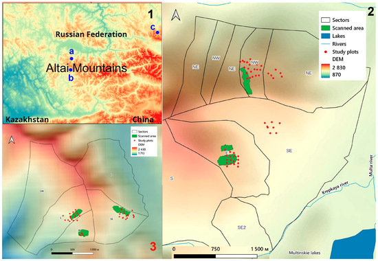
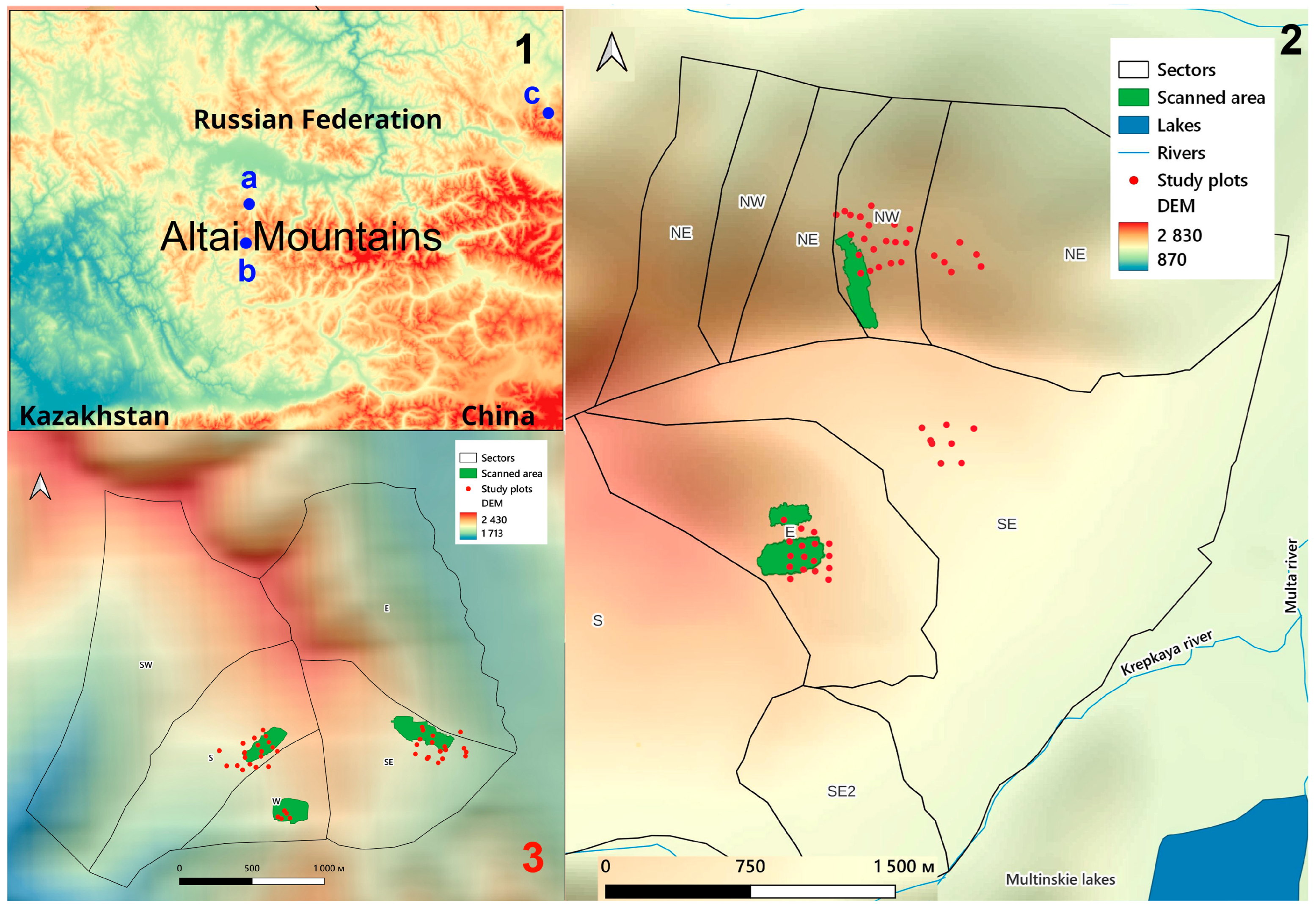
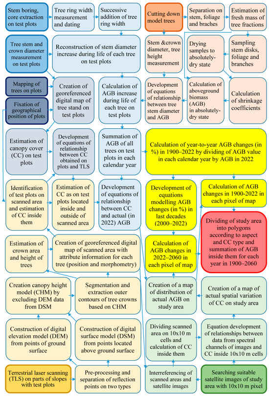
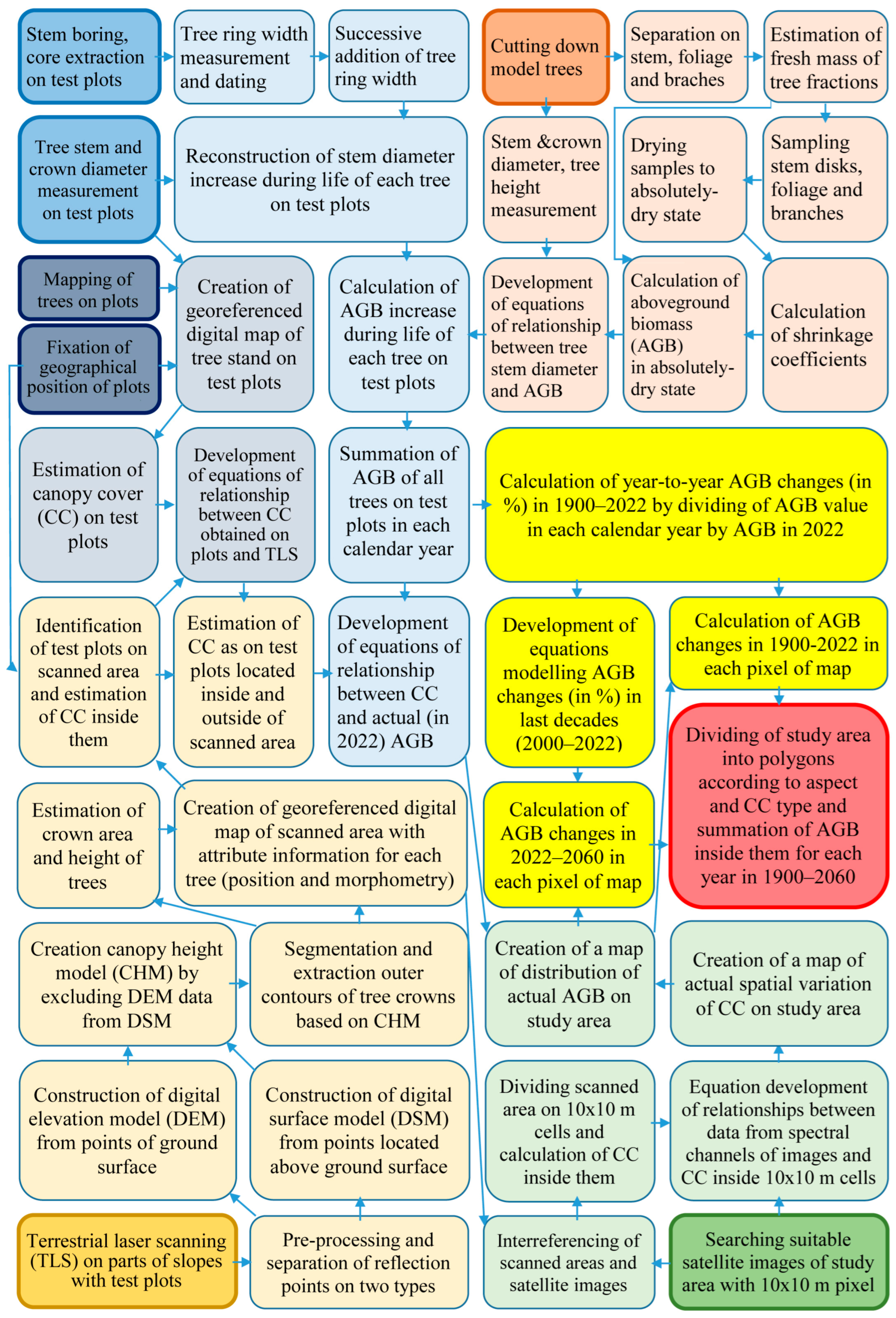
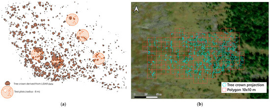
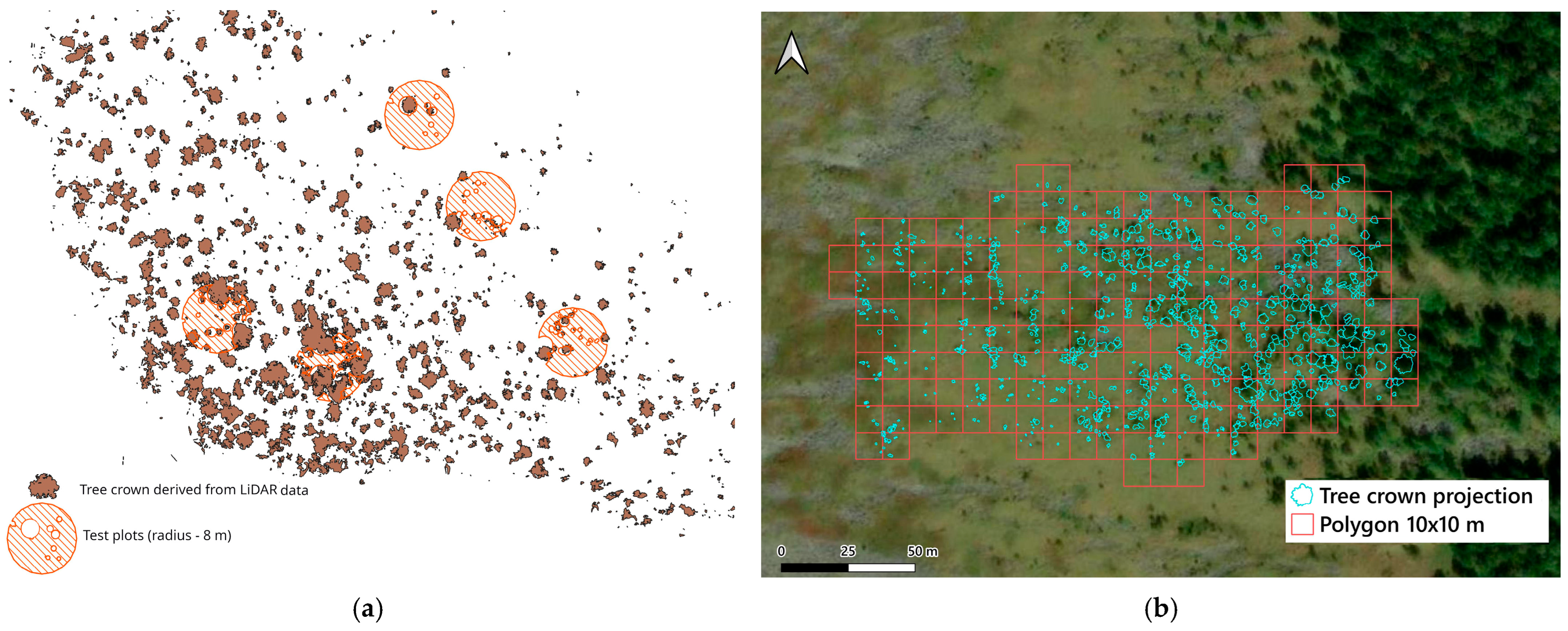
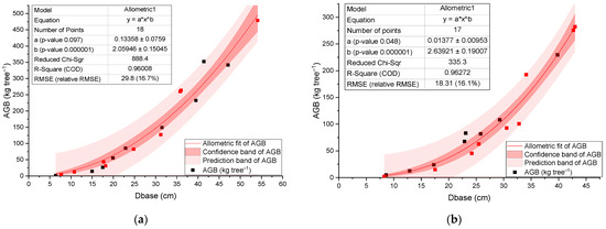
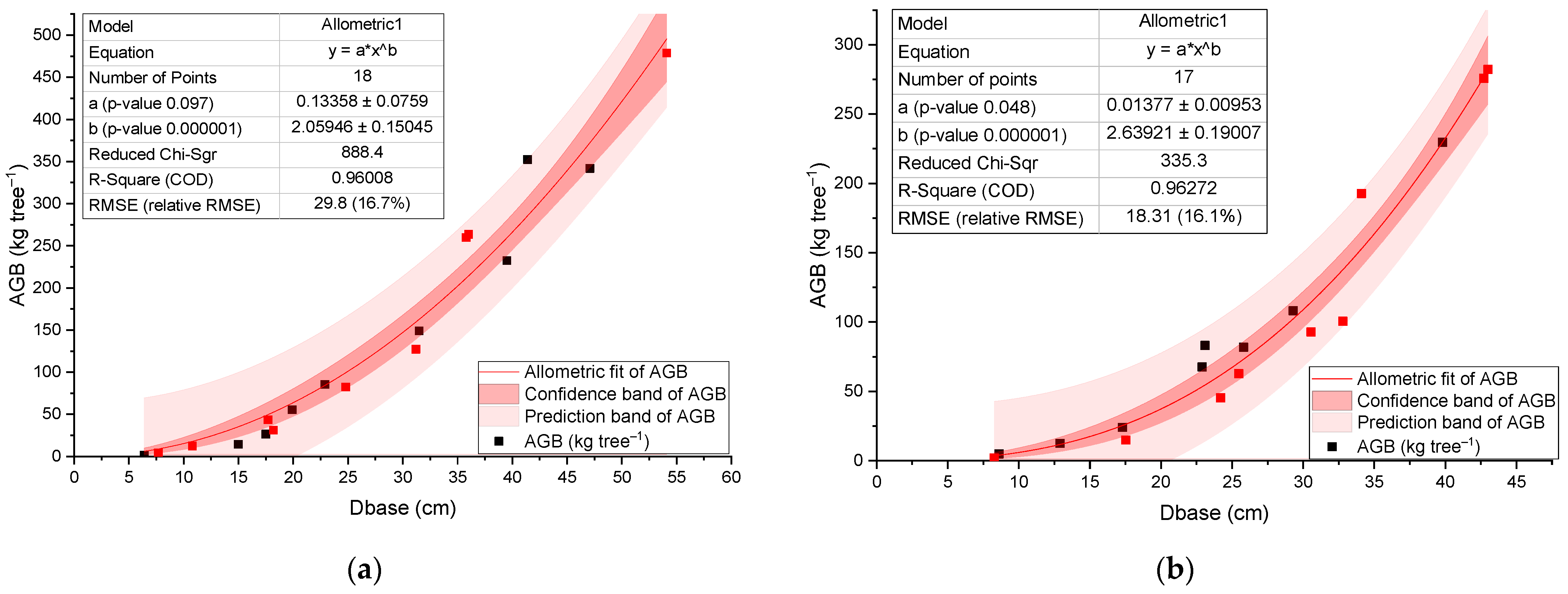
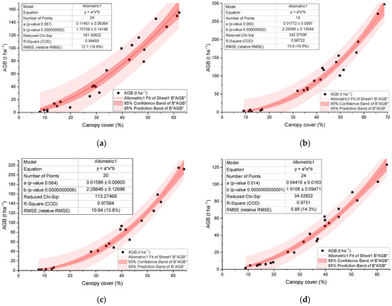
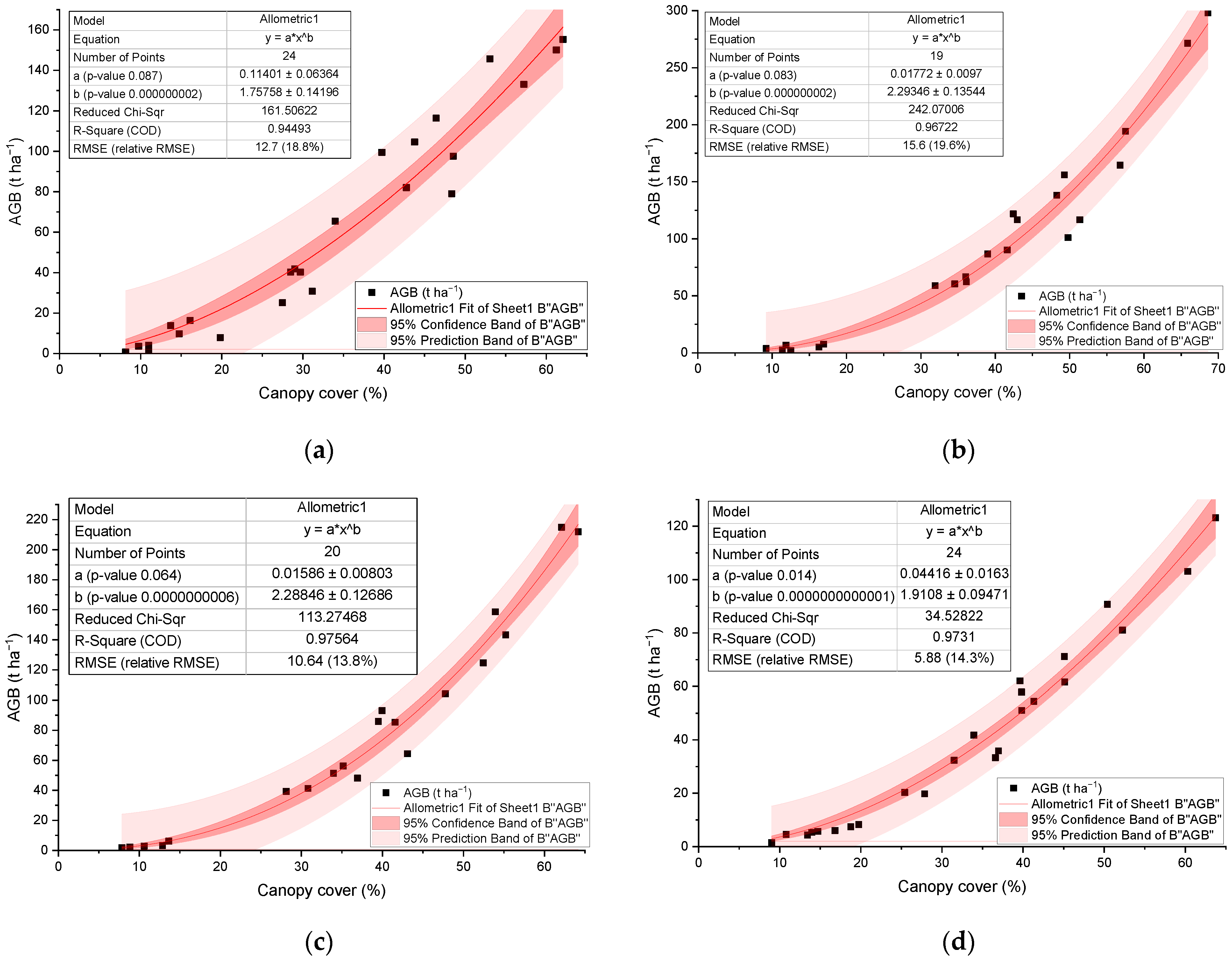
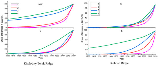
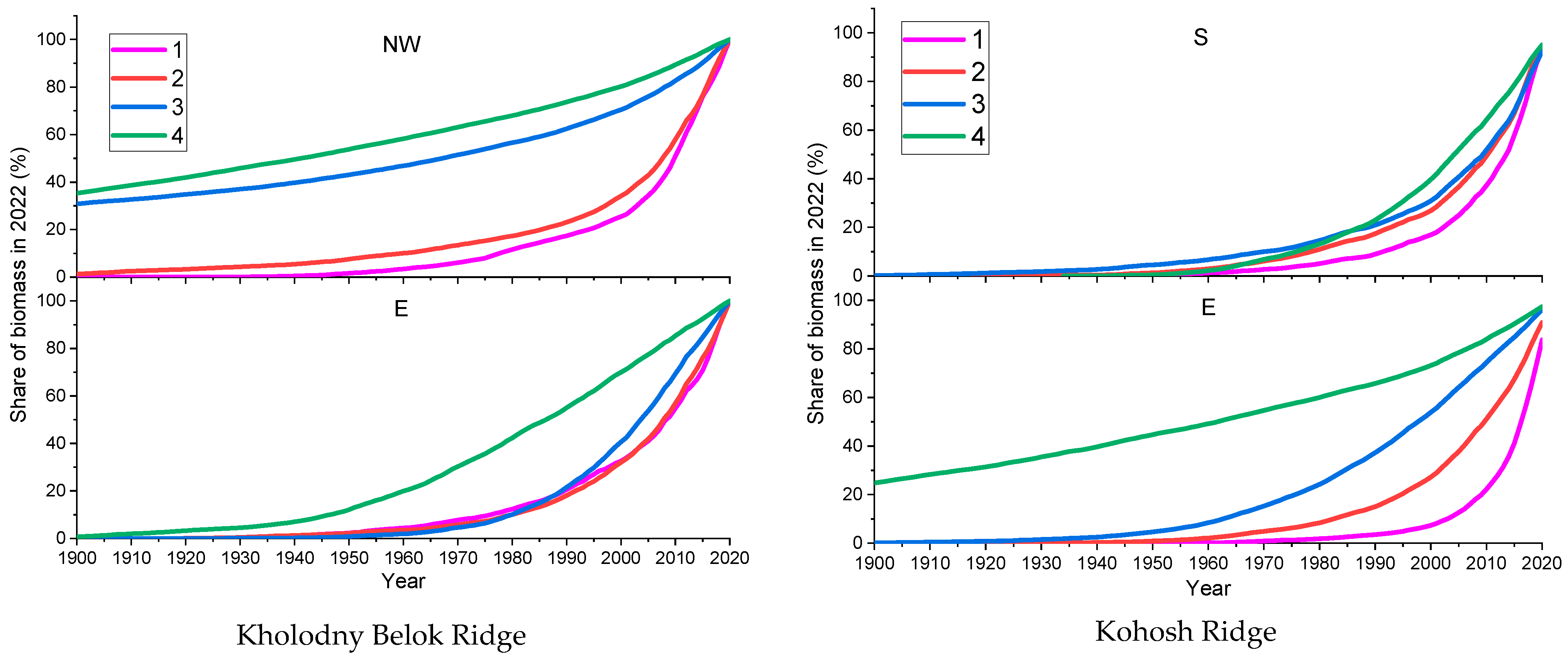
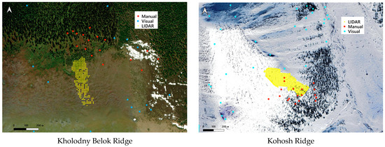
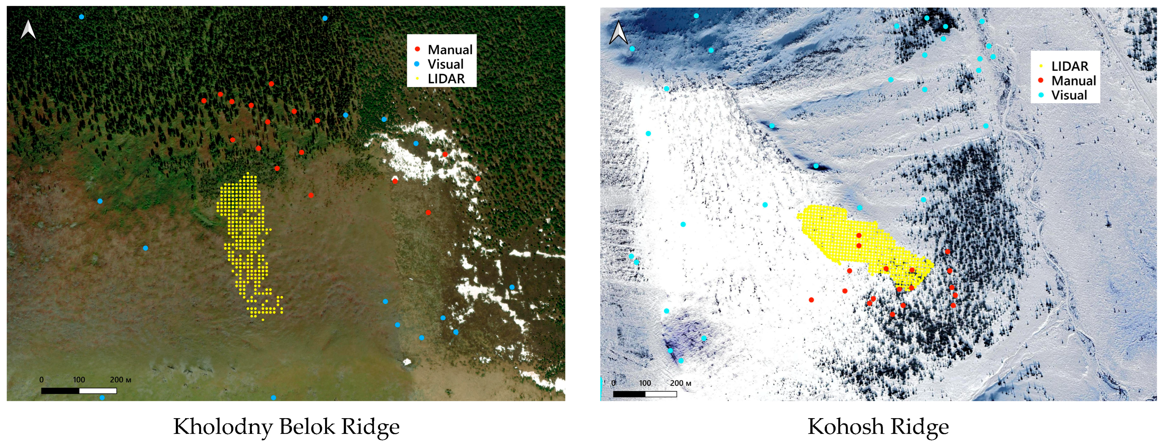
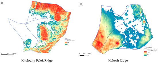
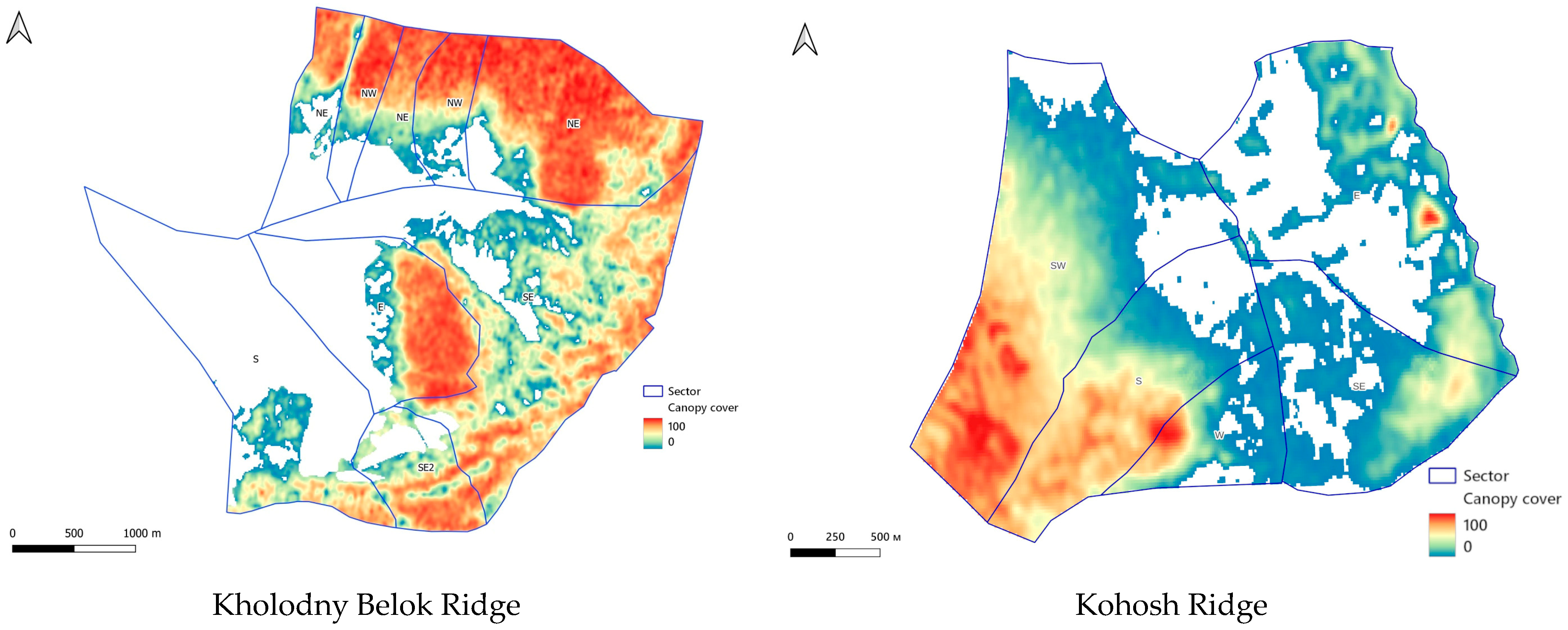
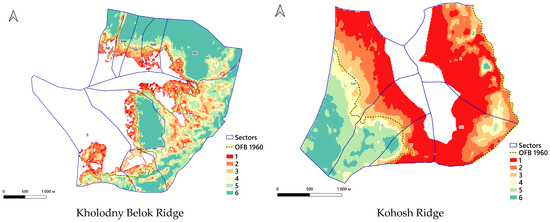
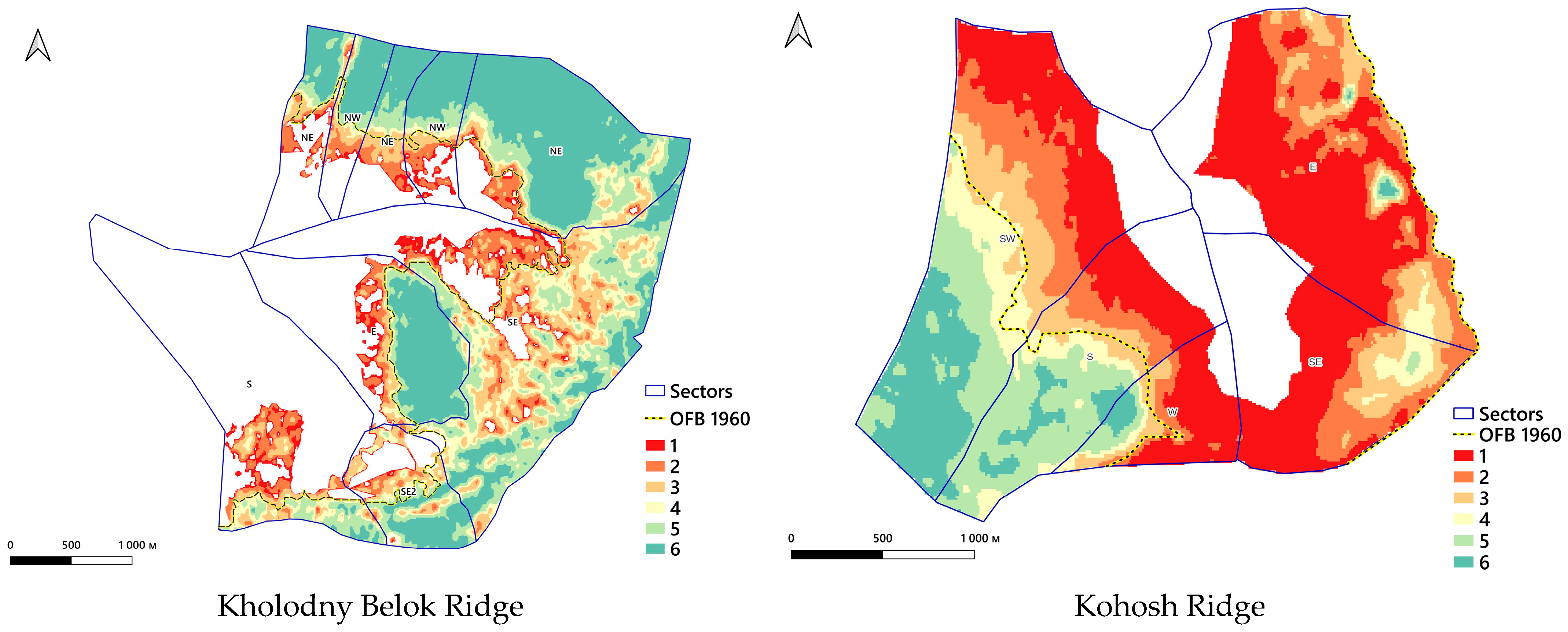
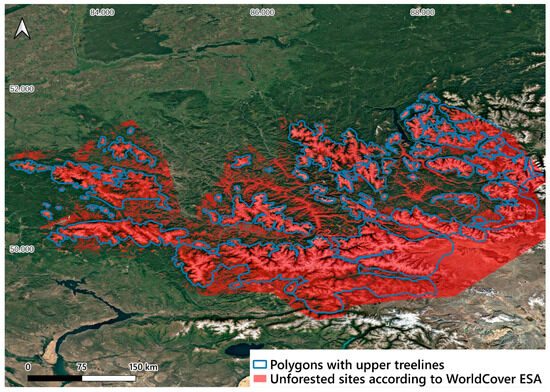
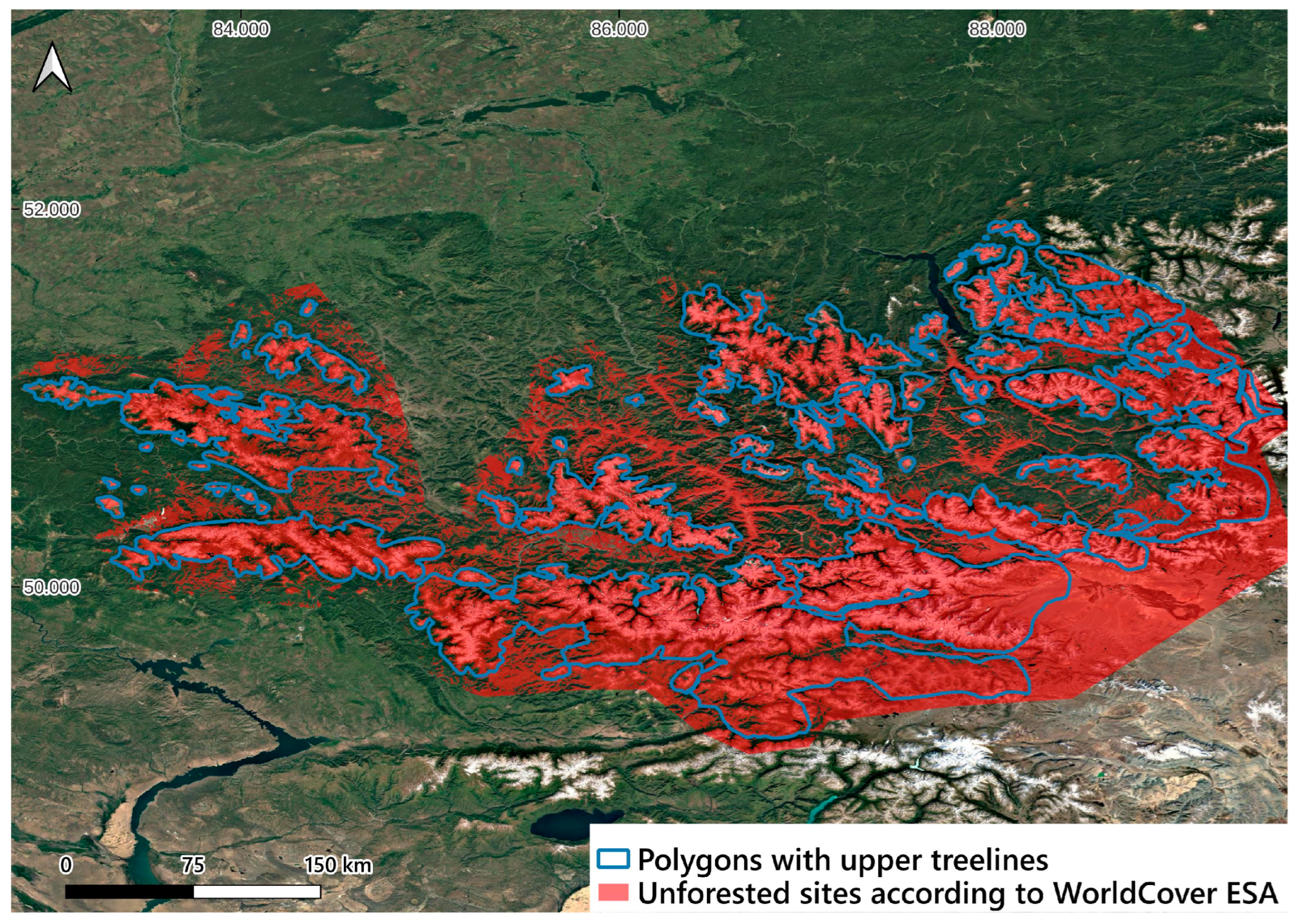
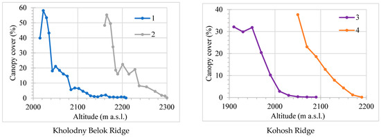
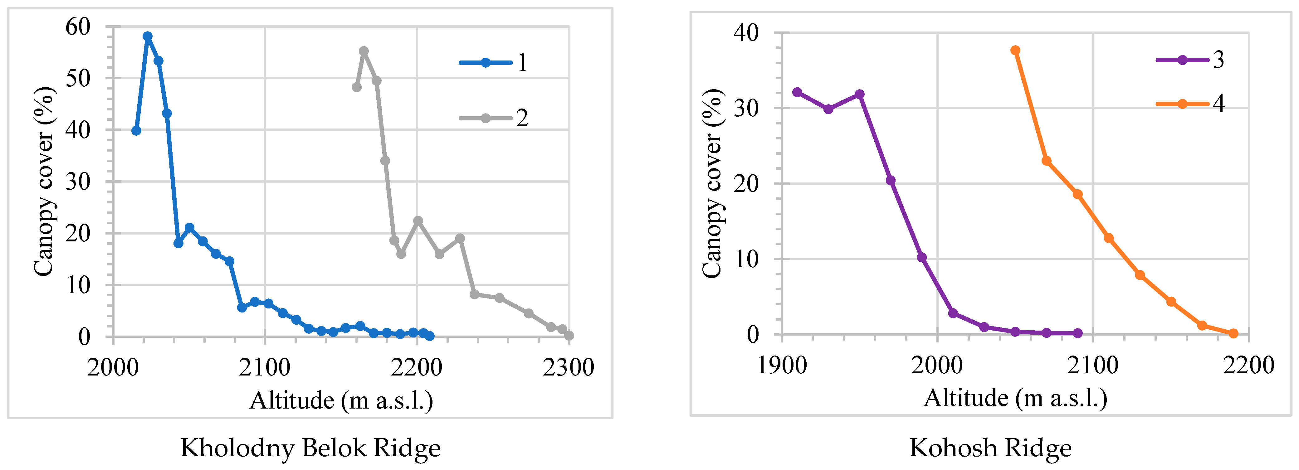
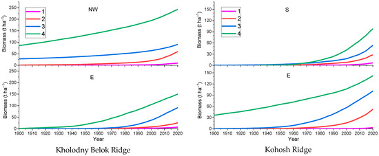
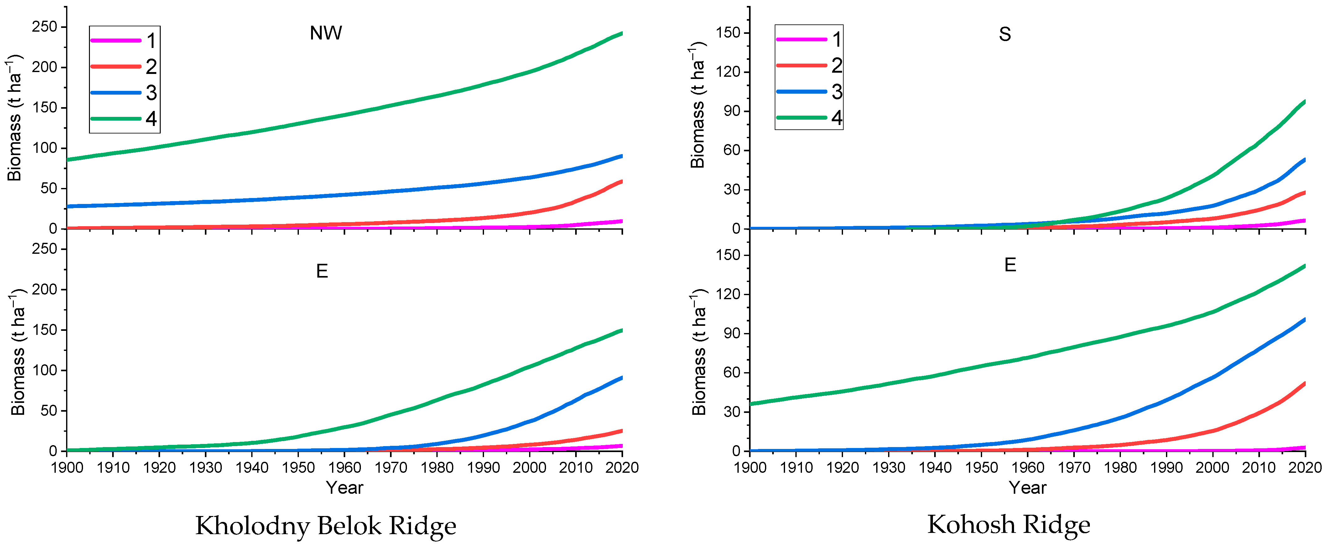
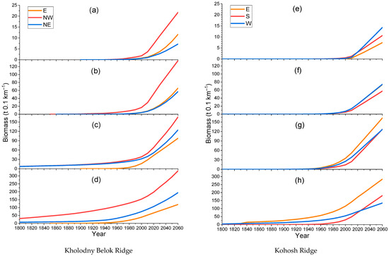
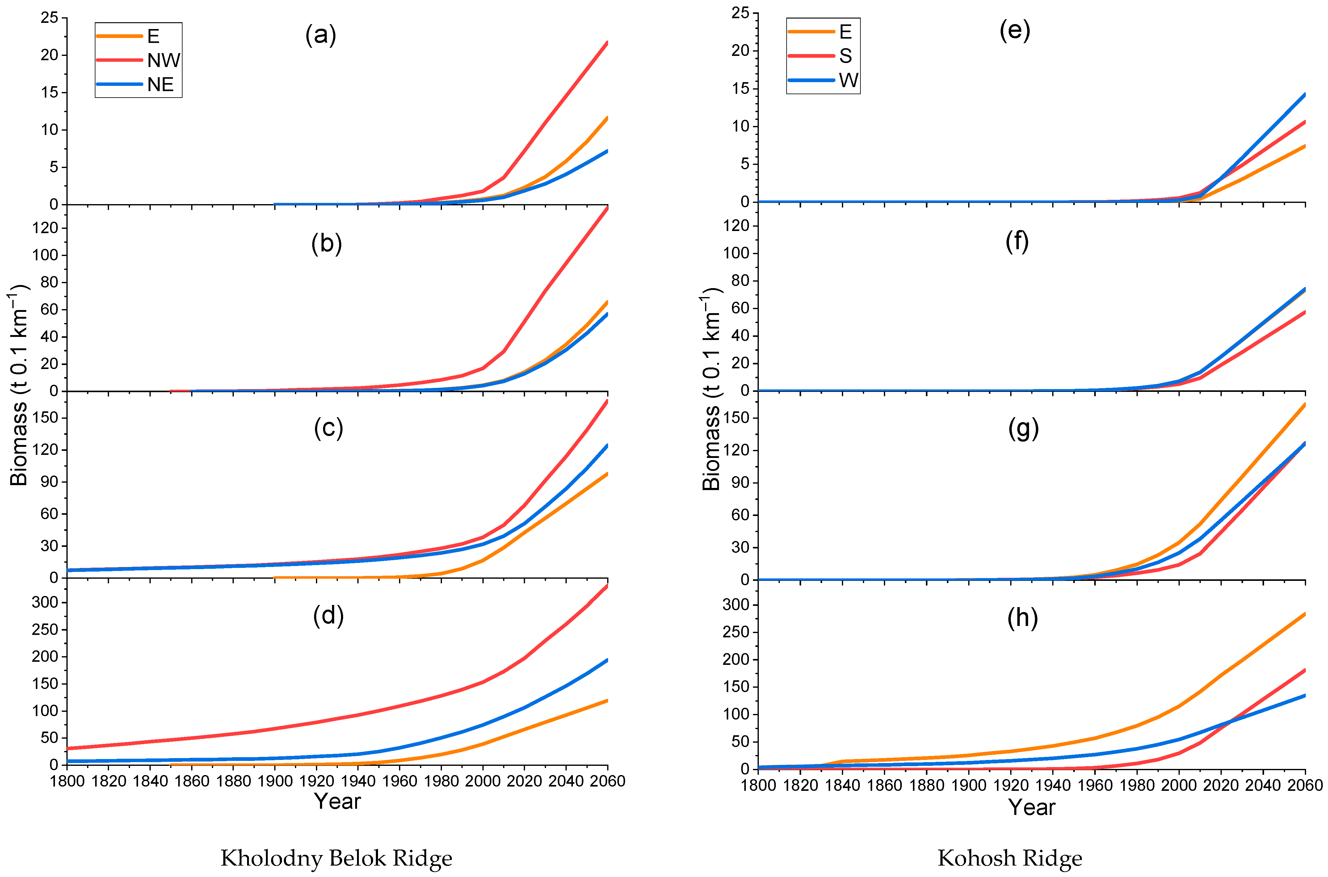
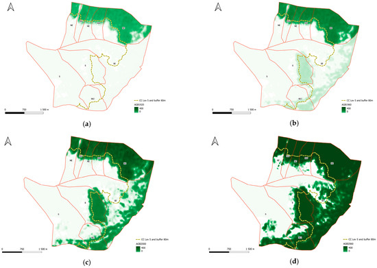
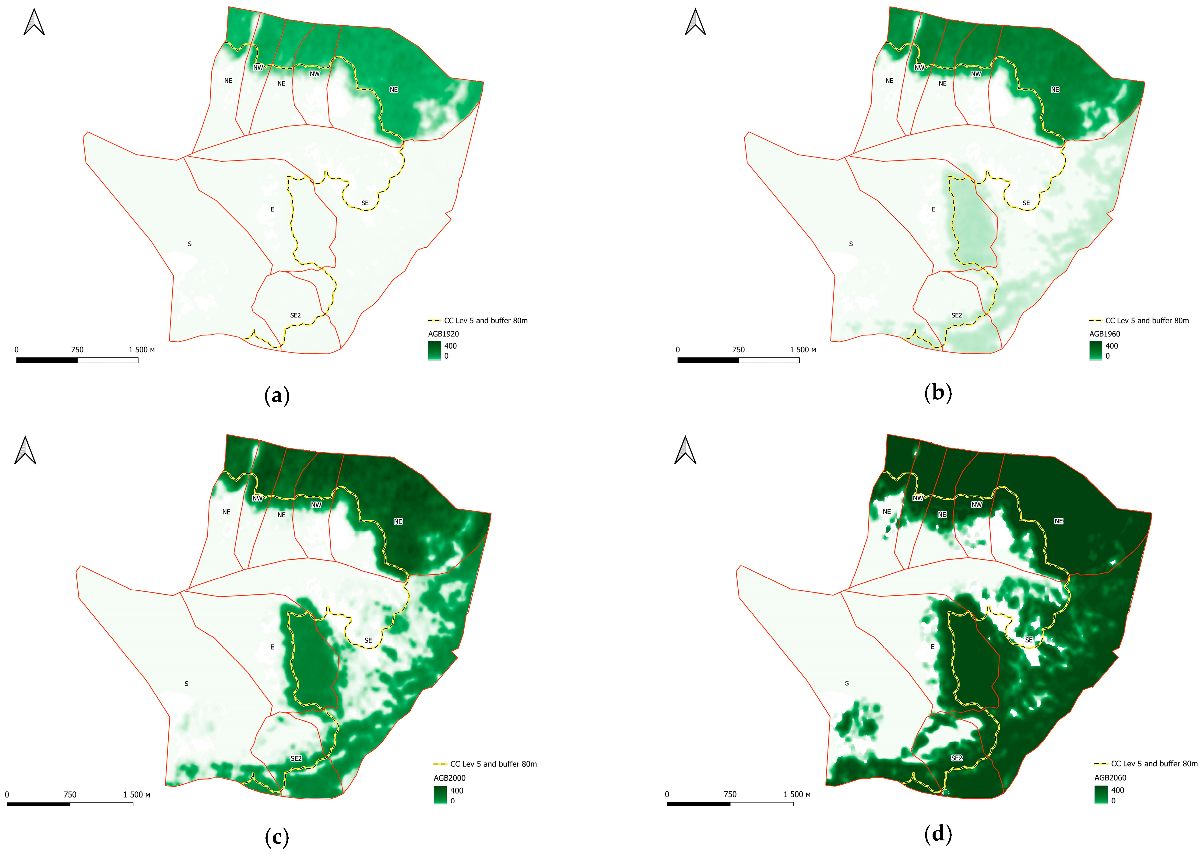
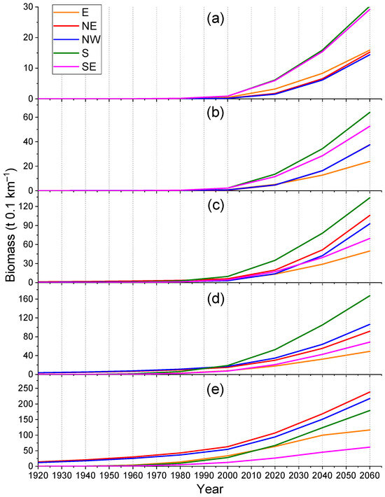
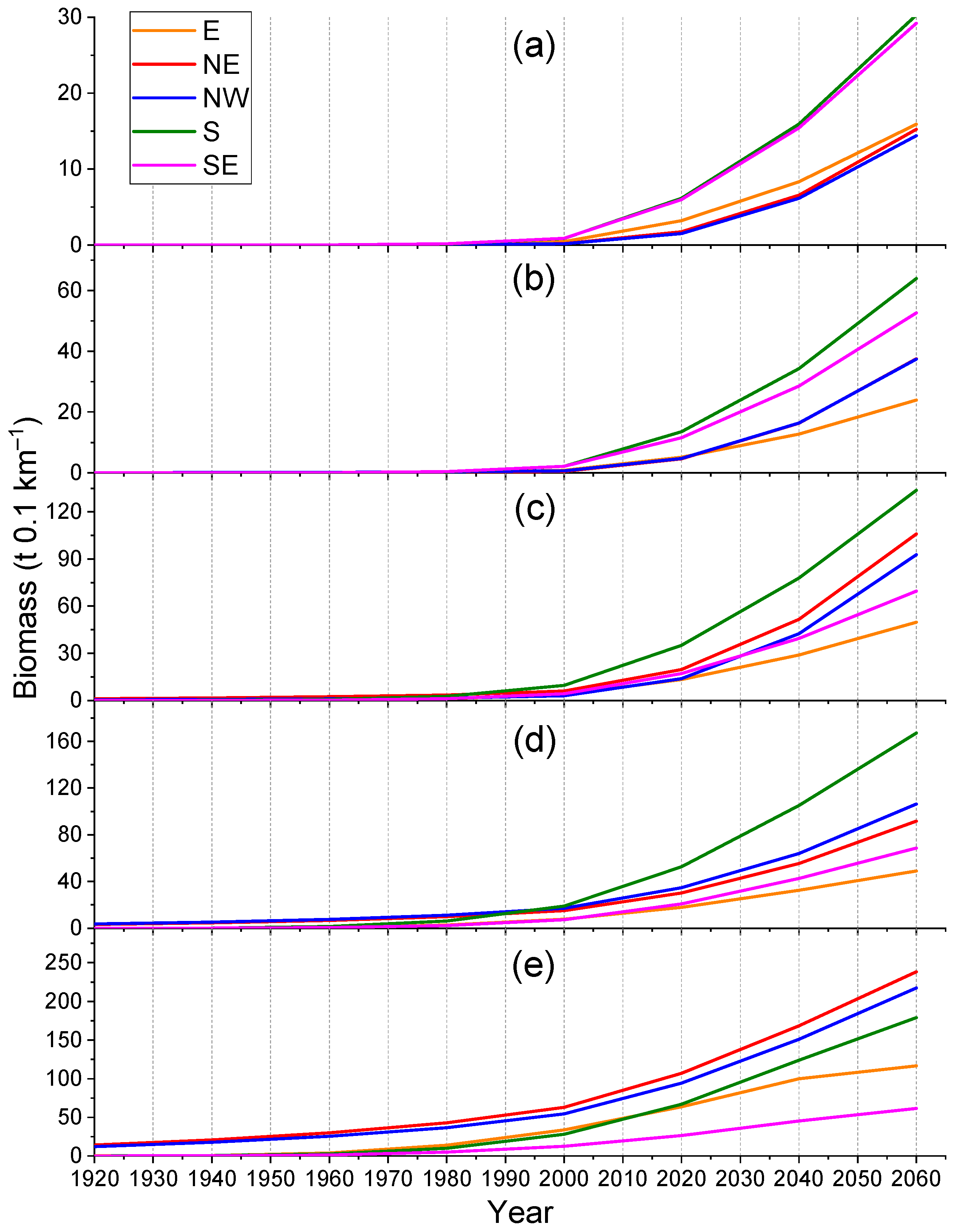
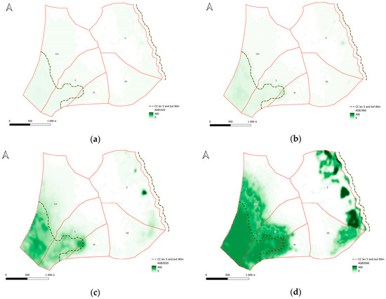
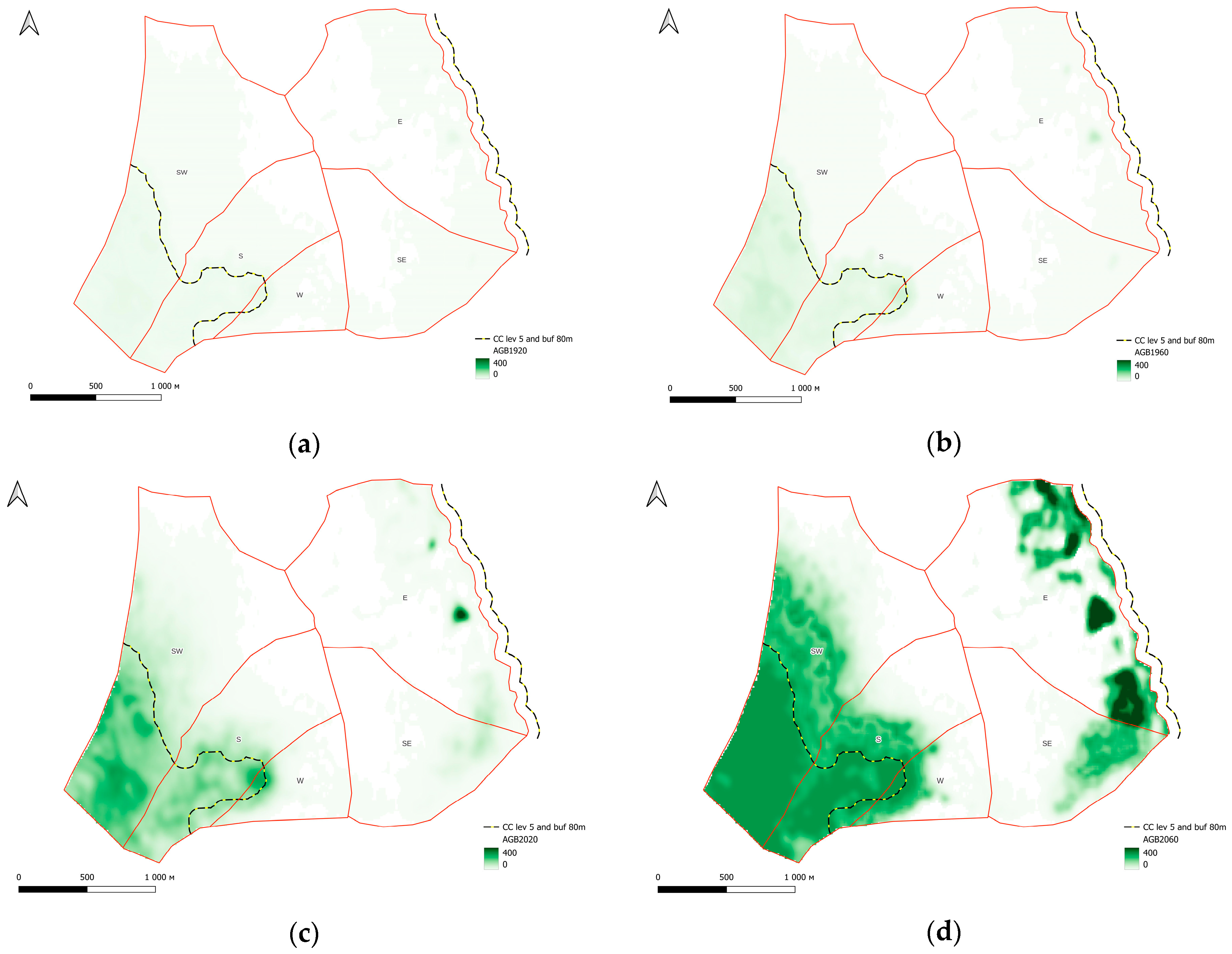
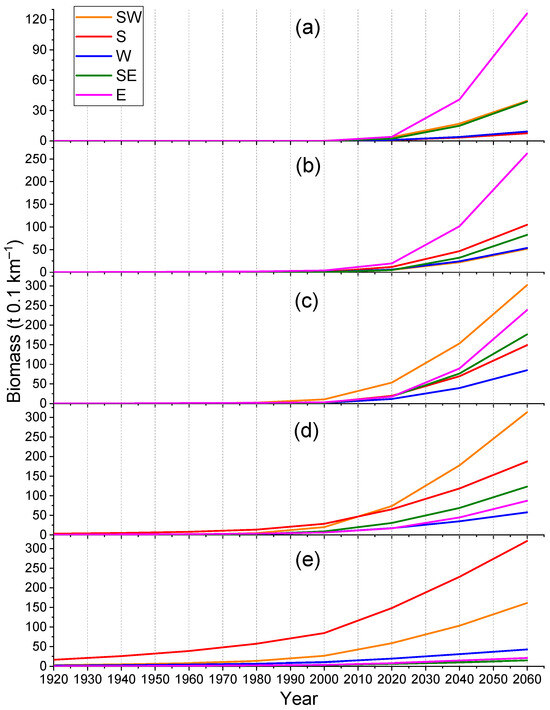
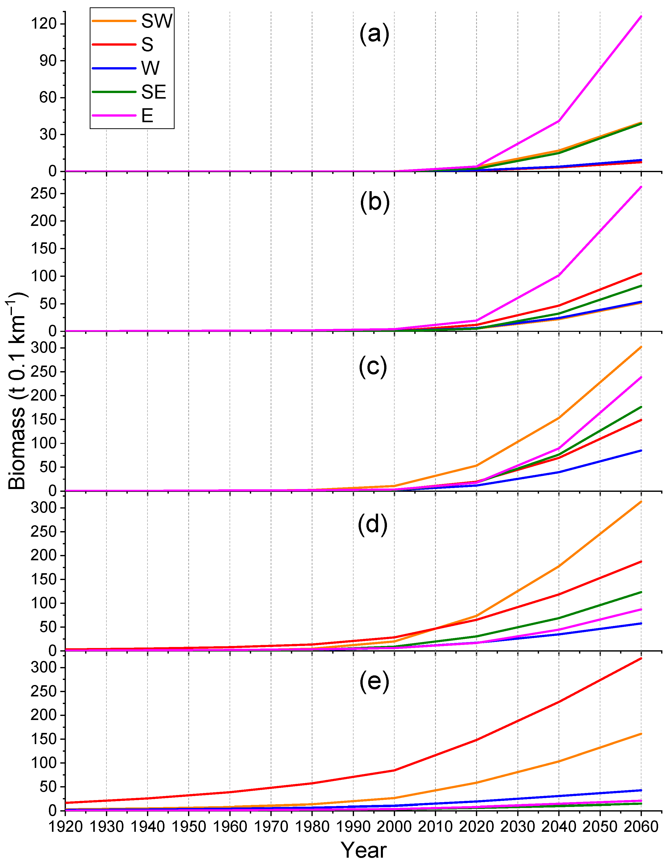

Disclaimer/Publisher’s Note: The statements, opinions and data contained in all publications are solely those of the individual author(s) and contributor(s) and not of MDPI and/or the editor(s). MDPI and/or the editor(s) disclaim responsibility for any injury to people or property resulting from any ideas, methods, instructions or products referred to in the content. |
© 2026 by the authors. Licensee MDPI, Basel, Switzerland. This article is an open access article distributed under the terms and conditions of the Creative Commons Attribution (CC BY) license.