


Abstract
Identifying suitable habitats for ecosystem restoration is critical for conserving globally threatened biodiversity. Baseline data on the distribution and range of biogenic habitat-forming species at high spatial resolution are essential for informing habitat management strategies and preserving ecosystem integrity. We identified suitable sites for habitat restoration by integrating community ecological data for Quercus mongolica Fisch. ex Turcz., a valuable restoration tree species, with insights from ensemble modeling. Habitat suitability was predicted using an ensemble species distribution model. A total of 89 occurrence records and nine environmental variables were used to develop the single algorithm models. Model performance was assessed using the Receiver Operating Characteristic (ROC) curve and the True Skill Statistic (TSS). Future habitat suitability was evaluated using projected climate change scenarios. Under more extreme climate change scenarios, the future suitable habitat of Q. mongolica is projected to gradually contract toward the high-altitude areas of Mt. Gariwang. The primary environmental variable is elevation, and rising temperatures due to climate change negatively impact habitat suitability for Q. mongolica. Therefore, adaptation measures must be established to mitigate these impacts, such as protecting the reference ecosystems of Q. mongolica. This integrated approach offers a nature-based solution for guiding climate change-integrated restoration programs in Mt. Gariwang and globally.
1. Introduction
Climate change and human activities significantly impact global biodiversity, habitats, and species extinctions [1,2,3]. The leading causes include land-use change, overexploitation, disruption of ecological interactions, and habitat alteration [4]. Human-induced climate change alters seasonal temperature and precipitation patterns in forest ecosystems, leading to extreme climatic events that affect the geographical or altitudinal distribution of land suitable for plant growth [5]. Consequently, changes in climatic conditions likely expand or reduce the geographical range of species [6]. Many native species have experienced significant changes in abundance and the seasonality of their activities [7]. These negative outcomes hinder habitat and biodiversity management, as well as ecosystem restoration.
Nature-based solutions, including the protection of natural ecosystems and the restoration of degraded ones, are considered sustainable strategies to address the global challenges of climate change and the biodiversity crisis [8]. The United Nations proclaimed 2021–2030 as the Decade on Ecosystem Restoration, emphasizing the need to protect existing ecosystems and restore degraded ones [9,10]. Restoration efforts should prioritize degraded ecosystems that are more likely to support biodiversity at high risk of extinction [11]. Species distribution modeling (SDM), which identifies suitable habitats and predicts range shifts under anticipated climate change, provides a promising tool for planning effective restoration strategies for endemic species at risk in biodiversity hotspots [12].
In recent years, ecosystems in South Korea have experienced significant degradation, particularly due to the destruction of approximately 78 hectares of forest on Mt. Gariwang for gondola construction and alpine ski resort development associated with the 2018 Winter Olympics [13]. In response, there has been growing interest in restoring degraded forest ecosystems, along with increased efforts to identify appropriate restoration approaches. Approaches based on the original state prior to degradation, such as utilizing reference ecosystems, are emerging [14]. Understanding the relationship between environmental and spatial factors is fundamental to biological and ecological conservation, making it essential to examine the distribution and dynamic responses of plant species along environmental gradients [15]. For instance, shifts in species distributions within forests can alter the spatial arrangement of vegetation zones, providing reference conditions for interpreting macroecological patterns, including projections of geographic range changes [16,17,18]. However, a comprehensive ecological and economic basis for restoring large-scale degraded areas lacks detailed data on the distribution and range of important ecosystems at local scales, as well as reference ecosystems for hotspots [19].
SDMs utilize discontinuous species occurrence records along with climate and environmental covariates to quantitatively predict potential habitat suitability for species across spatiotemporal gradients [20,21,22]. SDM projections can be integrated with future climate scenarios to forecast species distributions over time based on environmental suitability [23,24,25]. They can also inform sustainable management plans that mitigate the impacts of climate change [26,27,28]. However, uncertainties in SDMs, including limited spatial data, model limitations, and inaccuracies in climate change scenarios, have impeded the implementation of restoration plans [29,30,31]. To address these uncertainties, ensemble methodology based on consensus models has been employed [22]. This approach integrates various algorithms to enhance the accuracy of SDMs, providing a more reliable estimate for future species distributions [32].
Oak species are representative temperate deciduous broadleaf trees in South Korea, covering approximately 980,000 hectares [33]. Among them, Quercus mongolica has the largest distribution at 414,000 hectares [34]. Q. mongolica is a native species well-adapted to South Korea and is commonly used in ecological planting, constituting about 27% of the total domestic timber stock [35]. Its high sprout formation ability makes it prevalent in restoration sites, and it is reported to have significant tree biomass and carbon storage [36]. Thus, Q. mongolica is valuable as a restoration species and plays a crucial role in achieving carbon neutrality. However, a major challenge is the inadequate regeneration of dominant species, which hinders the evaluation of the restoration process.
Investigating habitat suitability of species is essential for understanding the impact of climate change on species distributions [37,38,39]. Thus, it is necessary to integrate climate change risks into biodiversity conservation strategies and ecosystem restoration practices [40,41]. In our study, we selected Q. mongolica at a high spatial resolution and regional scale, simulating potential habitat suitability distributions according to two scenarios (SSP245 and SSP585) of Shared Socioeconomic Pathways (SSP) through ensemble modeling. We aim to address the following key questions: (1) What is the current distribution of Q. mongolica? (2) What will be the future potential distribution of this species under different climate change scenarios? and (3) What key bioclimatic variables affect the distribution of this species?
2. Materials and Methods
2.1. Collection of Species Occurrence Data
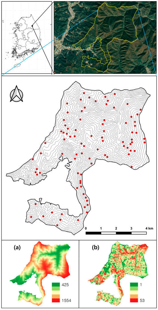
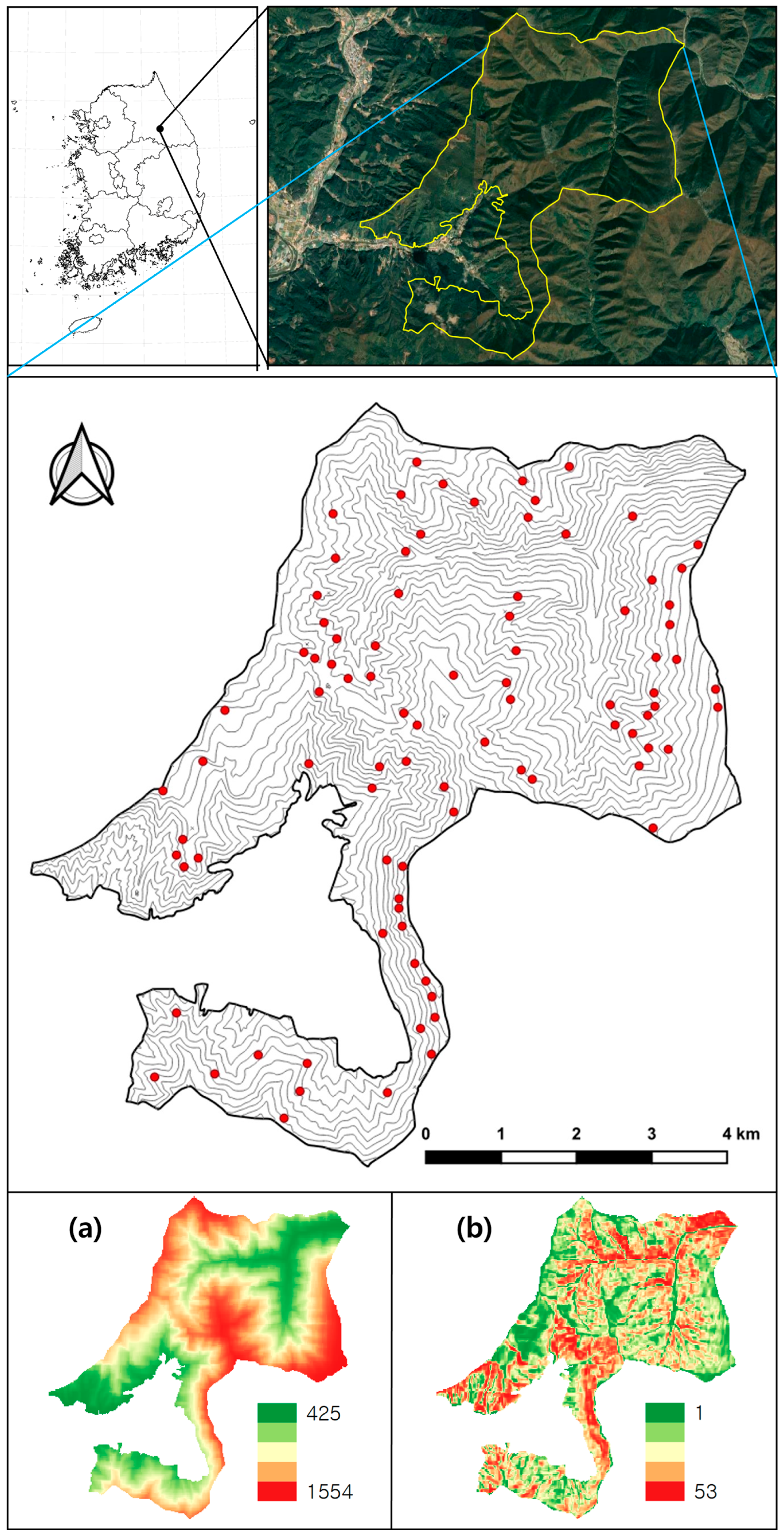
Q. mongolica identified on Mt. Gariwang was selected as the dominant species in the study area, with distribution points extracted from 89 locations (Figure 1). The variables were formatted as a CSV containing longitude and latitude in degrees. The longitude and latitude coordinates of Q. mongolica occurrence points were recorded in the field as Points of Interest (POI) using GPS. The performance of species distribution models (SDMs) can be influenced by the number of occurrence records used [42]. A smaller sample size may increase model accuracy; however, if the sample size is too large relative to the number of environmental variables, it can hinder model interpretation and increase the risk of overfitting [43,44,45]. Therefore, cross-validation was performed to ensure data integrity. POIs recorded in the field may be concentrated or duplicated, leading to spatially autocorrelated occurrence points that can distort species distribution probabilities [46,47]. To eliminate spatial autocorrelation from sampling bias, the data were preprocessed to include only one occurrence record per grid cell of the spatial variables. We included only georeferenced records from a three-year period (2018–2020), excluding clearly erroneous georeferences from the final dataset.
Figure 1.
Map of South Korea highlighting the study area (yellow boundary), displaying the selected occurrence points of Quercus mongolica (red dots) along with raster layers of elevation (a) and slope (b).
2.2. Selection of Environmental Variables
Vegetation is limited to specific areas, reflecting regional characteristics [48]. The environmental variables influencing the distribution of Q. mongolica include five topographic variables: elevation (DEM), aspect (ASPECT), slope (SLOPE), topographic position index (TPI), and topographic wetness index (TWI); and four climate variables: average temperature (Tavg), maximum temperature (Tmax), minimum temperature (Tmin), and average humidity (Havg).
Topographic variables were derived from a digital elevation model, which records the height values of points at regular intervals on the Earth’s surface, thereby representing terrain morphology in three dimensions. This includes spatial data for aspect, slope, the topographic position index, and the topographic wetness index. The topographic position index quantitatively represents the terrain’s relative position: a positive value indicates a ridge that is higher than its surroundings. In contrast, a negative value indicates a valley that is lower. The topographic wetness index quantitatively reflects terrain wetness: a lower value indicates less water accumulation during rainfall, whereas a higher value indicates more. Thus, smaller values of the topographic wetness index suggest drier soil environments, while larger values suggest wetter soil environments.
Climate variables affecting distribution and growth were derived from daily data collected by the domestic mountain meteorological network, with 30-year averages calculated from climate data spanning 1981–2010. Humidity data were used instead of precipitation data, as precipitation typically varies by region and shows little variation in small-scale areas. Additionally, humidity influences the forest environment and is closely related to the growth of adaptive plant species. Therefore, humidity data were prioritized.
Generally, terrestrial meteorological observations, such as the Automated Synoptic Observing System (ASOS), Automatic Weather System (AWS), and Agricultural Automated Observing System (AAOS), are not specifically designed for forest applications. Consequently, obtaining meteorological information in mountainous areas is challenging, resulting in decreased accuracy of the data. The mountain meteorological network data were adjusted using a correction factor based on the temperature lapse rate, representing the rate of temperature change with increasing elevation. Given that it accounts for mountainous areas and temperature lapse rates, this climate data is suitable for the study area.
The environmental variables must be selected to eliminate multicollinearity, which can negatively affect model creation due to variable correlation. However, due to the regional nature of the study area and the smaller number of variables compared to those commonly used in WorldClim, multicollinearity was not removed. The independent variable must be grid data in ASCII format, maintaining the same geographical range and spatial resolution. Accordingly, the spatial resolution was set to 30 m, and climate variables with coarser resolution were downscaled using the bilinear method.
To predict and compare future habitat distribution changes in Q. mongolica due to climate change, we selected the SSP scenario from the IPCC Assessment Report 6 (AR6). This SSP scenario considers mitigation and adaptation efforts to climate change based on socioeconomic changes and radiative forcing intensities, accounting for demographics, economic development, welfare, ecosystem factors, resources, and policies [49]. The optimistic scenario (SSP245) and the pessimistic scenario (SSP585) were selected to represent the extremes in climate change under scenarios of developed and reduced greenhouse gas emissions. The future climate time ranges are 2021–2040, 2041–2060, 2061–2080, and 2081–2100. Mean climate variable values for each time period were used to predict future habitat suitability, represented as the 2030s, 2050s, 2070s, and 2090s. The sources of topographic and climate variables are shown in the following table (Table 1).
Table 1.
Environmental predictors included in the species distribution model.
2.3. Development and Evaluation of the Species Distribution Model
Nine algorithms were employed to build the species distribution model: Artificial Neural Network (ANN), Generalized Additive Model (GAM), Generalized Linear Model (GLM), Generalized Boosting Regression Model (GBM), Classification Tree Analysis (CTA), Multiple Adaptive Regression Splines (MARS), Random Forest (RF), Maximum Entropy (MAXNET), and Surface Range Envelope (SRE) [50,51]. Except for Maxent and SRE, all models require binary input data in the form of presence–absence. In this study, 1000 pseudo-absence points were randomly sampled ten times, resulting in ten presence–absence datasets. Training and validation data were distinguished from each dataset at a 7:3 ratio, with 70% used for model creation and 30% for model accuracy evaluation. Each single algorithm model was executed ten times for each dataset using the environmental variables, and the contribution of each variable was calculated for every run. Model accuracy was assessed using ten-fold cross-validation.
For this purpose, validation data from each dataset were used to calculate the Receiver Operating Characteristic (ROC) curve and the True Skill Statistic (TSS) [52,53]. These criteria are commonly used in ecology to evaluate the performance of habitat modeling [52]. TSS assesses model performance based on the success rate of predicting presence and absence relative to a threshold. In contrast, ROC evaluates model performance across various thresholds to measure overall accuracy without relying on a single threshold. Sensitivity and specificity indicate how well the model predicts actual positive and negative data. The maximum sum of sensitivity and specificity was used to optimize the threshold in SDMs, allowing the conversion of continuous output into a binary factor for each SDM. Consequently, ROC was chosen as the evaluation criterion because its value is maximized when sensitivity and specificity are squared.
2.4. Prediction of Ensemble Model
Single algorithm models with ROC values of ≥0.6 were retained and integrated to build an ensemble model using the Committee Averaging (CA) method [54]. The CA method converts occurrence probabilities from each single-algorithm model into binary values (0 and 1), sums them across models, and then divides by the total number of models [51]. The CA ensemble model yields an intuitive, easy-to-compare output rather than a continuous variable [55]. Ensemble predictions are derived as a weighted average of individual model outputs, with weights assigned according to each model’s discriminative performance as indicated by the ROC [56]. To incorporate climate uncertainty, two scenarios (SSP245 and SSP585) were used to estimate the average occurrence probability for each time period [57]. Suitable habitats were defined by identifying the point on the ROC curve where sensitivity and specificity are optimally balanced, which was then used to set a threshold for each climate scenario and convert predictions into binary outcomes. Using the binarized maps, suitable habitat areas were classified into five categories based on predicted probabilities: 1. Unsuitable (p ≤ 0.20); 2. Low suitability (0.20 < p ≤ 0.40); 3. Moderate suitability (0.40 < p ≤ 0.60); 4. High suitability (0.60 < p ≤ 0.80); 5. Suitable (p > 0.80) [58]. We also calculated the total area (in km2) of suitable habitat for each climate change scenario based on binary predictions. The final models were projected into GIS to generate potential habitat maps. All analyses were conducted using the Biomod2 package [51] in the R program (ver. 4.3.2) [59].
3. Results
3.1. Performance Evaluation of Single Algorithm and Ensemble Models
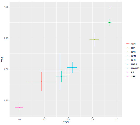
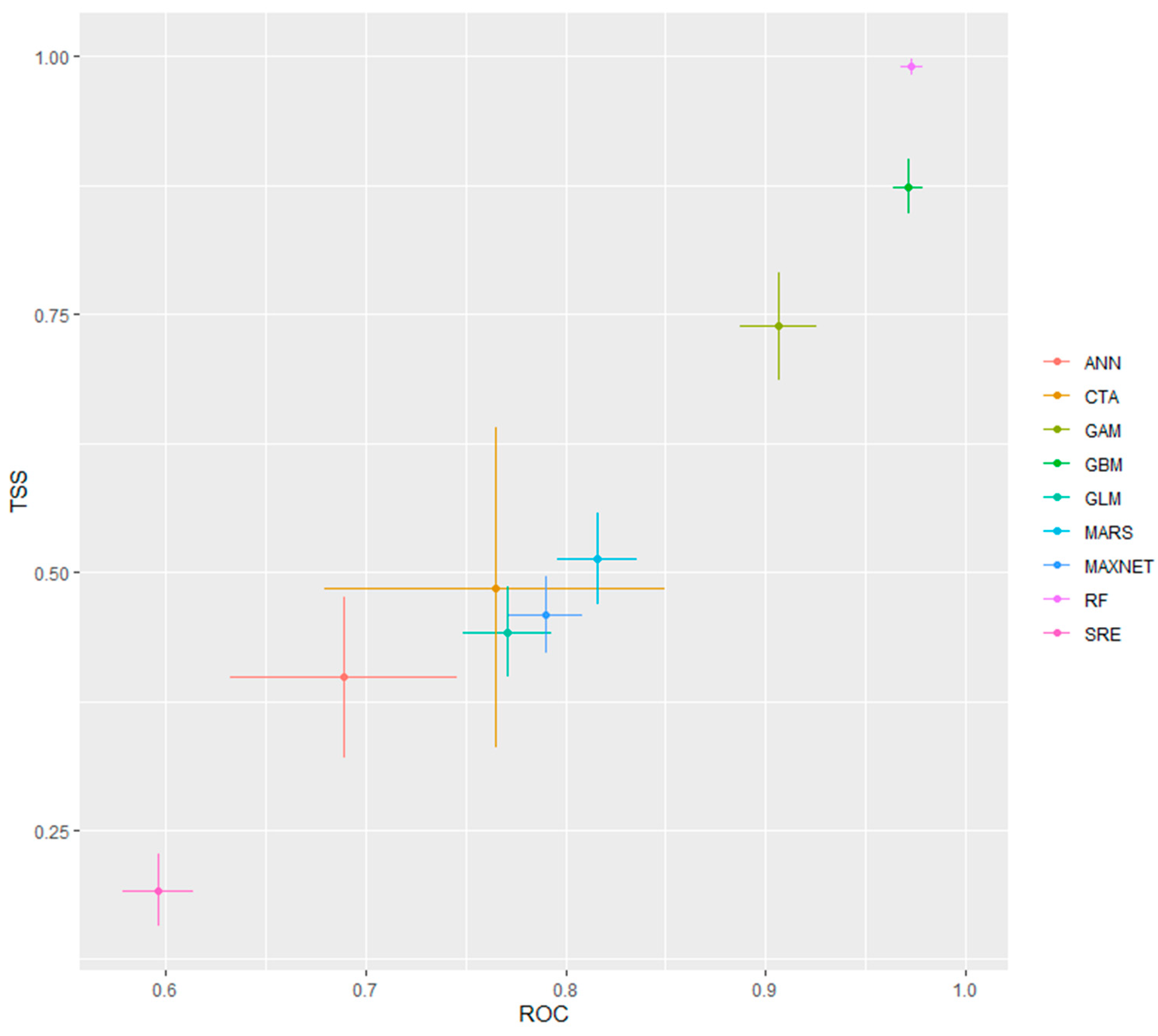
All algorithms employed in this study, with the exception of SRE, successfully predicted the presence of Q. mongolica (Figure 2). Across all single algorithm models, the mean ROC and TSS values were 0.82 ± 0.12 and 0.58 ± 0.25, respectively. Among the single-algorithm models, RF achieved the highest performance (ROC = 0.98 ± 0.01; TSS = 0.99 ± 0.01), followed by GBM, GAM, and MARS, whereas SRE showed the lowest predictive performance (ROC = 0.60 ± 0.02; TSS = 0.19 ± 0.04). The ensemble model, created from single algorithms with an ROC of ≥0.6, included 111 models (GAM, GBM, GLM, MARS, MAXNET, and RF), followed by 110 CTA models, 39 SRE models, and 15 ANN models. The ensemble model achieved ROC and TSS values of 0.93 and 0.71, respectively, indicating better predictive performance than the single algorithm models.
Figure 2.
Validation results for the single algorithm models, based on ROC and TSS. Points and crosses represent the mean values and corresponding standard deviations for each algorithm.
3.2. Habitat Suitability
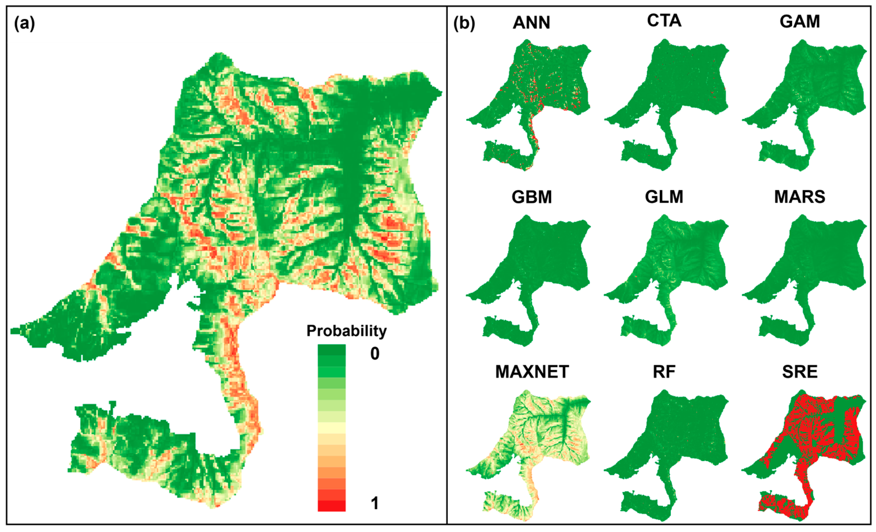
Under baseline climate conditions (1970–2000), the ensemble model estimated the suitable habitat area for Q. mongolica at 5,662,800 km2, with the highest suitability concentrated along central ridges and upper slopes (Figure 3a). The single algorithm models exhibited similar spatial patterns to the ensemble model, though there were differences in habitat suitability. Among the nine algorithms, GBM and MARS predicted low habitat suitability, whereas SRE indicated relatively higher suitability compared to the other models (Figure 3b).
Figure 3.
Baseline habitat suitability for Quercus mongolica (1981–2010) predicted by (a) the committee averaging ensemble model and (b) the single-algorithm models.
3.3. Environmental Variable Contribution
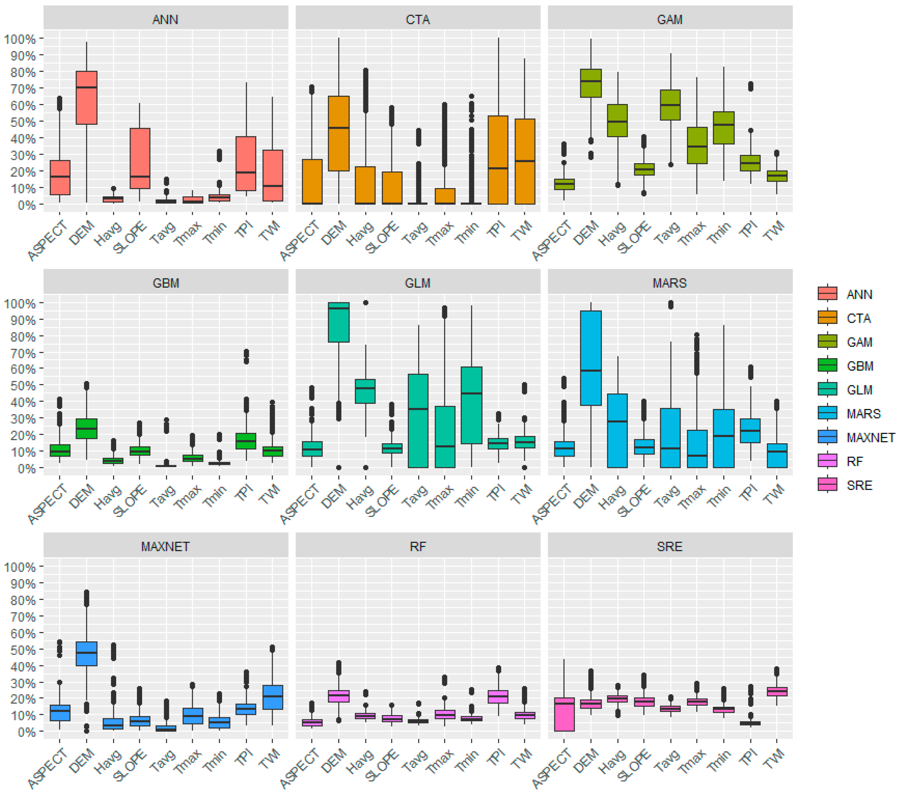
The environmental variable most associated with the occurrence of Q. mongolica was elevation (Figure 4). Elevation showed a variable importance of 0.46 ± 0.30 in the single algorithm models, making it the most influential predictor of Q. mongolica occurrence among the environmental variables used in the model. In the GLM algorithm model, the importance value for elevation was highest at 0.84–0.24, while the SRE algorithm model showed the lowest value at 0.17–0.04. Following elevation, average humidity showed a relatively high importance (mean = 0.21), exerting a greater influence on the occurrence of Q. mongolica than the other topographic variables. Climate variables such as average temperature, maximum temperature, and minimum temperature had importance values of 0.17, 0.15, and 0.18, respectively. Among topographical variables, the TWI and TPI contributed more than slope and aspect.
Figure 4.
Relative importance of nine environmental variables for predicting Quercus mongolica occurrence across single-algorithm models. Bars and error bars represent the mean importance values and their standard deviations for each algorithm.
3.4. Future Changes in Suitable Habitat
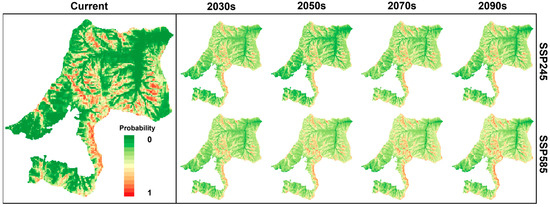
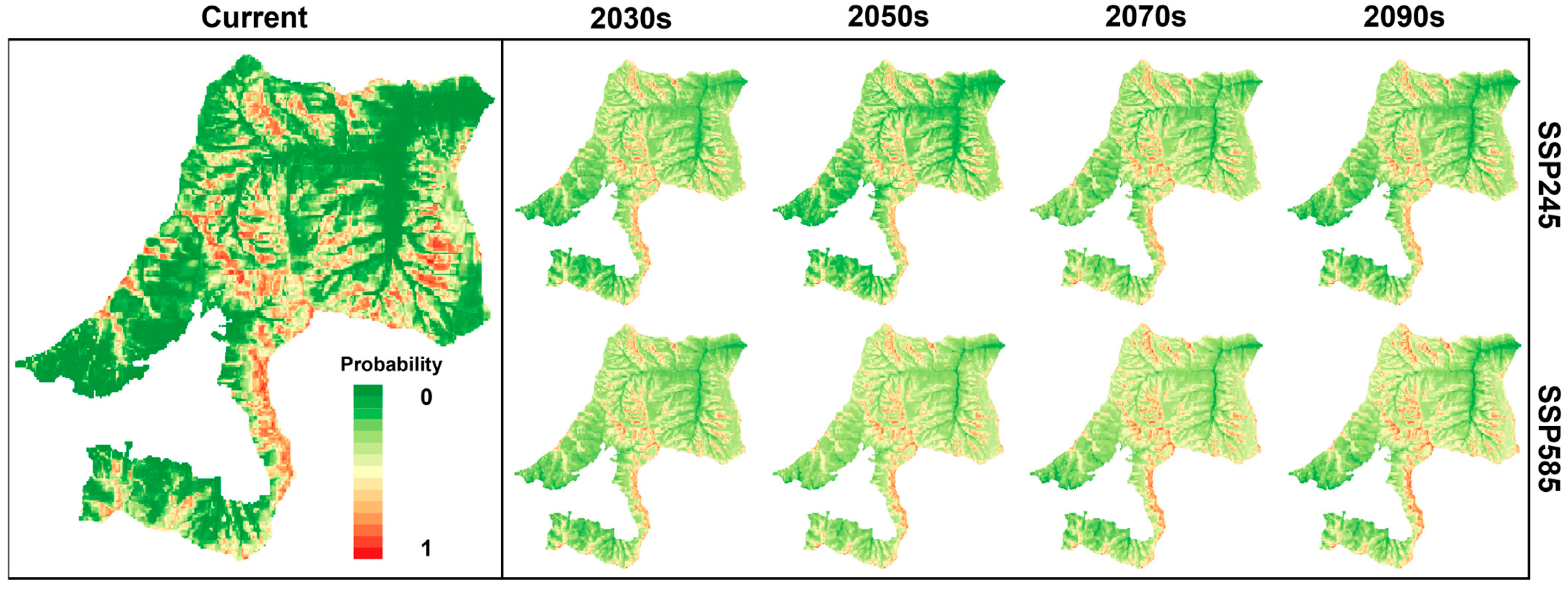
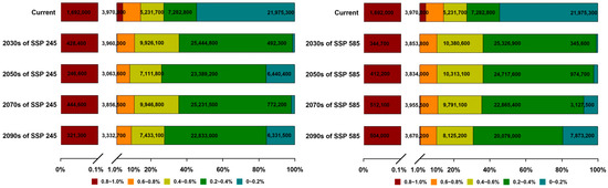
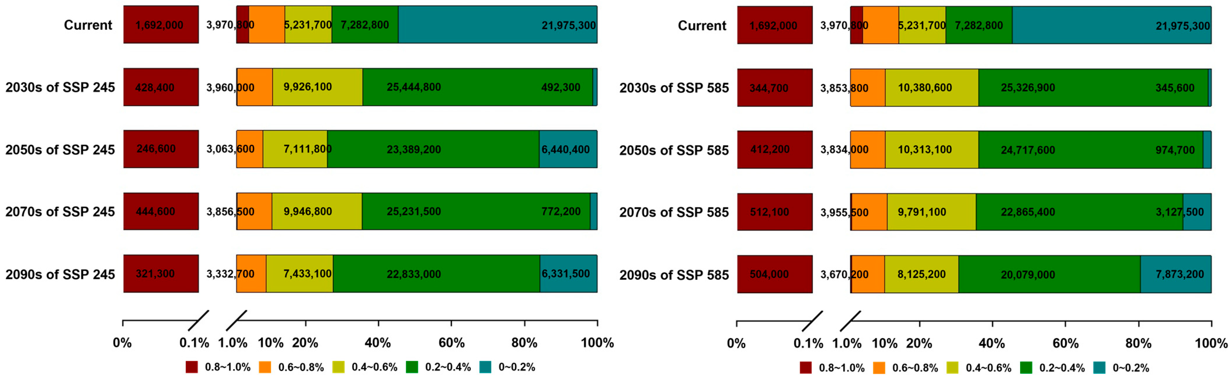
Under both SSP scenarios, habitat suitability declined in low-elevation and valley areas, becoming increasingly restricted to ridges, upper slopes, and higher elevations (Figure 5). Across all time periods, mean habitat suitability was consistently lower under the SSP245 scenario than under SSP585. For SSP245, habitat suitability in the 2050s and 2090s was 8.2% (3,310,200 km2) and 9.1% (3,654,000 km2), respectively, with differences of within 3% compared to earlier periods (Figure 6; Table 2). In contrast, unsuitability was high at 16.0% (6,440,400 km2) and 15.7% (6,331,500 km2) in the 2050s and 2090s, respectively. In the SSP585 scenario, both habitat suitability and unsuitability increased over time, particularly in the 2090s, when unsuitability accounted for one-fifth of the total (7,873,200 km2).
Figure 5.
Mean habitat suitability of Quercus mongolica under SSP245 and SSP585, estimated using the committee averaging ensemble approach.
Figure 6.
Change in potential distribution area for Quercus mongolica under the SSP245 and SSP585 scenarios.
Table 2.
Relative percentage changes compared to the absolute area of Quercus mongolica under the SSP245 and SSP585 scenarios (The unit is m2, and the value in parentheses is expressed as a percentage).
4. Discussion
We used an ensemble species distribution modeling approach to predict the future potential habitat of Q. mongolica under multiple climate change scenarios. The ensemble model constructed using the Committee Averaging method achieved ROC and TSS values of 0.93 and 0.71, respectively, demonstrating improved predictive performance compared to single algorithm models and reduced uncertainty through the integration of multiple algorithms [60,61]. Thus, the ensemble model’s predictions of Q. mongolica distribution provide preliminary guidance for identifying suitable habitats. Nevertheless, model evaluation was based on validation data drawn from the same dataset, which may limit the robustness of the ensemble model when extrapolated to independent temporal and spatial settings [62]. Additionally, optimizing the model parameters may yield better performance from a single algorithm model compared to the ensemble model using default settings. Accordingly, reliable evaluation of ensemble model performance requires supplementary approaches, including null model testing or external validation, in addition to internal validation [63,64]. Future studies should assess model performance using spatial blocking approaches or independent validation data [63]. Furthermore, reducing overfitting in single algorithm models through parameter optimization may enhance the ensemble model’s accuracy and transferability [65]. The high ROC and TSS values observed in this study demonstrate the usefulness of the ensemble approach; however, these performance metrics are based on internal validation derived from the same data source and therefore do not directly guarantee spatial or temporal transferability. In addition, the use of pseudo-absence data, the presence of multicollinearity among environmental predictors, the downscaling of coarse-resolution climate data, and the inherent uncertainty in future climate scenarios may all influence prediction reliability. Accordingly, while the model is useful for identifying the relative priority of potential restoration areas for Q. mongolica, further improvements—such as spatial block cross-validation, independent validation datasets, refined variable selection, and explicit assessment of uncertainty across climate models—are required for robust, site-specific restoration decision-making.
Among the nine algorithms evaluated, Random Forest (RF) showed the highest accuracy in predicting the occurrence of Q. mongolica. This strong predictive performance of RF is supported by previous comparative studies [66,67], including research in South Korea on subalpine evergreen conifers that also reported high performance for RF alongside GBM [68]. RF is a machine learning technique that generates multiple decision trees and combines their predictions, preventing overfitting by ensuring diversity through bootstrap sampling and random variable selection [69]. It effectively handles interactions and nonlinearities between influential factors, maintaining robust performance even in the presence of missing values and outliers [70,71]. Thus, RF serves as a valuable tool for interpreting complex ecosystem or environmental data. Giving priority to RF results alongside the ensemble model when identifying suitable habitats for Q. mongolica improves the reliability of decision-making. All other algorithms, apart from SRE, demonstrated satisfactory predictive performance based on ROC and TSS and were therefore included in identifying suitable habitats for Q. mongolica. This approach helps capture ecological information that the ensemble model might overlook by preserving the unique ecological relationships represented in each individual algorithm [65]. In contrast, SRE’s ROC and TSS values were low, and domestic research has confirmed its lower accuracy compared to other algorithms [72]. Consequently, caution is warranted when using the SRE algorithm in ensemble model creation.
Q. mongolica is a dominant species in various ecosystems throughout the Northern Hemisphere, particularly on the Korean Peninsula, Japan, northeastern China, and Siberia [73]. Its natural habitats include high mountain ridges and slopes at elevations of 100–1800 m in South Korea, with the highest occurrence around 700 m above sea level [74]. This study identified several variables relevant to Q. mongolica based on reference conditions, including DEM, Havg, TPI, and TWI, which are critical for determining potential distribution areas. These variables indicate that Q. mongolica is closely associated with suitable locations, soil conditions, humidity, and elevation. Specifically, Q. mongolica thrives in dry soil environments, high slopes, and ridge locations rather than moist soil [75]. This aligns with Jeong et al. [76], who classified Q. mongolica as a xerophytic growth species. The species is primarily distributed at elevations of 800–1000 m, with habitat suitability highest when the average humidity is between 58% and 62% [75]. Understanding the relationships between the variables and the ecological and biological factors that define the species’ range is essential for evaluating the model’s significance. Elevation correlates with temperature, indirectly influencing the growth, reproduction, and distribution of Q. mongolica through general environmental conditions [77]. However, the results indicated that the temperature index and slope had lower importance than other variables. This low significance may result from the coarse spatial resolution of these variables, which fails to capture fine temperature variations adequately. Accordingly, further research is needed to clarify how temperature conditions influence the growth and distribution of Q. mongolica.
The ensemble model indicates that, under both SSP245 and SSP585 scenarios, the suitable habitat for Q. mongolica progressively shifts to higher elevations in mountainous regions from the near to the distant future. Climate change has resulted in alterations in geographic distribution, characterized by both expansion and contraction. Across all utilization scenarios, the overall habitat suitability (i.e., the sum of high, moderate, and low suitability areas) is expected to decrease [78]. Notably, habitat unsuitability peaks in the 2050s and 2090s of SSP245 due to greater changes in radiative forcing during these decades, which increase climate sensitivity to conditions such as temperature, precipitation, wind, and humidity [49]. This rise in radiative forcing exacerbates the energy imbalance in the Earth’s climate system, leading to changes in climate factors such as rising atmospheric temperatures and altered precipitation patterns, which significantly affect the physiological and ecological responses of plants [79]. This may result in decreased photosynthetic efficiency from high temperatures, water stress from increased transpiration, and shorter growing periods, as well as ecosystem-level changes such as diminished biodiversity, geographical shifts in species distribution, and the spread of pests and diseases [80]. These changes critically impact vegetation composition and ecosystem function, necessitating quantitative predictions of plant responses to radiative forcing and the development of ecological adaptation strategies. The SSP585 scenario in the 2090s shows the largest area decrease of 7,873,200 km2. These outcomes can lead to species extinctions, demographic changes, shifts in phenology, and variations in growth and productivity under future climate scenarios [81]. According to Monzón et al. [82], climate change can drive species ranges to either expand or contract, and some species may need to shift their distributions to occupy newly suitable environments [78]. Consequently, under the pessimistic SSP585 scenario, Q. mongolica is predicted to have a greater potential for emergence and persistence within its existing habitat, even under extreme climate change, compared to the optimistic SSP245 scenario. Lee et al. [83] also predicted that Q. mongolica would maintain a certain level of suitable habitat, particularly at high altitudes, despite ongoing warming due to climate change.
The projected contraction of suitable habitat toward high-elevation ridges and upper slopes has important implications for the long-term feasibility of restoration. In particular, our results suggest that restoration planning should move beyond present-day suitability and instead focus on climatic persistence under future scenarios. Sites that are currently suitable may become progressively less stable for Q. mongolica establishment, regeneration, and long-term stand maintenance under continued warming. In contrast, high-elevation areas may serve as climate refugia and thus represent strategic priorities for long-term restoration and conservation. From this perspective, restoration should be framed not simply as re-establishing historical vegetation, but as promoting self-sustaining forest ecosystems that remain viable under future climate conditions. In particular, climate niche shift, range contraction, and upslope migration are presented as the climate-adaptive restoration framework as factors explaining the core patterns of restoration ecology in the era of climate change. Although uncertainty remains in the ensemble predictions, the model provides a practical basis for reducing restoration risk, identifying robust restoration sites, and supporting climate-adaptive restoration planning.
5. Conclusions
We were able to provide relatively clear answers to the research questions presented in the Introduction. The potential distribution of Q. mongolica predicted under current climatic conditions showed high habitat suitability mainly along the middle ridges and upper slopes of mountainous areas. In particular, the suitable habitat area was estimated at 5,662,800 km2, and all algorithms used in this study, except SRE, appropriately predicted the presence of Q. mongolica. The predictions of potential distribution under future climate change scenarios showed a tendency for habitat suitability to gradually shift toward higher elevations over time. From the near future to the distant future, habitat suitability is projected to decrease in lowland and valley areas, while relatively high suitability is maintained in higher-elevation locations such as mountain ridges and upper slopes. Mean habitat suitability was lower under the SSP245 scenario than under the SSP585 scenario across all time periods. Among the environmental variables used, elevation was identified as the most important explanatory variable, followed by average humidity, the topographic position index, and the topographic wetness index. These variables indicate that the distribution of Q. mongolica is shaped by a complex interaction of suitable site conditions, soil environment, humidity, and elevation.
Our results provide the first comprehensive overview of potential habitats within Mt. Gariwang, identifying previously unknown areas beyond the known distribution. This knowledge is valuable for informing focused restoration efforts for species globally. Additionally, this ecologically significant species serves as an indicator of ecosystem health and plays a crucial role in restoring degraded ecosystems. Models can provide valuable insights into the potential for species restoration, which is crucial for both in situ and ex situ conservation, as well as forest management. Efforts to model the species’ potential habitats present new opportunities for research and restoration in South Korea. This model can also be applied in other regions of the species’ distribution range to clarify global habitat availability, aiding in the estimation of potential habitats worldwide.
Achieving restoration goals requires swiftly identifying suitable habitats at multiple spatial scales and finding solutions relevant to local decision-makers and restoration projects. The success of restoration efforts hinges on securing ecological connectivity, emphasizing the need to define extensive areas of suitable habitat. This study advocates for an integrated approach prioritizing habitat restoration and accurately identifying favorable reintroduction sites based on climate change projections. Assessing species occurrence both within and outside natural environments will support restoration initiatives. Modeling species distributions can serve as an early warning system, flagging potential habitat changes resulting from climate change. This data will help forest planners and environmental organizations select optimal locations for future restoration efforts.
SDM-based predictions of species distribution range changes due to climate change provide valuable information for forest ecosystem restoration and management. However, the predictive accuracy of SDMs is limited by various factors, introducing uncertainty into planning. SDM simulation results, influenced by algorithm and parameter selection, can be somewhat managed through multi-model ensemble modeling. Nonetheless, sampling bias in observation points and inherent uncertainties in environmental variables, such as future climate data, can create additional uncertainty in habitat distribution predictions. Mountainous regions with significant interregional weather differences, like those in South Korea, require higher-resolution local data. Therefore, integrating insights from regional-scale community ecology, which has largely remained an isolated research area, with macro spatial scale SDM could enhance the design of successful restoration strategies.
Author Contributions
Conceptualization, investigation, analysis, visualization, writing, and original draft preparation, M.K.; supervision, curation, and editing, N.K.; review, Y.S., K.L., A.R.K., J.-H.C. and N.K. All authors have read and agreed to the published version of the manuscript.
Funding
This research was funded by the National Institute of Forest Science (grant number: FE0100-2024-04-2026).
Institutional Review Board Statement
Not applicable.
Data Availability Statement
The data presented in this study are available upon request from the corresponding author. The data are not publicly available due to privacy concerns.
Conflicts of Interest
The authors declare no conflicts of interest.
References
- Bejagam, V.; Sharma, A. Impact of climatic changes and anthropogenic activities on ecosystem net primary productivity in India during 2001–2019. Ecol. Inform. 2022, 70, 101732. [Google Scholar] [CrossRef] [Scilit]
- Haines, A.; Patz, J.A. Health effects of climate change. JAMA 2004, 291, 99–103. [Google Scholar] [CrossRef] [Scilit] [PubMed]
- Learmonth, J.A.; MacLeod, C.D.; Santos, M.B.; Pierce, G.J.; Crick, H.Q.P.; Robinson, R.A. Potential effects of climate change on marine mammals. In Oceanography and Marine Biology; Gibson, R., Atkinson, R., Gordon, J., Eds.; CRC Press: Boca Raton, FL, USA, 2006; pp. 431–464. [Google Scholar] [CrossRef] [Scilit]
- IPBES. Global Assessment Report on Biodiversity and Ecosystem Services of the Intergovernmental Science-Policy Platform on Biodiversity and Ecosystem Services; IPBES Secretariat: Bonn, Germany, 2019. [Google Scholar]
- Bailey, R.G. Ecosystem Geography: From Ecoregions to Sites, 2nd ed.; Springer: New York, NY, USA, 2009. [Google Scholar]
- Chen, I.C.; Hill, J.K.; Ohlemüller, R.; Roy, D.B.; Thomas, C.D. Rapid range shifts of species associated with high levels of climate warming. Science 2011, 333, 1024–1026. [Google Scholar] [CrossRef] [Scilit] [PubMed]
- Weiskopf, S.R.; Rubenstein, M.A.; Crozier, L.G.; Gaichas, S.; Griffis, R.; Halofsky, J.E.; Hyde, K.J.W.; Morelli, T.L.; Morisette, J.T.; Muñoz, R.C.; et al. Climate change effects on biodiversity, ecosystems, ecosystem services, and natural resource management in the United States. Sci. Total Environ. 2020, 733, 137782. [Google Scholar] [CrossRef] [Scilit]
- The IUCN Red List of Threatened Species Home Page. Available online: https://www.iucnredlist.org (accessed on 29 June 2021).
- Fischer, J.; Riechers, M.; Loos, J.; Martin-Lopez, B.; Temperton, V.M. Making the UN decade on ecosystem restoration a social-ecological endeavour. Trends Ecol. Evol. 2021, 36, 20–28. [Google Scholar] [CrossRef] [Scilit]
- Abhilash, P.C. Restoring the unrestored: Strategies for restoring global land during the UN decade on ecosystem restoration (UN-DER). Land 2021, 10, 201. [Google Scholar] [CrossRef] [Scilit]
- Padilla, F.M.; Pugnaire, F.I. The role of nurse plants in the restoration of degraded environments. Front. Ecol. Environ. 2006, 4, 196–202. [Google Scholar] [CrossRef] [Scilit]
- Rather, Z.A.; Ahmad, R.; Dar, T.U.H.; Khuroo, A.A. Ensemble modelling enables identification of suitable sites for habitat restoration of threatened biodiversity under climate change: A case study of Himalayan Trillium. Ecol. Eng. 2022, 176, 106534. [Google Scholar] [CrossRef] [Scilit]
- Jeon, D.U.; Chon, J. System thinking in the resilience of the ecosystem and ecotourism of Mt. Gariwang based on the controversy around the venue construction for Pyeongchang 2018 Olympic. Korean Syst. Dyn. Rev. 2014, 15, 61–79. [Google Scholar]
- Kim, M.; Koo, N.; Kim, A.R.; Lee, K.; Yun, S.J. Reference ecosystem condition-based syntaxonomic study for ecological restoration and protection of temperate forests in South Korea. Diversity 2025, 17, 40. [Google Scholar] [CrossRef] [Scilit]
- Franklin, J. Mapping Species Distributions: Spatial Inference and Prediction; Cambridge University Press: Cambridge, UK, 2010. [Google Scholar] [CrossRef] [Scilit]
- Fitzpatrick, M.C.; Gove, A.D.; Sanders, N.J.; Dunn, R.R. Climate change, plant migration, and range collapse in a global Biodiversity Hotspot: The Banksia (Proteaceae) of Western Australia. Glob. Change Biol. 2008, 14, 1337–1352. [Google Scholar] [CrossRef] [Scilit]
- Lawler, J.J.; Shafer, S.L.; White, D.; Kareiva, P.; Maurer, E.P.; Blaustein, A.R.; Bartlein, P.J. Projected climate-induced faunal change in the Western Hemisphere. Ecology 2009, 90, 588–597. [Google Scholar] [CrossRef] [Scilit] [PubMed]
- Mateo, R.G.; Felicísimo, Á.M.; Pottier, J.; Guisan, A.; Muñoz, J. Do stacked species distribution models reflect altitudinal diversity patterns? PLoS ONE 2012, 7, e32586. [Google Scholar] [CrossRef] [Scilit]
- Bellard, C.; Bertelsmeier, C.; Leadley, P.; Thuiller, W.; Courchamp, F. Impacts of climate change on the future of biodiversity. Ecol. Lett. 2012, 15, 365–377. [Google Scholar] [CrossRef] [Scilit] [PubMed]
- Guisan, A.; Zimmermann, N.E. Predictive habitat distribution models in ecology. Ecol. Modell. 2000, 135, 147–186. [Google Scholar] [CrossRef] [Scilit]
- Elith, J.; Graham, C.H.; Anderson, R.P.; Dudík, M.; Ferrier, S.; Guisan, A.; Hijmans, R.J.; Huettmann, F.; Leathwick, J.R.; Lehmann, A.; et al. Novel methods improve prediction of species’ distributions from occurrence data. Ecography 2006, 29, 129–151. [Google Scholar] [CrossRef] [Scilit]
- Ahmad, R.; Khuroo, A.A.; Charles, B.; Hamid, M.; Rashid, I.; Aravind, N.A. Global distribution modelling, invasion risk assessment and niche dynamics of Leucanthemum vulgare (Ox-eye Daisy) under climate change. Sci. Rep. 2019, 9, 11395. [Google Scholar] [CrossRef] [Scilit]
- Elith, J.; Kearney, M.; Phillips, S. The art of modelling range-shifting species. Methods Ecol. Evol. 2010, 1, 330–342. [Google Scholar] [CrossRef] [Scilit]
- Franklin, J. Moving beyond static species distribution models in support of conservation biogeography. Divers. Distrib. 2010, 16, 321–330. [Google Scholar] [CrossRef] [Scilit]
- Sill, S.R.; Dawson, T.P. Climate change impacts on the ecological dynamics of two coral reef species, the humphead wrasse (Cheilinus undulatus) and crown-of-thorns starfish (Ancanthaster planci). Ecol. Inform. 2021, 65, 101399. [Google Scholar] [CrossRef] [Scilit]
- Pyke, C.R.; Fischer, D.T. Selection of bioclimatically representative biological reserve systems under climate change. Biol. Conserv. 2005, 121, 429–441. [Google Scholar] [CrossRef] [Scilit]
- Schorr, G.; Holstein, N.; Pearman, P.B.; Guisan, A.; Kadereit, J.W. Integrating species distribution models (SDMs) and phylogeography for two species of Alpine Primula. Ecol. Evol. 2012, 2, 1260–1277. [Google Scholar] [CrossRef] [Scilit]
- Porfirio, L.L.; Harris, R.M.B.; Lefroy, E.C.; Hugh, S.; Gould, S.F.; Lee, G.; Bindoff, N.L.; Mackey, B. Improving the use of species distribution models in conservation planning and management under climate change. PLoS ONE 2014, 9, e113749. [Google Scholar] [CrossRef] [Scilit] [PubMed]
- Flather, C.H.; Wilson, K.R.; Dean, D.J.; McComb, W.C. Identifying gaps in conservation networks of indicators and uncertainty in geographic-based analyses. Ecol. Appl. 1997, 7, 531–542. [Google Scholar] [CrossRef]
- Araújo, M.B.; Whittaker, R.J.; Ladle, R.J.; Erhard, M. Reducing uncertainty in projections of extinction risk from climate change. Glob. Ecol. Biogeogr. 2005, 14, 529–538. [Google Scholar] [CrossRef] [Scilit]
- Elith, J.; Leathwick, J.R. Species distribution models: Ecological explanation and prediction across space and time. Annu. Rev. Ecol. Evol. Syst. 2009, 40, 677–697. [Google Scholar] [CrossRef] [Scilit]
- Zhang, K.; Zhang, Y.; Jia, D.; Tao, J. Species distribution modeling of sassafras Tzumu and implications for forest management. Sustainability 2020, 12, 4132. [Google Scholar] [CrossRef] [Scilit]
- Park, J.H.; Chung, S.H.; Kim, S.H.; Lee, S.T. Estimation of site index curve for 6 oak species in Korea. J. Agric. Life Sci. 2020, 54, 27–33. [Google Scholar] [CrossRef] [Scilit]
- Lee, S.J.; Yim, J.S.; Son, Y.M.; Son, Y.; Kim, R. Estimation of forest carbon Stocks for national greenhouse gas inventory reporting in South Korea. Forests 2018, 9, 625. [Google Scholar] [CrossRef] [Scilit]
- Lee, S.W.; Won, H.K.; Shin, M.Y.; Son, Y.M.; Lee, Y.Y. Estimation of forest productive area of Quercus acutissima and Quercus mongolica using site environmental variables. Korean J. Soil Sci. Fertil. 2007, 40, 429–434. [Google Scholar]
- Lee, S.T.; Chung, S.H.; Kim, C. Carbon Stocks in Tree Biomass and Soils of Quercus acutissima, Q. mongolica, Q. serrata, and Q. variabilis stands. J. Korean Soc. For. Sci. 2022, 111, 365–373. [Google Scholar]
- Barbosa, F.G. The future of invasive African grasses in South America under climate change. Ecol. Inform. 2016, 36, 114–117. [Google Scholar] [CrossRef] [Scilit]
- Chiu-Valderrama, J.I.; Siurob-Espíndola, B.E.; Zúñiga-Vega, J.J.; de la Vega-Pérez, A.H.D.; Canales-Gordillo, B.; Jaramillo-Alba, J.L.; Akcali, C.K.; Cuervo-Robayo, A.P.; Pérez-Mendoza, H.A. Nowhere to go: Potential distribution shifts of a widespread lizard under two climate change scenarios. Ecol. Inform. 2022, 70, 101735. [Google Scholar] [CrossRef] [Scilit]
- Guan, B.C.; Guo, H.J.; Chen, S.S.; Li, D.M.; Liu, X.; Gong, X.; Ge, G. Shifting ranges of eleven invasive alien plants in China in the face of climate change. Ecol. Inform. 2020, 55, 101024. [Google Scholar] [CrossRef] [Scilit]
- Mehta, P.; Bisht, K.; Sekar, K.C. Diversity of threatened medicinal plants of Indian Himalayan Region. Plant Biosyst. 2021, 155, 1121–1132. [Google Scholar] [CrossRef] [Scilit]
- Mehta, P.; Sekar, K.C.; Bhatt, D.; Tewari, A.; Bisht, K.; Upadhyay, S.; Negi, V.S.; Soragi, B. Conservation and prioritization of threatened plants in Indian Himalayan Region. Biodivers. Conserv. 2020, 29, 1723–1745. [Google Scholar] [CrossRef] [Scilit]
- Wisz, M.S.; Hijmans, R.J.; Li, J.; Peterson, A.T.; Graham, C.H.; Guisan, A.; NCEAS Predicting Species Distributions Working Group. Effects of sample size on the performance of species distribution models. Divers. Distrib. 2008, 14, 763–773. [Google Scholar] [CrossRef] [Scilit]
- ter Steege, H.T.; Haripersaud, P.P.; Bánki, O.S.; Schieving, F. A model of botanical collectors’ behavior in the field: Never the same species twice. Am. J. Bot. 2011, 98, 31–37. [Google Scholar] [CrossRef] [Scilit]
- McPherson, J.M.; Jetz, W.; Rogers, D.J. The effects of species’ range sizes on the accuracy of distribution models: Ecological phenomenon or statistical artefact? J. Appl. Ecol. 2004, 41, 811–823. [Google Scholar] [CrossRef] [Scilit]
- Kramer-Schadt, S.; Niedballa, J.; Pilgrim, J.D.; Schröder, B.; Lindenborn, J.; Reinfelder, V.; Stillfried, M.; Heckmann, I.; Scharf, A.K.; Augeri, D.M.; et al. The importance of correcting for sampling bias in MaxEnt species distribution models. Divers. Distrib. 2013, 19, 1366–1379. [Google Scholar] [CrossRef] [Scilit]
- Naimi, B.; Skidmore, A.K.; Groen, T.A.; Hamm, N.A.S. Spatial autocorrelation in predictors reduces the impact of positional uncertainty in occurrence data on species distribution modelling. J. Biogeogr. 2011, 38, 1497–1509. [Google Scholar] [CrossRef] [Scilit]
- Warren, D.L.; Seifert, S.N. Ecological niche modeling in Maxent: The importance of model complexity and the performance of model selection criteria. Ecol. Appl. 2011, 21, 335–342. [Google Scholar] [CrossRef] [Scilit] [PubMed]
- Kim, N.S.; Han, D.; Cha, J.Y.; Kwon, H.J.; Cho, Y.C.; Oh, S.H.; Yoo, S.H.; Yu, D.S.; Park, Y.S. A study on geotop classification and geodiversity in Mt. Jeombong experimental forest. J. Korean Soc. Environ. Restor. Technol. 2015, 18, 179–190. [Google Scholar] [CrossRef] [Scilit]
- Tebaldi, C.; Debeire, K.; Eyring, V.; Fischer, E.; Fyfe, J.; Friedlingstein, P.; Knutti, R.; Lowe, J.; O’Neill, B.; Sanderson, B.; et al. Climate model projections from the Scenario Model Intercomparison Project (ScenarioMIP) of CMIP6. Earth Syst. Dyn. 2021, 12, 253–293. [Google Scholar] [CrossRef] [Scilit]
- Heikkinen, R.K.; Luoto, M.; Araújo, M.B.; Virkkala, R.; Thuiller, W.; Sykes, M.T. Methods and uncertainties in bioclimatic envelope modelling under climate change. Prog. Phys. Geogr. 2006, 30, 751–777. [Google Scholar] [CrossRef] [Scilit]
- Thuiller, W.; Lafourcade, B.; Engler, R.; Araújo, M.B.; BIOMOD. BIOMOD—A platform for ensemble forecasting of species distributions. Ecography 2009, 32, 369–373. [Google Scholar] [CrossRef] [Scilit]
- Allouche, O.; Tsoar, A.; Kadmon, R. Assessing the accuracy of species distribution models: Prevalence, kappa and the true skill statistic (TSS). J. Appl. Ecol. 2006, 43, 1223–1232. [Google Scholar] [CrossRef] [Scilit]
- Wani, I.A.; Khan, S.; Verma, S.; Al-Misned, F.A.; Shafik, H.M.; El-Serehy, H.A. Predicting habitat suitability and niche dynamics of Dactylorhiza hatagirea and Rheum webbianum in the Himalaya under projected climate change. Sci. Rep. 2022, 12, 13205. [Google Scholar] [CrossRef] [Scilit]
- Häkkinen, H.; Petrovan, S.O.; Sutherland, W.J.; Pettorelli, N. Terrestrial or marine species distribution model: Why not both? A case study with seabirds. Ecol. Evol. 2021, 11, 16634–16646. [Google Scholar] [CrossRef] [Scilit]
- Gallien, L.; Douzet, R.; Pratte, S.; Zimmermann, N.E.; Thuiller, W. Invasive species distribution models—How violating the equilibrium assumption can create new insights. Glob. Ecol. Biogeogr. 2012, 21, 1126–1136. [Google Scholar] [CrossRef] [Scilit]
- Quinci, E.M.; Torri, M.; Cuttitta, A.; Patti, B. Predicting potential spawning habitat by ensemble species distribution models: The case study of European anchovy (Engraulis encrasicolus) in the Strait of Sicily. Water 2022, 14, 1400. [Google Scholar] [CrossRef] [Scilit]
- Koo, K.A.; Park, S.U.; Kong, W.S.; Hong, S.; Jang, I.; Seo, C. Potential climate change effects on tree distributions in the Korean Peninsula: Understanding model & climate uncertainties. Ecol. Modell. 2017, 353, 17–27. [Google Scholar] [CrossRef] [Scilit]
- Awan, M.N.; Saqib, Z.; Buner, F.; Lee, D.C.; Pervez, A. Using ensemble modeling to predict breeding habitat of the red-listed Western Tragopan (Tragopan melanocephalus) in the Western Himalayas of Pakistan. Glob. Ecol. Conserv. 2021, 31, e01864. [Google Scholar] [CrossRef] [Scilit]
- R Core Team. A Language and Environment for Statistical Computing; R Foundation for Statistical Computing: Vienna, Austria, 2022. [Google Scholar]
- Araújo, M.B.; New, M. Ensemble forecasting of species distributions. Trends Ecol. Evol. 2007, 22, 42–47. [Google Scholar] [CrossRef] [Scilit] [PubMed]
- Marmion, M.; Parviainen, M.; Luoto, M.; Heikkinen, R.K.; Thuiller, W. Evaluation of consensus methods in predictive species distribution modelling. Divers. Distrib. 2009, 15, 59–69. [Google Scholar] [CrossRef] [Scilit]
- Crimmins, S.M.; Dobrowski, S.Z.; Mynsberge, A.R. Evaluating ensemble forecasts of plant species distributions under climate change. Ecol. Modell. 2013, 266, 126–130. [Google Scholar] [CrossRef] [Scilit]
- Hao, T.; Elith, J.; Lahoz-Monfort, J.J.; Guillera-Arroita, G. Testing whether ensemble modelling is advantageous for maximising predictive performance of species distribution models. Ecography 2020, 43, 549–558. [Google Scholar] [CrossRef] [Scilit]
- Raes, N.; ter Steege, H. A null-model for significance testing of presence only-species distribution models. Ecography 2007, 30, 727–736. [Google Scholar] [CrossRef] [Scilit]
- Jung, J.B.; Park, G.E.; Kim, H.J.; Huh, J.H.; Um, Y. Predicting the habitat suitability for Angelica gigas medicinal herb using an ensemble species distribution model. Forests 2023, 14, 592. [Google Scholar] [CrossRef] [Scilit]
- Valavi, R.; Guillera-Arroita, G.; Lahoz-Monfort, J.J.; Elith, J. Predictive performance of presence-only species distribution models: A benchmark study with reproducible code. Ecol. Monogr. 2022, 92, e01486. [Google Scholar] [CrossRef] [Scilit]
- Henderson, A.F.; Santoro, J.A.; Kremer, P. Ensemble modeling for American chestnut distribution: Locating potential restoration sites in Pennsylvania. Front. Ecol. Evol. 2022, 10, 942766. [Google Scholar] [CrossRef] [Scilit]
- Lee, S.; Jung, H.; Choi, J. Projecting the impact of climate change on the spatial distribution of six subalpine tree species in South Korea using a multi-model ensemble approach. Forests 2021, 12, 37. [Google Scholar] [CrossRef] [Scilit]
- Gigović, L.; Pourghasemi, H.R.; Drobnjak, S.; Bai, S. Testing a new ensemble model based on SVM and random forest in forest fire susceptibility assessment and its mapping in Serbia’s Tara National Park. Forests 2019, 10, 408. [Google Scholar] [CrossRef] [Scilit]
- Aertsen, W.; Kint, V.; van Orshoven, J.; Özkan, K.; Muys, B. Comparison and ranking of different modelling techniques for prediction of site index in Mediterranean mountain forests. Ecol. Modell. 2010, 221, 1119–1130. [Google Scholar] [CrossRef] [Scilit]
- Aertsen, W.; Kint, V.; van Orshoven, J.; Muys, B. Evaluation of modelling techniques for forest site productivity prediction in contrasting ecoregions using stochastic multicriteria acceptability analysis (SMAA). Environ. Modell. Softw. 2011, 26, 929–937. [Google Scholar] [CrossRef] [Scilit]
- Kwon, H.S. Applying ensemble model for identifying uncertainty in the species distribution models. J. Korean Soc. Geospat. Inf. Syst. 2014, 22, 47–52. [Google Scholar] [CrossRef] [Scilit]
- Suh, M.H.; Lee, D.K. Stand structure and regeneration of Quercus mongolica forests in Korea. For. Ecol. Manag. 1998, 106, 27–34. [Google Scholar] [CrossRef] [Scilit]
- Chung, T.H.; Lee, W.C. A study of the Korean woody plant zone and favorable region for the growth and proper species. J. SungKyunKwan Univ. 1965, 10, 329–366. [Google Scholar]
- Kim, M. The Community Ecology and Sequential Change of Broad-Leaved Deciduous Forest in Mt. Gariwang; Kyungpook National University Press: Daegu, Republic of Korea, 2022. [Google Scholar]
- Jeong, H.M.; Kim, H.R.; You, Y.H. Growth Difference among Saplings of Quercus acutissima, Q. variabilis and Q. mongolica under the Environmental Gradients Treatment. Korean J. Environ. Biol. 2009, 27, 82–87. [Google Scholar]
- Lyu, S.; Wang, X.; Zhang, Y.; Li, Z. Different responses of Korean pine (Pinus koraiensis) and Mongolia oak (Quercus mongolica) growth to recent climate warming in northeast China. Dendrochronologia 2017, 45, 113–122. [Google Scholar] [CrossRef] [Scilit]
- HamadAmin, B.A.; Khwarahm, N.R. Mapping impacts of climate change on the distributions of two endemic tree species under socioeconomic pathway scenarios (SSP). Sustainability 2023, 15, 5469. [Google Scholar] [CrossRef] [Scilit]
- Allen, M.R.; Frame, D.J.; Huntingford, C.; Jones, C.D.; Lowe, J.A.; Meinshausen, M.; Meinshausen, N. Warming caused by cumulative carbon emissions towards the trillionth tonne. Nature 2009, 458, 1163–1166. [Google Scholar] [CrossRef] [Scilit]
- Peñuelas, J.; Sardans, J.; Estiarte, M.; Ogaya, R.; Carnicer, J.; Coll, M.; Barbeta, A.; Rivas-Ubach, A.; Llusià, J.; Garbulsky, M.; et al. Evidence of current impact of climate change on life: A walk from genes to the biosphere. Glob. Change Biol. 2013, 19, 2303–2338. [Google Scholar] [CrossRef] [Scilit]
- Hoveka, L.N.; van der Bank, M.; Davies, T.J. Winners and losers in a changing climate: How will protected areas conserve red list species under climate change? Divers. Distrib. 2022, 28, 782–792. [Google Scholar] [CrossRef] [Scilit]
- Monzón, J.; Moyer-Horner, L.; Palamar, M.B. Climate change and species range dynamics in protected areas. J. Biosci. 2011, 61, 752–761. [Google Scholar] [CrossRef] [Scilit]
- Lee, Y.G.; Sung, J.H.; Chun, J.H.; Shin, M.Y. Effect of climate changes on the distribution of productive areas for Quercus mongolica in Korea. J. Korean For. Soc. 2014, 103, 605–612. [Google Scholar] [CrossRef] [Scilit]

Disclaimer/Publisher’s Note: The statements, opinions and data contained in all publications are solely those of the individual author(s) and contributor(s) and not of MDPI and/or the editor(s). MDPI and/or the editor(s) disclaim responsibility for any injury to people or property resulting from any ideas, methods, instructions or products referred to in the content. |
© 2026 by the authors. Licensee MDPI, Basel, Switzerland. This article is an open access article distributed under the terms and conditions of the Creative Commons Attribution (CC BY) license.