


Abstract
There is limited information on the effects of irregular-spaced and clumped planting on forest production and structural diversity. We explored Tagetes patula L. development as a model system to demonstrate stand development under varying planting patterns, and conceptualized in the context of Pseudotsuga menziesii (Mirb.) Franco mesic production forests of the Pacific Northwestern USA. Two variable planting patterns, clumps of 24 plants and of four plants, were compared to square regular patterns in replicate growing boxes. Spatial patterns were compared post-planting and at maturation, along with stand-level metrics and final dry weights, and stand structural statistics were used to compare production and diversity. The clumped spatial structure of 24-plant clumps was maintained to maturity. Groups of four plants maintained clumping at small scales and regular patterns at larger scales. Initial Regular-Square spacing remained at 2 cm at maturity but became indistinguishable from random patterns at larger scales. There was (1) overall greater mean directional index for the Large-Clumped patterns and greater spatial complexity indices for both clumped patterns, (2) greater social class (size) mean mingling index for small clumps, and (3) higher mean dominance index and mean differentiation index and lower crown volume complexity and height-to-diameter ratios for Regular-Square spacing. The structural complexity was accompanied by limited differences in dried weights by plant tissue (total weight, stem, leaf, flower weight) or plant biometric parameters (stem straightness, crown ratio, crown volume, number of leaves and flowers). The results from irregular planted marigold stand development are discussed in the context of increasing forest stand complexity, potentially without compromising productivity.
1. Introduction
Agriculture food crop and tree plantations are typically monocultures of regular, fixed distance spacing with high planting density (i.e., plants/area) and crop biomass. As density increases, smaller individual plants exhibit less branching, resulting in individual plants with greater length–mass ratios as plants have smaller diameters with limited changes to height [1]. Individual plants grown at higher densities experience intraspecific competition, which often leads to asymmetric plant size. This can intensify through stand development until self-thinning occurs due to light limitations. After this, competition and size variation decrease again for the remaining individuals at maturity [2]. However, this relationship between density and growth can be species-dependent and vary based on other environmental or site factors. The growth of soybeans planted in high initial site quality are not negatively impacted by high planting densities [3]. Other agricultural crops, including maize and cotton, showed that increasing planting density did not impact growth or biomass and that it could have a benefit on suppressing weed growth [4]. Spatial pattern can also affect yield—planting in narrower rows has been shown to increase overall grain yield [5]. Asymmetric competition leads to wider spacing and reduces spatial aggregation [6]. Irregular or clumped distributions of trees result from differences in establishment patterns, microsites, and localized competition, and individual plant size is dependent on neighboring plants; individuals and their neighbors adjacent to open space in irregular patterns benefit from increased light [7]. Similarities in plant response to density regardless of taxonomy and plant size are used in this paper to describe stand development with irregular or variable density planting.
Artificial regeneration by the planting of trees in groups or irregularly spaced arrangements has received relatively little attention. The concepts of group and irregular planting have multiple, and likely independent origins, which were developed to meet location-specific objectives. The earliest mention of group planting may be Sir Christopher Sykes surrounding groups of beech and other hardwoods with pine in 18th Century Sledmore, England as a means of improving the growth of hardwoods [8]. Ogijewski in 1911 independently described a cluster planting approach called “nest planting” of oaks where outer members of the oak clumps surround, train, and protect inner oak crop trees in the Tula Forests of Russia [9]. M.L. Anderson developed a series of dense group planting designs of both hardwoods and conifers with space between clumps designed to produce high-quality wood (i.e., straight, branch-free boles) in the late 1920s to early 1930s in Britain [10]. In 1937, G.S. Petrov established a plantation trial of tightly spaced individuals of Pinus sylvestris L. in groups which were widely spaced in the mountains of Kirghizia, spreading out coverage because of a seedling order shortage that could not be met by planting in rows, thereby avoiding the attention of Joseph Stalin who had ordered the planting [11]. The trials performed well and were replicated by Peter Hahn 1937–1984 [12]. The use of groups of woody plants to create habitat islands as initial forest footholds in degraded areas [13], described as islet planting [14] in abandoned agricultural lands, has initiated forest and woodland recovery [15]. Where it has been described, group or clumped, variable, or irregular planting has often been noted as an innovation in the literature [10,14,16].
Tree spacing and pattern at regeneration affects all attributes of forest development, and spacing trials are often a fundamental step in determining appropriate spacing for production systems [17]. Too closely planted trees result in small diameters and large height-to-diameter ratios, leading to a delay in achieving sawtimber size and high windthrow susceptibility. Too widely spaced trees have large diameters but often at the expense of stand volume, large branches, and wood quality. Irregularly spaced or clumped planting patterns create variable growing space and tree growth, with variable results for quality wood production. Tightly packed nest planting (0.2–0.3 m intra-clump spacing) for oak production systems was inferior to row planting (1 × 2 m) of oaks; however, wider-spaced (1–1.6 m intra-clump) group planting approaches for oak showed good growth form and recruitment of future crop trees compared to row planting, particularly when sufficient (outer group) trainer trees were present [18]. Group plantings in Britain were inspired by observations that closely spaced Douglas-fir (Pseudotsuga menziesii (Mirb.) Franco) on Vancouver Island, British Columbia, Canada had better growth form than British Douglas-fir plantations [19]. This led to Anderson’s group planting designs of (mostly) 13 and 21 tree groups closely spaced (<1 m) with wide spacing (3–6 m) between groups [10]. Early results (~20 y post-planting) were promising with groups showing increased wind firmness and good growth form of interior trees [20]. At 40 years old, the group plantings were harder to distinguish in the forest, and although growing well, they were described as in need of thinning, and outer position trees outgrew inner position trees of the groups [21]. The British group planting methods were not further developed, and do not appear to have influenced other group planting methods [9]. Modern conifer plantations focus more on maximizing return on investment rather than wood quality; planting costs are kept low by lower stocking (e.g., 889–1074 trees ha−1 in Douglas-fir; 3.05–3.35 m spacing), regular spacing, and reduced precommercial and commercial thinning [22].
Peter Hahn demonstrated that irregular spatial arrangement (i.e., “dense groups, widely spaced”) of Pinus sylvestris led to increased timber volume on mountain slopes, an important finding, but which appears to have been lost to forest science outside of Russia [11]. Pine stands planted in widely spaced, dense groups of <7 trees produced 50%–100% more wood volume than high-quality natural pine stands due to lower mortality in the grouped plantings. Simulated forest projections demonstrate two potential reasons for an increase in production with clumped planting: (1) a greater proportion of trees have large canopies due to an overall reduction in intraspecific competition as most trees in smaller clumps are not crowded; and (2) the unequal crown size of trees in clumps by spatial arrangement means trees with bigger crowns maintain large crowns as they grow and progressively overtop smaller crowned neighbors. It is unclear what portion of the effect observed on the landscape can be attributed to clumped patterns on slopes, Pinus sylvestris, or the methodology used by Hanh, and if the results would be repeatable in other forested systems.
Increasing spatial, temporal, and species variation during forest regeneration has been proposed as a tool to create more diverse forest landscapes in the coastal forests and woodlands of the western USA [23], particularly in support of forest restoration objectives post-disturbance [24]. Monoculture, rectangular spaced plantations of varying spacing showed no difference in productivity, stand heterogeneity, nor wood quality than typical square planting patterns [25]. In contrast, mixed-species plantations often have higher productivity than monocultures [26] and may stabilize growth variability in response to climatic stress [27]. However, there remains a debate on the benefits of mixed-species plantations; a recent systematic review of young mixed plantations showed no significant effect of mixtures on productivity [28]. In Douglas-fir production systems, mixed-species forests can be achieved by allowing natural regeneration or planting commercially viable species such as western redcedar (Thuja plicata Donn ex D. Don), Picea sitchensis (Bong.) Carrière, Pinus monticola Douglas ex D. Don, Abies spp., Tsuga heterophylla (Raf.) Sarg., and Alnus rubra Bong. These mixtures, however, are poorly studied with uncertain impacts on harvestable timber value at rotation. More diverse silvicultural options could be important in future forest productivity and diversity of PNW Dougals-fir forests but there has been little work conducted on the effects of irregular planting patterns on productivity and biodiversity.
Ethnoforestry variable density planting (EVDP) is a spatially variable silvicultural system which was created for a large-scale management experiment on state lands managed by the Washington State Department of Natural Resources within the Olympic Experimental State Forest [16]. A goal of EVDP is to grow trees for timber production while simultaneously managing for other ecosystem benefits. This is achieved by segregating the growing space of Douglas-fir plantations on the stand level into clumped production areas and managing the interstitial space between clumps for more diverse understory plant communities intended to persist longer-term as tree clumps grow, extending the early seral forest stage that has been in decline across the coast range [29]. A wide variety of clumping patterns are envisioned, including understory-focused interstitial areas intended to favor culturally important species through ethnoforestry (Figure 1).
Figure 1.
Comparison of artificial forest regeneration patterns of 900 trees ha−1 stocking. (a) Regular fixed distance 3.3 m spacing ungrouped, to varied group planting and spacing; (b) 300 equilateral triangular arranged groups/ha, group centers 5.77 m and 3.6 m between trees; (c) 225 square spaced arranged groups/ha, group centers 6.66 m and 1.25 m between trees; (d) 225 square spaced arranged groups/ha, group centers 6.66 m and 1.8 m between trees; (e) 129 hexagonal arranged groups/ha of 7-tree arrangements, group centers 8.8 m and 2.5 m between trees; and (f) 26 square-spaced arranged groups/ha of 25-tree arrangements, group centers 16.7 m and 2.5 m between trees.
Community engagement identified western redcedar, beargrass (Xerophyllum tenax (Pursh) Nutt.), Vaccinium species, deer (Odocoileus hemionus colu mbianus), and elk (Cervus elaphus) as important to local and tribal participants [30], and variation in the size and spatial arrangement of trees and understory plants and/or early successional reserves could take many arrangements.
If variable density planting production outcomes (e.g., wood volume and quality) are economically viable, then the system could mean altering the concept of fixed-grided plantations, allowing for many potential spatial arrangements. Larger clusters of trees could allow for similar stocking (i.e., trees ha−1) with the added benefit of retaining understory vegetation, which is more likely to persist, possibly to rotation age. More tightly spaced trees in clusters (e.g., 4-tree, or hexagonal groupings) allow ways to more efficiently use growing space compared to rectangular grids (Figure 1; Table S1). Artistic interpretations of the anticipated development of irregular Douglas-fir plantations were created (Figure 2), and a model plant system of French marigolds was used to describe potential stand development with variable density planting.
Figure 2.
Comparing virtual forest stands varying in planting patterns envisioned with variable density planting. (a) Rotation-age Douglas-fir uniform plantation; (b) hexagonal-planted clumps with greater tree height and development on outside edges, and smaller, variable inner clump trees; note some poor growth forms and ungulate browse habitat between clumps; (c) older Douglas-fir landscape initiated with various clump size and pattern (scene left without anticipated Alnus and Tsuga ingrowth to visualize variable space and pattern); (d) Douglas-fir plantation established with nine tree clumps in square pattern; as trees mature space between clumps will decrease; (e) 16-tree Douglas-fir clumps approaching rotation; (f) mixed clumping and timing of planting: smaller trees are more recently planted four-tree clumps; surrounding clumps are older 16-tree clumps. All images were created with Flux and Nano Banana models in Krea.AI using multi-step process (Supplemental Figure S1).
In this paper, we use experimental plantings of French marigolds (Tagetes patula L.) to describe development, growth form, and structural diversity of variably planted treatments with fixed spacing “stands” to test if structural diversity in forest stands could be increased by changes in artificial regeneration patterns. Marigolds have previously been used as a model plant system to understand stand development response to competition and applied to the understanding of forest plantation stand development [31]. Marigold stand development shares similarities to forest stand development [1]; as plants grow, competition between plants leads to faster growing individuals shading neighboring individuals. Slow growing individuals have smaller crowns, poor stem development, and die at a higher rate than dominant and codominant plants in the stand. The main advantage of marigolds as a model plant system for this experiment include (1) rapid stand development, (2) variability in individual plant responses (e.g., height growth, leaf retention, crown ratios) to spacing and the size of neighboring individuals, (3) variability in growth response to light impacting stem form, and (4) relatively small size compared to other potential model plant systems (e.g., sunflowers or corn). There are limitations in making inferences on conifer stand development from annual plants, but conifer stands of these novel prescriptions do not exist. This research provides immediate information for forest managers on potential future impacts of variable planting in forest plantations and shape future study designs of planting patterns. We seek to test the following hypotheses: (1) Fixed regular plantations will have greater production of total stem and straight stem volumes when compared to variable patterns irrespective of initial stocking (Ho: no difference in total stem biomass or straight stem biomass with planting patterns and initial stocking). (2) Forestry stand-level metrics, plants per area, quadratic mean diameter, stand basal area, and stand density indices, will provide useful comparisons of “mature stand” outcomes (Ho: no differences in final stand metrics for different initial planting patterns and stocking). (3) Increased spatial planting diversity will increase the structural diversity of stands at maturity compared with regular spaced plantations (Ho: no difference in spatial or structural diversity with planting pattern).
2. Materials and Methods
2.1. Establishing, Tending, and Measuring Variation in Planting Patterns
We established two replicates of 3 different planting patterns of French marigolds, Outside Pride, LLC [32] in 50 cm × 30 cm boxes: (1) regular 2 cm square grid (hereafter Regular-Square); (2) four seedlings clustered at 1 cm square spacing with the 4-seedling clusters arranged on a 3 cm × 4 cm grid of space between clusters (Small-Clumped); and (3) thirteen 2 cm spaced hexagonally (without inner plants to increase irregular spacing) clustered groups of 24 seedlings (Large-Clumped). Large-Clumped clusters were also irregularly spaced within boxes to assure no cluster of 24 seedlings contacted another cluster nor the side of the box (Figure 3). Plant density and pattern were scaled to approximate stand dynamics of 889–1047 trees/ha, representing Douglas-fir plantation stocking common in the industrial plantations in Washington and Oregon, USA [22]. Plant density varied between treatments slightly to allow experimental units to fit in containers of the same size while maintaining treatment patterns. A total of six felt bags with ~10 cm of a commercial sandy-loam and compost 50%–50% mix, Puyallup Bark Supply Inc, Puyallup, WA [33] were grown in a greenhouse at the University of Washington’s Center for Sustainable Forestry with high temperature moderated with shade cover (T > 26.66 °C), swamp coolers (T > 29.5 °C), heat pump cooling (T > 32.5 °C), daily mist irrigation (~0.8 mL/cm2/day), and occasional hand-watering (i.e., plus one daily watering event during hotter summer conditions) to maintain moist soil [34]. Seeds were planted by hand placing 2 seeds per hole into a template laid on top of the soil with the given treatment pattern. Planting patterns were assured by thinning duplicate seedlings 18 days after planting (18 DAP) to intended pattern (i.e., where 2 seedlings, one was pinched), and transplanting seedlings to a position where no seed germinated 19 DAP. For one treatment, 2 entire rows were transplanted. Additionally, the height and the crown social class of each individual plant were categorized: dominant (i.e., greater access to light than neighboring plants); codominant (access to direct light, but shorter than dominant and/or ~direct light as neighbors); intermediate (just below height of direct light); or suppressed (below all neighbors, no direct light). Location on an x, y grid was recorded.
Figure 3.
Tagetes patula planting patterns: (a) rectangular regular grid on 2 cm spacing (350 plants/box, 2333/m2); (b) square grid of 1 cm spacing with 3 or 4 cm between groups of 4 plants (280 plants/box, 1867/m2), and (c) hexagonal groups of 24 plants on 2 cm spacing, unevenly spaced groups (312 plants/box, 2080/m2). The diagram displays a subsection of each box to highlight planting patterns at scale; each box was 30 cm (w) × 50 cm (l) × 20 cm (h), with 10 cm soil depth. The box material was reinforced with bamboo exterior supports to re-squared boxes post-planting.
Plants had reached the top of the planting containers 30 DAP and cardboard was used to extend the height of the boxes to assure consistent edge effects (i.e., seedling on box edges would remain contained within the 30 cm × 50 cm horizontal space) among boxes; cardboard edge heights were increased as plants grew. A second measurement of height, social class, and x, y locations were recorded (39 DAP) for a subset of plants from a 15 cm × 20 cm grid in the center of each box. Some marigolds flowered in all boxes, with 59 DAP indicating maturation, but plants were grown for 89 DAP to allow maximum stand development.
2.2. Destructive Sampling by Plant Tissue Type at Maturation
At 86–89 DAP, all plants were located on the x, y grid and social class was recorded before they were destructively sampled by cutting the plant just above the soil surface. Then, the crown heights of individual plants to the highest non-reproductive apical meristem (cm) (as flowering meristems were taller), basal diameters (mm), stem sweep from vertical (cm) (i.e., lining up stem and base and apical meristem—measured horizontal distance from vertical), and longest straight stem (cm) (i.e., longest section of straight stem regardless of location on the stem) were measured for all plants at maturation. For plants located in the center 15 cm × 20 cm of the planting boxes (excluding a 10 cm perimeter), additional plant attributes were measured: height to first live leaf (from base diameter vertical along the stem-[cm]), crown width (largest horizontal width looking from top of plant down-[cm]), diameter of stem at tallest leaf base at first leaf below apical meristem (mm), diameter of largest branch (mm), number of leaves, and number of reproductive stems (including flower buds and flowers). A height-to-diameter ratio was calculated as crown height (mm)/diameter at base (mm). The crown length was calculated as crown height minus height to first leaf; the crown ratio was calculated as crown length/crown height. Crown volume was calculated as the volume of a cone using crown width and crown length. Kruskal–Wallis and ANOVA tests for differences in means of variables and Tukey post hoc tests were conducted for the 3 experimental treatments with two replicates of each treatment in R version 4.5.2. The initial post-germination and final plant counts were used to calculate % mortality and the number of plants/m2. The basal area, quadratic mean diameter (, and a stand density index of each planting box were calculated to compare plant production in forestry-relevant terms. Stand density index = plants/m2 × (QMD in mm/2.54)1.605 (modification of metric SDI formula for forests stands [35], scaled to mm).
To determine the dry weight of plants by boxes, we sorted plant tissues during destructive sampling as each plant was measured. Each plant was broken down into (1) leaves, (2) flower stems (i.e., flowers and flower buds), (3) the longest section of straight stems measured from each plant, and (4) all remaining stems by planting box. Roots were not collected. Materials were oven dried 24–48 h at 70 °C until weights stabilized and weighed to nearest 0.01 g. Data were summarized by treatment and replicate and presented as weights and percentage of weights among plant tissues for comparison.
2.3. Spatial and Structural Diversity Calculations
Marks were defined for spatial analyses as individual x, y locations of marigold plants in each planting box. Prior to analysis, two-dimensional spatial point data for coincident marks were separated using a small (<0.2 cm) jitter to assure all points were defined by a unique value. Spatial analysis of the planting patterns was analyzed post-germination (18 DAP) and at harvest (89 DAP) for each planting box using the Diggle–Cressie–Loosmore–Ford (DCLF) goodness-of-fit test [36]. Ripley’s K function was used to correct edge effects from 0 to 1/4 of the growing space (length and width). For the distance r, , rmax = . DCLF was calculated for two distances where r was either rmax (i.e., maximum length and width), or r < 5 (i.e., limiting the test window to distances less than 5 cm to emphasize localized differences). For the point pattern of each planting box, Ripley’s K function was estimated using Besag’s transformation to stabilize the variance. Besag’s L function is as follows [37]:
where K is Ripley’s K function and r is the distance between points in space. The DCLF test (T) determined if the spatial pattern was different from complete spatial randomness (CSR) for the entire window of r. The DCLF statistic T was computed from a summary function S(r):
(Equation 10.22 [38]), where S(r) was the observed and was the average simulated L function (n = 199). Maximum absolute deviation (MAD) tests were conducted on the planting box level for rmax and r < 5, with global envelopes. The MAD test is as follows:
where rmax is either determined as the maximum value from the data or as r < 5. The L(r) = r expected values under CSR and the observed L(r) − r was plotted along with pointwise significance bands for r by planting box. The MAD tests are analogous to Kolmogorov–Smirnov tests, which allow for inferences of the maximum deviation of r from CSR [37]. The L(r) − r plots aid in visualization of where the maximum deviations occur, although the global envelope plot for MAD was calculated for L(r) and plotted as L(r) − r, with significance of MAD tests and visual comparison with complete spatial randomness (CSR). Spatial patterns were compared among Large-Clumped (24 individuals), Small-Clumped (4 individuals), and Regular-Square (2 cm squared) patterns 18 DAP, and again at maturity 89 DAP. DCLF and MAD tests for differences in spatial pattern from complete random spatial patterns and plotting were conducted in spatstat R package V3.7.0 [38].
Structural diversity indices were calculated using the R package treespat V 1.0 [39] to assess variation in stand structural diversity. Stand-level attributes of neighboring individuals included mean diameter size differentiation [40], mean diameter dominance, and mean crown social class mingling [41]. Structural spatial patterning was compared with a mean directional index [42], and a 3-dimensional measure of crown height and crown volume using the structural diversity index [43].
- Size differentiation of the diameters of plants at the base were compared as a ratio of smallest neighboring plants to largest neighboring plants to a given plant, calculated as Ti = , where didj are diameters for k = 4 neighboring individuals; mean differentiation is an average of minimum diameters/maximum diameters—a Ti of 0 describes a population where all neighboring trees are the same diameter.
- The mean dominance of diameters is a measure of the diameter of an individual’s diameter relative to neighbor diameters, with higher levels of dominance as a size comparison: Di = , where di is the diameter of an individual and dj is the diameter of the neighbor; di > dj returns a value of 1 and otherwise, di < dj returns a value of 0. The mean dominance was calculated as a fraction of k = 4 nearest neighbors of each mark.
- The mean directional index (MDI) is the sum of the unit vectors from an individual plant (i) to its 4 nearest neighbors (k). MDI: , where MDI > 1.79 are clustered, MDI = 1.79 are spatially random, and MDI = 0 are a complete square.
- The mean mingling of the social class index (Mi) calculates the proportion of the (k = 4) nearest neighbors to an individual plant (i) that belong to a different social class. Mi = , where values of 1 indicate that all neighbors are in a different social class and 0 indicates that they are all the same social class.
- The stand complexity index (SCI) is a measure of a continuous faceted surface SCIp calculated from a series of triangles ATp forming the surface at a given mark to a measurement; we used the crown height and crown volume (which incorporates height to first leaf, crown width, and crown height) to calculate two different (but related) stand complexity indexes. , where the surfacewhere N is the number of triangles, is the absolute value product of vectors of 3D surfaces created with Delaunay triangles, and ATp = = area of 2D triangles and #triangles < 4 for each mark [41].
When all plants have the same height or the same volume, the SCI is equal to 1. Calculations of SCIvolume were for the core center area of each planting box, limiting sample size and edge effects.
During the preparation of this manuscript, the authors used Krea.AI models Krea 1 and Nano Banana for the purposes of creating Figure 2, and ChatGPT-3, Chat-GPT-4, Chat-GPT-5.2, and Co-Pilot were used in R coding and debugging. Figure 2 was created with a combination of artistic arrangements of the lead author using images and manipulations with Krea.AI [44], using the process described in Figure S1 and detailed within [45,46]. No portion of the manuscript was written with AI. The authors have reviewed and edited the AI output and take full responsibility for the content of this publication.
3. Results
3.1. Stand Metrics, Biomass Calculations, and Plant-Specific Structural Measurements
There were limited differences in total marigold yield based on planting pattern (Table 1). Stand-level metrics of basal area, quadratic mean stem diameter (QMD), and stand density index were similar between planting patterns, and replicates often showed greater differences than planting patterns; the stand-level results do not allow for statistical testing. All planting patterns and initial stocking led to more than 60% mortality of plants measured post-germination, dying before final harvest, suggesting initial stocking > carrying capacity. However, there are some areas of each planting box that appear to have less than full stocking at maturity (Figure 4), which indicates that variability in intra-box site quality (e.g., edge effects) was also a factor in stand development despite weekly box rotation. We had expected that the Regular-Square planting pattern would produce the largest total basal area and quadratic mean diameters (QMDs) because the regular pattern was representative of industrial plantations designed to maximize utilization of growing space. In contrast, one of each replicate (i.e., Small-Clumped-2, Regular-Square-2, and Large-Clumped-2) had the three largest QMD. The Small-Clumped planting patterns produced the lowest basal areas and stand density indices consistent with lower planting density, and the Large-Clumped patterns had the largest and third largest basal areas. A comparison of stand density indices (SDI) among planting boxes showed trade-offs in the number of plants, basal area, and QMD, with all positively contributing to SDI in a similar way as forest stand measurements.
Table 1.
Stand density at establishment and final metrics at harvest.
Figure 4.
Crown height in cm 18 DAP (left) and 89 DAP (right) demonstrating initial and final planting patterns, plant size, and social class. (A) Large-Clumped groups of 24 individuals planted on hexagonal grid; (B) Small-Clumped groups of 4 plants on a double grid of 1 cm spacing within and 3 and 4 cm between groups; and (C) Regular-Square 2 cm spacing. Each plant was assigned a social class at measurement: dominant (dark green), with lighter greens respectively representing codominant, intermediate, or suppressed. Individual crown heights are represented by the size of each circle. The Large-Clumped plots planted on a 2 cm hexagonal grid show areas of rectangular x, y orientation, which is likely an artifact of assigning points to the nearest 1 cm mark during measurement. Missing rows in Regular-Square-1 were infilled after measurement. Overlapping points, same x, y assigned at the time of measurement, were jittered 0.2 cm in R prior to visually plotting all points.
The post-harvest sorting, drying, and weighing of plants into stems (straight and other), leaves, and flowers showed limited differences in dried weight by planting patterns and planting box. Plant biomass was approximately 30% leaf, 20% flower, and 50% stem for planting boxes. The Large-Clumped boxes had two of the three largest total weights. There was no apparent difference in planting pattern on stem biomass and straight stem biomass; the Regular-Square planting pattern had both the highest and lowest straight stem biomass (Table 2).
Table 2.
Biomass outputs by treatment and replicate. Plants were sorted into summary categories during destructive sampling and dried and weighed as a summary of each treatment and replicate.
There were limited differences in stand and plant structural measurements by planting pattern for destructive sampling at maturity. A Kruskal–Wallis comparison of means for crown height, crown ratio, crown volume, stem diameter at base, crown diameter, diameter of largest branch, height from ground to first leaf, stem sweep from vertical, longest straight stems, number of leaves, and number of flowers found no significant differences by pattern (i.e., Large-Clumped, Small-Clumped, and Regular-Square planting patterns) for any plant attributes (Tables S2 and S3). The greatest differences between planting patterns were for crown width, crown ratios, height:diameter ratios, and crown volumes, which were all smaller for at least one of the Regular-Square replicates (Table 3). Regular-Square treatments had significantly numerically smaller height:diameter ratios than both the Large-Clumped and Small-Clumped treatments. Mean values of crown widths and crown volumes were also numerically smaller for the Regular-Square than the Small-Clumped treatments, but not significantly different (p > 0.05). Taken in total, the lack of differences between planting patterns in the experiment suggest that varied planting approaches had small differences in stand development.
Table 3.
Crown metrics and differences in means by planting treatment.
3.2. Stand Spatial Patterning at the Start of the Experiment
The post-germination spatial patterning (18 DAP) closely matched the initial, intended planting patterns. The initial plant counts were within one plant for five of six boxes, and only the Regular-Square-1 replicate was initially different than expected with 322 plants 18 DAP (but infilled to 350 at 19 DAP), but with the highest plants/m2 at final harvest (Table 1). The initial designed planting patterns are evident 18 DAP (Figure 4).
Each box shows some variation in initial intra-box variation in plant size and differentiation among neighboring plants, which were sorted as dominant, codominant, intermediate, or suppressed social class—consistent with time of germination and/or differences in growing conditions (Figure 4). The spatial variability was higher in the Large-Clumped boxes, with clumping patterns and 4–10 cm horizontal gaps apparent. The Small-Clumped patterns showed 4 distinct individuals in 1 cm square pattern for almost every cluster-and distinct regular spacing between clumps. Regular-Square plantings show a prominent grid, with almost all locations on the 2 cm × 2 cm grid occupied by a plant.
Post-germination spatial patterning (18 DAP) confirmed the intended non-random spatial regular and clumped planting patterns, with significant DCLF tests for all boxes at all scales (Table 4). L(r) − r values are significantly positive (with significant MAD tests) for Large-Clumped treatments at multiple spatial scales, in particular, scales >2 cm indicating clumping; Large-Clumped-2 shows a regular pattern >6 cm (Figure 5; Figure S2). Small-Clumped patterns had significant clumping at 1 and ~1.4 cm scales, representing clumping of four plants at 1 cm square and the (probable) diagonal of square, and then prominent regular patterns from 1, 3, and 4 cm representing the spacing between individuals in clumps and the space between smaller clumps. The Regular-Square plantings show a significant regular pattern, maximum deviation at 2 cm, and again at 4 cm and 6 cm (i.e., multiples of 2 cm and diagonals) with no clumping at any scale (Figure 5).
Table 4.
Diggle–Cressie–Loosmore–Ford (DCLF) goodness-of-fit test for difference from complete spatial randomness. The test was performed at establishment 18 days after planting and at a final measurement 89 days after planting. The box-level statistic was created using the entire box distance (i.e., r-minimum to r-maximum) and for a distance r < 5 cm to represent local or neighborhood scale patterns. Significant p-values (p < 0.05) are different from complete spatial randomness at measurement scale.
Figure 5.
L(r) − r plots and mean absolute deviation (MAD) tests for global envelopes, with widths for each planting box calculated for rmax demonstrating planting patterns 18 DAP (left), and at harvest 89 DAP (right). The MAD test’s significant levels are for maximum deviations of L(r) from complete spatial randomness (CSR) for observed values (solid line) and simulated values under CSR. All planting patterns are significantly different from CSR 18 DAP and multiple observed values are outside simulated significance bands. (Top) Large-Clumped planted patterns show significant, replicate-specific clumping at multiple values of r and a regular pattern for Large-Clumped-2 at > 6 cm 18 DAP; patterns are maintained 89 DAP. (Middle) Small-Clumped planted boxes show significant regular and clumped patterns at 1 cm, representing 1 cm four-plant clumps, and the regular spacing of individuals within the clumps (i.e., 1 cm), and regular patterns at 3 and 4 cm—the space between clumps @ 18 DAP; the spatial pattern retains regular patterning at scales >3.5 cm 89 DAP. (Bottom) Regular-Square 2 cm spaced planted boxes show significant regular patterning at 2 cm, and at larger multiples of 2 @ 18 DAP; for replicate-2, the 2 cm regular pattern is maintained at 89 DAP.
3.3. Stand Spatial Patterning at Maturation 89 Days After Planting
The comparison of planting patterns at scale (i.e., r < 5 and rmax) show differences in stand development by treatment. The spatial patterns of all boxes were completely spatially random at some scales with the DCLF test 89 DAP (Table 4). Only the Large-Clumped treatments showed differences from CSR with the DCLF test 89 DAP, although at different scales. The MAD test of L(r) and plots of global envelopes show greater differences from CSR than the DCLF tests, with most treatments significant (Figure 5 and Figure S2). Both Large-Clumped replicates show evidence of retaining initial clustering at maturity. In contrast, the Small-Clumped replicates showed retained clumping at small scales and regular patterns at scales >3 cm, but which varied by treatment. Small-Clumped-2 were not significant for DCLF (p = 0.08 and 0.055), but were significant for the MAD test for rmax (Figure 5) and r < 5 (Figure S2); in contrast Small-Clumped-1 was not significantly different from CSR (Table 4) and only marginally significant for the MAD test (i.e., DCLF tests are more conservative than MAD tests). The Regular-Square patterns were not significantly different from CSR at maturation (Table 4 and MAD rmax); however, they showed retention of the regular pattern at 2 cm, which was significant for the MAD test rmax for Regular-Square-2 (Figure 5) and both replicates at r < 5 (Figure S2).
Stand structural diversity indices also showed differences between planting patterns (Table 5). Regular-Square planting patterns had the largest differences between diameters of neighbors (mean dominance and mean differentiation), with smaller structural diversity in stand complexity index (SCI) for crown volume but not SCI for crown height. The Small-Clumped pattern showed the highest mean mingling of crown social classes, which also translated to high SCI crown volume (note, however, interior subplots with small n) and SCI crown height for one of the replicates. The Large-Clumped planting patterns had high SCI for crown volumes, and higher mean directional indexes representing more complex spatial arrangement, which is consistent with DCLF and MAD results.
Table 5.
Structural diversity metrics by planting design and replicate. Mean dominance describes the mean fraction of nearest neighbors that the subject individual is in relation to nearest neighbors (higher is greater dominance). Mean differentiation of average size difference in nearest neighbors (differentiation = 0 indicates no difference). Mean directional index is the sum of all the vectors between neighbors, with larger values indicating greater spatial complexity. The stand complexity index (SCI) is a 3-dimensional measure which describes triangles associated with nearest neighbors for a given spatial metric where higher values indicate greater complexity for crown heights and widths.
4. Discussion
The initial planting pattern had little effect on total plant dry matter production at maturity. These results do not support the hypothesis that Regular-Square planting patterns would have the highest productivity (e.g., basal area and stem biomass), and that straight stem biomass would be the greatest with Regular-Square planting patterns. There were only small differences in marigold stand basal area, quadratic mean diameter (QMD), and stand density indices (SDI) between Regular-Square planting patterns and the Large-Clumped and Small-Clumped planting patterns. Lower initial stocking for the Small-Clumped patterns led to lower stocking at maturation and the lowest basal area and SDI measurements but comparable QMD to other treatments. The Large-Clumped planting patterns had two of the three largest basal areas (Table 1) and total plant biomass. The results suggest that the initial planting pattern did not determine the final biomass where full stocking was achieved. These results are similar to thinning and stocking experiments for plants overall [1]. For conifers, Larix occidentalis Nutt., which produced similar total C [47], and in Picea abies L., Pinus sylvestris L., and Pinus contorta Dougl. var. latifolia plantations grown in Sweden showed small differences in yield with different rectangular planting patterns [25]; the large basal area production of Large-Clumped patterns is consistent with the high production of clumped Pinus sylvestris [11]. Rectangularly spaced Alnus rubra plantations had earlier mortality than square-spaced, leading to improved growth (>QMD) of surviving trees, but with similar final basal area volume at maturity [48]. The size and quality of trees at maturity may differ substantially with initial planting density and thinning even if the basal area is similar [49], and differences in crown length and symmetry [50], and more random spatial patterns, may be achieved with varied initial square planting patterns [51].
The Regular-Square planting pattern was expected to have greater QMD and volume than the clumped patterns because the uniform spacing was expected to provide maximum utilization of growing space, allowing fast, sustained growth—a justification for its application in forest production plantations. However, there were limited differences among treatments. Small differences in production with planting pattern in stand development might be attributable to an experimentally controlled environment providing good growing conditions for all treatments. However, all treatments and replicates had > 60% mortality, which indicates high-competition-driven stand development, and some variation among planting patterns and replicates is apparent. The Regular-Square-1 replicate was one of the worst performing replicates with the lowest QMD and total biomass and third lowest basal area. However, the Regular-Square-1 replicate had 322 seedlings at 18 DAP (but was brought to 350 plants after transplanted seedlings were used to infill the pattern), and subsequent mortality from post-germination to maturity was (63%), and final stocking was the highest. The Regular-Square-2 replicate had high productivity but was only ranked the highest in the stand density index; Large-Clumped and Small-Clumped best performing replicates outperformed the best Regular-Square-2 replicate in at least one measurement. The parsimonious explanation is that planting pattern was not determinative of final stand production—Ho is accepted for hypotheses 1 and 2; there is no difference in production with planting pattern.
Initial L(r) − r variability in planting patterns was maintained to maturity for all planting patterns; however, the Large-Clumped planting patterns showed significant difference from CSR, while the Small-Clumped and Regular-Square planting patterns varied more between treatments, spatial scale, and statistical test from CSR. The Large-Clumped planting patterns were significantly better at producing clumped patterns at maturity at multiple scales. The Small-Clumped planting patterns established as 1 cm square clumps (Figure 5 and Figure S2) were diminished at maturity with clumped patterns below 2.5 cm and more regular patterns at higher spatial scales. Stand development of both Regular-Square replicates resulted in mature stands with reduced regular patterns, when measured across rmax, but did show retention of the initial 2 cm spacing (Figure 5), especially at r < 5 (Figure S2). The interpretation of Regular-Square patterns differs slightly with statistical tests, with DCLF being more conservative than MAD, but they show similar retention of 2 cm regular spacing. All planting patterns and replicates were closer to CSR at some spatial scales at maturity regardless of the strong initial spatial patterns at establishment. However, initial planting patterns, including spatial variation, were important in determining spatial variation at maturity.
Neighbor competition was expected to reinforce regular patterning [31], and we anticipated maintenance of Regular-Square planting patterns, perhaps at wider spacing. The Regular-Square 2 cm patterns persisted through time although they were diminished (Figure 5). The Small-Clumped patterns were expected to move toward Regular-Square patterns (at 3–4 cm initial clump spacing) as intense competition among tightly packed neighborhoods of four closely planted individuals were expected to reduce stocking to 1–2 individuals per cluster. Small-Clumped patterns showed regular patterning at all scales greater than 3 cm but also maintained a clumped pattern at 1 cm, although MAD tests are inconsistent by treatment and r. Differences in development may be attributable to two-way competition for light and root growing space changing competitive interactions among neighbors [6], which change through time [2], and spatial heterogeneity of site conditions [52]. Differences in social classes were apparent across planting units 18 DAP (Figure 4), and early stand development of social classes was carried to maturity in many cases. Initial horizontal spatial planting diversity, at scales larger than neighborhood competition (i.e., space between clumps > space between individuals), or environmental heterogeneity of planting boxes also persisted. These results support the hypothesis that initial diversity in planting patterns affected structural diversity at maturity.
The planting patterns were associated with differences in stand structural diversity metrics, although differences were often small, which is consistent with forest studies of structural diversity [40,41,42,43]. The Large-Clumped patterns had a mean directional index showing clumping, which is consistent with the L(r) test for spatial randomness. The Small-Clumped patterns had the highest mingling index, likely an outcome of the early small-clump social differentiation of individual heights, some of which persisted to maturation (Figure 4). Higher stand complexity indexes of crown volume and larger crown volumes and crown widths were associated with both Small-Clumped and Large-Clumped patterns.
Regular-Square patterns produced stands with greater diameter dominance and differentiation, both indicators that larger stems dominated neighboring stems, which would be expected where social classes are more evenly distributed. The greater diameter dominance and differentiation of the Regular-Square pattern is evidence for the superior growth of larger individuals—in support of uniform plantation spacing. The mean directional index suggests that Regular-Square plantings were closer to random in distribution at maturity and the structural complexity index for crown volume are the lowest, suggesting the least diversity of crown volumes. Regular-Square patterns also had smaller height:diameter ratios, an indication of favorable growth form, but with smaller crown widths and volumes. However, crown height spatial complexity was the highest in the Regular-Square arrangements. Regular-Square plantings produced stands with high structural variation in heights but not volumes, resulting in dominance of larger individuals, and with high mortality.
The results from marigold trials are similar to other studies that have compared variable planting patterns [25,48]. More varied planting patterns, especially in restoration-oriented reforestation efforts, and differences between Regular-Square or other patterns that provide full stocking would expect similar production, but with limited evidence (e.g., high total biomass and basal area in Large-Clumped design) for increased production with clumped patterns, high total biomass, and basal area in Large-Clumped design for increased production with clumped patterns [12]. Non-uniform spacing creates variation in light, which increases variation in tree growth rate and form, leanness, branchiness [53], and social class development. Open grown trees often have larger lower branches which reduce wood quality, although the marigold results do not support this conclusion (i.e., similar % straight stem by treatment, and no significant difference in lower “branch diameters”). Our results showed that clumping patterns led to larger height-to-diameter ratios, crown volume, and width than regular planting patterns.
The model marigold system is a preliminary step in exploring the concepts of variable density planting in forestry. The results are encouraging for the prospects of studying and applying VDP approaches in forestry. However, successful forest plantations are highly dependent on cost-effective regeneration, which supports conservative approaches to adopting variable planting patterns.
We present and discuss the results of marigold trials in the context of expected Douglas-fir plantation stand development trajectories; however, caution is warranted in extrapolating to long-lived woody plants. Interpretation of changes in horizontal spatial patterns are likely to hold in conifer plantations, although the intensity of competition, canopy sorting, and persistence of intermediate and suppressed individuals might vary more with Douglas-fir, although earlier studies showed favorable outcomes with clumped irregular planting [9,12,20]. While we observed differences in structural diversity measures in our marigold treatments, we anticipate that large, long-lived trees will experience greater differentiation with increased spatial planting complexity. Douglas-fir is known to shed shaded needles, which causes canopy length to change, and trees growing in clumped positions may develop stem sweep as canopies develop toward the outside edges of clumps [50]. The marigolds showed no differences in stem straightness. However, we expect that Douglas-fir is likely to show greater sweep, perhaps reducing timber quality, although it may potentially be of limited consequence to timber volume. Finally, while initial (at 18 DAP) marigold survival rates were 100% in five of the six replicates, variation in box microclimates (i.e., box edge shade or mist sprinkler coverage) were apparent despite rotating boxes during the experiment (Figure 4). The variation in the marigold growing environment was likely less than the differences found in most plantations, and therefore the box-scale variations may be similar to natural stand variation.
Forest Management Implications
The Large-Clumped and Small-Clumped planting patterns tested with marigolds are two of several designs being tested as part of ethnoforestry variable density planting trials for Douglas-fir plantations (Figure 1) on the Olympic Peninsula of the PNW, USA [30]. On the Olympic Peninsula, regeneration harvesting with 5 mature trees/ha retained on private land and 20 trees/ha mature trees retained on state land are common. Site preparation with herbicide treatments, followed by regular-spaced planting of Douglas-fir, and later weeding or precommercial thinning treatments are used to maximize growing space for crop trees. The post-harvest, early seral habitat period is often dramatically shortened. In contrast, ecological-focused regeneration approaches minimize vegetation control and maximize shrub and herbaceous cover to increase wildlife habitat [54], but often at the cost of delayed or reduced spatial tree cover and lower or delayed subsequent timber production [55]. EVDP is proposed as an approach to increase early spatial variation, with gaps between planted trees available for native species (e.g., bear-grass or Indian basket grass (Xerophyllum tenax), Vaccinium spp., Rubus spp., Gualtheria shallon Pursh), and development with possible maintenance of variation to maturity, all which support non-timber forest uses and forest structural diversity.
Forestland managed for conservation in the Pacific Northwestern United States (PNW) often seeks to maintain continuity in, create, and increase diverse forest structures and ecosystem functions (particularly for restoration objectives), variably termed ecological forestry or ecological silviculture [56]. Where forests have been previously degraded, silviculture treatments such as planting native species and increasing biological legacies and structural diversity are common objectives; a long-term goal is often restoration of old-growth forest attributes. The transfer of land from production- to conservation-oriented objectives typically results in lower intensity silvicultural treatments such as variable density thinning, which can increase species and structural diversity in formerly production-oriented plantations [57]. Variable density thinning approaches in maturing and more diverse forests (e.g., larger trees with two canopy layers) also may increase the speed of obtaining older, large tree, diverse forest habitat [58], but treatments in older stands (e.g., >100 y) are often opposed for policy reasons as trees increase in size. There remains some debate as to when, whether, and at what scale important old-forest ecological attributes such as post-thinning growth of large trees will be obtained [59], and large variation in treatments makes it difficult to demonstrate enhancement of multi-layered canopies through natural regeneration, large standing living and dead trees, downed coarse woody debris, and diverse native understory species compositions [60]. Conservation-oriented managers therefore are exploring silvicultural tools to advance desired old-forest ecological forest characteristics in maturing and naturally regenerated forests [i.e., Accelerated Variable Density Thinning] [58]; and similar approaches are proposed in mixed-species plantations [61].
One challenge in developing silviculture to enhance old-growth forest stand development is that we have limited, and in most ecosystems, no long-term measurement plot data, which would allow us to test environmental, biological, and spatiotemporal drivers of diverse ecological conditions which characterize old-growth forests. Space-for-time descriptions of natural stand development [62] and stand reconstructions using tree rings [63] have been used to describe development; however, such approaches suffer from long-standing criticism of space-for-time approaches in ecology, and our understanding may be influenced by unique or limited sites available to draw inference [64]. We also have a poor understanding of how or if Douglas-fir monocultures may be converted to old-growth forest attributes through silvicultural treatments. In fact, old-growth forests may be better explained by the initial floristic and spatial complexity as opposed to successional dynamics and time to allow natural development [65], which raises the importance of understanding the impact of spatial patterns of stand initiation on future stand development. We used variable density planting of marigolds as a tool to assess how forest stands may develop and describe which metrics will be necessary to compare their effectiveness on production and structural diversity metrics to regular-spaced tree plantations. Variable density planting creates a framework to create new silvicultural systems with biological, operational, and management models where varying objectives can be addressed. Fundamental biological questions include tree growth and growth form and understory vegetation responses to variations in light. Important silvicultural questions include how to efficiently plant variable stands (e.g., #trees/clump and what spacing/patterning of trees and clumps), how/if herbicides should be applied, timing and necessity of weeding or precommercial thinning treatments, and potential effects of these treatments on rotations. Forest management questions are tied to implementation protocols, costs, growth and yield modeling, and economic trade-offs related to establishment costs and future timber yield [66].
Managers seeking to diversify horizontal and vertical structural diversity while maintaining timber production, should be encouraged that initial variable planting patterns achieved similar production as fixed, regular patterns. The results imply that restoration efforts could be freed to plant areas likely suitable to desired or crop species without loss of timber production [11]. Landscape patterns such as aspect, topographic, and edaphic factors could be used to diversify species composition (tree, shrub or herb) by matching species to microsites. Being freed from the pressure of a uniform coverage of target species is also a benefit as spatially diverse stands could increase horizontal and structural diversity without drastically compromising production. Variable planting patterns could also strategically avoid drought (e.g., south aspects or rocky) or waterlogged (e.g., clay deposits, hollows, and riparian) site conditions and known root diseases. Tree, shrub, and forb variability could provide longer-term forage for ungulates, habitat for wildlife species from salamanders to pollinators to neotropical birds, and higher overall understory biodiversity. The concepts of variable density planting are ideally suited to mixed-species plantations and restoration efforts where spatial variation in spacing, clumping, and species composition allow innumerable opportunities to enhance diversity. The results from industrial-scale variable density planted forestry experiments [16] will need to reach maturity before this can be verified.
One unexpected rediscovery [67,68] of this research is that the geometric arrangement of clumps can allow greater stocking per unit area, and when combined with variable density planting, it allows for similar but more varied stands than Regular-Square arrangements (Figure 1; Table S1). Geometrically, regular-triangular or -hexagonal patterns provide an opportunity to reduce planting costs over Regular-Square patterns by 15% at the same stocking and decrease space between crowns—both consistent with industrial production objectives. Difficulties in maintaining triangular patterns during planting may explain limited adoption, although efficient approaches to planting and thinning such stands have been described [67]. Nevertheless, if the initial planting pattern has less of an effect on final production, than the risks of irregular patterns during planting (i.e., mistakes in spacing and or pattern) might be worth lower seedling costs or potentially higher yield as crowns of triangularly planted individuals pack more efficiently at similar stocking.
Irregular planting patterns which favor clumped distributions present greater operational obstacles: How many clumps should be planted, with what distance between trees and clumps? If sufficient stocking can be addressed to assure final yield, then patterning might not limit plantations. For example, tree spacing in clumps may be reduced (e.g., 2 m between trees) in small clumps where the majority of trees are open grown on at least one side, thus allowing an equal number of trees per hectare while still allowing space between trees for understory plants. Pinus sylvestris plantations in Russia planted with close clumps, which were then widely spaced, grew faster than natural stands due to open-edge crown expansion [11], an idea which needs to be explored in other forested systems. Furthermore, if one abandons the restriction of fully occupying the growing space with trees, then harvest unit planning can target areas at smaller spatial scales (swales, changes in topography, edaphic factors) best suited for tree growth production and environmental tolerances of crop tree species, and target other areas for reserves of important understory plants or non-production tree species (i.e., ethnoforestry variable density planting [16]).
One important finding from this research is that initial planting patterns, whether regular, clumpy, or irregular, persist until stand maturation. Variable density planting opens an approach to create more diverse forest stands with many possible applications: native forest restoration, forest production plantations with mixed-objectives, native and exotic mixed-species, and spacing systems. It seems likely that a pathway to creating complex old-forest habitat consistent with old-growth forests would benefit from variable density planting approaches. For example, analyses of five old-growth forests aged (300–600 y) from Abies amabilis (Douglas ex Loudon) Douglas ex Forbes and Tsuga heterophylla zone mixed-conifer forests found 26%–32% of trees in multi-stemmed clumps [69], and while the cause of such clumping could be related to localized edaphic factors or disturbances, root-grafting, and localized competition, initial variability in establishment is a reasonable explanation. There may be no substitute for time to obtain large-tree size, large snags, and downed coarse woody debris characteristics of old-growth Douglas-fir forests. However, variable density planting holds promise in facilitating old-growth development by increasing variability in crown length and horizontal and vertical structural complexity. Although more research is needed, VDP may increase complexity more rapidly than variable density thinning of young, uniform Douglas-fir plantations.
Thinning approaches to increase horizontal variability have been a research focal point for understanding the relationship between restoration treatments and old-growth habitat [70]. Some examples in the PNW mesic forests include structured and random ecological thinning [71] and variable density thinning [57]. VDT emphasizes skips, gaps, and then variable thinning of the forest matrix. The gap portion of the VDT treatments hold the greatest promise in introducing structural diversity by allowing the establishment of a new cohort. In contrast, variably thinned areas typically reclose their canopies and develop similarly to lower-stocked, regular Douglas-fir plantations. Variable density planting creates variability in spatial patterning, which could persist to maturity. Clump sizes and clump spacing can influence social class and structural complexity of height and crown development. Unplanted areas of variable density plantations could persist as early successional habitat (e.g., where maintained by ungulate browse), and/or be colonized by native tree species. Therefore, variable density planting prescriptions are more likely to develop as mixed-species stands than Regular-Square plantations subjected to ecological thinning approaches. Variable density mixed-species stands hold even greater promise in producing complex diverse mature forests. The variable density planting system has been described with a focus on application in PNW Douglas-fir forests, but trials in fast growing poplar, pine, and or eucalyptus plantations would be useful in providing earlier insights on utility.
5. Conclusions
Marigold stand development, production, and stand diversity metrics demonstrate the emerging silvicultural system called variable density planting. Initial planting patterns were often maintained to maturity but moved closer to complete spatial randomness depending on planting pattern and spatial scale examined. Planting pattern impacted stand diversity metrics at maturity, which indicates the importance of initial spacing in driving stand development. Clumped planting patterns were maintained at maturity, suggesting that initial variation in spatial patterns is an important component of structural complexity at maturity. There were surprisingly limited differences in biomass, basal area, final stocking (Table 1 and Table 2), height, diameter, and crown volumes (Table S2) among treatments. Variable and irregular forestry plantations hold potential to increase structural diversity with applications in restoration, ethnoforestry, and production-oriented systems.
Supplementary Materials
The following supporting information can be downloaded at: https://www.mdpi.com/article/10.3390/f17040401/s1. Figure S1. Description of creation of Figure 1 using Krea.AI; Figure S2. L(r) − r plots and mean absolute deviation (MAD) tests for global envelopes for r < 5; Table S1. Calculation of trees per hectare by arrangement; Table S2. Mean, standard deviation, and sample size for plant measurements by treatment and replicate at maturity; Table S3. Kruskal–Wallis and post hoc Wilcoxon tests by treatment and design at maturity; Table S4. ANOVA for differences in treatment for transformed variables at maturity; Table S5. Tukey post hoc comparison among treatments for crown variables.
Author Contributions
G.J.E. was responsible for conceptualization of the marigold experimental design and variable density planting options presented, conceptualization of Ethnoforestry Variable Density Planting (with Bobsin and Bormann); writing first draft of manuscript, developing planting methods, creation of planting patterns and directing use of materials (planting containers, soil, seed, greenhouse placement, watering schedule, rotating boxes, and measurement protocols), AI generated figures, statistical analyses, creation of Figure 2, Figure 3 and Figure 5, and Supplemental Figures, and all tables. C.R.B. and B.T.B. were integral to creation of the Ethnoforestry Variable Density Planting silviculture system, and both contributed text and edits to the manuscript. B.T.B. created Figure 1. D.E.H. supervised greenhouse care of marigolds and measurements, developed methodologies for the deconstruction of experimental boxes and assured uniformity in measurements among boxes and measurement teams, data cleaning and management, created Figure 3, and edited the manuscript for accuracy and clarity. All authors have read and agreed to the published version of the manuscript.
Funding
This research was funded by the Center for Sustainable Forestry at Pack Forest, including greenhouse space, purchase of seed, soil, and planting boxes, and student funding.
Data Availability Statement
Marigold data and R code, and additional Krea.AI source prompt details available upon request.
Acknowledgments
Chase Beyer was instrumental in purchasing equipment and maintaining waterings schedule for the greenhouse. Beatriz Oliva assisted in planting seeds, and supervised thinning of marigold boxes to assure intended patterns were achieved. Hannah Carabajal, Shelby Felthoven, Dano Holt, Beatriz Oliva, Emelia Mata, Alex McKinnon, Lark Murphy, Emily Rabus cared for seedlings, assisted with weeding, measuring, and maintaining experimental boxes throughout the experiment. Stacey Dixon, Ava-Jeanne Guthiel, Ruihua Huang, Emelia Mata, Samuel McCray, Beatriz Oliva, Hannah Palmer, Nina Perry, Jacquelin Wu and Paisley Blume measured mature marigolds Paisley Blume dried and measured all plant materials and provided exploratory data analyses. Teodora Minkova coordinated the research team which originated the ethnoforestry variable density planting silviculture system and edited an earlier version of this manuscript. During the preparation of this manuscript, the lead author used Krea.AI models Krea 1 and Nano Banana for the purposes of creating the images in Figure 1; these images are an important way to visualize forested landscapes. The authors also used ChatGPT-3, ChatGPT-4 and 5.2 and Microsoft 365 CoPilot for various R coding questions; the analyses were completed over the period October 2024 to February 2026 and the program and version used changed through time. The authors have reviewed and edited the output and take full responsibility for the content of this publication. The manuscript benefitted greatly from 2 anonymous reviewers and suggestions from the editor.
Conflicts of Interest
The authors declare no conflicts of interest. The funding through the Center for Sustainable Forestry at Pack Forest is tied to research, teaching, and operational funding overseen by Gregory J. Ettl who also designed and directed the research.
References
- Postma, J.A.; Hecht, V.L.; Hikosaka, K.; Nord, E.A.; Pons, T.L.; Poorter, H. Dividing the pie: A quantitative review on plant density responses. Plant Cell Environ. 2021, 44, 1072–1094. [Google Scholar] [CrossRef] [Scilit]
- Weiner, J.; Thomas, S.C. Size variability and competition in plant monocultures. Oikos 1986, 47, 211–222. [Google Scholar] [CrossRef] [Scilit]
- Pereyra, V.M.; Bastos, L.M.; Reis, A.F.d.B.; Melchiori, R.J.M.; Maltese, N.E.; Appelhans, S.C.; Prasad, P.V.V.; Wright, Y.; Brokesh, E.; Sharda, A.; et al. Early-season plant-to-plant spatial uniformity can affect soybean yields. Sci. Rep. 2022, 12, 17128. [Google Scholar] [CrossRef] [Scilit] [PubMed]
- Ethridge, S.R.; Locke, A.M.; Everman, W.J.; Jordan, D.L.; Leon, R.G. Response of maize, cotton, and soybean to increased crop density in heterogeneous planting arrangements. Agronomy 2022, 12, 1238. [Google Scholar] [CrossRef] [Scilit]
- Shapiro, C.A.; Wortmann, C.S. Corn response to nitrogen rate, row spacing, and plant density in eastern Nebraska. Agron. J. 2006, 98, 529–535. [Google Scholar] [CrossRef] [Scilit]
- Kenkel, N.C. Pattern of self-thinning in jack pine: Testing the random mortality hypothesis. Ecology 1988, 69, 1017–1024. [Google Scholar] [CrossRef] [Scilit]
- Wyszomirski, T.; Weiner, J. Variation in local density results in a positive correlation between plant neighbor sizes. Am. Nat. 2009, 173, 705–708. [Google Scholar] [CrossRef] [Scilit]
- Wood, R.F.; Nimmo, M. Chalk Downland Afforestation; HM Stationery Office: London, UK, 1962; p. 12. [Google Scholar]
- Saha, S.; Kuehne, C.; Bauhus, J. Lessons learned from oak cluster planting trials in central Europe. Can. J. For. Res. 2017, 47, 139–148. [Google Scholar] [CrossRef] [Scilit]
- Anderson, M.L. A new system of planting. Trans. R. Scott. Arboric. Soc. 1930, 44, 78–89. [Google Scholar]
- von Hahn, P.; Khlebopros, R.; Zinovyev, A. Timber Yield and Spatial Trunk Arrangement in Artificial Forests: Experiments and Modeling; Institut des Hautes Études Scientifiques: Bures-sur-Yvette, France, 2002. [Google Scholar]
- Hahn, P.A. Introduction and Growing of Coniferous Forests in Kirgizia; Ilim Press: Bishkek, Kyrgyzstan, 1987. [Google Scholar]
- Robinson, G.R.; Handel, S.N. Directing spatial patterns of recruitment during an experimental urban woodland reclamation. Ecol. Appl. 2000, 10, 174–188. [Google Scholar] [CrossRef]
- Rey Benayas, J.M.; Bullock, J.M.; Newton, A.C. Creating woodland islets to reconcile ecological restoration, conservation, and agricultural land use. Front. Ecol. Environ. 2008, 6, 329–336. [Google Scholar] [CrossRef] [Scilit]
- Holl, K.D.; Zahawi, R.A.; Cole, R.J.; Ostertag, R.; Cordell, S. Planting seedlings in tree islands versus plantations as a large-scale tropical forest restoration strategy. Restor. Ecol. 2011, 19, 470–479. [Google Scholar] [CrossRef] [Scilit]
- Ettl, G.; Bobsin, C. Ethnoforestry—Variable-Density Planting (EVDP). In The T3 Watershed Experiment Upland Silviculture Study Plan; Bormann, B.T., Minkova, T., Wells, B., Ettl, G.J., Eds.; Washington Department of Natural Resources: Olympia, WA, USA, 2022; pp. 29–39. Available online: https://dnr.wa.gov/sites/default/files/2025-03/lm_oesf_t3_upland_pln.pdf (accessed on 17 March 2026).
- Nelder, J.A. New kinds of systematic designs for spacing experiments. Biometrics 1962, 18, 283–307. [Google Scholar] [CrossRef] [Scilit]
- Saha, S.; Kuehne, C.; Kohnle, U.; Brang, P.; Ehring, A.; Geisel, J.; Leder, B.; Muth, M.; Petersen, R.; Peter, J.; et al. Growth and quality of young oaks (Quercus robur and Quercus petraea) grown in cluster plantings in central Europe: A weighted meta-analysis. For. Ecol. Manag. 2012, 283, 106–118. [Google Scholar] [CrossRef] [Scilit]
- Kay, J.; Anderson, M.L. Douglas fir at home and abroad. Emp. For. J. 1928, 7, 22–40. [Google Scholar]
- Anderson, M.L. Spaced group-planting and irregularity of stand structure. Emp. For. Rev. 1951, 30, 328–341. [Google Scholar]
- Hart, C. Alternative Silvicultural Systems to Clear Cutting in Britain: A Review; No. 115; Forestry Commission: Bristol, UK, 1995; pp. 30, 91. [Google Scholar]
- Talbert, C.; Marshall, D. Plantation productivity in the Douglas-fir region under intensive silvicultural practices. J. For. 2005, 103, 65–70. [Google Scholar] [CrossRef] [Scilit]
- Puettmann, K.J.; Tappeiner, J.C. Multi-scale assessments highlight silvicultural opportunities to increase species diversity and spatial variability in forests. Forestry 2014, 87, 1–10. [Google Scholar] [CrossRef] [Scilit]
- North, M.P.; Stevens, J.T.; Greene, D.F.; Coppoletta, M.; Knapp, E.E.; Latimer, A.M.; Restaino, C.M.; Tompkins, R.E.; Welch, K.R.; York, R.A.; et al. Tamm Review: Reforestation for resilience in dry western US forests. For. Ecol. Manag. 2019, 432, 209–224. [Google Scholar] [CrossRef] [Scilit]
- Ara, M.; Barbeito, I.; Elfving, B.; Johansson, U.; Nilsson, U. Varying rectangular spacing yields no difference in forest growth and external wood quality in coniferous forest plantations. For. Ecol. Manag. 2021, 489, 119040. [Google Scholar] [CrossRef] [Scilit]
- Pretzsch, H.; Schütze, G. Tree species mixing can increase stand productivity, density and growth efficiency and attenuate the trade-off between density and growth throughout the whole rotation. Ann. Bot. 2021, 128, 767–786. [Google Scholar] [CrossRef] [Scilit] [PubMed]
- Schnabel, F.; Liu, X.; Kunz, M.; Barry, K.E.; Bongers, F.J.; Bruelheide, H.; Fichtner, A.; Härdtle, W.; Li, S.; Pfaff, C.-T.; et al. Species richness stabilizes productivity via asynchrony and drought-tolerance diversity in a large-scale tree biodiversity experiment. Sci. Adv. 2021, 7, eabk1643. [Google Scholar] [CrossRef] [Scilit] [PubMed]
- Kremer, K.; Jonsson, B.-G.; Dutta, T.; Tavares, M.F.; Bauhus, J. Single- vs. mixed-species plantations: A systematic review on the effects on biodiversity. Biol. Conserv. 2025, 307, 111182. [Google Scholar] [CrossRef] [Scilit]
- Phalan, B.T.; Northrup, J.M.; Yang, Z.; Deal, R.L.; Rousseau, J.S.; Spies, T.A.; Betts, M.G. Impacts of the Northwest Forest Plan on forest composition and bird populations. Proc. Natl. Acad. Sci. USA 2019, 116, 3322–3327. [Google Scholar] [CrossRef] [Scilit]
- Bobsin, C.R.; Bormann, B.T.; Miller, M.L.; Pelach, B.D. Perspectives: Ethnoforestry, ecosystem wellbeing, and collaborative learning in the Pacific Northwest. For. Ecol. Manag. 2023, 529, 120738. [Google Scholar] [CrossRef] [Scilit]
- Ford, E.D. Competition and stand structure in some even-aged plant monocultures. J. Ecol. 1975, 63, 311–333. [Google Scholar] [CrossRef] [Scilit]
- Outsidepride, LLC. French Marigold Mix. Available online: https://www.outsidepride.com/seed/flower-seed/marigold/ (accessed on 17 March 2026).
- Puyallup Bark Supply. Products. Puyallup, WA, USA. Available online: https://puyallupbarksupply.com/products (accessed on 17 March 2026).
- Oliva, B. Physiological Constraints of Assisted Migration of Coast Redwoods (Sequoia Sempervirens) to Washington’s Western Cascade Region. Master’s Thesis, University of Washington, Seattle, WA, USA, 2025. [Google Scholar]
- VanderSchaaf, C.L. Reineke’s stand density index: A quantitative and non-unitless measure of stand density. In Proceedings of the 15th Biennial Southern Silvicultural Research Conference; Gen. Tech. Rep. SRS-GTR-175; U.S. Department of Agriculture, Forest Service, Southern Research Station: Asheville, NC, USA, 2013; pp. 577–579. [Google Scholar]
- Loosmore, N.B.; Ford, E.D. Statistical inference using the G or K point pattern spatial statistics. Ecology 2006, 87, 1925–1931. [Google Scholar] [CrossRef] [Scilit]
- Besag, J.E. Discussion of the paper by Ripley (1977). J. R. Stat. Soc. Ser. B 1977, 39, 193–195. [Google Scholar]
- Baddeley, A.; Rubak, E.; Turner, R. Spatial Point Patterns: Methodology and Applications with R; Chapman & Hall/CRC: Boca Raton, FL, USA, 2015. [Google Scholar]
- Chianucci, F.; Puletti, N.; Cesaretti, L. treespat: An R package for spatial tree diversity analysis. bioRxiv 2023. [Google Scholar] [CrossRef] [Scilit]
- Gadow, K.V.; Zhang, C.Y.; Wehenkel, C.; Pommerening, A.; Corral-Rivas, J.; Korol, M.; Zhao, X.H. Forest structure and diversity. In Continuous Cover Forestry; Springer: Dordrecht, The Netherlands, 2012; pp. 29–83. [Google Scholar]
- Aguirre, O.; Hui, G.; von Gadow, K.; Jiménez, J. An analysis of spatial forest structure using neighbourhood-based variables. For. Ecol. Manag. 2003, 183, 137–145. [Google Scholar] [CrossRef] [Scilit]
- Castaño-Santamaría, J.; López-Sánchez, C.A.; Obeso, J.R.; Barrio-Anta, M. Structure, environmental patterns and impact of expected climate change in natural beech-dominated forests in the Cantabrian Range (NW Spain). For. Ecol. Manag. 2021, 497, 119512. [Google Scholar] [CrossRef] [Scilit]
- Zenner, E.K.; Hibbs, D.E. A new method for modeling the heterogeneity of forest structure. For. Ecol. Manag. 2000, 129, 75–87. [Google Scholar] [CrossRef] [Scilit]
- Krea.AI. Generative Artificial Intelligence Image Creation: Krea1 Model for Initial Image Generation, Nano Banana and Flux Models for Editing. Available online: https://www.krea.ai/app (accessed on 7 March 2026).
- Crookston, N.L.; Dixon, G.E. The forest vegetation simulator: A review of its structure, content, and applications. Comput. Electron. Agric. 2005, 49, 60–80. [Google Scholar] [CrossRef] [Scilit]
- McGaughey, R.J. Visualizing forest stand dynamics using the stand visualization system. In Proceedings of the ACSM/ASPRS Annual Convention Exposition, Seattle, WA, USA, 7–10 April 1997; Volume 4. [Google Scholar]
- Schaedel, M.S.; Larson, A.J.; Affleck, D.L.; Belote, R.T.; Goodburn, J.M.; Page-Dumroese, D.S. Early forest thinning changes aboveground carbon distribution among pools, but not total amount. For. Ecol. Manag. 2017, 389, 187–198. [Google Scholar] [CrossRef] [Scilit]
- DeBell, D.S.; Harrington, C.A. Density and rectangularity of planting influence 20-year growth and development of red alder. Can. J. For. Res. 2002, 32, 1244–1253. [Google Scholar] [CrossRef] [Scilit]
- Marshall, D.D.; Curtis, R.O. Levels-of-Growing-Stock Cooperative Study in Douglas-Fir: Report No. 15—Hoskins: 1963–1998; USDA: Portland, OR, USA, 2002. [Google Scholar]
- Stiell, W.M. Growth of clumped vs. equally spaced trees. For. Chron. 1982, 58, 23–25. [Google Scholar] [CrossRef] [Scilit]
- Zhang, G.; Hui, G.; Hu, Y.; Zhao, Z.; Guan, X.; von Gadow, K.; Zhang, G. Designing near-natural planting patterns for plantation forests in China. For. Ecosyst. 2019, 6, 28. [Google Scholar] [CrossRef] [Scilit]
- Getzin, S.; Dean, C.; He, F.; Trofymow, J.A.; Wiegand, K.; Wiegand, T. Spatial patterns and competition of tree species in a Douglas-fir chronosequence on Vancouver Island. Ecography 2006, 29, 671–682. [Google Scholar] [CrossRef] [Scilit]
- Anderson, M.L. Spaced-group planting. Unasylva 1953, 7, 1–15. [Google Scholar]
- Swanson, M.E.; Franklin, J.F.; Beschta, R.L.; Crisafulli, C.M.; DellaSala, D.A.; Hutto, R.L.; Lindenmayer, D.B.; Swanson, F.J. The forgotten stage of forest succession: Early-successional ecosystems on forest sites. Front. Ecol. Environ. 2011, 9, 117–125. [Google Scholar] [CrossRef] [Scilit]
- Wagner, R.G.; Little, K.M.; Richardson, B.; Mcnabb, K. The role of vegetation management for enhancing productivity of the world’s forests. Forestry 2006, 79, 57–79. [Google Scholar] [CrossRef] [Scilit]
- D’Amato, A.W.; Palik, B.J. Building on the last “new” thing: Exploring the compatibility of ecological and adaptation silviculture. Can. J. For. Res. 2021, 51, 172–180. [Google Scholar] [CrossRef] [Scilit]
- Brodie, L.C.; Harrington, C.A. Guide to Variable-Density Thinning Using Skips and Gaps; Gen. Tech. Rep. PNW-GTR-989; USDA Forest Service: Portland, OR, USA, 2020. [Google Scholar]
- Alexander, K.; Churchill, D. Accelerated Variable-Density Thinning (AVDT). In The T3 Watershed Experiment Upland Silviculture Study Plan; Washington Department of Natural Resources: Olympia, WA, USA, 2002; pp. 60–70. Available online: https://dnr.wa.gov/sites/default/files/2025-03/lm_oesf_t3_upland_pln.pdf (accessed on 17 March 2026).
- Willis, J.L.; Roberts, S.D.; Harrington, C.A. Variable density thinning promotes variable structural responses 14 years after treatment in the Pacific Northwest. For. Ecol. Manag. 2018, 410, 114–125. [Google Scholar] [CrossRef] [Scilit]
- Puettmann, K.J.; Ares, A.; Burton, J.I.; Dodson, E.K. Forest restoration using variable density thinning: Lessons from Douglas-fir stands in western Oregon. Forests 2016, 7, 310. [Google Scholar] [CrossRef] [Scilit]
- Pretzsch, H.; Poschenrieder, W.; Uhl, E.; Brazaitis, G.; Makrickiene, E.; Calama, R. Silvicultural prescriptions for mixed-species forest stands: A European review and perspective. Eur. J. For. Res. 2021, 140, 1267–1294. [Google Scholar] [CrossRef] [Scilit]
- Franklin, J.F.; Spies, T.A.; Van Pelt, R.; Carey, A.B.; Thornburgh, D.A.; Berg, D.R.; Lindenmayer, D.B.; Harmon, M.E.; Keeton, W.S.; Shaw, D.C.; et al. Disturbances and structural development of natural forest ecosystems with silvicultural implications, using Douglas-fir forests as an example. For. Ecol. Manag. 2002, 155, 399–423. [Google Scholar] [CrossRef] [Scilit]
- Winter, L.E.; Brubaker, L.B.; Franklin, J.F.; A Miller, E.; DeWitt, D.Q. Initiation of an old-growth Douglas-fir stand in the Pacific Northwest: A reconstruction from tree-ring records. Can. J. For. Res. 2002, 32, 1039–1056. [Google Scholar] [CrossRef] [Scilit]
- Johnson, E.A.; Miyanishi, K. Testing the assumptions of chronosequences in succession. Ecol. Lett. 2008, 11, 419–431. [Google Scholar] [CrossRef] [Scilit]
- Donato, D.C.; Campbell, J.L.; Franklin, J.F. Multiple successional pathways and precocity in forest development: Can some forests be born complex? J. Veg. Sci. 2012, 23, 576–584. [Google Scholar] [CrossRef] [Scilit]
- Bormann, B.T.; Minkova, T.; Miller, M.L.; Wells, B. T3 Watershed Experiment. Available online: https://dnr.wa.gov/sites/default/files/2025-03/lm_oesf_t3_over.pdf (accessed on 17 March 2026).
- Sagreiya, K.P. Triangular versus square planting. Indian For. 1944, 70, 283–289. [Google Scholar]
- Mulloy, G.A.; Cunningham, G.C. Planning a planted forest. For. Chron. 1945, 21, 127–129. [Google Scholar] [CrossRef] [Scilit]
- Larson, A.J.; Churchill, D. Spatial patterns of overstory trees in late-successional conifer forests. Can. J. For. Res. 2008, 38, 2814–2825. [Google Scholar] [CrossRef] [Scilit]
- Larson, A.J.; Churchill, D. Tree spatial patterns in fire-frequent forests of western North America. For. Ecol. Manag. 2012, 267, 74–92. [Google Scholar] [CrossRef] [Scilit]
- Sprugel, D.G.; Rascher, K.G.; Gersonde, R.; Dovčiak, M.; Lutz, J.A.; Halpern, C.B. Spatially explicit modeling of overstory manipulations in young forests: Effects on stand structure and light. Ecol. Model. 2009, 220, 3565–3575. [Google Scholar] [CrossRef] [Scilit]
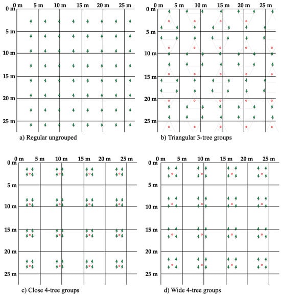
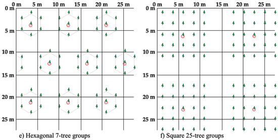
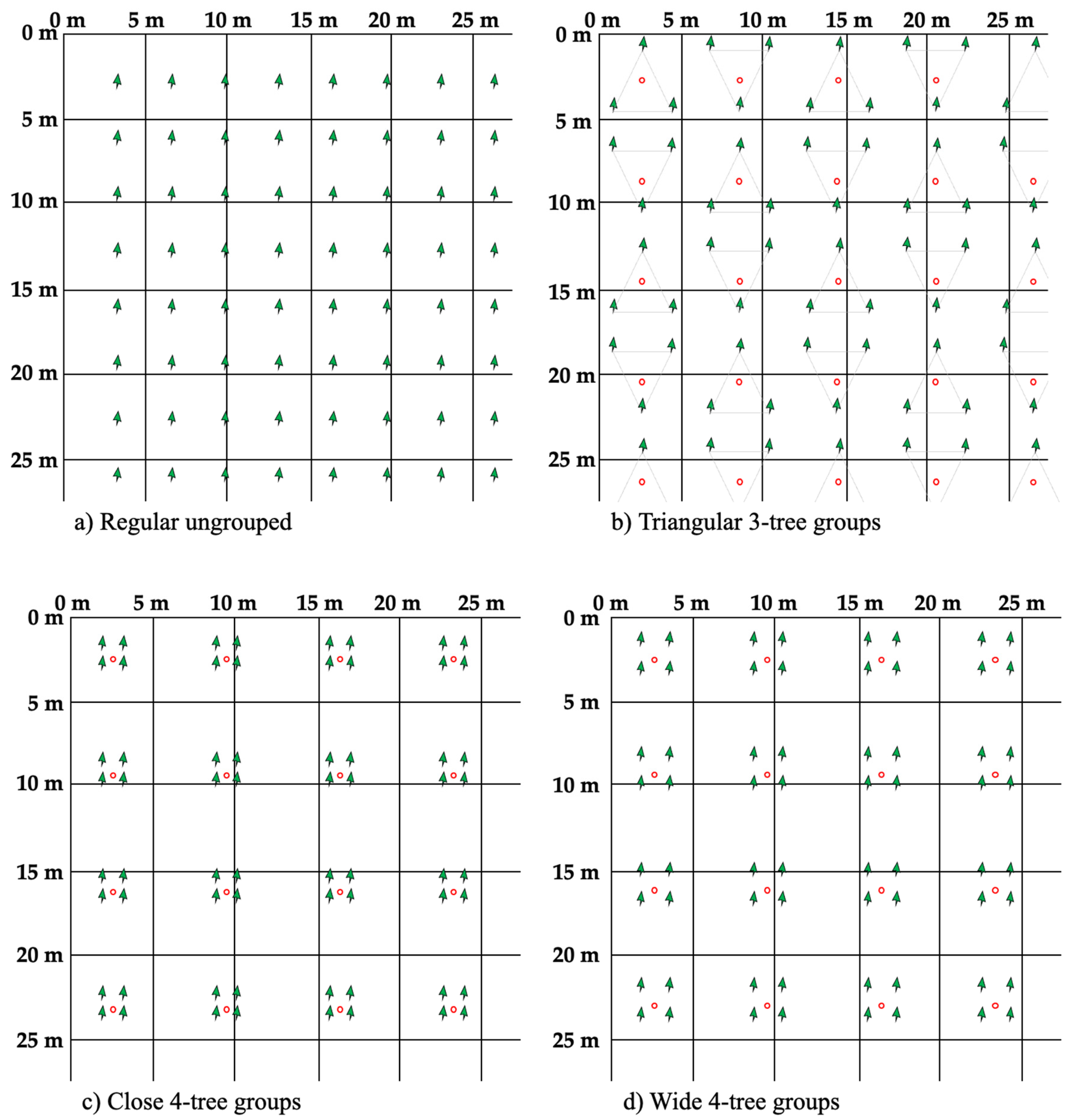
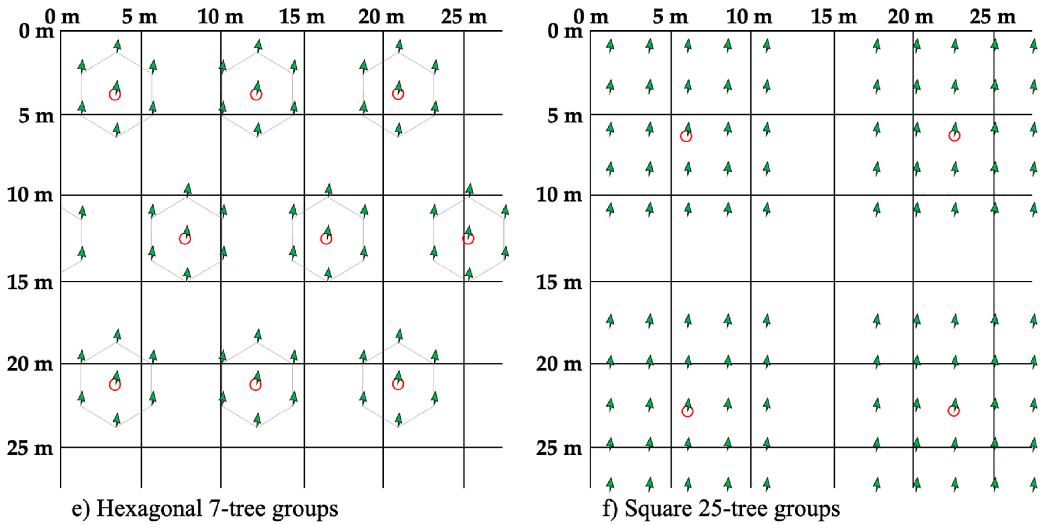
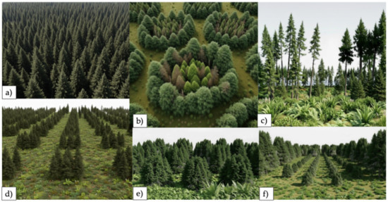
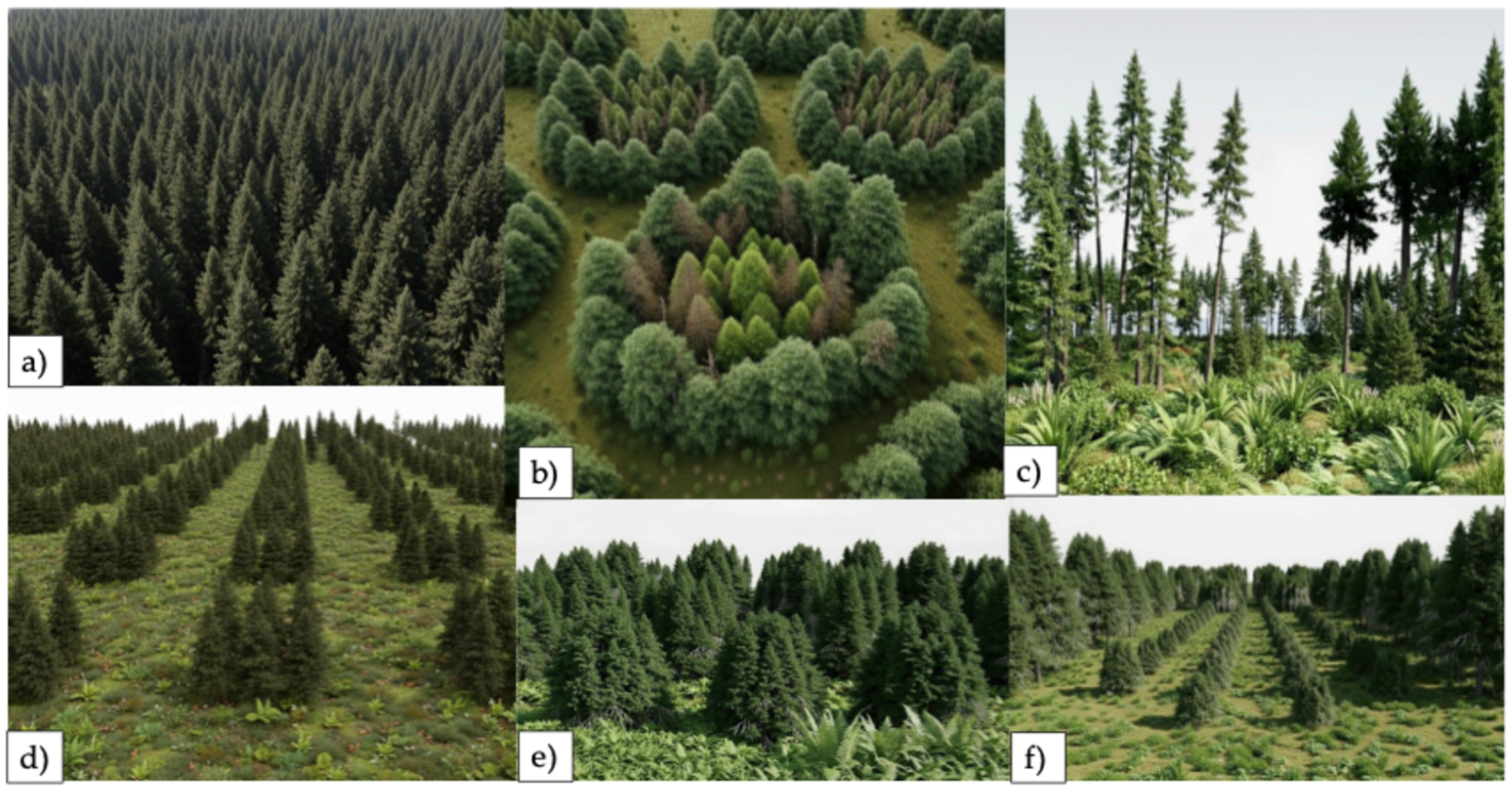
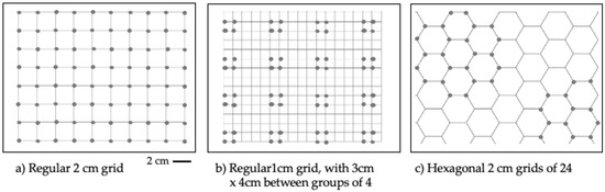
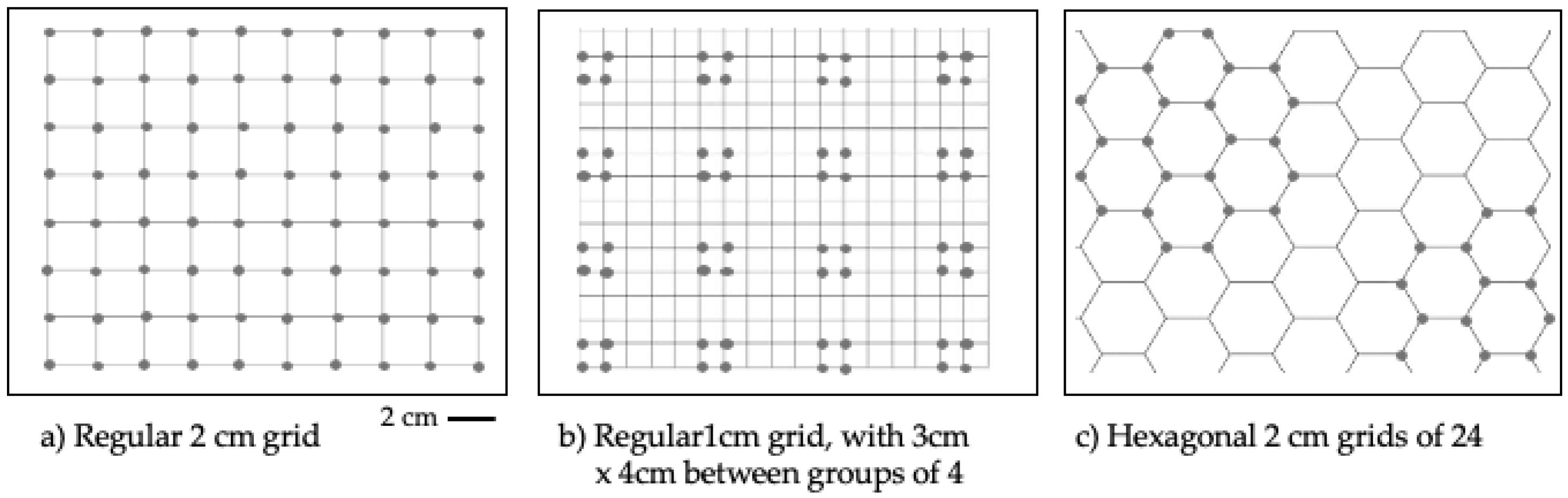
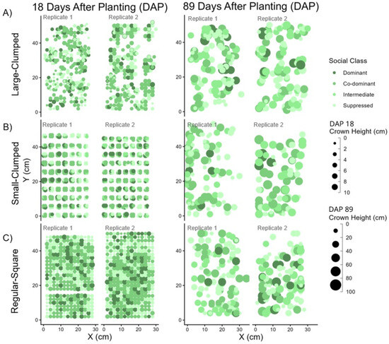
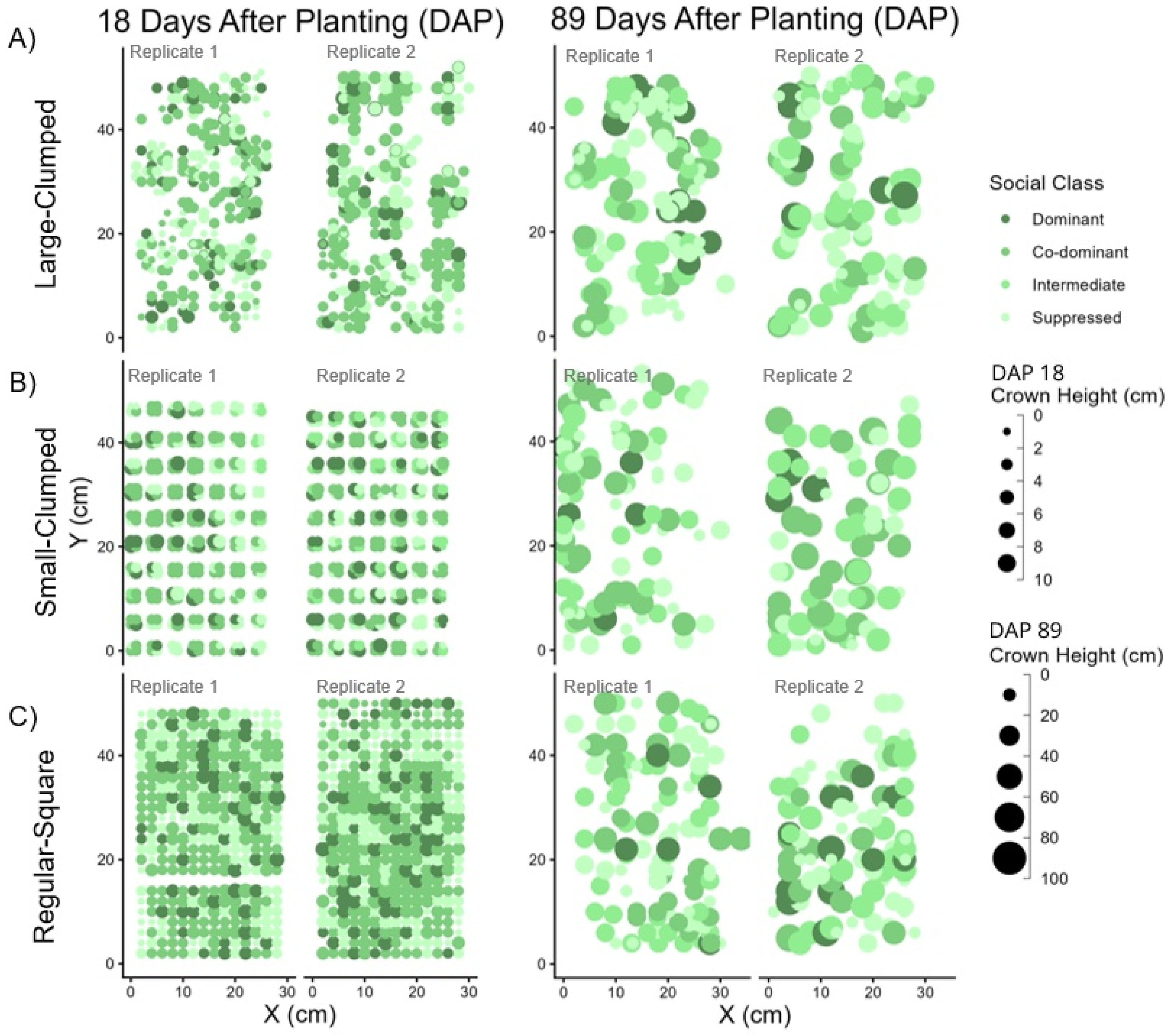
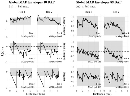
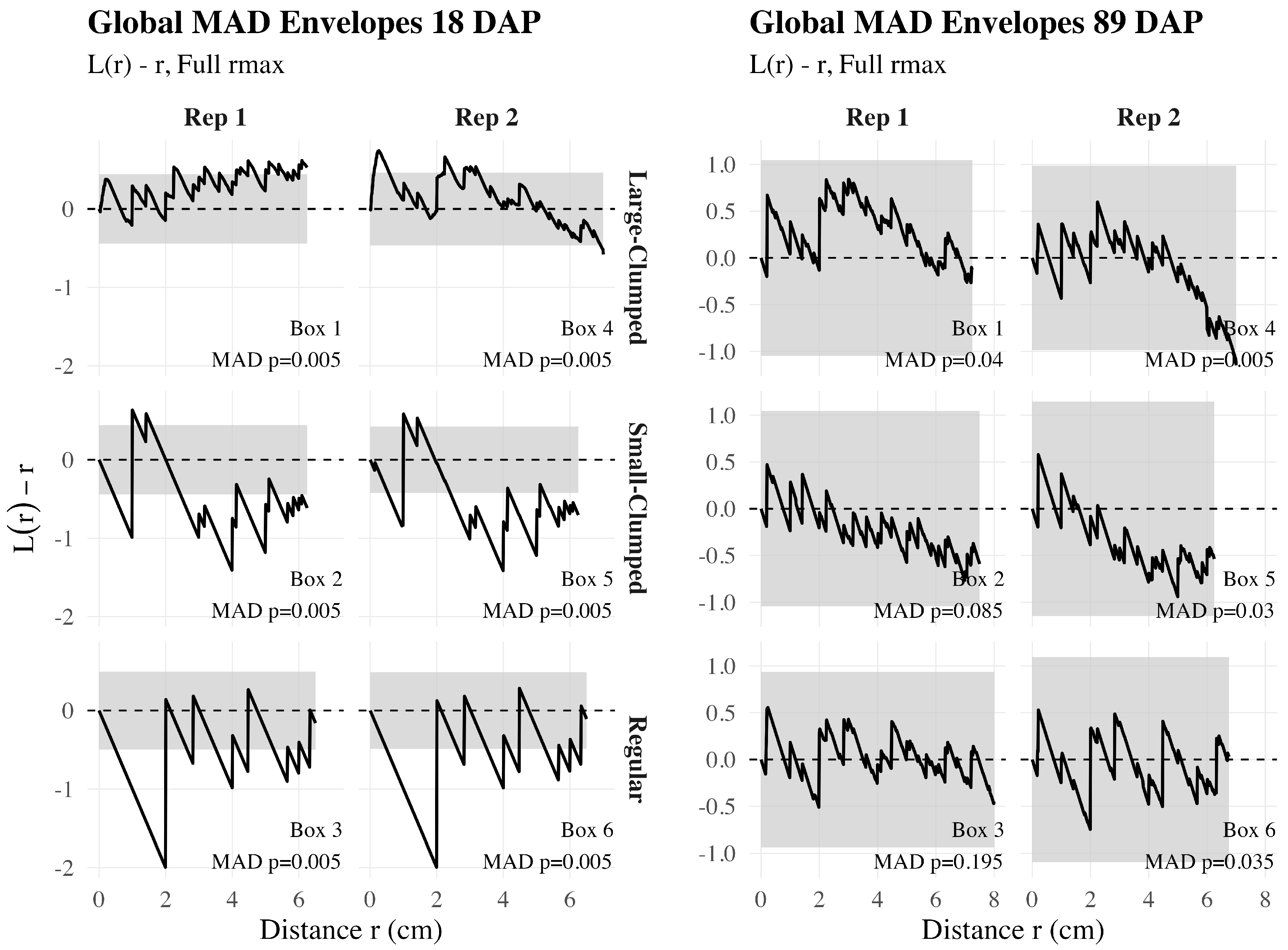

Disclaimer/Publisher’s Note: The statements, opinions and data contained in all publications are solely those of the individual author(s) and contributor(s) and not of MDPI and/or the editor(s). MDPI and/or the editor(s) disclaim responsibility for any injury to people or property resulting from any ideas, methods, instructions or products referred to in the content. |
© 2026 by the authors. Licensee MDPI, Basel, Switzerland. This article is an open access article distributed under the terms and conditions of the Creative Commons Attribution (CC BY) license.