


Abstract
Timber price dynamics are most often analysed using trends, seasonality, and classical measures of volatility, which describe the magnitude of fluctuations but only to a limited extent capture the temporal structure of the price-generating process. The aim of this study is to identify the structural complexity and long-term memory of quarterly prices of WC0 pine timber in the regional timber market in Poland. The analysis is based on nominal net prices (PLN/m3) from 16 forest districts of the Regional Directorate of State Forests in Kraków over the period 2005–2024, with reference to nationally averaged timber prices. Long-term dependence is assessed using the Hurst exponent estimated by detrended fluctuation analysis (DFA) applied to log returns, while the geometric complexity of price trajectories is characterised by the fractal dimension and additionally validated using the Higuchi estimator. Cross-sectional results reveal substantial spatial heterogeneity in scaling properties, indicating the coexistence of persistent (trend-following) and corrective (anti-persistent) dynamics across forest districts. Rolling-window analysis (40 quarters) demonstrates temporal variability in price dynamics, with particularly pronounced shifts observed in 2019–2021. Cluster analysis based on time-varying Hurst exponent values identifies two groups of forest districts with distinct persistence trajectories, corresponding to more trend-dominated and corrective price dynamics. In contrast, national-level prices generally exhibit higher persistence than local prices, reflecting the effects of price aggregation. Overall, the results show that fractal analysis uncovers persistent spatial and temporal differences in timber price structures that remain invisible when relying solely on variance-based measures, with direct implications for the choice of planning horizons and timber sale strategies in regional markets.
1. Introduction
Timber prices constitute one of the key elements of forest market functioning, influencing both economic decisions taken by forest resource management units and the profitability of investments in the forest-based sector. The existing literature is dominated by analyses focusing on price levels, long-term trends, seasonality, and classical measures of volatility, often based on time-series decomposition and econometric models [1,2,3,4,5]. At the same time, increasing attention is paid to the effects of macroeconomic factors, market globalisation, demand and supply shocks, and extraordinary events such as the COVID-19 pandemic or climate-related disturbances on the dynamics of wood product prices [6,7,8,9]. While these approaches provide important information on the magnitude and direction of price changes, they offer limited insight into the temporal structure of the price formation process, including the presence of long-term memory, the degree of order in price movements, and the irregularity of price trajectories.
Classical timber price forecasting models, such as ARIMA, SARIMA, structural models, and approaches based on artificial neural networks, primarily focus on minimising prediction errors over a given forecast horizon [2,5,10,11,12,13,14]. Although these methods are useful for short-term forecasting, they are not designed to directly assess long-term memory or scaling properties across different time horizons [5,7,15]. From the perspective of forest management these properties are of key importance, as they determine the level of variability, the nature of price risk, the persistence of market shocks, and the horizon over which sale decisions remain effective [2,6,16,17].
An important, though still relatively underutilised, analytical stream in forest research is represented by methods derived from fractal theory. Studies on timber prices rarely employ the concept of fractal dimension explicitly; instead, they often rely on closely related parameters, most notably the Hurst exponent and fractional Brownian motion models. For eucalyptus and pine timber prices, empirical evidence has demonstrated the presence of genuine long-range dependence in the price process and a superior performance of fractional models compared to standard geometric Brownian motion, both in terms of statistical properties and economic interpretation [18,19]. These findings suggest that the fractal structure of timber price dynamics may represent a persistent feature of timber markets, although its intensity may vary across markets, assortments, and institutional settings.
In parallel, an extensive body of financial literature is devoted to the analysis of fractal properties of price time series. Asset prices may exhibit self-similarity, long-term memory, and time-varying “roughness” of trajectories, leading to deviations from classical assumptions of market efficiency [20,21,22,23,24,25,26]. In this framework, the fractal dimension of a time trajectory serves as a measure of the geometric complexity of the process and, for one-dimensional time series, takes values between 1 and 2, with higher values corresponding to more irregular and random price behaviour [23,27]. Reviews of fractal dimension estimation methods emphasise the need to test the robustness of results with respect to sample length, non-stationarity, and noise, which is particularly relevant in economic data analysis [28,29]. Research on financial markets shows that the fractal dimension and closely related measures, such as the Hurst exponent and Hölder exponents, can be used to test the fractal nature of markets, identify deviations from efficiency, and analyse changes in underlying market mechanisms [29,30]. The usefulness of the Higuchi fractal dimension has also been demonstrated in the analysis of stock market indices [25,30] and in the modelling of financial instruments, where changes in the fractal dimension significantly affect the valuation of options and bonds in fractal frameworks [21,28,29,30]. These results suggest that the fractal dimension can be interpreted as a measure of structural complexity—and potentially risk—of the price process, independent of classical volatility-based measures.
Fractal measures, such as the Hurst exponent and the derived fractal dimension, directly address these issues by enabling a quantitative assessment of long-term memory in the price process and the geometric complexity of price trajectories over time [5,18,22,24]. In contrast to classical variance-based measures, which describe only the amplitude of fluctuations, fractal analysis captures the temporal organisation of price changes—specifically, whether price shocks are persistent or transitory, and whether price dynamics are relatively smooth or highly irregular [22,23]. Evidence from commodity and forest markets indicates that the dissipation of price shocks may extend over many years, with its pace depending on market structure, supply and demand conditions, as well as institutional and spatial factors [5,16,17].
The application of fractal analysis to timber prices should therefore be viewed as a complement, rather than an alternative, to classical forecasting methods. It extends timber market analysis beyond price levels and volatility, providing insight into the stability of the price process and the time variability of its structural properties. This is particularly relevant under conditions of increasing macroeconomic uncertainty, climate and energy pressures, and the growing complexity of price formation mechanisms in the forest-based sector [6,7,8,9,19,25]. In this context, fractal analysis can serve as a useful tool supporting both academic research and practical timber sales management. In recent years, the European timber market has operated under increasing structural pressure associated with the energy transition, the development of the bioeconomy, and the implementation of the European Green Deal. Growing demand for wood as a renewable energy source and as a low-carbon material, combined with episodic supply-side shocks—such as the COVID-19 pandemic, the energy crisis, and disruptions in global supply chains—has intensified the debate on the stability and predictability of timber markets within the European Union. In this context, assessing market stability requires not only measuring the magnitude of price volatility but also analysing the structural organisation of price movements over time.
In the forest economics literature, the Hurst exponent has been used only sporadically to assess long-term price memory, mainly in the calibration of fractional Brownian motion models [18,19]. By contrast, systematic analysis of the fractal dimension of timber price trajectories—treated as a measure of the degree of order, irregularity, and complexity of price movements over time—remains largely absent, particularly in a spatial framework at the forest district level. As a result, studies enabling an assessment of the structural properties of timber price dynamics comparable to that found in the financial literature, extending beyond classical indicators of price levels and volatility, are still lacking. The application of fractal analysis in the present study addresses this gap by enabling the identification of significant structural differences in the dynamics of WC0 timber prices across organisational units engaged in timber sales, which are not detectable using standard analytical tools.
Fractal properties, such as the Hurst exponent and the fractal dimension, allow for the evaluation of whether price impulses are persistent (trend-reinforcing) or anti-persistent (mean-reverting and rapidly dissipating). These measures can therefore be interpreted in economic terms—as indicators of price signal inertia, the degree of market integration, and the resilience of markets to shocks. From this perspective, fractal analysis complements classical volatility measures and contributes to the broader debate on the functioning of commodity markets under conditions of climate transition, regulatory transformation, and heightened macroeconomic uncertainty.
From the perspective of timber sales policy, the relevance of these results lies in a better understanding of the market conditions under which sales decisions are made. Knowledge of whether prices in a given unit exhibit ordered dynamics with long-term memory, or frequent directional changes with no stable structure, can support decisions regarding sales timing, planning horizons, and responses to periods of heightened market uncertainty. Consequently, fractal analysis constitutes a valuable complement to classical timber market analyses, enhancing their practical applicability.
The aim of this study is to identify and compare spatial and temporal differences in the complexity of quarterly WC0 pine timber prices across forest districts of the Regional Directorate of State Forests in Kraków over the period 2005–2024 using fractal analysis. Specifically, the study seeks to:
- estimate the fractal dimension as a measure of price path irregularity for each forest district;
- assess temporal changes in this measure using a rolling-window approach to detect transitions between periods of relative stability and increased complexity;
- identify groups of forest districts with similar fractal profiles, allowing for an assessment of the degree of commonality and/or locality in price formation mechanisms within the study region;
- compare the obtained results with those at the national (State Forests) levels.
2. Materials and Methods
2.1. Data Description
The study uses data on nominal quarterly net timber prices (PLN/m3) recorded over the period 2005–2024 in 16 forest districts of the Regional Directorate of State Forests in Kraków (RDSF Kraków). In addition, analyses include quarterly average timber prices obtained at the national level from the State Forests National Forest Holding (PGL LP).
Prices were neither deflated nor converted into a foreign currency (EUR) in order to avoid introducing additional transformations that could distort scaling properties and the potential fractal structure of the analysed time series.
The subject of the analysis is large-sized Scots pine timber of general purpose (WC0)—a roundwood assortment classified in the Polish timber grading system as raw material primarily intended for sawmill processing. During the analysed period, this assortment constituted the primary and strategically important commercial timber category in the region. Despite the relatively lower share of pine in the species composition of the Regional Directorate of State Forests in Kraków (RDSF Kraków) compared with the national average, this assortment was harvested in all analysed forest districts and remained subject to regular market transactions. This ensured the continuity and comparability of observations over time.
The spatial scope of the study covers 16 forest districts within RDSF Kraków. The choice of this area is motivated by both natural and organisational conditions, including substantial spatial heterogeneity and variation in the size of organisational units. These factors may lead to differences in production and economic conditions across forest districts, thereby affecting local price formation mechanisms. RDSF Kraków therefore provides a suitable case for analysing the dynamics of WC0 pine timber prices under conditions of spatial heterogeneity.
For each forest district, a time series of 80 quarterly observations (20 years × 4 quarters) is available. Given the relatively short length of individual series (N ≈ 80), the analytical methods were selected to be appropriate for short time series, for which classical econometric models may be less stable or require strong assumptions. In particular, the study employs fractal measures and rolling-window analyses, which allow the structure of price changes and its temporal variability to be examined without imposing a specific data-generating model.
Due to the limited length of the time series, fractal analysis methods recommended for short time series were applied [31].
2.2. Transformations
The analysis of the dynamic properties of timber prices was conducted using logarithmic price increments (log returns). The starting point was the price series Pt observed in consecutive quarters. For each forest district, price logarithms were computed as:
Then, log-returns were determined as the differences in subsequent price logarithms:
The use of logarithmic price increments is standard practice in the analysis of price time series, as it reduces the influence of price scale on the results, allows changes to be interpreted in relative rather than absolute terms, and often yields series with more stable statistical properties than those based on price levels [32]. Approximately, the log return rt can be interpreted as the quarterly rate of return (percentage price change) for a given forest district.
All measures applied in subsequent analyses were computed using these log returns. In particular:
- The standard deviation of log returns (ret_std) was treated as a classical measure of volatility [33];
- The Hurst exponent (H) was estimated using detrended fluctuation analysis (DFA) to assess persistence or anti-persistence in price changes [34];
- The fractal dimension (FD) was derived from the relationship FD = 2 − H and additionally validated using an independent estimator (the Higuchi method) [30,35].
In the dynamic analysis, a rolling-window approach was also employed, whereby measures such as H and FD were calculated over fixed-length data segments shifted through time. This approach allows assessment of whether the properties of price dynamics remain stable over the entire study period or vary across subperiods.
2.3. Methods
2.3.1. Hurst Exponent Estimated Using DFA
To assess long-term dependence properties in the analysed series, the Hurst exponent was estimated using detrended fluctuation analysis (DFA). DFA is widely applied in the analysis of short and potentially non-stationary time series [31], as it enables the investigation of scaling behaviour of fluctuations after removing deterministic trends within local segments of the data. As a result, the estimated Hurst exponent is less affected by trends and level shifts, which frequently occur in economic time series.
The analysis was conducted on logarithmic price increments (log returns) rt, as defined in Equation (2). For each forest district, log returns were treated as the primary input series for DFA computations. Since DFA is applied to logarithmic returns rather than price levels, the benchmark value corresponding to a random walk equals H = 0.5. In the first step, the so-called profile of the series (cumulative deviations from the mean) was constructed:
where denotes the mean value of log returns in a given series. The profile Y(k) was then divided into non-overlapping segments (windows) of length s. Within each segment, a trend was fitted (a linear trend in this study), and deviations of the profile from the fitted trend were computed. For a given scale s, the fluctuation function F(s) was calculated as the square root of the mean squared fitting error across all segments. The entire procedure was repeated for multiple values of s, corresponding to different time scales. If the series exhibits scaling behaviour, the following relationship holds:
F(s) ∝ sH
The Hurst exponent was estimated as the slope of the regression line in a log–log plot of (F(s)) against log(s).
The interpretation of the Hurst exponent in the context of price changes is as follows:
H > 0.5—persistence (trend-following behaviour): positive (negative) changes tend to be followed by changes of the same sign, indicating the presence of long-term positive dependence over time;
H ≈ 0.5—absence of long-term memory: behaviour close to a random process in which successive changes are approximately independent;
H < 0.5—anti-persistence (mean reversion): changes are more likely to reverse, indicating the dominance of corrective mechanisms and more frequent directional shifts [36].
In the subsequent analysis, H values were estimated both for the entire available sample for each forest district and within a dynamic framework using rolling windows. This allows assessment of whether persistence or anti-persistence properties remain stable over time or vary across successive subperiods.
2.3.2. Fractal Dimension Derived from the Relationship
To complement the interpretation of the results obtained for the Hurst exponent, the concept of the fractal dimension of the time series graph was employed. The fractal dimension serves as a measure of the geometric complexity of a time trajectory and is often interpreted as an indicator of its “roughness” (irregularity) [37]. In the context of time series, the more jagged and irregular the evolution of values over time, the higher the fractal dimension of the graph; conversely, smoother trajectories dominated by trends correspond to lower FD values.
In the literature on self-similar processes and time series with fractal properties, the relationship linking the Hurst exponent H to the fractal dimension of the time series graph (for a one-dimensional temporal trajectory) is commonly expressed as [38]:
FD= 2 − H
In this study, FD values were calculated using the above relationship, based on H estimates obtained via DFA applied to log returns. This relationship allows a transition from a strictly temporal interpretation (process memory, persistence/anti-persistence) to a geometric one: an increase in H implies stronger persistence and simultaneously lower trajectory irregularity (lower FD), whereas a decrease in H indicates a dominance of corrective mechanisms and more frequent directional changes, which translates into greater jaggedness of the graph (higher FD).
For practical interpretation, a convenient reference point is FD = 1.5, corresponding to H = 0.5.
Specifically:
FD < 1.5—the trajectory is relatively smoother and changes exhibit persistence, corresponding to a more trend-dominated dynamic;
FD ≈ 1.5—behaviour close to random, with no pronounced long-term memory;
FD > 1.5—the trajectory is more irregular and rougher with more frequent reversals, corresponding to anti-persistence (dominance of corrective mechanisms) [39].
In subsequent analyses, the fractal dimension FD was used for cross-district comparisons and for assessing temporal changes in dynamic properties using rolling-window analysis, treating it as a complementary geometric measure of the complexity of price paths.
2.3.3. Rolling-Window Analysis
To capture changes in the dynamic properties of timber prices over time, a rolling-window analysis was applied. This approach is particularly useful for economic data, for which the assumption of constant parameters over the entire study period is often too restrictive. In addition to estimating a single Hurst exponent value for the full period 2005–2024, the exponent was repeatedly calculated over successive, overlapping data segments, allowing the identification of periods with differing price dynamics (so-called regimes).
A window length of 40 quarters (40Q), corresponding to a 10-year horizon, was adopted. The window was shifted forward by one quarter at a time, yielding a time series of rolling estimates. Formally, for each log-return series the rt sub-sequences, rt−39, rt−38, …, rt, were considered for successive values of t, starting from the point at which at least 40 observations were available. For each window, the Hurst exponent was estimated using DFA, resulting in a rolling series H_roll_40Q(t). The corresponding rolling fractal dimension was then computed.
The choice of a 40Q window represents a compromise between estimation stability and the ability to observe temporal changes. On the one hand, a 10-year window provides a sufficient number of observations for relatively stable estimation of H using DFA; on the other hand, shifting the window quarterly allows the evolution of market dynamics to be tracked across successive subperiods. In practice, the resulting series H_roll_40Q(t), were interpreted as time-varying measures of persistence and irregularity in price changes.
The aim of the rolling-window analysis was to identify changes in the nature of price formation over time, interpreted as periods characterised by different memory structures and degrees of price irregularity. In particular:
- An increase in H_roll_40Q(t) above 0.5 indicates stronger persistence (a more trend-dominated character of changes) within a given 10-year horizon;
- A decrease in H_roll_40Q(t) below 0.5 suggests anti-persistence and more frequent corrections (mean reversion).
The results of the rolling-window analysis were subsequently used for comparisons across forest districts and to assess whether the observed fractal properties remain stable over time or undergo significant changes across different phases of the study period.
2.3.4. Robustness to Window Length
Since the rolling DFA requires specifying a window length, we examine whether the results depend on this choice. In the baseline specification the rolling DFA is computed using a window of 40 observations. To assess robustness, the analysis was repeated for alternative window lengths W = 32, 36, 40, 44, and 48.
2.3.5. Validation: Higuchi Fractal Dimension
To enhance the robustness of the conclusions and to verify whether the observed differences across forest districts are not solely an artefact of the chosen method for estimating the Hurst exponent, a validation exercise was conducted using an independent, direct estimator of fractal dimension—the Higuchi method (Higuchi FD) [30].
The Higuchi method estimates the fractal dimension directly from the time series by analysing the length of the trajectory across different discretisation scales. Unlike the FD = 2 − H approach, which is based on a theoretical relationship between process parameters, the Higuchi FD is a purely geometric measure derived without reference to the Hurst exponent. As such, it can serve as a consistency check (validation tool) for the results: if both approaches lead to similar conclusions—for example, comparable rankings of forest districts—this strengthens the interpretation that the observed heterogeneity reflects genuine properties of the data rather than artefacts of a particular estimator. Consistent with the rest of the methodology, the Higuchi FD was computed using log returns for each forest district.
2.3.6. Cluster Analysis (Ward’s Method with Euclidean Distance)
To identify groups of forest districts exhibiting similar dynamics of price changes over time, hierarchical cluster analysis was applied [40]. The basis for clustering consisted of the time profiles of the Hurst exponent, that is, the values H_roll_40Q(t). For each forest district, a vector of successive Hurst exponent values was constructed and treated as a set of features describing the evolution of dynamic properties over time.
Ward’s method with Euclidean distance was employed [41]. Ward’s method is an agglomerative clustering approach in which, at each step, the two clusters whose merger results in the smallest increase in within-cluster variance are combined. This procedure favours the formation of relatively homogeneous clusters.
2.4. Study Area
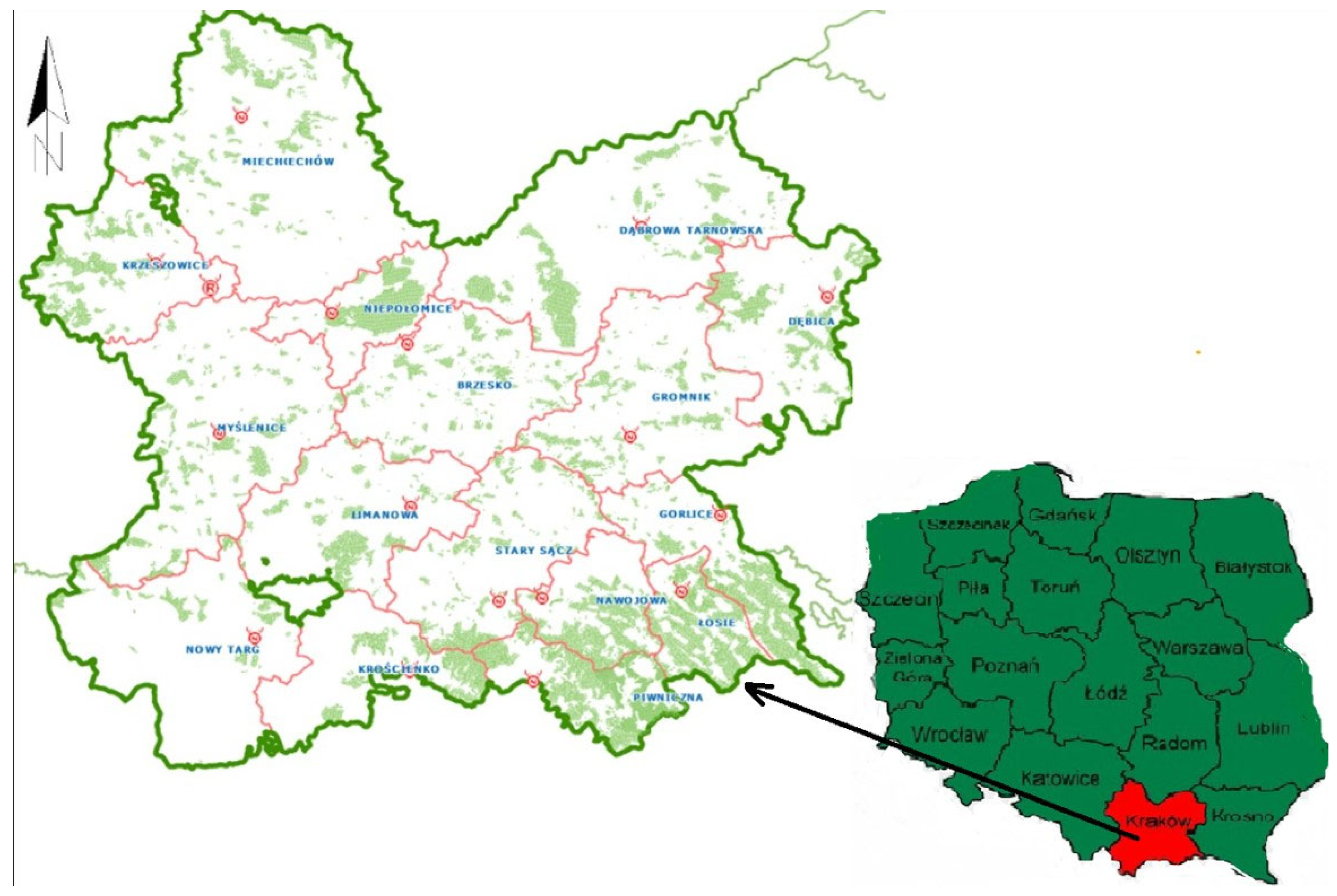
Forests managed by the Regional Directorate of State Forests in Kraków are state-owned and form part of the Polish State Forests National Forest Holding. In Poland, state-owned forests account for approximately 77% of total forest area, which makes the institutional framework of public forest management highly relevant for timber market functioning at the national level. In 2024, the State Forests National Forest Holding sold approximately 40.6 million m3 of timber, which underscores the macroeconomic importance of this institutional framework for the national wood market. The predominance of public ownership may influence market characteristics, including the organisation of timber sales and price formation mechanisms. Therefore, the findings should be interpreted primarily within the context of markets operating under centralised, state-managed forest ownership structures. The study was conducted in forest districts administratively subordinate to the Regional Directorate of State Forests in Kraków (RDSF Kraków). RDSF Kraków is the smallest of the 17 organisational units of the State Forests National Forest Holding. The total area under its management amounts to 173.6 thousand hectares, including 171.1 thousand hectares of forest land. Forest cover (forest cover rate) in the area administered by RDSF Kraków amounts to approximately 30.8%, which is close to the national average and reflects the mixed mountainous–upland character of the region. RDSF Kraków is divided into sixteen forest districts (Figure 1). The area of State Treasury forests ranges from 5.2 thousand hectares in the Nowy Targ Forest District to 16.9 thousand hectares in the Łosie Forest District. The average forest district area is 10.8 thousand hectares, which is among the smallest within the State Forests system [42]. The largest territorial extent is observed in the Miechów and Dąbrowa Tarnowska Forest Districts, while the smallest administrative areas are found in the Niepołomice and Piwniczna Forest Districts.
The analysed Directorate is characterised by considerable terrain heterogeneity. Mountain habitats dominate, accounting for 54% of the area, followed by upland habitats (24%), while lowland habitats cover 22%. Coniferous species prevail in the species composition, occupying 62% of the forest area, including pine (31%) and fir (23%). The share of pine has been systematically declining, particularly in mountain forest districts. Broadleaved species account for 38% of the area [43]. In terms of age structure, stands aged 61–100 years (age classes IV and V) dominate, covering 23.3% and 16.2% of the area, respectively. A substantial share (22.6%) is occupied by stands in the regeneration class (RC), defined as mature stands with a developing younger generation.
Timber harvesting in RDSF Kraków in 2024 amounted to 973.4 thousand m3, including 581.1 thousand m3 of coniferous timber (of which 408 thousand m3 was large-size timber) and 373 thousand m3 of broadleaved timber (including 170 thousand m3 of large-size assortments). The average timber price achieved in the State Forests in 2024 was PLN 276.35 per m3, while in RDSF Kraków it reached PLN 302.32 per m3, placing this Directorate among the top units nationwide in terms of achieved timber prices [42].
Figure 1.
Location of the forest districts of the Regional Directorate of State Forests in Kraków—indicative map (red color—RDLP Kraków on the map of Poland, the arrow—indicates the division of RDLP Kraków into forest districts). Source: https://www.krakow.lasy.gov.pl/o-dyrekcji (accessed on 25 January 2026) [44]. https://pl.wikipedia.org/wiki/Plik:RDLP_Krak%C3%B3w.svg (accessed on 25 January 2026) [45].
3. Results
3.1. Price Levels and Variability of Timber Prices in Forest Districts of RDSF Kraków
Over the period 2005–2024, average timber prices in the analysed forest districts ranged approximately from PLN 249 to PLN 279 per m3. Differences are evident in maximum price levels—reaching up to PLN 550 per m3 in the Nowy Targ Forest District—as well as in standard deviation (SD), indicating heterogeneous magnitudes of price fluctuations across individual units. The highest price volatility is observed in forest districts such as Nowy Targ, Piwniczna, and Stary Sącz. In contrast, prices in the Łosie and Gorlice Forest Districts were the most stable during the study period (Table 1).
Table 1.
Summary statistics of WC0 pine timber prices in forest districts of RDSF Kraków (2005–2024).
3.2. Fractal Measures and Cross-Sectional Timber Price Volatility
Table 2 presents the Hurst exponent on log returns, the corresponding fractal dimension, and the standard deviation of log returns (ret_std) as a classical measure of volatility (Table 2). The range of H values (0.39–0.67) indicates substantial heterogeneity in long-memory properties and in the degree of irregularity of price trajectories across forest districts. The juxtaposition of fractal measures with classical volatility (ret_std) suggests that timber price dynamics are complex and cannot be fully characterised using variance-based measures alone. The highest price uncertainty (risk), as reflected by ret_std, is observed in the Nowy Targ Forest District, whereas the most predictable prices occurred in the Miechów Forest District (Table 2).
Table 2.
Fractal measures and variability of log-returns of timber prices in forest districts (2005–2024).
To visualize and facilitate the comparison of forest districts in terms of the degree of irregularity of price dynamics, FD values were presented in the form of a ranking and graphically illustrated (Figure 2).
Figure 2.
Ranking of forest districts according to the FD fractal dimension determined on the log-returns of timber prices (2005–2024).
The vertical line denotes the reference value FD = 1.5, corresponding to H = 0.5. Forest districts with FD values above 1.5 exhibit greater “roughness” and irregularity in timber price changes, reflected in more frequent reversals in price movements. In contrast, FD values below 1.5 correspond to smoother trajectories and stronger persistence in timber price changes, indicating a more trend-dominated dynamic. The figure reveals pronounced heterogeneity across forest districts: the highest FD values (approximately 1.58–1.61) are observed in the Nawojowa and Krościenko Forest Districts, suggesting the most irregular, corrective price dynamics. Elevated FD values are also found in the Myślenice and Nowy Targ Forest Districts, indicating relatively frequent directional changes in price fluctuations. Conversely, the lowest FD values are recorded for the Miechów Forest District (approximately 1.33) and for districts located in the lower part of the ranking (including Dębica, Gorlice, Niepołomice, and Dąbrowa Tarnowska), which implies a more trend-oriented character of price changes and stronger persistence over the study period. The position of some forest districts close to the reference value FD = 1.5 (e.g., Gromnik and Brzesko) suggests dynamics close to random behaviour, with no clear dominance of either trend-following or corrective mechanisms. Overall, the ranking confirms that the structure of timber price changes varies spatially, and that the fractal measure provides a useful ordering of forest districts in terms of the degree of irregularity and process memory.
3.2.1. Validation of Fractal Measures Using the Higuchi Estimator
Validation was conducted by analysing the relationship between the fractal dimension estimated using the Higuchi method and the fractal dimension derived indirectly from the Hurst exponent estimated via DFA. This relationship is presented in the form of a scatter plot and was quantified using a correlation coefficient (Figure 3). The distribution of points exhibits an upward-sloping pattern, indicating consistency between the measures. At the same time, some dispersion is expected, as the estimators differ in their statistical properties and sensitivity to noise, and the length of the time series is limited (N ≈ 80).
Figure 3.
Relationship between Higuchi FD and FD: each point corresponds to a forest district and compares the fractal dimension obtained from DFA with the Higuchi fractal dimension estimated directly from the log-return series.
The results indicate a positive relationship between the two estimators, confirming the consistency of conclusions regarding the relative roughness of the analysed price series. At the same time, the observed dispersion of points reflects differences in the statistical properties of the estimators as well as the limited length of the time series. The application of the independent Higuchi estimator confirmed the overall consistency of the fractal analysis results obtained using the DFA method, thereby strengthening the credibility of the empirical findings. The correlation between the estimators equals 0.65, indicating a moderately strong agreement in the rankings of the analysed series. This result confirms that both approaches identify similar differences in the structure of timber price dynamics, despite differences in estimator properties and the limited length of the time series.
3.2.2. Diagnostic Tests for the Hurst Exponent Estimates
Since some estimated Hurst exponent values fall below the benchmark H = 0.5, additional diagnostic tests were performed to verify whether these results may arise from estimator bias, finite-sample effects, or methodological choices in the DFA procedure. First, a calibration test was conducted using Gaussian white noise with the same sample length (T = 80) and identical DFA settings (same detrending order and the same set of scales: [4,5,7,10,14,20,28,39]). For this benchmark process, the estimated value was H = 0.5004, which is consistent with the theoretical expectation H = 0.5 for a memory-less process. This confirms that the estimator does not exhibit a downward bias under the adopted configuration.
Second, a permutation test was performed by randomly shuffling the temporal order of returns while preserving their marginal distribution. This procedure destroys temporal dependence but leaves the unconditional distribution unchanged. After permutation, the mean estimated value increased from H ≈ 0.128 in the original data to H ≈ 0.541. The substantial increase indicates that the low H observed in the empirical series is driven by temporal structure rather than by the distribution of returns.
Taken together, these results suggest that the low values of H observed in the empirical data reflect genuine anti-persistent (mean-reverting) scaling behaviour within the analysed range of scales rather than artefacts of the estimation procedure or the relatively short sample length.
3.2.3. Results of the Window Length Robustness Test
Figure 4 presents the mean rolling Hurst exponent H roll, W(t) obtained for the different window sizes. The resulting curves display very similar dynamics across all window lengths and largely overlap throughout the sample period. Moreover, the estimated values remain within a comparable range across all specifications.
Figure 4.
Robustness of rolling DFA estimates to window length.
This indicates that the rolling DFA results are not sensitive to the particular choice of the window length and that the observed patterns represent stable properties of the analysed series rather than artefacts of the rolling window specification.
3.3. Temporal Variability of Fractal Properties—Rolling-Window Analysis
Figure 5 illustrates the evolution over time of the average Hurst exponent, calculated using 10-year rolling windows and averaged across all forest districts. Since each value of H_roll_40Q(t) reflects the dynamic properties of price movements over the preceding decade, the trajectory of the curve should be interpreted as the evolution of market phases across successive subperiods, characterised by differing degrees of persistence and irregularity in price dynamics.
Figure 5.
Average Hurst exponent estimated using 40-quarter (10-year) rolling windows, averaged across forest districts. The horizontal line denotes the threshold H = 0.5.
During the period 2015–2018, the Hurst exponent remained clearly above 0.5 (approximately 0.62–0.73), indicating a dominance of persistence and a more trend-driven character of price dynamics within the 10-year rolling windows. In contrast, during 2019–2021, a decline in H below the 0.5 threshold was observed (with a minimum of approximately 0.44–0.45), signalling a transition to anti-persistent dynamics, characterised by a predominance of corrective mechanisms and more frequent reversals in price movements within the analysed windows. This was followed by a short-term increase in H in 2022, a renewed decline in 2023, and a pronounced increase in 2024–2025 (to approximately 0.77), indicating a return to strongly persistent, trend-dominated price dynamics. In summary, the trajectory of H_roll_40Q(t) demonstrates that the dynamic properties of timber prices are not constant over time: the market alternated between periods characterised by stronger persistence and periods dominated by corrective, anti-persistent behaviour. This provides justification for the use of rolling-window analysis and indicates the presence of time-varying phases in timber price dynamics.
3.4. Grouping of Forest Districts Based on Price Dynamics Properties
3.4.1. Identification of Clusters and Temporal Heterogeneity in Price Dynamics
The similarity of the H_roll_40Q(t) trajectories provides a basis for grouping forest districts using cluster analysis. The results of hierarchical clustering are presented in the form of a dendrogram (Figure 6), which was used to determine the appropriate number of clusters. In this study, due to a clear “cut-off” point in the dendrogram and the interpretability of the resulting groups, a two-cluster solution was adopted. Each forest district was subsequently assigned a cluster label, and the identified groups were further characterised using static measures (including the Hurst exponent H, fractal dimension FD and the volatility of log returns). This approach enabled the interpretation of clusters in terms of distinct patterns of timber price dynamics.
Figure 6.
Dendrogram of hierarchical clustering of forest districts based on H_roll_40Q(t).
To determine the appropriate number of clusters, we evaluated several candidate solutions using the silhouette coefficient. The analysis was performed for cluster numbers ranging from 2 to 5. The results indicate that the silhouette score reaches its maximum for the two-cluster solution (0.406), while substantially lower values are obtained for larger numbers of clusters (0.244 for k = 3, 0.180 for k = 4, and 0.148 for k = 5). This suggests that the two-cluster specification provides the most distinct separation between groups and therefore was adopted in the subsequent analysis.
Figure 7 presents the average time profiles of the Hurst exponent for the two clusters of forest districts identified on the basis of similarity in the H_roll_40Q(t) trajectories. The resulting clusters differ both in their levels and in their temporal behaviour, indicating the existence of two distinct types of timber price dynamics.
Figure 7.
Average trajectories of H_roll_40Q(t) for clusters identified using Ward’s hierarchical clustering method with Euclidean distance. The horizontal line denotes the threshold H = 0.5 (Cluster 1: Stary Sącz, Limanowa, Piwniczna, Myślenice, Nowy Targ, Krościenko; Cluster 2: Miechów, Dębica, Gorlice, Niepołomice, Dąbrowa Tarnowska, Łosie, Krzeszowice, Brzesko, Gromnik, Nawojowa).
Cluster 1 (n = 6) (blue line) exhibits markedly lower values of H_roll_40Q(t). In the initial period (2015–2018), values fluctuate around 0.50–0.58, i.e., close to the persistence threshold. From approximately 2019 onward, a decline below 0.5 is observed, with a pronounced minimum around 2020–2021 (approximately 0.32–0.40), indicating a dominance of anti-persistent dynamics and more frequent corrective price movements. During 2022–2023, values generally remain below 0.5, while in 2024–2025, a clear rebound towards and above 0.5 is evident, suggesting a potential shift in price dynamics in the most recent period. Cluster 2 (n = 10) (orange line in Figure 6) is characterised by consistently higher values of H_roll_40Q(t) throughout the analysed period. During 2015–2018, values range approximately from 0.65 to 0.82, indicating strong persistence and a more pronounced trend-following character of price changes within the 10-year windows. Around 2020–2021, a decline in H towards 0.5 is observed; however, this cluster largely remains within the persistence regime. In the final part of the series (2024–2025), a renewed and pronounced increase in H is observed, suggesting a return to a strongly trend-dominated character in the most recent 10-year windows.
In summary, cluster analysis based on H_roll_40Q(t) profiles identified two distinct groups of forest districts: (I) forest districts characterized by more corrective and irregular dynamics, with more frequent drops of H below 0.5, and (II) forest districts showing more trend-driven dynamics, which is reflected in consistently higher values of H. This result confirms that the heterogeneity of timber price dynamics is not limited to differences in the levels of static measures, but also to the temporal evolution of dynamic properties over time.
3.4.2. Characterisation of Clusters Using Static Measures and the Volatility Space
To interpret the identified clusters, forest districts were first assigned to clusters and then characterised using static measures calculated for the entire period 2005–2024 for H, FD, and ret_std (Table 3).
Table 3.
Descriptive statistics of fractal measures and volatility across clusters.
Figure 8 illustrates the position of forest districts in the space defined by two static measures: the persistence of price changes, measured by the Hurst exponent, and classical volatility of log returns. Points are coloured according to the clusters obtained from the similarity of the H_roll_40Q(t) trajectories over time, which allows assessment of whether groups identified on the basis of rolling profiles also differ with respect to global measures. The vertical axis represents H computed for the entire period 2005–2024, while the horizontal axis shows the standard deviation of log returns. Colours indicate cluster membership as determined by Ward’s method applied to the H_roll_40Q(t) profiles. The horizontal line denotes the threshold H = 0.5. A clear separation of clusters along the H axis is evident. Cluster 1 (blue) includes forest districts with H values below 0.5, indicating a predominance of anti-persistence, characterised by more frequent reversals in price movements and stronger corrective mechanisms. This group includes, among others, Piwniczna, Stary Sącz, Limanowa, Myślenice, Nowy Targ, and Krościenko. For some forest districts in Cluster 1, higher volatility is also observed (e.g., Nowy Targ and Krościenko), suggesting a combination of large fluctuation amplitudes with a corrective dynamic. Cluster 2 (orange) consists mainly of forest districts with H values above 0.5, indicating persistent, more trend-dominated price dynamics over the entire period. This group includes Miechów, Dębica, Gorlice, Niepołomice, Dąbrowa Tarnowska, Łosie, Krzeszowice, and Brzesko. Volatility in this cluster is generally low to moderate (approximately 0.06–0.09), suggesting relatively smaller quarterly price fluctuations compared with Cluster 1. Borderline cases are also noteworthy. Gromnik lies close to the H = 0.5 threshold, indicating dynamics close to random behaviour, while Nawojowa exhibits a low H value but is assigned to Cluster 2. This suggests that cluster membership is determined primarily by the shape of the H_roll_40Q(t) profile over time rather than by a single Hurst exponent value computed for the entire period. In summary, the figure confirms the interpretation of the clusters: the groups identified on the basis of H_roll_40Q(t) profiles differ not only in the temporal evolution of H but also in average persistence levels and, to some extent, in the volatility of log returns. This allows the clusters to be given an economic interpretation: Cluster 2 corresponds to forest districts with more trend-dominated price dynamics, whereas Cluster 1 represents districts characterised by more frequent corrections and greater irregularity in price movements.
Figure 8.
Forest districts grouped based on H_roll_40Q(t) profiles against the Hurst exponent for the entire period and log-return variability.
3.5. National Average Prices as a Benchmark for Price Dynamics
Data for the whole of Poland represent an aggregate (national average), which limits the scope for cross-sectional comparisons at the forest district level. In the analysis, the national series was used as a benchmark for the forest districts of RDSF Kraków by comparing fractal measures and their temporal variability (Figure 9). Given the relatively short window length (40 observations), DFA estimation may be sensitive to the choice of scales; therefore, a fixed set of scales limited to half the window length was applied, which stabilises the results and enables meaningful comparisons of price dynamics.
Figure 9.
Poland (So WC0): Hurst exponent H_roll_40Q(t) estimated in 40-quarter (10-year) windows with a constant set of scales. H values were calculated on quarterly log returns. The time axis refers to the end of the 10-year window.
The figure presents the trajectory of the Hurst exponent estimated using 40-quarter rolling windows for the reference time series—the national average WC0 price series. In contrast to earlier results, the application of a fixed set of scales in the DFA reduced estimation instability associated with the short window length, thereby allowing meaningful interpretation of temporal changes. During the period 2015–2019, values of H_roll_40Q(t) remained elevated (approximately 0.85–1.10), indicating a dominance of persistence over the long (10-year) horizon and a more trend-dominated character of national average price dynamics. Around 2020–2021, a pronounced decline in H to approximately 0.68–0.75 is observed, suggesting a weakening of trend-following behaviour and an increased role of corrective mechanisms in subsequent windows. The most substantial change in dynamic properties occurs around 2022/2023, when H drops sharply to values close to 0.5, corresponding to the boundary between random behaviour and the absence of long-term memory. This point represents a turning phase, after which values begin to increase again, and in 2023–2024 levels above approximately 0.6–0.9 once more dominate, indicating a return to more persistent dynamics. In the final segment (2024–2025), a very strong increase in H is observed; however, this should be interpreted with caution, as rolling-window estimates at the end of the sample may be more sensitive to isolated strong price episodes in recent years and to the limited sample length. Comparing the national results with those obtained for RDSF Kraków, the average H_roll_40Q(t) for the regional series was lower and more frequently declined towards or below 0.5 (particularly around 2020–2021), indicating periods in which corrective mechanisms temporarily dominated price dynamics.
4. Discussion
The results indicate substantial spatial heterogeneity in the structure of temporal dependence across forest districts within the RDSF Kraków. Although the estimated range of the Hurst exponent (H ≈ 0.39–0.67) should be interpreted comparatively rather than as precise point estimates due to the finite sample length (N ≈ 80), the relative differences between forest districts are economically meaningful. This implies that local timber markets differ markedly in the degree of persistence in price changes (H > 0.5) and in the prevalence of corrective, mean-reverting behaviour (H < 0.5). Such an interpretation is consistent with the theoretical foundations of DFA as a tool for detecting long-range dependence in potentially non-stationary time series, where classical variance-based measures do not distinguish the structure of price changes (memory, ordering) from their amplitude alone [46,47,48]. These findings should be read as evidence of heterogeneous temporal structure across sales units, rather than as a claim about the exact magnitude of persistence in any single district.
The joint consideration of fractal measures (H, FD) and classical volatility (ret_std) confirms that price risk has at least two complementary dimensions, the magnitude of fluctuations and their temporal organisation, which are related to process memory and the irregularity of price trajectories. This finding is consistent with recent literature on fractal analysis of commodity and financial markets, which demonstrates that scaling-based measures reveal information that remains hidden when using standard variance-based indicators [49,50]. In this framework, the fractal dimension can be interpreted as an independent descriptor of the price process, providing insight into the complexity of price dynamics [51]. Compared with previous studies documenting long-memory behaviour in forest product markets at national or aggregated levels the present results extend the literature by demonstrating that persistence structures may vary considerably within a single national system governed by uniform sales regulations. Thus, the Polish case both confirms the presence of long-memory behaviour identified in earlier studies and refines existing evidence by revealing substantial intra-national heterogeneity in scaling properties. Accordingly, the contribution of this study lies not in identifying volatility per se, but in distinguishing between markets where shocks tend to persist and those where they dissipate more rapidly. This nuance matters for interpretation: markets may exhibit similar volatility levels yet differ in how quickly price impulses decay, which affects the practical interpretation of risk in the context of planning horizons.
The inclusion of an independent fractal dimension estimator (Higuchi FD) further strengthens the interpretation of the results by allowing comparison between two conceptually distinct estimation approaches: (1) the indirect relationship FD = 2 − H, grounded in the theory of self-similar processes; (2) a purely geometric approach in which the fractal dimension is estimated directly from the time-series trajectory. The Higuchi method is a classical and widely used estimator of fractal dimension for discrete data and has been extensively applied to assess time-series complexity in natural sciences, medicine, and economics [30,52,53,54]. The observed moderately strong agreement between the estimators (correlation ≈ 0.65) should not be interpreted as numerical equivalence but rather as consistency in ranking relative roughness across districts. Given the relatively short time series, estimation errors may increase, and cross-validation using multiple estimators is recommended as good practice [55]. The validation applied in this study follows these recommendations, reducing the risk that the results reflect artefacts of a single estimation method. Therefore, the main value of the validation is methodological: it supports the stability of cross-district ordering in “roughness” rather than the exact point values of FD.
From the perspective of the RDSF Kraków region, which is characterised by heterogeneity in the size of managed units and habitat structure, the observed range of H and FD values may reflect differences in supply conditions, sensitivity to local logistical and demand constraints, and the extent to which prices are “smoothed” by sales mechanisms. Common institutional conditions and uniform timber sales rules across the State Forests system [56] do not necessarily imply similar temporal price behaviour (in terms of memory and trajectory irregularity) across individual forest districts. The results suggest that local markets differ in the persistence of price impulses: in some districts, shocks tend to be sustained (higher persistence), whereas in others they reverse more quickly (stronger corrective mechanisms).
Forest districts with a substantial share of mountain habitats—including Stary Sącz, Limanowa, Piwniczna, Myślenice, Nowy Targ, and Krościenko—tended to exhibit more frequent corrective phases in rolling-window analysis. While this pattern may reflect greater exposure to environmental disturbances or structural supply variability, these mechanisms were not directly tested in the present study and therefore remain contextual interpretations rather than empirically verified causal relationships. To keep the discussion within the evidence, we treat the habitat-related patterns as plausible correlates that motivate follow-up testing rather than as explanations established by the current design.
The rolling-window analysis demonstrates that the scaling properties of timber prices are not constant over time. These shifts should be interpreted as changes in the structure of temporal dependence rather than direct evidence of specific macroeconomic shocks. This pattern is consistent with observations from commodity and timber markets, where episodes of strong demand and supply shocks can temporarily alter temporal dependence structures [57,58,59].
Fractal analysis does not identify specific causal drivers of price changes; rather, it captures how the structure of temporal dependence evolves over time. In this sense, external shocks—such as climatic disturbances, policy interventions, or macroeconomic crises—may influence the persistence structure indirectly, by altering the organisation of price movements. The rolling-window results can therefore be interpreted as reflecting changes in the temporal adjustment mechanism of the market, even though the method itself does not attribute these changes to specific exogenous factors. In broader contexts, it is also important to consider the role of external drivers. External factors such as climate change, pest outbreaks, or policy-based logging restrictions may alter timber supply conditions and thus affect price dynamics. Although such mechanisms were not explicitly modelled in the present case study, fractal analysis captures changes in the structure of temporal dependence, which may indirectly reflect the impact of such shocks on the organisation of price movements over time. These factors therefore represent important influences that could shape persistence structures in other regions or under different institutional settings.
Some of the identified phases coincide with documented disturbances in European commodity markets [60,61]. In particular, the decline in H observed in 2019–2021 coincides with the COVID-19 pandemic and the associated disruptions in demand, supply chains, and market expectations across Europe. However, the present analysis establishes temporal coincidence rather than causality. The reference to COVID-19 disruptions, energy shocks, and supply-chain disturbances should therefore be understood as contextual background consistent with existing literature, rather than as evidence of a direct causal relationship.
More pronounced shifts around 2022–2023, reflected in H values approaching the reference level H ≈ 0.5, may be linked to the accumulation of market instability in Europe, including post-pandemic demand recovery, persistent supply-chain disruptions, and strong cost and energy shocks in 2021–2022. In such a macroeconomic environment, prices may exhibit behaviour closer to statistical randomness in terms of long-term memory, as short-term demand, cost, and supply impulses tend to offset one another, reducing the persistence of price movements [57,62]. The final increase in H values observed in 2024–2025 should be interpreted with caution for two reasons. First, DFA estimation in short windows is sensitive to finite-sample effects and to the selection of scaling ranges used for estimating the Hurst exponent [63,64,65]. Second, in rolling-window analysis, terminal segments of the series may be more susceptible to local non-stationarities and isolated price episodes, which can influence the shape of the fluctuation function and local slope estimates [66]. Overall, the rolling results should be interpreted as evidence that persistence is time-varying, which is directly relevant for whether forecasting and sales decisions should rely on stable long-run assumptions.
Clustering based on the H_roll_40Q(t) trajectories identified two groups of forest districts that differ in both average persistence and its temporal evolution. The two-cluster solution was selected based on quantitative criteria (silhouette score and variance jump in Ward linkage), rather than interpretability alone. This approach captures differences in the evolution of persistence over time, extending beyond static H estimates.
The economic interpretation of the clusters can be linked to the persistence of price impulses. The cluster characterised by higher H values reflects stronger persistence in price changes, corresponding to a slower dissipation of price shocks. In contrast, the cluster with lower H values—more frequent declines below 0.5—indicates stronger corrective mechanisms and less stable directional price movements. The literature on forest product markets shows that timber and other forest product prices may exhibit either long-memory behaviour or negative mean reversion, depending on the assortment and market, implying relatively long shock dissipation in some time series [67,68]. The results for RDSF Kraków likely reflect local market heterogeneity: in some forest districts, price signals exhibit greater inertia and more persistent effects, while in others corrective adjustments and reversals occur more frequently. Relative to the aggregate-level evidence in [67,68], this cluster-based view suggests that “one” persistence pattern may conceal multiple local structures operating simultaneously within the same institutional setting.
Although differences in average price levels and supply volumes were observed across clusters [69], these descriptive contrasts should not be interpreted as direct consequences of persistence structures. The observed association between higher quarterly volumes (above approximately 600 m3) and more trend-dominated dynamics suggests a possible relationship between market depth and shock dissipation; however, this hypothesis requires formal econometric testing. A natural next step would be to test this mechanism explicitly (e.g., linking H to volumes and disturbance proxies), but this lies beyond the current descriptive scope.
A comparison of the RDSF Kraków results and the national price series (aggregate level) indicates that, in most rolling windows, the Hurst exponent at the national level is higher, suggesting more persistent and trend-dominated price dynamics in aggregated data. This difference can be interpreted in terms of scale and spatial aggregation effects: averaging prices across many units tends to dampen the impact of local, short-term supply and demand disturbances, thereby strengthening the long-term component and reducing the relative importance of corrective mechanisms. This interpretation is consistent with findings from studies on long-range dependence in commodity and financial price series, which show that horizontal aggregation alters statistical properties, including estimated Hurst exponent values [70,71]. In contrast, RDSF Kraków, as a relatively small organisational unit with limited supply, is more exposed to local shocks—such as changes in harvesting structure or local extreme events—which may lead to more frequent corrections and lower H values. These differences do not imply inconsistency between regional and national results but rather reflect distinct properties of the price process observed at different levels of aggregation: a local level characterised by greater variability and corrective behaviour, and a national level that is more ordered and exhibits greater persistence. Moreover, research on timber and forest product pricing indicates that price variability is driven by both supply–demand factors and macroeconomic and regulatory shocks, which further contributes to differences in price dynamics between local and national levels [72]. This comparison indicates that relying exclusively on national averages may systematically understate local adjustment dynamics and therefore misrepresent planning risk at the sales-unit level.
Although the study focuses on a regional timber market in Poland, its implications extend beyond the national context. Many EU countries operate under institutional frameworks characterised by centralised timber sales regulations combined with heterogeneous local market conditions. The results suggest that even within systems governed by uniform national rules, persistent regional differences in the structure of price dynamics may emerge. This finding implies that analyses based solely on national averages may not fully capture the underlying structure of price risk or local adjustment mechanisms. In the context of EU policies aimed at ensuring raw material supply stability, advancing the bioeconomy, and strengthening supply-chain resilience, incorporating scaling properties into market analysis may provide additional insight into market vulnerability to shocks and the durability of price impulses.
It should be noted that the analysis is based on relatively short quarterly time series (N ≈ 80), which increases uncertainty in the estimation of scaling measures, particularly in rolling-window analyses with a window length of 40 quarters. Methodological literature on DFA indicates that, in finite samples, estimates of the Hurst exponent may be sensitive to the choice of scaling ranges and to the presence of nonlinear trends. This does not constitute a limitation of the method itself but rather calls for cautious interpretation and careful design of empirical analyses [31].
The analysis was conducted using nominal prices. This choice was motivated by the study’s objective of avoiding additional transformations that could affect scaling properties and the fractal structure of the series. In interpreting the results, it should be acknowledged that part of the long-term variation may reflect an inflation component. Nevertheless, this does not affect comparisons between forest districts and the national level, as all prices refer to the same country and are subject to a common inflation rate.
The results indicate potential directions for further research. Future studies could extend the analysis to other timber assortments and tree species to assess whether the observed fractal properties are universal. Expanding the analysis to a larger number of regional markets would allow a more comprehensive assessment of spatial heterogeneity in price dynamics. Another promising avenue would be to combine fractal measures with models incorporating macroeconomic and supply-side factors, in order to better identify the drivers of changes in persistence and price irregularity.
5. Conclusions
Despite uniform timber sales rules and relatively small spatial distances between neighbouring forest districts, WC0 pine timber prices in the RDSF Kraków exhibit persistent structural heterogeneity, revealing meaningful spatial differences in temporal price organisation within a single institutional framework. The results show that local timber markets operating under identical institutional conditions may differ considerably in the persistence of price impulses and in the strength of corrective adjustments.
Fractal measures provide information complementary to variance-based volatility, confirming that “price risk”—that is, uncertainty in price changes—has at least two dimensions: the magnitude of fluctuations and their temporal organisation. Forest districts with similar volatility levels may differ markedly in the persistence of price changes and the irregularity of price trajectories. The main methodological contribution of this study is therefore to extend traditional variance-based analysis by incorporating scaling properties as an additional dimension of timber market behaviour. The rolling-window analysis demonstrates that the scaling properties of timber prices are not constant over time. Price dynamics alternate between more persistent and more corrective phases, indicating temporal variability in market adjustment mechanisms. Rather than attributing these shifts to specific external shocks, the results highlight structural changes in the organisation of price movements over time.
The identified clusters of forest districts differ not only in the average level of the Hurst exponent but, more importantly, in the temporal evolution of its values. The cluster characterised by higher and more stable H values reflects slower shock dissipation, whereas the cluster with more frequent declines below 0.5 indicates stronger corrective adjustments. This result shows that spatial heterogeneity in the timber market concerns not only the scale of fluctuations but also their temporal organisation. By demonstrating this heterogeneity within a single national institutional framework, the study fills a gap in the literature concerning regional differences in long-memory behaviour in timber markets.
The application of fractal measures (H, FD) enabled the identification of two groups of forest districts with distinct price characteristics, implying the need to develop differentiated planning and sales strategies tailored to local market conditions. From a practical perspective, these findings suggest that timber sales planning may benefit from accounting for differences in persistence structures, as markets characterised by higher persistence may support longer planning horizons, whereas more corrective environments may require greater flexibility.
Finally, national average timber prices generally exhibit higher persistence than series observed at the forest district level. This finding highlights the importance of analyses conducted at multiple levels of aggregation and suggests that conclusions based solely on national averages may not fully reflect local price dynamics and predictability. Thus, the study contributes to the broader debate on market stability and aggregation effects in resource markets, showing that spatial aggregation may obscure local corrective mechanisms. Several limitations should be acknowledged. The analysis relies on relatively short quarterly time series (N ≈ 80), and the study focuses on statistical properties of price dynamics without explicitly modelling macroeconomic or supply-side drivers. Future research should integrate fractal measures with economic indicators such as harvesting volumes, demand proxies, and macroeconomic variables, and extend the analysis to additional assortments and regional markets.
Author Contributions
Conceptualization, A.K. and D.C.; methodology, A.K. and D.C.; software, D.C.; validation, A.K. and A.J.; formal analysis, A.K.; investigation, A.K. and D.C.; resources, A.K.; data curation, A.K.; writing—original draft preparation, A.K. and D.C.; writing—review and editing, A.K., D.C. and A.J.; visualization, A.K.; supervision, A.K. and D.C.; project administration, A.K.; funding acquisition, A.K. and D.C. All authors have read and agreed to the published version of the manuscript.
Funding
This research was funded by The Ministry of Science and Higher Education of the Republic of Poland.
Data Availability Statement
The original contributions presented in the study are included in the article, further inquiries can be directed to the corresponding author.
Conflicts of Interest
The authors declare no conflicts of interest.
References
- Kożuch, A.; Banaś, J. The Dynamics of Beech Roundwood Prices in Selected Central European Markets. Forests 2020, 11, 902. [Google Scholar] [CrossRef]
- Banaś, J.; Kożuch, A. The Application of Time Series Decomposition for the Identification and Analysis of Fluctuations in Timber Supply and Price: A Case Study from Poland. Forests 2019, 10, 990. [Google Scholar] [CrossRef]
- Gejdos, M.; Potkány, M. Prediction and Analysis of Slovakian Timber Trade on Global Market Conditions. Serb. J. Manag. 2017, 12, 281–289. [Google Scholar] [CrossRef]
- Verly Lopes, D.J.; Bobadilha, G.d.S.; Peres Vieira Bedette, A. Analysis of Lumber Prices Time Series Using Long Short-Term Memory Artificial Neural Networks. Forests 2021, 12, 428. [Google Scholar] [CrossRef]
- Malaty, R.; Toppinen, A.; Viitanen, J. Modelling and Forecasting Finnish Pine Sawlog Stumpage Prices Using Alternative Time-Series Methods. Can. J. For. Res. 2007, 37, 178–187. [Google Scholar] [CrossRef]
- Buongiorno, J. Global Modelling to Predict Timber Production and Prices: The GFPM Approach. Forestry 2015, 88, 291–303. [Google Scholar] [CrossRef]
- Hurmekoski, E.; Hetemäki, L. Studying the Future of the Forest Sector: Review and Implications for Long-Term Outlook Studies. For. Policy Econ. 2013, 34, 17–29. [Google Scholar] [CrossRef]
- Gan, J.; Tian, N.; Choi, J.; Pelkki, M.H. Synchronized Movement between U.S. Lumber Futures and Southern Pine Sawtimber Prices and COVID-19 Impacts. Can. J. For. Res. 2022, 52, 614–621. [Google Scholar] [CrossRef]
- Březina, D.; Michal, J.; Hlaváčková, P. The Impact of Natural Disturbances on the Central European Timber Market—An Analytical Study. Forests 2024, 15, 592. [Google Scholar] [CrossRef]
- Wagner, J.E.; Rahn, J.; Cavo, M. A Pragmatic Method to Forecast Stumpage Prices. For. Sci. 2019, 65, 429–438. [Google Scholar] [CrossRef]
- Yin, R. Forecasting Short-Term Timber Prices with Univariate ARIMA Models. South. J. Appl. For. 1999, 23, 53–58. [Google Scholar] [CrossRef]
- Zhou, M.; Buongiorno, J. Space-Time Modeling of Timber Prices. J. Agric. Resour. Econ. 2006, 31, 40–56. [Google Scholar]
- Michinaka, T.; Kuboyama, H.; Tamura, K.; Oka, H.; Yamamoto, N. Forecasting Monthly Prices of Japanese Logs. Forests 2016, 7, 94. [Google Scholar] [CrossRef]
- Leskinen, P.; Kangas, J. Modelling and Simulation of Timber Prices for Forest Planning Calculations. Scand. J. For. Res. 1998, 13, 469–476. [Google Scholar] [CrossRef]
- Linden, M.; Uusivuori, J. Does Information Help Forest Owners Form (Better) Timber Price Forecasts? Can. J. For. Res. 2016, 46, 445–455. [Google Scholar] [CrossRef]
- Prestemon, J.P. Evaluation of U.S. Southern Pine Stumpage Market Informational Efficiency. Can. J. For. Res. 2003, 33, 561–572. [Google Scholar] [CrossRef]
- Khajuria, R.P.; Kant, S.; Laaksonen-Craig, S. Modeling of Timber Harvesting Options Using Timber Prices as a Mean-Reverting Process with Stochastic Trend. Can. J. For. Res. 2012, 42, 179–189. [Google Scholar] [CrossRef]
- Munis, R.; Camargo, D.; da Silva, R.; Tsunemi, M.; Ibrahim, S.; Simões, D. Price Modeling of Eucalyptus Wood under Different Silvicultural Management for Real Options Approach. Forests 2022, 13, 478. [Google Scholar] [CrossRef]
- Munis, R.; Martins, J.; Camargo, D.; Simões, D. Dynamics of Pinus Wood Prices for Different Timber Assortments: Comparison of Stochastic Processes. Bois For. Trop. 2022, 351, 7–22. [Google Scholar] [CrossRef]
- Blackledge, J.; Lamphiere, M. A Review of the Fractal Market Hypothesis for Trading and Market Price Prediction. Mathematics 2021, 10, 117. [Google Scholar] [CrossRef]
- Kapecka, A. Fractal Analysis of Financial Time Series Using Fractal Dimension and Pointwise Hölder Exponents. Dyn. Econ. Models 2013, 13, 107–126. [Google Scholar]
- El-Nabulsi, R.A.; Anukool, W. Qualitative Financial Modelling in Fractal Dimensions. Financ. Innov. 2025, 11, 42. [Google Scholar] [CrossRef]
- Gneiting, T.; Ševčíková, H.; Percival, D.B. Estimators of Fractal Dimension: Assessing the Roughness of Time Series and Spatial Data. Stat. Sci. 2012, 27, 247–277. [Google Scholar] [CrossRef]
- Datseris, G.; Kottlarz, I.; Braun, A.P.; Parlitz, U. Estimating Fractal Dimensions: A Comparative Review and Open Source Implementations. Chaos 2023, 33, 102101. [Google Scholar] [CrossRef]
- Rani, T.; Jayalalitha, G. Complex Patterns in Financial Time Series through Higuchi’s Fractal Dimension. Fractals 2016, 24, 1650048. [Google Scholar] [CrossRef]
- Dura, H.; Fortin, M.; Achim, A. Cutting through Market Trends: The Impact of Macroeconomy, COVID-19 Pandemic, and Climate-Related Disasters Costs on Wood Product Prices in North America. Can. J. For. Res. 2025, 55, 1–11. [Google Scholar] [CrossRef]
- Yue, C.; Shen, C. Lie Symmetry Analysis for the Fractal Bond-Pricing Model of Mathematical Finance. J. Math. 2024, 2024, 9926131. [Google Scholar] [CrossRef]
- Radu, V.; Dumitrescu, C.; Vasile, E.; Tănase, L.; Ștefan, M.; Radu, F. Analysis of the Romanian Capital Market Using the Fractal Dimension. Fractal Fract. 2022, 6, 564. [Google Scholar] [CrossRef]
- Aludauri, D.; Bedianashvili, G.; Rakviashvili, G. Time Series Analysis Using Fractal Theory. Innov. Econ. Manag. 2024, 11, 27–38. [Google Scholar] [CrossRef]
- Higuchi, T. Approach to an Irregular Time Series on the Basis of the Fractal Theory. Phys. D Nonlinear Phenom. 1988, 31, 277–283. [Google Scholar] [CrossRef]
- Paun, M.-A.; Paun, V.-A.; Paun, V.-P. Monetary Datum Fractal Analysis Using the Time Series Theory. Symmetry 2023, 15, 1896. [Google Scholar] [CrossRef]
- Cont, R. Empirical Properties of Asset Returns: Stylized Facts and Statistical Issues. Quant. Financ. 2001, 1, 223. [Google Scholar] [CrossRef]
- Andersen, T.G.; Bollerslev, T.; Diebold, F.X.; Ebens, H. The Distribution of Realized Stock Return Volatility. J. Financ. Econ. 2001, 61, 43–76. [Google Scholar] [CrossRef]
- Kantelhardt, J.W.; Koscielny-Bunde, E.; Rego, H.H.; Havlin, S.; Bunde, A. Detecting Long-Range Correlations with Detrended Fluctuation Analysis. Phys. A Stat. Mech. Its Appl. 2001, 295, 441–454. [Google Scholar] [CrossRef]
- Achard, S.; Coeurjolly, J.F. Discrete Variations of the Fractional Brownian Motion in the Presence of Outliers and an Additive Noise. Statist. Surv. 2010, 4, 117–147. [Google Scholar] [CrossRef]
- Hardstone, R.; Poil, S.S.; Schiavone, G.; Jansen, R.; Nikulin, V.V.; Mansvelder, H.D.; Linkenkaer-Hansen, K. Detrended Fluctuation Analysis: A Scale-Free View on Neuronal Oscillations. Front. Physiol. 2012, 3, 450. [Google Scholar] [CrossRef] [PubMed]
- Lai, C.K.; Lee, C.Y. Fourier Dimension of the Graph of Fractional Brownian Motion with H ≥ 1/2. arXiv 2025, arXiv:2502.09032. [Google Scholar]
- Gneiting, T.; Schlather, M. Stochastic Models That Separate Fractal Dimension and the Hurst Effect. SIAM Rev. 2004, 46, 269–282. [Google Scholar] [CrossRef]
- Barunik, J.; Kristoufek, L. On Hurst Exponent Estimation under Heavy-Tailed Distributions. Phys. A Stat. Mech. Its Appl. 2010, 389, 3844–3855. [Google Scholar] [CrossRef]
- Aghabozorgi, S.; Shirkhorshidi, A.S.; Wah, T.Y. Time-Series Clustering—A Decade Review. Inf. Syst. 2015, 53, 16–38. [Google Scholar] [CrossRef]
- Murtagh, F.; Legendre, P. Ward’s Hierarchical Agglomerative Clustering Method: Which Algorithms Implement Ward’s Criterion? J. Classif. 2014, 31, 274–295. [Google Scholar] [CrossRef]
- Główny Urząd Statystyczny (GUS). Rocznik Statystyczny Leśnictwa 2025; GUS: Warszawa, Poland, 2025.
- Regional Directorate of State Forests in Kraków. Forest Resources. Available online: https://www.krakow.lasy.gov.pl/zasoby-lesnej (accessed on 15 January 2026).
- Regional Directorate of State Forests in Kraków. About the Directorate. Available online: https://www.krakow.lasy.gov.pl/o-dyrekcji (accessed on 15 January 2026).
- Wikipedia Contributors. File:RDLP_Kraków.svg. Wikipedia, The Free Encyclopedia. Available online: https://pl.wikipedia.org/wiki/Plik:RDLP_Krak%C3%B3w.svg (accessed on 15 January 2026).
- Peng, C.K.; Buldyrev, S.V.; Havlin, S.; Simons, M.; Stanley, H.E.; Goldberger, A.L. Mosaic Organization of DNA Nucleotides. Phys. Rev. E 1994, 49, 1685. [Google Scholar] [CrossRef]
- Hu, K.; Ivanov, P.C.; Chen, Z.; Carpena, P.; Stanley, H.E. Effect of Trends on Detrended Fluctuation Analysis. Phys. Rev. E 2001, 64, 011114. [Google Scholar] [CrossRef]
- Ihlen, E.A.F. Introduction to Multifractal Detrended Fluctuation Analysis in Matlab. Front. Physiol. 2012, 3, 141. [Google Scholar] [CrossRef]
- Jiang, Z.Q.; Gao, X.L.; Zhou, W.X.; Stanley, H.E. Multifractal Cross Wavelet Analysis. Fractals 2017, 25, 1750054. [Google Scholar] [CrossRef]
- Zhang, W.; Huang, Z. Nonlinear Dynamics of RMB Exchange Rate Volatility: A Multifractal Perspective Within the G-Expectation Framework. Fractal Fract. 2025, 9, 746. [Google Scholar] [CrossRef]
- Kantelhardt, J.W. Fractal and Multifractal Time Series. In Encyclopedia of Complexity and Systems Science; Springer: Berlin/Heidelberg, Germany, 2015; pp. 1–37. [Google Scholar]
- Wanliss, J.A.; Wanliss, G.E. Efficient Calculation of Fractal Properties via the Higuchi Method. Nonlinear Dyn. 2022, 109, 2893–2904. [Google Scholar] [CrossRef]
- Raghavendra, B.S.; Narayana Dutt, D. Signal Characterization Using Fractal Dimension. Fractals 2010, 18, 287–292. [Google Scholar] [CrossRef]
- Castiglioni, P. What Is Wrong in Katz’s Method? Comments on: “A Note on Fractal Dimensions of Biomedical Waveforms”. Comput. Biol. Med. 2010, 40, 950–952. [Google Scholar] [CrossRef]
- Sevcik, C. A Procedure to Estimate the Fractal Dimension of Waveforms. arXiv 2010, arXiv:1003.5266. [Google Scholar] [CrossRef]
- Giergiczny, M.; Nehrebecka, N.; Żylicz, T. Selling Timber in Poland; Working Paper No. 34/2015 (182); Faculty of Economic Sciences, University of Warsaw: Warsaw, Poland, 2015. [Google Scholar]
- Pindyck, R.S. Volatility and Commodity Price Dynamics. J. Futures Mark. 2004, 24, 1029–1047. [Google Scholar] [CrossRef]
- Kristoufek, L. Fractal Markets Hypothesis and the Global Financial Crisis: Scaling, Investment Horizons and Liquidity. Adv. Complex Syst. 2012, 15, 1250065. [Google Scholar] [CrossRef]
- Pérez-Sienes, L.; Grande, M.; Losada, J.; Borondo, J. The Hurst Exponent as an Indicator to Anticipate Agricultural Commodity Prices. Entropy 2023, 25, 579. [Google Scholar] [CrossRef] [PubMed]
- Bakas, D.; Triantafyllou, A. The Impact of Uncertainty Shocks on the Volatility of Commodity Prices. J. Int. Money Financ. 2018, 87, 96–111. [Google Scholar] [CrossRef]
- Chen, L.; Verousis, T.; Wang, K.; Zhou, Z. Financial Stress and Commodity Price Volatility. Energy Econ. 2023, 125, 106874. [Google Scholar] [CrossRef]
- Choi, K.; Hammoudeh, S. Volatility Behavior of Oil, Industrial Commodity and Stock Markets in a Regime-Switching Environment. Energy Policy 2010, 38, 4388–4399. [Google Scholar] [CrossRef]
- Peng, C.K.; Havlin, S.; Stanley, H.E.; Goldberger, A.L. Quantification of Scaling Exponents and Crossover Phenomena in Nonstationary Heartbeat Time Series. Chaos 1995, 5, 82–87. [Google Scholar] [CrossRef]
- Kantelhardt, J.W.; Zschiegner, S.A.; Koscielny-Bunde, E.; Havlin, S.; Bunde, A.; Stanley, H.E. Multifractal Detrended Fluctuation Analysis of Nonstationary Time Series. Phys. A Stat. Mech. Its Appl. 2002, 316, 87–114. [Google Scholar] [CrossRef]
- Grech, D.; Mazur, Z. Impact of Scaling Range on the Effectiveness of Detrending Methods. arXiv 2013, arXiv:1309.5678. [Google Scholar] [CrossRef]
- Berthouze, L.; Farmer, S.F. Adaptive Time-Varying Detrended Fluctuation Analysis. J. Neurosci. Methods 2012, 209, 178–188. [Google Scholar] [CrossRef]
- Niquidet, K.; Sun, L. Do Forest Products Prices Display Long Memory? Can. J. Agric. Econ. 2012, 60, 239–261. [Google Scholar]
- Niquidet, K.; Sun, L. Shock Persistence in Canada’s Forest Products Markets. For. Chron. 2011, 87, 504–511. [Google Scholar] [CrossRef]
- PGL LP Raport SILP—Pozyskanie Drewna wg Nadleśnictw RDLP Kraków za Lata 2025–2024. Internal Report; State Forests Information System (SILP): Warsaw, Poland.
- Basira, K.; Dhliwayo, L.; Chinhamu, K.; Chifurira, R.; Matarise, F. Estimation and Prediction of Commodity Returns Using Long Memory Volatility Models. Risks 2024, 12, 73. [Google Scholar] [CrossRef]
- Pranckevičiūtė, M. Long Memory in High Frequency Foreign Exchange Rates: Hurst Exponents Dependence on Data Aggregation. Liet. Mat. Rink. LMD Darbai 2010, 51, 357–361. [Google Scholar] [CrossRef]
- Kożuch, A.; Cywicka, D.; Wieruszewski, M.; Gejdoš, M.; Adamowicz, K. The Impact of Selected Market Factors on the Prices of Wood Industry By-Products in Poland in the Context of Climate Policy Changes. Energies 2025, 18, 4418. [Google Scholar] [CrossRef]
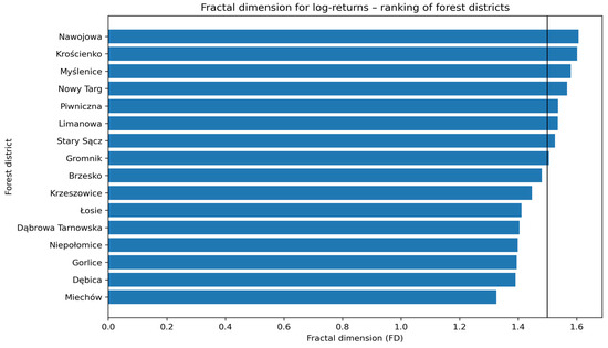
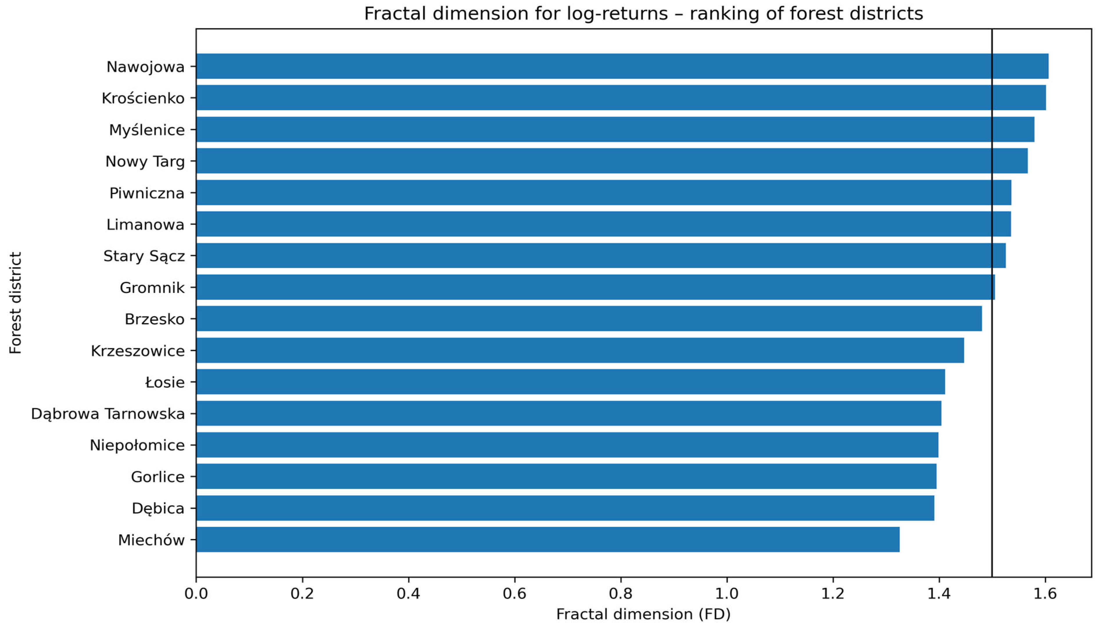
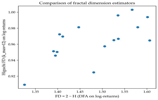
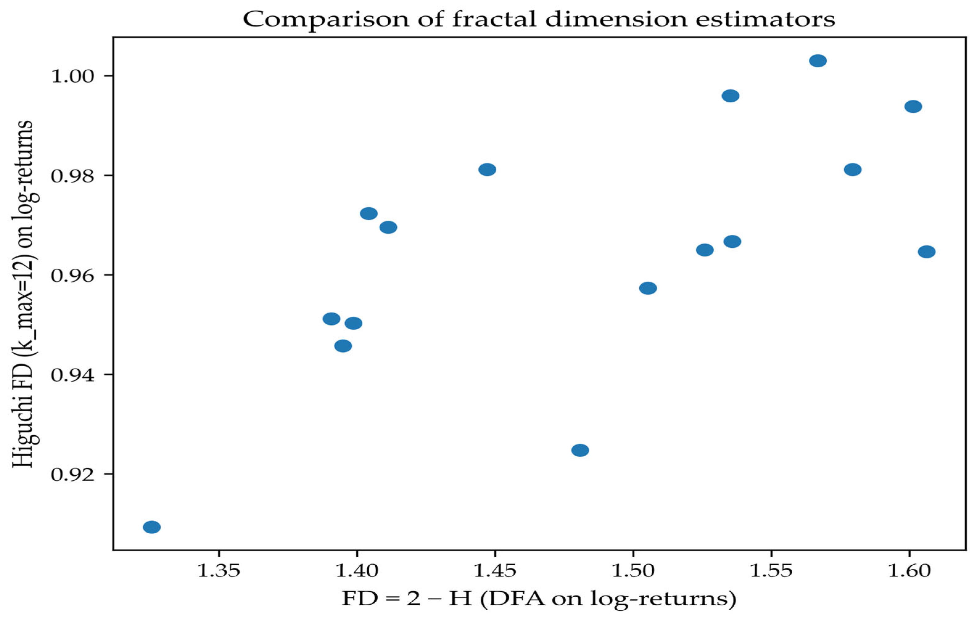
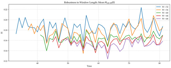
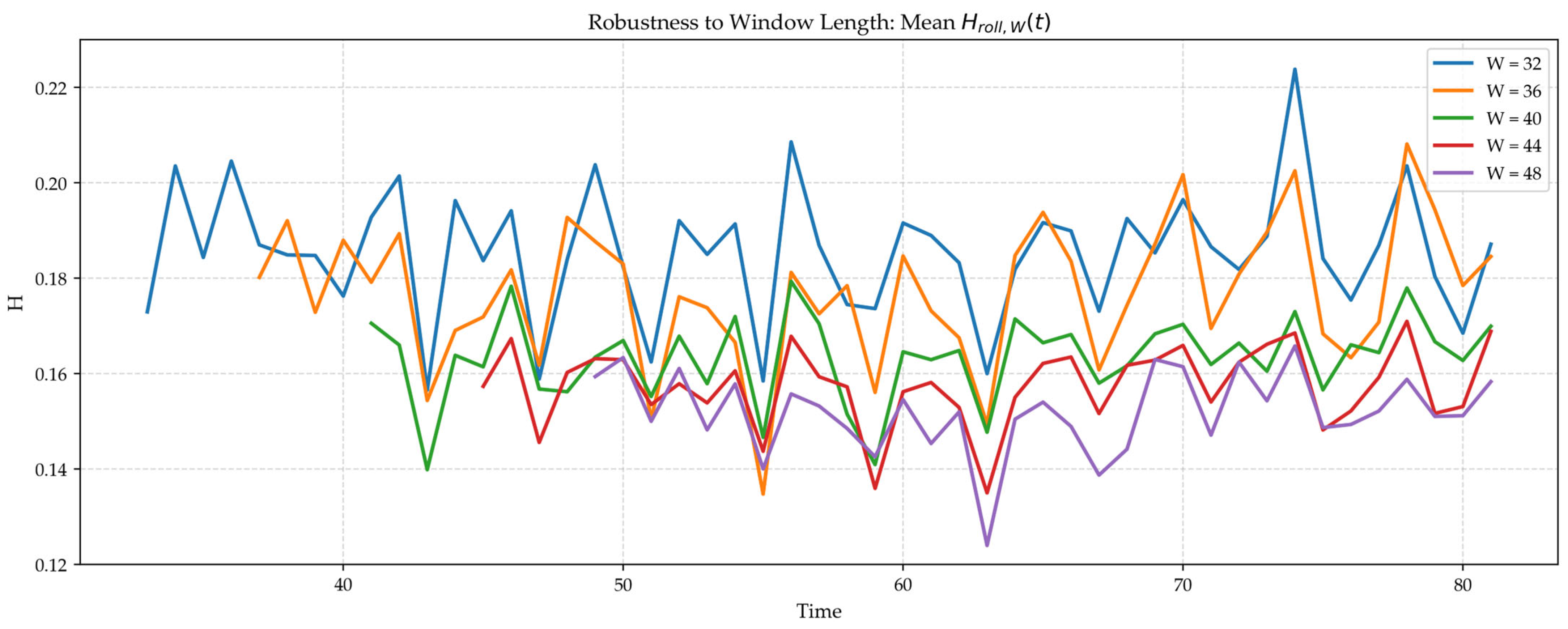
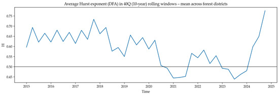
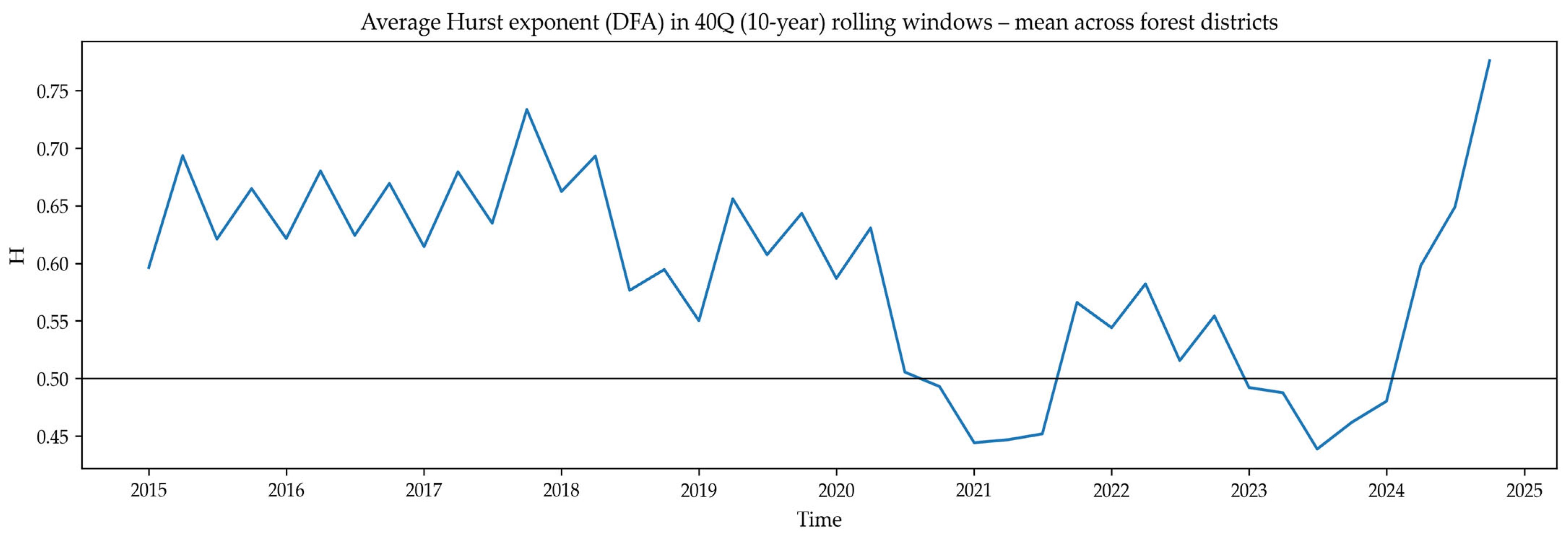
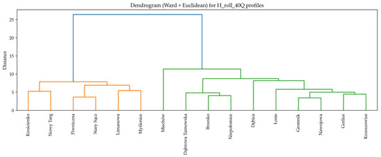
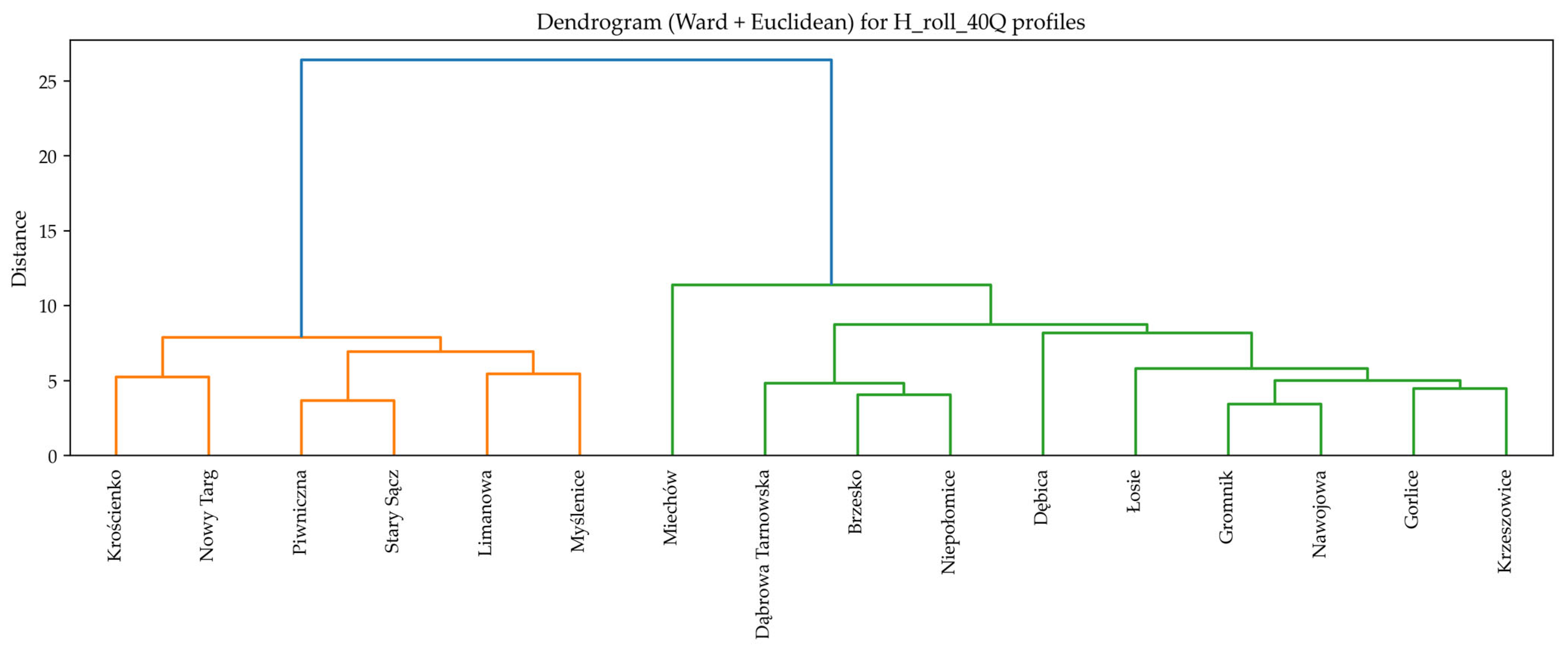
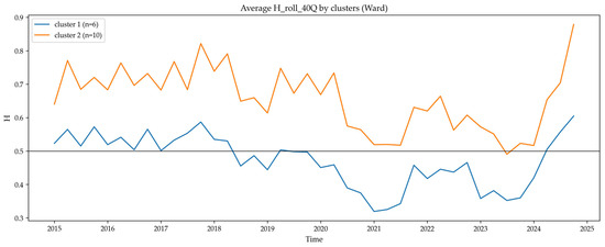
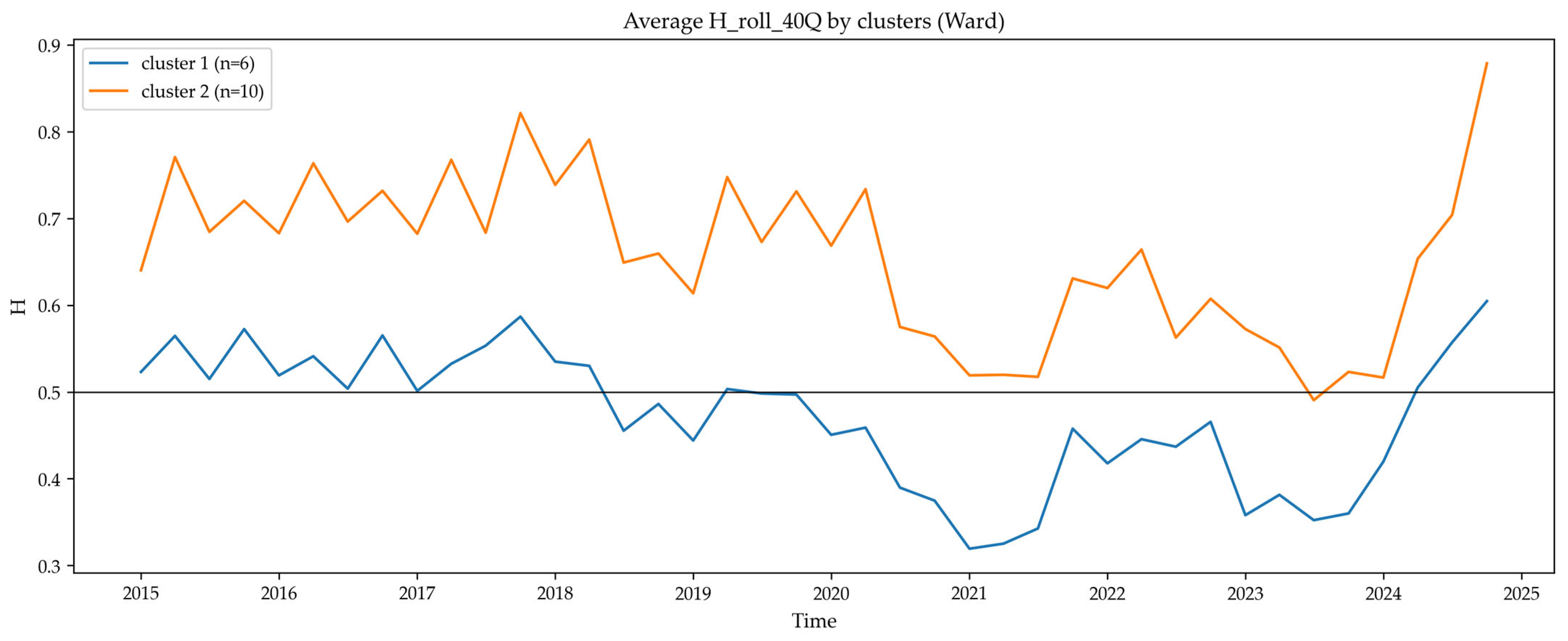
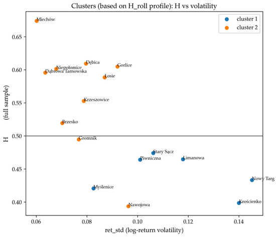
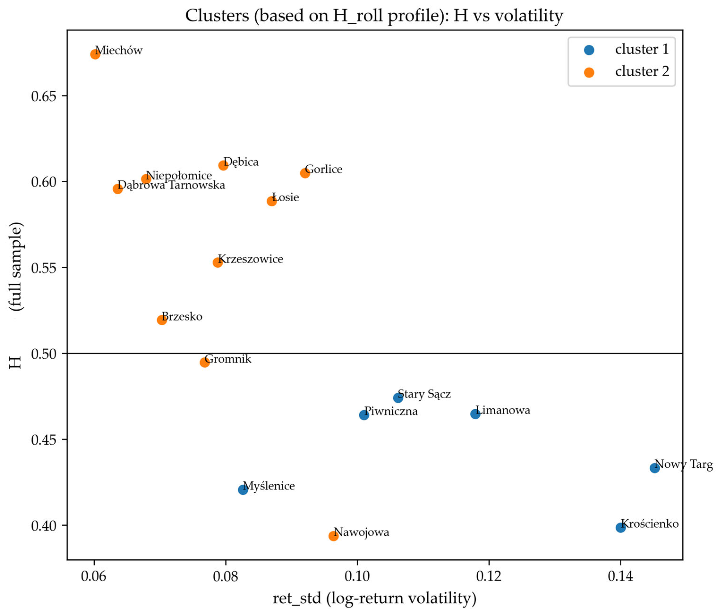
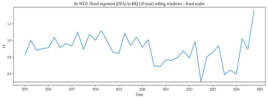
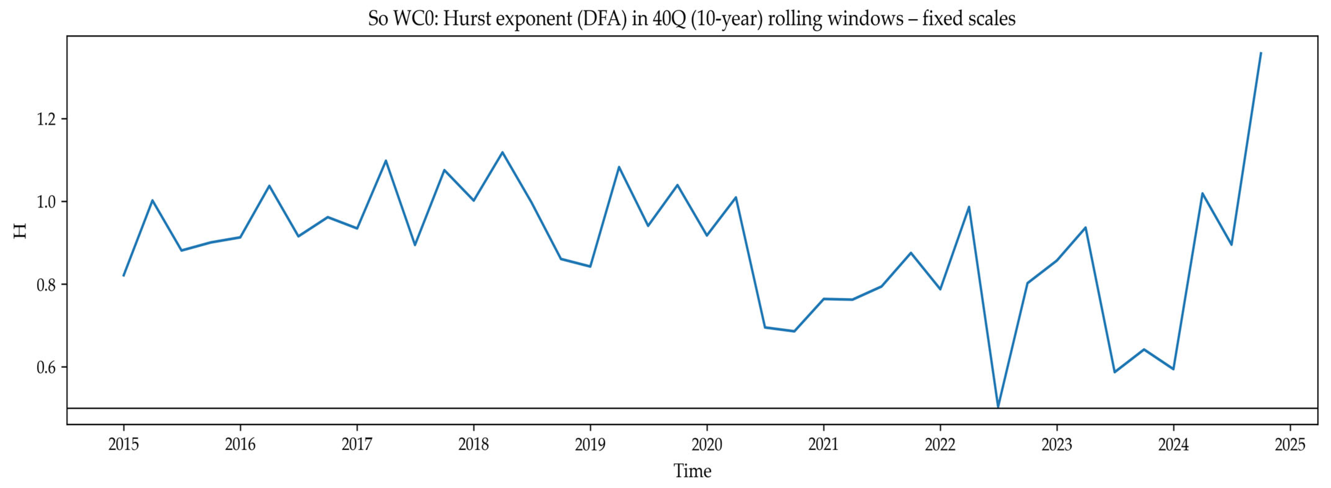

Disclaimer/Publisher’s Note: The statements, opinions and data contained in all publications are solely those of the individual author(s) and contributor(s) and not of MDPI and/or the editor(s). MDPI and/or the editor(s) disclaim responsibility for any injury to people or property resulting from any ideas, methods, instructions or products referred to in the content. |
© 2026 by the authors. Licensee MDPI, Basel, Switzerland. This article is an open access article distributed under the terms and conditions of the Creative Commons Attribution (CC BY) license.