


Abstract
Forest canopy height (FCH) is a fundamental parameter for carbon assessment and ecological monitoring. The Global Ecosystem Dynamics Investigation (GEDI) mission provides full-waveform LiDAR for FCH estimation, yet discontinuous sampling and heterogeneous forests increase uncertainty. Conventional ensemble models rarely account for forest-type-specific structures and remote sensing responses, reducing accuracy and stability. We propose a regional framework combining MBF-Contrast feature selection and a bi-directional stacked model with multi-forest-type feature fusion (BS-MFTF). MBF-Contrast integrates model-based importance with feature-distribution diagnostics to remove redundant and multicollinear variables. BS-MFTF leverages complementarity and structural differences among forest types to improve modeling in heterogeneous canopies. MBF-Contrast reduces feature dimensionality by ~35% versus Mutual Information, Boruta, and RFECV, and improves performance across forest types. BS-MFTF overall achieves R2 = 0.68 (RMSE = 3.22 m; MAE = 2.34 m). Airborne LiDAR validation shows high consistency (R2 = 0.59; RMSE = 1.31 m; MAE = 1.00 m) and a 15%–25% R2 gain over conventional ensembles. The framework offers a scalable solution for large-scale FCH estimation in structurally diverse forests.
1. Introduction
Forests play a crucial role in global carbon cycling, climate regulation, and biodiversity. Forest canopy height (FCH), as a key vertical structural metric, reflects forest structure and supports ecosystem modeling [1,2,3]. The Global Ecosystem Dynamics Investigation (GEDI) mission, a spaceborne full-waveform LiDAR system, provides high-resolution forest canopy height measurements. However, its sparse and discontinuous sampling (approximately 600 m between tracks and 60 m between footprints) limits spatially continuous mapping applications [1,4,5]. To address this limitation, GEDI has been integrated with multi-source remote sensing datasets—including TanDEM-X, Sentinel-1/2, Landsat, and DEMs—alongside advanced feature selection methods such as Recursive Feature Elimination with Cross-Validation (RFECV) and Variance Inflation Factor (VIF) analysis. These integrations have significantly enhanced canopy height estimation accuracy and spatial resolution [6,7,8,9]. Recent studies further demonstrate that combining GEDI and ICESat-2 with Landsat 9 and SRTM data, coupled with random forest-based feature selection, achieves high-accuracy canopy height estimation [10]. Collectively, multi-source fusion exhibits strong potential for generating spatially continuous canopy height products [11]. Despite these advances, estimation accuracy remains heavily dependent on feature selection efficacy. Although diverse algorithms have been deployed, complex canopy structures and stand heterogeneity often induce feature autocorrelation and multicollinearity. Suboptimal feature selection may introduce redundancies, amplify bias, and trigger overfitting, ultimately degrading prediction reliability [12,13,14]. Conventional methods (e.g., RFECV), predominantly those which are model-driven, struggle to capture nonlinear dependencies and exhibit limited noise robustness. Consequently, a hybrid selection framework integrating both model-driven and model-agnostic strategies is essential for robust estimation in complex forest environments.
Beyond feature selection, model architecture profoundly influences canopy height retrieval. Ensemble learning, which combines multiple base learners, has been widely used for forest structural modeling. For instance, an ensemble integrating MLR, SVM, k-NN, and RF with Sentinel-2 and ICESat-2 generated continuous canopy height maps across northern China [15]. Similarly, stacked ensemble models fusing Landsat-8 and PALSAR-2 improved tropical forest height estimation [16], while other studies reduced aboveground biomass (AGB) prediction bias [17]. Overall, ensemble methods enhance model generalization and noise robustness [18,19]. Nevertheless, variability in canopy structure, density, and climate conditions modulates LiDAR and optical responses, increasing modeling complexity. Traditional stacking frameworks, typically comprising base learners and a meta learners, often lack adaptability to diverse forest types [17]. Thus, a novel architecture explicitly incorporating forest-type heterogeneity and enabling cross-layer information exchange is imperative to advance canopy height modeling in structurally complex forests.
This study therefore develops a regional framework for spatially continuous forest canopy height (FCH) mapping by integrating an improved feature selection strategy with a bi-directional stacked model with multi-forest-type feature fusion (BS-MFTF). GEDI waveform-derived metrics are combined with Sentinel-1/2, Landsat-8, and DEM-based variables to construct a multi-source predictor set for regional-scale estimation. To reduce redundancy and improve model robustness in heterogeneous stands, the MBF-Contrast method is implemented by jointly considering model-based importance measures and distributional contrast diagnostics, thereby filtering redundant and multicollinear predictors before model training. Building on the selected feature subsets, BS-MFTF is then constructed to incorporate forest-type heterogeneity through bidirectional stacking, in which forest-type-specific learners are coupled with cross-layer information exchange to exploit complementarity among forest types. In doing so, the proposed framework aims to better capture structural diversity and spatial patterns in complex canopies and to provide a more reliable basis for large-area FCH retrieval and forest structural mapping.
2. Materials and Methods
2.1. Study Area Description
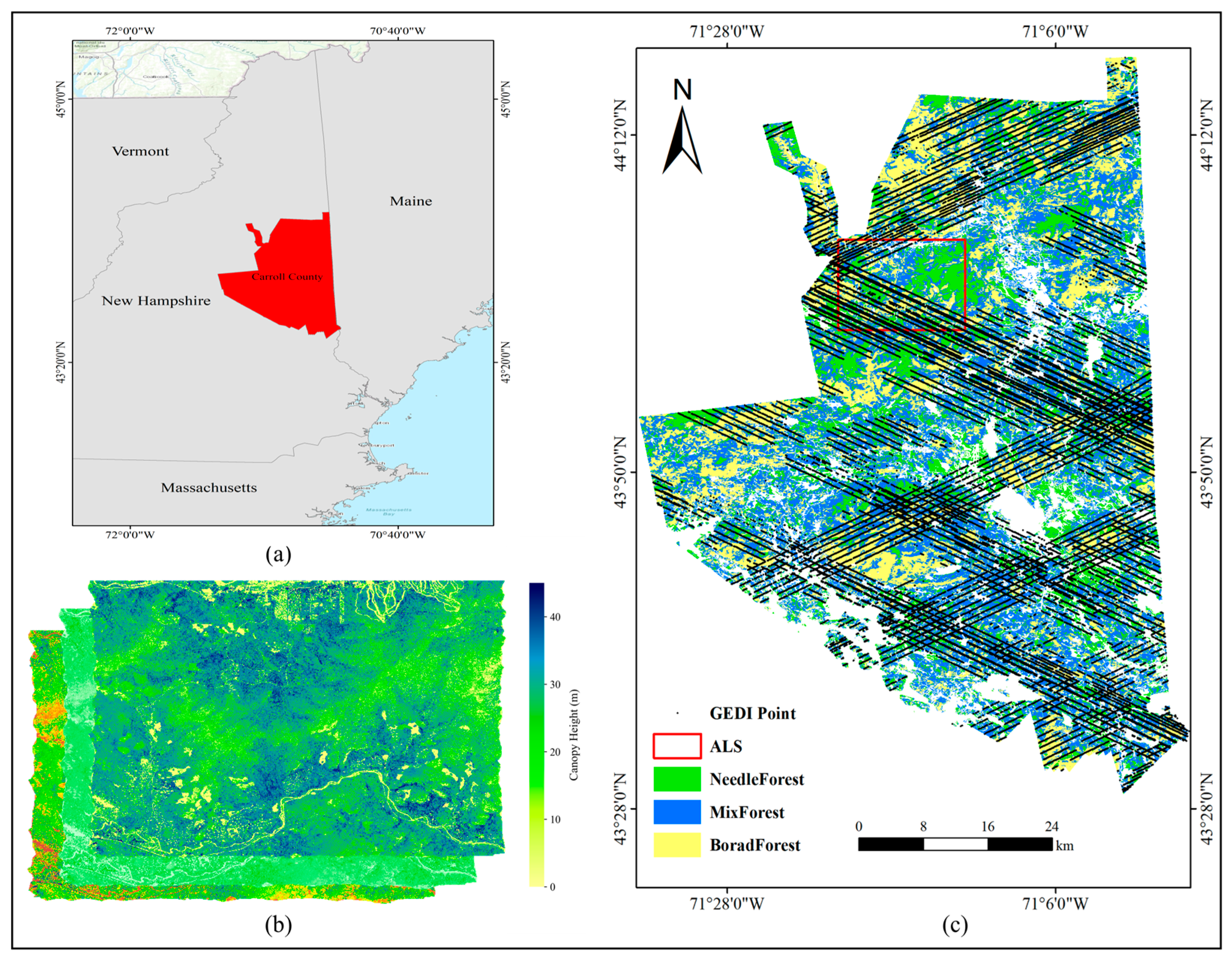
The study area, Carroll County, New Hampshire (~2567 km2), is over 80% forested and characterized by varied terrain. It is centered near 44.0° N, 71.5° W, which helps define the geographic location of the study site. Forests are classified as coniferous (~22%), deciduous (~31%), and coniferous–broadleaf mixed (~47%) based on elevation. Coniferous forests dominate higher areas; deciduous forests occur in lowlands; coniferous–broadleaf mixed forests are found at mid-elevations with diverse canopy structures. This ecological and topographic diversity makes the region ideal for canopy height estimation, multi-type modeling, and forest resource assessment (Figure 1).
Figure 1.
Overview of the study area: (a) Map of the United States showing the location of Carroll County; (b) Airborne LiDAR data coverage; (c) Spatial distribution of forest types and GEDI data footprints within the study area.
2.2. Data
2.2.1. GEDI Data
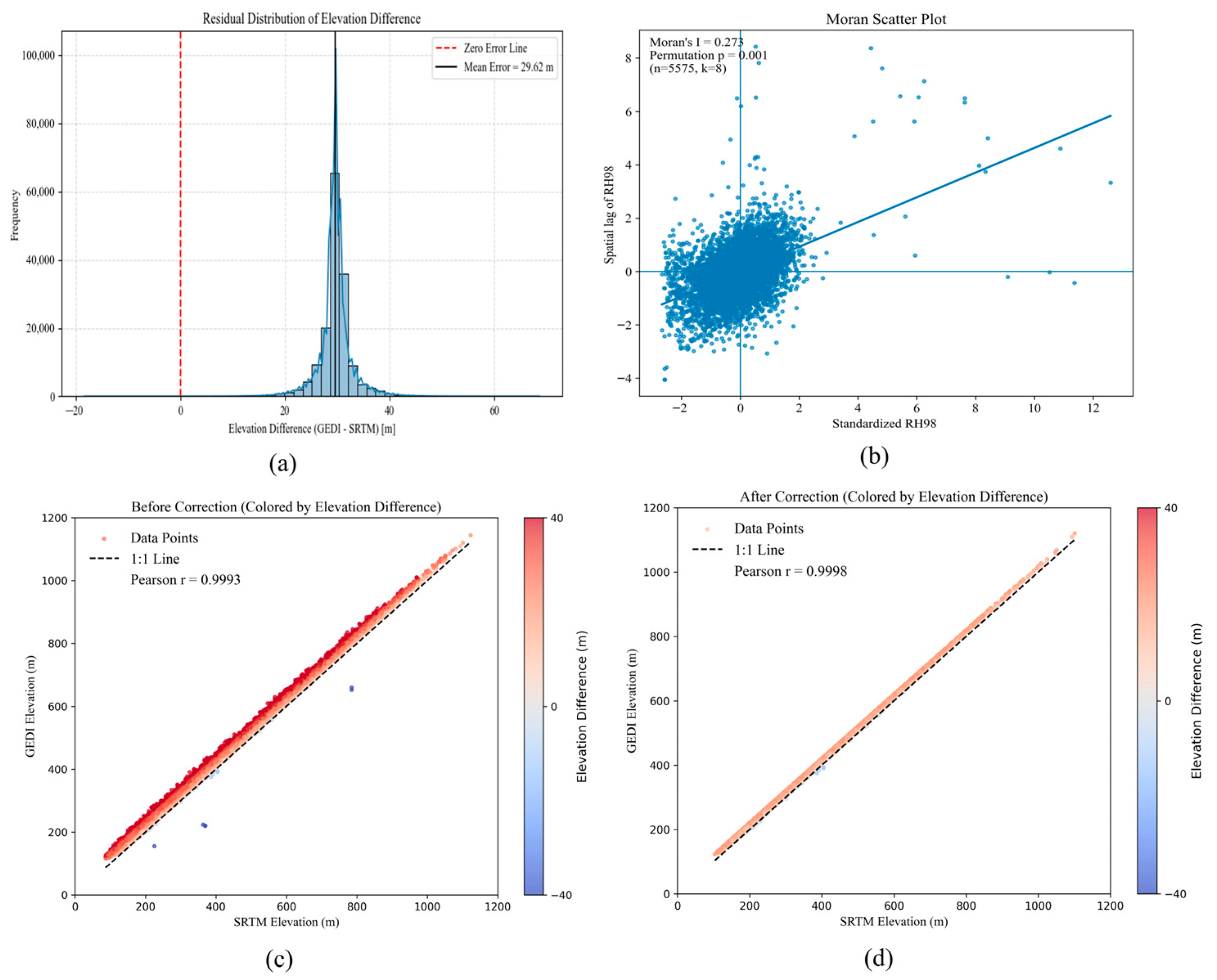
GEDI L2A data (GEDI02_2) were acquired from Google Earth Engine (GEE) for the period March 2021–September 2022. This dataset provides geolocated elevation and canopy height metrics with a ~25 m footprint. To ensure quality, footprints were filtered using quality flags and beam sensitivity (≥0.95) to retain reliable returns. Ground elevation and RH percentiles were extracted [7], and samples with large elevation mismatches with the DEM were removed for topographic correction. In addition, only footprints located on slopes < 30° were retained to avoid waveform distortion in steep terrain. Because RH100 (canopy height percentile based on GEDI Level 2A data, derived from the GEDI LiDAR mission) is highly sensitive to noise and extreme values, RH98 was adopted as a more stable canopy height indicator for modeling [1]. To characterize potential spatial dependence among GEDI footprints, we randomly sampled a subset of footprints () and computed global Moran’s for RH98 using an inverse-distance k-nearest-neighbor (kNN) spatial weights matrix () based on footprint coordinates. The elevation-difference residual distribution, the Moran’s scatter plot for RH98, and the spatial patterns of GEDI footprints before and after terrain correction are summarized in Figure 2.
Figure 2.
GEDI data processing: (a) residual distribution of elevation difference; (b) Moran’s I scatter plot for RH98; (c) GEDI data before terrain correction; (d) GEDI data after terrain correction.
2.2.2. Spatial Distribution Data of Forest Types
The U.S. Geological Survey (USGS) released the first 30 m resolution land cover dataset in 1992, with subsequent updates to the National Land Cover Database (NLCD) enabling systematic monitoring of land cover changes across the contiguous United States [20,21,22]. For this study, forest type data were extracted from the NLCD 2021 Edition [23], covering Carroll County, New Hampshire. Based on the original land cover classification scheme, three forest types were selected: coniferous, deciduous, and coniferous–broadleaf mixed forest. These classes were refined to generate a forest-type distribution map (Figure 1).
2.2.3. Multi-Source Remote Sensing Data
Multiple remote sensing datasets—including Landsat-8, Sentinel-1/2, MODIS, and SRTM DEM (30 m)—were used for spatially continuous canopy height estimation [24,25]. All data were resampled to 30 m for consistency. After preprocessing, spectral reflectance, vegetation indices, texture, polarization, and topographic features were extracted, as shown in Table 1. MODIS was used solely to derive land surface temperature (LST). To reduce scale-mismatch effects, MODIS LST was resampled to 30 m using bilinear interpolation and temporally aggregated (monthly statistics) prior to feature extraction.
Table 1.
Feature parameters extracted from multi-source remote sensing data.
2.2.4. Airborne LiDAR Data
To evaluate FCH inversion accuracy, 1 m-resolution DTM and DSM from airborne LiDAR (NEON, provided by the National Ecological Observatory Network, Boulder, CO, USA) were used to derive CHM by subtracting DTM from DSM [26]. To ensure vertical consistency with GEDI-based products, CHM values referenced to the EGM96 geoid were converted to the WGS84 ellipsoid, removing systematic datum errors. To ensure vertical consistency with GEDI-based products, CHM values referenced to the EGM96 geoid were converted to the WGS84 ellipsoid, removing systematic datum errors. The NEON ALS acquisition was conducted in August 2022, which falls within the GEDI observation period used in this study (March 2021–September 2022), thereby minimizing temporal mismatch between the reference CHM and GEDI-based canopy metrics. To ensure vertical consistency with GEDI-based products, CHM values referenced to the EGM96 geoid were converted to the WGS84 ellipsoid, removing systematic datum errors.
2.3. Methods
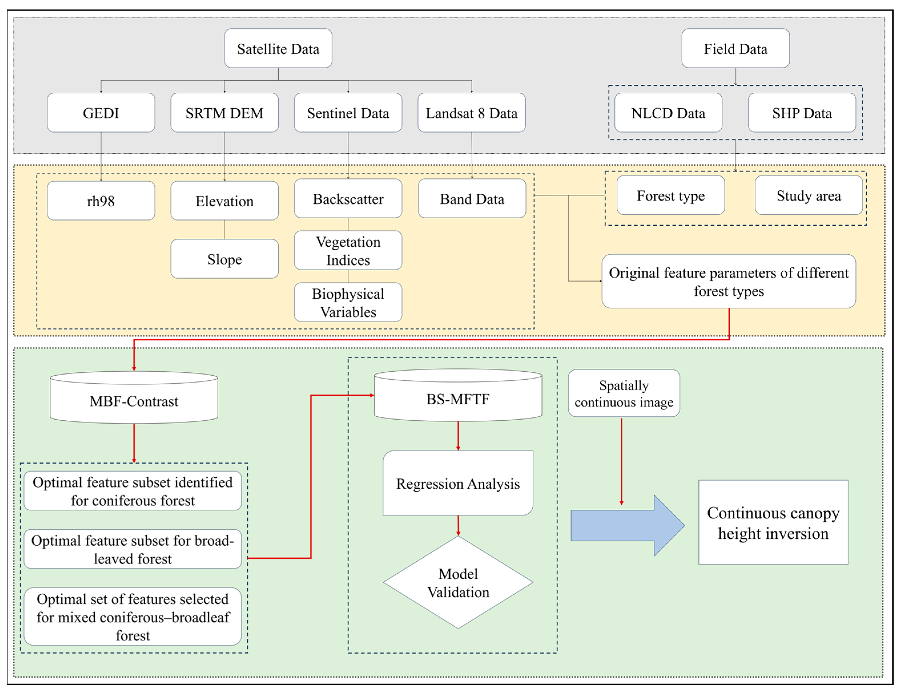
To achieve high-precision and spatially continuous inversion of canopy height in complex heterogeneous forests, this study proposes a novel BS-MFTF framework that integrates GEDI data with multi-source satellite observations. The framework comprises three core components, as illustrated in Figure 3: (1) Based on the spatial distribution data of coniferous, broadleaf, and mixed forests within the study area (Section 2.2), the improved MBF-Contrast feature selection method is independently applied to each forest type to identify optimal feature subsets. (2) Using these optimized feature subsets, the BS-MFTF model was constructed. During the model training phase, the framework exploits structural differences and spatial complementarity among forest types to improve canopy height estimation and regional canopy height mapping. (3) The canopy height products derived from BS-MFTF were rigorously validated using airborne LiDAR data from the NEON program.
2.3.1. MBF-Contrast Feature Selection Method
At local spatial scales, forest canopy height (FCH) varies substantially across forest types because differences in canopy architecture and site conditions modulate LiDAR and optical remote sensing signals. This heterogeneity can induce feature autocorrelation and multicollinearity in multi-source predictors, which may reduce model stability and generalization. Therefore, this study conducts forest-type-specific feature screening for coniferous, broadleaf, and mixed forests to obtain tailored feature subsets for subsequent modeling [24,27].
Figure 3.
Overall technical workflow for canopy height estimation in this study, including multi-source data acquisition, feature extraction and construction, MBF-Contrast feature selection, BS-MFTF modeling, and accuracy validation using NEON/ALS data.
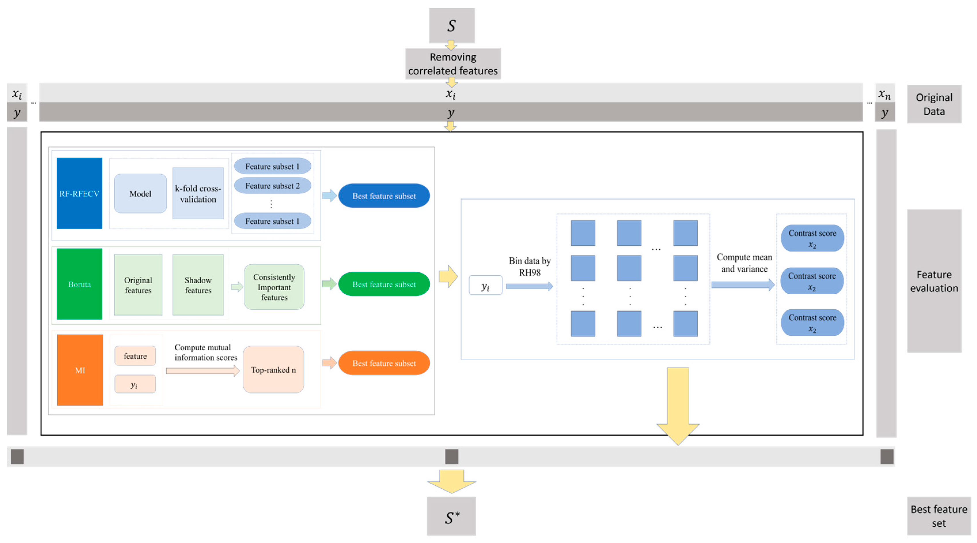
To identify optimal feature subsets for each forest type, we propose MBF-Contrast, an enhanced feature selection framework developed from Random Forest Recursive Feature Elimination (RF-RFE) [28]. RF-RFE recursively removes predictors according to Random Forest-based importance ranking, and the ranking is typically derived from permutation importance and out-of-bag (OOB) error estimation to score each feature and eliminate redundant or irrelevant variables [29]. Rather than directly applying RF-RFE, MBF-Contrast extends it into a multi-stage hybrid screening framework that integrates model-driven importance evaluation with distributional contrast diagnostics (Figure 4).
Figure 4.
MBF-Contrast Framework Process. (In this figure, S represents the original feature set, whereas S* represents the optimal feature subset selected by MBF-Contrast).
Specifically, MBF-Contrast first removes highly correlated predictors using pairwise Pearson correlation coefficients. It then generates candidate feature subsets independently using RFECV, mutual information (MI), and Boruta, and further refines these candidates using a contrast-based method (ContrastFS). Because the original ContrastFS is designed for categorical targets [14], the continuous GEDI RH98 variable is discretized into 20 pseudo-categories to balance stratification granularity and statistical robustness, ensuring sufficient samples within each bin for stable contrast estimation while preserving canopy-height heterogeneity across low, medium, and high ranges. The method then quantifies between-category differences in means and variances to construct a contrast-score matrix, retaining features with higher contrast scores as more discriminative predictors. By combining model-driven and model-free criteria, MBF-Contrast improves robustness and interpretability and yields more reliable feature subsets for canopy height modeling across diverse forest types (Figure 4), The specific steps are as follows:
- (1)
- For each forest type, the training dataset is organized as a feature matrix and a continuous target variable RH98. To reduce redundancy and multicollinearity, pairwise Pearson correlation coefficients are computed among all predictors, and only one variable is retained from each group of strongly correlated features (e.g., ). This yields a decorrelated candidate set for subsequent selection.
- (2)
- Based on the decorrelated candidate feature set, RFECV, Boruta, and mutual information (MI) are applied independently to screen features and identify important variables associated with RH98 from complementary perspectives. The union of the features retained by these three methods forms the initial informative feature pool , which is used for subsequent refinement.
- (3)
- To further refine in a model-agnostic manner, an improved ContrastFS procedure is applied to the continuous target. RH98 is first partitioned into ordered bins (e.g., based on quantiles), representing different canopy height intervals. For each candidate feature and for each pair of bins , the differences in its empirical distributions are summarized using bin-wise means and variances. A global contrast score for feature is then defined as
2.3.2. Bi-Directional Stacking Framework with Multi-Forest-Type Feature Fusion
Forest-type heterogeneity leads to distinct remote sensing responses and model-fitting behaviors across coniferous, broadleaf, and mixed forests. A single global model may therefore yield unstable performance across space, motivating a forest-type-aware integration strategy for spatially continuous FCH inversion [30,31,32].
The proposed BS-MFTF framework constructs type-specific models for the three dominant forest types in the study area. For each forest type, the input predictors are the corresponding compact feature subset selected by MBF-Contrast (Section 2.3.1). Three base learners—Random Forest (RF), XGBoost (XGB), and LightGBM (LGB)—were trained within each forest type, resulting in nine base models in total. To ensure reproducibility and a fair comparison across forest types, the hyperparameters of each base learner were tuned independently within each forest type via grid search, while adopting an identical tuning protocol across types (i.e., the same predefined search spaces, cross-validation scheme, and scoring metric). The optimal hyperparameter set was then selected separately for each forest type. Subsequently, five-fold cross-validation was used to generate out-of-fold predictions, which mitigates overfitting and provides robust level-1 features for subsequent stacking.
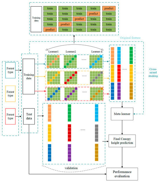
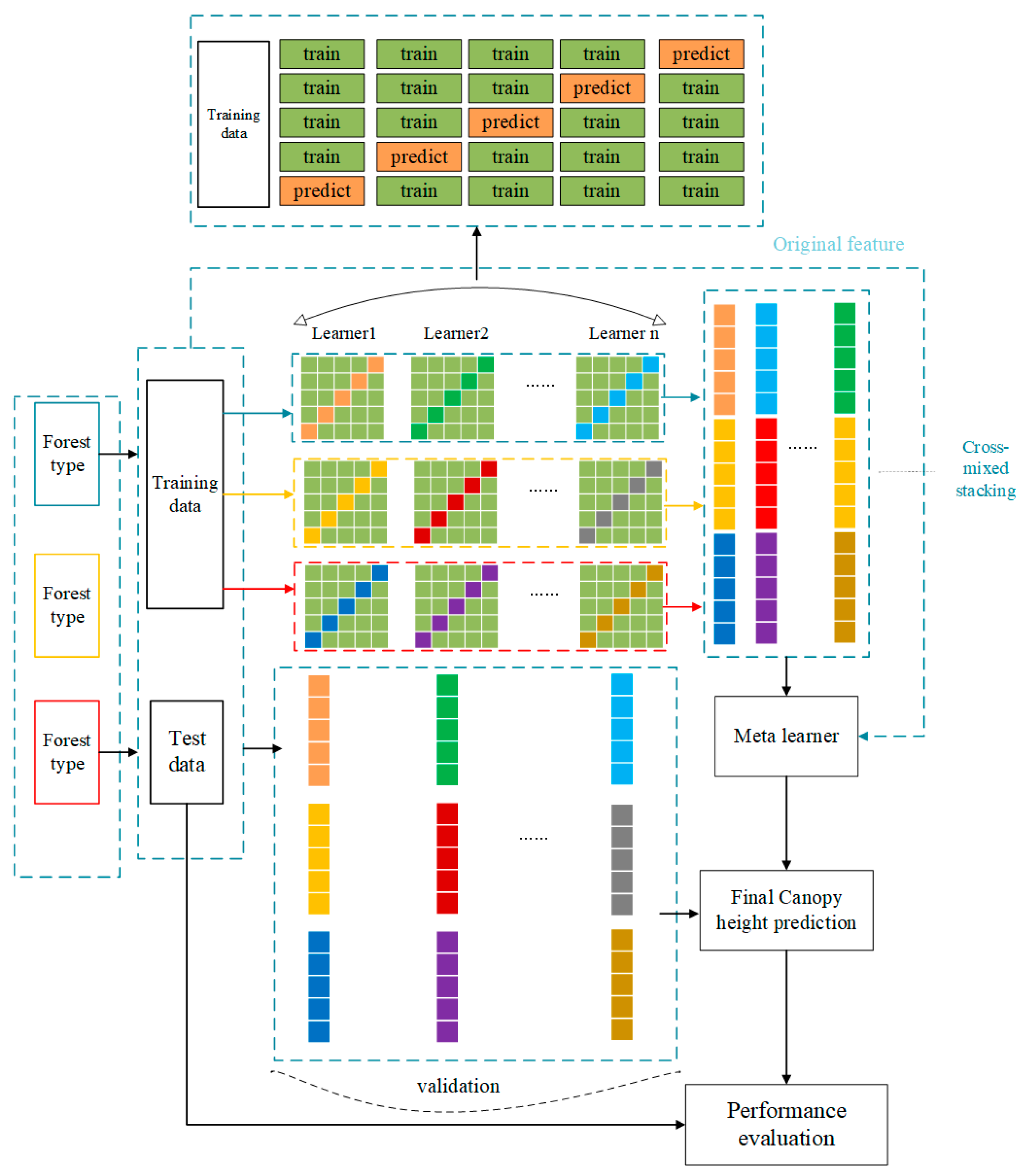
To avoid information fragmentation caused by fully independent type-specific modeling, BS-MFTF adopts a bidirectional stacking scheme with multi-forest-type feature fusion. Specifically, out-of-fold (OOF) predictions from all base models are cross-stacked to form a regional hybrid prediction matrix that aggregates the outputs of each learner–type combination. These OOF-based prediction features are then concatenated to construct the level-1 feature matrix and fed into a ridge regression meta-learner, which enables information exchange and complementarity across forest types and improves regional FCH mapping. For reproducibility, the ridge meta-learner was tuned using the same grid-search protocol (i.e., predefined search space and scoring criterion) as the base learners, and the optimal regularization parameter was selected via five-fold cross-validation on the training set. Importantly, the meta-learner was trained strictly on OOF-derived features to avoid information leakage. The overall workflow is shown in Figure 5, and the specific steps are described as follows:
Figure 5.
Schematic of the BS-MFTF framework. Colored arrows indicate data flows corresponding to different forest types.
- (1)
- For each forest type (coniferous, broadleaf, and mixed forest), the training data are denoted as , where is the feature vector and is the corresponding FCH value. After quality filtering, the sample sizes were 8544 for coniferous forests, 9892 for broadleaf forests, and 7144 for coniferous–broadleaf mixed forests. For each forest type, three model groups are constructed, and each group contains three heterogeneous base learners: Random Forest (RF), XGBoost (XGB), and LightGBM (LGB). The prediction vector of the -th model group for sample in forest type can be written as:
- (2)
- To avoid information leakage and obtain unbiased level-1 inputs, each base learner is trained using K-fold cross-validation. For sample , the OOF (Out-of-Fold) prediction from the -th base learner in group g for forest type is obtained from the model trained without using the fold containing that sample. Specifically, during cross-validation, each fold uses a different subset of the training data, and the samples in that fold are excluded from the training process. The resulting predictions are the OOF predictions. This ensures that each sample does not influence the model training during its prediction, thus avoiding information leakage. The resulting OOF prediction vector is:
- (3)
- To fully exploit model diversity and forest-type information, the OOF prediction matrices from all forest types and model groups are concatenated horizontally to form a regional hybrid prediction matrix:
By fusing prediction features across base learners and forest types, BS-MFTF enables information exchange and complementarity among forest-type-specific models, thereby improving the representation of canopy structure diversity and spatial heterogeneity. This cross-type stacking strategy helps reduce bias and variance relative to single-model baselines and enhances the accuracy and robustness of FCH estimation.
2.4. Traditional Stacking Ensemble for Comparison
For comparison with the proposed BS-MFTF framework, we construct a baseline model using a standard single-layer stacking strategy. The baseline adopts the same base learners (RF, XGBoost, and LightGBM) and the same KKK-fold protocol as BS-MFTF. All samples from different forest types are pooled and treated as a single population, and a unified feature space is used (specifically, the union of the forest-type-specific feature subsets/the original predictor set). The out-of-fold predictions of the base learners are concatenated and fed into one meta-learner, without forest-type-specific training or cross-type stacking. This baseline is referred to as the “traditional ensemble model”:
2.5. Accuracy Assessment
To evaluate the accuracy of the FCH inversion results, we used NEON canopy height model (CHM) data as independent reference data, after unifying them to the WGS84 reference system. All models were trained exclusively with GEDI-derived samples, using RH98 at each footprint as the ground truth FCH; NEON CHM was used only for independent validation and was not involved in model calibration. Within the area of overlap between the NEON site and the predicted FCH map, we constructed a regular grid of circular evaluation plots with a radius of 15 m and a centroid spacing of 30 m. For each plot, the mean predicted FCH and the mean NEON CHM value were extracted through spatial matching and used to fit a regression model for accuracy assessment. The geolocation accuracy of GEDI footprints was also considered in the plot design. Because GEDI shot locations may deviate by several to a few tens of meters, using plot-level mean values rather than single-pixel pairs helps to reduce the influence of small geolocation offsets on the validation statistics. The metrics are defined as follows:
where is the reference value, is the predicted value, and is the number of samples.
3. Results
3.1. Optimal Feature Subset Selection for Different Forest Types Using MBF-Contrast
3.1.1. Correlation Pruning Based on Pearson Correlation
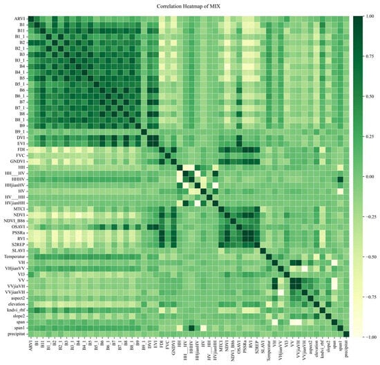
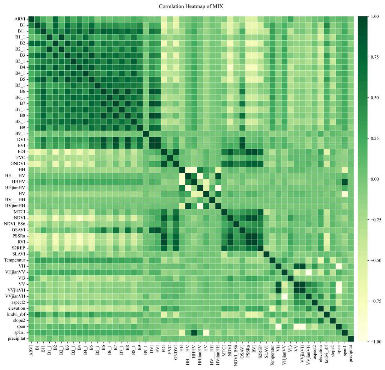
To reduce the impact of multicollinearity among predictors on model training and feature selection, Pearson correlation matrices were computed for the original feature set of each forest type. Since the correlation patterns are broadly consistent across the three forest types, only one representative example is presented to avoid redundancy. Figure 6 shows the correlation structure for the coniferous–broadleaf mixed forest feature set, with numerous strongly correlated feature pairs.
Figure 6.
Pearson correlation heatmap of original features for the coniferous–broadleaf mixed forest in the study area.
As shown in Figure 6, the original feature set contained several highly correlated feature pairs. For each forest type, variables with |r| ≥ 0.9 were excluded. Specifically, in coniferous forests, 18% of the variables were removed; in broadleaf forests, 17% were removed; and in coniferous–broadleaf mixed forests, 22% were removed. This reduction in multicollinearity provides a more stable foundation for subsequent feature selection.
3.1.2. Performance Comparison of Feature Selection Methods
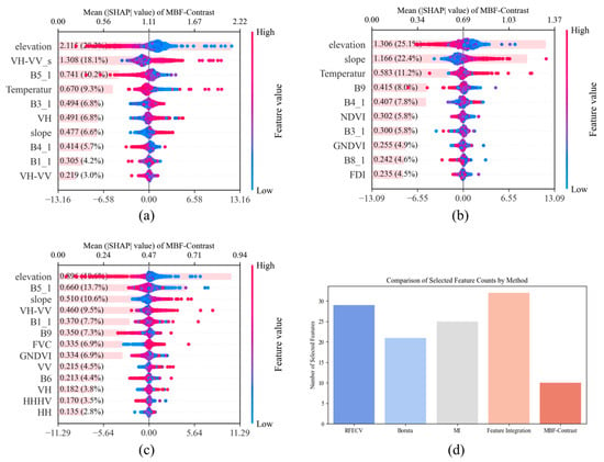
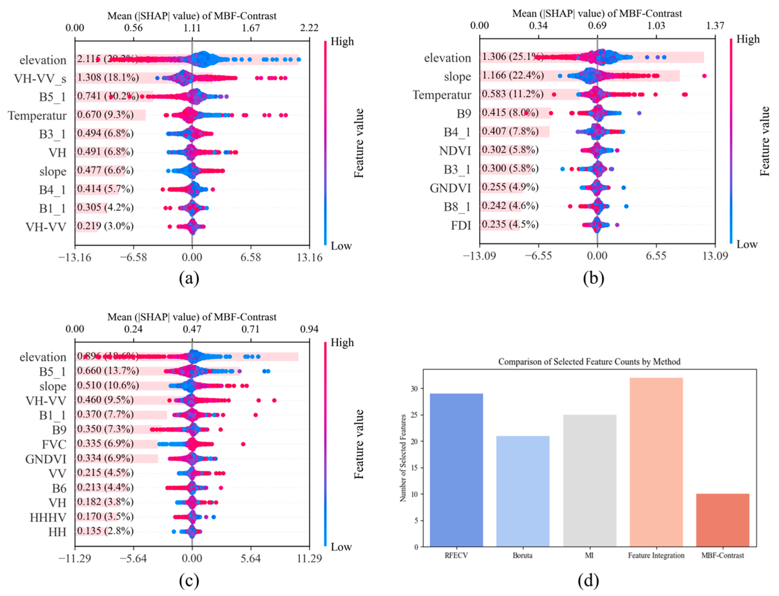
After eliminating highly correlated features, the MBF-Contrast method was employed to further optimize the feature subsets for the three forest types (coniferous forests, broadleaf forests, and mixed forests). This method was systematically compared with commonly used techniques such as RFECV, Boruta, and MI to evaluate its performance. The comparative results are presented in Figure 7:
Figure 7.
SHAP-based interpretation of the MBF-Contrast feature subsets for (a) coniferous forest; (b) broadleaf forest; (c) coniferous–broadleaf mixed forest; (d) comparison of the number of selected features among different feature selection methods for the coniferous forest (shown as a representative example).
The results in Figure 7 indicate that MBF-Contrast effectively reduces feature dimensionality while maintaining, and in some cases improving, model predictive accuracy. Overall, MBF-Contrast shows better feature selection performance and generalization than the competing methods. SHAP-based interpretation further identifies the dominant predictors for each forest type. In coniferous forests, elevation, slope, VH-VV_s (a texture feature derived from the difference between VH and VV polarizations), B5_1, and temperature contribute most to the predictions. Elevation shows a clear negative association with canopy height, suggesting lower canopy height at higher elevations for this forest type. In broadleaf forests, elevation, slope, and temperature are the most influential variables, all positively associated with canopy height. In mixed forests, temperature, B5_1, slope, VH-VV_s, and B1_1 are the primary drivers; elevation again shows a negative association, whereas slope is positively associated with canopy height. Overall, MBF-Contrast identifies interpretable and ecologically meaningful features while removing redundant variables, and its selected predictors remain stable across forest types. These results also highlight forest-type-specific responses to topographic and climatic gradients.
3.2. BS-MFTF Results and Spatial Mapping for Forest Canopy Height
3.2.1. Performance of Forest-Type-Specific Base Learners in the First Layer
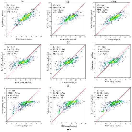
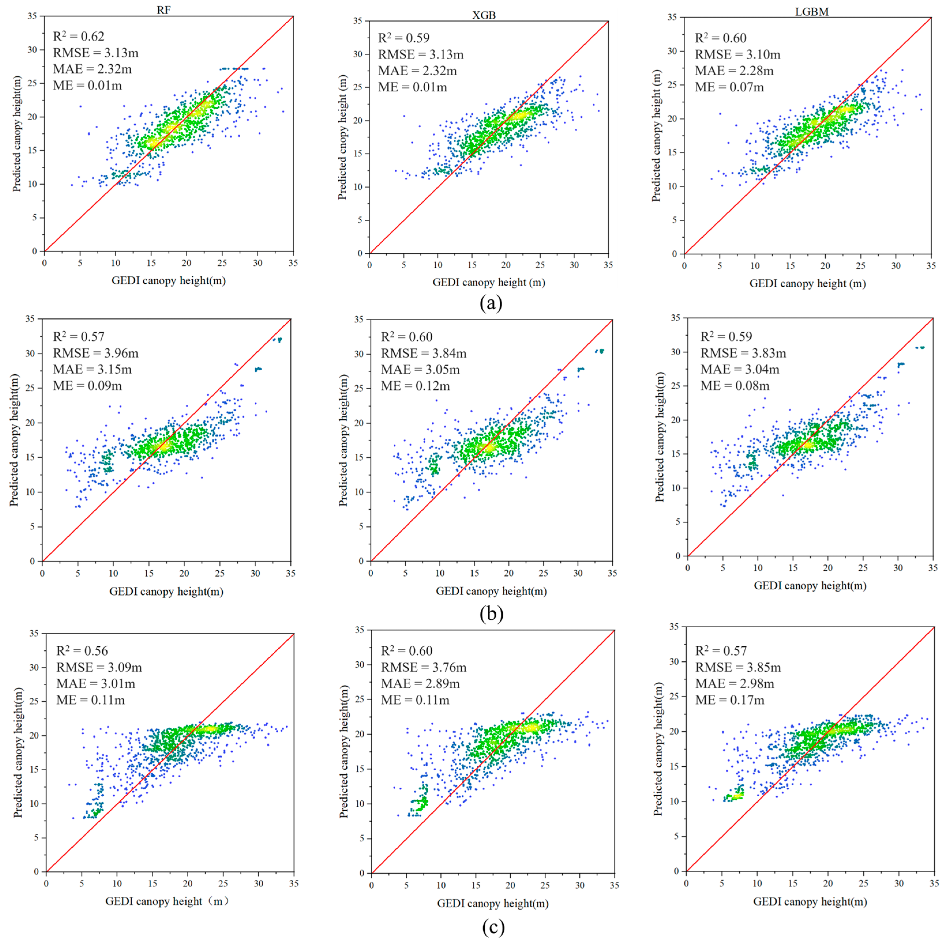
The performance of the nine base regressors (Random Forest, XGBoost, and LightGBM) trained separately for each forest type was evaluated and compared, with the results shown in Figure 8.
Figure 8.
Training results of the base model group: (a) Coniferous forest; (b) Broadleaf forest; (c) Coniferous–Broadleaf mixed forest.
As shown in Figure 8, base-model performance differs across the three forest types (coniferous, broadleaf, and mixed forests), suggesting that forest-type heterogeneity affects model fitting and prediction. In coniferous forests, the best base model achieves = 0.62 with RMSE = 3.00 m, MAE = 2.15 m and ME = 0.01. In broadleaf forests, the optimal base model yields = 0.60, RMSE = 3.84 m, MAE = 3.05 m, and ME = 0.12 m, whereas in mixed forests it attains = 0.60, RMSE = 3.76 m, MAE = 2.89 m, and ME = 0.11 m. Overall, the coniferous-forest models perform consistently better than the other two types across all metrics, indicating that FCH estimation is relatively more reliable for coniferous stands in this study. This advantage may be associated with more homogeneous canopy structure and spatial patterns in coniferous forests, which can produce more stable remote sensing feature responses and stronger predictor–FCH relationships. By contrast, broadleaf and mixed forests exhibit higher RMSE values, implying larger absolute errors and greater sensitivity to local heterogeneity. Possible reasons include more spatially clustered training samples for these two types, which may reduce representativeness across environmental gradients and increase sensitivity to localized outliers. In addition, higher within-type structural variability (e.g., crown density and vertical stratification) may weaken the consistency of feature–FCH relationships and increase uncertainty in height retrieval, thereby constraining overall accuracy.
3.2.2. Base-Model Performance Without Forest-Type Information
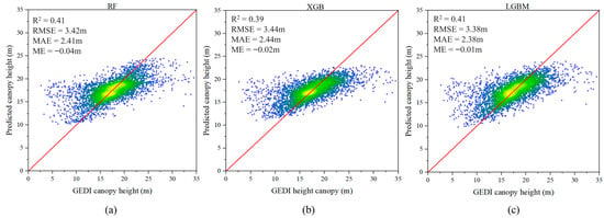
To further validate the importance and feasibility of forest type in canopy height estimation, this study also conducted predictions using the same base model group without incorporating forest type information, as illustrated in Figure 9.
Figure 9.
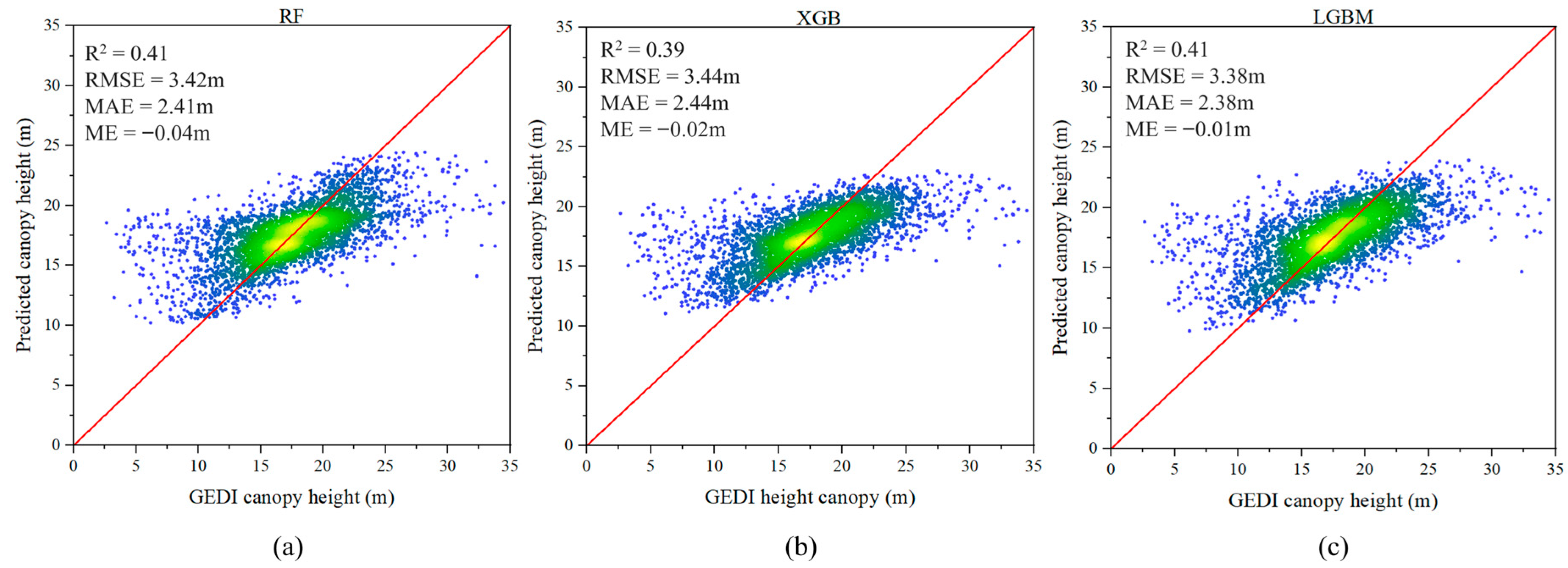
Performance of base learners without forest-type stratification: (a) Random Forest; (b) XGBoost; (c) LightGBM.
Figure 9 summarizes the training and validation performance of the base learners under a pooled setting without forest-type stratification. All three models exhibit modest predictive skill, with values around 0.41 and relatively high RMSE and MAE. The scatter plots further show a clear range-compression effect: predictions concentrate in the mid-range canopy heights, while deviations increase at both low and high height intervals. These results indicate that a forest-type-agnostic pooled strategy cannot adequately represent the structural variability of heterogeneous forests, thereby degrading both accuracy and prediction stability.
3.2.3. Final Predictions and Spatially Continuous FCH Mapping
Based on the outputs in Section 3.2.1 and Section 3.2.2, final predictions were generated using BS-MFTF and a conventional stacking ensemble (without forest-type stratification), and their performance is compared in Figure 10.
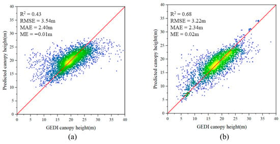
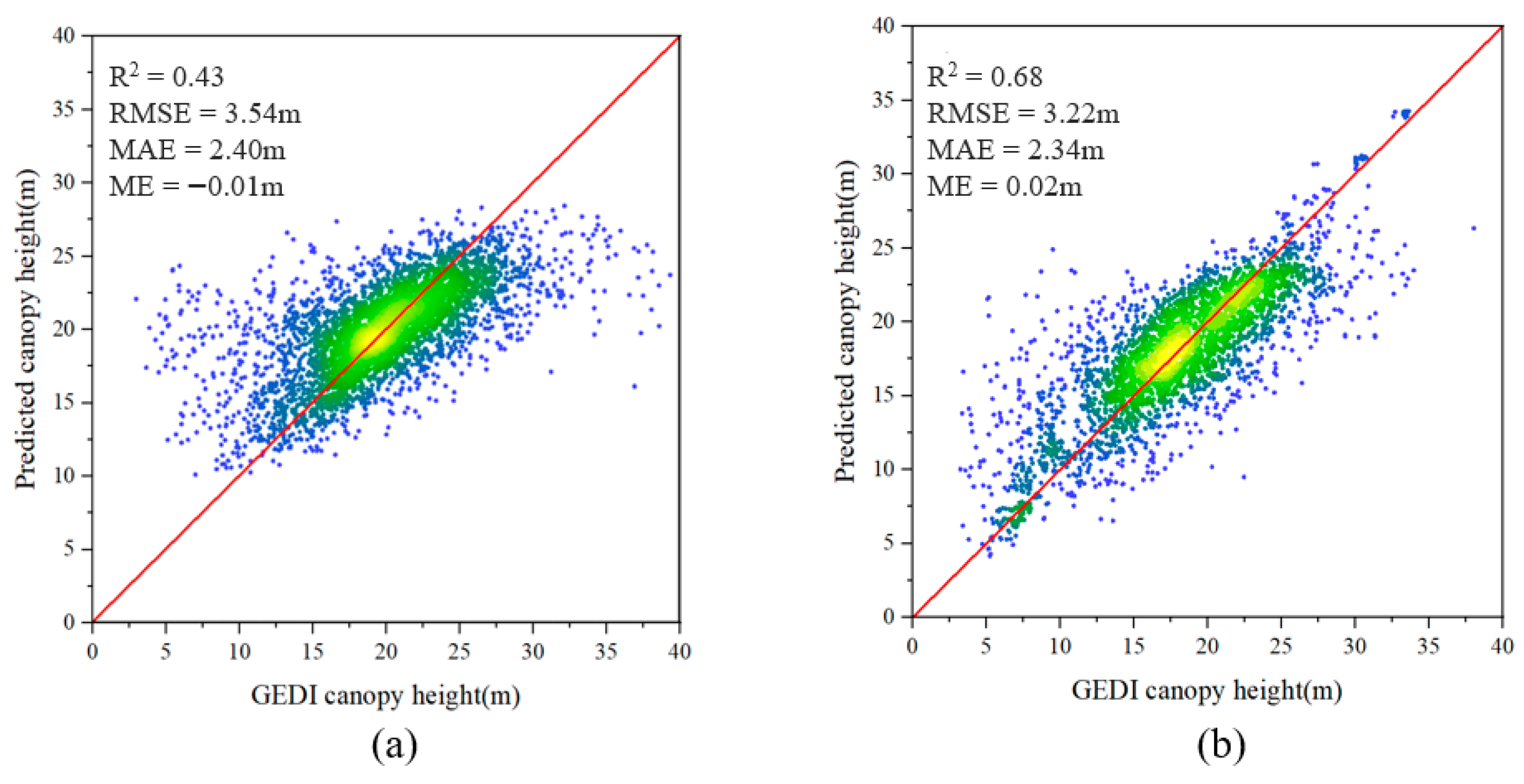
Figure 10.
Final training and validation results of the two models: (a) the traditional ensemble model without forest-type classification and MBF-Contrast-based feature selection; (b) the proposed BS-MFTF model with MBF-Contrast-selected features.
As shown in Figure 10, the traditional ensemble model exhibits a pronounced range-compression effect, with predictions largely concentrated between 5 and 15 m and reduced sensitivity at both low and high canopy-height extremes ( = 0.43). By contrast, the proposed BS-MFTF model maintains consistent performance across the full 0–33 m range, achieving = 0.68, RMSE = 3.22 m, MAE = 2.34 m, and ME = 0.02 m. Compared with the traditional ensemble, BS-MFTF increases by 0.25 (from 0.43 to 0.68; ~58% relative increase) and reduces prediction errors, indicating improved overall estimation performance.
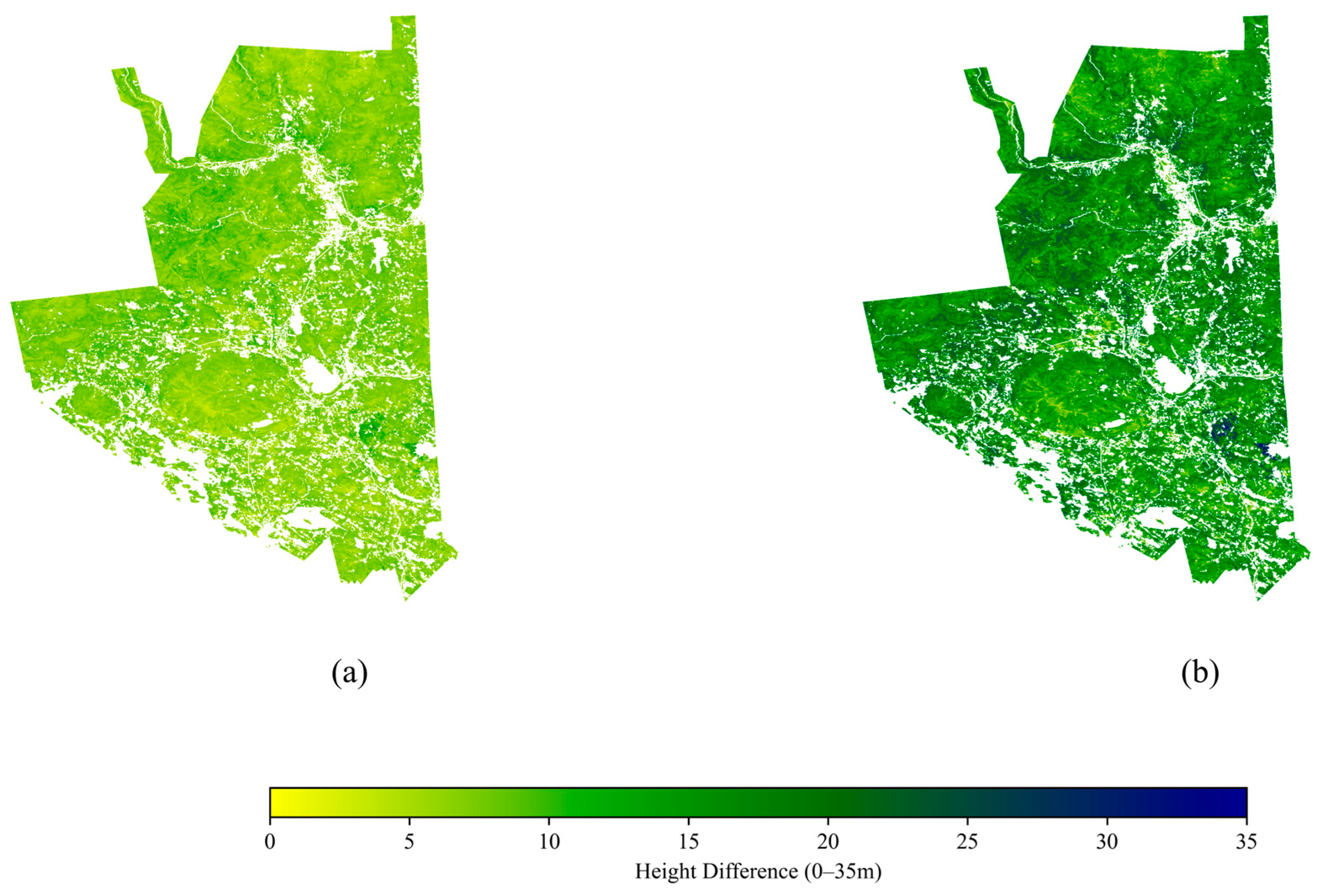
Using the trained traditional ensemble model and BS-MFTF, we generated spatially continuous canopy height predictions for the entire study area; the resulting FCH maps are shown in Figure 11.
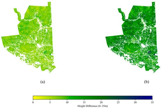
Figure 11.
Continuous forest canopy height maps: (a) traditional ensemble model; (b) BS-MFTF model using features selected by MBF-Contrast.
As shown in Figure 11, the traditional ensemble model shows limited ability to capture extreme canopy heights, with a maximum predicted value of only ~22 m, indicating a clear saturation (range-compression) effect. In contrast, the proposed BS-MFTF model produces a spatially continuous canopy-height pattern across the full 0–33 m range, with peak values reaching ~34 m and improved representation of tall-canopy variability. Overall, these results suggest that BS-MFTF mitigates saturation commonly observed in traditional approaches and enhances the consistency of regional FCH mapping across forest types and canopy-height gradients.
3.3. Airborne LiDAR-Based Validation of FCH Estimates
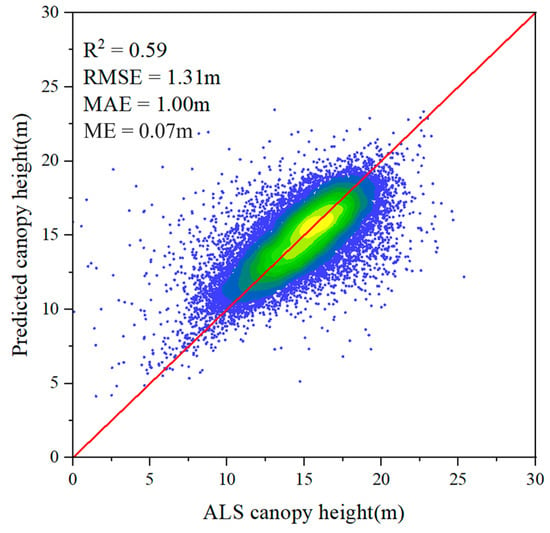
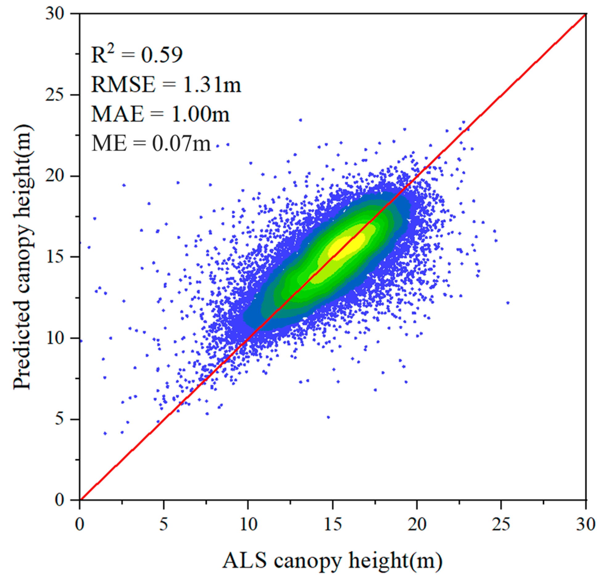
We applied a circular buffer analysis to the airborne LiDAR data and obtained 35,536 validation points to assess the accuracy of the spatially continuous FCH estimates (Figure 12).
Figure 12.
Scatter plot comparing BS-MFTF-predicted canopy height with ALS-derived canopy height for accuracy assessment.
Figure 12 compares BS-MFTF-predicted canopy height with ALS-derived canopy height. Overall, the predictions closely follow the 1:1 line, with most samples concentrated in the mid-height range (approximately 10–20 m) and values spanning ~5–30 m. The validation results show = 0.59, RMSE = 1.31 m, MAE = 1.00 m, and ME = 0.07 m, indicating good agreement between the model estimates and the airborne LiDAR reference. Although scatter increases toward both the lower and higher canopy-height ends, the overall relationship remains stable, suggesting that the proposed framework provides reliable canopy height estimates under heterogeneous conditions in the study area.
3.4. Performance Across RH98-Based Canopy-Height Intervals
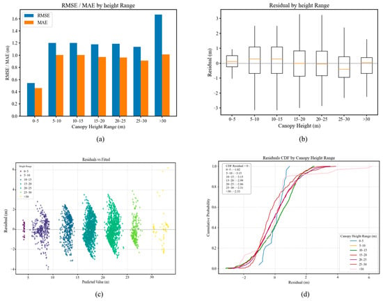
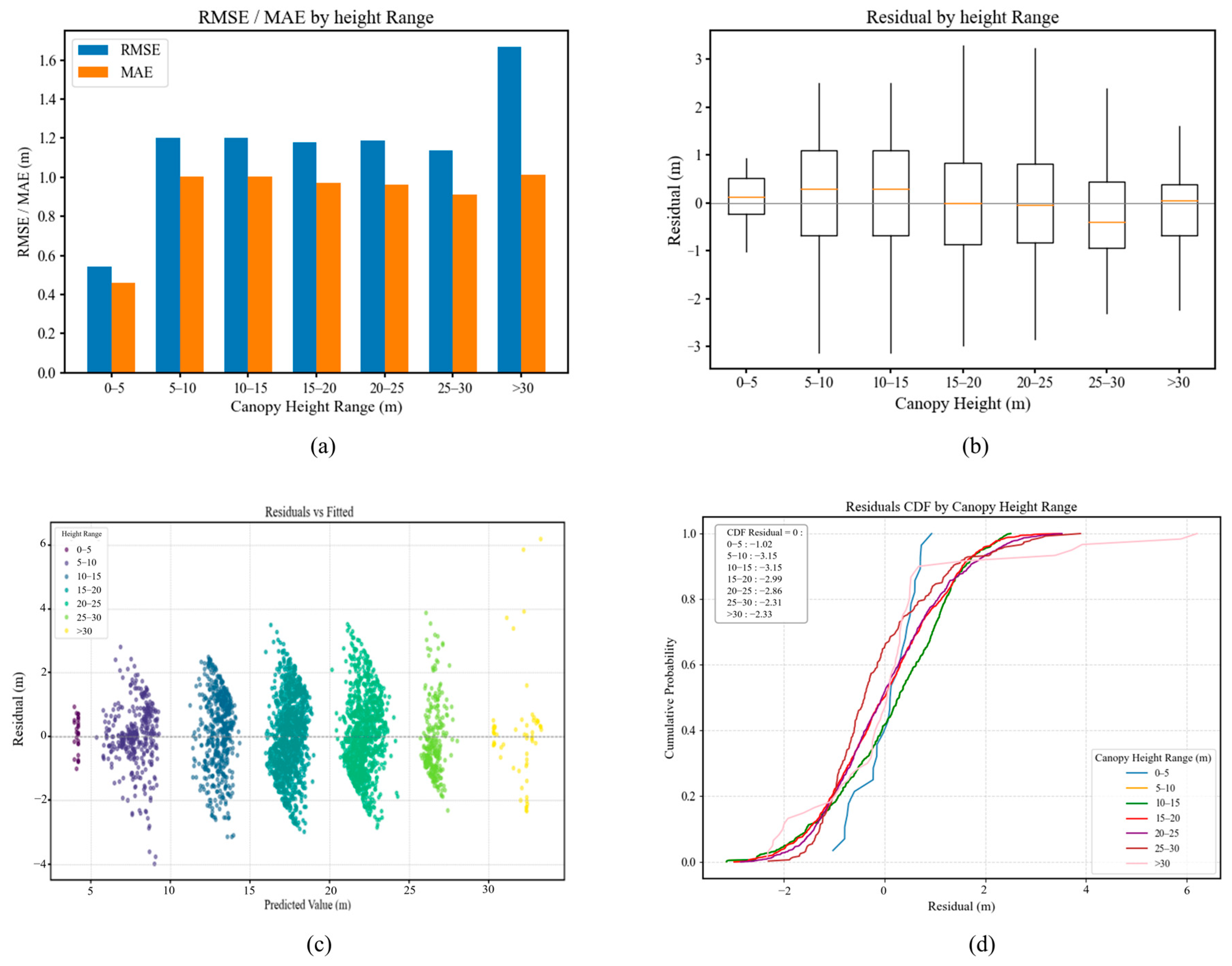
To further examine how model performance varies across canopy-height intervals, we evaluated prediction errors and their cumulative distributions using seven RH98-based height bins (0–5 m, 5–10 m, 10–15 m, 15–20 m, 20–25 m, 25–30 m, and >30 m). The results are shown in Figure 13.
Figure 13.
Performance of the BS-MFTF model across canopy height intervals: (a) RMSE and MAE; (b) residual boxplots; (c) residual scatterplots; (d) cumulative distribution function (CDF) curves.
As indicated by the RMSE and MAE curves in Figure 13, model performance is relatively stable within the 5–30 m canopy-height range but deteriorates markedly above 30 m, where RMSE increases sharply. In the 0–5 m interval, the median residual in the boxplot is positive, and the CDF rises steeply around residual = 0, indicating an overall acceptable bias magnitude but a persistent underestimation (i.e., reference-prediction > 0). This may be related to the strong influence of shrubs, herbaceous vegetation, or bare ground on the remote sensing signal.
In the 5–10 m and 10–15 m intervals, semi-closed vegetation structures and multi-layer foliage can increase the sensitivity of optical and texture features, thereby increasing prediction uncertainty [33]. Residuals remain predominantly positive, and the CDF for the 10–15 m interval becomes less steep and more dispersed, suggesting reduced stability. The 15–20 m interval represents a transition stage, where residuals are more symmetric and the CDF crosses 0.5 at residual = 0, indicating more balanced predictions.
In the 20–25 m interval, the CDF shifts upward, with the cumulative frequency at residual = 0 exceeding 0.5; meanwhile, many points in the residual scatterplot fall below zero, implying a tendency toward overestimation. In the 25–30 m interval, highly closed canopies can cause feature saturation, leading to pronounced underestimation and reduced discrimination [34]. Above 30 m, the residual distribution becomes heavy-tailed, with positive residuals increasing sharply, indicating renewed underestimation that is likely driven by canopy closure and feature saturation.
Overall, model performance varies systematically across canopy-height intervals, showing underestimation at low heights, overestimation at intermediate heights, and renewed underestimation at the upper end.
3.5. Effects of Topographic Factors on FCH Prediction Residuals
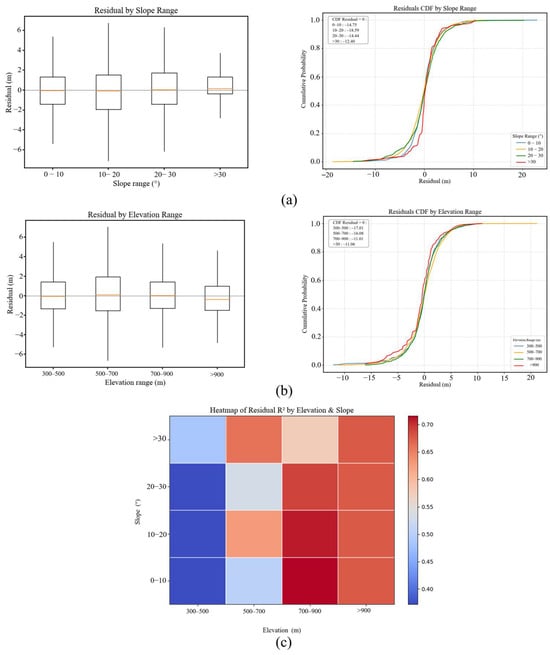
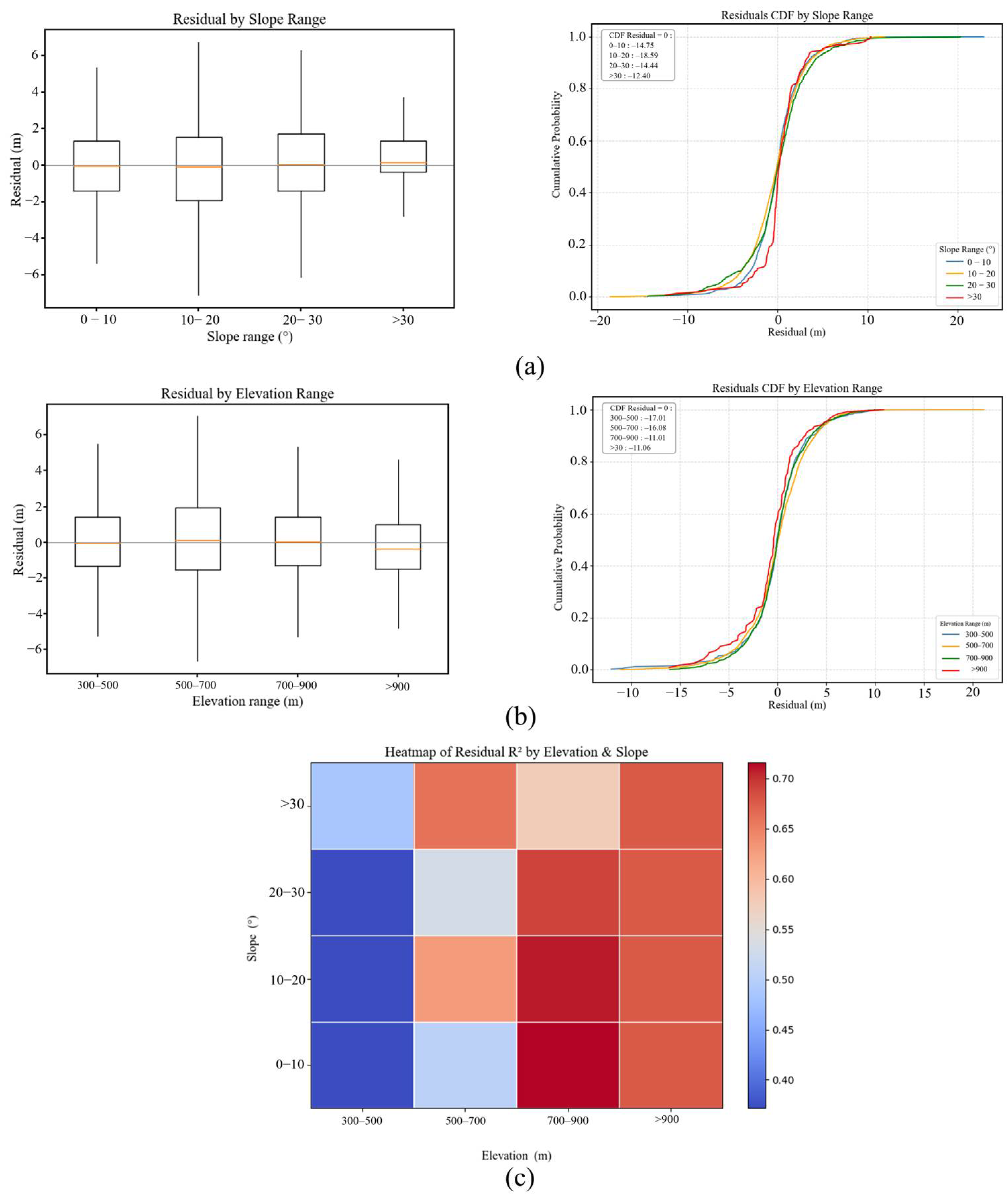
Forest canopy height and structure are strongly influenced by topography, particularly elevation and slope. Therefore, we examined how FCH estimation errors vary with elevation and slope, both individually and in combination, as shown in Figure 14.
Figure 14.
Figure 14 summarizes the error characteristics across topographic strata: (a) residual CDFs for slope intervals; (b) residual CDFs for elevation intervals; (c) a heatmap of for slope–elevation combinations.
As shown in Figure 14a, residuals are more concentrated under gentle slopes, with steeper CDF curves, indicating relatively stable performance. As slope increases, residuals become more dispersed and the CDF curves flatten, suggesting greater error variability and a stronger tendency toward underestimation.
A similar topographic sensitivity is observed along the elevation gradient (Figure 14b). Residual distributions shift systematically with elevation, and the CDF curves show a higher prevalence of positive residuals at higher elevation strata, indicating stronger underestimation in these intervals.
The joint influence of slope and elevation is further illustrated in Figure 14c. Model performance remains weak in low-elevation areas (<700 m), with generally below 0.3 across slope classes. By contrast, performance improves markedly in the mid-to-high elevation range (700–900 m), particularly under gentle slopes where exceeds 0.70. Even under steeper slopes, remains around 0.60, indicating comparatively stable performance under these topographic conditions.
4. Discussion
4.1. Feature Selection and Its Impact on Model Performance
Feature selection is a critical step in high-dimensional modeling because it helps prevent overfitting, reduces computational cost, and can improve predictive performance. Previous studies have investigated multiple feature selection algorithms, including RFECV, Boruta, and MI. RFECV is widely used because it iteratively evaluates model performance via cross-validation [35]. Boruta improves robustness by comparing original predictors with randomized shadow features and has been applied to feature selection in vegetation structure modeling [36]. MI is a model-free scoring approach that is effective for capturing nonlinear relationships between predictors and targets [37]. To enhance FCH prediction through feature selection, we propose a multi-stage framework, MBF-Contrast, which integrates complementary evaluation methods with contrastive analysis of feature distributions. MBF-Contrast first reduces dimensionality using correlation-based filtering and then performs initial screening with RFECV, MI, and Boruta. Continuous variables are subsequently refined using an improved ContrastFS procedure, which combines mean and variance differences across RH98-based height bins to derive the final feature subset. The results show that MBF-Contrast improves prediction accuracy while maintaining a compact predictor set and performs consistently better than individual feature selection methods across forest types.
Unlike approaches that rely solely on model-driven or model-free criteria, MBF-Contrast combines supervised, model-based importance measures with model-agnostic distributional diagnostics. This design helps balance stability and discriminability while accounting for heterogeneity among forest types. Traditional methods often ignore forest-type variability, which can introduce feature-selection bias and lead to unstable model behavior. By adopting bin-wise contrastive evaluation across RH98 canopy-height intervals, MBF-Contrast improves the reliability of selected predictors. The final features are supported by both model importance rankings and clear distributional differences, resulting in more robust feature selection and improved predictive performance.
4.2. Impact of Ensemble Learning on FCH Estimation
With advances in machine learning, ensemble learning has become an important strategy for improving predictive performance. Ensemble algorithms such as Random Forest (RF), XGBoost, and LightGBM have been widely used for estimating canopy height and leaf area index [38,39]. However, many studies do not explicitly incorporate forest-type information and instead treat all samples as a single population, which limits their ability to capture structural differences and complementarity among forest types [40]. In this study, we examine the effects of different ensemble strategies—particularly the proposed BS-MFTF framework and a traditional stacking-based ensemble—on FCH estimation.
To overcome the limitations of conventional ensembles, BS-MFTF builds forest-type-specific base learners for coniferous, broadleaf, and mixed forests in the first layer. Cross-validation is used to generate stable out-of-fold predictions for each forest type, and the second layer performs sample-level cross-stacking of all base-model outputs. This strategy expands the predictive feature matrix while integrating information across forest types. In the meta-model stage, the original predictors (e.g., terrain, spectral, and textural variables) are further included alongside the cross-stacked predictions. By fusing type-specific outputs with raw features, BS-MFTF preserves the strengths of the base learners while improving interpretability and generalization.
Compared with the traditional stacking ensemble, BS-MFTF improves overall accuracy (increasing from 0.43 to 0.68) and enhances performance at both low and high canopy heights, thereby alleviating the prediction range compression observed in conventional ensembles. By jointly leveraging forest-type-specific information and multi-dimensional feature integration, BS-MFTF better represents spatial variability in canopy structure and yields more stable FCH estimates in structurally complex and transitional forest regions.
4.3. Implications of Height-Stratified Performance
The height-interval analysis indicates pronounced height-dependent biases. The model tends to underestimate canopy height in the low-height range (0–5 m), likely influenced by the mixed contributions of low vegetation and ground reflectance. As canopy height increases, errors generally decrease; however, a tendency toward overestimation emerges in the mid-height interval (20–25 m). At the upper end (>25 m), the model again exhibits underestimation, which is consistent with feature saturation under highly closed canopies.
This systematic error pattern highlights the value of height-aware (or height-stratified) modeling strategies for heterogeneous forests. The differing bias directions across low, intermediate, and high canopy-height ranges suggest that the model is sensitive to structural variability that changes with canopy height. Future work could incorporate richer multi-angular or multi-scale texture descriptors and higher-order structural features to improve sensitivity in the low-to-medium height ranges. In addition, integrating complementary canopy height products and developing local bias-correction models for the upper canopy (e.g., >25 m) may further improve performance in challenging tall-canopy regions.
4.4. Topographic Effects and Potential Mitigation
The results above indicate that model errors are topography-dependent and exhibit distinct patterns along both slope and elevation gradients. These patterns likely arise because topography can modulate canopy structure, illumination and shadow conditions, and the quality of remotely sensed signals, thereby altering the stability of feature–target relationships and increasing uncertainty in complex terrain [41].
The slope-related underestimation may reflect greater terrain complexity and spatial heterogeneity of canopy signals on steep slopes, which can weaken the discriminative power of optical and texture predictors and exacerbate saturation effects. Along the elevation gradient, the shift toward more positive residuals at higher elevations indicates stronger underestimation, suggesting that elevation-related differences in canopy conditions and radiometric responses may introduce systematic bias in canopy-top characterization.
To mitigate terrain-related effects, future work could incorporate composite topographic descriptors (e.g., topographic wetness index and terrain complexity index) and adopt more rigorous topographic screening or stratified modeling strategies. In addition, integrating complementary multi-source observations and improving terrain-correction workflows may further enhance the robustness and generalizability of canopy-height estimation in complex terrain.
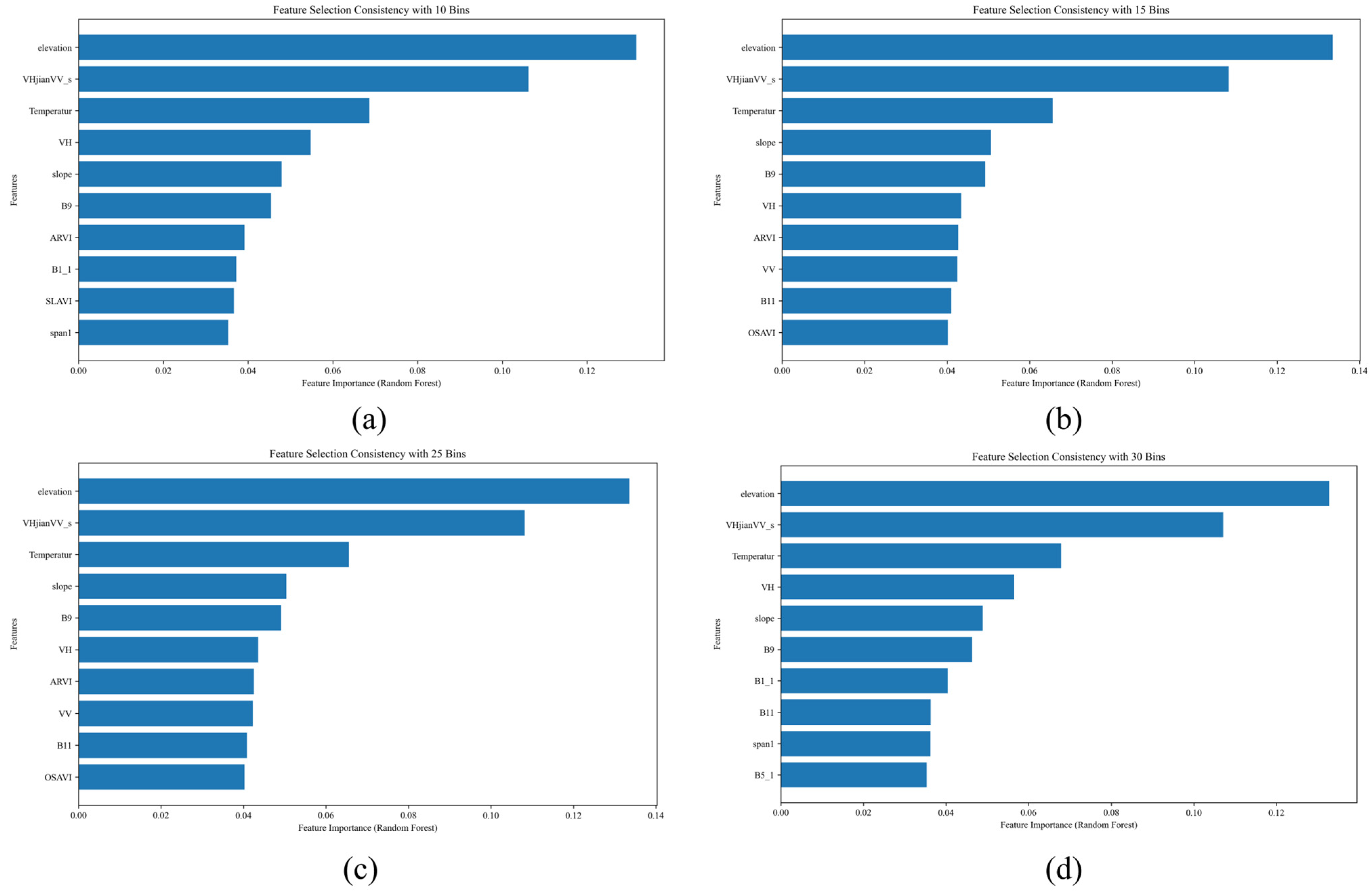
4.5. Effect of Binning Scheme on Feature Selection Stability
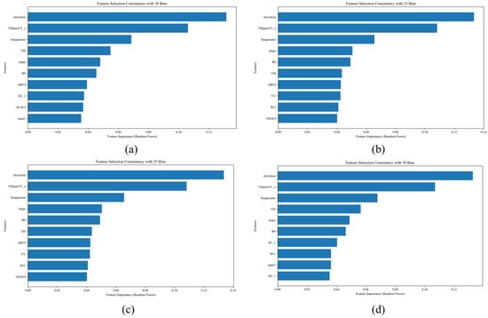
To assess the robustness of MBF-Contrast, we conducted a sensitivity analysis by varying the number of bins used to discretize the GEDI RH98 variable (10, 15, 20, 25, and 30 bins). Using coniferous forests as an example, we applied each binning scheme and evaluated the resulting feature subsets. The selected features remained highly consistent across binning choices, and similar patterns were observed for the other forest types, supporting the robustness and generalizability of MBF-Contrast (Figure 15).
Figure 15.
Features selected by MBF-Contrast under different binning schemes: (a) 10 bins; (b) 15 bins; (c) 25 bins; (d) 30 bins.
Based on these results, we selected 20 bins as a practical compromise between resolution and sample support. Using too few bins (e.g., 10) may smooth out important variability, whereas using too many bins (e.g., 30) can create sparsely populated intervals and yield unstable contrast scores. This choice helps ensure a stable and reliable feature selection process.
4.6. Spatial Autocorrelation and Cross-Validation
In this study, we assessed spatial autocorrelation among GEDI footprints to evaluate its potential influence on cross-validation reliability. Spatial autocorrelation can lead to overly optimistic performance estimates when nearby samples are more similar than expected under random sampling. We quantified spatial autocorrelation using Moran’s I. The results indicated a moderate but statistically significant spatial autocorrelation (Moran’s I = 0.273, p = 0.001).
For model evaluation, we used out-of-fold predictions in cross-validation to avoid direct information leakage from the training set to the validation set. However, we acknowledge that standard (random) cross-validation may not fully eliminate spatial dependence between training and validation folds. Future work could therefore adopt spatially aware evaluation schemes (e.g., spatial blocking or buffered cross-validation) and/or spatial correction methods to further reduce the influence of spatial autocorrelation and provide more robust generalization estimates, especially in areas with strong spatial clustering.
4.7. Explaining Limited RMSE/MAE Improvements and Evaluating Systematic Bias
The relatively limited reductions in RMSE and MAE may partly reflect the distribution of training samples: mid-to-high canopy heights dominate the dataset, whereas very low and very high canopy conditions are under-represented. As a result, model learning is driven mainly by the central height range, which constrains further error reduction in the distribution tails. By contrast, systematic bias remains small across all settings (ME = 0.01–0.17 m), indicating no pronounced overall over- or underestimation. Therefore, the remaining errors are more likely dominated by unsystematic components (e.g., footprint–pixel mismatch, canopy structural heterogeneity, and measurement noise) rather than a consistent offset, although localized tail errors may persist due to sample scarcity.
Future work will focus on improving tail performance through distribution-aware training (e.g., RH98-stratified sampling and re-weighting of under-represented intervals) and more fine-grained diagnostics (interval-specific errors and within-stratum ME tests), with bias correction or calibration applied if localized biases are detected.
5. Conclusions
This study proposes an integrated framework for forest canopy height (FCH) estimation in structurally heterogeneous forests by combining MBF-Contrast feature selection with the BS-MFTF ensemble model, enabling spatially continuous FCH mapping at 25 m resolution. Compared with conventional approaches that pool all samples and train a single global model (or apply standard stacking on pooled data), BS-MFTF differs in three key aspects.
First, BS-MFTF is explicitly forest-type-aware as it trains separate base learners for coniferous, broadleaf, and mixed forests using compact, type-specific feature subsets selected by MBF-Contrast. This design allows the model to accommodate structural and radiometric differences among forest types, rather than forcing one set of predictors and one mapping function to fit all conditions. Second, BS-MFTF performs cross-type fusion at the stacking stage. Instead of stacking only within a pooled sample space, the meta-learner integrates cross-stacked predictions from all forest-type-specific base models, thereby exploiting information complementarity across forest types and reducing the range compression (saturation) behavior observed in conventional ensembles. Third, BS-MFTF augments the meta-model inputs by jointly using cross-stacked predictions and the original remote sensing predictors (terrain, spectral, and textural variables). This multi-source, multi-level fusion enriches the predictive representation and improves the spatial consistency of regional FCH mapping.
Independent validation against airborne LiDAR supports the reliability of the mapped products, indicating that the proposed framework is suitable for regional-scale canopy structure monitoring in heterogeneous landscapes. Future work will focus on (i) improving performance in complex terrain and extreme canopy-height conditions by integrating higher-resolution and multi-temporal observations and strengthened terrain correction, (ii) enhancing sample representativeness for under-represented height ranges through distribution-aware training and targeted sampling, and (iii) extending the framework to additional regions and related structural attributes, such as aboveground biomass.
Author Contributions
Conceptualization, Z.W. and H.Y.; methodology, Z.W., J.D. and H.Y.; formal analysis, J.H. and J.C.; data curation, Y.L.; validation, Y.L. and J.C.; writing—original draft preparation, Z.W. and H.Y.; writing—review and editing, Z.W., J.D. and H.Y.; supervision, J.H. All authors have read and agreed to the published version of the manuscript.
Funding
This study was supported by grants from the National Natural Science Foundation of China (42261063), Guangxi Science and Technology Base and Talent Special Project (Grant No. GuikeAD23026263), BaGui Young Outstanding Talents Cultivation Program of the provincial government of Guangxi, and Scientific Research Foundation of Guilin University of Technology (GLUTQD2017094).
Data Availability Statement
The data presented in this study are available from the corresponding author by reasonable request.
Conflicts of Interest
The authors declare no conflicts of interest.
References
- Qi, W.; Armston, J.; Choi, C.; Stovall, A.; Saarela, S.; Pardini, M.; Fatoyinbo, L.; Papathanassiou, K.; Pascual, A.; Dubayah, R. Mapping large-scale pantropical forest canopy height by integrating GEDI lidar and TanDEM-X InSAR data. Remote Sens. Environ. 2025, 318, 114534. [Google Scholar] [CrossRef] [Scilit]
- Goetz, S.; Dubayah, R. Advances in remote sensing technology and implications for measuring and monitoring forest carbon stocks and change. Carbon Manag. 2011, 2, 231–244. [Google Scholar] [CrossRef] [Scilit]
- Asner, G.P.; Mascaro, J.; Muller-Landau, H.C.; Vieilledent, G.; Vaudry, R.; Rasamoelina, M.; Hall, J.S.; van Breugel, M. A universal airborne LiDAR approach for tropical forest carbon mapping. Oecologia 2012, 168, 1147–1160. [Google Scholar] [CrossRef] [Scilit]
- Potapov, P.; Li, X.; Hernandez-Serna, A.; Tyukavina, A.; Hansen, M.C.; Kommareddy, A.; Pickens, A.; Turubanova, S.; Tang, H.; Silva, C.E.; et al. Mapping global forest canopy height through integration of GEDI and Landsat data. Remote Sens. Environ. 2021, 253, 112165. [Google Scholar] [CrossRef] [Scilit]
- Dubayah, R.; Blair, J.B.; Goetz, S.; Fatoyinbo, L.; Hansen, M.; Healey, S.; Hofton, M.; Hurtt, G.; Kellner, J.; Luthcke, S.; et al. The Global Ecosystem Dynamics Investigation: High-resolution laser ranging of the Earth’s forests and topography. Sci. Remote Sens. 2020, 1, 100002. [Google Scholar] [CrossRef] [Scilit]
- Su, Y.; Ma, Q.; Guo, Q. Fine-resolution forest tree height estimation across the Sierra Nevada through the integration of spaceborne LiDAR, airborne LiDAR, and optical imagery. Int. J. Digit. Earth 2017, 10, 307–323. [Google Scholar] [CrossRef] [Scilit]
- Schlund, M.; Wenzel, A.; Camarretta, N.; Stiegler, C.; Erasmi, S. Vegetation canopy height estimation in dynamic tropical landscapes with TanDEM-X supported by GEDI data. Methods Ecol. Evol. 2023, 14, 1639–1656. [Google Scholar] [CrossRef] [Scilit]
- Wu, Z.; Yao, F.; Zhang, J.; Ma, E.; Yao, L.; Dong, Z. Genetic Programming Guided Mapping of Forest Canopy Height by Combining LiDAR Satellites with Sentinel-1/2, Terrain, and Climate Data. Remote Sens. 2024, 16, 110. [Google Scholar] [CrossRef] [Scilit]
- Liu, A.; Chen, Y.; Cheng, X. Improving Tropical Forest Canopy Height Mapping by Fusion of Sentinel-1/2 and Bias-Corrected ICESat-2–GEDI Data. Remote Sens. 2025, 17, 1968. [Google Scholar] [CrossRef] [Scilit]
- Zhu, W.; Li, Y.; Luan, K.; Qiu, Z.; He, N.; Zhu, X.; Zou, Z. Forest Canopy Height Retrieval and Analysis Using Random Forest Model with Multi-Source Remote Sensing Integration. Sustainability 2024, 16, 1735. [Google Scholar] [CrossRef] [Scilit]
- Lang, N.; Jetz, W.; Schindler, K.; Wegner, J.D. A high-resolution canopy height model of the Earth. Nat. Ecol. Evol. 2023, 7, 1778–1789. [Google Scholar] [CrossRef] [Scilit]
- Meyer, H.; Reudenbach, C.; Wöllauer, S.; Nauss, T. Importance of spatial predictor variable selection in machine learning applications—Moving from data reproduction to spatial prediction. Ecol. Model. 2019, 411, 108815. [Google Scholar] [CrossRef] [Scilit]
- Du, R.; Lu, J.; Xiang, Y.; Zhang, F.; Chen, J.; Tang, Z.; Shi, H.; Wang, X.; Li, W. Estimation of winter canola growth parameter from UAV multi-angular spectral-texture information using stacking-based ensemble learning model. Comput. Electron. Agric. 2024, 222, 109074. [Google Scholar] [CrossRef] [Scilit]
- Cao, C.; Zhang, Q.; Deng, Y. A contrast based feature selection algorithm for high-dimensional datasets in machine learning. Inf. Sci. 2025, 717, 122308. [Google Scholar] [CrossRef] [Scilit]
- Jiang, F.; Zhao, F.; Ma, K.; Li, D.; Sun, H. Mapping the Forest Canopy Height in Northern China by Synergizing ICESat-2 with Sentinel-2 Using a Stacking Algorithm. Remote Sens. 2021, 13, 1535. [Google Scholar] [CrossRef] [Scilit]
- Liu, A.; Chen, Y.; Cheng, X. Evaluating ICESat-2 and GEDI with Integrated Landsat-8 and PALSAR-2 for Mapping Tropical Forest Canopy Height. Remote Sens. 2024, 16, 3798. [Google Scholar] [CrossRef] [Scilit]
- Zhang, Y.; Ma, J.; Liang, S.; Li, X.; Liu, J. A stacking ensemble algorithm for improving the biases of forest aboveground biomass estimations from multiple remotely sensed datasets. GISci. Remote Sens. 2022, 59, 234–249. [Google Scholar] [CrossRef] [Scilit]
- Fasihi, M.; Portelli, B.; Cadez, L.; Tomao, A.; Falcon, A.; Alberti, G.; Serra, G. Assessing ensemble models for carbon sequestration and storage estimation in forests using remote sensing data. Ecol. Inform. 2024, 83, 102828. [Google Scholar] [CrossRef] [Scilit]
- Healey, S.P.; Cohen, W.B.; Yang, Z.; Kenneth Brewer, C.; Brooks, E.B.; Gorelick, N.; Hernandez, A.J.; Huang, C.; Joseph Hughes, M.; Kennedy, R.E.; et al. Mapping forest change using stacked generalization: An ensemble approach. Remote Sens. Environ. 2018, 204, 717–728. [Google Scholar] [CrossRef] [Scilit]
- Wickham, J.; Homer, C.; Vogelmann, J.; McKerrow, A.; Mueller, R.; Herold, N.; Coulston, J. The Multi-Resolution Land Characteristics (MRLC) Consortium—20 Years of Development and Integration of USA National Land Cover Data. Remote Sens. 2014, 6, 7424–7441. [Google Scholar] [CrossRef] [Scilit]
- Homer, C.; Dewitz, J.; Yang, L.; Jin, S.; Danielson, P.; Xian, G.; Coulston, J.; Herold, N.; Wickham, J.; Megown, K. Completion of the 2011 National Land Cover Database for the Conterminous United States—Representing a Decade of Land Cover Change Information. Photogramm. Eng. Remote Sens. 2015, 81, 345–354. [Google Scholar]
- Yang, L.; Jin, S.; Danielson, P.; Homer, C.; Gass, L.; Bender, S.M.; Case, A.; Costello, C.; Dewitz, J.; Fry, J.; et al. A new generation of the United States National Land Cover Database: Requirements, research priorities, design, and implementation strategies. ISPRS J. Photogramm. Remote Sens. 2018, 146, 108–123. [Google Scholar] [CrossRef] [Scilit]
- Dewitz, J.; U.S. Geological Survey. National Land Cover Database (NLCD) 2019 Products (ver. 3.0, February 2024); U.S. Geological Survey: Reston, VA, USA, 2021. [CrossRef] [Scilit]
- Farr, T.G.; Rosen, P.A.; Caro, E.; Crippen, R.; Duren, R.; Hensley, S.; Kobrick, M.; Paller, M.; Rodriguez, E.; Roth, L.; et al. The Shuttle Radar Topography Mission. Rev. Geophys. 2007, 45, 2. [Google Scholar] [CrossRef] [Scilit]
- Farr, T.G.; Kobrick, M. Shuttle radar topography mission produces a wealth of data. Eos Trans. Am. Geophys. Union 2011, 81, 583–585. [Google Scholar] [CrossRef] [Scilit]
- Scholl, V.M.; Cattau, M.E.; Joseph, M.B.; Balch, J.K. Integrating National Ecological Observatory Network (NEON) Airborne Remote Sensing and In-Situ Data for Optimal Tree Species Classification. Remote Sens. 2020, 12, 1414. [Google Scholar] [CrossRef] [Scilit]
- Niinemets, Ü. Responses of forest trees to single and multiple environmental stresses from seedlings to mature plants: Past stress history, stress interactions, tolerance and acclimation. For. Ecol. Manag. 2010, 260, 1623–1639. [Google Scholar] [CrossRef] [Scilit]
- Zhou, Q.; Zhou, H.; Zhou, Q.; Yang, F.; Luo, L. Structure damage detection based on random forest recursive feature elimination. Mech. Syst. Signal Process. 2014, 46, 82–90. [Google Scholar] [CrossRef] [Scilit]
- Breiman, L. Random Forests. Mach. Learn. 2001, 45, 5–32. [Google Scholar] [CrossRef] [Scilit]
- Wolpert, D.H. Stacked generalization. Neural Netw. 1992, 5, 241–259. [Google Scholar] [CrossRef] [Scilit]
- Breiman, L. Bagging predictors. Mach. Learn. 1996, 24, 123–140. [Google Scholar] [CrossRef] [Scilit]
- Zhou, Z.-H. Ensemble Methods: Foundations and Algorithms; CRC Press: Boca Raton, FL, USA, 2025. [Google Scholar]
- Guyon, I.; Weston, J.; Barnhill, S.; Vapnik, V. Gene selection for cancer classification using support vector machines. Mach. Learn. 2002, 46, 389–422. [Google Scholar] [CrossRef] [Scilit]
- Kursa, M.B.; Rudnicki, W.R. Feature selection with the Boruta package. J. Stat. Softw. 2010, 36, 1–13. [Google Scholar] [CrossRef] [Scilit]
- Peng, H.; Long, F.; Ding, C. Feature selection based on mutual information criteria of max-dependency, max-relevance, and min-redundancy. IEEE Trans. Pattern Anal. Mach. Intell. 2005, 27, 1226–1238. [Google Scholar] [CrossRef] [Scilit]
- Belgiu, M.; Drăguţ, L. Random forest in remote sensing: A review of applications and future directions. ISPRS J. Photogramm. Remote Sens. 2016, 114, 24–31. [Google Scholar] [CrossRef] [Scilit]
- Mienye, I.D.; Sun, Y. A Survey of Ensemble Learning: Concepts, Algorithms, Applications, and Prospects. IEEE Access 2022, 10, 99129–99149. [Google Scholar] [CrossRef] [Scilit]
- Zheng, G.; Moskal, L.M.; Kim, S.H. Retrieval of Effective Leaf Area Index in Heterogeneous Forests with Terrestrial Laser Scanning. IEEE Trans. Geosci. Remote Sens. 2013, 51, 777–786. [Google Scholar] [CrossRef] [Scilit]
- Liu, A.; Cheng, X.; Chen, Z. Performance evaluation of GEDI and ICESat-2 laser altimeter data for terrain and canopy height retrievals. Remote Sens. Environ. 2021, 264, 112571. [Google Scholar] [CrossRef] [Scilit]
- Fayad, I.; Baghdadi, N.; Alcarde Alvares, C.; Stape, J.L.; Bailly, J.S.; Scolforo, H.F.; Cegatta, I.R.; Zribi, M.; Le Maire, G. Terrain Slope Effect on Forest Height and Wood Volume Estimation from GEDI Data. Remote Sens. 2021, 13, 2136. [Google Scholar] [CrossRef] [Scilit]
- Adam, M.; Urbazaev, M.; Dubois, C.; Schmullius, C. Accuracy Assessment of GEDI Terrain Elevation and Canopy Height Estimates in European Temperate Forests: Influence of Environmental and Acquisition Parameters. Remote Sens. 2020, 12, 3948. [Google Scholar] [CrossRef] [Scilit]

Disclaimer/Publisher’s Note: The statements, opinions and data contained in all publications are solely those of the individual author(s) and contributor(s) and not of MDPI and/or the editor(s). MDPI and/or the editor(s) disclaim responsibility for any injury to people or property resulting from any ideas, methods, instructions or products referred to in the content. |
© 2026 by the authors. Licensee MDPI, Basel, Switzerland. This article is an open access article distributed under the terms and conditions of the Creative Commons Attribution (CC BY) license.