


Abstract
Subtropical bamboo forests are important carbon sinks, yet long-term regional assessments of their net ecosystem production (NEP) and associated factor contributions remain scarce. Here, using approximately 646 km2 of mapped Moso bamboo (Phyllostachys pubescens) in Anji County, China, we generated a monthly NEP reconstruction on a 500 m output grid for 2003–2022 by integrating eddy covariance observations, meteorological data, and multi-source remote sensing products within an automated machine learning framework. Bamboo NEP showed weak overall spatial heterogeneity but followed a clear unimodal elevational pattern, with the highest carbon sequestration at mid-elevations (342–550 m). Regional carbon uptake peaked in summer and reached a minimum in winter, consistent with bamboo phenology. Annual mean NEP was 0.43 Tg C yr−1 and increased significantly over the study period (3.35 Gg C yr−2, p < 0.001), with 95.8% of bamboo pixels exhibiting upward trends. Negative modeled anomalies coincided with drought years, whereas the biennial growth cycle of Moso bamboo had little effect on annual NEP at the regional scale. SHapley Additive exPlanations (SHAP) shows that long-term NEP enhancement was dominated by canopy vegetation indices and exhibited a descriptive transition around 2013, when the leading control changed from solar radiation to vegetation conditions. Structural equation modeling (SEM) further showed statistical pathways in which meteorological variables were associated with modeled NEP partly through vegetation indicators. These findings reveal a sustained strengthening of the regional bamboo carbon sink and identify shifting controls on its long-term variability, providing a scientific basis for carbon sink management in subtropical bamboo forests under climate change.
1. Introduction
Forests are a cornerstone of nature-based climate solutions because they regulate atmospheric CO2 concentrations and buffer climate warming [1]. Among forest ecosystems, bamboo forests are notable for their rapid growth, high biomass accumulation, and strong regenerative capacity, which together support substantial carbon sequestration [2]. Yet the long-term behavior of bamboo carbon sinks is still poorly resolved at the regional scale, where spatial heterogeneity, seasonal dynamics, and climate disturbances interact. This gap limits our ability to evaluate how bamboo forests contribute to carbon neutrality targets under ongoing environmental change.
Bamboo forests cover approximately 50 million hectares worldwide, mainly across tropical and subtropical Asia, Africa, and the Americas [3]. In China, they are widely distributed south of the Yangtze River and represent an important component of regional carbon sequestration systems [4,5,6]. Moso bamboo (Phyllostachys pubescens), the dominant bamboo species in eastern China, exhibits pronounced phenological seasonality, rapid turnover, and strong sensitivity to hydroclimatic variability [7]. These characteristics make bamboo forests both highly relevant and particularly challenging for regional carbon-cycle assessment.
Net ecosystem production (NEP) is a core indicator of ecosystem carbon balance because it directly measures the net CO2 exchange between ecosystems and the atmosphere [5,8,9]. In bamboo forests, NEP has commonly been estimated using biomass inventories or eddy covariance (EC) observations [10,11]. Inventory methods provide indirect estimates of carbon stock change, whereas EC measurements offer continuous flux observations but are spatially limited. Robust regional NEP assessment therefore requires approaches that can extend site-based observations across heterogeneous landscapes while preserving sensitivity to seasonal and interannual variability.
At regional to global scales, NEP estimation generally relies on process-based ecological models, remote-sensing-driven models, or data-driven methods [12,13]. Process models such as BEPS and BIOME-BGC provide mechanistic descriptions of carbon cycling [14,15], but they often struggle to capture the nonlinear relationships among phenology, vegetation condition, and environmental forcing. Data-driven models are increasingly used to represent such nonlinearities and improve large-scale carbon budget estimation [16,17,18,19]. Automated machine learning (AutoML) can further streamline model selection and hyperparameter tuning [20,21,22,23,24,25], making it a useful tool for generating observation-constrained regional products. In this study, AutoML serves as an enabling approach; the main objective is to characterize long-term regional NEP patterns and their associations with environmental factors.
Despite growing interest in bamboo carbon cycling, regional studies in Anji County and other subtropical bamboo landscapes have rarely examined long-term NEP trends together with their dominant drivers. Previous work has characterized short-term flux variability in Zhejiang Province [14] and explored drought effects using longer process-based simulations across broader subtropical China [26,27], but observation-constrained county-scale assessments over multi-decadal periods remain limited. It therefore remains unclear whether modeled regional bamboo carbon sinks have strengthened over time, how their spatial and seasonal patterns are organized, and whether the relative contributions of major environmental covariates have remained stable. Regional transfer from a single flux tower remains a fundamental upscaling challenge because stands across the county differ in elevation, age, management, and disturbance history. In addition, LAI, NDVI, FAPAR, and SIF are correlated but nonidentical canopy descriptors representing canopy amount, greenness, absorbed radiation, and photosynthetic activity.
To address these gaps, we integrated eddy covariance observations, meteorological data, and multi-source remote sensing products to generate a 500 m monthly NEP dataset for Moso bamboo forests in Anji County, China, from 2003 to 2022. We then analyzed the spatial patterns, seasonal cycles, and long-term trajectories of NEP, and applied a combined framework of SHapley Additive exPlanations (SHAP) and Structural Equation Modeling (SEM) [28,29,30] to explore the dominant drivers, nonlinear responses, and potential pathways underlying regional NEP variability. Specifically, we asked (1) what are the spatiotemporal characteristics of modeled bamboo-forest NEP across Anji County? and (2) which predictors are most strongly associated with its long-term increase, and how do their model-attributed contributions change over time?
2. Materials and Methods
2.1. Study Area
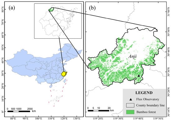
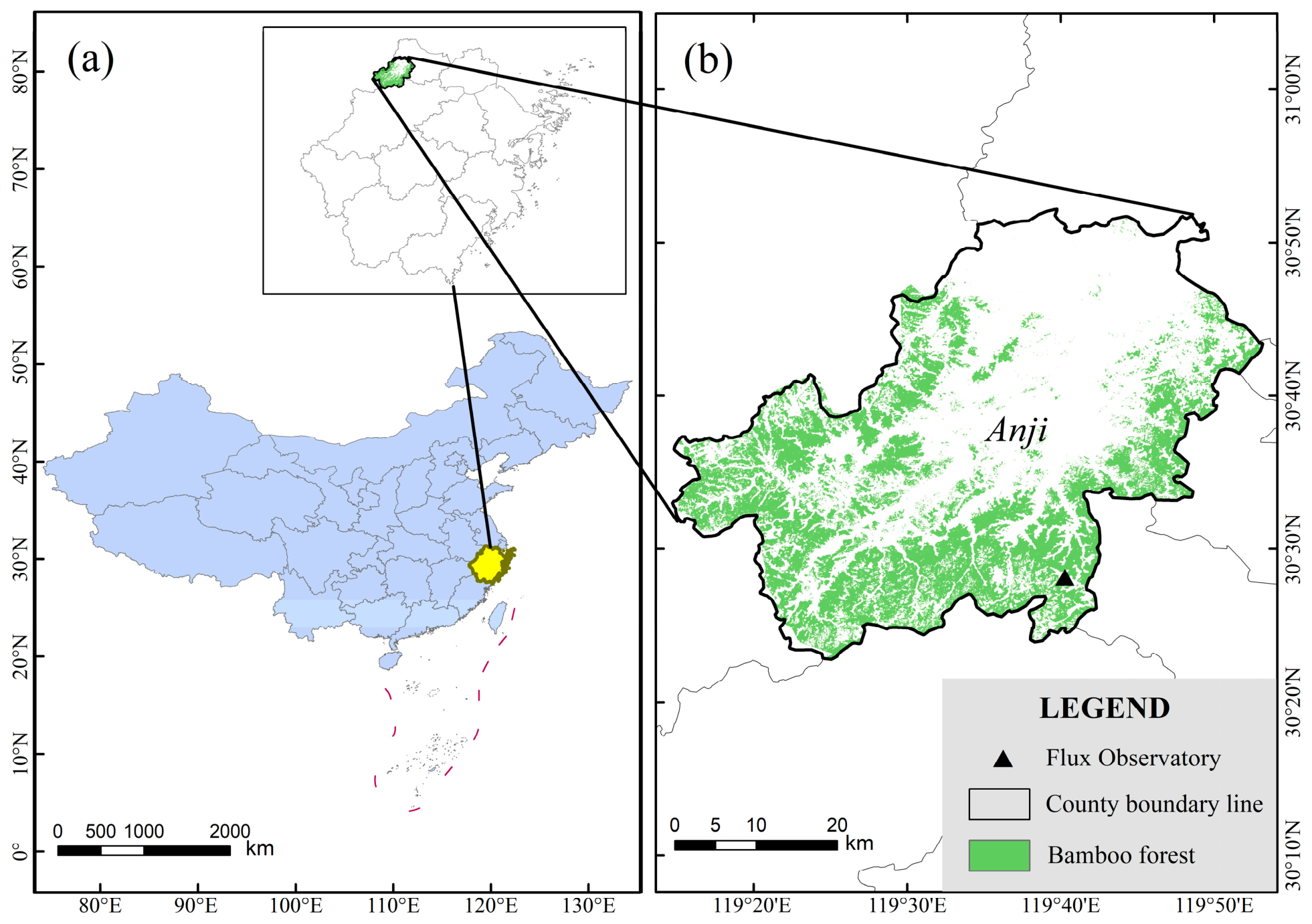
Anji County is located in northwestern Zhejiang Province, China (119°14′–119°53′ E, 30°23′–30°53′ N), covering a total area of 1886 km2 (Figure 1). The county has an elevation range of approximately 19–1423 m above sea level, and the mapped Moso bamboo area used in this study covers approximately 646 km2. The terrain is a dustpan-shaped basin surrounded by mountains on three sides, with elevation gradually decreasing from the southwest to the northeast. Mountainous areas dominate the southern, eastern and western parts; rolling hills lie in the central region, terraced land is distributed in the north, and flat plains are located along the Xitiao River. This region has a northern subtropical monsoon climate. The annual mean temperature is 16.6 °C, annual total precipitation reaches 1400 mm, with approximately 143 rainy days and 2021 h of sunshine per year [27]. The vegetation coverage exceeds 70%, and Anji is widely known as the “Hometown of Bamboo” for its abundant Moso bamboo resources, and previous studies have demonstrated the feasibility of mapping bamboo forests using multi-source remote sensing data [31].
Figure 1.
Location of study area and the single flux observation station. (a) Location of Anji County in eastern China; (b) mapped Moso bamboo distribution and tower location within Anji County.
2.2. Flux Data
The bamboo forest flux observation station is situated at 30.46° N, 119.66° E with an elevation of 380 m (Figure 1b). It was built in late 2010 within a subtropical maritime monsoon zone, and the surrounding area within a 1 km radius is dominated by intensively managed Moso bamboo stands [27]. The investigated Moso bamboo forest has a mean culm height of approximately 11 m, an average diameter at breast height of 9.3 cm and a stand density of 3235 stems per hectare [10,27]. It exhibits a biennial growth cycle, with vigorous growth in odd-numbered years and reduced growth in even-numbered years. The growing season ranges from April to November, including the rapid growth stage (April–May), main growth stage (June–September) and late growth stage (October–November) [6].
Eddy covariance (EC) systems were deployed to continuously measure CO2 fluxes. The system consists of an open-path infrared CO2/H2O gas analyzer (LI-7500, LI-COR Biosciences, Inc., Lincoln, NE, USA) and a three-dimensional sonic anemometer (CSAT3, Campbell Scientific, Inc., Logan, UT, USA), mounted at roughly three times the canopy height. Flux data were recorded by a CR1000 data logger (Campbell Scientific, Inc., Logan, UT, USA) at a sampling frequency of 10 Hz [10]. In this study, the monthly net ecosystem exchange (NEE) data from January 2011 to December 2015 were obtained from the published literature [10]. The monthly flux values were digitized from the original figures using WebPlotDigitizer-4.7, an open-source tool for extracting numerical data from scientific plots. The extracted NEE data were then converted to net ecosystem production (NEP = −NEE) and used as the target variable for developing and evaluating the monthly NEP prediction models; RF was selected for the regional reconstruction.
2.3. Geospatial Data
The integration of multi-source remote sensing data with machine learning has emerged as a powerful approach for ecosystem flux upscaling [32]. We collected multi-source meteorological and remote sensing datasets to drive the NEP prediction model. Meteorological variables included air temperature (TA), precipitation (PREC), solar radiation (SRAD) and vapor pressure deficit (VPD). TA, PREC, and SRAD were derived from the China Meteorological Forcing Dataset version 2.0 (CMFD v2.0) at a spatial resolution of 0.1° [33,34]. VPD was calculated based on ERA5-Land reanalysis data from the European Centre for Medium-Range Weather Forecasts (ECMWF) [35], following the method proposed by Yuan et al. [36]. All meteorological data were interpolated to 500 m resolution using bilinear interpolation [37].
Vegetation remote sensing indicators, including the Normalized Difference Vegetation Index (NDVI), Leaf Area Index (LAI) and Fraction of Absorbed Photosynthetically Active Radiation (FAPAR), were obtained from the Global Land Surface Satellite (GLASS) dataset [38]. The original 8-day GLASS products were aggregated to monthly composites using temporal weighted averaging based on the overlap between 8-day intervals and each calendar month. Solar-induced chlorophyll fluorescence (SIF) data were acquired from the China National Solar-induced Fluorescence (CNSIF) dataset with a 500 m resolution for the period 2003–2022 [39].
The bamboo forest mask was resampled from 30 m to 500 m using the nearest neighbor method. The 30 m bamboo classification was aggregated to the common 500 m grid by assigning each output-cell class from the nearest source-cell center, preserving categorical labels and avoiding interpolation-created fractional classes. This static nearest-neighbor mask provides a consistent spatial support for the 2003–2022 reconstruction but cannot represent within-cell bamboo fraction or land-cover change. All datasets were finally aligned to a unified 500 m grid and clipped to the administrative boundary of Anji County.
Detailed information on all input variables is summarized in Table 1.
Table 1.
Model predictor variables and data sources.
2.4. Model Construction and Evaluation
A data-driven model was established to upscale bamboo fluxes from the site-scale to the regional scale based on an automated machine-learning framework—Fast and Lightweight AutoML Library (FLAML). It performs model selection and hyperparameter optimization under a specified computational budget [20,24,25,40,41,42]. We used it to compare five candidate regression algorithms for monthly NEP prediction.
The calibration dataset comprised 60 monthly observations from January 2011 through December 2015. Samples were ordered chronologically: the first 48 months (January 2011–December 2014; 80%) formed the training set, and the final 12 months (January–December 2015; 20%) were retained as a temporal holdout test set. Within the 48-month training period, five-fold time-series cross-validation was used for hyperparameter tuning, with each validation block occurring after its corresponding training block. Five candidate models were evaluated—XGBoost, xgb_limitdepth, CatBoost, Random Forest (RF), and Extra Trees—using R2 as the optimization metric.
Model performance was evaluated using the coefficient of determination (R2), root mean squared error (RMSE), and mean absolute error (MAE), following established data-driven flux-model evaluation practice [17,20,23,24,25]. RF provided the best performance among the five candidates, with R2 values of 0.66 for the training set and 0.65 for the 12-month temporal holdout set (RMSE = 14.33 g C m−2 month−1; Figure S1; Table S1). RF was therefore selected as the final prediction model and applied to the monthly predictor fields to reconstruct NEP across the mapped Moso bamboo area from January 2003 to December 2022. Robustness was evaluated through the chronological holdout, the five-algorithm comparison, and external consistency checks against published site-, county-, and province-scale estimates discussed in Section 4.1. Because no additional independent bamboo-flux tower was available, these comparisons assess temporal robustness and consistency rather than independent spatial validation.
2.5. Technical Workflow and Analysis Methods
2.5.1. Theil–Sen Trend Estimation
The Theil–Sen estimator, also referred to as Sen’s slope, is a classic non-parametric method for time series trend analysis [43]. This approach is robust to outliers and has been widely applied to detect long-term dynamics of vegetation and ecological indicators [44,45]. In this study, we adopted the Theil–Sen approach to calculate the interannual variation rate of net ecosystem production (NEP) and all driving factors at the pixel scale. The calculation formula is as follows:
where β refers to the interannual trend slope of the target variable; xi and xj represent the values of time series in the i-th and j-th year, respectively. A positive β indicates an upward trend, while a negative β represents a downward trend.
2.5.2. Mann–Kendall Significance Test
The Mann–Kendall (MK) non-parametric test was used to examine the statistical significance of trends derived from the Theil–Sen estimator [46,47]. This method requires no normal distribution of raw data and is insensitive to abnormal values. The relevant formulas are presented below:
A trend is statistically significant at the 95% confidence level when ∣Z∣ ≥ 1.96. The county-total trend line was estimated with Theil–Sen, whereas its reported R2 and slope p-value were obtained from a separate ordinary least-squares regression. For pixel-level sensitivity analysis, raw p-values were additionally adjusted using the Benjamini–Hochberg procedure. Spatial dependence and possible temporal autocorrelation were not removed by this adjustment; pixel fractions are descriptive summaries of the modeled map.
2.5.3. RF-SHAP Attribution Framework
RF was adopted for regression modeling in this study [48]. To interpret the models and quantify the contribution of each predictor, we employed SHAP [28,49]. SHAP is a game theory-based approach that quantifies the marginal contribution of each feature to model predictions by computing Shapley values. The absolute SHAP value reflects the influence magnitude of each variable, where positive and negative values indicate contributions above and below the model baseline, respectively. The integration of machine learning with SHAP has been successfully applied across various environmental studies [50,51,52].
The trend-scale RF-SHAP analysis used one observation per pixel: the response was the 2003–2022 Theil–Sen slope of modeled annual NEP, and the eight predictors were their corresponding pixel slopes (n = 2855 pixels with complete data and raw p < 0.05 for the modeled NEP trend). SHAP values were computed for all retained pixels and summarized by mean absolute value; Tree SHAP interaction values were summarized separately as diagonal main-effect and off-diagonal pairwise allocations. The annual-scale RF-SHAP analysis used 59,540 pixel-year observations (2977 pixels × 20 years), with modeled annual NEP as the response and annual predictor values as inputs. Annual mean SHAP values were obtained by averaging each predictor’s SHAP values across pixels within each calendar year. Zero crossings of smoothed dependence curves indicate changes relative to an RF baseline.
To evaluate the relative importance of meteorological versus vegetation variables, we compared two modeling scenarios using a Random Forest model trained on the full dataset: (1) meteorological factors only, and (2) meteorological factors combined with vegetation remote sensing indicators (Figure S2). When vegetation indices were excluded, air temperature (TA) was the dominant predictor. In contrast, when vegetation indices were included, NDVI emerged as the most influential variable, underscoring the critical role of canopy vegetation status in NEP prediction.
2.5.4. Structural Equation Modeling
To further explore direct and indirect pathways of association among multiple variables, we applied SEM [53,54]. The combination of Random Forest and SEM has been successfully employed to quantify the effects of biotic and abiotic factors on CO2 fluxes at multiple temporal scales [55]. In the SEM framework, meteorological factors were set as exogenous variables, vegetation indices served as intermediate endogenous variables, and annual NEP was defined as the final dependent variable. The general recursive structure was η = Bη + Γξ + ζ, where ξ denotes the exogenous meteorological trends, η contains the endogenous vegetation-index and NEP trends, B and Γ are path-coefficient matrices, and ζ denotes residual errors. Standardized indirect associations were calculated as products of the component paths. The exploratory SEM used 2855 pixel-level trends selected from areas with significant modeled NEP trends (raw p < 0.05).
Four common fitness indices were used to evaluate model performance: Comparative Fit Index (CFI), Goodness-of-Fit Index (GFI), Root Mean Square Error of Approximation (RMSEA) and Standardized Root Mean Square Residual (SRMR). The model was regarded as well-fitted when CFI > 0.90, GFI > 0.90, RMSEA < 0.08 and SRMR < 0.05. All SEM calculations were implemented in R 4.4.1 using the lavaan package (version 0.6-21) [56]; sem(), parameterEstimates(), and fitMeasures() were used for fitting, standardized coefficients, and model-fit indices, respectively.
3. Results
3.1. Spatial Patterns and Seasonal Cycles of Bamboo Forest NEP in Anji County
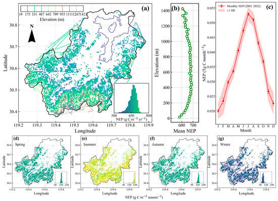
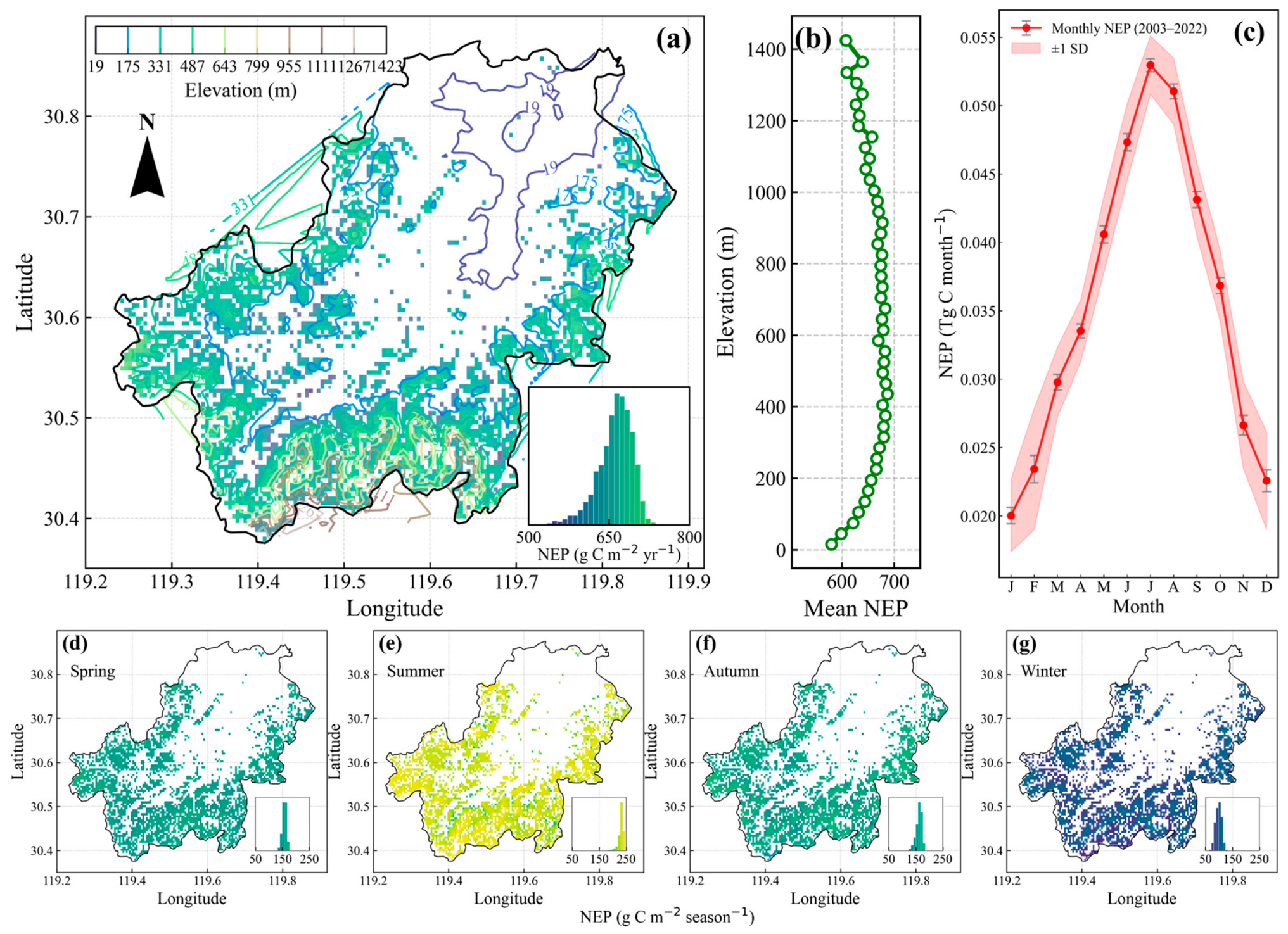
This section characterizes the multi-year mean spatial distribution and seasonal dynamics of net ecosystem production (NEP) across Anji’s bamboo forests from 2003 to 2022. The regional averaged NEP reached 665.69 ± 32.04 g C m−2 yr−1, with a coefficient of variation (CV) of only 0.05, indicating weak overall spatial heterogeneity across the study area (Figure 2a,b). A weak but statistically significant correlation was detected between NEP and elevation (r = 0.22, R2 = 0.05, p < 0.001), following a distinct unimodal pattern: NEP peaked at mid-elevations (342–550 m, 681.45 ± 25.44 g C m−2 yr−1) and slightly decreased at elevations above 550 m (671.41 ± 23.82 g C m−2). In addition, the standard deviation of NEP declined with increasing elevation (32.38 for low elevations vs. 23.82 for high elevations), suggesting more homogeneous carbon sequestration capacity at high-elevation bamboo stands.
Figure 2.
Spatial distribution and seasonal variation in multi-year averaged NEP (2003–2022) in Anji bamboo forests. (a) Spatial pattern of annual mean NEP; (b) elevation distribution of annual mean NEP; (c) monthly variation in total NEP; (d–g) seasonal spatial patterns of NEP in spring, summer, autumn, and winter, respectively.
In contrast to mild spatial variation, bamboo NEP exhibited strong seasonal fluctuations (Figure 2c). Monthly total NEP increased from 20 Gg C in January to the annual peak of 53 Gg C in July, and gradually declined to 23 Gg C in December, forming a typical summer peak and winter trough pattern consistent with bamboo phenology (Figures S3 and S4 further reveal that monthly NEP showed synchronous unimodal seasonal cycles with most environmental drivers and significant positive seasonal correlations with nearly all climate and vegetation factors except precipitation). Summer (June–August) contributed 35.4% of the annual total carbon sequestration, ranking the highest among four seasons.
Across all seasons, however, spatial patterns remain highly uniform (Figure 2d–g). Spring NEP is moderate (134–181 g C m−2 season−1), rising sharply in summer (182–246 g C m−2 season−1) with contiguous distribution across the region, then declining in autumn and reaching the annual minimum in winter (73–134 g C m−2 season−1). Within each season, NEP differences among elevation zones are less than 2 g C m−2 season−1, and spatial CV is below 0.11, with no persistently high-value core area. Consequently, the large seasonal amplitude (summer exceeds winter by ~130 g C m−2 season−1) is driven by seasonal factors, not by spatial location or topography.
3.2. Long-Term Dynamics of Bamboo Forest NEP in Anji County over 2003–2022
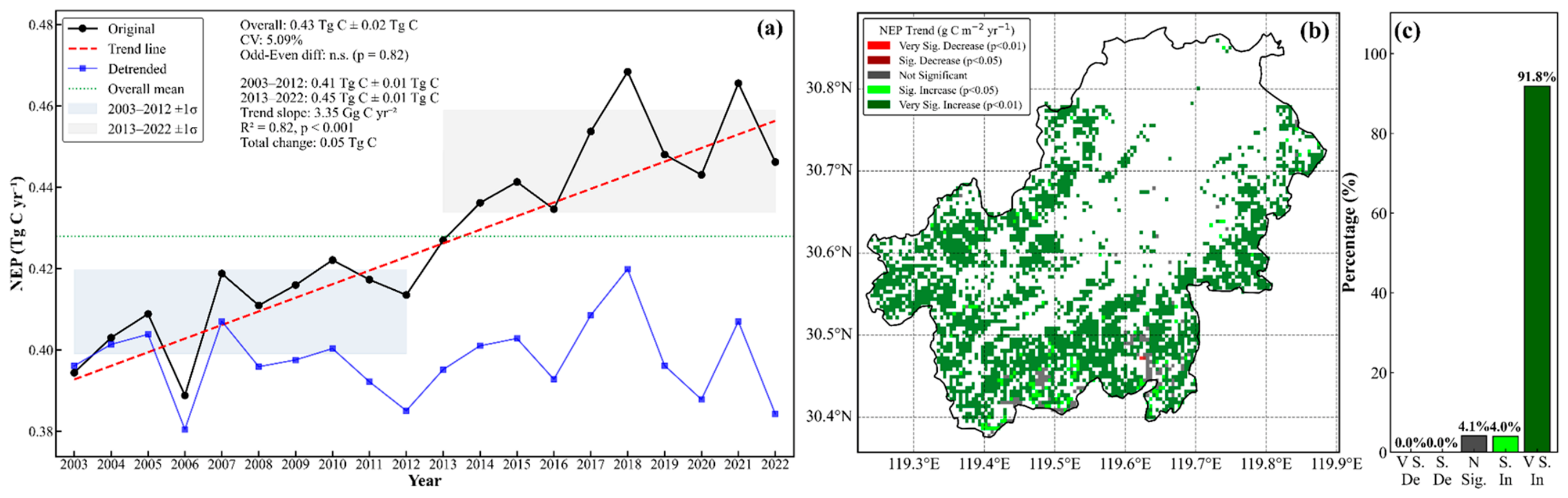
Over the 20-year study period, the annual total NEP of Anji bamboo forests averaged 0.43 ± 0.02 Tg C yr−1 (range: 0.39–0.47 Tg C yr−1), with a low interannual CV of 5.09%, indicating stable annual carbon sequestration (Figure 3a). The modeled product showed a significant increasing trend (Theil–Sen slope = 3.35 Gg C yr−2, R2 = 0.82, p < 0.001), corresponding to a 13.13% increase from 2003 to 2022.
Figure 3.
Long-term interannual variation and spatial trends of NEP in Anji bamboo forests (2003–2022). (a) Interannual dynamics of annual total NEP and phase division; (b) spatial distribution of NEP long-term trends; (c) percentage statistics of trend significance grades.
Several modeled NEP anomalies occurred in 2006, 2012–2013, 2019–2020 and 2022, which coincided with extreme high temperature and drought events across southern China [57]. To explore the responses of carbon sinks to climate extremes, we detrended the long-term NEP time series and selected two representative drought years (2006 and 2022) for comparative analysis (see spatial and seasonal patterns in Figures S5–S8). In 2006, persistent precipitation deficits suppressed vegetation growth across most regions, and 50.4% of bamboo pixels showed slight NEP decline. Differently, 2022 experienced a humid and favorable spring that boosted early carbon uptake, while severe compound summer drought mainly restricted NEP in central and northern low hills. Only 46.2% of the study area exhibited slight NEP reduction, leading to a milder annual carbon loss compared with 2006.
We further examined the influence of the biennial growth cycle of Moso bamboo. It is important to note that the timing of the biennial on/off cycle varies spatially depending on stand age, management history, and local harvest schedules [10]. Different bamboo stands within Anji County may be in opposite phases of the cycle at any given year, leading to spatial averaging at the regional scale. Consistent with this expectation, we found no statistically significant difference in mean annual NEP between odd and even years at the county level (odd years: 0.4297 ± 0.0212 Tg C yr−1; even years: 0.4273 ± 0.0223; p = 0.82). This finding does not imply the absence of biennial cycles at the plot scale; rather, it reflects that spatial heterogeneity in harvest timing smooths out the biennial pattern when aggregated to the county level.
Spatially, the long-term increasing trend of NEP was widespread across the entire bamboo area (Figure 3b,c). Among all bamboo pixels, 91.8% showed a very significant increasing trend (p < 0.01), and another 4.0% presented a significant increase (p < 0.05); the total proportion of rising areas reached 95.8%. Pixels with non-significant changes accounted for 4.1%, while declining pixels were negligible (only 2 pixels, 0.1%). Spatially, the increasing rate of NEP was higher in the western and eastern bamboo zones, and relatively weaker in the central-eastern belt (119.6–119.7° E), where scattered declining pixels were exclusively distributed.
3.3. Model-Based Attribution of Long-Term NEP Variation in Anji County
We used RF-SHAP analyses at trend and annual scales, together with exploratory SEM, to characterize contributions of environmental covariates and statistical pathways associated with the 13.13% increase in modeled NEP.
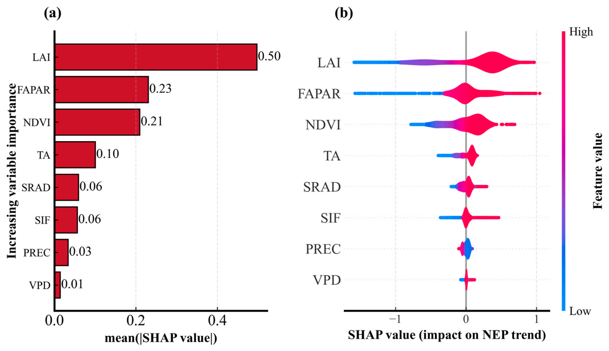
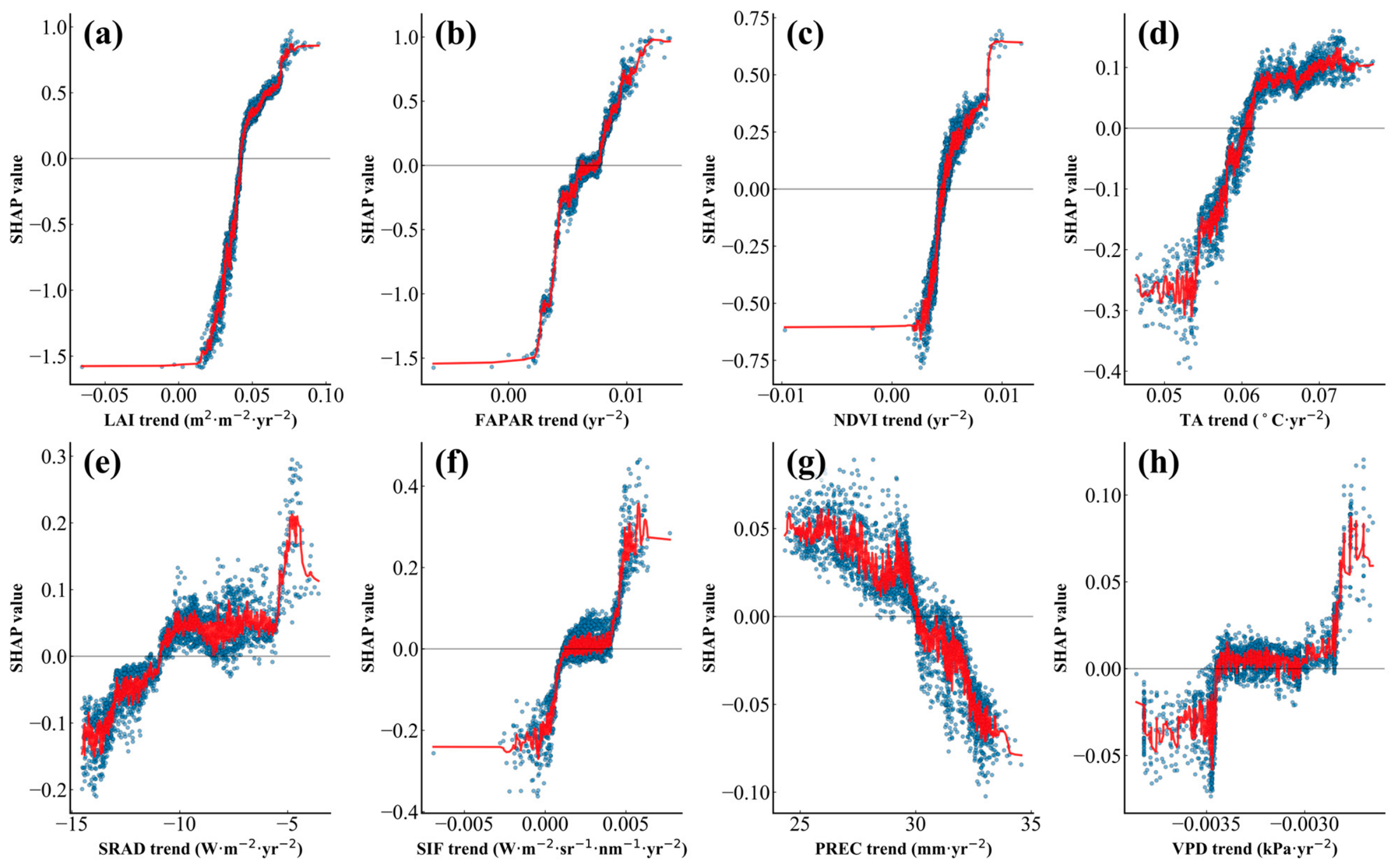
At the trend scale, LAI, FAPAR, and NDVI had the three largest mean absolute SHAP values, followed by TA, SRAD, SIF, PREC, and VPD (Figure 4a). In the SHAP beeswarm plot (Figure 4b), higher trend values in the vegetation indices corresponded to positive model contributions, whereas lower values corresponded to negative contributions. The smoothed dependence curves showed nonlinear sign changes within the observed ranges (Figure 5a–h). For LAI, FAPAR, NDVI, TA, and SIF, model-attributed contributions generally shifted from negative to positive as the trend values increased, whereas increasing PREC trends were associated with negative contributions. Stronger declines in SRAD were associated with more negative contributions, and VPD contributions remained near zero over most of its observed range.
Figure 4.
SHAP-based variable importance for environmental covariates of long-term NEP trends. (a) Mean absolute SHAP values; (b) SHAP beeswarm plot showing signed environmental covariates contributions. Blue and red indicate low and high covariate-trend values, respectively; positive and negative SHAP values denote model contributions above and below the model baseline.
Figure 5.
SHAP dependence plots for eight environmental covariates trends. Subplots (a–h) correspond to LAI, FAPAR, NDVI, TA, SRAD, SIF, PREC, and VPD. Blue dots represent pixel samples, red smoothed lines summarize nonlinear model responses, and the horizontal line marks a SHAP value of zero.
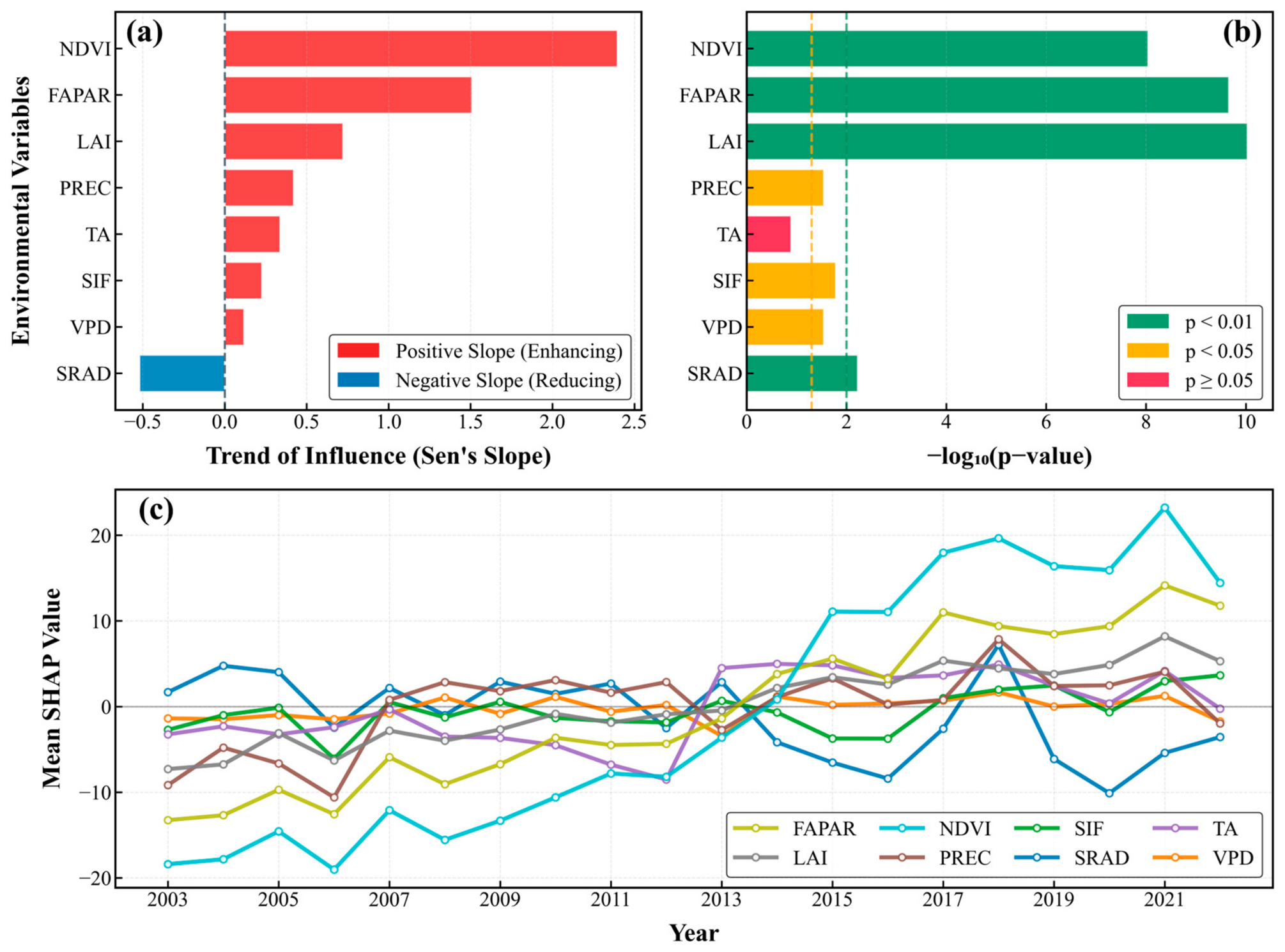
Theil–Sen slopes and Kendall’s tau tests applied to annual mean SHAP values showed increasing contributions for seven of the eight environmental covariates, whereas the contribution of SRAD decreased (Figure 6a–c). NDVI and FAPAR had the steepest increases, and LAI, FAPAR, and NDVI showed significant upward trends (p < 0.01). SRAD had the largest annual mean model contribution before approximately 2013, whereas LAI, NDVI, and FAPAR had larger contributions thereafter.
Figure 6.
Long-term dynamics of annual mean SHAP contributions (2003–2022). (a) Trend magnitudes; (b) statistical significance of trends; (c) interannual variation in model-attributed environmental covariates contributions.
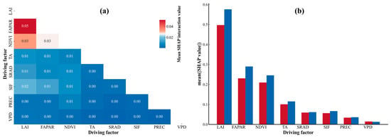
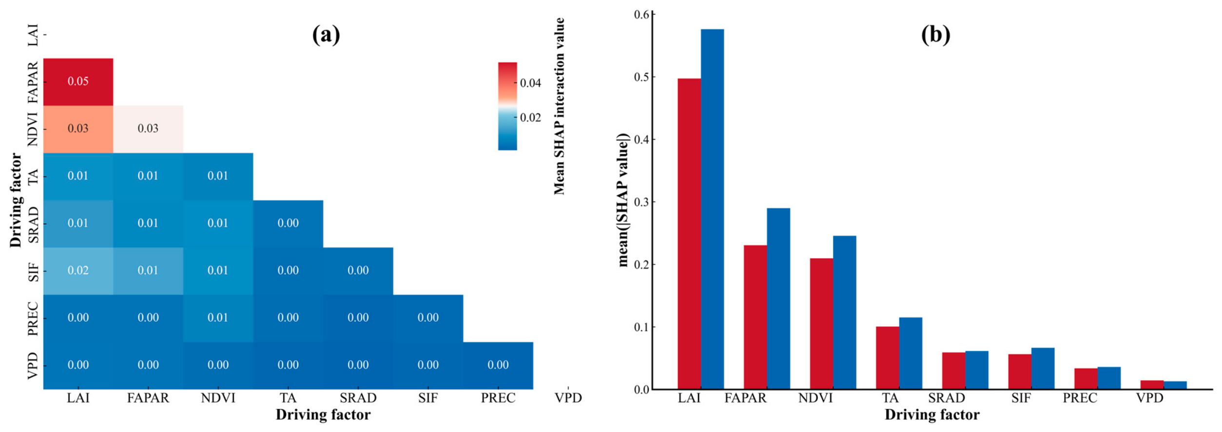
SHAP interaction values were largest among the canopy vegetation indicators (Figure 7a,b). The largest mean absolute interaction value was observed for LAI–FAPAR (0.05), followed by LAI–NDVI (0.03) and FAPAR–NDVI (0.03). The next strongest interactions involved LAI–SIF, FAPAR–SIF, and LAI–SRAD, whereas most remaining pairs were below 0.01. Thus, the strongest modeled interactions were concentrated among canopy-related factors. For LAI, FAPAR, and NDVI, the summed interaction contributions were slightly larger than their individual main effects, whereas both main and interaction contributions were small for the meteorological factors. The pairwise SHAP interaction plots showed structured nonlinear patterns among LAI, FAPAR, and NDVI, whereas interactions involving TA were weaker (Figure S9).
Figure 7.
SHAP interaction contributions of all driving factors. (a) Lower-triangle heatmap of mean absolute SHAP interaction values; red represents strong coupling and blue denotes weak interactions. (b) Grouped bar plot comparing individual main effects (red) and total cross-factor interaction contributions (blue).
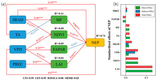
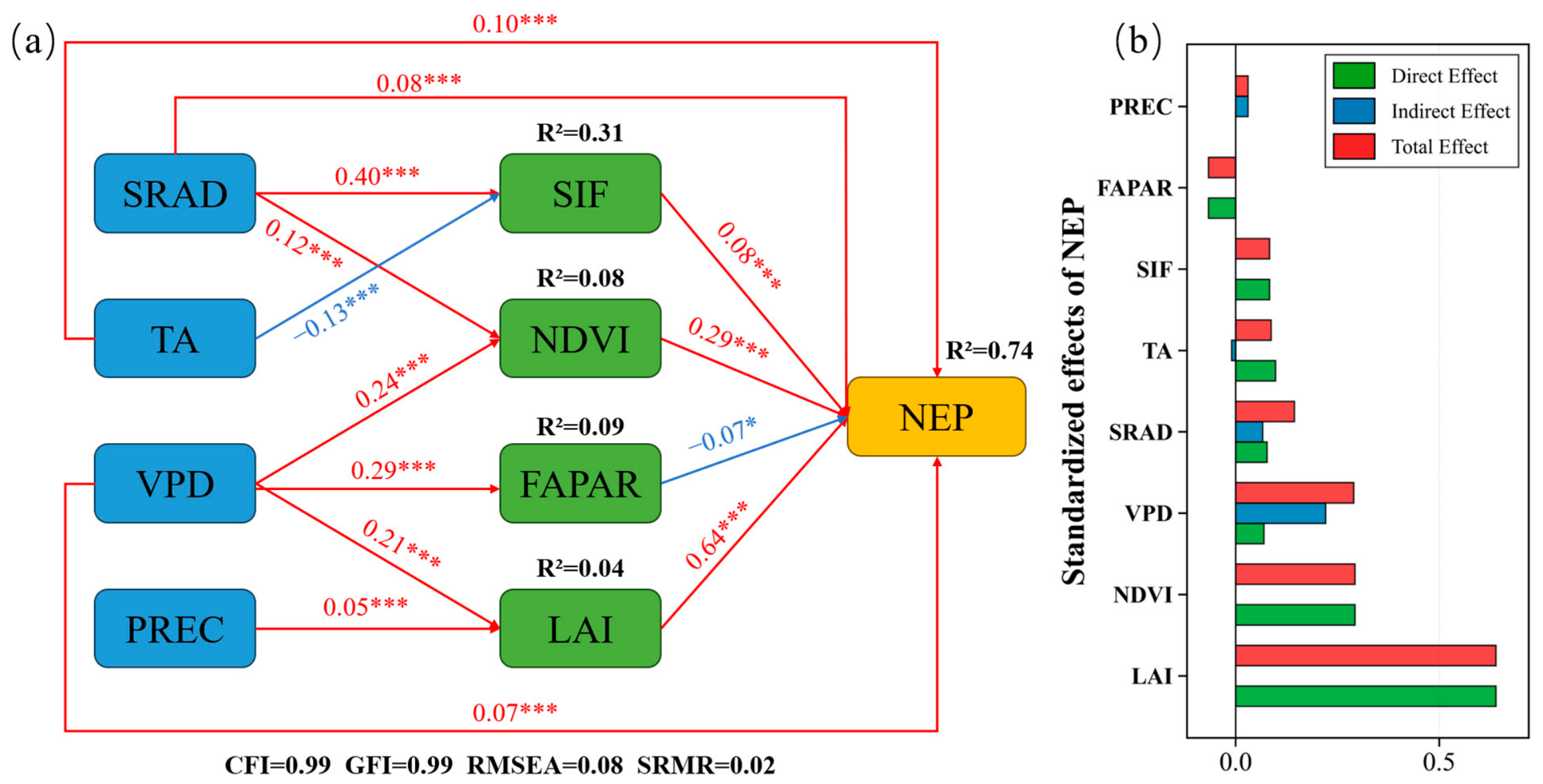
The exploratory SEM used 2855 pixels with significant modeled NEP trends and ac-counted for 74% of the variance in modeled NEP trends (R2 = 0.74); global fit indices are reported in Figure 8 and were considered jointly (Figure 8a,b). LAI trend had the largest standardized positive association with modeled NEP trend (coefficient = 0.64, p < 0.001). Direct path coefficients from meteorological variable trends to NEP trend were small, whereas paths connecting meteorological variable trends to vegetation index trends and vegetation index trends to NEP trend contributed more strongly to the modeled indirect associations. VPD, SRAD, and PREC trends had positive path coefficients to the four canopy index trends, while TA trend had a weak negative coefficient to SIF trend. R2 values for the vegetation mediators were lower (SIF 0.31, NDVI 0.08, FAPAR 0.09, LAI 0.04), indicating that the four meteorological trends represented only a limited fraction of their spatial variability. The reported paths summarize covariance among variables, including a modeled response.
Figure 8.
Exploratory SEM of statistical associations among interannual trends of climate variables, vegetation indicators, and modeled NEP. (a) Standardized path coefficients; red and blue lines indicate significant positive and negative associations, respectively. R2 values for each endogenous variable and global fit indices are annotated. (b) Decomposition of standardized direct, indirect, and total associations with modeled NEP trends. * p < 0.05; *** p < 0.001.
Across the model-based attribution analyses, vegetation variables had larger contributions than meteorological factors, and the annual ranking of predictor contributions changed around 2013. The ecological interpretation and limitations of these statistical patterns are considered in the Discussion.
4. Discussion
4.1. Evaluation and Scope of the Regional NEP Estimates
The chronological 2015 holdout (R2 = 0.65) and 11 post-calibration months in 2016 (prediction R2 = 0.41; Pearson’s r = 0.73, p = 0.01; Table S1; Figures S1 and S11) indicate temporal predictive skill at the calibration footprint. However, the 2016 predictions compressed the seasonal amplitude (regression slope = 0.31): RMSE was 30.16 g C m−2 month−1 (57.8% of the observed monthly mean), MAE was 26.35 g C m−2 month−1, and mean bias was +7.66 g C m−2 month−1. The 2016 observations were excluded from model selection and recalibration, which making this a temporal test; satellite-based driver products do not by themselves ensure independence. Because both evaluations use the same tower footprint, neither establishes spatial transfer to stands differing in age or management. Grid–footprint mismatch may also contribute to the 2016 errors.
Prior work offers useful context rather than a direct performance benchmark. Mao et al. used LAI assimilation with the process-based BEPS model to estimate bamboo carbon fluxes across Zhejiang Province [14], while an improved BIOME-BGC model represented bamboo phenology, carbon allocation, and management at a monitored stand [15]. Our RF combines multiple meteorological and satellite predictors to reconstruct monthly NEP but does not explicitly resolve stand age, harvest, or other management. Because the studies differ in flux target, temporal scale, spatial support, and evaluation design, their reported R2 values cannot establish that the present RF is more accurate.
Spatial context also matters. The estimated 0.43 Tg C yr−1 for approximately 646 km2 of mapped Anji bamboo corresponds to approximately 6.66 Mg C ha−1 yr−1; Mao et al. reported 1.74 Tg C yr−1 for bamboo forests across Zhejiang Province [14]. These totals refer to different domains and methods and should not be treated as directly comparable or as independent validation. Inventory-based carbon-stock changes and EC-derived NEP represent different quantities, so their difference cannot be attributed solely to belowground carbon [58,59]. The main contribution of the present product is a consistent monthly 500 m grid description of where and when modeled NEP varies over 2003–2022, which can prioritize additional flux measurements and management-stratified tests. It does not establish the effects of a particular management intervention.
Negative modeled NEP anomalies in 2006 and 2022 coincided with low rainfall in the input data; the severe 2022 Yangtze River Basin drought has also been independently documented [57]. Both years lie outside the available flux-observation period. This agreement cannot independently validate the magnitude or cause of those anomalies.
4.2. Drivers of the Long-Term NEP Increase and Implications for Management
Within the fitted models, LAI, NDVI, and FAPAR made the largest contributions to predicted NEP, although their ranking differed between trend and annual analyses. This result is plausible because these indices integrate canopy amount, phenology, and photosynthetic condition more directly than coarse meteorological fields. It should nevertheless be interpreted cautiously: the vegetation indices are correlated, and both SHAP and SEM partition associations among variables that were also used to generate the NEP estimates. The negative direct FAPAR coefficient in the SEM, despite its high SHAP importance, further illustrates that individual paths need not represent independent physiological effects. The trend-scale and annual-scale attribution RFs explain a regional product generated by the tower-trained RF; predictor reuse means this is an analysis of model behavior, not independent confirmation of environmental controls.
The descriptive crossover around 2013 coincided with diverging predictor trajectories. Solar radiation declined over the study period (slope = −10.65 W m−2 yr−1, R2 = 0.47, p < 0.001; Figure S10a). Other climate trends and their spatial associations with NEP are summarized in Figure S10b–h; NDVI, FAPAR, and LAI increased strongly (R2 > 0.91; Figure S10i,j,l). As the vegetation indicators moved farther from the model baseline, their mean SHAP contributions increased and exceeded that of SRAD. This pattern provides a statistical explanation for the changing model attribution, but it does not by itself demonstrate an abrupt ecological regime shift.
Several processes could have contributed to the post-2013 greening signal. China’s ecological-civilization and forest-conservation policies intensified after 2012 [60,61], management may have altered stand density and canopy condition, and warming may have lengthened the subtropical growing season [62]. Similar changes in the relative importance of climatic and vegetation indicators have been reported in other forest regions [63,64]. However, long-term stand-management records were unavailable here, so the respective roles of policy, management, CO2 fertilization, and climate cannot be separated. Future work should pair flux measurements with stand age, harvest, fertilization, and disturbance records.
No significant county-scale difference was detected between odd- and even-year modeled NEP. This absence of a regional parity signal does not show that the biennial growth cycle has no ecological effect. Plot-scale studies have documented harvest-related interannual variability [10], but asynchronous stand ages and harvest schedules can weaken a county-wide signal. Management data resolved by stand and year are needed to test this explanation directly.
The comparatively low R2 values for the vegetation mediators in Figure 8a indicate that the specified meteorological trends explained only a limited share of spatial variation in SIF, NDVI, FAPAR, and LAI trends. This is expected because canopy dynamics also depend on stand age, stand density, harvest and fertilization history, soil moisture and nutrients, topography, and scale mismatch or measurement error, none of which was represented fully in the SEM. These mediator R2 values describe explained variance within the exploratory path model; they are not the predictive-validation R2 of the RF NEP model and do not invalidate the relatively high R2 for modeled NEP trend.
The SEM identified statistical pathways linking climate variables, canopy condition, and modeled NEP. Positive path coefficients for SRAD, TA, and PREC and a negative coefficient for VPD (Figure S10) are broadly consistent with the sensitivity of subtropical vegetation to energy and atmospheric moisture demand [65,66]. Nevertheless, meteorological inputs were spatially coarser than the 500 m output grid, and the apparent indirect pathways should be evaluated with additional flux sites or process-based counterfactual experiments.
The zero crossings in the SHAP dependence plots show where the fitted model contribution changes sign relative to its baseline; they should not be interpreted as physiological thresholds. Even so, the combined patterns suggest that maintaining canopy condition may help sustain carbon uptake. Because correlated greenness indices can respond simultaneously to climate and management, field measurements are required to identify which canopy properties are most actionable.
For management, the results support continued monitoring of canopy condition together with stand age, harvest intensity, and drought exposure. The contrasting modeled anomalies in 2006 and 2022 suggest that seasonal precipitation deficits and high atmospheric demand may temporarily offset gains associated with greening [57]. Testable management options include maintaining moderate stand density, staggering harvests among stands, conserving soil moisture, and avoiding intensive harvesting during drought-prone periods. Under future warming, strategies that maintain stand vigor while reducing drought vulnerability may therefore be more robust than maximizing canopy density alone. These implications should be tested through management experiments and expanded flux observations.
Overall, the analysis indicates a strengthening modeled carbon sink and a growing contribution of vegetation condition factors, but it does not uniquely attribute that change to climate or management. The main value of the product is to identify spatial and temporal patterns that can guide field validation and targeted monitoring.
4.3. Limitations and Outlook
This study has several limitations. First, model development used 60 monthly observations from a single eddy-covariance tower during 2011–2015. The chronological 2015 holdout assesses temporal prediction at that site, but not spatial transferability. Extrapolation across 2003–2022 and among bamboo stands therefore assumes that the fitted relationships remain sufficiently stable; low mapped heterogeneity and agreement with published estimates provide consistency checks, not proof of regional validity. Likewise, modeled anomalies in 2006 and 2022 coincide with known droughts but do not constitute independent flux validation. Second, a static bamboo map cannot represent expansion or conversion over two decades, and time-varying vegetation indices do not fully correct land-cover classification error. Third, harvesting, fertilization, stand age, and other management disturbances were unavailable, limiting interpretation of the county-scale odd–even comparison and the post-2013 greening signal [2]. Additional uncertainty arises from digitized flux targets, forcing products, RF fitting, static-mask classification, and spatial and temporal transfer; these components have not been combined into calibrated predictive intervals. Trend tests and SEM p-values do not account fully for spatiotemporal dependence. The trend-scale attribution sample was selected using modeled-NEP significance, so its associations are conditional on that selected subset rather than representative of all pixels.
In future research, we will integrate dynamic land cover data, stand age, stand density, harvest, and fertilization records, and local soil moisture, soil nutrients, and topographic variables to optimize the model. We also plan to combine process-based models with interpretable machine learning to improve the physical interpretability and extrapolation ability of carbon flux simulation [19,67]. Expanding the eddy covariance network to include multiple bamboo stands would also help constrain model parameters.
Within these limitations, the Anji results provide a model-based assessment in which vegetation greenness—potentially reflecting both climate variability and management—was most strongly associated with the long-term increase in predicted carbon uptake. Expanded flux observations and management records are required before extending this interpretation to subtropical bamboo forests more generally.
5. Conclusions
This study estimated monthly NEP on a 500 m grid for approximately 646 km2 of mapped Moso bamboo forests in Anji County from 2003 to 2022 by integrating single-site eddy-covariance observations, meteorological data, and multi-source remote-sensing products within an automated machine-learning framework.
Modeled bamboo NEP showed weak overall spatial heterogeneity but clear elevational and seasonal patterns, with the highest estimates at mid-elevations and in summer. Annual NEP increased significantly over the study period, and 95.8% of bamboo pixels showed upward trends. No county-scale odd–even signal was detected in annual modeled NEP, while negative anomalies coincided with major drought years.
We characterized regional NEP patterns and used SHAP and exploratory SEM to summarize contributions of environmental covariates and statistical associations. Within the fitted model, LAI, FAPAR, and NDVI made the largest contributions to long-term NEP variation. Their annual mean SHAP contributions exceeded that of solar radiation after approximately 2013, representing a descriptive change in model attribution. The exploratory SEM was consistent with statistical pathways linking meteorological variables, vegetation conditions, and modeled NEP. The greening signal may combine climate and management influences that cannot be separated with the available data.
Overall, this study reveals a long-term increase and shifting predictor contributions of NEP in subtropical Moso bamboo forests at the county scale. The regional reconstruction provides hypotheses and spatial information for targeted monitoring and future management experiments.
Supplementary Materials
The following supporting information can be downloaded at: https://www.mdpi.com/article/10.3390/f17101167/s1. Figure S1: Performance of the five candidate models evaluated within the FLAML framework. The models were CatBoost (a–c), Random Forest (RF) (d–f), XGBoost (g–i), xgb_limitdepth (j–l), and Extra Trees (extra_tree) (m–o). RF had the highest R2 on the chronological temporal holdout set. Figure S2: Exploratory SHAP variable importance ranking from preliminary site-level predictors screening. (a) uses locally available meteorological and soil variables; (b) adds vegetation remote-sensing variables. This exploratory screening is distinct from the final eight- predictors regional RF model summarized in Table 1 and is not an external validation. Figure S3: Intra-annual seasonal dynamics of monthly NEP and eight environmental driving factors in Anji bamboo forests. Red lines show NEP (right y-axis), and blue lines show each factor (left y-axis). NEP and the vegetation indices generally reached high values in June–July, whereas the timing and shape of the meteorological cycles differed among variables. Figure S4: Intra-annual seasonal linear correlations between monthly NEP and eight environmental factors in Anji bamboo forests. Presents monthly pairwise linear regression scatter plots. TA had the strongest significant positive seasonal correlation with NEP (r = 0.96, p < 0.01), followed by LAI (r = 0.95, p < 0.01). SRAD, FAPAR, SIF, NDVI and VPD also exhibited strong statistically significant positive correlations (all p < 0.01). Only monthly precipitation showed a weak non-significant correlation with seasonal NEP (r = 0.26, p > 0.05). Figure S5: Spatial pattern and area proportion of annual modeled NEP anomalies for bamboo forests in Anji in 2006. Anomalies are deviations of annual NEP from the 2003–2022 multi-year mean and are classified with a fixed 50 g C m−2 yr−1 magnitude threshold for spatial comparison. Slightly decreased bamboo areas accounted for 50.4% of the mapped domain and slightly increased for 49.3%; large decreases and large increases accounted for 0.1% and 0.2%, respectively. No pixel had an exact zero anomaly. The terms large and slight describe fixed magnitude classes, not statistical significance. Figure S6: Monthly anomalies of modeled NEP, vegetation indicators, and climate factors in Anji County in 2006. (a) Monthly total modeled NEP anomalies (Tg C month−1) were negative in most months, with a small positive anomaly in June. Vegetation indicators [(b) SIF, (c) LAI, (d) NDVI, and (e) FAPAR] were generally below their multi-year seasonal means during much of the growing season. Among the climate factors [(f) VPD, (g) SRAD, (h) TA, and (i) PREC], TA and SRAD showed temporary positive anomalies from late spring to summer, whereas PREC was below its seasonal mean during parts of spring and autumn. These parallel anomalies are consistent with, but do not independently demonstrate, a canopy- or drought-driven reduction in ecosystem carbon uptake. Figure S7: Spatial distribution and area proportion annual modeled NEP anomalies in Anji bamboo forests in 2022. Altitude contour lines are overlaid in subplot (a), and subplot (b) presents five fixed magnitude classes: slight increase (50.3%), slight decrease (46.2%), large decrease (2.3%), large increase (1.3%), and exact zero anomaly (0.0%). Compared with 2006, slight modeled NEP decreases were more common in the central and northern low hills, whereas increases were concentrated in southern high- altitude areas. The spatial pattern coincided with the documented 2022 Yangtze River Basin drought but does not independently establish its effect on NEP. Figure S8: Monthly anomalies of modeled NEP, vegetation indicators, and climate factors in Anji County in 2022. (a) Modeled NEP anomalies (Tg C month−1) were negative in January–February and July–November and positive in March–April and June. Vegetation indicators [(b) SIF, (c) LAI, (d) NDVI, and (e) FAPAR] were generally positive in spring and negative during much of summer and autumn. Among the climate factors [(f) VPD, (g) SRAD, (h) TA, and (i) PREC], PREC remained below its seasonal mean through much of spring–autumn, while SRAD, TA, and VPD had positive mid-summer anomalies. These concurrent model-input and output anomalies are consistent with the documented 2022 Yangtze River Basin drought but do not independently identify the cause or magnitude of the modeled NEP reduction. Figure S9: Pairwise SHAP interaction scatter plots for the top six canopy indicator combinations. Subplots (a–f) display SHAP interaction allocations against the trend gradient of the first predictor; point colour represents to the trend magnitude of the secondary predictor. The dashed zero line separates positive and negative model interaction allocations, not ecological synergy or antagonism. Figure S10: Interannual variations and spatial partial correlation patterns of climate and vegetation driving factors for bamboo forest NEP in Anji from 2003 to 2022. Time series subplots (a–d, i–l) depict regional annual means values and linear trend fits with 95% confidence bands, while spatial maps (e–h, m–p) show pixel-wise partial correlation coefficients with modeled NEP. NDVI, FAPAR and LAI exhibited significant positive long-term increasing trends throughout the study period. The bottom color bar quantifies partial correlation values ranging from −1.0 to 1.0. Figure S11: Same-site post-calibration independent temporal evaluation of the frozen RF model using 11 available monthly EC-based NEP observations from the same flux site in January–November 2016. (a) Observed and predicted monthly NEP; (b) predicted versus observed NEP. The dashed line indicates 1:1 agreement and the solid line is the ordinary least-squares regression. The 2016 observations were not used for model selection, hyperparameter tuning, or recalibration. December 2016 was unavailable and was not imputed. Prediction R2 = 0.41, RMSE = 30.16 g C m−2 month−1, MAE = 26.35 g C m−2 month−1, mean bias = +7.66 g C m−2 month−1, Pearson’s r = 0.73 (p = 0.01), and n = 11. This same-site test evaluates temporal generalization but not spatial transferability. Table S1: Candidate model performance on training and test sets.
Author Contributions
Conceptualization, W.H.; methodology, W.H., N.T.N. and P.X.; validation, Y.L. (Yanxia Li); formal analysis, X.L., W.H. and T.M.; investigation, W.H. and H.X., resources, S.F. and H.X.; data curation, X.L., Y.L. (Yanxia Li), M.Z., S.L. and Z.H.; writing—original draft preparation, X.L.; writing—review and editing, S.F., W.H., H.X., Y.L. (Yanxia Li), Y.L. (Yi Lin), J.C.T., S.M.-F., G.B., N.T.N., P.X., M.Z., S.L., T.M., Z.H. and J.K.; visualization, X.L.; supervision, S.F. and W.H.; project administration, S.F.; funding acquisition, S.F., W.H. and Y.L. (Yi Lin). All authors have read and agreed to the published version of the manuscript.
Funding
This research was funded by the National Natural Science Foundation of China (Grant No. 42277453 and 42407604), the Quadrature Climate Foundation (Grant No. 01-21-000133), and Huzhou Science and Technology Plan Project (Grant No. 2024GZ50).
Data Availability Statement
The raw data will be made available on the request.
Acknowledgments
We acknowledge Zhejiang A&F University for measuring and sharing the eddy covariance data. We sincerely acknowledge Jingfeng Xiao from New Hampshire University for providing the GOSIF data and Jianxi Huang from China Agricultural University for providing the CNSIF data. We sincerely thank Kun Yang from Tsinghua University for sharing the CMFD v2 meteorological reanalysis dataset. We also sincerely acknowledge Shunlin Liang’s group for sharing GLASS LAI, FAPAR, and NDVI data. We sincerely acknowledge Oksana Tarasova from World Meteorological Organization for reviewing our manuscript with constructive suggestions. During the preparation of this manuscript, we used DeepSeek (https://chat.deepseek.com/) and Grok (https://grok.com/) for the purposes of English language polishing. We reviewed and edited the output and take full responsibility for the content of this publication.
Conflicts of Interest
The authors declare no conflicts of interest.
References
- Pan, Y.; Birdsey, R.A.; Fang, J.; Houghton, R.; Kauppi, P.E.; Kurz, W.A.; Phillips, O.L.; Shvidenko, A.; Lewis, S.L.; Canadell, J.G.; et al. A Large and Persistent Carbon Sink in the World’s Forests. Science 2011, 333, 988–993. [Google Scholar] [CrossRef] [Scilit] [PubMed]
- Xu, L.; Shi, Y.; Zhou, G.; Xu, X.; Liu, E.; Zhou, Y.; Li, C.; Fang, H.; Deng, X. Temporal Change in Aboveground Culms Carbon Stocks in the Moso Bamboo Forests and Its Driving Factors in Zhejiang Province, China. Forests 2017, 8, 371. [Google Scholar] [CrossRef] [Scilit]
- Li, X.; Du, H.; Zhou, G.; Mao, F.; Zhu, D.; Zhang, M.; Xu, Y.; Zhou, L.; Huang, Z. Spatiotemporal patterns of remotely sensed phenology and their response to climate change and topography in subtropical bamboo forests during 2001-2017: A case study in Zhejiang Province, China. GISci. Remote Sens. 2023, 60, 2163575. [Google Scholar] [CrossRef] [Scilit]
- Chen, L.; Liu, Y.; Zhou, G.; Mao, F.; Du, H.; Xu, X.; Li, P.; Li, X. Diurnal and seasonal variations in carbon fluxes in bamboo forests during the growing season in Zhejiang province, China. J. For. Res. 2018, 30, 657–668. [Google Scholar] [CrossRef] [Scilit]
- Sun, J.; Mao, F.; Du, H.; Li, X.; Xu, C.; Zheng, Z.; Teng, X.; Ye, F.; Yang, N.; Huang, Z. Improving the Simulation Accuracy of the Net Ecosystem Productivity of Subtropical Forests in China: Sensitivity Analysis and Parameter Calibration Based on the BIOME-BGC Model. Forests 2024, 15, 552. [Google Scholar] [CrossRef] [Scilit]
- Xu, C.; Mao, F.; Du, H.; Li, X.; Sun, J.; Ye, F.; Zheng, Z.; Teng, X.; Yang, N. Full phenology cycle carbon flux dynamics and driving mechanism of Moso bamboo forest. Front. Plant Sci. 2024, 15, 1359265. [Google Scholar] [CrossRef] [Scilit] [PubMed]
- Kang, F.; Li, X.; Du, H.; Mao, F.; Zhou, G.; Xu, Y.; Huang, Z.; Ji, J.; Wang, J. Spatiotemporal Evolution of the Carbon Fluxes from Bamboo Forests and Their Response to Climate Change Based on a BEPS Model in China. Remote Sens. 2022, 14, 366. [Google Scholar] [CrossRef] [Scilit]
- Fernández-Martínez, M.; Sardans, J.; Chevallier, F.; Ciais, P.; Obersteiner, M.; Vicca, S.; Canadell, J.G.; Bastos, A.; Friedlingstein, P.; Sitch, S.; et al. Global trends in carbon sinks and their relationships with CO2 and temperature. Nat. Clim. Change 2018, 9, 73–79. [Google Scholar] [CrossRef] [Scilit]
- Watts, J.D.; Farina, M.; Kimball, J.S.; Schiferl, L.D.; Liu, Z.; Arndt, K.A.; Zona, D.; Ballantyne, A.; Euskirchen, E.S.; Parmentier, F.W.; et al. Carbon uptake in Eurasian boreal forests dominates the high-latitude net ecosystem carbon budget. Glob. Change Biol. 2023, 29, 1870–1889. [Google Scholar] [CrossRef] [Scilit] [PubMed]
- Song, X.; Chen, X.; Zhou, G.; Jiang, H.; Peng, C. Observed high and persistent carbon uptake by Moso bamboo forests and its response to environmental drivers. Agric. For. Meteorol. 2017, 247, 467–475. [Google Scholar] [CrossRef] [Scilit]
- Xu, X.; Du, H.; Zhou, G.; Li, P.; Shi, Y.; Zhou, Y. Eddy covariance analysis of the implications of drought on the carbon fluxes of Moso bamboo forest in southeastern China. Trees 2016, 30, 1807–1820. [Google Scholar] [CrossRef] [Scilit]
- He, W.; Jiang, F.; Ju, W.; Chevallier, F.; Baker, D.F.; Wang, J.; Wu, M.; Johnson, M.S.; Philip, S.; Wang, H.; et al. Improved Constraints on the Recent Terrestrial Carbon Sink Over China by Assimilating OCO-2 XCO2 Retrievals. J. Geophys. Res. Atmos. 2023, 128, e2022JD037773. [Google Scholar] [CrossRef] [Scilit]
- Miller, D.L.; Wolf, S.; Fisher, J.B.; Zaitchik, B.F.; Xiao, J.; Keenan, T.F. Increased photosynthesis during spring drought in energy-limited ecosystems. Nat. Commun. 2023, 14, 7828. [Google Scholar] [CrossRef] [Scilit] [PubMed]
- Mao, F.; Du, H.; Zhou, G.; Li, X.; Xu, X.; Li, P.; Sun, S. Coupled LAI assimilation and BEPS model for analyzing the spatiotemporal pattern and heterogeneity of carbon fluxes of the bamboo forest in Zhejiang Province, China. Agric. For. Meteorol. 2017, 242, 96–108. [Google Scholar] [CrossRef] [Scilit]
- Mao, F.; Li, P.; Zhou, G.; Du, H.; Xu, X.; Shi, Y.; Mo, L.; Zhou, Y.; Tu, G. Development of the BIOME-BGC model for the simulation of managed Moso bamboo forest ecosystems. J. Environ. Manag. 2016, 172, 29–39. [Google Scholar] [CrossRef] [Scilit] [PubMed]
- Huang, C.; He, W.; Liu, J.; Nguyen, N.T.; Yang, H.; Lv, Y.; Chen, H.; Zhao, M. Exploring the potential of Long Short-Term Memory Networks for predicting net CO2 exchange across various ecosystems with multi-source data. J. Geophys. Res. Atmos. 2024, 129, e2023JD040418. [Google Scholar] [CrossRef] [Scilit]
- Ngoc Tu, N.; Lü, H.; He, W.; Xu, P.; Zhao, M.; Liu, S.; Zhu, Y.; Lei, X. Automated machine learning integrating multi-source satellite observations to predict gross and net CO2 fluxes of coastal wetlands in China. Environ. Res. Lett. 2025, 20, 084011. [Google Scholar] [CrossRef] [Scilit]
- Liu, S.; He, W.; Xu, P.; Zhao, M.; Huang, C.; Nguyen, N.T. Modeling carbonyl sulfide and carbon dioxide fluxes in a northern boreal coniferous forest using memory-based deep learning. Ecol. Model. 2025, 510, 111283. [Google Scholar] [CrossRef] [Scilit]
- Ma, T.; He, W.; Fang, S.; Xiao, J.; Nguyen, N.T.; Yang, H.; Xu, P.; Huang, C.; Zhao, M.; Liu, S.; et al. Temporal Memory Mechanisms and Biome-Specific Drivers of Ecosystem Carbon Flux: Insights from Explainable Deep Learning Modeling. Glob. Change Biol. 2026, 32, e70722. [Google Scholar] [CrossRef] [Scilit] [PubMed]
- Alsafadi, K.; Srivastava, A.K.; Halder, K.; Wang, F.; Yang, S.; Cao, W. A machine learning framework for modeling and upscaling mangrove carbon productivity (ML-MCP). Agric. For. Meteorol. 2025, 375, 110821. [Google Scholar] [CrossRef] [Scilit]
- He, X.; Zhao, K.; Chu, X. AutoML: A Survey of the State-of-the-Art. Knowl.-Based Syst. 2021, 212, 106622. [Google Scholar] [CrossRef] [Scilit]
- Lai, J.; Zhang, Y.; Wang, A.; Fei, W.; Diao, Y.; Li, R.; Wu, J. FLAML version 2.3.3 model-based assessment of gross primary productivity at forest, grassland, and cropland ecosystem sites. Geosci. Model Dev. 2025, 18, 5115–5142. [Google Scholar] [CrossRef] [Scilit]
- Huang, X.; Deng, Z.; Jiang, F.; Zhou, M.; Lin, X.; Liu, Z.; Peng, M. Improved Consistency of Satellite XCO2 Retrievals Based on Machine Learning. Geophys. Res. Lett. 2024, 51, e2023GL107536. [Google Scholar] [CrossRef] [Scilit]
- Wang, C.; Wu, Q.; Weimer, M.; Zhu, E. FLAML: A Fast and Lightweight AutoML Library. In Proceedings of the Machine Learning and Systems 2021 (MLSys 2021), Virtual, 5–9 April 2021. [Google Scholar]
- Xia, X.; Fu, D.; Shao, W.; Jiang, R.; Wu, S.; Zhang, P.; Yang, D.; Xia, X. Retrieving Precipitable Water Vapor Over Land From Satellite Passive Microwave Radiometer Measurements Using Automated Machine Learning. Geophys. Res. Lett. 2023, 50, e2023GL105197. [Google Scholar] [CrossRef] [Scilit]
- Li, X.; Du, H.; Mao, F.; Xuan, J.; Zhao, Y.; Huang, Z.; Yu, J.; Lv, L. Disentangling the effects of drought on bamboo forest ecosystem productivity in China over the last six decades. Agric. For. Meteorol. 2026, 376, 110934. [Google Scholar] [CrossRef] [Scilit]
- Zheng, Z.; Mao, F.; Du, H.; Li, X.; Ye, F.; Teng, X.; Yang, N.; Yu, J.; Song, M.; Zhao, Y. Drought-induced shifts in gross primary production pathways in Moso bamboo forests: Insights from improved BIOME-BGC and structural equation modeling. Ecol. Indic. 2025, 170, 113133. [Google Scholar] [CrossRef] [Scilit]
- Lundberg, S.M.; Lee, S.-I. A unified approach to interpreting model predictions. In Proceedings of the 31st International Conference on Neural Information Processing Systems, Long Beach, CA, USA, 4–9 December 2017; pp. 4768–4777. [Google Scholar]
- Hassija, V.; Chamola, V.; Mahapatra, A.; Singal, A.; Goel, D.; Huang, K.; Scardapane, S.; Spinelli, I.; Mahmud, M.; Hussain, A. Interpreting Black-Box Models: A Review on Explainable Artificial Intelligence. Cogn. Comput. 2024, 16, 45–74. [Google Scholar] [CrossRef] [Scilit]
- Byrnes, J.E.K.; Dee, L.E. Causal Inference With Observational Data and Unobserved Confounding Variables. Ecol. Lett. 2025, 28, e70023. [Google Scholar] [CrossRef] [Scilit] [PubMed]
- Shang, Z.; Zhou, G.; Du, H.; Xu, X.; Shi, Y.; Lü, Y.; Zhou, Y.; Gu, C. Moso bamboo forest extraction and aboveground carbon storage estimation based on multi-source remotely sensed images. Int. J. Remote Sens. 2013, 34, 5351–5368. [Google Scholar] [CrossRef] [Scilit]
- Ryu, Y. Upscaling Land Surface Fluxes Through Hyper Resolution Remote Sensing in Space, Time, and the Spectrum. J. Geophys. Res. Biogeosciences 2024, 129, e2023JG007678. [Google Scholar] [CrossRef] [Scilit]
- He, J.; Yang, K.; Tang, W.; Lu, H.; Qin, J.; Chen, Y.; Li, X. The first high-resolution meteorological forcing dataset for land process studies over China. Sci. Data 2020, 7, 25. [Google Scholar] [CrossRef] [Scilit] [PubMed]
- He, J.; Yang, K.; Li, X.; Tang, W.; Shao, C.; Jiang, Y.; Ding, B. China Meteorological Forcing Dataset v2.0 (1951–2024); Institute of Tibetan Plateau Research, Chinese Academy of Sciences: Beijing, China, 2025. [Google Scholar] [CrossRef]
- Muñoz Sabater, J. ERA5-Land monthly averaged data from 1950 to present. In Copernicus Climate Change Service (C3S) Climate Data Store (CDS); European Centre for Medium-Range Weather Forecasts: Reading, UK, 2019. [Google Scholar] [CrossRef]
- Yuan, W.; Zheng, Y.; Piao, S.; Ciais, P.; Lombardozzi, D.; Wang, Y.; Ryu, Y.; Chen, G.; Dong, W.; Hu, Z.; et al. Increased atmospheric vapor pressure deficit reduces global vegetation growth. Sci. Adv. 2019, 5, eaax1396. [Google Scholar] [CrossRef] [Scilit] [PubMed]
- Virtanen, P.; Gommers, R.; Oliphant, T.E.; Haberland, M.; Reddy, T.; Cournapeau, D.; Burovski, E.; Peterson, P.; Weckesser, W.; Bright, J.; et al. SciPy 1.0: Fundamental algorithms for scientific computing in Python. Nat. Methods 2020, 17, 261–272. [Google Scholar] [CrossRef] [Scilit] [PubMed]
- Liang, S.; Cheng, J.; Jia, K.; Jiang, B.; Liu, Q.; Xiao, Z.; Yao, Y.; Yuan, W.; Zhang, X.; Zhao, X.; et al. The Global Land Surface Satellite (GLASS) Product Suite. Bull. Am. Meteorol. Soc. 2021, 102, E323–E337. [Google Scholar] [CrossRef] [Scilit]
- Du, K.; Xiao, G.; Huang, J.; Jing, X.; Kang, X.; Song, J.; Niu, Q.; Guan, H.; Li, X.; Zeng, Y. CNSIF: A Reconstructed Monthly 500-Meter Spatial Resolution Solar-Induced Chlorophyll Fluorescence Dataset in China. Agric. For. Meteorol. 2025, 375, 110869. [Google Scholar] [CrossRef] [Scilit]
- Du, W.; Tong, S.; Zhang, M.; Xin, Y.; Zhang, D.; Xing, X.; An, Y.; Cui, G.; Liu, G. Revealing the spatiotemporal dynamics and nonlinear interaction-driven mechanisms of wetland ecosystem health in Northeast China using interpretable machine learning. Ecol. Indic. 2025, 178, 113878. [Google Scholar] [CrossRef] [Scilit]
- Zheng, Z.; Fiore, A.M.; Westervelt, D.M.; Milly, G.P.; Goldsmith, J.; Karambelas, A.; Curci, G.; Randles, C.A.; Paiva, A.R.; Wang, C.; et al. Automated Machine Learning to Evaluate the Information Content of Tropospheric Trace Gas Columns for Fine Particle Estimates Over India: A Modeling Testbed. J. Adv. Model. Earth Syst. 2023, 15, e2022MS003099. [Google Scholar] [CrossRef] [Scilit]
- Chen, S.; Li, L.; Wei, Z.; Wei, N.; Zhang, Y.; Zhang, S.; Yuan, H.; Shangguan, W.; Zhang, S.; Li, Q.; et al. Exploring Topography Downscaling Methods for Hyper-Resolution Land Surface Modeling. J. Geophys. Res. Atmos. 2024, 129, e2024JD041338. [Google Scholar] [CrossRef] [Scilit]
- Sen, P.K. Estimates of the Regression Coefficient Based on Kendall’s Tau. J. Am. Stat. Assoc. 1968, 63, 1379–1389. [Google Scholar] [CrossRef]
- Chen, Y.; Zhao, Q.; Liu, Y.; Zeng, H. Exploring the impact of natural and human activities on vegetation changes: An integrated analysis framework based on trend analysis and machine learning. J. Environ. Manag. 2025, 374, 124092. [Google Scholar] [CrossRef] [Scilit] [PubMed]
- Li, Y.; Zhou, S.; Hou, Y.; Hu, Y.; Chen, C.; Liu, Y.; Yuan, L.; Cao, H.; Qian, B.; Liu, Y.; et al. Vegetation Net Primary Productivity Dynamics over the Past Three Decades and Elevation–Climate Synergistic Driving Mechanism in Southwest China’s Mountains. Forests 2025, 16, 919. [Google Scholar] [CrossRef] [Scilit]
- Kendall, M.G.; Gibbons, J.D. Rank Correlation Methods, 5th ed.; Edward Arnold: London, UK, 1990. [Google Scholar]
- Mann, H.B. Nonparametric Tests Against Trend. Econometrica 1945, 13, 245–259. [Google Scholar] [CrossRef] [Scilit]
- Breiman, L. Random Forests. Mach. Learn. 2001, 45, 5–32. [Google Scholar] [CrossRef] [Scilit]
- Lundberg, S.M.; Erion, G.; Chen, H.; DeGrave, A.; Prutkin, J.M.; Nair, B.; Katz, R.; Himmelfarb, J.; Bansal, N.; Lee, S.-I. From local explanations to global understanding with explainable AI for trees. Nat. Mach. Intell. 2020, 2, 56–67. [Google Scholar] [CrossRef] [Scilit] [PubMed]
- Deng, Y.; Jiang, W.; Ling, Z.; Liu, L.; Sun, S. Revealing the driving factors of urban wetland park cooling effects using Random Forest regression and SHAP algorithm. Sustain. Cities Soc. 2025, 120, 106151. [Google Scholar] [CrossRef] [Scilit]
- Zhang, B.; Yang, X.; Wang, M.; Cheng, L.; Hao, L. Quantifying Ecological Dynamics and Anthropogenic Dominance in Drylands: A Hybrid Modeling Framework Integrating MRSEI and SHAP-Based Explainable Machine Learning in Northwest China. Remote Sens. 2025, 17, 2266. [Google Scholar] [CrossRef] [Scilit]
- Ding, K.; Zhao, X.; Cheng, J.; Yu, Y.; Luo, Y.; Couchot, J.; Zheng, K.; Lin, Y.; Wang, Y. GRACE/ML-based analysis of the spatiotemporal variations of groundwater storage in Africa. J. Hydrol. 2025, 647, 132336. [Google Scholar] [CrossRef] [Scilit]
- Grace, J.B. Structural Equation Modeling and Natural Systems; Cambridge University Press: Cambridge, UK, 2006. [Google Scholar] [CrossRef] [Scilit]
- Hu, L.t.; Bentler, P.M. Cutoff criteria for fit indexes in covariance structure analysis: Conventional criteria versus new alternatives. Struct. Equ. Model. Multidiscip. J. 1999, 6, 1–55. [Google Scholar] [CrossRef] [Scilit]
- Zhang, K.; Lu, Y.; Duan, C.; Zhang, F.; Ling, X.; Yao, Y.; Wang, Z.; Chen, X.; Yan, S.; Huo, Y.; et al. Variations and drivers of CO2 fluxes at multiple temporal scales of subtropical agricultural systems in the Huaihe river Basin. Agric. For. Meteorol. 2025, 362, 110394. [Google Scholar] [CrossRef] [Scilit]
- Rosseel, Y. lavaan: An R Package for Structural Equation Modeling. J. Stat. Softw. 2012, 48, 1–36. [Google Scholar] [CrossRef] [Scilit]
- Liu, Z.; Zhou, W.; Wang, X. Extreme Meteorological Drought Events over China (1951–2022): Migration Patterns, Diversity of Temperature Extremes, and Decadal Variations. Adv. Atmos. Sci. 2024, 41, 2313–2336. [Google Scholar] [CrossRef] [Scilit]
- Sun, C.; Jiang, H.; Zhou, G.-M.; Yang, S.; Chen, Y.-F. Variation characteristics of CO2 flux in Phyllostachys edulis forest ecosystem in subtropical China. Chin. J. Appl. Ecol. 2013, 24, 2717–2724, (In Chinese with English Abstract). [Google Scholar]
- Zhang, R.; Shen, G.; Zhang, X.; Zhang, L.; Gao, S. Carbon stock and sequestration of a Phyllostachys edulis forest in Changning, Sichuan Province. Acta Ecol. Sin. 2014, 34, 3592–3601. [Google Scholar] [CrossRef] [Scilit]
- Wang, J.; Guan, Y.; Wu, L.; Guan, X.; Cai, W.; Huang, J.; Dong, W.; Zhang, B. Changing Lengths of the Four Seasons by Global Warming. Geophys. Res. Lett. 2021, 48, e2020GL091753. [Google Scholar] [CrossRef] [Scilit]
- Yu, G.; Zhu, J.; Xu, L.; He, N. Technological approaches to enhance ecosystem carbon sink in China: Nature-based solutions. Bull. Chin. Acad. Sci. (Chin. Version) 2022, 37, 490–501. [Google Scholar] [CrossRef]
- Piao, S.; Friedlingstein, P.; Ciais, P.; Viovy, N.; Demarty, J. Growing season extension and its impact on terrestrial carbon cycle in the Northern Hemisphere over the past 2 decades. Glob. Biogeochem. Cycles 2007, 21, GB3018. [Google Scholar] [CrossRef] [Scilit]
- Piao, S.; Ciais, P.; Friedlingstein, P.; Peylin, P.; Reichstein, M.; Luyssaert, S.; Margolis, H.; Fang, J.; Barr, A.; Chen, A.; et al. Net carbon dioxide losses of northern ecosystems in response to autumn warming. Nature 2008, 451, 49–52. [Google Scholar] [CrossRef] [Scilit] [PubMed]
- Chen, H.; Liu, J.; He, W.; Xu, P.; Nguyen, N.T.; Lv, Y.; Huang, C. Shifted vegetation resilience from loss to gain driven by changes in water availability and solar radiation over the last two decades in Southwest China. Agric. For. Meteorol. 2025, 368, 110543. [Google Scholar] [CrossRef] [Scilit]
- Wen, R.; Jiang, P.; Qin, M.; Jia, Q.; Cong, N.; Wang, X.; Meng, Y.; Yang, F.; Liu, B.; Zhu, M.; et al. Regulation of NDVI and ET negative responses to increased atmospheric vapor pressure deficit by water availability in global drylands. Front. For. Glob. Change 2023, 6, 1164347. [Google Scholar] [CrossRef] [Scilit]
- Li, W.; Duveiller, G.; Wieneke, S.; Forkel, M.; Gentine, P.; Reichstein, M.; Niu, S.; Migliavacca, M.; Orth, R. Regulation of the global carbon and water cycles through vegetation structural and physiological dynamics. Environ. Res. Lett. 2024, 19, 073008. [Google Scholar] [CrossRef] [Scilit]
- Reichstein, M.; Camps-Valls, G.; Stevens, B.; Jung, M.; Denzler, J.; Carvalhais, N.; Prabhat. Deep learning and process understanding for data-driven Earth system science. Nature 2019, 566, 195–204. [Google Scholar] [CrossRef] [Scilit]

Disclaimer/Publisher’s Note: The statements, opinions and data contained in all publications are solely those of the individual author(s) and contributor(s) and not of MDPI and/or the editor(s). MDPI and/or the editor(s) disclaim responsibility for any injury to people or property resulting from any ideas, methods, instructions or products referred to in the content. |
© 2026 by the authors. Licensee MDPI, Basel, Switzerland. This article is an open access article distributed under the terms and conditions of the Creative Commons Attribution (CC BY) license.