


Abstract
Hyperspectral images contain abundant spectral information and provide fine-grained spatial representations. However, their high dimensionality, severe spectral redundancy, subtle inter-class differences, mixed boundary regions, and limited labeled samples pose significant challenges to accurate classification. Convolutional neural networks (CNNs) have limited capability in modeling non-Euclidean structural relationships, whereas graph convolutional networks (GCNs) are susceptible to the quality of superpixel segmentation and noise propagation over graph structures. To address these issues in hyperspectral image classification, this paper proposes a Reliability-Aware Cross-Branch Contrastive Graph Convolutional Network (RACB-CGCN). The proposed method employs a dual-branch CNN–GCN architecture to extract pixel-level local spectral–spatial features and superpixel-level structural features, respectively. A superpixel reliability estimation and propagation control mechanism is introduced to assess node reliability based on the discrepancy between pixel-level features and superpixel-reconstructed features. This mechanism effectively suppresses the propagation of noisy information caused by impure superpixels and mixed boundary regions. Meanwhile, a cross-branch supervised contrastive learning strategy is developed to enhance semantic consistency between the CNN and GCN branches, thereby improving intra-class compactness and inter-class separability. In addition, a class-adaptive fusion module is designed to dynamically adjust the contributions of the two branches according to the feature characteristics of different land-cover classes. Experimental results demonstrate that the proposed method effectively exploits the complementary information between pixel-level fine-grained features and superpixel-level structural features, leading to improved classification accuracy and robustness in hyperspectral image classification.
1. Introduction
With the rapid development of computer information technology, multimedia technology, which integrates various media such as text, images and sounds, has been continuously improved and developed. It has been widely applied by researchers in video processing [1,2,3], image processing [4,5], text analysis [6,7,8], data networking [9,10] and other fields [11,12], greatly influencing people’s lives and production. Among them, hyperspectral image (HSI) data is large in volume and the measurement process is very complex, featuring typical characteristics of high data volume [13,14,15]. Hyperspectral images (HSIs) acquire the spectral responses of ground objects over numerous contiguous and narrow spectral bands, thereby providing rich spectral information and detailed spatial representations. Owing to these advantages, HSIs have been widely applied in precision agriculture, environmental monitoring, resource exploration, and urban remote sensing [16,17,18]. Hyperspectral image classification (HSIC), which aims to assign an accurate semantic class label to each pixel according to its spectral characteristics and spatial contextual information, is one of the fundamental tasks in hyperspectral remote sensing analysis [19]. However, hyperspectral data generally contain hundreds of contiguous spectral bands and are characterized by high dimensionality, severe spectral redundancy, complex intra-class variability, and limited labeled samples. Consequently, learning effective and discriminative feature representations remains a challenging problem [20].
Early HSIC methods mainly relied on conventional machine-learning algorithms, such as support vector machines (SVMs), random forests (RFs), and k-nearest neighbors (KNNs) [21,22,23]. Although these methods can achieve satisfactory performance on small-scale datasets, they depend heavily on manually designed features and are therefore unable to fully exploit the complex joint spectral–spatial information contained in hyperspectral data. With the rapid development of deep learning, models capable of automatically learning feature representations have gradually become the mainstream approaches for HSIC [24].
Convolutional neural networks (CNNs) have achieved remarkable progress in HSIC because of their powerful local feature extraction capabilities. Hu et al. were among the first to apply a one-dimensional CNN to hyperspectral classification, extracting pixel-level spectral features through convolution along the spectral dimension [25]. Subsequently, Chen et al. proposed a three-dimensional CNN to jointly model spatial and spectral information, further improving classification performance [26].
Zhong et al. developed the spectral–spatial residual network (SSRN), which employs residual connections to enhance deep feature representations and alleviate network degradation [27]. In addition, the Hybrid Spectral Convolutional Neural Network (HybridSN) integrates two-dimensional and three-dimensional convolutions to extract multiscale spectral–spatial features [28].
Despite their promising performance, CNN-based methods are inherently designed for data represented in regular Euclidean spaces. Their fixed convolutional kernels and limited receptive fields restrict their ability to model complex spatial relationships and long-range contextual dependencies [29].
In recent years, Transformer architectures have been increasingly introduced into visual understanding and HSIC because their self-attention mechanisms can effectively capture long-range dependencies [30]. The Vision Transformer (ViT) demonstrated the effectiveness of Transformer architectures in visual recognition tasks [31]. SpectralFormer further considers the spectral continuity of hyperspectral data and performs spectral sequence modeling using a Transformer architecture [32]. More recently, the Groupwise Separable Convolutional Vision Transformer (GSC-ViT) combines groupwise separable convolutions with a vision Transformer to jointly model local and global spectral–spatial information while controlling model complexity [33]. HSI-MFormer, a hybrid Mamba–Transformer framework for hyperspectral image classification, integrates Mamba and Transformer experts to enhance multiscale hyperspectral feature representation [34]. Nevertheless, Transformer-based models generally incur high computational costs, and their feature modeling processes remain primarily based on regular grids or sequential structures. As a result, they still have limitations in explicitly representing the intrinsic non-Euclidean relationships present in HSIs.
Compared with CNNs and Transformers, graph neural networks (GNNs) can directly exploit topological relationships among nodes and are therefore more suitable for representing complex structural relationships among pixels or regions in HSIs. Scarselli et al. established the fundamental framework of GNNs, providing a theoretical foundation for learning from non-Euclidean data [35]. Kipf and Welling proposed the graph convolutional network (GCN), which performs semi-supervised node classification through neighborhood information aggregation [36]. Veličković et al. subsequently introduced the graph attention network (GAT), which dynamically learns the importance of relationships between nodes using an attention mechanism [37]. In HSIC, spatial neighborhood relationships can be incorporated into graph convolution by constructing pixel-level or superpixel-level graphs. Hong et al. applied GCNs to HSIC and effectively improved the modeling of non-Euclidean spatial structures [38]. Wan et al. proposed a multiscale dynamic graph convolutional network to characterize spatial relationships at different scales [39]. The End-to-End MixHop Superpixel-Based Graph Convolutional Network (EMS-GCN) employs a superpixel graph to reduce graph-modeling complexity and improve classification efficiency [40]. More recently, the Fuzzy Graph Convolutional Network (F-GCN) has modeled uncertainty in hyperspectral data through fuzzy-similarity-based graph construction and fuzzy layers [41]. A recent comprehensive review has also systematically summarized the latest advances and major challenges of GCN-based HSIC methods [42].
To combine the local detail extraction capability of CNNs with the regional structure modeling capability of GCNs, CNN–GCN fusion approaches have received increasing attention. The CNN-Enhanced Graph Convolutional Network (CEGCN) enhances the local representation capability of GCNs using CNNs and achieves complementary learning between pixel-level features and superpixel-level graph features [43]. The Weighted Feature Fusion of Convolutional Neural Network and Graph Attention Network (WFCG) further introduces an attention mechanism to optimize the information fusion between CNN and GAT branches, thereby improving classification performance [44]. More recently, hyperspectral–high spatial resolution () image classification has been addressed using the Cross-Hopping Graph Network (-CHGN), which employs a cross-hopping graph attention network and a multiscale CNN to model regional relationships and local texture information, respectively [45]. The Non-Euclidean Spectral–Spatial Feature Mining Network with Gated GCN–CNN (NESSGGCN) combines a gated GCN with a CNN to mine spectral–spatial features in non-Euclidean spaces and improve model generalization [46]. Graph-Transformer further strengthens the collaborative modeling of local topology and global dependencies by integrating graph structures with Transformer-based spectral–spatial representations [47].
Despite the progress achieved by existing CNN–GCN fusion methods, three key issues remain unresolved. First, most existing approaches perform dual-branch interaction through feature concatenation, weighted summation, or attention-based fusion, while lacking explicit cross-branch semantic constraints. Consequently, the features learned by the CNN and GCN branches may not be sufficiently coordinated. Second, different land-cover classes exhibit different dependencies on local texture information and regional structural information. Fixed or sample-level fusion strategies may therefore be unable to adequately accommodate class-specific feature requirements. Third, errors are inevitable during superpixel graph construction. In particular, unreliable superpixels located around class boundaries or mixed-pixel regions may propagate erroneous information through the graph structure, thereby reducing model robustness.
Contrastive learning provides a promising approach for enhancing feature discriminability and cross-view consistency. A Simple Framework for Contrastive Learning of Visual Representations (SimCLR) learns robust visual representations by constructing positive and negative sample pairs [48]. Momentum Contrast (MoCo) improves contrastive representation learning through a dynamic dictionary mechanism [49]. Supervised contrastive learning further exploits label information to encourage samples from the same class to cluster together, thereby enhancing class discriminability [50]. In addition, graph contrastive learning has been employed to improve the representation capability of graph-structured data [51,52].
Motivated by these observations, this paper proposes a Reliability-Aware Cross-Branch Contrastive Graph Convolutional Network (RACB-CGCN). The proposed method explicitly constrains the consistency between the feature spaces of the CNN and GCN branches through cross-branch supervised contrastive learning, thereby enhancing their complementary representation capabilities. A class-adaptive fusion module is designed to dynamically adjust the contributions of the two branches according to different land-cover classes. In addition, a superpixel reliability estimation and propagation control mechanism is introduced to suppress erroneous information propagation caused by low-confidence superpixels. By jointly exploiting pixel-level local information, region-level structural information, and cross-branch semantic consistency, the proposed method further improves the accuracy and robustness of HSIC.
The main contributions of this paper are summarized as follows:
- A cross-branch supervised contrastive learning strategy is proposed to explicitly enforce semantic consistency between the CNN and GCN branches, thereby improving dual-branch feature representation.
- We propose a class-adaptive fusion module is designed to dynamically adjust the relative importance of local information and structural information according to the feature requirements of different land-cover classes.
- A superpixel reliability estimation and propagation control mechanism is developed to suppress erroneous information propagation from low-confidence regions and improve model robustness.
- Experiments conducted on two publicly available UAV-borne hyperspectral datasets demonstrate that the proposed framework achieves competitive and stable classification performance under the experimental setting considered in this study.
The remainder of this paper is organized as follows. Section 2 reviews the relevant literature and highlights the limitations that motivate this study. Section 3 presents the proposed RACB-CGCN and describes its key methodological designs. The effectiveness and robustness of the proposed approach are then evaluated in Section 4 through comprehensive experiments and analyses. Finally, Section 5 concludes the paper and outlines possible directions for future research.
2. Related Work
2.1. Deep Feature Learning Methods for Hyperspectral Image Classification
Deep learning methods can automatically learn joint spectral–spatial features from hyperspectral images and have become an important research direction in hyperspectral image classification. Early CNN-based methods primarily employed local convolutional operations to extract spatial and spectral information from pixel neighborhoods. For example, Hu et al. introduced a one-dimensional CNN for hyperspectral image classification to extract pixel-level spectral features [25]. Chen et al. subsequently proposed a three-dimensional CNN to jointly model spatial and spectral information [26]. The spectral–spatial residual network (SSRN) employed residual structures to enhance deep spectral–spatial feature representations [27]. HybridSN combined three-dimensional and two-dimensional convolutions to reduce model complexity while preserving effective spectral–spatial feature modeling [28]. Although CNN-based methods have achieved promising performance, their convolutional operations generally rely on fixed local receptive fields, which limits their ability to fully capture long-range dependencies and irregular spatial relationships [29].
To strengthen global contextual modeling, Transformer architectures have gradually been introduced into hyperspectral image classification. Self-attention mechanisms can capture long-range dependencies and provide an effective means of modeling global features in visual tasks [30,31]. SpectralFormer considers the spectral continuity of hyperspectral data and applies a Transformer architecture to spectral sequence modeling, thereby improving spectral–spatial feature representation [32]. More recently, several methods have integrated Transformers with state-space models such as Mamba to improve the efficiency of long-range dependency modeling. HSI-MFormer combines Mamba and Transformer experts to enhance multiscale hyperspectral feature representation [34]. MambaHSI employs a spatial–spectral Mamba architecture to model global contextual relationships in hyperspectral images [53]. DualMamba adopts parallel Mamba and convolutional branches to simultaneously extract global and local spectral–spatial features [54]. Spectral–Spatial Mamba (SS-Mamba) further exploits state-space models to capture spatial–spectral dependencies [55].
Overall, CNN-, Transformer-, and Mamba-based methods have continuously improved feature learning in regular pixel spaces. Nevertheless, they still have limitations in explicitly modeling relationships among superpixel regions, class-boundary structures, and non-Euclidean spatial dependencies.
2.2. Graph Neural Networks and CNN–GCN Fusion Methods for Hyperspectral Image Classification
Graph neural networks are capable of processing non-Euclidean structured data and are therefore well suited to representing the topological relationships among pixels, superpixels, or regions in hyperspectral images. Scarselli et al. introduced the fundamental graph neural network model, laying the foundation for learning from graph-structured data [35]. Graph convolutional networks perform node representation learning through neighborhood aggregation [36].
In the field of hyperspectral image classification, Hong et al. systematically investigated the application of GCNs and proposed miniGCN, a mini-batch GCN variant, to reduce the computational overhead associated with large-scale graph training [38]. Wan et al. developed a multiscale dynamic graph convolutional network that enhances the representation of spatial relationships at different scales through dynamic graph construction [39]. EMS-GCN employs an end-to-end superpixel-based graph convolutional architecture to reduce the number of graph nodes while enhancing region-level spectral–spatial modeling [40]. In recent years, the Graph-in-Graph Convolutional Network (GiGCN) has constructed a graph-in-graph architecture from a superpixel perspective to simultaneously model intra-superpixel and inter-superpixel relationships [56]. The Spectral–Spatial Global Graph Reasoning Network (SSGRN) employs global graph reasoning to strengthen the modeling of long-range spatial relationships in hyperspectral images [57]. More recently, F-GCN has introduced fuzzy similarity measures and fuzzy layers to improve the adaptability of graph construction and feature propagation to uncertainty in hyperspectral data [41].
To combine the local detail extraction capability of CNNs with the region-level structural modeling capability of GCNs, CNN–GCN fusion methods have received increasing attention. CEGCN integrates pixel-level CNN features with superpixel-level GCN features, thereby achieving complementary feature learning between Euclidean and non-Euclidean spaces [43]. WFCG combines a CNN with a graph attention network and improves classification performance through weighted feature fusion [44]. More recently, H2-CHGN has adopted a dual-branch architecture consisting of a cross-hopping graph attention network and a multiscale CNN, enhancing the modeling of regional relationships and local textures in hyperspectral images with high spatial resolution [45]. NESSGGCN further integrates a gated GCN with a CNN to mine spectral–spatial features in non-Euclidean spaces, thereby improving representation capability and generalization performance [46]. Graph-Transformer combines graph-topological information with global Transformer representations, extending joint modeling of local structures and long-range dependencies [47].
However, most existing fusion methods rely on feature concatenation, weighted summation, or attention-based fusion and lack explicit constraints on cross-branch semantic consistency. Moreover, errors in superpixel segmentation may cause unreliable nodes to participate in graph propagation, consequently reducing classification robustness.
2.3. Contrastive Learning, Adaptive Fusion, and Reliable Propagation Methods
Contrastive learning learns discriminative representations by constructing relationships between positive and negative samples. It can improve intra-class compactness and inter-class separability in the feature space. SimCLR generates different augmented views and performs instance-level contrastive learning [48].
MoCo employs a momentum encoder and a dynamic dictionary to improve unsupervised visual representation learning [49]. Supervised contrastive learning further exploits label information to encourage samples from the same class to cluster together while separating samples from different classes, thereby improving class discriminability [50]. Graph contrastive learning enhances graph representation quality through graph augmentation and structural consistency constraints [51]. Guided group contrastive learning exploits unlabeled hyperspectral samples to construct group-level constraints, strengthening discriminative feature learning under limited labeled data [52].
In hyperspectral image classification, contrastive learning has been employed to alleviate the problems of insufficient labeled samples and limited feature discriminability. SCL-Net introduces supervised contrastive learning into an end-to-end hyperspectral classification network to enhance the discriminability of spectral–spatial features under limited-sample conditions [58]. Contrastive GCN combines contrastive learning with graph convolution to improve the robustness and separability of graph-structured features [59]. ECL integrates spatial–spectral masking, contrastive learning, and feature reconstruction to enhance self-supervised representation learning [60]. FTCL further introduces fuzzy neighborhoods and triple contrastive constraints to address the uncertainty arising from multiview augmentation [61]. More recently, SSCGNN has jointly learned spatial and spectral graphs with graph contrastive constraints, further strengthening the complementary representation of spatial correlations and spectral discriminability in few-shot classification scenarios [62].
In summary, existing contrastive learning methods for hyperspectral image classification mainly perform discriminative representation learning within a single feature space, between augmented views, or within graph-based representation spaces. Representative graph contrastive approaches generally construct different graph views, graph augmentations, or spatial–spectral graph representations and impose consistency or discriminative constraints within the graph domain. In contrast, the contrastive objective considered in this work is designed to align heterogeneous representations generated by two different modeling branches. Specifically, the CNN branch describes local information in the regular pixel-level Euclidean space, whereas the GCN branch models region-level structural relationships in a non-Euclidean superpixel graph. The proposed supervised cross-branch contrastive learning therefore uses class information to promote semantic consistency between these complementary representation spaces rather than enforcing consistency only between different graph views.
This distinction also determines the scope of the present comparison. Recent graph-based contrastive hyperspectral methods, including Contrastive GCN and SSCGNN, are discussed above to clarify the methodological relationship between graph contrastive learning and the proposed cross-branch alignment strategy. The quantitative baselines used in the experiments are intended to represent different major feature-modeling paradigms rather than to constitute an exhaustive benchmark of all recently proposed contrastive graph methods. A more extensive controlled comparison among different contrastive graph objectives would provide additional insight and is left for future investigation.
Furthermore, existing adaptive fusion approaches generally operate at the sample or feature level and do not explicitly account for the different requirements of individual land-cover classes for local texture and regional structural information. At the same time, errors caused by mixed pixels and inaccurate superpixel boundaries may propagate through graph connections. These observations motivate the joint consideration of cross-branch semantic alignment, class-adaptive fusion, and reliability-aware graph propagation in the proposed framework.
3. Methodology
As illustrated in Figure 1, this paper proposes a Reliability-Aware Cross-Branch Contrastive Graph Convolutional Network (RACB-CGCN) for pixel-level classification in hyperspectral image processing. The proposed framework is designed to jointly exploit pixel-level local detail features and superpixel-level non-Euclidean structural features. First, the input hyperspectral image is processed using linear discriminant analysis–simple linear iterative clustering (LDA-SLIC) superpixel segmentation to generate a superpixel mapping matrix and the corresponding graph adjacency matrices, which provide the structural foundation for subsequent graph convolutional feature propagation. Meanwhile, the original hyperspectral data are fed into a denoising module to suppress spectral redundancy and refine the input features, thereby producing more stable pixel-level feature representations. These features are then delivered to the CNN and GCN branches, respectively. The CNN branch focuses on extracting local spatial textures and fine-grained boundary information, whereas the GCN branch models region-level spectral–spatial relationships through the superpixel graph structure.
Figure 1.
Overall framework of the proposed Reliability-Aware Cross-Branch Contrastive Graph Convolutional Network (RACB-CGCN).
On the basis of the dual-branch feature extraction framework, a superpixel reliability estimation module is further introduced to evaluate the reliability of information propagation for different superpixel nodes. The estimated reliability weights are employed to regulate the graph convolutional propagation process, thereby reducing noise diffusion caused by impure superpixels and mixed boundary regions. To enhance semantic consistency between the CNN and GCN branches, a cross-branch supervised contrastive learning strategy is designed to encourage representations of samples from the same class to be closer across the two feature spaces, while maintaining stronger separability between samples from different classes. Finally, a class-adaptive fusion module dynamically combines the classification outputs of the two branches. This enables each land-cover class to adaptively select the more appropriate branch information according to its feature distribution, ultimately producing the final pixel-level classification results.
Specifically, the reliability-aware graph module consists of pixel-to-superpixel reconstruction, pixel-wise reconstruction-error calculation, superpixel-level error aggregation, reliability-prior estimation, MLP-based residual correction, and reliability-guided adjacency reweighting. The detailed formulation of these operations is provided in Section 3.4.
For clarity, the main symbols used in the mathematical formulation of RACB-CGCN are summarized in Table 1.
Table 1.
Main symbols used in the proposed RACB-CGCN.
3.1. Problem Definition
Let the input hyperspectral image be denoted by , where H and W denote the spatial height and width of the image, respectively, and B denotes the number of spectral bands. The corresponding ground-truth label map is represented as , where C is the number of land-cover classes, and a label value of 0 indicates an unlabeled or background pixel. Given a limited set of labeled samples, the objective of hyperspectral image classification is to learn a mapping function , where denotes the learnable model parameters. The predicted label map can therefore be expressed as , such that an appropriate semantic class is assigned to each valid pixel.
Hyperspectral images simultaneously contain high-dimensional spectral information, complex spatial structures, and significant spectral similarities among different classes. Therefore, pixel-level convolution alone is insufficient to fully model non-Euclidean spatial relationships, whereas relying solely on superpixel-based graph convolution may lead to the loss of fine-grained boundary information. To address these limitations, this paper constructs a hyperspectral image classification model that jointly incorporates pixel-level local features, superpixel-level structural features, cross-branch semantic constraints, class-adaptive fusion, and reliability-aware propagation control.
3.2. Superpixel Graph Construction and Feature Mapping
To reduce the computational overhead associated with pixel-level graph structures, LDA-SLIC is adopted as a fixed superpixel-based graph construction strategy, following the LDA-SLIC formulation used in [46]. The training/test partition is determined before the supervised LDA projection is fitted. Only the labeled training samples and their corresponding labels are used to estimate the LDA transformation, after which the learned transformation is applied to the complete hyperspectral image. The subsequent SLIC procedure operates on the transformed full-scene features without using any testing labels. Because SLIC is performed on the complete image, the resulting superpixel partition is shared by the training and testing pixels. The resulting partition is subsequently used to define the pixel-to-superpixel association matrix and the graph topology employed by the GCN branch.
In the present study, LDA-SLIC serves as a preprocessing and structural graph-construction procedure rather than a jointly optimized component of RACB-CGCN. For a given dataset, the same superpixel construction protocol is maintained throughout the corresponding experiments and ablation studies. Therefore, the current experiments evaluate the proposed reliability-aware propagation mechanism under a fixed graph-construction setting rather than establishing invariance with respect to arbitrary superpixel granularity. The influence of different superpixel segmentation settings is discussed as a limitation and will be investigated more systematically in future work.
Let the superpixel set be denoted by , where N is the number of superpixels and denotes the j-th superpixel region. Based on the superpixel segmentation results, a pixel-to-superpixel association matrix is constructed as
where denotes the i-th pixel in the vectorized hyperspectral image. To transform pixel-level features into superpixel-level features, the association matrix Q is normalized as . Let the pixel-level features produced by the denoising module be denoted by , where d is the feature dimension. The corresponding superpixel-level features are then computed as:
where represents the superpixel node features. After graph feature extraction is performed by the GCN branch, the superpixel-level features can be mapped back to the pixel space through the association matrix Q as:
The above encoding and decoding operations enable feature transformation between the regular pixel space and the non-Euclidean graph space, thereby providing a foundation for subsequent collaborative feature learning between the two branches.
For graph construction, two complementary adjacency matrices are employed to characterize spatial and spectral relationships among superpixels. For any two superpixels and , the spatial adjacency matrix is defined as
In addition to spatial connectivity, spectral similarity is used to characterize the relationships between superpixel nodes. Let and denote the mean spectral feature vectors of the i-th and j-th superpixels, respectively. The spectral similarity matrix is defined as
where controls the decay rate of the spectral similarity with respect to the distance between two superpixel representations. A larger spectral discrepancy therefore produces a smaller edge weight.
To ensure stable graph convolutional propagation, self-loops and symmetric degree normalization are independently applied to the two adjacency matrices. For , the normalized adjacency matrix is written as
where I is the identity matrix, denotes the self-loop weight, and is the degree matrix corresponding to . The resulting and are subsequently used for spectral and spatial graph propagation, respectively.
3.3. Dual-Branch Feature Extraction Network
A CNN–GCN dual-branch architecture is employed to extract discriminative features from Euclidean and non-Euclidean spaces, respectively. First, the input hyperspectral image is processed by a denoising module consisting of two convolutional layers to suppress spectral redundancy and obtain a more stable feature representation. This process is formulated as , where denotes the denoising transformation composed of batch normalization, convolution, and a nonlinear activation function.
In the CNN branch, a spectral–spatial convolution module is employed to extract pixel-level local features. This module consists of pointwise convolution and depthwise convolution. The pointwise convolution models the relationships among feature channels, whereas the depthwise convolution extracts information from local spatial neighborhoods. The feature extraction process can be simplified as , where denotes the pixel-level feature representation produced by the CNN branch, and is the corresponding feature dimension. The CNN branch preserves boundary information, textures, and local spatial details, which are particularly important for distinguishing fine-grained land-cover classes.
In the GCN branch, the pixel-level features are first aggregated into superpixel-level node features, after which a gated GCN module is employed for graph feature propagation. For the l-th graph convolutional layer, the basic propagation operation is expressed as:
where denotes the input node features of the l-th layer, is a learnable weight matrix, and denotes a nonlinear activation function.
To improve the selection of informative features during graph propagation, a gated graph convolution structure is introduced. Given the input superpixel features H, a linear transformation is first performed to generate the gating component, the retained-information component, and the graph-convolution component:
where g, i, and c denote the gating feature, the directly retained feature, and the graph-convolution feature, respectively. The graph-convolution component is then propagated through the adjacency matrix as:
The final output of the gated graph convolution module is defined as:
where denotes an activation function, ⊙ represents element-wise multiplication, and denotes feature concatenation. Through this gating mechanism, the model can adaptively regulate the contribution of graph-propagated information and reduce the interference caused by irrelevant neighboring nodes. The GCN branch sequentially performs graph propagation using the spectral similarity adjacency matrix and the spatial adjacency matrix:
Finally, the superpixel-level output is mapped back to the pixel space as , where denotes the pixel-level structural feature representation generated by the GCN branch, and is its feature dimension.
3.4. Superpixel Reliability Estimation and Graph Propagation Control
Superpixel graph construction can effectively reduce the computational complexity associated with pixel-level graph modeling, but the resulting representation inevitably depends on the quality of the underlying superpixel partition. In hyperspectral images, mixed pixels, class-boundary regions, and locally fragmented spatial structures may cause a superpixel to contain heterogeneous spectral–spatial information. Such impure superpixels can introduce inappropriate neighborhood information into graph propagation and consequently reduce classification stability. The reliability estimation and propagation control mechanism proposed in this study is therefore designed to reduce the contribution of potentially unreliable superpixels during message propagation.
It should be emphasized that this mechanism regulates information propagation after the superpixel graph has been constructed rather than directly correcting the segmentation itself. Consequently, reliability-aware reweighting can attenuate the influence of unreliable nodes, but it cannot completely recover an inaccurate graph topology when the original superpixel partition severely crosses semantic boundaries or becomes excessively fragmented. The current experiments therefore evaluate the proposed mechanism under the fixed LDA-SLIC graph-construction protocol described in Section 3.2 rather than establishing invariance to arbitrary superpixel configurations. More adaptive graph construction, multiscale superpixel representations, soft pixel-to-superpixel association, and boundary-aware graph refinement may further reduce this dependence and constitute important directions for future work.
First, the pixel-level features are reconstructed from the superpixel features as . The reconstruction error of the i-th pixel is then calculated as , where d denotes the feature dimension. When the pixel features within a superpixel exhibit substantial variations, the reconstruction error obtained from its superpixel-level feature is generally higher. The pixel-level reconstruction errors are subsequently aggregated at the superpixel level as . To eliminate differences in error scales across different images or training stages, the superpixel-level error is normalized as , where is a small constant introduced for numerical stability. Based on the normalized reconstruction error, the reliability prior of the j-th superpixel is defined as:
where denotes the lower bound of the reliability score, and controls the sensitivity of the reliability score to the reconstruction error. This prior assigns a higher reliability score to superpixels with lower reconstruction errors, whereas superpixels with higher reconstruction errors receive lower reliability scores.
Since reconstruction errors alone may be insufficient to fully characterize the semantic reliability of superpixels, a lightweight residual mapping is further introduced to learn a reliability correction term from the superpixel features:
where controls the maximum magnitude of the reliability correction. The final reliability score of the j-th superpixel is defined as:
After obtaining the reliability vector , the graph propagation matrix is reweighted accordingly. To reduce the influence of low-reliability superpixels as information sources, the reliability score is applied to the source-node dimension of the normalized adjacency matrix. The reliability-reweighted adjacency matrix is defined as , where denotes the reliability score of the source node j. Since this reweighting operation may alter the overall propagation strength of each node, row-sum normalization is performed as:
Finally, the reliability-reweighted propagation matrix is combined with the original propagation matrix as , where controls the contribution of reliability-aware propagation. This formulation preserves the topological relationships in the original graph while suppressing the propagation of noisy information from unreliable superpixels.
3.5. Cross-Branch Supervised Contrastive Learning
The CNN and GCN branches extract features from the local pixel space and the superpixel graph space, respectively, and therefore provide complementary representations. However, in conventional dual-branch frameworks, the two branches are typically optimized jointly only through the final fusion operation, without an explicit semantic alignment constraint. This may lead to inconsistent feature distributions between the two branches. To enhance cross-branch collaboration, a supervised cross-branch contrastive learning strategy is introduced.
First, the features generated by the CNN and GCN branches are mapped into a shared contrastive embedding space through a shared projection head. For the i-th labeled sample, the projected features are expressed as and , where denotes a projection function composed of fully connected layers and nonlinear activation functions. The projected features are subsequently normalized as and .
For any two labeled samples i and j, they form a positive pair when they belong to the same class. The supervised positive-pair mask is defined as:
where and denote the ground-truth labels of samples i and j, respectively. The cross-branch similarity between the CNN representation of sample i and the GCN representation of sample j is defined as , where is the temperature coefficient.
Taking the CNN branch as the anchor and the GCN branch as the contrastive target, the supervised contrastive loss is formulated as:
where denotes the number of labeled samples and denotes the positive-sample set associated with anchor sample i. Similarly, the reverse-direction loss is obtained by taking the GCN branch as the anchor and the CNN branch as the contrastive target. The final cross-branch supervised contrastive loss is defined as:
This loss encourages samples from the same class to maintain consistent representations across the CNN and GCN feature spaces while increasing the separability between samples from different classes. To prevent unstable features in the early training stage from adversely affecting the contrastive constraint, the cross-branch supervised contrastive loss is introduced only after several warm-up epochs.
3.6. Class-Adaptive Fusion Mechanism
Existing methods commonly adopt fixed weighting strategies to fuse the outputs of the CNN and GCN branches. However, different land-cover classes exhibit varying dependencies on local texture information and regional structural information. For example, classes with fragmented textures or complex boundaries may rely more heavily on the CNN branch, whereas classes with continuous spatial distributions and distinct regional structures may benefit more from the GCN branch. Therefore, fixed fusion weights cannot adequately accommodate class-specific feature requirements.
Let the classification logits produced by the CNN and GCN branches be denoted by and , respectively, where denotes the number of valid pixels and C denotes the number of land-cover classes. A learnable fusion offset is assigned to each class. For the c-th class, the class-specific fusion offset is defined as , where is a learnable parameter and controls the maximum magnitude of the fusion offset.
The fusion weights of the CNN and GCN branches for the c-th class are respectively defined as and , where and denote the base fusion weights. For the i-th pixel and the c-th class, the fused classification logit is calculated as:
The final classification probability of the i-th pixel is obtained using the Softmax function as .
Through class-specific learnable fusion weights, the model can dynamically adjust the contributions of the two branches according to the characteristics of different land-cover classes, thereby providing a more flexible decision-making mechanism than fixed-weight fusion.
3.7. Overall Loss Function
The proposed model is jointly optimized using the supervised classification loss and the cross-branch contrastive loss. Let the set of labeled pixels be denoted by , and let denote the number of labeled samples. The supervised classification loss is defined as:
where denotes the ground-truth indicator for the i-th pixel belonging to the c-th class, and denotes the corresponding predicted probability.
During the early stage of training, the features extracted by the CNN and GCN branches are not sufficiently stable. Introducing the contrastive constraint too early may cause the optimization process to be affected by unreliable feature representations. Therefore, a warm-up training strategy is adopted. During the first training epochs, the model is optimized using only the supervised classification loss:
where t denotes the current training epoch and denotes the number of warm-up epochs.
After the warm-up stage, the cross-branch supervised contrastive loss is incorporated into the overall optimization objective:
where denotes the weight of the supervised classification loss, and denotes the weight of the cross-branch contrastive loss. This training strategy enables the model to first learn relatively stable basic classification representations and then further enhances the semantic consistency between the CNN and GCN branches through cross-branch contrastive constraints.
4. Experiments
4.1. Datasets and Evaluation Metrics
To evaluate the proposed Reliability-Aware Cross-Branch Contrastive Graph Convolutional Network (RACB-CGCN), experiments are conducted on two publicly available UAV-borne hyperspectral datasets with high spatial resolution, namely WHU-Hi-HongHu (HH) and WHU-Hi-HanChuan (HC), as shown in Figure 2. Both datasets contain numerous land-cover classes, subtle inter-class spectral differences, imbalanced class distributions, and complex spatial boundaries. These characteristics provide challenging test scenarios for examining the ability of the proposed framework to integrate local-detail representation, region-level structural modeling, and reliability-aware graph propagation. In particular, the fine-grained crop distributions and complex boundary structures in these datasets are closely related to the motivation of the proposed reliability-aware propagation and class-adaptive fusion mechanisms. The current evaluation therefore provides a focused assessment of RACB-CGCN in high-resolution UAV-borne hyperspectral scenes. In future work, the experimental scope can be further extended to hyperspectral imagery acquired from different sensing platforms and to more diverse land-cover environments, such as urban and forest scenes.
Figure 2.
False-color images, ground-truth maps, and class legends of the experimental datasets.
WHU-Hi-HongHu (HH): The HH dataset was acquired on 20 November 2017, in Honghu City, Hubei Province, China. It was collected using a DJI Matrice 600 Pro unmanned aerial vehicle equipped with a Headwall Nano-Hyperspec imaging sensor. The image has a spatial size of pixels and a spatial resolution of approximately . It contains 270 spectral bands covering the wavelength range from 400 to 1000 nm. The dataset includes 22 land-cover classes, 17 of which are crop categories. It is characterized by numerous classes, high spectral similarity among neighboring crops, and complex boundary structures [63].
WHU-Hi-HanChuan (HC): The HC dataset was acquired on 17 June 2017, in Hanchuan City, Hubei Province, China. It was collected using a Leica Aibot X6 V1 unmanned aerial vehicle equipped with a Headwall Nano-Hyperspec imaging sensor. The image has a spatial size of pixels and a spatial resolution of approximately . It contains 274 spectral bands covering the wavelength range from 400 to 1000 nm and consists of 16 land-cover classes. The dataset includes various crops, building materials, roads, and water bodies, making it suitable for evaluating classification stability under complex spatial distributions [63].
The overall accuracy (OA), average accuracy (AA), and Kappa coefficient are adopted as the primary evaluation metrics. In addition, the classification accuracy of each land-cover class is reported. OA represents the proportion of correctly classified samples among all test samples. AA is calculated as the arithmetic mean of the classification accuracies of all classes and can reduce the influence of class imbalance on performance evaluation. The Kappa coefficient measures the agreement between the predicted classification results and the ground-truth labels. Unless otherwise specified, OA, AA, Kappa, and per-class classification accuracies are reported as percentages.
4.2. Comparison Methods and Experimental Settings
To compare RACB-CGCN with representative hyperspectral feature-modeling paradigms, six classification methods are selected as baselines. ABLSTM [64] employs an attention-based bidirectional long short-term memory network to model spectral sequence dependencies. A2S2K [65] extracts joint spectral–spatial features using adaptive spectral–spatial convolutional kernels and attention mechanisms. RSSAN [66] enhances local discriminative information through residual learning and spectral–spatial attention. GAHT [67] employs a group-aware hierarchical Transformer to capture global contextual relationships. GiGCN [56] constructs a graph-in-graph structure from the superpixel perspective to jointly model intra-superpixel and inter-superpixel relationships. NESSGGCN [46] combines a gated GCN with a CNN to mine spectral–spatial features in non-Euclidean spaces. These methods represent recurrent, convolutional, Transformer-based, graph-based, and CNN–GCN fusion paradigms and provide a cross-paradigm comparison under the experimental protocol adopted in this study. The selected methods are intended to be representative rather than exhaustive; recent contrastive graph-based hyperspectral classifiers are discussed in Section 2.3 to further clarify the methodological positioning of the proposed approach.
All comparison methods are evaluated under the same experimental environment. The experiments are conducted using Python 3.9 and the PyTorch 2.1.0 framework on a hardware platform equipped with an NVIDIA GeForce RTX 4070 GPU. For both datasets, 1% of the labeled samples from each class are randomly selected for training, while the remaining labeled samples are used for testing. The detailed numbers of training and testing samples are provided in Table 2.
Table 2.
Class names and sample partitions of the WHU-Hi-HongHu and WHU-Hi-HanChuan datasets.
For the proposed graph construction, the training/test partition is determined before fitting the supervised LDA projection. Only the labeled training samples and their corresponding labels are used to estimate the LDA transformation, and the learned transformation is subsequently applied to the complete hyperspectral image. SLIC then constructs the full-scene superpixel partition from the transformed features without using testing labels. Because the superpixel partition is generated over the complete image, training and testing pixels may belong to the same superpixel, and testing-pixel features may contribute as unlabeled observations to the corresponding superpixel representation. Therefore, the evaluation protocol adopted in this study should be interpreted as a transductive full-scene hyperspectral classification setting rather than a spatially disjoint inductive setting. Testing labels are used exclusively for final performance evaluation and are not involved in LDA fitting, superpixel construction, or network optimization. A spatially disjoint or superpixel-disjoint protocol would provide a stricter evaluation of spatial generalization and will be considered in future work.
All deep learning methods are trained for 300 epochs with a learning rate of . A common optimization and data-partitioning protocol is adopted to provide a controlled comparison across the considered model architectures. Since different architectures may favor different optimization settings, the reported results are interpreted under this common experimental protocol. No separate validation subset or validation-based early stopping is used. Each experiment is independently repeated five times, and the mean results with standard deviations are reported.
From a computational perspective, RACB-CGCN introduces several operations in addition to conventional pixel-based feature extraction. LDA-SLIC and graph construction provide the superpixel topology before graph propagation. The reliability-aware module further performs pixel-to-superpixel reconstruction, reconstruction-error aggregation, reliability correction, and adjacency reweighting. Cross-branch supervised contrastive learning additionally requires similarity computation between labeled feature embeddings during training. However, the contrastive objective is used only for training and does not introduce an additional contrastive branch during inference. Since convolutional, Transformer-based, and graph-based models involve different computational primitives, the present study focuses on classification effectiveness rather than claiming computational superiority based on implementation-dependent measurements. A dedicated evaluation of model size, FLOPs, memory consumption, and inference latency, together with possible lightweight designs such as sparse graph propagation and simplified reliability estimation, will be investigated in future work.
4.3. Comparison Results and Analysis
4.3.1. Quantitative Result Analysis
Table 3 and Table 4 report the per-class classification accuracies and the three overall evaluation metrics obtained by different methods on the HH and HC datasets, respectively. The best result in each row is highlighted in bold.
Table 3.
Classification accuracies (%) of different methods on the WHU-Hi-HongHu dataset.
Table 4.
Classification accuracies (%) of different methods on the WHU-Hi-HanChuan dataset.
On the HH dataset, RACB-CGCN achieves an OA of , an AA of , and a Kappa coefficient of . Compared with NESSGGCN, which exhibits the strongest overall performance among the comparison methods, RACB-CGCN improves OA, AA, and Kappa by 0.81, 2.02, and 0.84 percentage points, respectively. In particular, the improvement in AA is considerably greater than that in OA, indicating that the proposed method not only increases the overall proportion of correctly classified samples but also improves the recognition of classes with fewer samples or subtle spectral differences.
Regarding the per-class results, RACB-CGCN achieves the highest accuracy in 18 of the 22 classes. Particularly notable improvements are observed for challenging classes such as Road, Pakchoi, Romaine lettuce, and Broad bean. Although the proposed method does not achieve the best result for a small number of individual classes, it consistently outperforms the comparison methods in terms of the overall metrics and most per-class accuracies, demonstrating its comprehensive stability in complex agricultural scenes.
On the HC dataset, RACB-CGCN obtains an OA of , an AA of , and a Kappa coefficient of . Compared with NESSGGCN, the proposed method improves these three metrics by 0.60, 1.99, and 0.58 percentage points, respectively. RACB-CGCN achieves the highest classification accuracy in 10 of the 16 classes. Particularly evident improvements are obtained for Water spinach, Greens, and Grass.
The AA improvements on both datasets are approximately two percentage points, demonstrating that cross-branch semantic alignment, class-adaptive fusion, and reliability-aware propagation control contribute to more balanced class-level discrimination rather than improving overall accuracy primarily through classes containing large numbers of samples.
Although RACB-CGCN achieves the strongest overall metrics among the compared methods, the per-class results show that classification difficulty is not uniformly distributed across land-cover categories. On the HH dataset, Celtuce (Class 15), Tree (Class 22), and Road (Class 2) remain more difficult than many other categories. On the HC dataset, Bright object (Class 15) is particularly challenging, while Bare soil (Class 13) and several crop-related categories also exhibit lower accuracies than the dominant classes. These results indicate that the proposed framework improves overall and class-balanced performance but does not completely eliminate class-dependent ambiguity under limited labeled samples.
Several factors may contribute to these residual errors. First, related crop categories may exhibit highly similar spectral responses, making them difficult to distinguish when the available labeled samples are limited. Second, pixels located near semantic boundaries may contain mixed spectral information and therefore provide less reliable local and regional representations. Third, inaccurate or impure superpixels may connect pixels with different semantic characteristics. Although the proposed reliability-aware propagation mechanism reduces the influence of such nodes during graph information propagation, it cannot completely eliminate errors introduced by an inaccurate underlying partition. These factors are consistent with the remaining class-wise differences and the spatial error patterns visible in the classification maps.
The present analysis is based on per-class accuracies and spatial classification results. These results identify relatively difficult categories and possible sources of error, but they do not directly reveal the complete latent feature distribution or the exact destination class of every misclassified sample. Therefore, the above discussion should be interpreted as an analysis of plausible error mechanisms rather than a complete causal decomposition of individual mistakes. More detailed interpretability analyses based on confusion matrices, t-SNE, class prototypes, or feature-response visualization may provide additional insight into spectrally similar categories in future work.
4.3.2. Visualization Analysis of Classification Maps
As shown in Figure 3 and Figure 4, models that primarily rely on spectral sequence modeling, such as ABLSTM, tend to produce noticeable scattered misclassifications around class boundaries and within small fragmented regions. CNN-based methods improve the representation of local texture information; however, irregular classification noise may still occur in large and spatially continuous regions. GCN-based and CNN–GCN fusion methods generally produce classification maps with better regional continuity, but their performance can still be affected by superpixel boundary errors and the propagation of information from unreliable nodes.
Figure 3.
Classification maps obtained by different methods on the WHU-Hi-HongHu dataset.
Figure 4.
Classification maps obtained by different methods on the WHU-Hi-HanChuan dataset.
In comparison, the classification maps generated by RACB-CGCN more closely resemble the ground-truth land-cover distributions. The predicted regions exhibit greater intra-class consistency, while the class boundaries are more complete and clearly delineated. In addition, salt-and-pepper noise and erroneous information propagation across different regions are effectively suppressed. These visualization results are consistent with the improvements in OA, AA, and Kappa reported in Table 3 and Table 4, further demonstrating the effectiveness of the proposed method in preserving regional consistency and fine-grained boundary information.
4.4. Ablation Experiments
To evaluate the effectiveness of the key components of RACB-CGCN, three ablation variants are constructed on the two datasets: (1) W/o Contrast, in which the weight of the contrastive loss is set to zero to remove the cross-branch supervised contrastive constraint; (2) W/o Fusion, in which the class-adaptive fusion offsets are removed and fixed weights are used to fuse the CNN and GCN branches; and (3) W/o Propagation Control, in which the reliability-based reweighting of the adjacency matrix is removed and the original normalized graph is directly used for feature propagation. All other network architectures, training samples, and optimization settings remain unchanged.
As shown in Table 5, removing cross-branch contrastive learning on the HH dataset decreases OA, AA, and Kappa by 0.28, 0.30, and 0.16 percentage points, respectively. These results demonstrate that explicit semantic alignment can improve feature collaboration between the two branches. Removing class-adaptive fusion results in decreases of 0.40 percentage points in OA and 0.31 percentage points in AA, indicating that different land-cover classes indeed exhibit different dependencies on local textures and regional structures. When reliability-aware propagation control is removed, OA, AA, and Kappa decrease by 0.28, 0.23, and 0.11 percentage points, respectively, validating the necessity of suppressing information diffusion from low-reliability superpixels. Although the accuracies of a few individual classes fluctuate because of the randomness associated with limited training samples, the complete model achieves the best results for all three overall evaluation metrics.
Table 5.
Ablation results (%) of RACB-CGCN on the WHU-Hi-HongHu dataset. The bold values indicate the best performance in each row.
The visualization results in Figure 5 and Figure 6 provide further evidence of the effectiveness of the proposed modules. When the cross-branch contrastive constraint is removed, confusion among several land-cover classes becomes more pronounced. When fixed fusion weights are used, local details and large-scale regional structures cannot be preserved simultaneously. Without reliability-aware propagation control, contiguous misclassifications occur more frequently around class boundaries and within impure superpixel regions. In contrast, the complete RACB-CGCN model achieves a better balance between regional consistency and fine-grained boundary preservation, which is consistent with the quantitative ablation results.
Figure 5.
Classification maps of different ablation variants on the WHU-Hi-HongHu dataset.
Figure 6.
Classification maps of different ablation variants on the WHU-Hi-HanChuan dataset.
The contributions of the individual modules are more evident on the HC dataset, as shown in Table 6. Removing cross-branch contrastive learning, class-adaptive fusion, and reliability-aware propagation control decreases OA by 0.46, 0.51, and 0.47 percentage points, respectively. The corresponding decreases in AA are 0.65, 1.33, and 0.71 percentage points, while Kappa decreases by 0.29, 0.47, and 0.42 percentage points, respectively. Among the three variants, removing class-adaptive fusion leads to the largest reduction in AA. This result indicates that class-wise adjustment of the contributions of the CNN and GCN branches is particularly important for the HC dataset, which exhibits more complex differences among land-cover classes. All three components consistently improve the overall performance on both datasets, demonstrating their complementary effects.
Table 6.
Ablation results (%) of RACB-CGCN on the WHU-Hi-HanChuan dataset. The bold values indicate the best performance in each row.
4.5. Hyperparameter Sensitivity Analysis
To provide a concise summary of the hyperparameter configuration, Table 7 lists the main parameters investigated in the sensitivity analysis, together with their default values and evaluated ranges. The default settings adopted in the main experiments are and .
Table 7.
Default values and evaluated ranges of the main hyperparameters.
To investigate the effects of these two hyperparameters on classification performance, the temperature coefficient and the contrastive loss weight are jointly evaluated. The parameter controls the smoothness of the similarity distribution between positive and negative samples, whereas determines the contribution of the cross-branch contrastive loss to the overall optimization objective. The corresponding OA, AA, and Kappa values under different parameter combinations are reported below.
As shown in Figure 7 and Figure 8, the three evaluation metrics remain at relatively high levels across the tested parameter ranges on both datasets, indicating that the proposed model is reasonably robust to variations in and . The performance variations do not exhibit a simple monotonic trend. An excessively small or large temperature coefficient changes the similarity distribution between positive and negative samples, whereas an overly small contrastive loss weight may provide insufficient cross-branch semantic constraints. Conversely, an excessively large contrastive loss weight may interfere with the primary classification objective.
Figure 7.
Sensitivity analysis of the temperature coefficient and the contrastive loss weight on the WHU-Hi-HongHu dataset.
Figure 8.
Sensitivity analysis of the temperature coefficient and the contrastive loss weight on the WHU-Hi-HanChuan dataset.
Overall, an appropriate balance between supervised classification and cross-branch contrastive learning leads to more stable classification performance. These results also demonstrate that the proposed RACB-CGCN does not rely on an extremely narrow range of hyperparameter settings and maintains satisfactory performance under different combinations of and .
4.6. Effect of the Training Sample Ratio on Classification Performance
Figure 9 presents the classification performance of the proposed method on the WHU-Hi-HongHu and WHU-Hi-HanChuan datasets under different training sample ratios. The horizontal axis represents the proportion of samples used for training, while the vertical axes represent OA, AA, and Kappa, respectively. The error bars indicate the standard deviations obtained from multiple independent experiments.
Figure 9.
Classification performance of the proposed model under different training sample ratios.
As shown in Figure 9, the three evaluation metrics on both datasets generally increase as the training sample ratio increases. In particular, the most substantial performance improvement is observed when the training sample ratio increases from to . This improvement is especially pronounced on the WHU-Hi-HanChuan dataset, where OA, AA, and Kappa all increase considerably. These results indicate that, under extremely limited-label conditions, introducing a small number of additional labeled samples can significantly improve the model’s ability to discriminate among different land-cover classes.
When the training sample ratio is further increased to and , the classification performance continues to improve and gradually reaches a relatively high level. However, once the training sample ratio exceeds , the performance gains become considerably smaller, and slight fluctuations can even be observed in some metrics. This phenomenon suggests that the model has already learned sufficiently representative spectral–spatial features at this stage, and that further increasing the number of training samples provides only limited additional benefits.
Overall, the proposed method maintains high classification accuracy even under low training sample ratios and exhibits increasingly stable performance as more labeled samples become available. These results indicate that the proposed model maintains competitive classification performance across different labeled-sample ratios within the two datasets considered in this study.
5. Conclusions and Future Work
This paper proposed a Reliability-Aware Cross-Branch Contrastive Graph Convolutional Network (RACB-CGCN) for hyperspectral image classification. The framework combines pixel-level local representations learned by the CNN branch with region-level structural representations extracted from the superpixel graph by the GCN branch. Cross-branch supervised contrastive learning promotes semantic consistency between these heterogeneous feature spaces, class-adaptive fusion adjusts their relative contributions for different land-cover categories, and reliability-aware graph propagation reduces the influence of potentially unreliable superpixels. Experimental results on the WHU-Hi-HongHu and WHU-Hi-HanChuan datasets demonstrate competitive classification performance under the UAV-borne agricultural hyperspectral setting considered in this study.
Future work will investigate more adaptive and multiscale graph construction strategies, stronger boundary-aware representations, and more efficient reliability-aware graph propagation. Broader evaluation on satellite-borne and non-agricultural hyperspectral datasets, controlled comparison with additional contrastive graph-learning methods, quantitative computational-efficiency profiling, and more detailed class-level interpretability analyses will also be considered to further assess the generalization, efficiency, and interpretability of RACB-CGCN.
Author Contributions
R.Z.: Conceptualization, Methodology, Software, Investigation, Data Curation, Writing—Original Draft Preparation, Writing—Review and Editing, Visualization; W.W.: Conceptualization, Methodology, Software, Validation, Resources, Data Curation, Writing—Original Draft Preparation; W.F.: Validation; F.Y.: Formal Analysis, Funding Acquisition; H.H.: Writing—Review and Editing, Project Administration, Funding Acquisition, Formal Analysis. All authors have read and agreed to the published version of the manuscript.
Funding
This research was funded by the Hunan Social Science Foundation grant number 21WLH25. The APC was funded the Hunan Social Science Foundation.
Institutional Review Board Statement
Not applicable.
Informed Consent Statement
Not applicable.
Data Availability Statement
The data that support the findings of this study are available from the corresponding author upon reasonable request.
Conflicts of Interest
The authors declare no conflicts of interest.
References
- Sangirardi, M.; Altomare, V.; de Felice, G. Video-Based Frequency Identification for Structural Health Monitoring. Appl. Sci. 2026, 16, 6830. [Google Scholar] [CrossRef] [Scilit]
- Wang, J.; Ma, Y.; Guo, J.; Xiao, Y.; Huang, G.; Li, X. Cove: Unleashing the diffusion feature correspondence for consistent video editing. Adv. Neural Inf. Process. Syst. 2024, 37, 96541–96565. [Google Scholar] [CrossRef] [Scilit]
- Lazarevic, B.; Bumbach, M.D. Health Assessment in the Light of 360° Immersive VR Video Simulation Technologies: A Case Study. Appl. Sci. 2026, 16, 6749. [Google Scholar] [CrossRef] [Scilit]
- Zhou, Y.; Huang, H.; Yang, C.; Ye, W. IntuiGrasp: Bio-Inspired Dexterous Hand with Intuitive Teaching. Artif. Intell. Sci. Eng. 2025, 1, 220–228. [Google Scholar] [CrossRef] [Scilit]
- Deng, Q.; Wang, C.; Sun, Y.; Yang, G. Harnessing Complex-Valued Chaos in Discrete-Time Hopfield Neural Network for Secure Image Encryption. IEEE Trans. Circuits Syst. Video Technol. 2026, 36, 12228–12242. [Google Scholar] [CrossRef] [Scilit]
- Zhao, J.; Sun, Y.; Xu, D.; Kuang, Z.; Shi, L.; Zhang, Z.; Zheng, Y. Multi-Level Online Public Opinion Sentiment Analysis Method Based on Text Features. Appl. Sci. 2026, 16, 6785. [Google Scholar] [CrossRef] [Scilit]
- Li, X.; Sun, Y.; Lin, J.; Li, L.; Feng, T.; Yin, S. The Synergy of Seeing and Saying: Revolutionary Advances in Multi-modality Medical Vision-Language Large Models. Artif. Intell. Sci. Eng. 2025, 1, 79–97. [Google Scholar] [CrossRef] [Scilit]
- Yuan, J.; Li, J.Y. A Data-Driven Evolutionary Optimization Approach for Complex Chinese Text Analysis via Surrogate Model Management. Appl. Sci. 2026, 16, 6398. [Google Scholar] [CrossRef] [Scilit]
- Hu, J.; He, Y.; Luo, W.; Huang, J.; Wang, J. Enhancing Load Balancing with In-Network Recirculation to Prevent Packet Reordering in Lossless Data Centers. IEEE/ACM Trans. Netw. 2024, 32, 4114–4127. [Google Scholar] [CrossRef] [Scilit]
- Hu, J.; Shen, H.; Huang, J.; Sherratt, R.S.; Wang, J. A High-Performance Sketch with Dynamic Memory Allocation for Priority-Oriented Data Stream Processing. IEEE Trans. Comput. 2026, 75, 720–733. [Google Scholar] [CrossRef] [Scilit]
- Li, J.; Malialis, K.; Polycarpou, M.M. Resilient Class-Incremental Learning: On the Interplay of Drifting, Unlabeled and Imbalanced Data Streams. Artif. Intell. Sci. Eng. 2026, 2, 49–65. [Google Scholar] [CrossRef] [Scilit]
- Yu, F.; Guo, R.; Zheng, M.; Yao, W.; Zhang, D.; Cai, S. Novel approach to time series forecasting based on memristive Hopfield Neural Network with hidden heterogeneous and homogeneous extreme multistability. Chaos Solitons Fractals 2026, 210, 118626. [Google Scholar] [CrossRef] [Scilit]
- Liu, Y.; Chen, C.; Liu, J.; Pan, X.; Wu, R. Research on Forage Hyperspectral Imagery Identification Based on Dual-Attention Auto-Encoding Dense Convolution Network. Agronomy 2026, 16, 1285. [Google Scholar] [CrossRef] [Scilit]
- Peng, Y.; Luo, Q.; Li, H.; Wang, Y.; Zhan, J.; Liu, J.; Zheng, S.; Liu, Q.; Zhou, P. Moisture Content Detection of Hot-Air-Dried Lemon Slices Using Hyperspectral Image Feature Fusion. Agriculture 2026, 16, 1424. [Google Scholar] [CrossRef] [Scilit]
- Shen, D.; Hu, H.; He, F.; Zhang, F.; Zhao, J.; Shen, X. Hierarchical Prototype-Aligned Graph Neural Network for Cross-Scene Hyperspectral Image Classification. Remote Sens. 2024, 16, 2464. [Google Scholar] [CrossRef] [Scilit]
- Goetz, A.F.; Vane, G.; Solomon, J.E.; Rock, B.N. Imaging spectrometry for earth remote sensing. Science 1985, 228, 1147–1153. [Google Scholar] [CrossRef] [Scilit] [PubMed]
- Bioucas-Dias, J.M.; Plaza, A.; Camps-Valls, G.; Scheunders, P.; Nasrabadi, N.; Chanussot, J. Hyperspectral remote sensing data analysis and future challenges. IEEE Geosci. Remote Sens. Mag. 2013, 1, 6–36. [Google Scholar] [CrossRef] [Scilit]
- Landgrebe, D. Hyperspectral image data analysis. IEEE Signal Process. Mag. 2002, 19, 17–28. [Google Scholar] [CrossRef] [Scilit]
- Zhao, W.; Du, S. Spectral–spatial feature extraction for hyperspectral image classification: A dimension reduction and deep learning approach. IEEE Trans. Geosci. Remote Sens. 2016, 54, 4544–4554. [Google Scholar] [CrossRef] [Scilit]
- Plaza, A.; Benediktsson, J.A.; Boardman, J.W.; Brazile, J.; Bruzzone, L.; Camps-Valls, G.; Chanussot, J.; Fauvel, M.; Gamba, P.; Gualtieri, A.; et al. Recent advances in techniques for hyperspectral image processing. Remote Sens. Environ. 2009, 113, S110–S122. [Google Scholar] [CrossRef] [Scilit]
- Cortes, C.; Vapnik, V. Support-vector networks. Mach. Learn. 1995, 20, 273–297. [Google Scholar] [CrossRef] [Scilit]
- Breiman, L. Random forests. Mach. Learn. 2001, 45, 5–32. [Google Scholar] [CrossRef] [Scilit]
- Cover, T.; Hart, P. Nearest neighbor pattern classification. IEEE Trans. Inf. Theory 1967, 13, 21–27. [Google Scholar] [CrossRef] [Scilit]
- Goodfellow, I.; Bengio, Y.; Courville, A. Deep Learning; MIT Press: Cambridge, MA, USA, 2016. [Google Scholar]
- Hu, W.; Huang, Y.; Li, W.; Zhang, F.; Li, H. Deep convolutional neural networks for hyperspectral image classification. J. Sens. 2015, 2015, 258619. [Google Scholar] [CrossRef] [Scilit]
- Chen, Y.; Jiang, H.; Li, C.; Jia, X.; Ghamisi, P. Deep feature extraction and classification of hyperspectral images based on convolutional neural networks. IEEE Trans. Geosci. Remote Sens. 2016, 54, 6232–6251. [Google Scholar] [CrossRef] [Scilit]
- Zhong, Z.; Li, J.; Luo, Z.; Chapman, M. Spectral–spatial residual network for hyperspectral image classification: A 3-D deep learning framework. IEEE Trans. Geosci. Remote Sens. 2017, 56, 847–858. [Google Scholar] [CrossRef] [Scilit]
- Roy, S.K.; Krishna, G.; Dubey, S.R.; Chaudhuri, B.B. HybridSN: Exploring 3-D–2-D CNN feature hierarchy for hyperspectral image classification. IEEE Geosci. Remote Sens. Lett. 2019, 17, 277–281. [Google Scholar] [CrossRef] [Scilit]
- Ullah, F.; Ullah, I.; Khan, R.U.; Khan, S.; Khan, K.; Pau, G. Conventional to deep ensemble methods for hyperspectral image classification: A comprehensive survey. IEEE J. Sel. Top. Appl. Earth Obs. Remote Sens. 2024, 17, 3878–3916. [Google Scholar] [CrossRef] [Scilit]
- Vaswani, A.; Shazeer, N.; Parmar, N.; Uszkoreit, J.; Jones, L.; Gomez, A.N.; Kaiser, Ł.; Polosukhin, I. Attention is all you need. Adv. Neural Inf. Process. Syst. 2017, 30, 5998–6008. [Google Scholar]
- Dosovitskiy, A.; Beyer, L.; Kolesnikov, A.; Weissenborn, D.; Zhai, X.; Unterthiner, T.; Dehghani, M.; Minderer, M.; Heigold, G.; Gelly, S.; et al. An image is worth 16x16 words: Transformers for image recognition at scale. arXiv 2020, arXiv:2010.11929. [Google Scholar]
- Hong, D.; Han, Z.; Yao, J.; Gao, L.; Zhang, B.; Plaza, A.; Chanussot, J. SpectralFormer: Rethinking hyperspectral image classification with transformers. IEEE Trans. Geosci. Remote Sens. 2021, 60, 5518615. [Google Scholar] [CrossRef] [Scilit]
- Zhao, Z.; Xu, X.; Li, S.; Plaza, A. Hyperspectral image classification using groupwise separable convolutional vision transformer network. IEEE Trans. Geosci. Remote Sens. 2024, 62, 5511817. [Google Scholar] [CrossRef] [Scilit]
- He, Y.; Tu, B.; Liu, B.; Li, J.; Plaza, A. HSI-MFormer: Integrating mamba and transformer experts for hyperspectral image classification. IEEE Trans. Geosci. Remote Sens. 2025, 63, 5621916. [Google Scholar] [CrossRef] [Scilit]
- Scarselli, F.; Gori, M.; Tsoi, A.C.; Hagenbuchner, M.; Monfardini, G. The graph neural network model. IEEE Trans. Neural Netw. 2008, 20, 61–80. [Google Scholar] [CrossRef] [Scilit] [PubMed]
- Kipf, T.N.; Welling, M. Semi-supervised classification with graph convolutional networks. arXiv 2016, arXiv:1609.02907. [Google Scholar]
- Velickovic, P.; Cucurull, G.; Casanova, A.; Romero, A.; Lio, P.; Bengio, Y. Graph attention networks. arXiv 2017, arXiv:1710.10903. [Google Scholar]
- Hong, D.; Gao, L.; Yao, J.; Zhang, B.; Plaza, A.; Chanussot, J. Graph convolutional networks for hyperspectral image classification. IEEE Trans. Geosci. Remote Sens. 2020, 59, 5966–5978. [Google Scholar] [CrossRef] [Scilit]
- Wan, S.; Gong, C.; Zhong, P.; Du, B.; Zhang, L.; Yang, J. Multiscale dynamic graph convolutional network for hyperspectral image classification. IEEE Trans. Geosci. Remote Sens. 2019, 58, 3162–3177. [Google Scholar] [CrossRef] [Scilit]
- Zhang, H.; Zou, J.; Zhang, L. EMS-GCN: An end-to-end mixhop superpixel-based graph convolutional network for hyperspectral image classification. IEEE Trans. Geosci. Remote Sens. 2022, 60, 5526116. [Google Scholar] [CrossRef] [Scilit]
- Xu, J.; Li, K.; Li, Z.; Chong, Q.; Xing, H.; Xing, Q.; Ni, M. Fuzzy graph convolutional network for hyperspectral image classification. Eng. Appl. Artif. Intell. 2024, 127, 107280. [Google Scholar] [CrossRef] [Scilit]
- Wu, G.; Al-Qaness, M.A.; Al-Alimi, D.; Dahou, A.; Abd Elaziz, M.; Ewees, A.A. Hyperspectral image classification using graph convolutional network: A comprehensive review. Expert Syst. Appl. 2024, 257, 125106. [Google Scholar] [CrossRef] [Scilit]
- Liu, Q.; Xiao, L.; Yang, J.; Wei, Z. CNN-enhanced graph convolutional network with pixel-and superpixel-level feature fusion for hyperspectral image classification. IEEE Trans. Geosci. Remote Sens. 2020, 59, 8657–8671. [Google Scholar] [CrossRef] [Scilit]
- Dong, Y.; Liu, Q.; Du, B.; Zhang, L. Weighted feature fusion of convolutional neural network and graph attention network for hyperspectral image classification. IEEE Trans. Image Process. 2022, 31, 1559–1572. [Google Scholar] [CrossRef] [Scilit] [PubMed]
- Chen, T.; Wang, T.; Chen, H.; Zheng, B.; Deng, W. Cross-hopping graph networks for hyperspectral–high spatial resolution (h2) image classification. Remote Sens. 2024, 16, 3155. [Google Scholar] [CrossRef] [Scilit]
- Zhang, Z.; Huang, L.; Tang, B.H.; Wang, Q.; Ge, Z.; Jiang, L. Non-Euclidean Spectral-Spatial feature mining network with Gated GCN-CNN for hyperspectral image classification. Expert Syst. Appl. 2025, 272, 126811. [Google Scholar] [CrossRef] [Scilit]
- Zheng, Z.; Debbagh, M.; Zhou, X.; Sun, S.; Huang, Y. Graph-Transformer with spatial-spectral features fusion for hyperspectral image classification. Expert Syst. Appl. 2025, 264, 125962. [Google Scholar] [CrossRef] [Scilit]
- Chen, T.; Kornblith, S.; Norouzi, M.; Hinton, G. A simple framework for contrastive learning of visual representations. In Proceedings of the International Conference on Machine Learning; PmLR: Cambridge, MA, USA, 2020; pp. 1597–1607. [Google Scholar]
- He, K.; Fan, H.; Wu, Y.; Xie, S.; Girshick, R. Momentum contrast for unsupervised visual representation learning. arXiv 2019, arXiv:1911.05722. [Google Scholar]
- Khosla, P.; Teterwak, P.; Wang, C.; Sarna, A.; Tian, Y.; Isola, P.; Maschinot, A.; Liu, C.; Krishnan, D. Supervised contrastive learning. Adv. Neural Inf. Process. Syst. 2020, 33, 18661–18673. [Google Scholar] [CrossRef] [Scilit] [PubMed]
- You, Y.; Chen, T.; Sui, Y.; Chen, T.; Wang, Z.; Shen, Y. Graph contrastive learning with augmentations. Adv. Neural Inf. Process. Syst. 2020, 33, 5812–5823. [Google Scholar]
- Li, B.; Fang, L.; Chen, N.; Kang, J.; Yue, J. Enhancing hyperspectral image classification: Leveraging unsupervised information with guided group contrastive learning. IEEE Trans. Geosci. Remote Sens. 2024, 62, 5504317. [Google Scholar] [CrossRef] [Scilit]
- Xu, F.; Mei, S.; Zhang, Y.; Zhan, D.; Zeng, L. Hierarchical Spatial Spectral Mamba for Hyperspectral Image Classification. In Proceedings of the IGARSS 2025-2025 IEEE International Geoscience and Remote Sensing Symposium; IEEE: New York, NY, USA, 2025; pp. 8431–8434. [Google Scholar]
- Sheng, J.; Zhou, J.; Wang, J.; Ye, P.; Fan, J. DualMamba: A lightweight spectral–spatial mamba-convolution network for hyperspectral image classification. IEEE Trans. Geosci. Remote Sens. 2024, 63, 5501415. [Google Scholar] [CrossRef] [Scilit]
- Huang, L.; Chen, Y.; He, X. Spectral-spatial mamba for hyperspectral image classification. Remote Sens. 2024, 16, 2449. [Google Scholar] [CrossRef] [Scilit]
- Jia, S.; Jiang, S.; Zhang, S.; Xu, M.; Jia, X. Graph-in-graph convolutional network for hyperspectral image classification. IEEE Trans. Neural Netw. Learn. Syst. 2022, 35, 1157–1171. [Google Scholar] [CrossRef] [Scilit] [PubMed]
- Wang, D.; Du, B.; Zhang, L. Spectral-spatial global graph reasoning for hyperspectral image classification. arXiv 2021, arXiv:2106.13952. [Google Scholar]
- Li, Z.; Bi, K.; Wang, Y.; Fang, Z.; Zhang, J. Supervised contrastive learning for open-set hyperspectral image classification. IEEE Geosci. Remote Sens. Lett. 2023, 20, 5509805. [Google Scholar] [CrossRef] [Scilit]
- Yu, W.; Wan, S.; Li, G.; Yang, J.; Gong, C. Hyperspectral image classification with contrastive graph convolutional network. IEEE Trans. Geosci. Remote Sens. 2023, 61, 5503015. [Google Scholar] [CrossRef] [Scilit]
- Cao, X.; Yu, J.; Xu, R.; Wei, J.; Jiao, L. Mask-Enhanced Contrastive Learning for Hyperspectral Image Classification. IEEE Trans. Geosci. Remote Sens. 2024, 62, 4415415. [Google Scholar] [CrossRef] [Scilit]
- Chu, Y.; Wang, Z.; Peng, J.; Ding, W.; Cao, H. Fuzzy Triple Contrastive Learning for Hyperspectral Image Classification. IEEE Trans. Geosci. Remote Sens. 2025, 63, 5516217. [Google Scholar] [CrossRef] [Scilit]
- Xue, Z.; Liu, Z.; Xue, Z.; Song, T. Spatial-Spectral Contrastive Graph Neural Network for Few-Shot Hyperspectral Image Classification. IEEE Access 2025, 13, 88278–88290. [Google Scholar] [CrossRef] [Scilit]
- Zhong, Y.; Hu, X.; Luo, C.; Wang, X.; Zhao, J.; Zhang, L. WHU-Hi: UAV-borne hyperspectral with high spatial resolution (H2) benchmark datasets and classifier for precise crop identification based on deep convolutional neural network with CRF. Remote Sens. Environ. 2020, 250, 112012. [Google Scholar] [CrossRef] [Scilit]
- Mei, S.; Li, X.; Liu, X.; Cai, H.; Du, Q. Hyperspectral image classification using attention-based bidirectional long short-term memory network. IEEE Trans. Geosci. Remote Sens. 2021, 60, 5509612. [Google Scholar] [CrossRef] [Scilit]
- Roy, S.K.; Manna, S.; Song, T.; Bruzzone, L. Attention-based adaptive spectral–spatial kernel ResNet for hyperspectral image classification. IEEE Trans. Geosci. Remote Sens. 2020, 59, 7831–7843. [Google Scholar] [CrossRef] [Scilit]
- Zhu, M.; Jiao, L.; Liu, F.; Yang, S.; Wang, J. Residual spectral–spatial attention network for hyperspectral image classification. IEEE Trans. Geosci. Remote Sens. 2020, 59, 449–462. [Google Scholar] [CrossRef] [Scilit]
- Mei, S.; Song, C.; Ma, M.; Xu, F. Hyperspectral image classification using group-aware hierarchical transformer. IEEE Trans. Geosci. Remote Sens. 2022, 60, 5539014. [Google Scholar] [CrossRef] [Scilit]
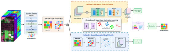
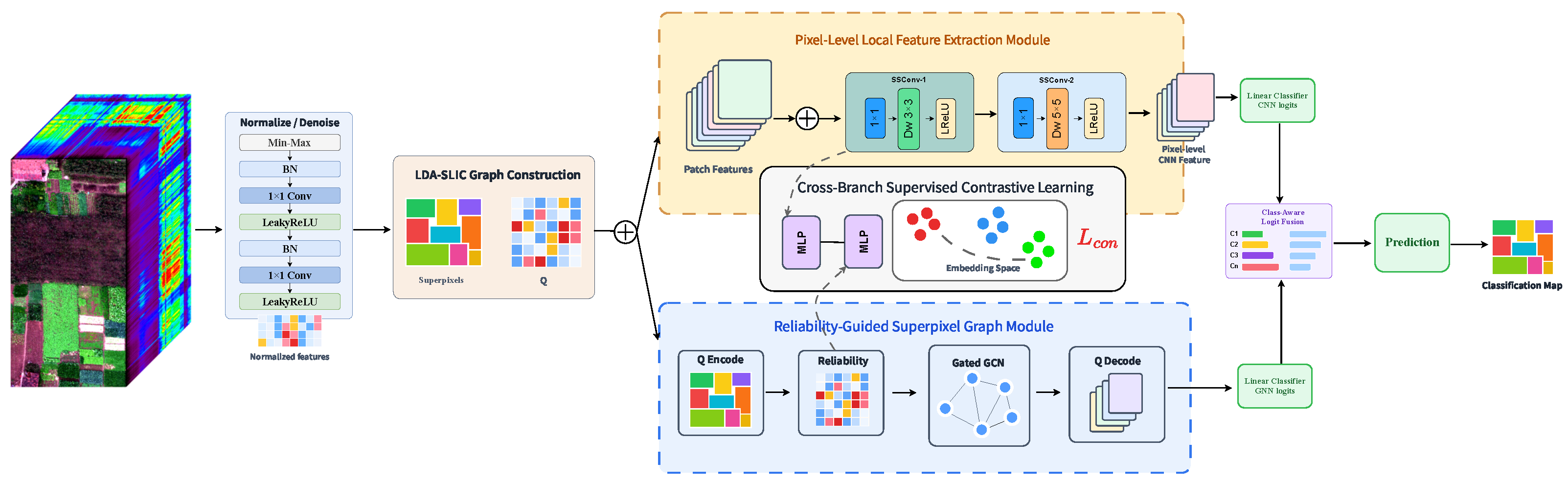
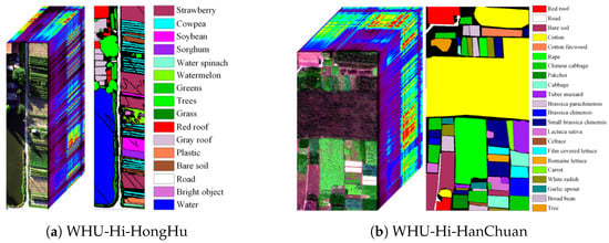
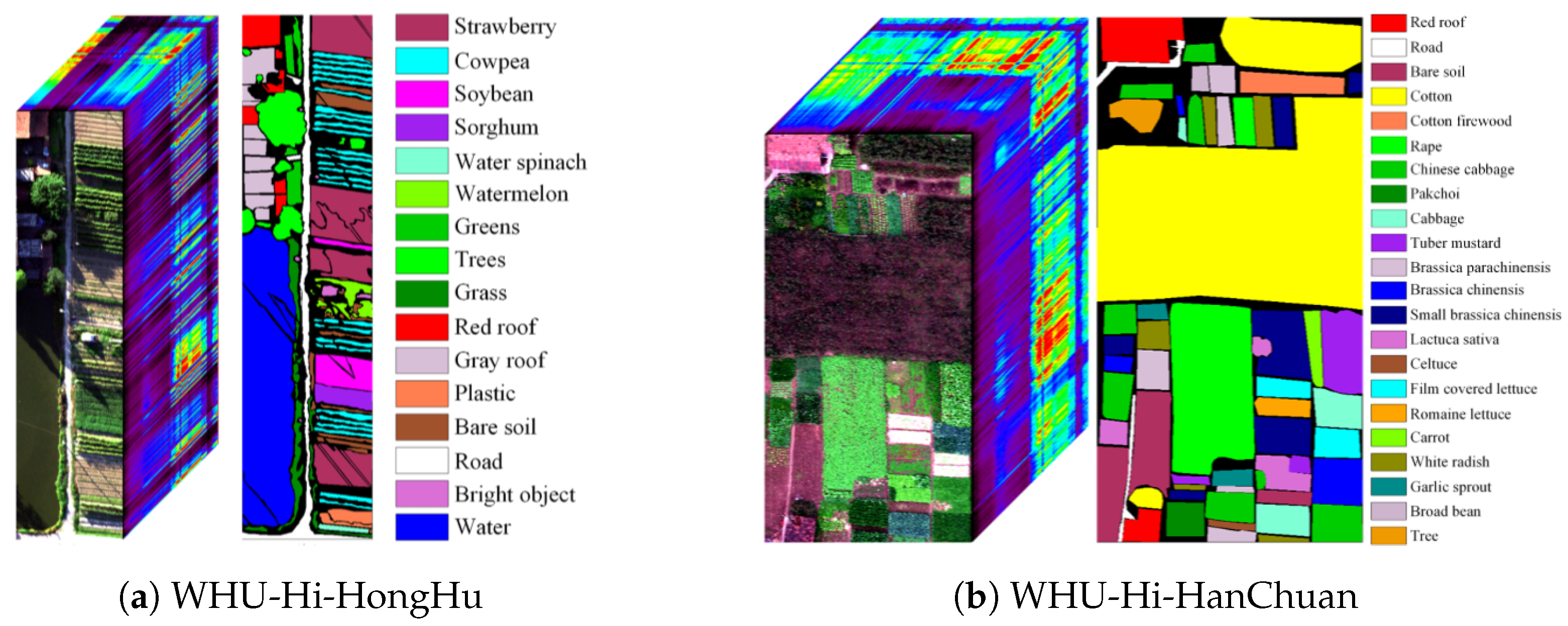
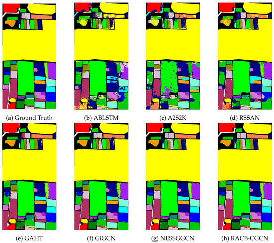
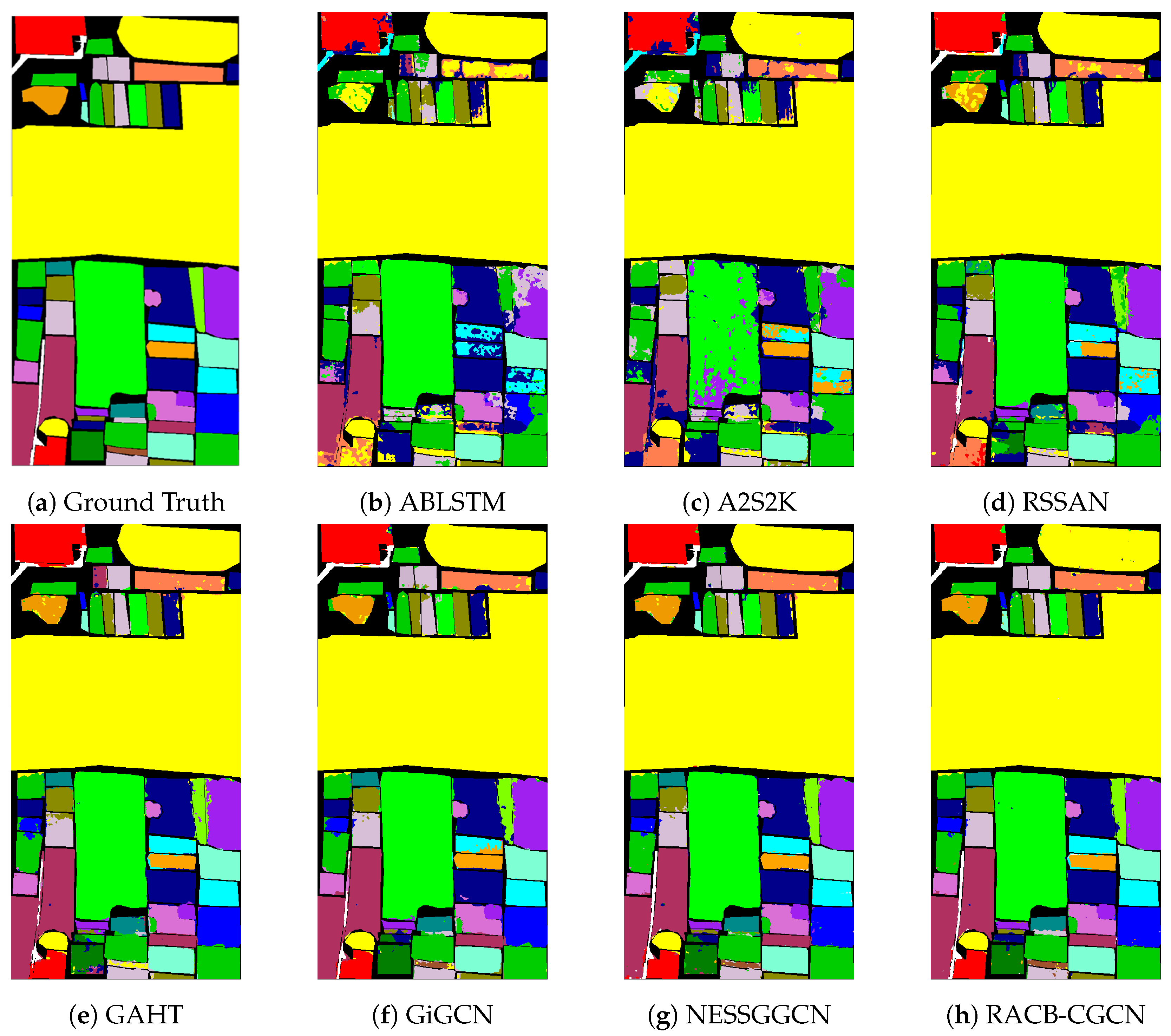
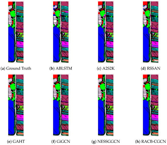
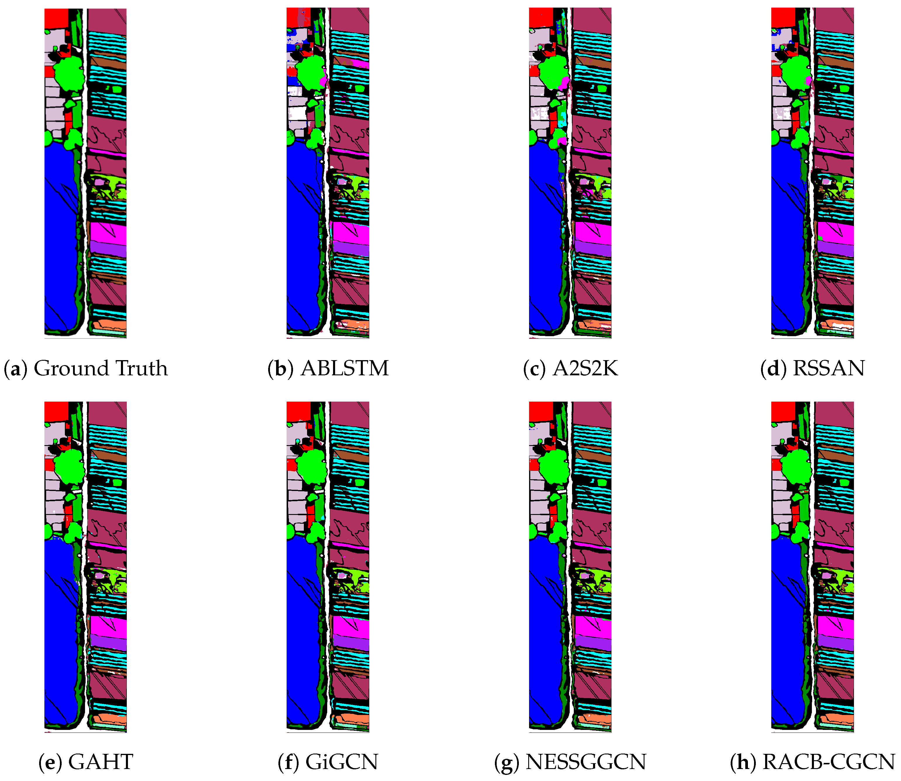
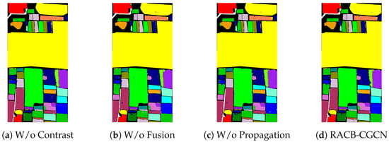
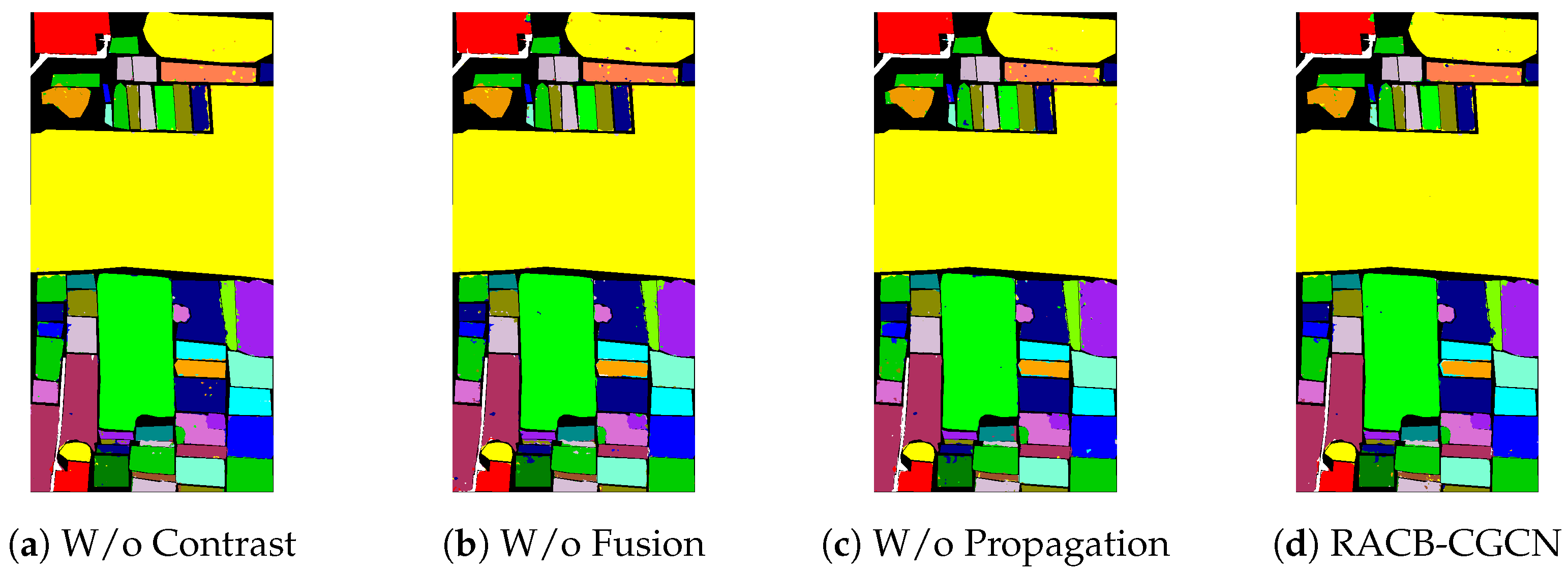
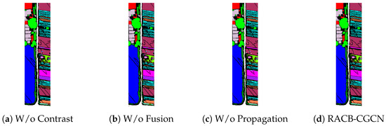
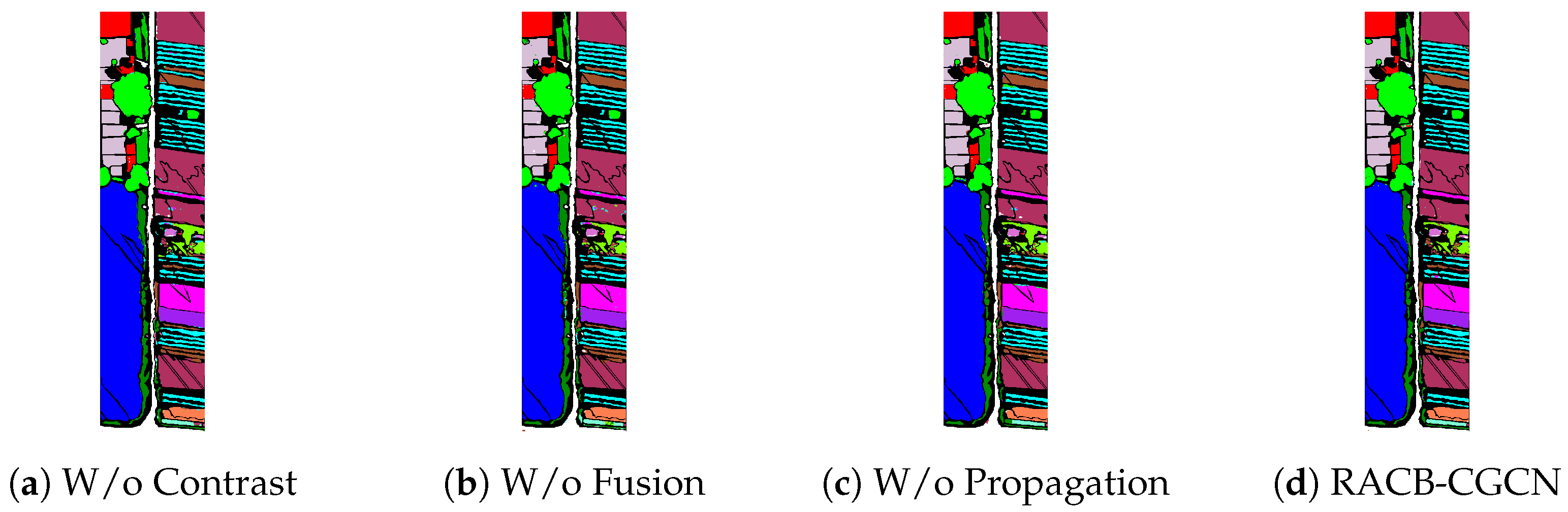
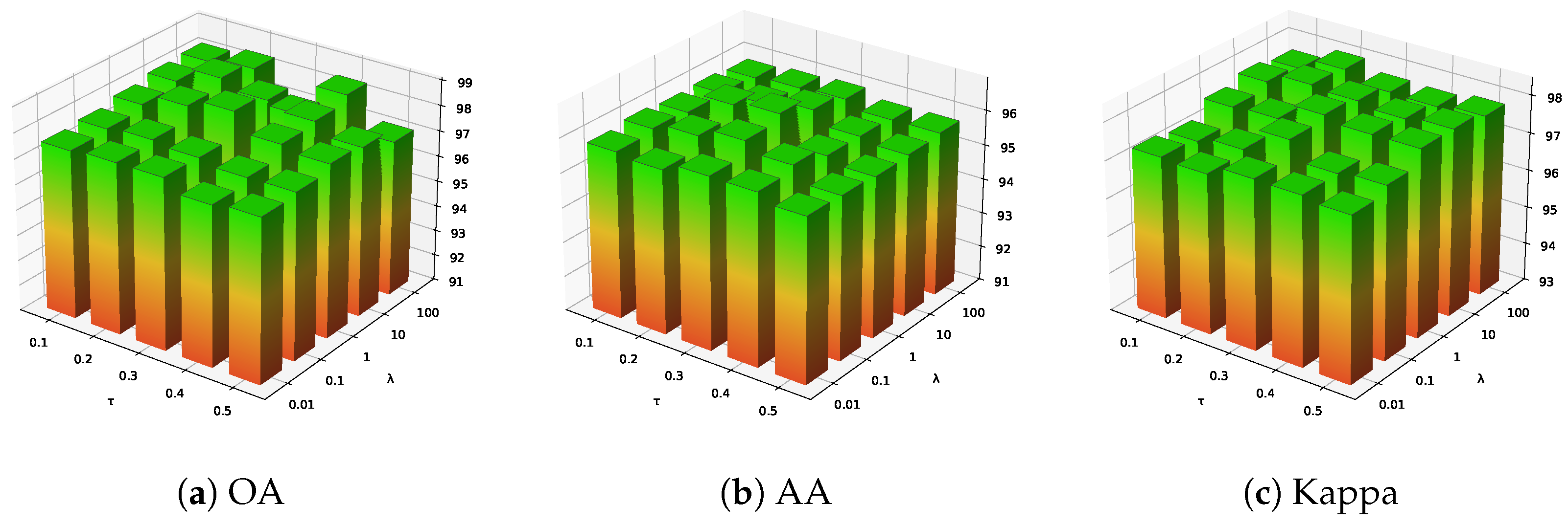
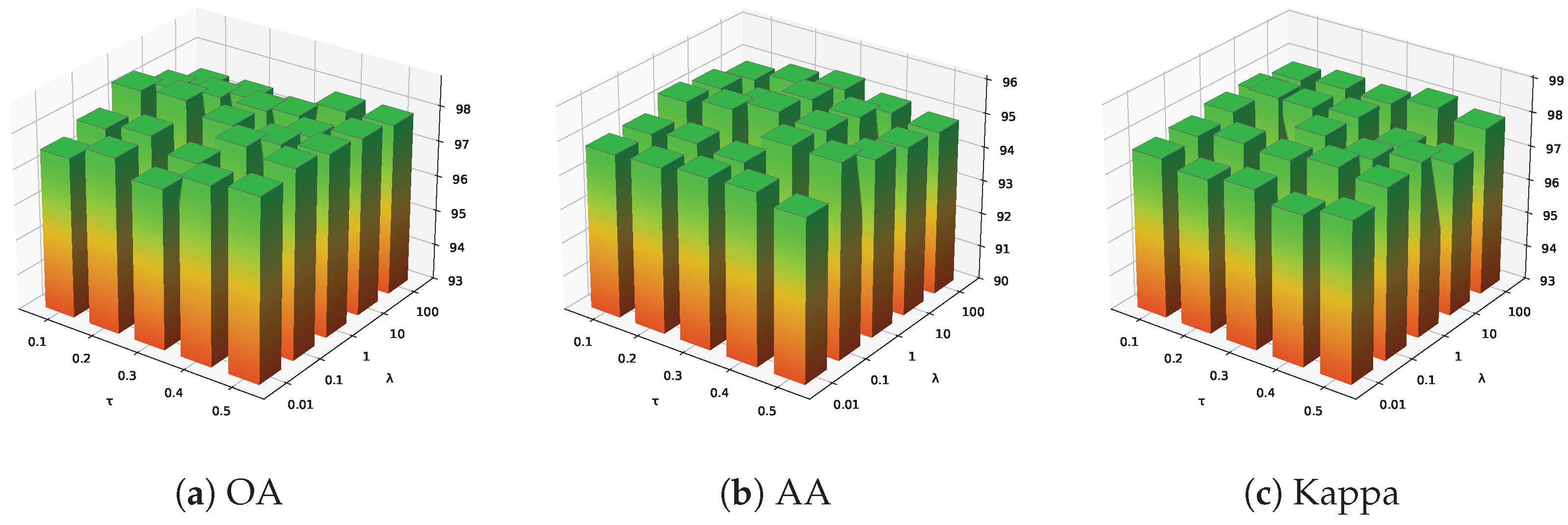
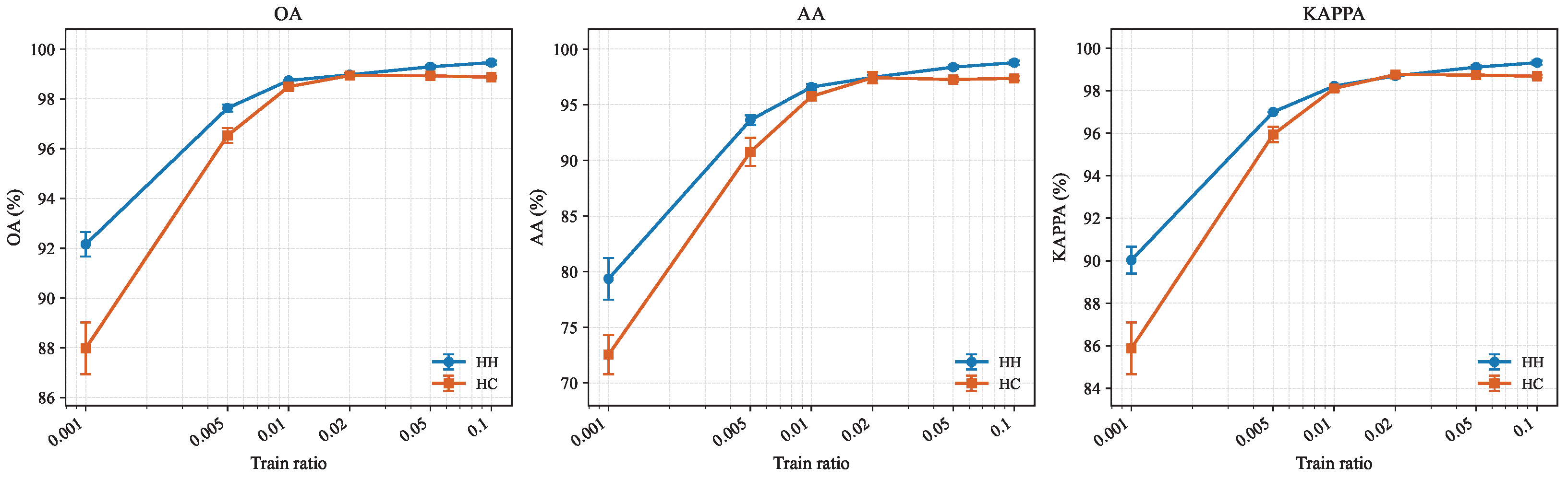

Disclaimer/Publisher’s Note: The statements, opinions and data contained in all publications are solely those of the individual author(s) and contributor(s) and not of MDPI and/or the editor(s). MDPI and/or the editor(s) disclaim responsibility for any injury to people or property resulting from any ideas, methods, instructions or products referred to in the content. |
© 2026 by the authors. Licensee MDPI, Basel, Switzerland. This article is an open access article distributed under the terms and conditions of the Creative Commons Attribution (CC BY) license.