Automatic Modulation Recognition Based on RadioAlign Feature Adaptation, Scale Attention, and a Bayesian Residual Branch

Abstract

To address amplitude scaling, phase rotation, local misalignment, and ambiguous decision boundaries under low-SNR and non-cooperative reception conditions, we propose an Attention RadioAlign Bayesian Residual Network (ABRNet) for automatic modulation recognition. ABRNet takes raw I/Q sequences as input. It first employs a RadioAlign module to estimate and apply bounded learnable transformations that aim to mitigate amplitude-phase and local-offset input variations. A scale-attention module then adaptively weights short-term phase transitions, local waveform patterns, and long-term envelope variations. Finally, a Bayesian residual branch adds a small stochastic residual to the deterministic logits and estimates the predictive mean, variance, and entropy as reliability measures. Across five random seeds, ABRNet achieves a mean overall accuracy of 63.4668% (sample standard deviation: 0.0583%), a low-SNR accuracy of 34.2864% (0.1399%), a high-SNR accuracy of 92.6473% (0.0630%), and a Macro F1 score of 65.7086% (0.0784%). The error-detection AUROC is 0.894092 (0.000370), the expected calibration error is 0.016618 (0.001703), and the Brier score is 0.434423 (0.000127). With approximately 287 K parameters, ABRNet provides classification and predictive reliability measures in an end-to-end I/Q processing pipeline.

1. Introduction

Automatic modulation recognition (AMR) is a key component of non-cooperative communications, spectrum sensing, and intelligent receivers. Its objective is to identify the modulation format of a received signal without prior knowledge of transmitter parameters. Deep learning methods can learn discriminative features directly from raw I/Q sequences and have achieved strong performance on public modulation-recognition datasets [1]. However, under low-SNR conditions and in the presence of amplitude-phase variations or local sampling offsets, class boundaries can become blurred, increasing the difficulty of classification.

Existing end-to-end models face two related challenges. First, modulation-discriminative patterns occur at different temporal scales: PSK signals depend on phase transitions, QAM signals contain joint amplitude-phase structures, and AM/FM signals are expressed mainly through envelope or frequency variations. Fixed-scale convolutions cannot simultaneously accommodate all of these characteristics. Second, deterministic networks usually output a single softmax probability vector, which does not directly provide a risk ranking for erroneous or boundary samples. Overconfident predictions in low-confidence regions may consequently mislead downstream demodulation or manual review.

To address these issues, we propose ABRNet, which organizes automatic modulation recognition into three connected stages. First, RadioAlign estimates and applies bounded learnable transformations that aim to mitigate amplitude-phase and local-offset input variations. Scale attention then selects effective waveform responses, and a deterministic residual backbone learns the primary classification boundary. Finally, a Bayesian residual branch adds a small residual to the deterministic logits without replacing the primary classification head, thereby providing predictive-risk information. The three design elements address input adaptation, discriminative temporal-scale selection, and reliability estimation, respectively. We evaluate classification performance, module effects, and predictive reliability using OA, low-/high-SNR OA, Macro F1, error-detection AUROC, ECE, Brier score, and coverage accuracy.

2. Related Work

Existing automatic modulation-recognition studies can be organized into three directions: end-to-end representation learning, multi-scale feature extraction and input adaptation, and predictive uncertainty and calibration. The following subsections review representative approaches in each direction and then clarify their relationship to ABRNet.

2.1. Deep Learning for Modulation Recognition

Traditional modulation recognition methods rely on handcrafted features, such as higher-order cumulants, cyclic spectra, and constellation representations, followed by conventional classifiers. Although these features are physically interpretable, their design and parameter selection require substantial domain expertise, and their discriminative power often degrades at low SNRs [2]. Deep learning integrates feature extraction and classification into a unified end-to-end optimization framework. Given an input I/Q sequence $X$, the network learns a mapping from the raw signal to the logits of the modulation classes:

$$l=f_{\theta }(X),$$

(1)

where $\theta$ denotes the network parameters, and $l\in {ℝ}^C$ denotes the unnormalized scores for the C modulation classes. The probability of the c-th class is then obtained using the softmax function:

$$p_c={\displaystyle \frac{\exp (l_c)}{{\displaystyle \sum _{j=1}^C\exp }(l_j)}},\hspace{1em}c=1,2,\cdots ,C.$$

(2)

Here, $l_c$ denotes the unnormalized logit for class c, $l_j$ denotes the logit for class j in the denominator, and C is the total number of modulation classes. Logits are the unnormalized scores produced by the classification head and are converted into class probabilities only after softmax. During supervised training, the predicted probabilities are aligned with the ground-truth labels using the cross-entropy loss:

$${\mathcal{L}}_{CE}=-{\displaystyle \sum _{c=1}^C{y}_c}\log p_c,$$

(3)

where $y_c$ is the c-th component of the one-hot target vector. CNN-based models are effective at extracting local waveform patterns, while recurrent architectures, such as RNNs, LSTMs, and GRUs, capture temporal dependencies. CNN–RNN hybrid models combine local feature extraction with sequential context modeling [3,4]. However, amplitude scaling, phase rotation, temporal misalignment, and strong noise can still lead to unstable decision boundaries in models trained directly on raw I/Q inputs [5].

Complex-valued and multi-channel networks further show that jointly modeling the I/Q components helps retain amplitude-phase structure. Under amplitude-phase variations, local offsets, and low-SNR conditions, however, an end-to-end backbone must still address both input variations and class discrimination.

2.2. Multi-Scale Attention and Wireless Signal Feature Adaptation

Modulated signals contain discriminative information at different temporal scales. Short-scale convolutions more readily capture phase transitions and local symbol changes, whereas longer-scale convolutions are better suited to envelope trends and frequency variations. Existing methods use multi-scale convolutions, multi-feature fusion, vision transformers, skip attention, and temporal-hybrid structures to enlarge receptive fields and emphasize informative temporal or scale-specific responses [6,7,8,9,10,11]. These approaches alleviate the inability of a single kernel size to represent both local phase structure and longer-term envelope variation.

In input-adaptation research, parameter estimation, phase transformation, and cross-domain adaptation aim to mitigate receiver-gain, carrier-phase, and local-offset variations [12,13,14]. In non-cooperative reception, such factors can broaden the input distribution of samples from the same modulation class and increase overlap between different classes. If the backbone must learn these nuisance variations implicitly, it must simultaneously perform input adaptation, feature extraction, and class discrimination.

Input adaptation and scale attention therefore have distinct but complementary functions: the former addresses amplitude, phase, and local-offset variations, whereas the latter selects more discriminative temporal scales from the transformed waveform representation.

2.3. Bayesian Uncertainty and Probability Evaluation

Beyond input adaptation and multi-scale feature extraction, automatic modulation recognition also requires an assessment of predictive reliability. Deterministic neural networks learn a fixed point estimate and produce a single probability vector, whose maximum softmax value may not faithfully reflect reliability for low-SNR samples, overlapping class boundaries, or distribution shifts. Bayesian neural networks represent parameters as distributions and obtain predictive means, variances, and entropies through repeated sampling, although training and inference are more complex [15]. Deep ensembles train multiple models and estimate risk from their predictive disagreement, but require additional training, storage, and inference cost [16]. MC dropout retains stochastic dropout during inference and approximates a predictive distribution through repeated forward passes, although its uncertainty estimate depends on dropout settings [15,16]. Probability-calibration methods such as temperature scaling primarily adjust the correspondence between confidence and empirical accuracy at low cost, but do not by themselves provide a complete sampled uncertainty distribution [17].

For modulation recognition, low-SNR and easily confused classes are more likely to produce high-risk predictions. Reliability evaluation should therefore consider not only OA, but also whether uncertainty ranks erroneous samples effectively and whether confidence agrees with empirical accuracy. Error-detection AUROC, ECE, Brier score, and coverage-accuracy evaluate error-risk ranking, probability calibration, and selective recognition, respectively.

Directly replacing the complete classification head with Bayesian layers can produce a sampled distribution, but sampling perturbations and prior regularization may affect the primary classification boundary. To retain a deterministic classification path while providing risk information in a lightweight I/Q pipeline, ABRNet models Bayesian estimation as a residual branch that makes only a small modification to deterministic logits. The deterministic path performs primary class discrimination, while repeated residual sampling provides the predictive mean, variance, entropy, and probability-evaluation information. These research routes, representative methods, and their implications for ABRNet are summarized in Table 1.

Table 1. Comparison of related methods and implications for ABRNet.

Research Route	Representative Methods	Input/Features	Advantage	Limitation	Implication for ABRNet
Handcrafted features	Cumulants, cyclic spectra, constellations	Statistical or time-frequency features	Physical interpretability	Low-SNR degradation; manual design	Retain signal-structure information
End-to-end networks	CNN, CLDNN, ResNet, complex networks	Raw I/Q	Joint feature and classifier learning	No explicit adaptation to input variations	Use a light-weight I/Q backbone
Multi-scale/attention	Feature fusion, ViT, skip attention	Multi-receptive-field features	Select local and long-term responses	Often assume aligned inputs	Select scales after input adaptation
Input adaptation	Parameter estimation, phase transformation, transfer	Transformed I/Q	Mitigate input variations	May introduce transformation instability	Constrain transformation parameters
Uncertainty methods	Confidence modeling, Bayesian models, ensembles	Predictive distributions	Risk information and probability evaluation	Extra inference cost	Use a small residual branch

In summary, existing studies generally improve automatic modulation recognition from a single perspective, such as input adaptation, multi-scale feature extraction, or predictive reliability. ABRNet assigns RadioAlign, scale attention, and the Bayesian residual branch to input adaptation, discriminative feature selection, and risk-information expression, respectively.

3. Methods

3.1. Overall Architecture

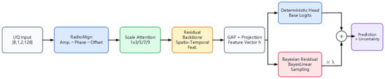
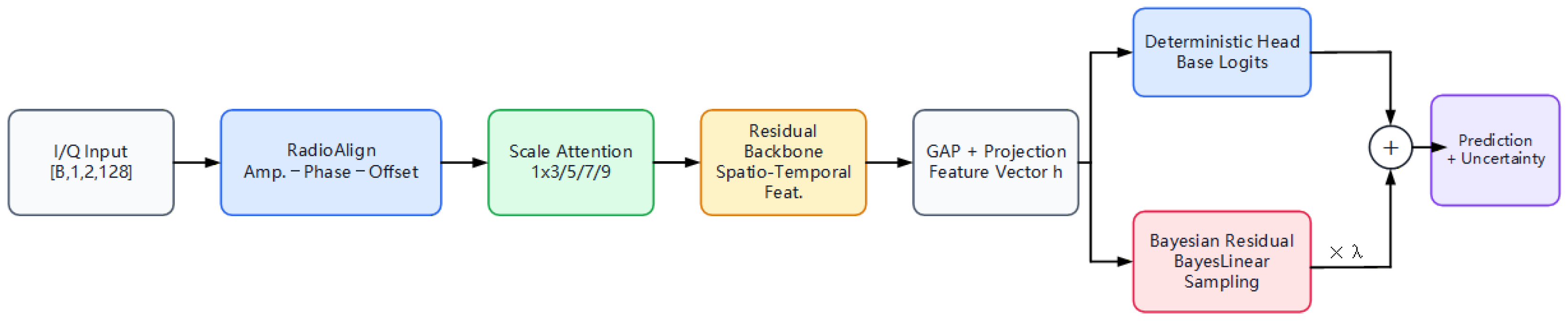
Figure 1 illustrates the overall architecture of ABRNet. Raw I/Q sequences first pass through RadioAlign, which estimates bounded amplitude, phase, and local-offset transformations. Scale attention then selects temporal receptive-field responses for the transformed representation. The residual backbone and I/Q fusion layer produce a global feature vector; a deterministic head produces base logits, and the Bayesian residual branch produces a small stochastic residual. Their sum produces the final logits, while repeated Bayesian sampling provides reliability measures.

Figure 1. Overall architecture of ABRNet.

3.2. RadioAlign Input Adaptation Module

In non-cooperative reception scenarios, received I/Q sequences may exhibit amplitude scaling, phase rotation, and local sampling offsets. If these variations enter the classification backbone directly, the model must learn input adaptation and class boundaries simultaneously, which can reduce feature-utilization efficiency. RadioAlign therefore estimates and applies sample-level bounded learnable transformations that aim to mitigate these input variations before feature extraction.

Let the raw input be

$$X=\left[\begin{array}{c}I\\ Q\end{array}\right]\in {ℝ}^{2\times L},$$

(4)

where the $I$ and $Q$ components denote the in-phase and quadrature sequences of length L, respectively. The RadioAlign branch extracts a sample-level context vector using a lightweight one-dimensional convolution followed by global pooling. A parameter estimator then predicts three alignment parameters. To prevent excessive modification of the input waveform, each parameter is constrained to a predefined range using a bounded activation function.

$$\theta ={\theta }_{\max }\tanh (o_{\theta }),\hspace{1em}s=\exp \left(s_{\max }\tanh (o_s)\right),\hspace{1em}\Delta ={\Delta }_{\max }\tanh (o_{\Delta }),$$

(5)

where $o_{\theta }$, $o_s$, and $o_{\Delta }$ are the outputs of the parameter estimator, while ${\theta }_{\max }$, $s_{\max }$, and ${\Delta }_{\max }$ control the maximum magnitudes of phase rotation, logarithmic amplitude scaling, and local translation, respectively. ${\theta }_{\max }$ bounds the phase-rotation angle, ${\Delta }_{\max }$ bounds the magnitude of the local translation, and $s_{\max }$ bounds the logarithmic amplitude-scale term inside the exponential. Thus, the amplitude factor remains positive and satisfies exp(−$s_{\max }$) ≤ s ≤ exp($s_{\max }$). These fixed bounds constrain transformation strength rather than applying a logarithm directly to I/Q amplitudes. RadioAlign then applies a differentiable transformation to the input using the estimated amplitude factor $\mathrm{s}$, phase-rotation angle $\theta$, and local-offset parameter $\Delta$:

$$\tilde{X}={\mathcal{T}}_{\Delta }\left(s\left[\begin{array}{cc}\cos \theta & -\sin \theta \\ \sin \theta & \cos \theta \end{array}\right]X\right).$$

(6)

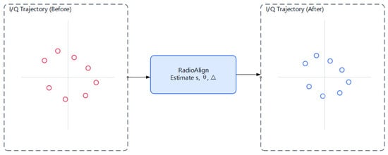
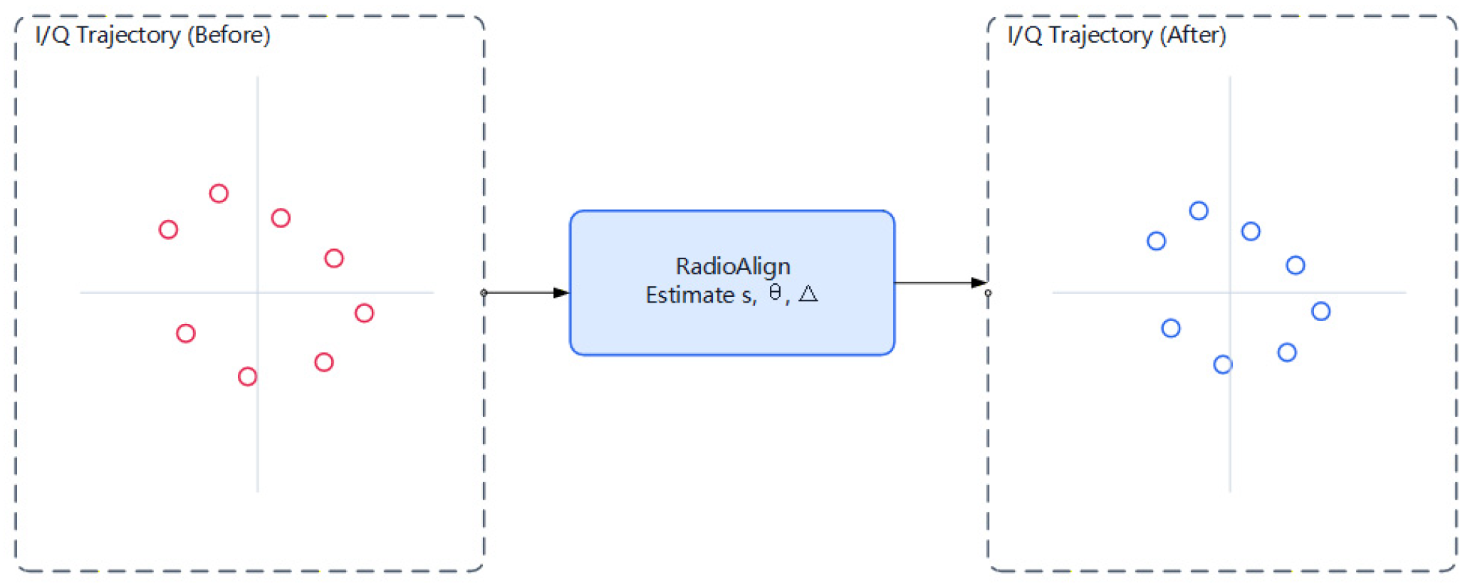
where $\tilde{X}$ denotes the aligned I/Q sequence, and ${\mathcal{T}}_{\Delta }(\cdot )$ denotes the local resampling or translation operation controlled by the estimated offset. The rotation matrix, amplitude factor, and local resampling respectively act on I/Q-plane rotation, amplitude scaling, and temporal-position variation. The module does not require ground-truth channel parameters at inference time; instead, all adaptation parameters are estimated directly from the input sample. The overall RadioAlign transformation is illustrated in Figure 2.

Figure 2. Schematic diagram of the RadioAlign module. Red circles represent the I/Q trajectory before RadioAlign, whereas blue circles represent the I/Q trajectory after alignment.

3.3. Scale Attention Feature Extraction Module

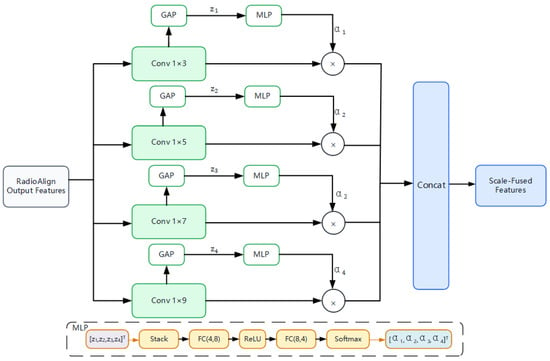
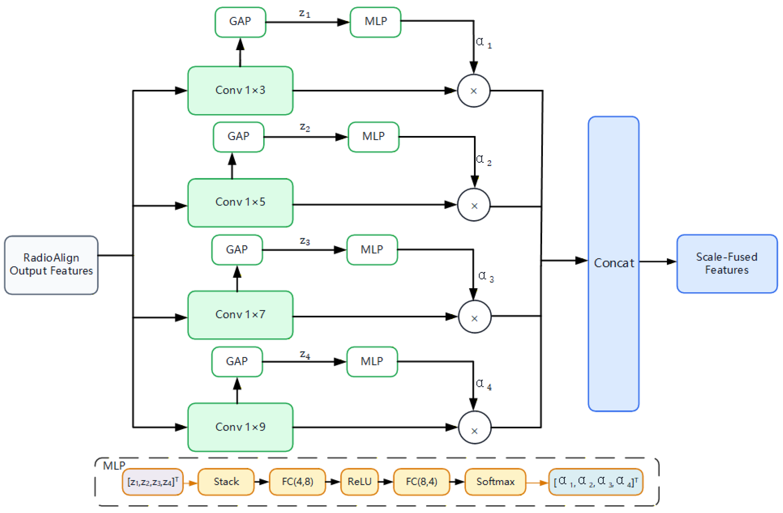
The aligned representation still contains discriminative patterns at multiple temporal scales. To select the most informative temporal scales for each sample, a multi-scale attention module is applied after RadioAlign. Let the convolutional kernel of the m-th branch be $W_m$. The corresponding scale-specific feature is computed as follows:

$$F_m=\sigma \left(W_m*\tilde{X}+b_m\right),\hspace{1em}m=1,2,\dots ,M,$$

(7)

where * denotes convolution, $b_m$ is the bias of the m-th branch, $\sigma (\cdot )$ is the nonlinear activation function, and M is the number of scale branches. Rather than assigning equal weights to all branches, the model derives sample-specific attention weights from their global responses. Global average pooling is first applied to each branch:

The four branches use temporal kernels of 1 × 3, 1 × 5, 1 × 7, and 1 × 9. With feature length preserved, smaller kernels emphasize short-term structures such as phase transitions and symbol neighborhoods, whereas larger kernels represent longer envelope and frequency trends. Adjacent kernel sizes increase by two to control scale spacing, branch count, and parameter count. This is an empirical configuration for an input length of 128 and is not presented as an optimum obtained from systematic sensitivity analysis.

$$z_m=\mathrm{GAP}(F_m),\hspace{1em}u={[z_1,z_2,\cdots ,z_M]}^T.$$

(8)

The pooled scale statistics $u$ are then concatenated and passed through a lightweight two-layer MLP. A softmax function converts the resulting gating scores into normalized scale weights:

$$e=g(u)=W_2\delta (W_{1}u+b_1)+b_2,$$

(9)

$$a_m={\displaystyle \frac{\exp (e_m)}{{\displaystyle \sum _{r=1}^M\exp }(e_r)}},\hspace{1em}m=1,2,\cdots ,M,$$

(10)

where $\mathrm{GAP}(\cdot )$ denotes global average pooling, $\delta (\cdot )$ is the ReLU activation function, $g(\cdot )$ denotes the two-layer weight-generation network, and $a_m$ is the normalized attention weight assigned to the m-th scale. To preserve the channel structure of each branch, the weighted scale features are concatenated:

$$F_{SA}=\mathrm{Concat}\left(a_1{F}_1,a_2{F}_2,\cdots ,a_M{F}_M\right),$$

(11)

where $F_{SA}$ denotes the scale-attention-fused feature map. RadioAlign and multi-scale attention perform complementary functions. RadioAlign first applies bounded learnable transformations that aim to mitigate input variations caused by amplitude scaling, phase rotation, and temporal misalignment. Multi-scale attention then weights short-, medium-, and long-range waveform patterns according to the characteristics of each aligned sample. Short- and medium-scale responses help characterize the phase and amplitude structures of PSK and QAM signals, whereas longer-scale responses are useful for capturing the envelope and frequency variations of AM and FM signals. This cascade performs input adaptation before scale-specific feature extraction, allowing the backbone to focus more directly on modulation discrimination [8]. The architecture of the multi-scale attention module is illustrated in Figure 3.

Figure 3. Architecture of the multi-scale attention module.

3.4. Bayesian Residual Branch

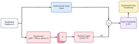
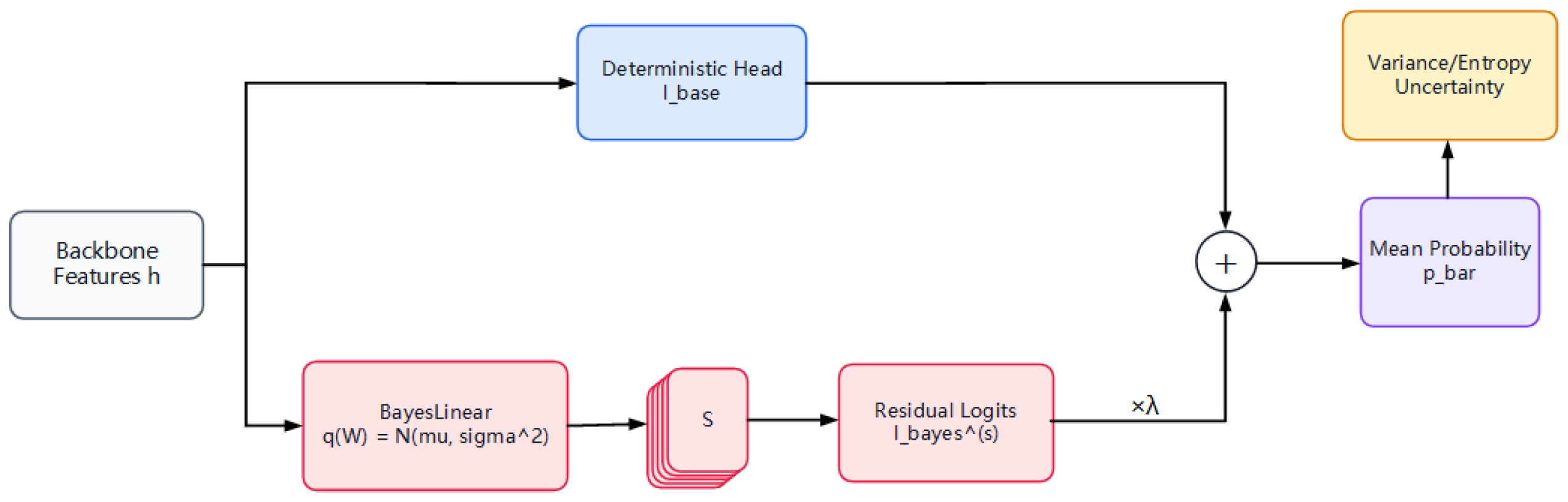
After RadioAlign-based feature adaptation and multi-scale attention, the residual backbone extracts high-level representations. Let the global feature vector produced by the backbone be $h$. The deterministic classification head then produces the base logits as follows:

$$l_{base}=W_{c}h+b_c.$$

(12)

where $W_c$ and $b_c$ are the parameters of the deterministic classification head, and $l_{base}$ denotes the base logits. The deterministic head defines the primary decision boundary and is not directly affected by Bayesian weight sampling. It therefore provides a stable classification path on which the residual branch can operate.

The Bayesian residual branch takes the same global feature vector $h$ as input. Rather than being represented by deterministic point estimates, the weights and biases of the Bayesian linear layer are modeled using a variational posterior:

$$W_b~q_{\varphi }(W_b),\hspace{1em}{b}_b~q_{\varphi }(b_b).$$

(13)

where $W_b$ and $b_b$ denote the weight and bias of the Bayesian residual layer, respectively, and $q_{\varphi }(\cdot )$ is the variational posterior governed by the parameters $\varphi$. The residual logits obtained from the s-th Monte Carlo draw are expressed as follows:

$$\Delta l^{(s)}=W_b^{(s)}h+b_b^{(s)}.$$

(14)

where $\Delta l^{(s)}$ denotes the Bayesian residual logits obtained from the s-th draw. The final logits are computed as follows:

$$l^{(s)}=l_{base}+\lambda \Delta l^{(s)}.$$

(15)

where $\lambda$ is the residual scaling coefficient that controls the influence of the Bayesian residual on the deterministic decision boundary. In this design, the Bayesian layer provides only a scaled residual contribution rather than replacing the deterministic classifier. This preserves the primary classification path while enabling Monte Carlo estimation of the predictive distribution. The mean predictive probability and predictive variance over multiple draws are computed as follows:

$$\overline{p}={\displaystyle \frac{1}{S}}{\displaystyle \sum _{s=1}^S\mathrm{softmax}}(l^{(s)}),$$

(16)

$$\mathrm{Var}(p)={\displaystyle \frac{1}{S}}{\displaystyle {\displaystyle \sum _{s=1}^S}{\left(\mathrm{softmax}(l^{(s)})-\overline{p}\right)}^2}.$$

(17)

where S denotes the number of Monte Carlo draws, $\overline{p}$ is the mean predictive probability, and $\mathrm{Var}(p)$ is the predictive variance. The dispersion of predictive probabilities across repeated samples is used to characterize model uncertainty. The Bayesian residual branch and its interaction with the deterministic classification head are illustrated in Figure 4.

Figure 4. Schematic diagram of the Bayesian residual branch.

3.5. Loss Function and Inference

The ABRNet training objective consists of a classification term and a KL regularization term. For the logits $l^{(s)}$ obtained from the s-th Monte Carlo draw, the cross-entropy loss is ${\mathcal{L}}_{CE}^{(s)}$. The classification losses are then averaged across draws:

$${\mathcal{L}}_{cls}={\displaystyle \frac{1}{S_t}}{\displaystyle \sum _{s=1}^{S_t}{\mathcal{L}}_{CE}^{(s)}},$$

(18)

where $S_t$ denotes the number of Monte Carlo samples drawn per input during training. The Bayesian residual branch is additionally regularized using the KL divergence between the variational posterior and the prior distribution:

$${\mathcal{L}}_{KL}=D_{KL}\left(q_{\varphi }(W_b,b_b)\Vert p(W_b,b_b)\right),$$

(19)

where $p(W_b,b_b)$ denotes the prior distribution over the parameters of the Bayesian residual layer. The final training objective is expressed as follows:

$$\mathcal{L}={\mathcal{L}}_{cls}+\beta {\mathcal{L}}_{KL},$$

(20)

where $\beta$ is the coefficient controlling the strength of KL regularization. During inference, the Bayesian residual branch is sampled multiple times, and the averaged predictive probabilities are used for classification. The predicted class is selected as the class with the highest averaged probability:

$$\widehat{y}=\arg {\max }_c{\overline{p}}_c,$$

(21)

Here, $\overline{p}$ denotes the averaged predictive probability vector, ${\overline{p}}_c$ denotes its component corresponding to class $c$, and $\widehat{y}$ denotes the final predicted class. This rule is used to compute OA, confusion matrices, and other classification metrics. In parallel, the probabilities obtained by applying softmax to each sampled logit vector are averaged to compute predictive variance, predictive entropy, confidence, ECE, and Brier score.

Specifically, during training, each input sample passes through RadioAlign, scale attention, and the deterministic residual backbone to obtain the base logits. The Bayesian residual branch is then sampled $S_t$ times; the cross-entropy losses from these samples are averaged and combined with the KL regularization term to form the total loss. Gradients are back-propagated from the total loss, the learnable parameters are updated using Adam, and the best model weights are selected according to validation performance. During inference, the residual branch is sampled $S$ times, and the averaged predictive probabilities are used to determine the final class. The sampled probabilities are further summarized to compute predictive variance, predictive entropy, and calibration metrics. The sampling counts, learning rate, KL weight, warmup schedule, and other implementation settings are given in Section 4.1.

4. Experimental Validation and Performance Analysis

4.1. Dataset and Experimental Setup

All experiments are conducted on RadioML2016.10a, a GNU radio-generated dataset containing 11 analog and digital modulation classes. Each class contains samples at 20 SNR levels ranging from −20 to 18 dB in 2 dB increments. Each sample consists of two I/Q channels with a sequence length of 128. To preserve the class and SNR distributions, samples within each modulation–SNR combination are divided into training, validation, and test sets at a ratio of 6:2:2. The resulting dataset configuration is summarized in Table 2.

Table 2. Dataset parameters and data split.

Item	Setting
Dataset	RadioML2016.10a
Number of classes	11
Modulation types	8PSK, AM-DSB, AM-SSB, BPSK, CPFSK, GFSK, PAM4, QAM16, QAM64, QPSK, WBFM
SNR range	−20 dB to 18 dB, step 2 dB
Samples per (mod, snr)	1000
Sample shape	2 × 128 I/Q
Total samples	220,000
Train/Val/Test split	132,000/44,000/44,000

The validation set is used for model selection and the test set only for final evaluation. Models are trained with Adam and a fixed-step learning-rate schedule. The Bayesian residual layer uses a mixture-of-Gaussians prior, $\lambda$ = 0.20, a KL weight of 0.0005, and KL warmup. $\lambda$ was selected in a single exploratory validation analysis and then fixed as an empirical setting after considering difficult-class performance and probability calibration; the test set was not used for this choice. Three samples are used during training and ten during inference. The reported conclusions reflect classification and reliability under the unified RadioML2016.10a simulation setting. Key parameters are listed in Table 3.

Table 3. Key training parameters.

Item	Setting
Optimizer	Adam
LR schedule	Fixed step
Initial learning rate	0.001
Weight decay	1 × 10−4
Bayesian prior	Mixture of Gaussians
Residual scale	0.20
KL weight	5 × 10−4
KL warmup	30 epochs
Monte Carlo samples (training/inference)	3/10

4.2. Evaluation Metrics

We evaluate classification performance and reliability. OA is the overall test-set accuracy; low-SNR and high-SNR OA are computed below 0 dB and at or above 0 dB; and Macro F1 weights all classes equally. Error-detection AUROC evaluates whether uncertainty separates incorrect from correct samples, ECE evaluates confidence calibration, and Brier score evaluates the squared error of probabilistic outputs. Coverage is the fraction of samples retained after risk ranking, and retained-sample accuracy is recomputed on that subset.

4.3. Background Comparison with Classical Model Results

ABRNet is compared with literature-reported results on RadioML2016.10a for contextual reference. ResNet, CLDNN, MCLDNN, PET-CGDNN, and CV-ResNet represent residual convolutional, convolutional-recurrent, parameter-estimation, and complex-valued directions. Because data splits, training schedules, and implementations differ across studies, this comparison provides background rather than a strict ranking under a unified protocol. The background comparison is summarized in Table 4.

Table 4. Background comparison of ABRNet and literature-reported results.

Model	Type	Params	OA/%
ResNet	Residual CNN	3098 K	42.51
CLDNN	CNN + LSTM	76 K	59.14
MCLDNN	Multi-ch. CNN + LSTM	405 K	60.51
PET-CGDNN	Param. Est. + CNN/GRU/DNN	71 K	60.60
CV-ResNet	Complex-valued ResNet	364 K	46.27
ABRNet (ours)	Attn + RadioAlign + BayesRes	287 K	63.4668 ± 0.0583 (five runs)

ABRNet is reported as the mean plus sample standard deviation across five runs; the table is provided to place the result in its research context.

4.4. SNR and Modulation Class Analysis

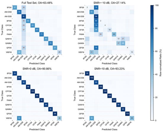
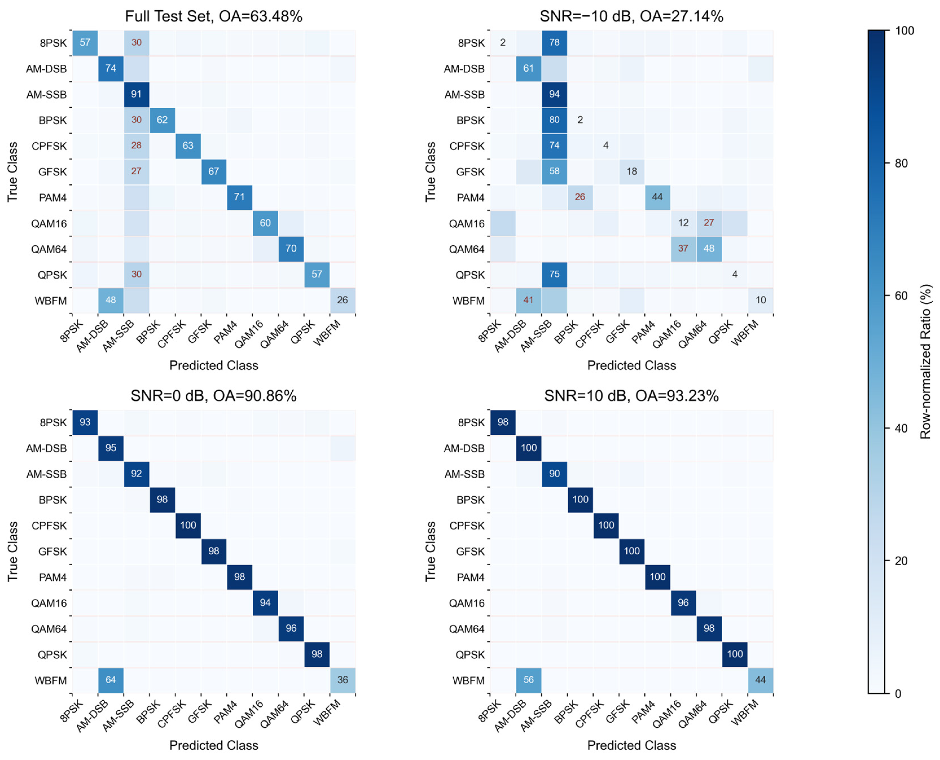
Across five runs, ABRNet obtains a low-SNR OA of 34.2864 ± 0.1399% and a high-SNR OA of 92.6473 ± 0.0630%. Class accuracies, confusion patterns, and Figure 5 and Figure 6 are from a single representative run and are used to analyze error modes rather than multi-run average performance. Between −20 and −12 dB, modulation-discriminative patterns are severely masked by noise; as SNR increases, phase, amplitude, and envelope patterns become clearer. The bounded learnable transformations in RadioAlign aim to mitigate input variations but cannot restore modulation information lost in noise-dominated observations.

Figure 5. Confusion matrices under representative SNR conditions.

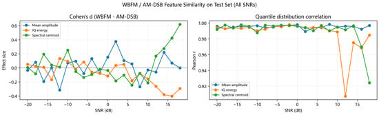
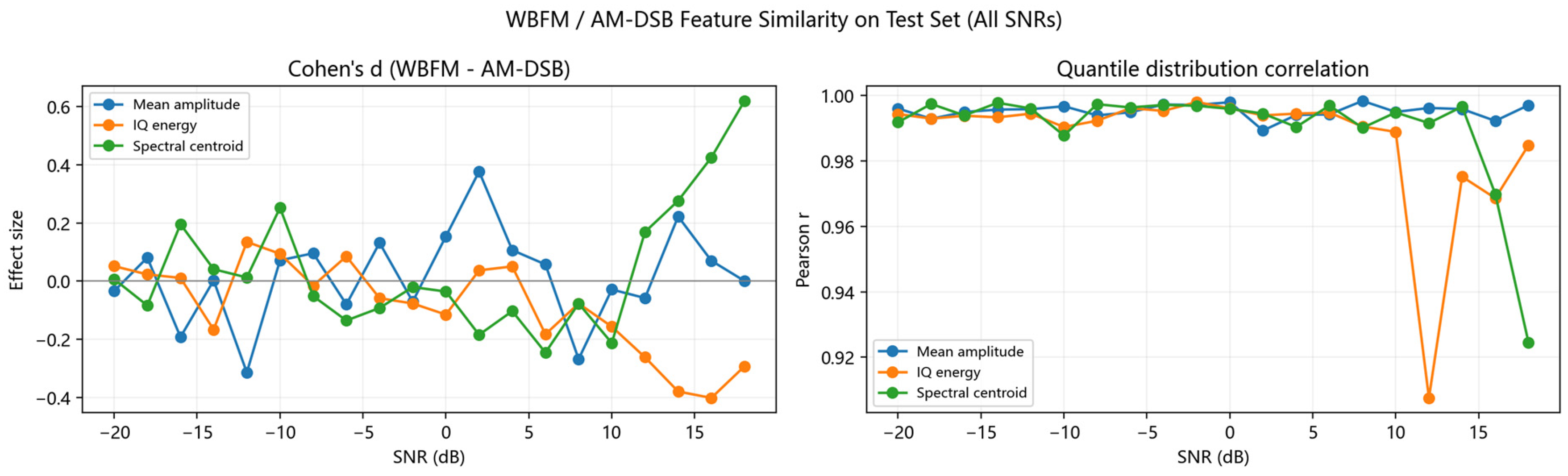
Figure 6. Feature similarity statistics for WBFM and AM-DSB test samples.

In the representative run, ABRNet performs well on AM-SSB, AM-DSB, PAM4, and QAM64, while WBFM remains difficult. The WBFM, QAM16, QAM64, and mean QAM accuracies are 26.05%, 59.38%, 70.53%, and 64.95%, respectively. Major confusion patterns include WBFM classified as AM-DSB and several PSK/FSK classes classified as AM-SSB. The recorded WBFM-to-AM-DSB confusion count in this representative run is 1937.

The observed confusion patterns have signal-level explanations. At low SNR or when modulation features are weak, WBFM and AM-DSB may exhibit similarly concentrated I/Q noise clouds because noise masks envelope and instantaneous-frequency differences. For QPSK, 8PSK, and BPSK, noise spreads phase states and broadens the constellation structure. CPFSK and GFSK depend on continuous phase or frequency variation and can be confused with broadly distributed classes such as AM-SSB when short-term frequency changes are obscured. QAM16 and QAM64 both combine amplitude and phase variation; at low SNR, constellation levels are compressed and amplitude-ring boundaries become blurred, producing substantial intra-QAM confusion.

To analyze the asymmetric WBFM/AM-DSB confusion, the representative test run compares the two classes by SNR using amplitude mean, I/Q energy, and spectral centroid. The two classes are closer in amplitude and energy at low SNR, while spectral-centroid differences become more visible at higher SNR. WBFM is classified as AM-DSB substantially more often than the reverse error, indicating that WBFM samples are more likely to fall within the AM-DSB decision region under the current data and model. This evidence supports an interpretation of the observed asymmetric confusion without asserting complete equivalence or a unique causal mechanism.

4.5. Module Ablation and Complexity Analysis

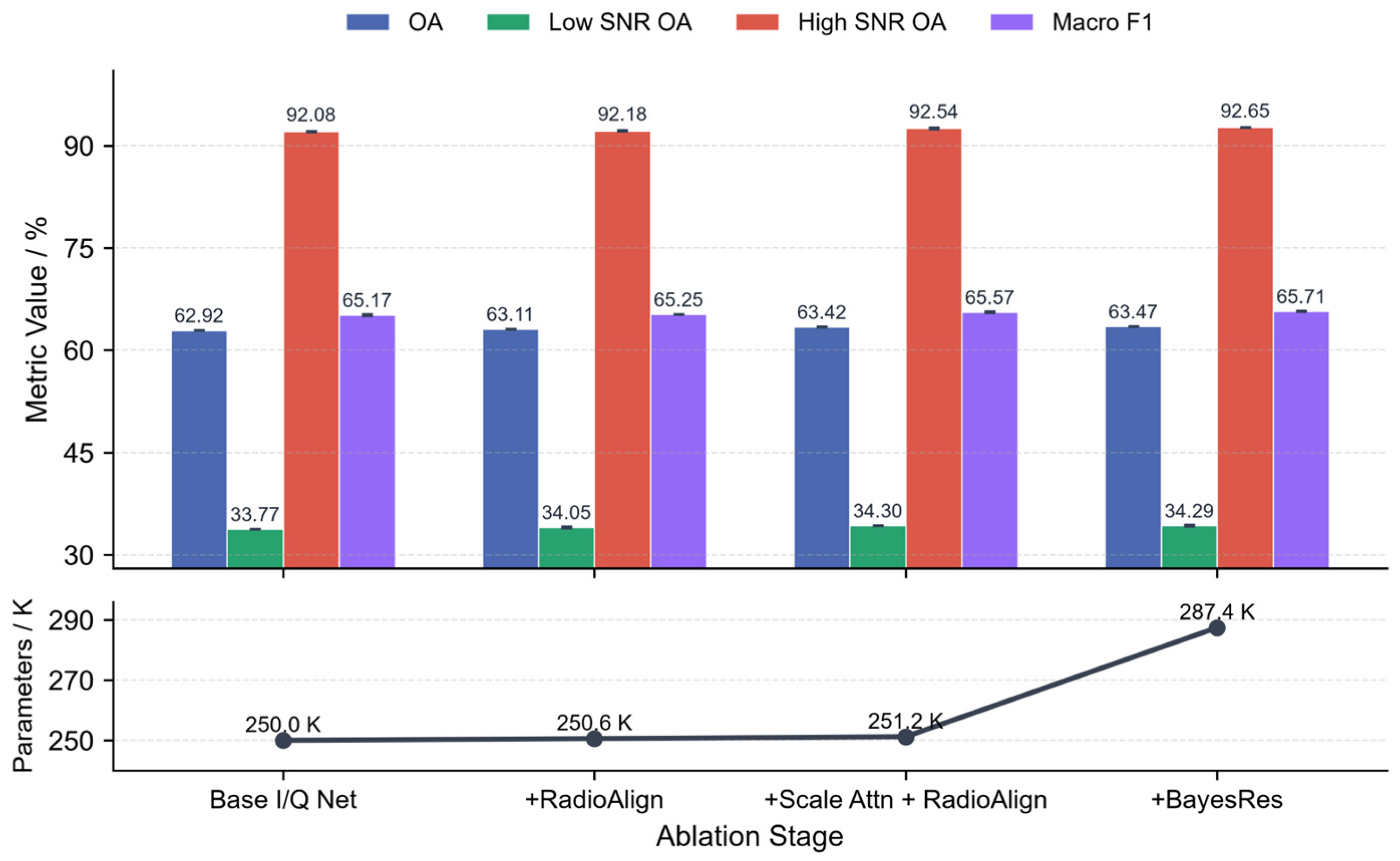
A four-stage ablation compares the base I/Q network, + RadioAlign, + Scale Attention + RadioAlign, and + Bayesian Residual Branch (full ABRNet). All stages use the same data split and training protocol. Figure 7 and Table 5 report the mean and sample standard deviation across five runs.

Figure 7. Module ablation results for ABRNet.

Table 5. Module ablation results of ABRNet.

Architecture	OA/% (Mean ± SD)	OA 95% CI/%	Low-SNR OA/% (Mean ± SD)	High-SNR OA/% (Mean ± SD)	Macro F1/% (Mean ± SD)	Parameters
Base I/Q network	62.9245 ± 0.0427	62.8715–62.9775	33.7655 ± 0.0648	92.0836 ± 0.0945	65.1665 ± 0.1415	249,995
+RadioAlign	63.1141 ± 0.0571	63.0432–63.1849	34.0500 ± 0.1289	92.1782 ± 0.0734	65.2461 ± 0.0644	250,574
+Scale Attention + RadioAlign	63.4168 ± 0.0726	63.3267–63.5069	34.2955 ± 0.0714	92.5382 ± 0.1570	65.5709 ± 0.1386	251,182
+Bayesian Residual Branch (full ABRNet)	63.4668 ± 0.0583	63.3944–63.5392	34.2864 ± 0.1399	92.6473 ± 0.0630	65.7086 ± 0.0784	287,428

Table 5 reports the mean and sample standard deviation over five random seeds (2026, 891, 2685, 7620, and 8387). The OA 95% confidence intervals use a two-sided t interval ($n$ = 5, $df$ = 4).

Relative to the base I/Q network, adding RadioAlign yields an OA mean increase of 0.1895 percentage points (95% CI: 0.1151–0.2640; p = 0.002112) and a low-SNR OA mean increase of 0.2845 percentage points (p = 0.026057). This input-adaptation stage provides a stable mean classification gain across the five runs.

Relative to the base I/Q network, the Scale Attention + RadioAlign stage yields an OA mean increase of 0.4923 percentage points (95% CI: 0.3658–0.6187; p = 0.000415). Its low/high-SNR OA and Macro F1 mean increases are 0.5300, 0.4545, and 0.4044 percentage points, with p values of 0.000353, 0.003743, and 0.016747. With the Bayesian residual branch, full ABRNet achieves an OA mean increase of 0.5423 percentage points (95% CI: 0.4361–0.6485; p = 0.000144) and a macro F1 mean increase of 0.5421 percentage points (p = 0.001518).

Full ABRNet has 287,428 parameters (approximately 287 K) and a weight-file size of approximately 1.15 MB, an increase of about 14.97% relative to the base I/Q network. The additional parameters mainly arise from the Bayesian residual classification head. Inference computation increases with input length and the number of Bayesian samples.

4.6. Bayesian Residual Effectiveness and Calibration Analysis

The Bayesian residual branch is evaluated through classification-boundary preservation, error-risk ranking, probability calibration, and selective recognition. It adds a small stochastic residual after the deterministic logits rather than replacing the deterministic classification head. The correct/error grouping, point estimates of AUROC, ECE, and Brier score, and coverage-accuracy curves in this section are based on a single representative run; multi-run summaries are reported in the abstract, Table 4 and Table 5, and the conclusion.

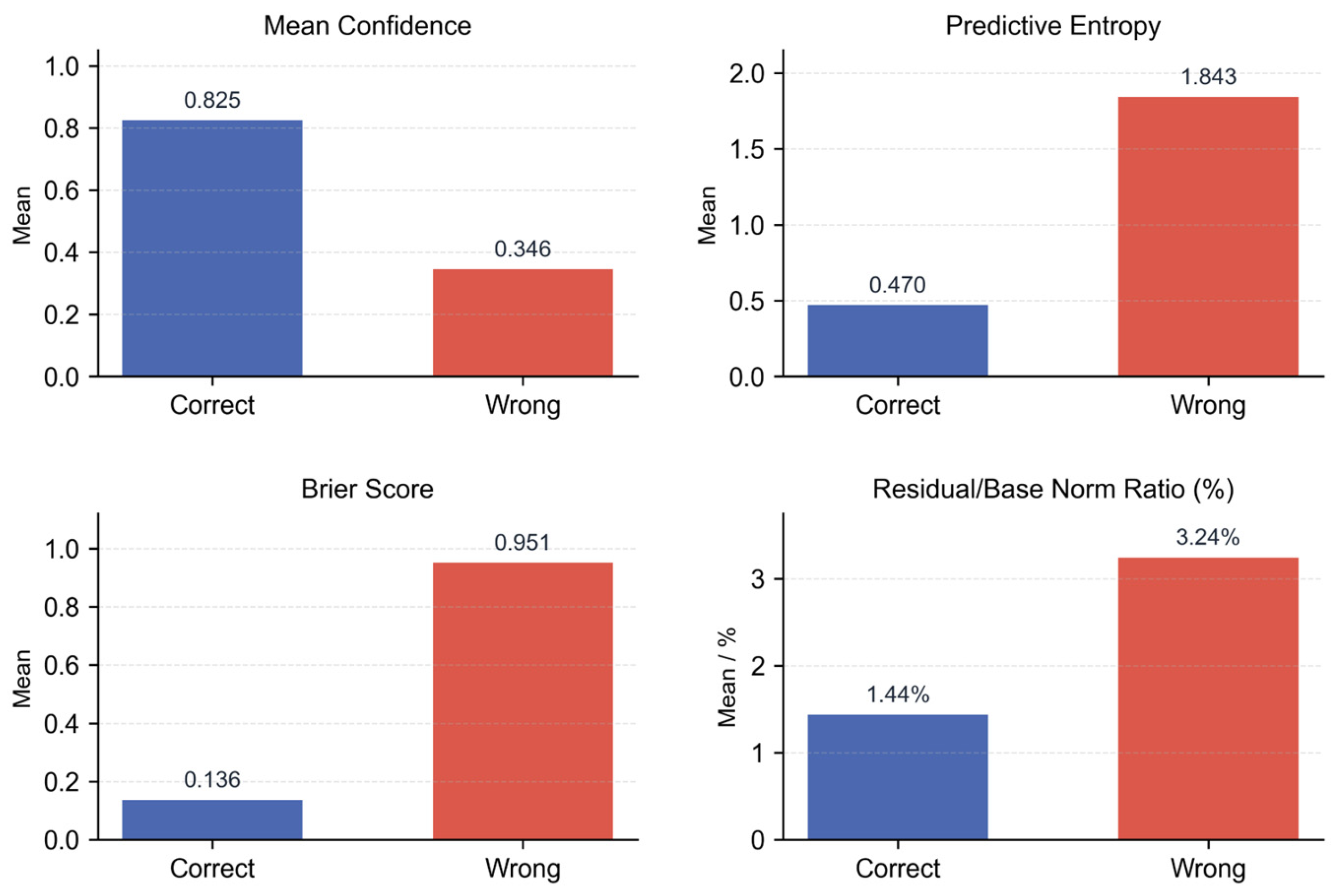
After adding the Bayesian residual branch, mean OA changes from 63.4168% to 63.4668% and mean high-SNR OA changes from 92.5382% to 92.6473%. In the representative run, the residual perturbation is small, while incorrect samples have a higher relative residual, suggesting that it may provide risk-related information. The corresponding effects of the Bayesian residual classification head are visualized in Figure 8.

Figure 8. Visualization of the effectiveness of the Bayesian residual classification head.

For error-risk ranking and probability calibration, repeated sampling produces predictive mean, variance, and entropy. In the representative run, error-detection AUROC is 0.8937. Mean confidence is 0.8247 for correct samples and 0.3455 for incorrect samples; predictive entropy is 0.4702 and 1.8435; and Brier score is 0.1364 and 0.9510, respectively. Overall ECE is 0.0159 and the Brier score is 0.4338.

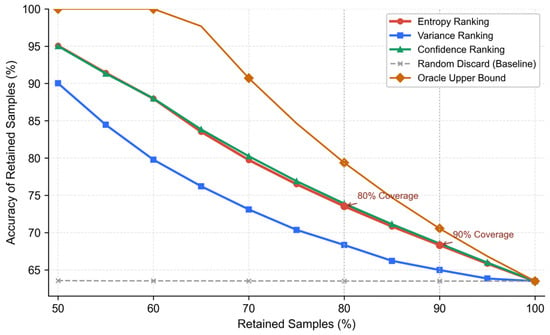
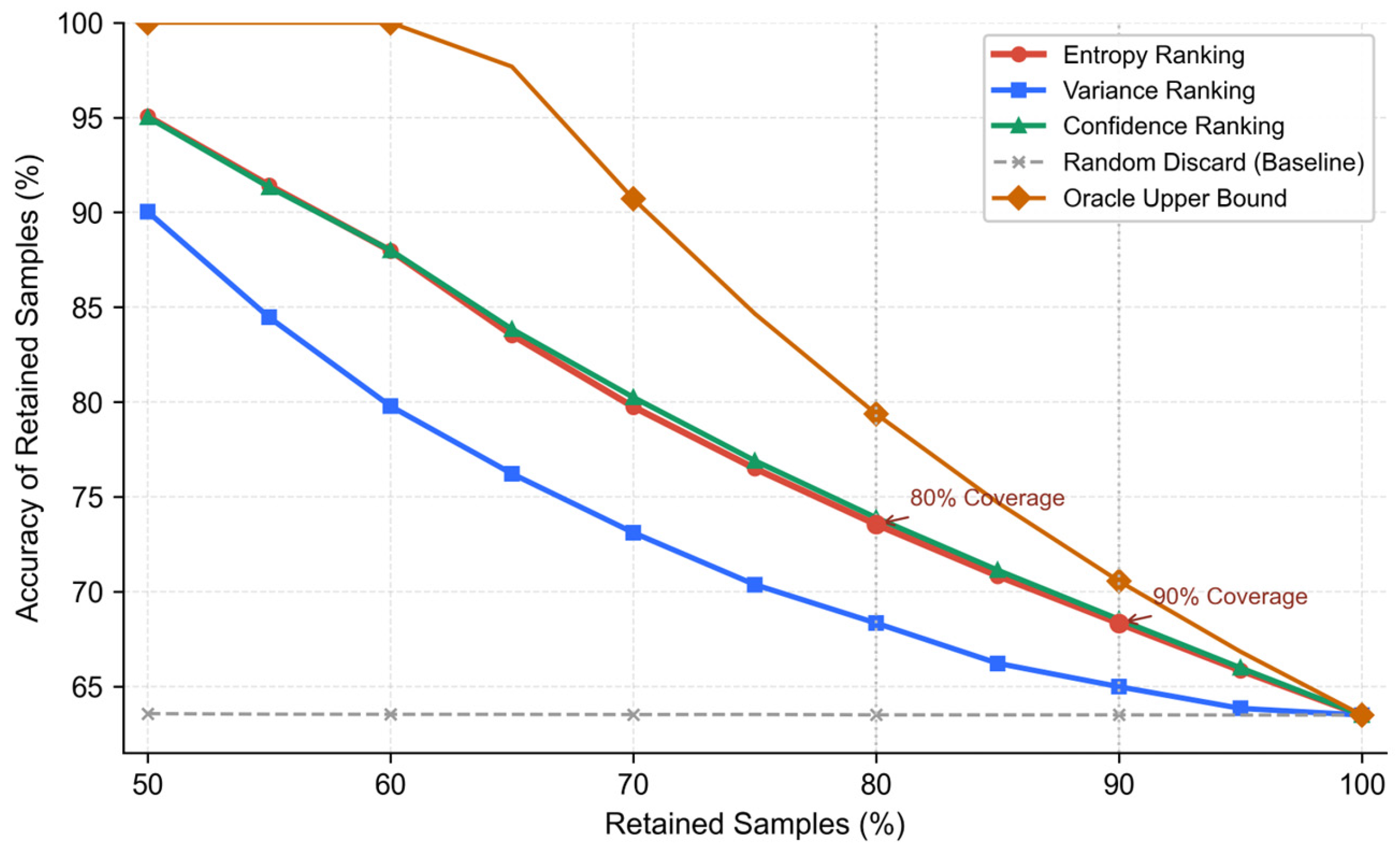
For selective prediction, coverage is the retained fraction of samples after risk ranking and retained-sample accuracy is recomputed on that subset. Ranking by predictive entropy from low to high and retaining the lowest-entropy 50% of samples gives 95.06% accuracy. At 50% and 80% coverage, random discard yields 63.57% and 63.50%, approximately the full-test-set OA, whereas predictive-entropy ranking yields 95.06% and 73.55%. Thus, entropy ranking preferentially retains more reliable samples. The oracle curve represents ideal risk ranking, and the entropy curve lies between the random baseline and oracle reference.

This ranking can provide a risk-ranking reference for subsequent rejection or manual review strategies.

Predictive-entropy and confidence coverage-accuracy curves nearly overlap, with a maximum difference below one percentage point between 50% and 100% coverage. Predictive-variance ranking yields a retained-sample accuracy of 90.03% at 50% coverage. As coverage increases, the ranking threshold is relaxed and more uncertain samples are retained, so retained-sample accuracy decreases; the curve shape is also influenced by the SNR and class-difficulty distribution of the test set. The resulting coverage–accuracy curves are shown in Figure 9.

Figure 9. Coverage–accuracy curves.

5. Conclusions

This paper presents ABRNet, an automatic modulation-recognition network that combines RadioAlign feature adaptation, scale attention, and a Bayesian residual branch. The method performs I/Q input adaptation, multi-scale feature selection, and Bayesian residual refinement of deterministic logits.

Across five random seeds, ABRNet achieves an OA of 63.4668 ± 0.0583%, a low-SNR OA of 34.2864 ± 0.1399%, a high-SNR OA of 92.6473 ± 0.0630%, and a Macro F1 of 65.7086 ± 0.0784%, with approximately 287 K parameters. Error-detection AUROC, ECE, and Brier score are 0.894092 ± 0.000370, 0.016618 ± 0.001703, and 0.434423 ± 0.000127, respectively.

The ablation results show that RadioAlign, scale attention, and the Bayesian residual branch jointly improve classification metrics; full ABRNet has an OA mean increase of 0.5423 percentage points relative to the base I/Q network. Reliability analysis from a single representative run shows that predictive-entropy ranking can preferentially retain more reliable samples and can provide a risk-ranking reference for later rejection or manual review. Future work will analyze confusable classes such as WBFM and AM-DSB and validate the method on cross-dataset and real-signal scenarios.

References

- O’Shea, T.J.; Roy, T.; Clancy, T.C. Over-the-Air Deep Learning Based Radio Signal Classification. IEEE J. Sel. Top. Signal Process. 2018, 12, 168–179. [Google Scholar] [CrossRef] [Scilit]
- Dobre, O.A.; Abdi, A.; Bar-Ness, Y.; Su, W. Survey of Automatic Modulation Classification Techniques: Classical Approaches and New Trends. IET Commun. 2007, 1, 137–156. [Google Scholar] [CrossRef] [Scilit]
- Xu, J.; Luo, C.; Parr, G.; Luo, Y. A Spatiotemporal Multi-Channel Learning Framework for Automatic Modulation Recognition. IEEE Wirel. Commun. Lett. 2020, 9, 1629–1632. [Google Scholar] [CrossRef] [Scilit]
- Wang, Y.; Gui, G.; Ohtsuki, T.; Adachi, F. Multi-Task Learning for Generalized Automatic Modulation Classification Under Non-Gaussian Noise With Varying SNR Conditions. IEEE Trans. Wirel. Commun. 2021, 20, 3587–3596. [Google Scholar] [CrossRef] [Scilit]
- Xu, Z.; Hou, S.; Fang, S.; Hu, H.; Ma, Z. A Novel Complex-Valued Hybrid Neural Network for Automatic Modulation Classification. Electronics 2023, 12, 4380. [Google Scholar] [CrossRef] [Scilit]
- Wang, Z.; Zhang, W.; Zhao, Z.; Tang, P.; Zhang, Z. Robust Automatic Modulation Classification via a Lightweight Temporal Hybrid Neural Network. Sensors 2024, 24, 7908. [Google Scholar] [CrossRef] [Scilit] [PubMed]
- Wu, T.; Zheng, W.; Liu, L. Automatic Modulation Recognition Using Vision Transformers with Cross-Layer Feature Fusion and Kolmogorov–Arnold Representation. Wirel. Netw. 2025, 31, 3981–3992. [Google Scholar] [CrossRef] [Scilit]
- Shang, P.; Guo, L.; Zou, D.; Wang, X.; Gao, S.; Liu, P. A novel multi-feature extraction based automatic modulation classification. J. Syst. Eng. Electron. 2025, 36, 1407–1427. [Google Scholar] [CrossRef] [Scilit]
- Han, H.; Ren, Z.; Li, L.; Zhu, Z. Automatic Modulation Classification Based on Deep Feature Fusion for High Noise Level and Large Dynamic Input. Sensors 2021, 21, 2117. [Google Scholar] [CrossRef] [Scilit] [PubMed]
- Zhang, W.; Xue, K.; Yao, A.; Sun, Y. CTRNet: An Automatic Modulation Recognition Based on Transformer-CNN Neural Network. Electronics 2024, 13, 3408. [Google Scholar] [CrossRef] [Scilit]
- Zheng, G.; Zang, B.; Yang, P.; Zhang, W.; Li, B. FE-SKViT: A Feature-Enhanced ViT Model with Skip Attention for Automatic Modulation Recognition. Remote Sens. 2024, 16, 4204. [Google Scholar] [CrossRef] [Scilit]
- Zhang, F.; Luo, C.; Xu, J.; Luo, Y. An Efficient Deep Learning Model for Automatic Modulation Recognition Based on Parameter Estimation and Transformation. IEEE Commun. Lett. 2021, 25, 3287–3290. [Google Scholar] [CrossRef] [Scilit]
- Chen, H.; Guo, W.; Kang, K.; Hu, G. Automatic Modulation Recognition Method Based on Phase Transformation and Deep Residual Shrinkage Network. Electronics 2024, 13, 2141. [Google Scholar] [CrossRef] [Scilit]
- Deng, W.; Xu, Q.; Li, S.; Wang, X.; Huang, Z. Cross-Domain Automatic Modulation Classification Using Multimodal Information and Transfer Learning. Remote Sens. 2023, 15, 3886. [Google Scholar] [CrossRef] [Scilit]
- Abdar, M.; Pourpanah, F. A Review of Uncertainty Quantification in Deep Learning: Techniques, Applications and Challenges. Inf. Fusion 2021, 76, 243–297. [Google Scholar] [CrossRef] [Scilit]
- Gawlikowski, J.; Tassi, C.R.N. A Survey of Uncertainty in Deep Neural Networks. Artif. Intell. Rev. 2023, 56, 1513–1589. [Google Scholar] [CrossRef] [Scilit]
- Xia, G.; Bouganis, C.-S. Augmenting the Softmax with Additional Confidence Scores for Improved Selective Classification with Out-of-Distribution Data. Int. J. Comput. Vis. 2024, 132, 3714–3752. [Google Scholar] [CrossRef] [Scilit]
Disclaimer/Publisher’s Note: The statements, opinions and data contained in all publications are solely those of the individual author(s) and contributor(s) and not of MDPI and/or the editor(s). MDPI and/or the editor(s) disclaim responsibility for any injury to people or property resulting from any ideas, methods, instructions or products referred to in the content. |
© 2026 by the authors. Licensee MDPI, Basel, Switzerland. This article is an open access article distributed under the terms and conditions of the Creative Commons Attribution (CC BY) license.