


Abstract
Multi-criteria decision-making methods conventionally rank alternatives by aggregating normalized criterion values into a composite score, an approach that depends on the normalization scheme, requires externally determined criterion weights, and evaluates performance in absolute terms without accounting for inter-criteria dependencies. This paper proposes machine learning-based Peer-Prediction Trees for multi-criteria decision-making, a novel method that ranks alternatives by their excess performance over data-driven peer expectations. For each criterion, a leave-one-out cross-validated decision tree predicts each alternative’s value from its performance on all other criteria; the residual between observed and predicted values extracts how much the alternative outperforms the empirical trade-off structure constraining its peers. Residuals are standardized, aligned with the preferred criterion direction, and aggregated into an Excess Performance Index using uniqueness-based weights derived endogenously from the cross-validated predictive fit. The method is validated on three real-world datasets: a numeric vehicle selection problem (22 alternatives, five criteria), a fully linguistic financial performance evaluation of Turkish listed firms (32 alternatives, four criteria), and a mixed numeric-linguistic exchange-traded fund selection problem (12 alternatives, nine criteria). The contributions of this work are fourfold: (1) the introduction of peer prediction via leave-one-out cross-validated decision trees as a multi-criteria decision-making ranking paradigm that evaluates excess performance rather than absolute scores; (2) a uniqueness-based criterion weighting scheme embedded into the method, eliminating the need for separate weighting procedures; (3) native handling of numeric, linguistic, and mixed decision matrices within a single unified framework; and (4) empirical validation across three heterogeneous real-world applications demonstrating the method’s versatility and interpretability.
1. Introduction
Multi-Criteria Decision-Making (MCDM) is a branch of operations research concerned with evaluating and ranking a finite set of alternatives characterized by multiple, often conflicting criteria [1]. Since the formalization of the field through foundational works such as the technique for order of preference by similarity to ideal solution (TOPSIS) [2], simple additive weighting (SAW) method [3], and the analytic hierarchy process (AHP) [4], MCDM has become a standard analytical framework in domains ranging from engineering design and supply chain management to environmental policy and financial portfolio selection [5]. The fundamental challenge in every MCDM problem is the same: how to aggregate heterogeneous criterion values into a single ranking that faithfully reflects the decision maker’s preferences while accounting for the structure of the data.
Despite decades of methodological development, the prevailing MCDM paradigm rests on a pipeline that has remained largely unchanged. The raw decision matrix is first normalized to render the criteria commensurable, criterion weights are then determined either subjectively or through a separate objective weighting method, and finally, a scoring or distance-based aggregation rule produces the composite ranking [6]. Each stage of this pipeline introduces modeling choices that can materially affect the result. The choice of normalization scheme (e.g., sum, vector, linear max, min–max, or others) is known to alter the final ranking even when all other parameters are held constant [7]. The weight determination step presents its own dilemma: subjective methods such as AHP require pairwise comparison judgments that are cognitively demanding and potentially inconsistent [8], while objective methods such as the entropy method [9,10] or criteria importance through inter-criteria correlation (CRITIC) [11,12] are external to the ranking procedure itself and may capture different aspects of criterion importance than the decision maker intends. These accumulated degrees of freedom mean that two analysts applying nominally the same MCDM method to the same decision matrix can arrive at different rankings simply by making different preprocessing choices. A further limitation is that virtually all established methods evaluate alternatives on the basis of their absolute or normalized performance values, implicitly counting correlated strength multiple times when criteria are interdependent. Finally, the handling of linguistic and mixed data typically requires appending fuzzy extensions that introduce additional subjective choices.
This work proposes a fundamentally different approach, a machine learning (ML)-based Peer-Prediction Tree (PPT), for MCDM problems. The PPT method replaces absolute performance evaluation with a residual-based assessment that measures how much each alternative exceeds data-driven peer expectations. For each criterion, a leave-one-out cross-validated (LOOCV) decision tree predicts the held-out alternative’s value from its performance on all other criteria. The signed residual between the observed and predicted values captures the extent to which the alternative outperforms (or underperforms) the inter-criteria trade-off structure that constrains its peers. These residuals are standardized for comparability, aligned with the preferred criterion direction, and aggregated into a composite score called the excess performance index (EPI) using uniqueness-based weights derived endogenously from the cross-validated predictive fit. The method requires only the raw decision matrix and a direction vector as inputs, with no normalization, no external weighting method (though decision-makers may use their own weights if preferred), and no additional fuzzy extension for linguistic data.
The main contributions of this work are fourfold: (1) the introduction of the PPT method via LOOCV decision trees as a novel paradigm for MCDM ranking, in which alternatives are evaluated by their excess performance over data-driven expectations rather than by absolute or normalized scores; (2) the development of a uniqueness-based criterion weighting scheme that is derived endogenously from the peer-prediction models and assigns higher weight to criteria carrying genuinely independent information, eliminating the need for separate subjective or objective weighting procedures; (3) the native handling of numeric, fuzzy linguistic, and mixed decision matrices within a single unified framework, without requiring fuzzy extensions for specialized preprocessing; and (4) the empirical validation of the method across three real-world application datasets spanning a purely numeric vehicle selection problem, a fully linguistic financial performance evaluation, and a mixed-type exchange traded fund (ETF) selection problem.
The remainder of this paper is organized as follows. Section 2 reviews the relevant literature on MCDM methods, criterion weighting, and ML applications in decision analysis. Section 3 presents the complete PPT methodology, from its conceptual foundation to all the detailed equations. Section 4 applies the PPT method to three decision matrices, compares the rankings with classical MCDM methods, and conducts a weight sensitivity analysis. Section 5 discusses the advantages, limitations, and open research questions arising from this work. Section 6 concludes with a summary of the main findings and their implications.
2. Literature Review
The literature reviewed in this section was identified through a systematic search of the Scopus, Web of Science, and Google Scholar databases using the search terms “multi-criteria decision-making”, “MCDM”, “MCDM normalization”, “criterion weighting methods”, and “machine learning MCDM”. The review focuses on foundational and highly cited works that established the main methodological streams, supplemented by recent contributions (2019 onward) that represent the current state of the art. The selection criteria prioritize methodological relevance to the three core issues addressed by our proposed method: normalization dependence, external weighting requirements, and the handling of linguistic data.
The development of formal MCDM methods began with the SAW model, in which each alternative’s composite score is formed as a weighted sum of normalized criterion values [3]. Despite its simplicity, SAW remains one of the most widely applied MCDM techniques and serves as the conceptual basis for many later extensions. The AHP, introduced by [4], contributed a structured framework for deriving criterion weights from pairwise comparisons, though the ranking step itself still reduces to weighted aggregation, as in SAW. A significant conceptual advance came with TOPSIS [2], which ranks alternatives by their simultaneous proximity to a positive ideal solution and distance from a negative ideal solution in normalized, weighted criterion space. TOPSIS introduced a geometric perspective that has since influenced numerous derivative methods; for example, MABAC (multi-attributive border approximation area comparison) determines the distance of alternatives from a calculated border approximation area [13]; MARCOS (measurement of alternatives and ranking according to compromise solution) ranks alternatives based on utility functions derived from their relationships to predefined ideal and anti-ideal reference points [14]; PROBID (preference ranking on the basis of ideal-average distance) calculates the Euclidean distance of alternatives to a series of theoretical average and ideal solutions across different performance levels to establish a final ranking [15]. The VIKOR method [16] pursued a related but distinct logic, seeking a compromise solution that minimizes group regret by balancing the maximum individual criterion gap against the aggregate gap across all criteria. Subsequently, methods like multi-objective optimization by ratio analysis (MOORA) and complex proportional assessment (COPRAS) offered a computationally simple ratio-based aggregation that has found wide application in various domains [17,18]. A recent comprehensive book by Wang and Rangaiah [1] offers detailed descriptions of widely used MCDM methods; interested readers may refer to the book for more information.
A persistent challenge across all of these methods is normalization. Because the raw criteria are measured in heterogeneous units and scales, they must be transformed to a common dimensionless scale before aggregation. The literature documents several normalization schemes, including vector normalization (dividing each value by the Euclidean norm of its criterion column), linear max normalization (dividing by the column maximum for benefit criteria and the column minimum for cost criteria), and min–max range normalization (rescaling to the zero-one interval). Critically, these schemes are not equivalent: applying different normalizations to the same decision matrix can produce different, sometimes contradictory, rankings. Chakraborty and Yeh [19] demonstrated through simulation that the ranking produced by TOPSIS varies with the choice among four common normalization schemes, and that no single scheme consistently outperforms the others across different problem configurations. Vafaei et al. [7] confirmed this finding across a broader set of methods and recommended that practitioners conduct normalization sensitivity analysis, an acknowledgment that the problem has no definitive solution within the current paradigm [20]. This normalization dependence is especially problematic because most MCDM methods offer no principled basis for selecting one normalization over another. The choice is left to the analyst’s judgment or to convention within the application domain, introducing a degree of arbitrariness at the very first stage of the pipeline. The normalization literature in MCDM is extensive, with over 20 documented techniques, including sum normalization, logarithmic normalization, enhanced accuracy normalization, and the comprehensive taxonomy proposed by Jahan and Edwards [21]. We focus on vector, linear max, and min–max range normalization in the present discussion because these three represent the most widely adopted schemes in practice [7,19] and because they illustrate qualitatively different transformation logics: vector normalization preserves the ratio structure of the data, linear max normalization maps the best value to unity, and min–max normalization rescales to the interval of 0 to 1. The normalization sensitivity problem, however, is not limited to these three; Baydaş et al. [20] demonstrated that different normalization schemes from a broader set can produce contradictory rankings when applied to the same decision matrix. The PPT MCDM method proposed in this paper sidesteps this issue entirely by feeding the raw, unnormalized decision matrix to decision tree models that are invariant to monotone feature transformations and achieving cross-criterion comparability through statistical standardization of the residuals rather than ad hoc rescaling of the inputs.
Recent large-scale computational experiments have further quantified the severity of the normalization sensitivity problem. Mukhametzyanov [22] systematically combined 13 MCDM methods with 21 normalization techniques, finding that normalization choice alters rankings across the full range of methods. Stević et al. [23] tested seven normalization types across three methods on a vehicle selection problem, concluding that careless normalization choice can manipulate results. Malefaki et al. [24] confirmed these findings in an engineering sustainability context, reporting that normalization materially affects the ranking regardless of the MCDM method employed.
Another major component of the MCDM pipeline is the determination of criterion weights. The literature distinguishes three broad families of weighting methods: subjective, objective, and hybrid. Subjective methods elicit weights directly from the decision maker’s preferences. The most influential is AHP, which constructs a pairwise comparison matrix of relative criterion importance and derives weights from its principal eigenvector [25]. While AHP provides a structured elicitation procedure with a built-in consistency check, it requires pairwise comparisons for criteria, a cognitive burden that grows quadratically and is known to produce inconsistent judgments when exceeds seven or eight [1]. The Best-Worst Method (BWM) was originally proposed by Rezaei [26]. It reduces the elicitation to comparisons by asking the decision maker to identify only the most and least important criteria and to compare all others against these two reference criteria [27,28]. Objective weighting methods derive weights entirely from the decision matrix without soliciting preferences. The entropy method assigns higher weight to criteria with greater dispersion, on the grounds that a criterion on which all alternatives score similarly provides little discriminating power. The CRITIC method extends this logic by incorporating inter-criteria correlations: it weights each criterion by the product of its standard deviation and a contrast measure derived from pairwise Pearson correlations, so that criteria that are both dispersed and weakly correlated with others receive higher weight. The MEREC method [29] takes a removal-based approach, quantifying each criterion’s importance by the change in the overall ranking when that criterion is excluded from the analysis. Each of these methods captures a different aspect of criterion information content, and the choice among them can influence the final ranking as much as the choice of aggregation method. The distinction between subjective and objective weighting maps onto a deeper tension in MCDM between preference fidelity and data fidelity. Subjective weights honor the decision maker’s values but may be inconsistent or poorly calibrated; objective weights are reproducible and grounded in the data but may assign high importance to a criterion that the decision maker considers peripheral, or low importance to a criterion that carries strategic significance. Hybrid weighting approaches attempt to reconcile this tension by systematically combining subjective and objective weights [8].
Our proposed PPT method contributes to this literature by offering a uniqueness-based weighting scheme that is both objective and endogenous to the ranking method. The weight of each criterion is derived from the cross-validated predictive fit of its peer model: criteria that are highly predictable from others receive low weight because they carry redundant information, while criteria that resist prediction receive high weight because they contribute genuinely independent signal. This approach shares the spirit of CRITIC in penalizing redundancy, but it measures redundancy through multivariate, nonlinear predictive accuracy rather than simple pairwise linear correlation, capturing a richer set of inter-criteria dependencies. Importantly, the weighting step is not a separate preprocessing stage but an integral part of the peer-prediction procedure, so the weights and the residuals are computed from the same unified model. The method also accommodates user-defined weights when the decision maker wishes to override the data-driven weights with domain expertise, providing flexibility across the subjective–objective spectrum within a single framework.
Furthermore, the application of ML techniques to MCDM has gained momentum in recent years. Corrente et al. [30] proposed an early preference learning framework in which a robust ordinal regression model infers criterion weights and value functions from pairwise preference examples. Since then, the ML-MCDM intersection has expanded considerably. Kocaman and Asan [31] systematically reviewed the literature and identified five distinct integration modes between ML and MCDM, ranging from sequential pipelines (where ML preprocesses data for a classical MCDM method) to fully embedded architectures (where ML is the ranking mechanism itself); PPT belongs to the latter category. Within the sequential paradigm, Palczewski and Sałabun [32] applied principal component analysis to reduce criteria dimensionality before applying TOPSIS, Liao et al. [33] used random forests for feature importance estimation as a data-driven alternative to traditional weighting, and Zhao et al. [34] derived criteria weights from Random Forest importance scores for GIS-based evaluation. Wang et al. [35] demonstrated an integrated ML-aided framework coupling multi-objective optimization with MCDM ranking for chemical engineering problems. These approaches treat the ML component as a module that feeds into a conventional MCDM aggregation step; the ranking itself is still performed by a classical method. PPT differs in that the ML component (decision tree regression with LOOCV) constitutes the core ranking mechanism, not merely an auxiliary preprocessing step. The use of decision trees specifically as the modeling engine in the PPT method is motivated by several properties that make them particularly suitable for the MCDM context. First, classification and regression tree (CART) decision trees [36] are invariant to monotone transformations of the input features, which eliminates the need for normalization. Second, trees handle both numeric and ordinal features natively through threshold-based splitting rules, enabling the mixed-type decision matrices that arise frequently in practice. Third, the LOOCV framework provides unbiased out-of-fold predictions that avoid the optimistic bias of within-sample evaluation, which is essential when the number of alternatives is relatively small. Fourth, trees produce interpretable models whose split rules can be inspected to understand which inter-criteria relationships drive the peer predictions, enhancing the transparency of the method.
3. Methodology
This section presents the PPT method in a general MCDM ranking setting. As illustrated in the flowchart in Figure 1, the proposed method proceeds through three sequential stages. In the first stage, LOOCV decision trees are trained for each criterion to generate unbiased out-of-fold predictions; the signed difference between an alternative’s observed criterion value and its peer-predicted value yields a residual that captures genuine excess performance beyond what inter-criteria dependencies would predict. These residuals are then standardized within each criterion and aligned with the decision maker’s preferred direction. In the second stage, the cross-validated predictive fit of each criterion’s peer model is used to derive a uniqueness-based weighting scheme that assigns higher importance to criteria carrying more independent information. In the third stage, direction-aligned standardized residuals are aggregated via uniqueness weights into the EPI, and alternatives are ranked in descending order of this score. The complete notation is summarized in Table 1, and the full procedure is implemented using Python (version 3.13.5).
Figure 1.
Flowchart of the Peer-Prediction Tree for multi-criteria decision-making (PPT-MCDM) method. The procedure consists of three stages: (i) peer prediction via leave-one-out cross-validated decision trees, (ii) residual standardization and direction alignment, and (iii) uniqueness-based weighting and Excess Performance Index aggregation. Arrows indicate the sequential flow from the raw decision matrix to the final ranking.
Table 1.
Principal notation used throughout the PPT MCDM method.
3.1. Problem Formulation
We consider a generic MCDM ranking problem in which a decision maker evaluates alternatives across criteria simultaneously. Each alternative is characterized by a vector of raw, unscaled performance values. The decision matrix collecting these values is defined as shown in Equation (1):
where the entry denotes the observed value of alternative on criterion . Each criterion is further characterized by a direction preference encoded in the direction vector given by Equation (2):
where denotes a benefit criterion (higher values are preferred) and denotes a cost criterion (lower values are preferred). These direction signs are deliberately deferred to the post-modeling stage and are never applied to the raw decision matrix before tree training, so that the inter-criterion relationships learned by the models remain unaffected by the choice of orientation. The goal of the PPT MCDM method is to produce a total ranking of the alternatives by quantifying, for each alternative, how much it systematically outperforms the data-driven peer expectations encoded in the inter-criterion relationships of .
3.2. Conceptual Foundation of PPT for MCDM
Before presenting the technical procedure, it is instructive to examine why our proposed peer-prediction approach is theoretically well-founded in the MCDM context. Alternatives in a decision matrix are not arbitrary, unrelated points scattered across criterion-space. They are drawn from the same real-world domain, and that domain imposes structure: engineering trade-offs, economic or financial constraints, physical laws, and resource limitations create systematic dependencies among the criteria. Consider, for instance, a decision matrix of automobiles evaluated on horsepower, weight, fuel efficiency, price, and safety rating. These criteria are entangled by physics and economics: more horsepower typically requires a larger engine, which adds weight, which reduces fuel efficiency; a higher price enables better materials and engineering, which tends to improve safety. Across a set of 20 or 30 vehicles, these trade-off patterns are implicitly hidden in the data, and a decision tree trained on all criteria except fuel efficiency can uncover a relationship such as “heavy cars with high horsepower tend to have lower fuel efficiency”. The prediction this tree generates for a held-out vehicle represents what the trade-off structure would lead one to expect; the residual measures how far the vehicle departs from that expectation. A vehicle that achieves strong fuel efficiency despite high weight and high horsepower is genuinely beating the trade-off that constrains its peers, and the positive residual captures exactly this.
More generally, the alternatives inhabit a shared feasibility space whose boundaries are shaped by the constraints of the domain, analogous to the production possibility frontier in economics or the Pareto front in multi-objective optimization [12]. The decision tree learns an empirical approximation of this constraint surface from the training alternatives, and the residual for the held-out alternative measures its signed departure from that surface on each criterion. A positive residual indicates that the alternative surpasses what the constraint structure predicts; a negative residual indicates that it falls short of the prediction.
The decomposition of each criterion value into a peer-predicted component and a residual component is conceptually analogous to factor analysis, where observed variables are decomposed into common factors (variance shared across variables) and unique factors (variance specific to each variable). In PPT-MCDM, the peer prediction captures the “common” component of criterion , the portion explained by the inter-criteria structure, while the residual captures the “unique” component, the portion that carries genuinely independent information. The uniqueness weight , introduced formally in Section 3.5, directly parallels the uniqueness statistic in factor-analytic models, and for the same reason: it quantifies how much of a variable’s variance is not accounted for by the common structure.
An important consequence of this framing is that PPT-MCDM degrades gracefully when inter-criteria dependencies are truly absent (through this rarely happens in practice). If the criteria are statistically independent, the decision trees will be unable to predict any criterion from the others, yielding for all . In this case, the uniqueness weights reduce to approximately equal weights (), and the EPI reduces to a simple weighted sum, which is like the classical SAW MCDM method. The peer-prediction machinery thus adds value precisely when, and in proportion to how much, the criteria exhibit genuine empirical dependencies; it introduces no distortion when they do not. It is worth mentioning that, in practice, criteria in real MCDM problems are almost never independent. Decision makers choose criteria purposefully because they capture different facets of the same underlying reality, and those facets are linked by the constraints.
3.3. Peer Prediction via Leave-One-Out Cross-Validation (LOOCV)
The core modeling step of PPT MCDM is, for each criterion , to train a regression tree model that predicts the values of criterion from all other criteria. The fundamental question this model addresses is: given an alternative’s performance profile on every criterion other than , what value on criterion does the pattern of the dataset predict for it? The difference between the observed value and this prediction quantifies how exceptional the alternative is on criterion once all inter-criteria dependencies have been accounted for.
To avoid data leakage, which would produce optimistically biased predictions for an alternative from a model that had already observed that alternative during training, we apply LOOCV. This ensures that the prediction for each alternative is generated by a model trained exclusively on the remaining alternatives, yielding unbiased OOF predictions even in the relatively small datasets typical of MCDM problems. Formally, as shown in Equation (3), for each criterion and each alternative , the leave-one-out tree is trained on all alternatives except :
where is the submatrix of with column removed, restricted to all rows except row , and is the corresponding scalar target. As given by Equation (4), the OOF prediction for the held-out alternative is then obtained by applying the trained tree to the feature vector of alternative :
where denotes row of with criterion removed. Repeating this procedure for all yields the full OOF prediction vector for criterion . The quantity has a precise interpretation: it is the value that the inter-criterion relationships in the data predict for alternative on criterion , based solely on the performance profile of that alternative on all other criteria and estimated from the patterns observed in the remaining alternatives.
Given the OOF predictions, the peer-adjusted residual for alternative on criterion is defined as the signed difference between the observed and peer-predicted values, as shown in Equation (5):
The sign of carries a direct, transparent, and interpretable meaning. A positive residual () indicates that alternative over-performs on criterion relative to what its performance profile on all other criteria would predict; a negative residual () indicates under-performance relative to peer expectations; and a residual near zero () indicates that the performance on criterion is fully accounted for by the other criteria and therefore carries no unique discriminating information for that particular alternative.
The trees are standard CART trees fitted by recursive binary splitting with a sum-of-squared-error splitting criterion. No depth constraint is imposed by default, though depth regularization (e.g., limiting maximum depth or requiring a minimum number of samples per leaf) is recommended when is small relative to , as fully grown trees on a relatively small training dataset may exhibit high variance in their OOF predictions. For larger datasets, replacing the single decision tree with a random forest and substituting out-of-bag predictions for LOOCV predictions can help stabilize the peer estimates while preserving the conceptual framework.
3.4. Residual Standardization and Direction Alignment
To ensure comparability across criteria, we only standardize the residuals (and not the raw values) within each criterion by dividing by a measure of their dispersion. By default, we standardize the residuals within each criterion by dividing by the sample standard deviation, as defined in Equation (6):
As a robust alternative, particularly suited to settings where outlying residuals may arise from tree overfitting on small training sets, we also support the median absolute deviation (MAD) estimator given by Equation (7):
where the scale factor 1.4826 renders the MAD-based estimator consistent with the standard deviation under a Gaussian distribution [37]. The standardized residual for alternative on criterion is then computed according to Equation (8):
where is a small numerical guard constant (e.g., ) added solely to prevent division by zero; it has no practical effect when . The quantity thus represents how many dispersion units alternative deviates from the peer-expected value on criterion , on a dimensionless scale that is directly comparable across all criteria regardless of their original measurement units.
After standardization, the residuals reflect the magnitude of deviation from peer expectations, but their sign convention is governed by the raw measurement scale of each criterion. For a benefit criterion (), a positive correctly signals over-performance in the preferred direction. For a cost criterion (), however, a negative signals a lower-than-expected cost, which represents favorable performance and should be treated as a positive signal in a unified ranking. We therefore apply the direction signs to impose a consistent “higher is better” orientation across all criteria, as shown in Equation (9):
Specifically, for a benefit criterion (), the direction-aligned residual is unchanged: . For a cost criterion (), the direction-aligned residual is negated: , so that performing better than the peer-predicted cost (i.e., achieving a lower cost than expected) yields a positive .
3.5. Uniqueness-Based Criterion Weighting
A criterion that is highly predictable from the remaining criteria carries largely redundant information; that is, its values are substantially explained by the values of others, and the peer-prediction residuals are correspondingly small. An alternative’s excess performance on such a criterion provides little independent signal about its overall quality. Conversely, a criterion that resists prediction from the others carries genuinely unique information that the trained ML tree cannot explain and should accordingly receive greater weight. The PPT method translates this principle into a formal weighting scheme by using the cross-validated predictive fit of each criterion’s peer model as a direct measure of redundancy.
The predictive quality of each peer model is quantified by the cross-validated coefficient of determination, computed from the OOF predictions obtained in Section 3.3. We first define the sum of squared prediction errors (residual sum of squares) for criterion in Equation (10):
and the total sum of squares around the sample mean in Equation (11):
The cross-validated for criterion is then defined in Equation (12):
Because this is derived from out-of-fold predictions rather than within-sample fits, it measures genuine cross-validated predictive accuracy and avoids the overestimation that would arise from evaluating on the same data used for training. For the value : it equals 1 when the model predicts all values perfectly (), equals 0 when the model performs no better than always predicting the sample mean (), and can be negative when the OOF predictions are worse than the trivial mean predictor, which is valid and expected on small datasets. A negative implies and correctly awards the criterion extra weight, as discussed below. In the degenerate edge case where criterion is a constant column (), the tree always predicts the constant exactly, so ; we set to correctly reflect zero uniqueness.
The uniqueness of criterion is defined as the complement of its cross-validated , as expressed in Equation (13):
A criterion with high has low uniqueness (): its values are largely explained by the other criteria, and it carries little independent information. Conversely, a criterion with low or negative has high uniqueness (): no combination of the other criteria can predict it, which means it captures a genuinely independent dimension of alternative performance. The normalized uniqueness weight for criterion is obtained by normalizing the uniqueness scores across all criteria, as given by Equation (14):
so that the weights are non-negative and sum to unity: . In the degenerate edge case where all criteria have (i.e., , implying that every criterion is perfectly predictable from the others), we fall back to equal weights for all . This situation would indicate that the decision matrix is effectively one-dimensional and that all criteria are fully redundant; in practice, it is extremely unlikely to arise in the MCDM context.
This weighting scheme is methodologically more general than the CRITIC method, which constructs criterion weights from the product of the within-criterion standard deviation and a contrast factor derived from pairwise Pearson correlation coefficients. CRITIC quantifies redundancy through simple linear correlation, capturing only monotone pairwise relationships and remaining insensitive to nonlinear interactions or multivariate dependencies. By contrast, the weighting scheme of PPT quantifies redundancy through the cross-validated predictive accuracy of a nonparametric regression model, which implicitly accounts for all functional relationships among the criteria simultaneously, including nonlinear dependencies, interaction effects, and multivariate conditional structures that pairwise linear measures would miss.
3.6. Excess Performance Index and Final Ranking
The final stage of PPT aggregates the direction-aligned standardized residuals into a scalar ranking score for each alternative. The EPI for alternative is defined as the weighted sum of its direction-aligned standardized residuals across all criteria, as shown in Equation (15):
Substituting back through the preceding definitions, the EPI can be written in fully expanded form as given in Equation (16):
which makes the three constituent factors of each term explicit: the criterion weight , reflecting how much unique information criterion contributes (though users are allowed to override uniqueness-based weights with their own weights); the direction sign , aligning performance with the preferred orientation; and the normalized excess performance over peer-predicted expectations. In matrix form, letting and , the full vector of EPI scores is given compactly in Equation (17):
The EPI quantifies how much an alternative systematically outperforms the data-driven peer expectations set by the inter-criterion relationships rooted in the decision matrix, with criteria weighted by their informational uniqueness. An alternative with a high EPI consistently over-performs on multiple independent criteria relative to what its overall profile would predict; an alternative with a low or negative EPI under-performs on those dimensions. Importantly, because the EPI measures excess over peer predictions rather than absolute performance levels, it appropriately discounts alternatives that perform well on a criterion only because their profile on other criteria already predicts they should, thereby identifying genuinely outstanding performance rather than merely correlated strength. This stands in contrast to classic MCDM methods such as SAW or TOPSIS, which measure how well alternatives perform in absolute terms (through weighted aggregation or distances to reference ideal solutions).
Again, let us take a simplified example to grasp the idea. Suppose we compare two cars: Car A, a $120,000 luxury sports car with excellent horsepower (450 HP) and an excellent interior (9/10); and Car B, a $30,000 economy sedan with modest horsepower (180 HP) and a basic interior (4/10). The key point is that Car A’s excellent horsepower and interior are exactly what one would expect from a $120,000 sports car; there is nothing surprising about it. The inter-criteria trade-off structure (where expensive cars tend to have more horsepower and nicer interiors) already explains these values. Classic MCDM methods like SAW do not take this into consideration; they simply see “high value = good” and reward it. For the proposed PPT method, the peer-prediction tree trained on the decision matrix learns the empirical trade-off, e.g., “cars priced around $120,000 with 450 HP typically score 8.5 to 9.5 on interior”. Consequently, it predicts Car A’s interior at roughly 9.0. Since the actual value is 9, the residual is approximately zero. Car A’s excellent interior score earns it almost no additional credit, because that score is fully explained by the fact that it is an expensive, high-horsepower car. Now consider Car B. The tree predicts that “cars priced around $30,000 with 180 HP typically get an interior score of 3.0”. However, Car B achieves a 4, resulting in a positive residual. Car B is beating the trade-off; it is delivering an interior quality beyond what its price and power profile would predict. That is genuinely exceptional, and the EPI rewards it accordingly.
Next, alternatives are ranked in descending order of their EPI scores, so that the alternative with the greatest positive excess performance across criteria receives rank 1. Formally, the rank of alternative is given in Equation (18):
In the event of exact ties (i.e., for some ), two sequential tie-breaking rules are available. As the first tie-breaker, we consider the breadth of over-performance: the alternative with a greater number of criteria on which is preferred, reflecting a more consistent pattern of positive excess performance across the criterion space rather than concentration in a few dimensions. As the second tie-breaker, if ties remain after the first rule, we apply a pairwise head-to-head comparison using a weighted Copeland-type score. For any ordered pair , as shown in Equation (19), the weighted pairwise win measure is defined as
where denotes the indicator function (i.e., it outputs 1 if the condition is met or 0 otherwise). Alternative defeats alternative in the pairwise comparison if . In practice, exact EPI ties are extremely rare for continuous-valued criteria, and these tie-breaking rules are provided primarily for theoretical completeness.
3.7. Handling Fuzzy Decision Matrices
A terminological clarification is warranted. In the MCDM literature, the term “fuzzy decision matrix” is commonly used to refer to any decision matrix containing linguistic assessments (e.g., ‘Very Low’ through ‘Very High’), even when no formal fuzzy set operations are subsequently applied. We retain the term ‘linguistic decision matrix’ throughout this paper to avoid confusion: it refers to a decision matrix in which one or more criteria are measured on ordinal linguistic scales. The conventional approach to handling such matrices requires converting linguistic terms to fuzzy numbers (triangular or trapezoidal) and propagating fuzzy arithmetic through the MCDM pipeline; this is what we refer to as the ‘fuzzy mechanism’ or ‘fuzzy apparatus’ that PPT bypasses. PPT handles the linguistic terms directly through ordinal integer encoding and tree-based splitting, without invoking fuzzy set theory at any stage.
A notable practical advantage of the PPT method is its natural compatibility with fuzzy linguistic and ordinal decision matrices, which arise frequently in group decision-making contexts where evaluators express assessments in qualitative terms rather than precise numerical values. In conventional fuzzy MCDM, linguistic terms such as “Very Low,” “Low,” “Average,” “High,” and “Very High” must first be converted to fuzzy numbers before any ranking method can be applied. This conversion requires the analyst to select a membership function shape (triangular, trapezoidal, or otherwise), assign specific fuzzy number parameters to each linguistic term [38], and then carry fuzzy arithmetic through every subsequent computation, including fuzzy normalization, fuzzy distance calculation, and defuzzification. Each of these steps introduces additional approximations and subjective modeling choices that compound throughout the analysis.
The proposed PPT MCDM method offers an alternative path that bypasses the fuzzy apparatus entirely. Because decision trees partition the feature space through threshold comparisons on individual features, they are inherently capable of processing ordinal inputs. When a criterion is measured on a linguistic scale with a natural ordering (e.g., Very Low Low Average High Very High), the linguistic terms are specifically encoded as consecutive integers in ascending order of performance (Very Low = 1, Low = 2, Average = 3, High = 4, Very High = 5), and the standard PPT procedure with regression trees can be applied directly to the encoded decision matrix. This encoding is applied uniformly to all linguistic criteria in the applications presented in Section 4.
This approach carries three specific advantages over conventional fuzzy MCDM extensions. First, it eliminates the arbitrary choice of membership function shape and fuzzy number parameters, which are known sources of sensitivity in fuzzy MCDM results. Different reasonable mappings from linguistic terms to fuzzy numbers can lead to different rankings, and PPT sidesteps this issue entirely by learning the inter-criteria relationships directly from the ordinal data. Second, PPT can handle mixed decision matrices in which some criteria are measured on continuous numerical scales and others on linguistic scales, without any special preprocessing or conversion. Decision trees split on each feature type natively, using threshold comparisons for ordinal features and the same threshold comparisons for continuous features, so a tree predicting criterion can use a mixture of numeric and ordinal predictors in simultaneously. Third, the approach avoids the computational overhead and approximation error inherent in carrying fuzzy arithmetic through normalization, weighting, and aggregation, replacing it with a single, empirically grounded prediction mechanism.
The ordinal encoding approach assigns consecutive integers to linguistic terms (1, 2, 3, 4, 5), which superficially implies equidistance between adjacent categories. However, the practical impact of this assumption on the PPT ranking is minimal for three reasons. First, and most importantly, CART decision trees make binary splits using threshold comparisons of the form ‘is ?’, where is a threshold value. The tree structure, and consequently the set of possible predictions, depends only on the rank ordering of the values, not on their metric spacing. A split at ‘’ (separating Very Low and Low from Average, High, and Very High) produces identical partitions regardless of whether the encoding is (1, 2, 3, 4, 5) or (1, 2, 5, 8, 9). The tree predictions, and hence the residuals, are invariant to any monotone re-encoding. This is not merely a theoretical property; it is a direct consequence of the CART splitting algorithm as established by Breiman et al. [36]. Second, the standardization step (dividing residuals by their standard deviation) further absorbs any scale distortion that a particular encoding might introduce. Even if one were to use a non-equidistant encoding that altered the magnitudes of the residuals, the standardization would re-express all residuals in units of their own dispersion, rendering the EPI ranking robust to reasonable encoding choices. Third, the equidistance assumption is in practice no stronger than assumptions routinely made in established MCDM methods. Fuzzy MCDM methods that map linguistic terms to triangular fuzzy numbers (e.g., ‘Low’ , ‘Average’ ) also impose implicit spacing assumptions through the choice of fuzzy number parameters, and these assumptions propagate through all subsequent fuzzy arithmetic operations without the self-correcting property that tree-based rank invariance provides.
In summary, the complete PPT-MCDM algorithm, summarizing all steps from input to final ranking, is presented in compact pseudocode form in Table 2.
Table 2.
Compact pseudocode of the PPT MCDM method.
4. Applications
This section applies the PPT MCDM method to three real-world decision problems that collectively demonstrate the method’s versatility across different data types. The first application involves a purely numeric decision matrix for passenger vehicle selection. The second applies the method to a fully fuzzy linguistic decision matrix evaluating the financial performance of listed Turkish firms. The third application addresses a mixed decision matrix combining crisp numeric and fuzzy linguistic criteria for selecting S&P 500 (Standard & Poor’s 500) ETFs from the perspective of a Singapore-based investor. All computations are implemented in Python for full reproducibility, and the standard deviation is used as the dispersion measure throughout.
4.1. Passenger Vehicle Selection
Vehicle selection is a common MCDM problem in the literature [39,40]. A prospective buyer must simultaneously weigh multiple criteria, such as engine performance, vehicle weight and its implications for handling, fuel economy for daily commuting costs, purchase price relative to budget constraints, and safety ratings that protect occupants in the event of a collision. These criteria are inherently entangled by the physics of automotive engineering and the economics of manufacturing, as discussed in Section 3.2: more powerful engines tend to increase curb weight, which reduces fuel efficiency, while higher-quality materials and advanced safety systems add both weight and cost. The challenge is not to identify which vehicle excels on any single criterion in isolation, but to determine which vehicles most convincingly outperform the trade-off structure that constrains their peers across all criteria simultaneously.
To illustrate the PPT-MCDM method on a purely numeric decision matrix, we collected a dataset of 22 passenger vehicles spanning a broad performance spectrum, from compact economy cars to high-performance sports vehicles. Table 3 presents the complete decision matrix. The five evaluation criteria are horsepower (HP, benefit), curb weight in kilograms (cost), fuel consumption in liters per 100 km (cost), purchase price in thousands of US dollars (cost), and a composite safety rating on a 1-to-5 integer scale (benefit).
Table 3.
Decision matrix for the passenger vehicle selection problem (22 alternatives, 5 criteria).
Table 4 reports the cross-validated , uniqueness, and normalized uniqueness weight for each criterion. The safety rating receives the highest weight (). This finding is substantively meaningful: a vehicle’s safety rating reflects structural design choices, crash engineering standards, and regulatory compliance that are not mechanically determined by engine power, weight, fuel efficiency, or price. A modestly powered economy car can achieve a top safety rating through careful engineering, while a high-performance vehicle may sacrifice safety features in pursuit of weight reduction and acceleration. By contrast, fuel efficiency receives the lowest weight () with a cross-validated of , confirming that fuel consumption is largely redundant once horsepower and weight are known, as the physics of internal combustion dictates that heavier and more powerful vehicles consume more fuel. Price occupies an intermediate position (, ). The PPT weighting scheme thus identifies safety as the most informative criterion and fuel efficiency as the most redundant, entirely from the data and without any subjective input from the decision maker (although, if preferred, the decision maker can override these weights).
Table 4.
Criterion weights for the vehicle selection problem.
Subsequently, Table 5 presents the complete EPI ranking for all 22 vehicles. Car 16 ranks first with a substantial EPI of 0.97. Inspecting its raw attributes explains why: Car 16 delivers 450 HP while weighing only 1735 kg and costing 42,800 USD. Among all 22 vehicles, no other alternative combines this level of power output with such a low curb weight and moderate price. The peer-prediction model, trained on the decision matrix, would predict a much heavier and considerably more expensive vehicle given 450 HP, because the dominant pattern in the data is that high horsepower entails high weight and high cost. Car 16 defies this pattern, generating large positive residuals on weight and price that signal genuine excess performance beyond the trade-off frontier. Its safety rating of 4 contributes a near-zero residual (neither above nor below the peer expectation for its profile), and the positive residuals on the cost criteria more than compensate. Car 13 ranks third (EPI = 0.41) for an analogous reason: it achieves 228 HP at a moderate weight of 1605 kg but commands a price of 46,200 USD that is higher than the peer expectation, creating a negative residual on price that is offset by positive residuals on other criteria. Car 12, ranked fourth (EPI = 0.41), provides 355 HP at a price of only 45,700 USD, which the model finds unexpectedly low for that power level.
Table 5.
Complete EPI ranking for the vehicle selection problem.
Figure 2 visualizes the complete EPI ranking as a horizontal bar chart. The clear separation between Car 16 and the remaining alternatives is immediately apparent, as is the roughly symmetric distribution of positive and negative EPI scores around zero. The visual contrast between the green (positive excess) and red (negative excess) segments conveys at a glance which vehicles outperform and which underperform their peer expectations.
Figure 2.
Excess Performance Index (EPI) ranking of 22 passenger vehicles from Application 1. Bars represent EPI scores sorted in descending order; positive values indicate alternatives that systematically outperform peer expectations across weighted criteria, while negative values indicate systematic underperformance.
These results highlight a defining feature of the PPT MCDM method, that is, the ranking rewards alternatives that outperform what the data-driven trade-off structure predicts, rather than those with the highest raw performance on any single criterion. Car 21, for instance, boasts the highest horsepower in the dataset (503 HP) and a remarkably low weight (1630 kg) for that power class, yet it ranks only 18th. The reason is that its price of 67,200 USD, while high in absolute terms, is approximately what the peer model predicts for a 503 HP vehicle given the broader trade-off patterns, so the residual on price is not that comparatively significant, whereas its safety rating of 4 falls below the peer expectation set by other vehicles with similar profiles. The pattern of over- and under-performance across all 22 vehicles is visualized in Figure 3, which presents a heatmap of the direction-aligned standardized residuals with vehicles sorted by EPI rank from top to bottom. The heatmap makes the residual structure immediately legible.
Figure 3.
Heatmap of direction-aligned standardized residuals () for 22 passenger vehicles across five criteria. Rows correspond to alternatives sorted by EPI rank; columns correspond to criteria.
4.2. Financial Performance Evaluation of Turkish Listed Firms
Financial performance evaluation of firms frequently involves qualitative expert assessments, particularly when precise numerical data are unavailable, when comparability across firms with different reporting standards is desired, or when the evaluation draws on the subjective judgment of financial experts. In such settings, evaluators express their assessments using linguistic terms (e.g., “Very Low,” “Low,” “Average,” “High,” “Very High”) rather than precise numbers, yielding a linguistic decision matrix. Conventional fuzzy MCDM approaches require converting these terms to fuzzy numbers and propagating fuzzy arithmetic through all subsequent calculations, introducing multiple layers of approximation and subjective parameterization. This second application demonstrates that PPT handles linguistic decision matrices directly through the use of decision trees, bypassing the fuzzy apparatus entirely as described in Section 3.7.
The dataset consists of 32 Turkish firms, as listed on Borsa Istanbul (BIST). Each firm is evaluated on four financial performance criteria using a five-point linguistic scale: Return on Equity (ROE, benefit), Altman Z-score as a proxy for financial solvency (benefit), Market Value Added (MVA) spread as a measure of value creation (benefit), and Tobin’s Q as a market-based valuation metric (benefit). Table 6 presents the complete linguistic decision matrix. The five linguistic terms, Very Low, Low, Average, High, and Very High, are encoded as consecutive integers 1 through 5 following the ordinal encoding scheme of Section 3.7, and the standard PPT procedure is applied directly to the encoded matrix. As established in Section 3.7, the CART tree structure is invariant to any monotone re-encoding of the ordinal scale, so the sign pattern of the residuals and the resulting EPI ranking are robust to the specific numeric values assigned to each term.
Table 6.
Linguistic decision matrix for the financial performance evaluation of 32 listed Turkish firms.
The criterion weights derived from the cross-validated peer prediction are presented in Table 7. ROE receives the highest weight () with a cross-validated of only , indicating that a firm’s profitability is largely unpredictable from its solvency, value creation, and market valuation metrics. This finding reflects a substantive financial insight: profitability depends on operational efficiency, competitive positioning, and management quality, factors that are not fully captured by the balance-sheet-oriented criteria Altman Z and MVA. Tobin’s Q receives the second-highest weight (, ), suggesting that market valuation also carries substantial independent information. The complete ranking of all 32 firms is reported in Table 8. Standard competition ranking is applied: firms sharing identical EPI scores receive the same rank, and the next rank is incremented by the number of tied alternatives, consistent with Equation (18). Within each tied group, firms are listed in alphabetical order.
Table 7.
Criterion weights for the financial performance evaluation.
Table 8.
Complete EPI ranking for the financial performance evaluation of Turkish firms.
4.3. S&P 500 ETF Selection for a Singapore-Based Investor
Singapore’s retail investment landscape has undergone a notable transformation over the past decade. The proliferation of digital brokerage platforms with low or zero commission structures, coupled with growing financial literacy and the influence of active personal finance communities, has drawn a new generation of Singaporeans toward self-directed investing. Among the most popular strategies for ordinary investors seeking long-term wealth accumulation is passive index investing, and within this category, ETFs tracking the S&P 500 index have emerged as a cornerstone allocation. The appeal is straightforward: The S&P 500 has historically delivered strong long-term returns [41]; a disciplined buy-and-hold strategy requires no stock-picking expertise or frequent monitoring, Singapore imposes no capital gains tax on investment returns; and the compounding of reinvested dividends can substantially amplify wealth over a multi-decade horizon.
Yet the apparent simplicity of this strategy conceals a surprisingly complex selection problem. Singaporean investors who commit to investing in the S&P 500 quickly discover that dozens of ETF products track this single index, and these products differ along multiple dimensions that materially affect long-term, after-tax returns. The most consequential differentiator for non-US investors is the domicile of the fund. US-domiciled ETFs such as VOO, IVV, and SPY are the largest and most liquid index funds in the world, offering razor-thin expense ratios and near-zero bid–ask spreads. However, they subject non-US holders to a 30% withholding tax on all dividend distributions, and for portfolios exceeding 60,000 USD in US-situs assets, they carry potential exposure to US federal estate tax. Ireland-domiciled UCITS (undertakings for collective investment in transferable securities) ETFs, by contrast, benefit from the US–Ireland tax treaty that reduces dividend withholding to 15%, and because they are not US-situs assets, they carry no US estate tax liability. Ireland-domiciled funds also offer accumulating share classes that automatically reinvest dividends within the fund, enabling tax-deferred compounding that distributing share classes cannot match since each distribution triggers a withholding event. These tax advantages, however, come at the cost of lower trading liquidity on European exchanges, wider bid–ask spreads, and in some cases higher expense ratios compared to the US-listed giants.
For an ordinary Singaporean investor pursuing a long-term buy-and-hold strategy with a focus on wealth accumulation through compounding, the challenge is to synthesize all these competing factors into a coherent ranking that identifies the most suitable ETF for their objectives. Fund size (assets under management, AUM), expense ratio, trading liquidity, bid–ask spread, dividend withholding tax rate, dividend policy (accumulating versus distributing), tracking error, fund launch year, and US estate tax exposure must all be taken into consideration simultaneously. Because domicile and estate tax exposure are fundamentally linked (all US-domiciled ETFs carry estate tax liability while all Ireland-domiciled ETFs do not), the decision matrix consolidates these into a single binary criterion, US estate tax (coded as 0 for no exposure and 1 for exposure), yielding nine criteria in total. This is precisely the type of MCDM problem that PPT is designed to address. Furthermore, because the dataset contains a mixture of numeric criteria (such as AUM and expense ratio) and linguistically assessed criteria (such as liquidity and tracking error, assessed on a five-point scale from Very Low to Very High), this application simultaneously demonstrates the method’s ability to handle mixed decision matrices as described in Section 3.7.
Table 9 presents the decision matrix for 12 S&P 500 ETFs evaluated from the perspective of a Singapore-based non-US investor. The alternatives include six US-domiciled funds (VOO, IVV, SPY, SPLG, RSP, and S27.SI, where S27.SI is the Singapore Exchange listing of the SPDR S&P 500 ETF) and six Ireland-domiciled UCITS funds listed on the London Stock Exchange (CSPX.L, VUSA.L, SPXS.L, VUAA.L, SPY5.L, and SPYL.L). The nine criteria capture the key dimensions that affect a long-term Singaporean investor: AUM in billions of USD (maximization, as larger funds signal stability and lower closure risk), expense ratio as a percentage (minimization), liquidity on a five-point linguistic scale (maximization), bid–ask spread as a percentage (minimization), dividend withholding tax rate (minimization), dividend policy coded as 0 for accumulating and 1 for distributing (minimization criterion, reflecting the compounding advantage of accumulating funds that this investor prefers), tracking error on a five-point linguistic scale (minimization), launch year (minimization, where earlier launches indicate a longer reliable track record), and US-domiciled estate tax exposure coded as 0 for no and 1 for yes (minimization criterion, where US-domiciled funds expose non-US investors to potential federal estate tax on holdings exceeding 60,000 USD).
Table 9.
Decision matrix for S&P 500 ETF selection (12 alternatives, nine criteria).
The criterion weights derived from the uniqueness-based weighting scheme are reported in Table 10. Expense ratio dominates with the highest weight (, ). At the other end of the spectrum, dividend tax and US estate tax each receive the lowest weights (, ), reflecting the substantial collinearity between these two criteria, as all US-domiciled ETFs carry both 30% withholding and estate tax exposure, while all Ireland-domiciled ETFs carry 15% withholding and no estate tax. Thus, they essentially convey the same information: whether the ETF is US-domiciled or not. The peer-prediction trees learn much of this relationship, producing moderate values and correspondingly low uniqueness weights for each of them. That said, their combined weight is not negligible, close to the weight allocated to bid–ask spread.
Table 10.
Criterion weights for the S&P 500 ETF selection problem.
As shown in Figure 4, the weight distribution reveals a clear separation between criteria that carry substantial unique information and those whose informational content is largely captured by other attributes.
Figure 4.
Uniqueness-based criterion weights for the S&P 500 ETF selection problem. Bar heights represent the weight assigned to each criterion, where criteria with lower cross-validated (less predictable from others) receive higher weights.
The complete EPI ranking is presented in Table 11. CSPX.L, the iShares Core S&P 500 UCITS ETF (Acc), domiciled in Ireland, ranks first with an EPI of 0.44. This result aligns with the general consensus recommendation in Singapore’s personal finance community, and the PPT MCDM method arrives at this conclusion through a transparent, data-driven process rather than subjective judgment. CSPX.L benefits from an accumulating dividend policy (enabling tax-deferred compounding), lower dividend withholding (15%), no US estate tax exposure, a relatively competitive expense ratio of 0.07%, a large AUM, and a comparatively long track record. SPLG ranks second (EPI = 0.37), propelled primarily by the lowest expense ratio in the dataset (0.02%). SPYL.L and IVV follow closely in third and fourth place (EPI = 0.2776 and 0.2768, respectively). SPYL.L, a recently launched Ireland-domiciled accumulating ETF, benefits from low expense (0.03%) and an accumulating policy, while IVV distinguishes itself through low expense and substantial AUM (702 billion USD), with a long track record (launched in 2000).
Table 11.
Complete EPI ranking for the S&P 500 ETF selection problem.
SPY, despite possessing the highest and the tightest bid–ask spread (0.003%), ranks eighth. This initially counterintuitive result reflects the weight structure: Spread receives only moderate weight () because a fund’s spread is partially predictable from its other attributes (e.g., very high liquidity and huge AUM), meaning that SPY’s exceptional spread contributes less to its ranking than one might expect. Meanwhile, SPY’s US domicile incurs negative residuals on dividend tax and US estate tax; its high expense ratio (0.095%, the second-highest among the funds) generates a negative residual on the most heavily weighted criterion, and its distributing policy further penalizes it (as this investor prefers accumulation). The net effect is that SPY’s trading-efficiency advantages are insufficient to overcome its structural cost and tax disadvantages once all criteria are weighted by their informational uniqueness.
At the bottom of the ranking, S27.SI ranks eleventh (EPI = ). The S27.SI result carries particular practical significance for Singaporean investors, as S27.SI is the SPDR S&P 500 ETF Trust listed on the Singapore Exchange (SGX), the most convenient local access point for the S&P 500. Despite sharing the same underlying fund as SPY (and therefore the same AUM and expense ratio), S27.SI suffers from drastically inferior trading conditions on the SGX: very low liquidity and a bid–ask spread of 0.24%, which is 80 times wider than SPY’s 0.003% spread on US exchanges. The peer model, observing AUM of 645 billion and an expense ratio identical to SPY, predicts substantially better liquidity and tighter spreads; the actual values fall far short of these expectations, producing large negative residuals on liquidity () and spread (). It bears noting that the MCDM analysis in this section assumes the investor is cash-based, with unrestricted access to global exchanges. This is because, for Singaporean investors, the calculus differs when channeling funds through the Supplementary Retirement Scheme (SRS), as S27.SI is the only S&P 500 ETF listed on the SGX that can be purchased directly with SRS funds, making it the sole vehicle for tax-advantaged S&P 500 exposure within the SRS framework. In this context, the liquidity and spread penalties captured by the EPI of our proposed PPT method represent a measurable cost that SRS investors must accept in exchange for the convenience of local settlement, Central Depository (CDP) custody, and SRS tax deferral benefits.
Figure 5 displays the EPI scores for all 12 ETFs. The visual separation between the top and bottom clusters illustrates a clear divide between ETFs that outperform peer expectations and those that underperform, despite all tracking the same underlying index.
Figure 5.
EPI ranking of 12 S&P 500 ETFs. Bars represent EPI scores sorted in descending order.
4.4. Comparison with Classical MCDM Methods
To position the PPT ranking relative to established benchmarks, we apply three classical MCDM methods to the vehicle selection dataset (Application 1) using the same PPT-derived uniqueness weights so that only the ranking aggregation mechanism differs across methods. SAW aggregates direction-aware min–max-normalized values as a weighted sum; TOPSIS measures weighted Euclidean distances to ideal and anti-ideal solutions using vector normalization; VIKOR computes a compromise index balancing group utility and individual regret (v = 0.5). Table 12 reports the complete ranking comparison across all four methods.
Table 12.
Ranking comparison: PPT vs. classical MCDM methods (vehicle selection, same weights).
The Spearman rank correlations between PPT and the classical methods are: (PPT vs. SAW), (PPT vs. TOPSIS), and (PPT vs. VIKOR). The corresponding Kendall’s tau values are: (PPT vs. SAW), (PPT vs. TOPSIS), and (PPT vs. VIKOR). These low correlations confirm that PPT captures fundamentally different information from classical absolute-score methods. By contrast, the classical methods exhibit moderate-to-high correlations among themselves ( for SAW vs. VIKOR, for SAW vs. TOPSIS, for TOPSIS vs. VIKOR), indicating that they share a common evaluative logic based on absolute or normalized performance, while PPT operates on a distinct paradigm of excess performance over peer expectations. Figure 6 visualizes the pairwise rank correlations (both Spearman and Kendall’s tau) across the four methods, confirming the cluster structure: Classical methods correlate highly among themselves while PPT diverges from all three.
Figure 6.
Spearman rank correlation (left panel) and Kendall’s tau correlation (right panel) matrices across four MCDM methods (PPT, SAW, TOPSIS, VIKOR) applied to the vehicle selection dataset with identical uniqueness-based weights.
The divergence between PPT and the classical methods is most apparent for Car 16 (450 HP, 1735 kg, $42,800, safety rating 4). PPT ranks it first because its combination of very high power with moderate weight and price is genuinely exceptional relative to the inter-criteria trade-off structure that constrains its peers. TOPSIS (vector normalization) also ranks it first because its strong HP contributes disproportionately in Euclidean distance space. However, SAW and VIKOR both rank it 19th because, under direction-aware normalization with the same weights, its safety rating of 4 (versus the modal value of 5) incurs a heavy penalty: The safety criterion carries the largest uniqueness weight () and Car 16 scores zero on min–max-normalized safety since it shares the minimum value. Conversely, VIKOR ranks Car 19 (260 HP, 1680 kg, $35,200, safety 5) at position 1 because it represents the best compromise solution with balanced performance across all criteria; PPT ranks it only seventh because, while solid, its performance is well-predicted by the trade-off structure and thus not exceptional.
The comparison also highlights the normalization sensitivity problem for classical methods. Applying TOPSIS with three different normalization schemes (vector, min–max, and linear max) to the same dataset with the same weights produces substantially different rankings: The Spearman correlation between TOPSIS-Vector and TOPSIS-MinMax is only , and the mean rank shift for an individual alternative across the three normalization variants is 5.0 positions out of 22. The maximum shift is 18 positions: Car 16 ranks first under vector normalization but 19th under min–max normalization, solely due to the change in how criterion values are rescaled. PPT, by construction, produces a unique ranking that is invariant to such choices because the CART splitting mechanism depends only on rank ordering, not on absolute magnitudes.
4.5. Weight Sensitivity Analysis
To assess the robustness of the PPT ranking to perturbations in the uniqueness-based weights, we conduct two complementary sensitivity experiments on the vehicle selection dataset.
In the first experiment, we systematically perturb each criterion’s weight individually by factors ranging from to in 5% increments, re-normalizing the weight vector after each perturbation to maintain a unit sum. Figure 7 presents the results. The Spearman correlation between the perturbed ranking and the base ranking remains above 0.90 for all single-criterion perturbations up to , and above 0.85 even at the extreme level. The safety criterion (which carries the highest base weight, ) exhibits the greatest sensitivity, as expected: A 50% reduction in its weight produces a maximum individual rank shift of 11 positions. Criteria with lower base weights (e.g., fuel efficiency, ) exhibit negligible sensitivity even under large perturbations.
Figure 7.
PPT-MCDM rank stability under systematic weight perturbation. (Left) panel: Spearman correlation between perturbed and base rankings as a function of perturbation magnitude for each criterion. (Right) panel: Maximum rank position shift under the same perturbations.
In the second experiment, we perform a Monte Carlo simulation with 1000 trials in which all five weights are simultaneously perturbed by uniform noise of (each weight multiplied by a random factor drawn from , then re-normalized). Figure 8 presents the rank stability across all simulations. The results demonstrate strong stability: the mean Spearman correlation across 1000 simulations is , with 100% of simulations producing and 98.9% producing . The top-ranked alternative (Car 16) retains rank 1 in 99.3% of simulations. The mean rank standard deviation across all 22 alternatives is only 0.60 positions, and Car 22 (the bottom-ranked alternative) remains at rank 22 in 100% of simulations.
Figure 8.
Monte Carlo rank stability analysis (1000 simulations with uniform weight noise). Box plots show the distribution of ranks for each alternative (sorted by base PPT rank); red diamonds indicate the base ranking. Tight boxes confirm ranking stability.
These results confirm that the PPT ranking is robust to reasonable perturbations in the weight vector. The alternatives at the extremes (ranks 1–2 and ranks 21–22) are highly stable, while alternatives in the middle of the ranking (ranks 5–7 and ranks 13–18) exhibit slightly more variability, which is expected because these alternatives have EPI scores that are numerically closer together.
5. Discussion and Limitations
5.1. Conceptual Distinction from Classical Methods
The three application datasets presented in Section 4 demonstrate the practical applicability of the PPT MCDM method across numeric, linguistic, and mixed decision matrices. This section situates the proposed method within the broader landscape of MCDM by examining its conceptual and methodological distinctions from classical approaches, elaborating on the practical advantages revealed by the empirical applications, and acknowledging the limitations that delineate the current scope of the method.
The most fundamental departure of PPT from established aggregation methods lies in the quantity it measures. Classical methods such as TOPSIS, SAW, and MOORA assess alternatives on the basis of their absolute or normalized performance values. TOPSIS, for instance, ranks alternatives by their geometric proximity to an ideal solution and distance from a negative-ideal solution, both computed from the normalized decision matrix. SAW produces a weighted sum of normalized criterion values. In both cases, the ranking reflects how well each alternative scores on each criterion in absolute terms, after rescaling to a common dimensionless scale. PPT operates under a different evaluative logic. Rather than asking, “How well does this alternative perform?”, it asks, “How much does this alternative exceed the performance that its own profile on the other criteria would predict?”. The distinction is consequential whenever criteria are correlated, which, as discussed in Section 3.2, is the norm rather than the exception in real MCDM problems. This is illustrated by the first application, which evaluated cars on horsepower, weight, fuel efficiency, price, and safety. A high-priced luxury sports car scores well on horsepower and safety in absolute terms, and classical MCDM methods would just reward those scores accordingly. Yet strong horsepower and safety ratings are precisely what the inter-criteria trade-off structure predicts for an expensive, heavy vehicle; there is nothing exceptional about them. A modestly priced economy sedan, by contrast, may achieve fuel efficiency well above what its weight and horsepower profile would predict, reflecting a genuine engineering achievement that the absolute score alone does not reveal. The PPT approach captures this distinction because it evaluates each criterion value relative to a data-driven peer prediction: the luxury car’s expected scores produce near-zero residuals, while the economy sedan’s unexpectedly high fuel efficiency produces a large positive residual that elevates its ranking.
This philosophy is not merely a technical curiosity; it aligns with a well-established tradition in economics and operations research where performance is assessed relative to empirically estimated frontiers rather than absolute benchmarks. Data Envelopment Analysis (DEA), introduced by Charnes et al. [42], evaluates the efficiency of decision-making units by measuring their distance to a data-driven production frontier constructed from the observed inputs and outputs. The PPT MCDM method shares the conceptual spirit of DEA in that both methods construct an empirical reference surface from the data and assess each entity against that surface. The PPT residual, which measures signed departure from the peer-predicted constraint surface on each criterion, is conceptually analogous to a frontier-based efficiency measure that captures how much an entity exceeds what the data structure predicts. The key difference is that DEA operates in an input–output efficiency framework with explicit production assumptions, whereas PPT operates in a general MCDM ranking framework with no parametric or production-theoretic assumptions beyond the existence of learnable inter-criteria dependencies.
This residual-based evaluation also addresses a subtle but important bias in classical methods. When criteria are positively correlated, an alternative that is genuinely strong on one criterion tends to score well on several others by correlation alone. Classical methods effectively count this correlated strength multiple times, because each high absolute score contributes independently to the composite. PPT discounts correlated strength by design: once the peer prediction accounts for what the inter-criteria structure already explains, only the genuinely independent component of each criterion value (the residual) contributes to the ranking. This property is analogous to the decomposition in factor analysis, where observed variables are separated into a common factor component (shared variance) and a unique factor component (variable-specific variance). In PPT, the peer prediction captures the common component, the residual captures the unique component, and the uniqueness weight quantifies the proportion of each criterion’s variance that is truly independent. The resulting EPI therefore measures a form of net exceptionality across independent criterion dimensions rather than a gross score inflated by redundancy. The practical consequence is that PPT MCDM tends to favor alternatives whose strengths are diversified and genuinely unexpected over alternatives whose high scores on multiple criteria are largely a mechanical consequence of a single underlying factor such as price or size. Especially in contexts where the question is, “Which alternative delivers the most value beyond what its profile already guarantees?”, PPT-MCDM provides a principled answer that classical methods do not directly offer.
5.2. Methodological Advantages
Beyond the conceptual distinction, PPT offers several concrete methodological advantages over classical MCDM methods that emerged clearly across the three application datasets. The first advantage concerns normalization. TOPSIS, SAW, MOORA, VIKOR, and many other established methods require the raw decision matrix to be normalized before aggregation, typically by vector normalization, sum normalization, linear max normalization, or min–max range normalization. The choice of normalization scheme is known to influence the final ranking, and no consensus exists on which scheme is universally preferred. PPT bypasses normalization of the raw decision matrix entirely. The raw decision matrix is fed directly to the ML decision tree models, which are invariant to monotone transformations of the input features. Comparability across criteria is achieved post-modeling through standardization of the residuals only, which is a statistically well-defined and well-accepted operation on the residual scale rather than an ad hoc transformation of the raw data. This eliminates a recognized source of arbitrariness in classical MCDM pipelines. The severity of this normalization dependence is demonstrated empirically in Section 4.4, where applying TOPSIS to the vehicle selection dataset with three different normalization schemes produces a mean rank shift of 5.0 positions per alternative, with the most extreme case shifting 18 positions solely from the normalization choice. The specific advantages of normalization invariance over normalization selection are threefold. First, it eliminates a recognized source of analyst degrees of freedom: two analysts applying PPT to the same decision matrix will always obtain identical rankings, whereas two analysts applying TOPSIS with different normalization choices may obtain contradictory rankings. Second, it removes a methodological step for which no principled selection criterion exists; the literature offers no consensus on which normalization is “correct” for a given problem [20]. Third, it avoids information loss and distortion that certain normalizations introduce: for instance, min–max normalization collapses the extreme values to 0 and 1 regardless of the distribution shape, while vector normalization can disproportionately compress criteria with outliers. PPT preserves all raw information in the decision matrix and achieves cross-criterion comparability through statistical standardization of the residuals, a well-understood operation in regression analysis.
The second advantage is the native capacity to handle heterogeneous data types. As demonstrated in application 2 (an entirely linguistic matrix) and application 3 (a mixed matrix containing both continuous numeric values and linguistic ordinal scales), the PPT method processes linguistic inputs through ordinal integer encoding and allows decision trees to split on both numeric and ordinal features within the same model. No conversion to fuzzy numbers, no selection of membership function shape, and no fuzzy arithmetic are required. Conventional approaches to linguistic MCDM, such as those based on fuzzy TOPSIS [43] or fuzzy VIKOR [44], require the analyst to map each linguistic term to a triangular or trapezoidal fuzzy number, carry fuzzy arithmetic through normalization and aggregation, and defuzzify the result. Each step introduces approximations and subjective choices (e.g., the spread parameter of the fuzzy number and the defuzzification operator) that compound through the pipeline. PPT replaces this entire fuzzy apparatus with a single empirical modeling step that learns the inter-criteria structure directly from the ordinal data. Furthermore, because decision trees partition using threshold comparisons, the tree structure is invariant to any monotone re-encoding of the ordinal scale, e.g., a linear transformation of the decision matrix [9], such as mapping five terms to (1, 2, 3, 4, 5) versus (1, 3, 5, 7, 9), so the EPI ranking is robust to reasonable encoding choices.
The third advantage is self-contained weighting. Most MCDM applications require the decision maker to supply criterion weights, either through subjective judgment (e.g., AHP and BWM) or through a separate objective weighting method applied as a preprocessing step (e.g., entropy and CRITIC). In either case, the weight determination is external to the ranking method itself, creating a two-stage pipeline where the choice of weighting technique can influence the ranking as much as, or more than, the choice of ranking method. PPT derives criterion weights endogenously as an integral part of its methodology: the cross-validated of each criterion’s peer model directly yields the uniqueness weight. No external weighting method, no pairwise comparison matrices, and no subjective importance ratings are needed. The method is self-contained in the sense that a single procedure accepts the raw decision matrix and direction vector as inputs and produces a complete ranking as output. At the same time, PPT does not preclude the use of weights supplied by the decision maker when domain expertise warrants it: user-defined weights can be substituted for the uniqueness weights without altering the rest of the procedure. This flexibility means the method supports both fully objective (data-driven) and discretionary weighting strategies within a unified framework.
A fourth advantage concerns the interpretability of the intermediate outputs. At every stage of the PPT MCDM procedure, the quantities produced carry a transparent and intuitive interpretation. The peer prediction is the value the data structure expects for alternative on criterion ; the residual is the signed excess over that expectation; the uniqueness weight measures how much independent information criterion contributes; and the EPI is a weighted measure of net exceptionality. These intermediate outputs can be inspected, visualized, and communicated to stakeholders in plain language. By contrast, classical methods usually have clear mathematical definitions (e.g., using various utility functions) but are less immediately interpretable in domain terms.
5.3. Limitations
On the other hand, several limitations of the current PPT MCDM framework should be acknowledged, each pointing to a natural direction for future research. The first limitation concerns sample size sensitivity. When is very small relative to (e.g., five alternatives and nine criteria), the LOOCV trees are trained on very few observations and the resulting peer predictions may exhibit high variance. The cross-validated estimates also carry substantial uncertainty in this regime. While PPT degrades gracefully toward a SAW-like method when the trees cannot learn meaningful structure, the residual-based ranking may be less stable than SAW in extremely small-sample settings. While a formal simulation study establishing precise minimum sample size thresholds is deferred to future work, we can offer practical guidance based on the theoretical requirements of the LOOCV decision tree procedure and the empirical evidence from our three applications. The LOOCV procedure trains each tree on observations using features. For a decision tree to learn meaningful splits (beyond trivially predicting the training mean), it requires sufficient observations to populate at least two distinct leaf nodes with reasonable support. As a conservative practical guideline, we recommend (at least three alternatives per criterion) as the minimum for PPT to produce meaningfully differentiated peer predictions. Below this threshold, the trees are unlikely to learn structure beyond the marginal mean, and PPT will effectively reduce to an equal-weight standardized scoring (i.e., degrading toward classical SAW), which remains a valid but less informative ranking. Our three applications satisfy this guideline: Application 1 has , Application 2 has , and Application 3 has . Notably, Application 3 operates below the recommended threshold, and indeed several criteria in that application exhibit highly negative cross-validated values, indicating that the trees cannot learn meaningful inter-criteria structure. In this regime, the uniqueness weights approach equality, and PPT gracefully degrades toward conventional weighted scoring. For applications with , practitioners should be aware that PPT’s excess-performance interpretation is weakened, and the method should be complemented by sensitivity checks or compared against simpler methods to verify that the peer predictions add genuine value.
A second limitation is that the current formulation assumes a single decision maker (or a group that has already consolidated its assessments into a single decision matrix). Extending PPT to a group decision-making framework, in which multiple decision matrices from different evaluators must be aggregated, is a natural next step. Possible approaches include applying PPT separately to each evaluator’s matrix and then aggregating the resulting EPI vectors, or constructing a combined decision matrix that accounts for inter-evaluator variation before applying the peer-prediction procedure. Thirdly, the uniqueness-based weighting scheme, while principled and data-driven, captures only one dimension of criterion importance: informational uniqueness. In some decision contexts, a criterion may be highly predictable from others (low uniqueness) yet critically important for policy, safety, or regulatory reasons. The current framework accommodates such situations through user-defined weight overrides, but a formal mechanism for integrating prior importance judgments with data-driven uniqueness weights (for example, through a Bayesian or multiplicative combination) would enhance the method’s flexibility.
5.4. Open Research Questions and Future Directions
Several open research questions emerge from this work and from the broader literature reviewed in Section 2, each representing a productive direction for future investigation. First, the question of optimal sample size boundaries remains unresolved. While PPT degrades gracefully toward equal-weight scoring when inter-criteria dependencies cannot be learned, the precise relationship between the ratio (alternatives to criteria) and the reliability of the peer predictions has not been formally characterized. Simulation studies systematically varying , , and the strength of inter-criteria correlations would establish practical guidelines for when PPT can be expected to outperform simpler methods. Second, the extension of peer prediction to ensemble methods (random forests, gradient boosting) presents both opportunities and challenges. Ensemble methods would likely produce more stable peer predictions, but they would also reduce the interpretability of individual split rules and require alternative mechanisms for out-of-fold prediction (e.g., out-of-bag estimates for random forests). The trade-off between prediction stability and model transparency in the MCDM context remains an open question. Third, the integration of PPT with group decision-making frameworks raises questions about how to handle inter-evaluator disagreement. When multiple decision makers produce different assessments of the same alternatives, should PPT be applied to each evaluator’s matrix independently (with subsequent EPI aggregation), or should the matrices first be consolidated? The optimal aggregation strategy likely depends on the degree of evaluator expertise and the nature of inter-evaluator disagreement. Fourth, the relationship between PPT’s uniqueness-based weights and other information-theoretic measures of criterion redundancy (e.g., mutual information, conditional entropy) deserves formal investigation. Establishing theoretical connections between these frameworks would provide deeper insight into when and why uniqueness weighting outperforms entropy-based or correlation-based alternatives. Fifth, the application of PPT to dynamic decision problems, where the decision matrix evolves over time (e.g., quarterly financial evaluations), raises questions about temporal stability: how sensitive is the EPI ranking to the addition or removal of alternatives, and can the peer-prediction models be updated incrementally rather than retrained from scratch?
6. Conclusions
This paper proposed a PPT MCDM method that ranks alternatives by their excess performance over data-driven peer expectations rather than by absolute or normalized criterion values. The method employs LOOCV decision trees to predict each alternative’s value on every criterion from its performance on all other criteria, and the signed residual between the observed and predicted values captures the extent to which each alternative outperforms, or falls short of, the trade-off structure that constrains its peers. Direction-aligned standardized residuals are aggregated into the EPI using uniqueness-based weights derived endogenously from the cross-validated predictive fit of each criterion’s peer model, yielding a self-contained procedure that requires only the raw decision matrix and a direction vector as inputs.
The method was validated on three real-world application datasets that collectively span the main data types encountered in practice: a purely numeric vehicle selection problem with 22 alternatives and five criteria, a fully fuzzy linguistic financial performance evaluation of 32 Turkish listed firms on four criteria, and a mixed numeric-linguistic S&P 500 ETF selection problem with 12 alternatives and nine criteria. Across all three applications, PPT produced substantively interpretable rankings in which the top-ranked alternatives were those whose performance most consistently exceeded what the inter-criteria trade-off structure would predict. The embedded uniqueness-based weighting scheme identified meaningful differences in criterion informativeness without any subjective input, assigning the highest weights to criteria that carried genuinely independent information.
Several methodological advantages distinguish PPT from established MCDM methods. The use of decision tree models eliminates the need for normalization, a recognized source of ranking sensitivity in classical methods. The native handling of both numeric and ordinal features through tree-based splitting rules allows linguistic and mixed decision matrices to be processed without fuzzy number conversion, membership function selection, or fuzzy arithmetic. The endogenous uniqueness weights make the method self-contained, removing the dependency on external weighting procedures while still accommodating user-defined weights when domain expertise warrants their inclusion. The intermediate outputs of the procedure, including peer predictions, residuals, and uniqueness weights, are transparently interpretable and provide diagnostic information about the sources of each alternative’s ranking position. The open research questions and future directions identified in Section 5.4 provide a roadmap for extending the PPT framework to broader settings.
Author Contributions
Conceptualization, Z.W., T.L., M.B., Ž.S., Y.Y. and V.L.; methodology, Z.W., T.L., M.B., Ž.S., Y.Y. and V.L.; software, Z.W., T.L., M.B. and Ž.S.; validation, Ž.S., Y.Y. and V.L.; formal analysis, Z.W., T.L. and M.B.; investigation, Z.W., T.L., M.B., Ž.S., Y.Y. and V.L.; data curation, Z.W., T.L., M.B. and Ž.S.; writing—original draft preparation, Z.W., T.L., M.B. and Ž.S.; writing—review and editing, Y.Y. and V.L.; visualization, Z.W., T.L., M.B., Ž.S., Y.Y. and V.L. All authors have read and agreed to the published version of the manuscript.
Funding
This research received no external funding.
Data Availability Statement
Data will be made available on request.
Conflicts of Interest
The authors declare that they have no known competing financial interests or personal relationships that could have appeared to influence the work reported in this paper.
References
- Wang, Z.; Rangaiah, G.P. Multi-Criteria Decision-Making: Principles, Methods and Programs; CRC Press: Boca Raton, FL, USA, 2026. [Google Scholar] [CrossRef] [Scilit]
- Hwang, C.-L.; Yoon, K. Multiple Attribute Decision Making: Methods and Applications a State-of-the-Art Survey; Springer: Berlin/Heidelberg, Germany, 1981. [Google Scholar] [CrossRef] [Scilit]
- Fishburn, P.C. A Problem-Based Selection of Multi-Attribute Decision Making Methods; Blackwell Publishing: Hoboken, NJ, USA, 1967. [Google Scholar]
- Saaty, T.L. How to make a decision: The analytic hierarchy process. Eur. J. Oper. Res. 1990, 48, 9–26. [Google Scholar] [CrossRef] [Scilit]
- Zavadskas, E.K.; Turskis, Z.; Kildienė, S. State of art surveys of overviews on MCDM/MADM methods. Technol. Econ. Dev. Econ. 2014, 20, 165–179. [Google Scholar] [CrossRef] [Scilit]
- Baydaş, M.; Özçil, A.; Stević, Ž.; Wang, Z. A Hybrid IVN-CODAS Model for Ranking Electric Hatchback Cars: Application with Extensive Weight Sensitivity Analysis. In NEW HORIZONS of Transport and Communications 2025. TransportaCom 2025; Lecture Notes in Intelligent Transportation and Infrastructure; Stević, Ž., Prentkovskis, O., Kostadinović, M., Danilevičius, A., Eds.; Springer: Cham, Switzerland, 2025. [Google Scholar] [CrossRef] [Scilit]
- Vafaei, N.; Ribeiro, R.A.; Camarinha-Matos, L.M. Normalization techniques for multi-criteria decision making: Analytical hierarchy process case study. In Doctoral Conference on Computing, Electrical and Industrial Systems; Springer International Publishing: Cham, Switzerland, 2016; pp. 261–269. [Google Scholar]
- Ding, D.; Li, Y.; Neo, P.L.; Wang, Z.; Xia, C. Subjective-objective median-based importance technique (SOMIT) to aid multi-criteria renewable energy evaluation. Appl. Energy 2025, 402, 126872. [Google Scholar] [CrossRef] [Scilit]
- Nabavi, S.R.; Wang, Z.; Rangaiah, G.P. Chapter 8 Sensitivity assessment of multi-criteria decision-making methods in chemical engineering optimization applications. In Optimization in Chemical Engineering; Gómez-Castro, F.I., Rico-Ramírez, V., Eds.; De Gruyter: Berlin, Germany, 2025; pp. 283–304. [Google Scholar] [CrossRef] [Scilit]
- Shannon, C.E. A mathematical theory of communication. Bell Syst. Tech. J. 1948, 27, 379–423. [Google Scholar] [CrossRef] [Scilit]
- Diakoulaki, D.; Mavrotas, G.; Papayannakis, L. Determining objective weights in multiple criteria problems: The critic method. Comput. Oper. Res. 1995, 22, 763–770. [Google Scholar] [CrossRef] [Scilit]
- Wang, Y.; Wang, Z.; Wu, Z. Multi-objective optimal control of nonlinear processes using reinforcement learning with adaptive weighting. Comput. Chem. Eng. 2025, 201, 109206. [Google Scholar] [CrossRef] [Scilit]
- Pamučar, D.; Ćirović, G. The selection of transport and handling resources in logistics centers using Multi-Attributive Border Approximation area Comparison (MABAC). Expert Syst. Appl. 2015, 42, 3016–3028. [Google Scholar] [CrossRef] [Scilit]
- Stević, Ž.; Pamučar, D.; Puška, A.; Chatterjee, P. Sustainable supplier selection in healthcare industries using a new MCDM method: Measurement of alternatives and ranking according to COmpromise solution (MARCOS). Comput. Ind. Eng. 2020, 140, 106231. [Google Scholar] [CrossRef] [Scilit]
- Wang, Z.; Rangaiah, G.P.; Wang, X. Preference ranking on the basis of ideal-average distance method for multi-criteria decision-making. Ind. Eng. Chem. Res. 2021, 60, 11216–11230. [Google Scholar] [CrossRef] [Scilit]
- Opricovic, S.; Tzeng, G.-H. Compromise solution by MCDM methods: A comparative analysis of VIKOR and TOPSIS. Eur. J. Oper. Res. 2004, 156, 445–455. [Google Scholar] [CrossRef] [Scilit]
- Brauers, W.K.; Zavadskas, E.K. The MOORA method and its application to privatization in a transition economy. Control Cybern. 2006, 35, 445–469. [Google Scholar]
- Zavadskas, E.K.; Kaklauskas, A.; Šarka, V. The new method of multicriteria complex proportional assessment of projects. Technol. Econ. Dev. Econ. 1994, 1, 131–139. [Google Scholar]
- Chakraborty, S.; Yeh, C.H. A simulation comparison of normalization procedures for TOPSIS. In Proceedings of the 2009 International Conference on Computers & Industrial Engineering, Troyes, France, 6–9 July 2009; pp. 1815–1820. [Google Scholar] [CrossRef] [Scilit]
- Baydaş, M.; Eren, T.; İyibildiren, M. Normalization technique selection for MCDM Methods: A flexible and conjunctural solution that can adapt to changes in financial data types. Necmettin Erbakan Üniversitesi Siyasal Bilgiler Fakültesi Derg. 2023, 5, 148–164. [Google Scholar]
- Jahan, A.; Edwards, K.L. A state-of-the-art survey on the influence of normalization techniques in ranking: Improving the materials selection process in engineering design. Mater. Des. (1980–2015) 2015, 65, 335–342. [Google Scholar] [CrossRef] [Scilit]
- Mukhametzyanov, I.Z. Comparative Results of Ranking of Alternatives Using Different Normalization Methods: Computational Experiment. In Normalization of Multidimensional Data for Multi-Criteria Decision Making Problems: Inversion, Displacement, Asymmetry; Springer International Publishing: Cham, Switzerland, 2023; pp. 221–246. [Google Scholar] [CrossRef] [Scilit] [PubMed]
- Stević, Ž.; Baydaş, M.; Kavacık, M.; Ayhan, E.; Marinković, D. Selection of data conversion technique via sensitivity-performance matching: Ranking of small e-vans with PROBID method. Facta Univ. Ser. Mech. Eng. 2024, 22, 643–671. [Google Scholar] [CrossRef] [Scilit]
- Malefaki, S.; Markatos, D.; Filippatos, A.; Pantelakis, S. A comparative analysis of multi-criteria decision-making methods and normalization techniques in holistic sustainability assessment for engineering applications. Aerospace 2025, 12, 100. [Google Scholar] [CrossRef] [Scilit]
- Mulliner, E.; Malys, N.; Maliene, V. Comparative analysis of MCDM methods for the assessment of sustainable housing affordability. Omega 2016, 59, 146–156. [Google Scholar] [CrossRef] [Scilit]
- Rezaei, J. Best-worst multi-criteria decision-making method. Omega 2015, 53, 49–57. [Google Scholar] [CrossRef] [Scilit]
- Corrente, S.; Greco, S.; Rezaei, J. Better decisions with less cognitive load: The Parsimonious BWM. Omega 2024, 126, 103075. [Google Scholar] [CrossRef] [Scilit]
- Rezaei, J. Best-worst multi-criteria decision-making method: Some properties and a linear model. Omega 2016, 64, 126–130. [Google Scholar] [CrossRef] [Scilit]
- Keshavarz-Ghorabaee, M.; Amiri, M.; Zavadskas, E.K.; Turskis, Z.; Antucheviciene, J. Determination of objective weights using a new method based on the removal effects of criteria (MEREC). Symmetry 2021, 13, 525. [Google Scholar] [CrossRef] [Scilit]
- Corrente, S.; Greco, S.; Słowiński, R. Multiple criteria hierarchy process with ELECTRE and PROMETHEE. Omega 2013, 41, 820–846. [Google Scholar] [CrossRef] [Scilit]
- Kocaman, H.; Asan, U. Integration Modes Between MCDM Methods and Machine Learning Algorithms: A Structured Approach for Framework Development. Mathematics 2025, 14, 33. [Google Scholar] [CrossRef] [Scilit]
- Palczewski, K.; Sałabun, W. The fuzzy TOPSIS applications in the last decade. Procedia Comput. Sci. 2019, 159, 2294–2303. [Google Scholar] [CrossRef] [Scilit]
- Liao, H.; Wu, X.; Mi, X.; Herrera, F. An integrated method for cognitive complex multiple experts multiple criteria decision making based on ELECTRE III with weighted Borda rule. Omega 2020, 93, 102052. [Google Scholar] [CrossRef] [Scilit]
- Zhao, L.Q.; van Duynhoven, A.; Dragićević, S. Machine learning for criteria weighting in GIS-based multi-criteria evaluation: A case study of urban suitability analysis. Land 2024, 13, 1288. [Google Scholar] [CrossRef] [Scilit]
- Wang, Z.; Li, J.; Rangaiah, G.P.; Wu, Z. Machine learning aided multi-objective optimization and multi-criteria decision making: Framework and two applications in chemical engineering. Comput. Chem. Eng. 2022, 165, 107945. [Google Scholar] [CrossRef] [Scilit]
- Breiman, L.; Friedman, J.; Olshen, R.A.; Stone, C.J. Classification and Regression Trees; Chapman and Hall/CRC: Boca Raton, FL, USA, 2017. [Google Scholar]
- Huber, P.J. Robust Statistical Procedures; Society for Industrial and Applied Mathematics: Philadelphia, PA, USA, 1996. [Google Scholar]
- Wang, Z.; Baydaş, M.; Stević, Ž.; Özçil, A.; Irfan, S.A.; Wu, Z.; Rangaiah, G.P. Comparison of fuzzy and crisp decision matrices: An evaluation on PROBID and sPROBID multi-criteria decision-making methods. Demonstr. Math. 2023, 56, 20230117. [Google Scholar] [CrossRef] [Scilit]
- Sonar, H.C.; Kulkarni, S.D. An integrated AHP-MABAC approach for electric vehicle selection. Res. Transp. Bus. Manag. 2021, 41, 100665. [Google Scholar] [CrossRef] [Scilit]
- Ulkhaq, M.M.; Wijayanti, W.R.; Zain, M.S.; Baskara, E.; Leonita, W. Combining the AHP and TOPSIS to evaluate car selection. In Proceedings of the 2nd International Conference on High Performance Compilation, Computing and Communications, Hong Kong, China, 15–17 March 2018; pp. 112–117. [Google Scholar]
- Ge, Q. Enhancing stock market Forecasting: A hybrid model for accurate prediction of S&P 500 and CSI 300 future prices. Expert Syst. Appl. 2025, 260, 125380. [Google Scholar] [CrossRef] [Scilit]
- Charnes, A.; Cooper, W.; Lewin, A.Y.; Seiford, L.M. Data envelopment analysis theory, methodology and applications. J. Oper. Res. Soc. 1997, 48, 332–333. [Google Scholar] [CrossRef] [Scilit]
- Nădăban, S.; Dzitac, S.; Dzitac, I. Fuzzy TOPSIS: A general view. Procedia Comput. Sci. 2016, 91, 823–831. [Google Scholar] [CrossRef] [Scilit]
- Yildirim, B.F.; Yıldırım, S.K. Evaluating the satisfaction level of citizens in municipality services by using picture fuzzy VIKOR method: 2014–2019 period analysis. Decis. Mak. Appl. Manag. Eng. 2022, 5, 50–66. [Google Scholar] [CrossRef] [Scilit]
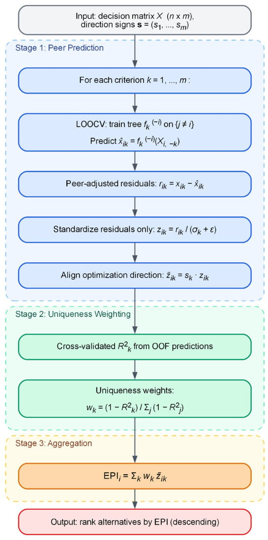
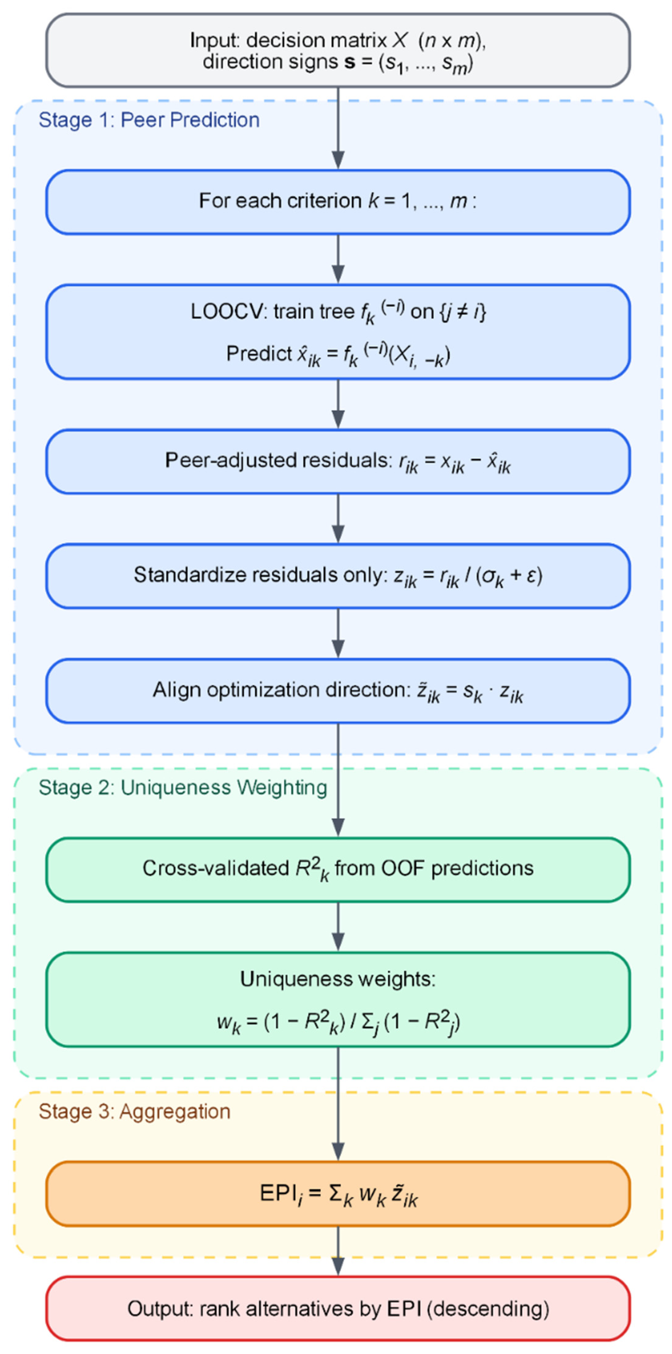
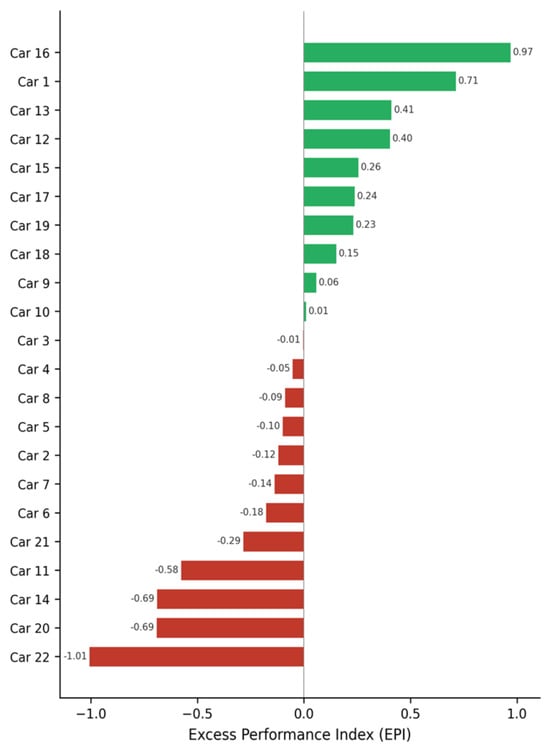
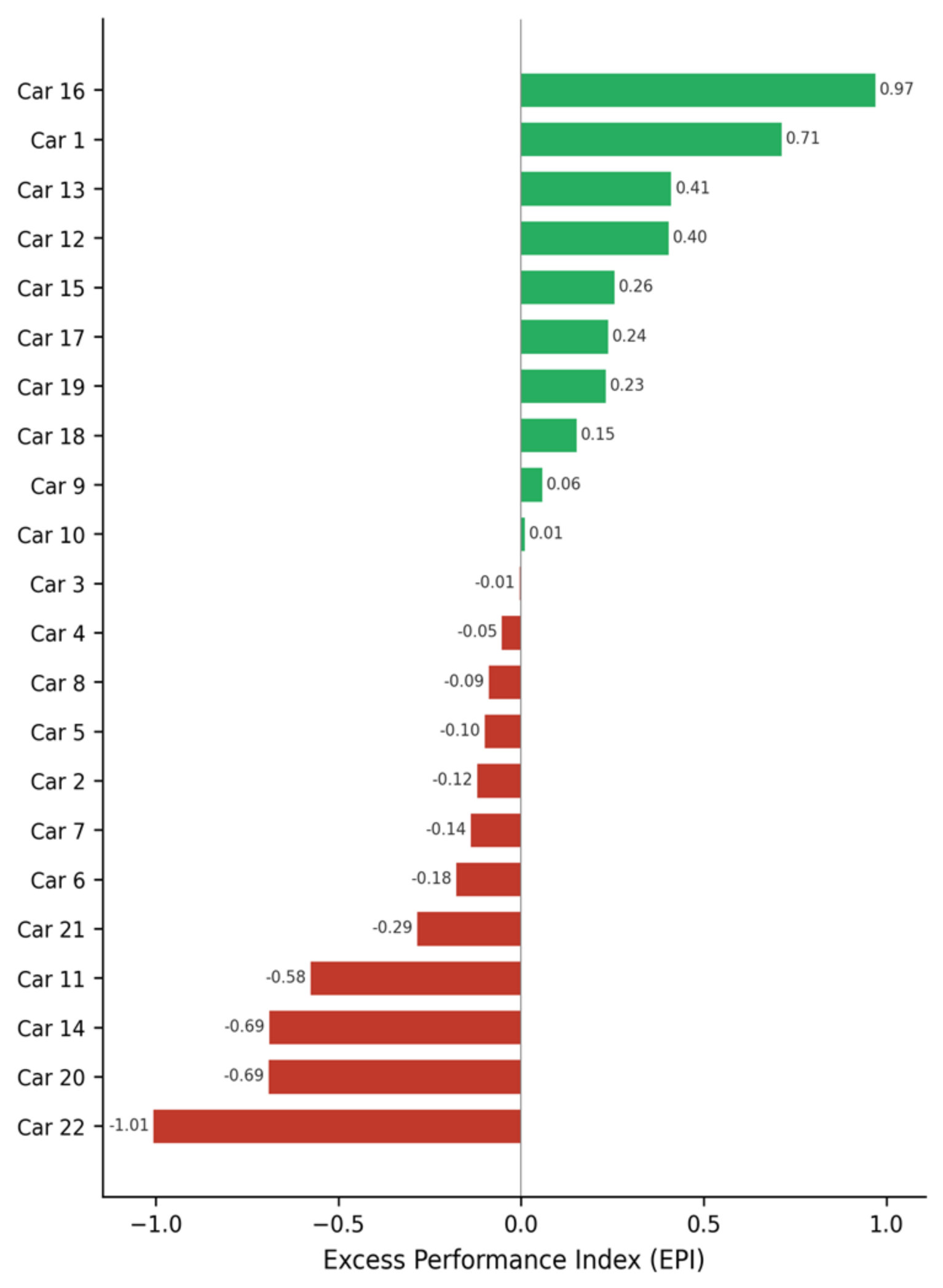
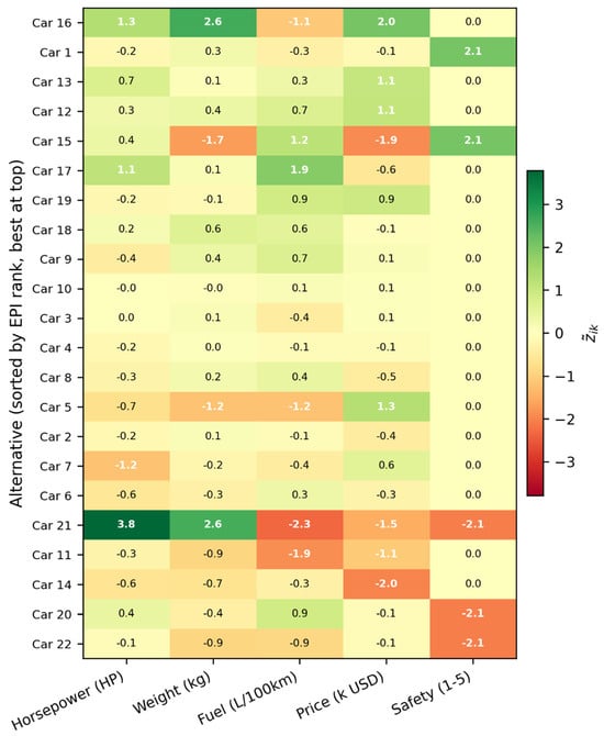
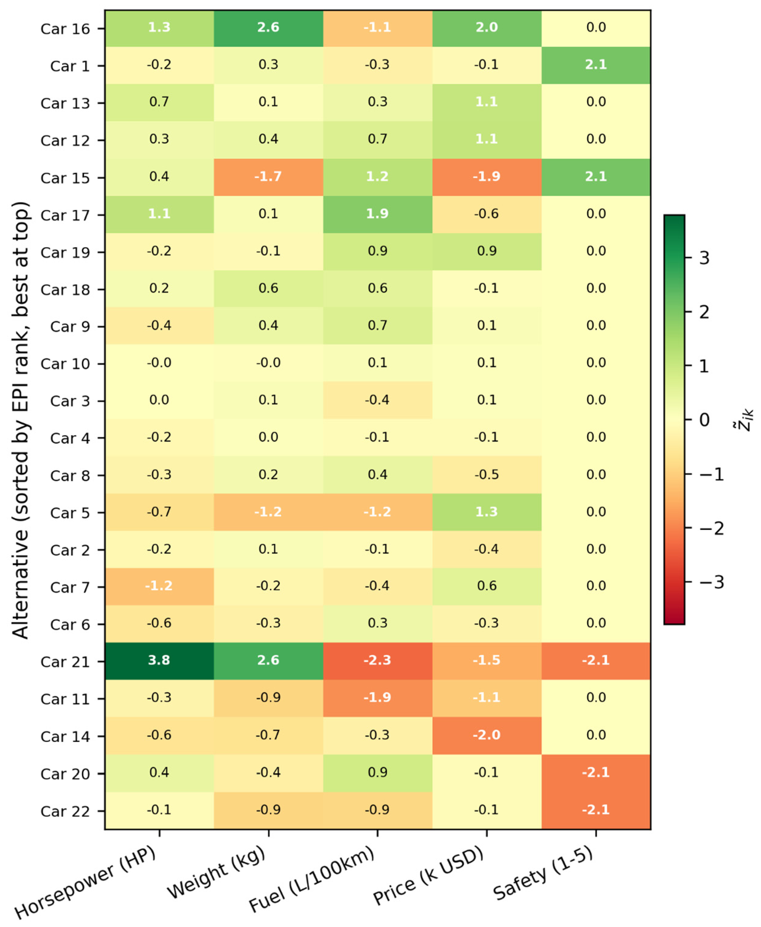
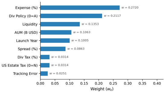
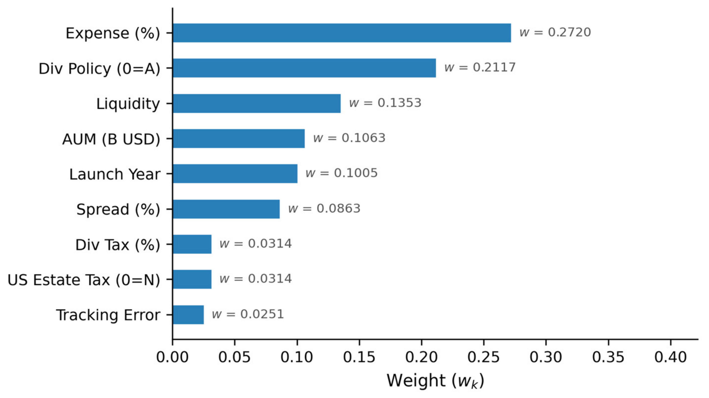
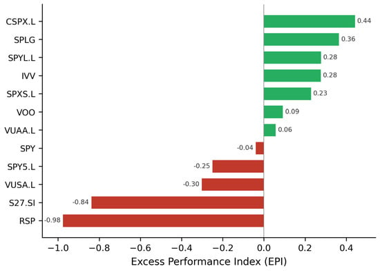
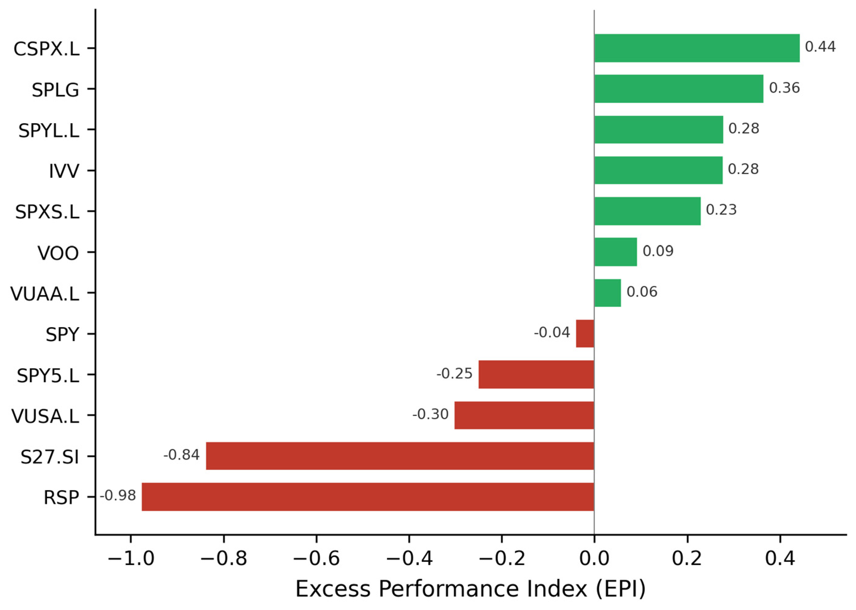
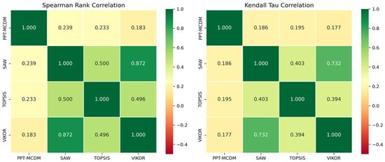
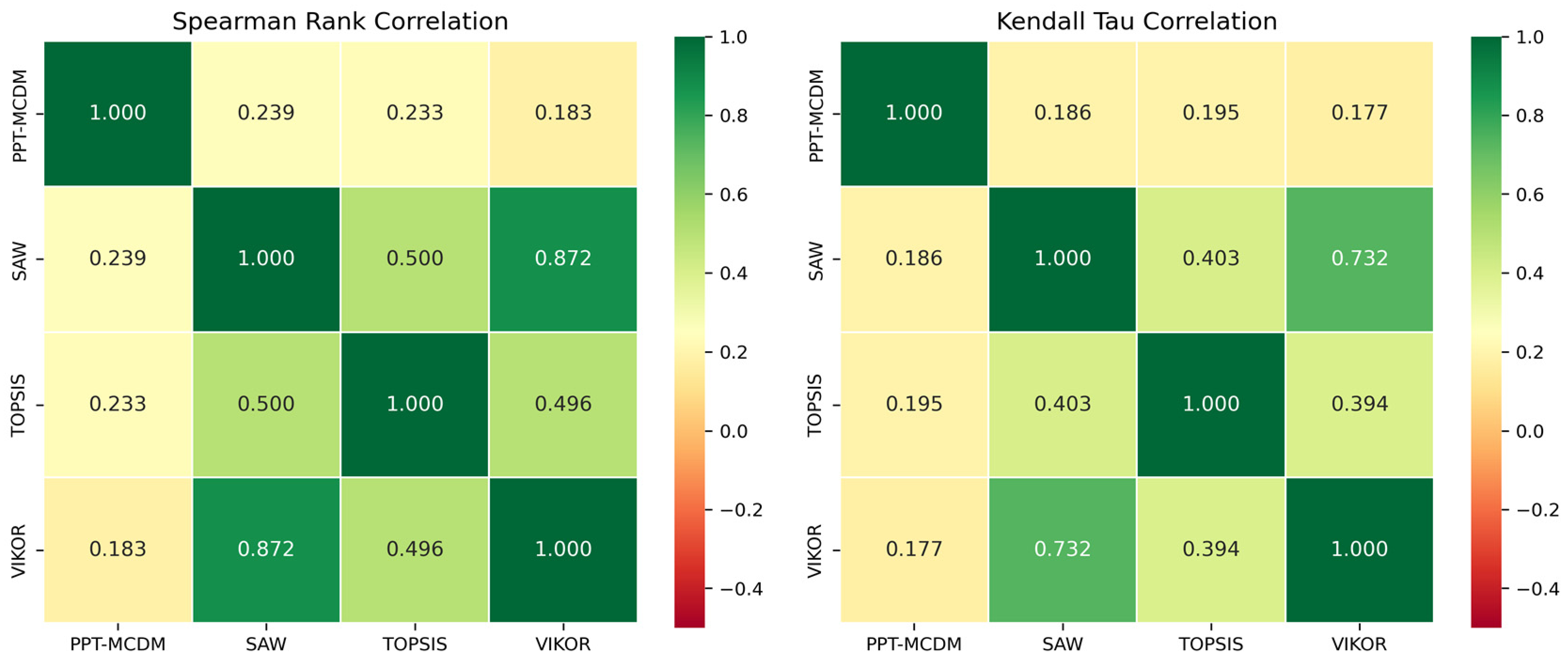
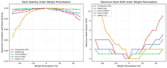
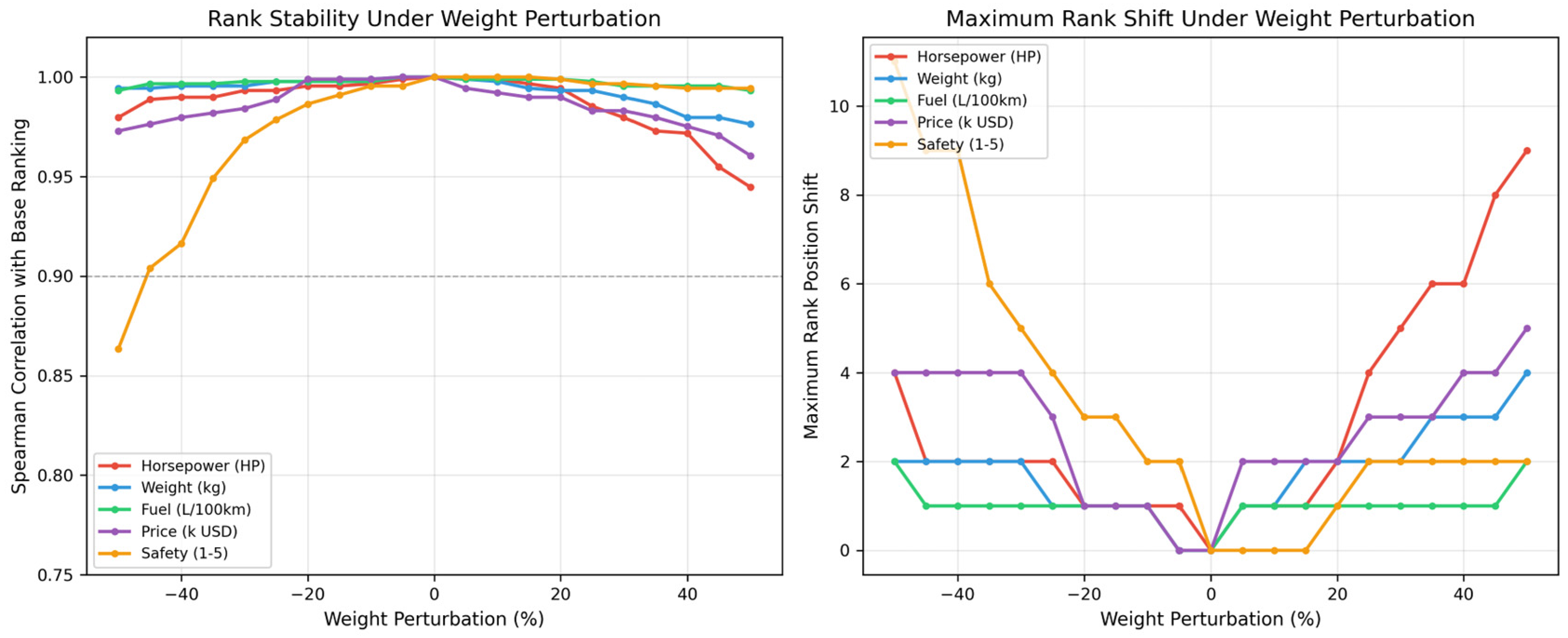
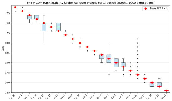
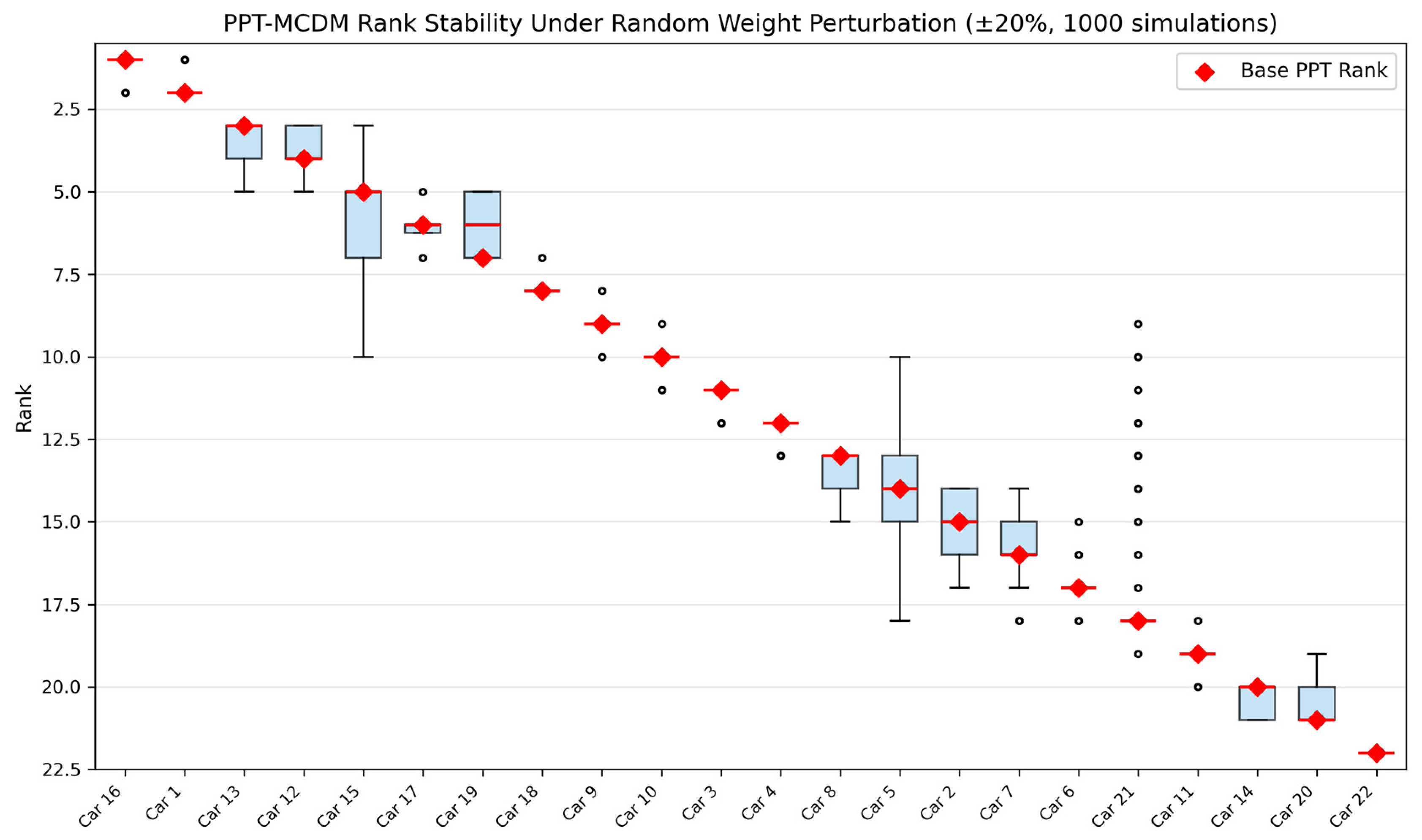

Disclaimer/Publisher’s Note: The statements, opinions and data contained in all publications are solely those of the individual author(s) and contributor(s) and not of MDPI and/or the editor(s). MDPI and/or the editor(s) disclaim responsibility for any injury to people or property resulting from any ideas, methods, instructions or products referred to in the content. |
© 2026 by the authors. Licensee MDPI, Basel, Switzerland. This article is an open access article distributed under the terms and conditions of the Creative Commons Attribution (CC BY) license.