An Enhanced Newton Downhill Optimizer for High-Dimensional Optimization and Thermal–Pumped-Storage Economic Dispatch

Abstract

The Newton Downhill Optimizer (NDO) provides a compact derivative-free search framework, but its random dimension mask, uniform treatment of individuals, and limited use of supplementary global-best candidates may restrict performance on high-dimensional problems. This study proposes an Enhanced Newton Downhill Optimizer (ENDO) that incorporates three mechanisms: an adaptive dimension mask, a DE/rand/2-based greedy mutation for inferior individuals, and dynamic-boundary opposition-based best guidance. ENDO was evaluated on the CEC2017 benchmark at 10, 30, 50, and 100 dimensions. The primary comparison involved nine representative optimizers, and an additional 100-dimensional comparison was conducted with six advanced optimizers. In the primary 100-dimensional tests, ENDO ranked first on 18 of 29 functions, remained among the top three on 26 functions, and achieved an average rank of 1.79. In the additional comparison, ENDO ranked third with an average rank of 3.52. Across the four dimensions, its average ranks were 1.79, 1.66, 1.38, and 1.79, indicating stable performance under changes in problem scale. ENDO was further applied to a 168-dimensional thermal–pumped-storage economic dispatch problem, where it achieved the lowest mean operating cost, the best average rank of 1.87, and a feasibility rate of 100% over 30 independent runs. Statistical analyses further supported the competitiveness of ENDO across the benchmark and engineering evaluations. These results show that ENDO improves the sustained search capability of NDO and provides competitive performance for complex high-dimensional and constrained optimization problems.

1. Introduction

1.1. Research Background and Motivation

Optimization is central to engineering design, energy management, production scheduling, parameter identification, and resource allocation. Many practical problems are high-dimensional, nonlinear, multimodal, and strongly constrained. Their objective functions may also be nonconvex, discontinuous, or unavailable in analytical form, which limits methods that depend on gradient information or specific mathematical structures. Metaheuristic algorithms address these difficulties through stochastic population search and have, therefore, become widely used in complex engineering optimization [1,2,3].

The performance of a metaheuristic largely depends on the balance between exploration and exploitation. Broad exploration is required to identify promising regions, whereas effective exploitation is needed to improve solutions once such regions have been found. Excessive concentration may lead to premature convergence, while persistent random search may slow late-stage refinement. According to the no free lunch theorem, no optimizer is uniformly superior across all problem classes [4]. Algorithm improvement should therefore be guided by the search characteristics of the underlying method rather than by simply adding unrelated strategies.

Thermal–pumped-storage economic dispatch is a representative high-dimensional constrained problem. Thermal-unit outputs and pumped-storage power must be coordinated over multiple periods while satisfying power balance, generation limits, ramping constraints, reserve requirements, storage bounds, and terminal energy conditions. The storage state links decisions across time, and a low-cost solution is not necessarily feasible. A suitable optimizer must therefore provide both competitive operating costs and reliable constraint satisfaction.

This study focuses on the Newton Downhill Optimizer (NDO), a derivative-free population-based method that combines downhill-guided information with the stochastic scattering operator (SSO) and hybrid-guided operator (HGO) [5]. NDO has a compact search structure, but three aspects remain open to improvement. Its dimension mask is generated from a random threshold without iteration-dependent regulation; inferior individuals receive no dedicated refinement after the main update; and the global best is mainly selected from candidates accepted through SSO and HGO.

To address these issues, an Enhanced Newton Downhill Optimizer, termed ENDO, is proposed. ENDO introduces an adaptive dimension mask, a DE/rand/2-based greedy mutation for inferior individuals, and dynamic-boundary opposition-based best guidance. The three mechanisms are placed at different stages of the NDO procedure to regulate dimension-wise updating, improve lower-ranked solutions, and enlarge the candidate pool used to update the global best.

1.2. Related Work

1.2.1. Metaheuristic Optimization Algorithms

Particle swarm optimization (PSO) updates each particle using its personal best position and the best position found by the swarm [6]. Its simple structure and limited number of control parameters have supported extensive applications and theoretical studies [7]. However, rapid attraction toward the current best positions may reduce population diversity on complex multimodal problems.

The grey wolf optimizer (GWO) models the leadership hierarchy and cooperative hunting behavior of grey wolves [8]. The three best solutions are treated as the α, β, and δ wolves, and the remaining individuals update their positions according to these leaders. A decreasing control parameter governs the transition between global search and local convergence. Although GWO is computationally simple, its reliance on a small number of leaders may accelerate population concentration.

The sparrow search algorithm (SSA) separates the population into producers, scroungers, and warning individuals, each with a different update rule [9]. The slime mould algorithm (SMA) uses adaptive weights and feedback mechanisms to simulate oscillatory foraging behavior [10]. Both methods introduce population heterogeneity, but their effectiveness may still vary with dimensionality and landscape structure.

Recent algorithms have adopted more specialized search models. Escape (ESC) represents calm, herding, and panic behaviors during crowd evacuation [11]. The artificial lemming algorithm (ALA) combines migration, burrowing, foraging, and predator-avoidance behaviors [12]. Stochastic social learning optimization (SSLO) uses observation, imitation, knowledge accumulation, and bucket theory to update weak solution components [13]. The detective behavior algorithm (DBA) organizes large-area investigation, local examination, and target tracking into successive search stages [14].

Unlike these biologically inspired methods, NDO derives its search direction from positional and fitness information. It combines the current solution, the global best, randomly sampled individuals, and downhill-guided information through SSO and HGO [5]. This structure is suitable for derivative-free optimization, but it does not explicitly regulate the dimension mask over time or assign additional search effort according to population quality.

1.2.2. Improvement Strategies for Metaheuristic Algorithms

Adaptive control is commonly used to vary search behavior during optimization. Early iterations usually require wider exploration, whereas later iterations benefit from more focused refinement. Iteration-dependent probabilities, weights, and control parameters can support this transition more effectively than fixed settings.

Differential evolution (DE) generates candidate solutions from scaled differences between population members [15]. These differences contain information about the current population distribution and can provide useful search directions in continuous spaces. Self-adaptive DE further adjusts its control parameters during the search, reducing sensitivity to fixed parameter values [16]. Nevertheless, applying differential mutation to every individual may disturb high-quality solutions. Selective mutation combined with greedy acceptance is more suitable when the objective is to refine only the inferior portion of the population.

Opposition-based learning (OBL) evaluates a solution together with an opposite candidate to increase the probability of sampling a promising region [17]. It has been incorporated into DE and other metaheuristics during initialization and population updating [18]. Generalized, quasi-oppositional, centroid-based, and population-dependent variants have since been developed [19]. Their performance depends on the boundary definition, insertion stage, and replacement rule.

Opposite points generated from fixed bounds may become less informative after the population has contracted into a smaller region. Dynamic bounds based on the current population can provide candidates that better reflect the active search area. In addition, using opposite candidates only for global-best updating can exploit new information without directly disturbing the accepted population.

Adaptive control, differential mutation, and opposition-based sampling, therefore, address different weaknesses: search-stage regulation, inferior-solution refinement, and candidate-space expansion, respectively. Their effectiveness depends on how they are integrated with the original algorithm. In ENDO, each mechanism has a separate role and a clearly defined execution stage.

1.2.3. Metaheuristic Algorithms for Economic Dispatch

Economic dispatch allocates generation among available units while minimizing operating cost and satisfying system constraints. Conventional formulations can often be solved efficiently when the objective is smooth and convex. Practical features, such as valve-point effects, prohibited operating regions, ramping limits, reserve requirements, and nonsmooth costs, make the problem more difficult.

PSO has been applied to economic dispatch with generator constraints [20], and improved variants have been developed for nonconvex dispatch models [21]. Differential evolution and hybrid optimization methods have also been used for dispatch problems with valve-point effects and nonsmooth generation costs [22]. These studies show that population-based methods can handle complex cost functions without analytical derivatives.

The inclusion of hydropower or energy storage introduces temporal coupling. Short-term hydrothermal scheduling requires the allocation of limited water or stored energy over multiple periods [23]. Generic storage models must represent charging, discharging, energy balance, efficiency losses, and terminal storage requirements [24].

Pumped-storage units can absorb power during low-load periods and generate during high-load periods. They have been incorporated into multi-region dynamic economic dispatch [25], day-ahead multi-source scheduling [26], and unit-commitment and market-dispatch models [27]. Their participation can improve system flexibility, but it also increases the number of decision variables and constraints.

A low penalized fitness does not necessarily imply a feasible dispatch schedule. Small violations of power balance, ramping, reserve, or storage constraints may remain if constraint handling is inadequate. Evaluation should therefore consider operating cost, feasibility rate, repeated-run variability, convergence behavior, constraint residuals, and runtime rather than a single best result.

1.3. Research Gaps and Motivation

The original NDO has three limitations relevant to high-dimensional optimization.

First, its binary dimension mask is generated using a random threshold that is independent of the iteration process. The contribution of different update components is therefore not explicitly adjusted as the search progresses.

Second, all individuals rely mainly on the SSO or HGO update. Lower-ranked individuals receive no additional refinement after the main population update, even though they may contain useful differential information or remain trapped in poor regions.

Third, the global best is updated primarily from candidates generated and accepted during the main search. The current population range is not used to construct supplementary candidates for global-best selection.

Another limitation in many algorithm studies is that performance is evaluated at only one dimension or only on unconstrained benchmarks. Such results provide limited evidence of scalability or engineering applicability. Cross-dimensional tests and a constrained scheduling problem are therefore included in this work.

ENDO is designed around these gaps. The adaptive mask regulates dimension-wise participation during the search. The DE/rand/2-based greedy mutation provides an additional search opportunity for inferior individuals. The dynamic-boundary opposition mechanism generates supplementary candidates for global-best updating without directly replacing population members.

1.4. Main Contributions

The main contributions of this study are as follows:

• An adaptive dimension mask is introduced into NDO. Its activation probability changes with the iteration, gradually modifying the contribution of the random-individual, global-best, and differential terms.
• A DE/rand/2-based greedy mutation is applied to lower-ranked individuals after the main update. A mutated candidate is accepted only when it improves the current solution, while higher-ranked individuals remain unchanged.
• A dynamic-boundary opposition-based guidance mechanism is developed. Opposite candidates are generated from the dimension-wise range of the current population and are used only to update the global best.
• ENDO is evaluated on the CEC2017 benchmark at 10, 30, 50, and 100 dimensions. The primary comparison includes nine representative optimizers, while an additional 100-dimensional comparison is conducted with six advanced optimizers: CMA-ES, SHADE, L-SHADE, LSHADE-SPACMA, EBOwithCMAR, and jSO. Solution quality, convergence, stability, statistical significance, and cross-dimensional performance are examined.
• Computational complexity, function-evaluation budget, parameter sensitivity, and population dynamics are analyzed to examine the computational characteristics and contributions of the proposed mechanisms.
• ENDO is applied to a 168-dimensional thermal–pumped-storage economic dispatch problem. The analysis covers operating cost, feasibility rate, constraint satisfaction, scheduling behavior, and computational efficiency.

1.5. Organization of the Paper

The remainder of this paper is organized as follows. Section 2 presents the basic NDO and the proposed ENDO. Section 3 reports the CEC2017 benchmark results and cross-dimensional analysis. Section 4 formulates the thermal–pumped-storage economic dispatch problem and discusses the scheduling results. Section 5 concludes the study.

2. Proposed Methodology

2.1. Basic Newton Downhill Optimizer

The Newton Downhill Optimizer (NDO) generates candidate solutions using downhill-guided information, the stochastic scattering operator (SSO), and the hybrid-guided operator (HGO) [5]. Boundary control and greedy selection are subsequently applied to update the population. NDO does not require analytical gradients and is therefore applicable to complex black-box optimization problems.

Let N denote the population size, D the problem dimension, t the current iteration, and T the maximum number of iterations. The i-th solution at iteration t is denoted by $p_i^t=\left[p_{i,1}^t,p_{i,2}^t,\dots ,p_{i,D}^t\right]$, where $p_{i,j}^t$ is its j-th component. The current global-best solution and its fitness are denoted by $p_{\mathrm{best}}^t$ and $f_{\mathrm{best}}^t=f\left(p_{\mathrm{best}}^t\right)$, respectively.

2.1.1. Population Initialization and Downhill-Guided Information

NDO randomly generates the initial population within the search bounds, as shown in Equation (1).

$$p_{i,j}=L_j+{\xi }_{i,j}\left(U_j-L_j\right), {\xi }_{i,j}~U\left(0,1\right)$$

(1)

where $L_j$ and $U_j$ denote the lower and upper bounds of the j-th dimension, respectively.

After initialization, all individuals are evaluated, and the current global-best individual is identified. The downhill-guided position vector is calculated from the current individual, the global-best individual, and their fitness values, as shown in Equation (2).

$$d_i^t=p_{\mathrm{best}}^t-{\xi }_{2,i}^t\left(1-{\xi }_{1,i}^t\right){\displaystyle \frac{f\left(p_i^t\right)}{f_{\mathrm{best}}^t-f\left(p_i^t\right)}}\left(p_{\mathrm{best}}^t-p_i^t+\epsilon 1_D\right)$$

(2)

where ${\xi }_{1,i}^t,{\xi }_{2,i}^t\sim U(0,1)$ are independent random numbers, $d_i^t$ is the downhill-guided position vector, $1_D$ is a D-dimensional vector of ones, and $\epsilon$ denotes the machine-precision constant. Equation (2) defines the downhill-guided calculation adopted in NDO.

2.1.2. Stochastic Scattering and Hybrid-Guided Operators

The basic NDO generates a random binary dimension mask for each individual, where $m_{i,j}^t=\mathbb{I}\left({\mu }_{i,j}^t>{\rho }_i^t\right)$, and both ${\mu }_{i,j}^t$ and ${\rho }_i^t$ follow the uniform distribution over [0, 1]. The same threshold ${\rho }_i^t$ is shared by all dimensions of the individual. SSO is selected with a probability of 0.5, and the candidate solution is generated using Equation (3).

$$q_i^t=m_i^t\odot p_i^t+\left(1_D-m_i^t\right)\odot \left[p_{\mathrm{best}}^t+u_{1,i}^t\odot \left(p_{a_2}^t-p_{a_3}^t\right)\right]+d_i^t{e}^{-t}\left|{\displaystyle \frac{f\left(p_{a_2}^t\right)}{f\left(p_{a_3}^t\right)+\epsilon }}\right|$$

(3)

where $q_i^t$ is the candidate solution, $u_{1,i}^t$ is a random vector uniformly distributed in ${\left[0,1\right]}^D$, $a_2$ and $a_3$ are independently sampled population indices, and $\odot$ denotes the Hadamard product. $p_{a_2}^t$ and $p_{a_3}^t$ denote the currently stored positions of the randomly selected individuals during iteration t.

Otherwise, HGO is applied, and one of the two update rules in Equation (4) is selected with equal probability.

$$q_i^t=\left\{\begin{array}{ll}{d}_i^t\odot u_{2,i}^t+\left(1_D-u_{3,i}^t\right)\odot p_i^t+m_i^t\odot p_{a_1}^t,\hfill & {\delta }_i^t<0.5,\hfill \\ p_{\mathrm{best}}^t\odot u_{4,i}^t+u_{5,i}^t\odot \left[p_{\mathrm{best}}^t\odot d_i^t\odot u_{6,i}^t-p_i^t\right],\hfill & {\delta }_i^t\ge 0.5.\hfill \end{array}\right.$$

(4)

Here, $u_{2,i}^t,\cdots ,u_{6,i}^t$ are independent random vectors, ${\delta }_i^t\sim U(0,1)$, and $a_1$ is a randomly sampled population index. The first rule combines the downhill-guided position, current individual, and mask-controlled random individual, whereas the second rule generates a candidate through element-wise coupling between the global-best and downhill-guided positions [5].

2.1.3. Boundary Control and Greedy Selection

Candidate solutions generated by SSO or HGO may exceed the search bounds. Each infeasible component is randomly regenerated within its corresponding feasible interval, as shown in Equation (5).

$${\tilde{q}}_{i,j}^t=\left\{\begin{array}{ll}{L}_j+{\zeta }_{i,j}^t\left(U_j-L_j\right),\hfill & q_{i,j}^t<L_j \mathrm{or} q_{i,j}^t>U_j,\hfill \\ q_{i,j}^t,\hfill & \mathrm{otherwise}.\hfill \end{array}\right.$$

(5)

where ${\zeta }_{i,j}^t\sim U(0,1)$, and ${\tilde{q}}_i^t$ denotes the candidate solution after boundary control. Unlike boundary clipping, this mechanism randomly regenerates each infeasible component within its feasible interval.

Greedy selection is then performed using Equation (6):

$$p_i^t\leftarrow \left\{\begin{array}{ll}{\tilde{q}}_i^t,\hfill & f\left({\tilde{q}}_i^t\right)\le f\left(p_i^t\right),\hfill \\ p_i^t,\hfill & \mathrm{otherwise}.\hfill \end{array}\right.$$

(6)

The candidate solution is accepted when its fitness is not greater than that of the current individual; otherwise, the pre-update position is retained. If the fitness of the accepted individual is not greater than the current global-best fitness, the global-best position and fitness are updated accordingly.

2.2. Enhanced Newton Downhill Optimizer

The random dimension mask of the basic NDO lacks iteration-dependent regulation, while inferior individuals receive no additional search after the main update. Moreover, the global-best information is mainly obtained from candidates generated and accepted by SSO and HGO. To address these limitations, an Enhanced Newton Downhill Optimizer (ENDO) is proposed. ENDO retains the main NDO framework and incorporates an adaptive dimension mask, DE/rand/2-based greedy mutation for inferior individuals, and dynamic-boundary opposition-based best guidance.

2.2.1. Adaptive Dimension Mask

The basic NDO generates its dimension mask using a random threshold, and the mask activation ratio is not regulated by the iteration process. ENDO replaces the random threshold with an iteration-dependent linear threshold. The adaptive dimension mask is defined in Equation (7):

$$m_{i,j}^t=\mathbb{I}\left({\mu }_{i,j}^t>0.3+0.4{\displaystyle \frac{t}{T}}\right), {\mu }_{i,j}^t~U\left(0,1\right)$$

(7)

According to Equation (7), the mask threshold increases linearly from 0.3 to 0.7, corresponding to a decrease in the activation probability from 0.7 to 0.3 as the iteration proceeds. The linear schedule provides a gradual transition in dimensional participation without introducing additional shape or feedback parameters. In SSO, activated dimensions retain the current-position term, whereas inactive dimensions receive global-best and differential guidance. The downhill-guided term is applied to all dimensions. Consequently, global-best and differential information affects more dimensions in the later search stage. In the first HGO rule, the mask controls the random-individual term $m_i^t\odot p_{a_1}^t$, and its decreasing activation probability gradually reduces the contribution of this term. The second HGO rule does not use the mask.

2.2.2. DE/Rand/2-Based Greedy Mutation for Inferior Individuals

After the SSO/HGO update, ENDO sorts the population in ascending order of fitness. Individuals ranked from $⌈0.7N⌉$ to N are selected for further refinement. The value of 0.7 was selected to focus the additional mutation on approximately the worst 30% of the population while avoiding unnecessary disturbance to better-performing individuals. Let ${\pi }^t\left(k\right)$ denote the index of the individual ranked k-th. The selected subset is defined as ${\mathcal{I}}_{\mathrm{poor}}^t=\left\{{\pi }^t\left(k\right)\mid k=⌈0.7N⌉,\dots ,N\right\}$. For each $i\in {\mathcal{I}}_{\mathrm{poor}}^t$, a DE/rand/2-based mutation is performed with a probability of 0.5, as shown in Equation (8):

$$v_i^t=\left\{\begin{array}{ll}{p}_{r_1}^t+F_i^t\left(p_{r_2}^t-p_{r_3}^t\right)+F_i^t\left(p_{r_4}^t-p_{r_5}^t\right),\hfill & {\chi }_i^t>0.5,\hfill \\ p_i^t,\hfill & {\chi }_i^t\le 0.5.\hfill \end{array}\right.$$

(8)

Here, ${\chi }_i^t$, $F_i^t\sim U(0,1)$, and $r_1,\dots ,r_5$ are sampled independently with replacement. Repeated indices are therefore possible. For N = 30, the probability of at least one repeated index is 29.63%, whereas complete cancellation of the combined differential term due solely to index coincidence occurs with a probability of 0.2185% when the mutation branch is activated. Thus, index repetition may reduce the differential perturbation but does not generally eliminate it. The same random scaling factor $F_i^t$ is applied to both differential vectors.

The mutated candidate is clipped using ${\tilde{v}}_{i,j}^t=\min \left\{U_j,\max \left\{L_j,v_{i,j}^t\right\}\right\}$. Unlike the main NDO update, which employs random regeneration for infeasible components, the mutation-based candidate adopts boundary clipping. This difference is determined by the characteristics of the two search operators. Random regeneration in the main update maintains stochastic exploration after large position changes, whereas clipping in DE/rand/2 mutation preserves the directional information contained in the differential vector. Therefore, the two boundary-handling strategies serve different purposes and are retained separately in ENDO. It replaces the current individual only when $f\left({\tilde{v}}_i^t\right)<f\left(p_i^t\right)$. This strategy applies additional differential search only to the selected inferior individuals without directly modifying the higher-ranked individuals.

2.2.3. Dynamic-Boundary Opposition-Based Best Guidance

After the DE/rand/2-based greedy mutation, ENDO constructs opposite candidates using the dimension-wise range of the current population. The dynamic lower and upper bounds of the j-th dimension are $p_j^{\min ,t}={\min }_i{p}_{i,j}^t$ and $p_j^{\max ,t}={\max }_i{p}_{i,j}^t$, respectively. Based on these dynamic bounds, the opposite component associated with the i-th individual is generated using Equation (9):

$$p_{i,j}^{\mathrm{opp},t}=p_j^{\max ,t}+p_j^{\min ,t}-p_{i,j}^t$$

(9)

Each opposite candidate is checked against the search bounds and then evaluated. If a better solution is obtained, the global-best position and fitness are updated. Although the dynamic interval may shrink during later iterations, opposite candidates are only used as additional candidates rather than replacing the current population directly. Therefore, the contraction of the opposite search range does not cause population collapse, but only affects the contribution of opposition learning during the exploitation stage.

2.2.4. Overall Procedure of ENDO

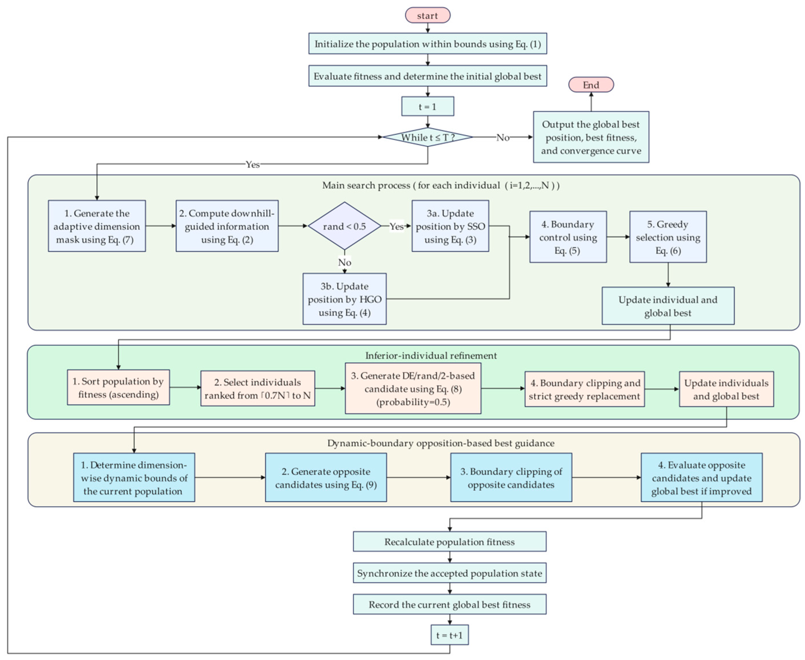
The overall procedure of ENDO is illustrated in Figure 1. The population is first initialized using Equation (1). All individuals are then evaluated, and the initial global-best individual is identified. During each iteration, the adaptive dimension mask is generated using Equation (7), and the downhill-guided position vector is calculated using Equation (2). SSO in Equation (3) is selected with a probability of 0.5; otherwise, HGO is performed using one of the update rules in Equation (4).

After a candidate individual is generated, infeasible components are handled using Equation (5), followed by the greedy selection in Equation (6) and the update of the global-best information. Once the main update of all individuals is completed, the population is sorted in ascending order of fitness. Individuals ranked from $⌈0.7N⌉$ to N undergo the DE/rand/2-based greedy mutation defined in Equation (8). Dynamic opposite candidates are subsequently generated using Equation (9) based on the dimension-wise range of the current population, and better opposite candidates are used to update the global-best information.

Finally, all N individuals in the current population are re-evaluated to update their fitness values. The accepted population is then synchronized, and the current global-best fitness is recorded. When the maximum number of iterations is reached, the global-best position, best fitness, and convergence curve are returned; otherwise, the next iteration begins.

2.2.5. Computational Complexity Analysis

The computational complexity of ENDO is mainly determined by the population update, sorting, mutation, and opposition-based search. For a population of N individuals in a D-dimensional search space, the main NDO update requires $O(ND)$ operations per iteration. Ranking the population requires $O(N\log N)$, while the greedy mutation of $N_{\mathrm{poor}}$ inferior individuals requires $O(N_{\mathrm{poor}}D)$. The dynamic-boundary opposition-based search requires $O(ND)$. Therefore, excluding the cost of objective-function evaluations, the overall computational complexity of ENDO over T iterations is $O\left(TND+TN\log N+T{N}_{\mathrm{poor}}D\right)$. Since $N_{\mathrm{poor}}\le N$, this can be simplified to $O\left(TND+TN\log N\right)$. Since $D\gg \log N$ in the high-dimensional setting considered in this study, the $O(TND)$ term dominates the computational cost. The additional mutation and opposition-based operations increase the constant computational cost. The corresponding increase in objective-function evaluations is analyzed separately in Section 3.2.6.

3. Experimental Results and Analysis

3.1. Benchmark Experimental Settings

The CEC2017 benchmark suite [28] was used to evaluate ENDO. The primary comparison included NDO, DBA, ESC, SSLO, SMA, SSA, ALA, PSO, and GWO. All algorithms used a population size of 30 and a maximum of 1000 iterations, and each test was repeated independently 30 times. The 100-dimensional case was used for the main evaluation, while the 10-, 30-, and 50-dimensional cases were used to assess scalability. The ablation and parameter-sensitivity experiments were conducted at 100 dimensions using the same population size, iteration limit, and number of independent runs.

To further evaluate ENDO against stronger optimizers, an additional 100-dimensional comparison was conducted with CMA-ES, SHADE, L-SHADE, LSHADE-SPACMA, EBOwithCMAR, and jSO [29,30,31,32,33,34], with ENDO and NDO included as references. For this comparison, all algorithms were evaluated according to the experimental settings adopted in this study, with N = 30, T = 1000, and 30 independent runs, rather than their original competition-specific settings. For algorithms involving population reduction or function-evaluation-based control, the implementations were adapted to the common N/T framework while retaining their main search mechanisms. The implementation details are summarized in

Table 1. Implementation settings of the advanced comparison algorithms under the unified experimental protocol.

Algorithm	Interpretation of N	Iteration/Progress Control	Retained Algorithm-Specific Mechanisms
SHADE	Fixed population size, N = 30	T = 1000 generations	Success-history adaptation of F and CR, p-best mutation, and external archive
L-SHADE	Initial population size, N = 30, reduced to 4	T = 1000 generations; population reduction scheduled by iteration progress	SHADE parameter adaptation, p-best mutation, external archive, and linear population-size reduction
LSHADE-SPACMA	Initial population size, N = 30, reduced to 4	T = 1000 generations; iteration-based population reduction	L-SHADE mechanisms, adaptive hybridization, and CMA-based search
jSO	Initial population size, N = 30, reduced to 4	T = 1000 generations; FE-dependent schedules mapped to normalized iteration progress	jSO-specific F/CR adaptation, p-best selection, external archive, and linear population-size reduction
CMA-ES	Offspring population size, λ = N = 30	T = 1000 generations	Covariance-matrix adaptation and step-size adaptation
EBOwithCMAR	Total initial population, N = 30	T = 1000 outer iterations; progress-dependent controls expressed by iteration progress	EBO and CMAR/CMA search, information sharing, and population reduction

Note: N denotes the population parameter supplied by the unified experimental framework, and T denotes the prescribed iteration limit. The interpretation of N follows the internal structure of each algorithm rather than forcing a fixed population of 30 throughout the search. FE denotes function evaluation; CMA denotes covariance matrix adaptation; CMAR denotes covariance matrix adapted retreat; and EBO denotes Effective Butterfly Optimizer.

.

Since the implementations require different numbers of objective-function evaluations, the unified N/T protocol does not imply an identical FE budget. The exact FE budgets were also recorded. Under the above settings, ENDO requires 190,030 FEs; NDO and DBA require 90,030 FEs; SSA requires 39,030 FEs; ESC, SSLO, and ALA require 30,030 FEs; and SMA, PSO, and GWO require 30,000 FEs. These counts are unchanged across the four-dimensional settings because the population size and iteration limit remain fixed. To assess the effect of the unequal evaluation budgets, an FE-matched experiment was conducted at 100 dimensions. An extended-budget NDO variant, denoted as NDO-FE, retained the original NDO search operators but used 190,020 FEs, closely matching the 190,030 FEs of ENDO. The corresponding analysis is presented in Section 3.2.6.

The minimum value (Min), mean value (Avg), and standard deviation (Std) were obtained from the 30 independent runs. Ranking was based primarily on the mean fitness value, with a smaller mean indicating a better rank. When the mean values were identical, the standard deviation was used as the secondary criterion. Algorithms with identical mean and standard deviation values were assigned the same rank. Statistical significance was examined using the Wilcoxon rank-sum test [35] at α = 0.05. For the primary comparison, overall differences among the ten algorithms were further assessed using the Friedman test, followed by Holm-corrected post hoc comparisons with ENDO as the control algorithm. The same procedure was applied separately to the advanced comparison.

3.2. Comprehensive Performance Analysis at 100 Dimensions

To provide a structured assessment of ENDO in high-dimensional optimization, the 100-dimensional results are examined in terms of overall solution quality, convergence behavior, stability, and statistical significance.

3.2.1. Overall Performance Analysis

Table 2. Statistical results of the compared algorithms on the 100-dimensional CEC2017 functions F₁ and F₃–F₁₀.

f	Results	ENDO	NDO	DBA	ESC	SSLO	SMA	SSA	ALA	PSO	GWO
F1	min	1.10 × 107	9.92 × 108	7.39 × 105	3.36 × 1010	1.02 × 1010	3.38 × 107	2.89 × 107	1.29 × 109	4.17 × 1010	3.45 × 1010
	std	2.10 × 108	2.79 × 109	3.16 × 105	1.17 × 1010	1.16 × 109	1.42 × 107	5.32 × 107	1.36 × 109	1.24 × 1010	8.98 × 109
	avg	7.53 × 107	4.88 × 109	1.39 × 106	5.13 × 1010	1.36 × 1010	5.53 × 107	9.54 × 107	2.76 × 109	6.11 × 1010	5.59 × 1010
	rank	3	6	1	8	7	2	4	5	10	9
F3	min	2.19 × 105	3.95 × 105	1.81 × 105	4.15 × 105	4.41 × 105	2.33 × 105	3.29 × 105	1.81 × 105	3.43 × 105	3.22 × 105
	std	4.82 × 104	6.56 × 104	1.20 × 104	5.34 × 104	6.32 × 104	2.19 × 105	5.79 × 104	2.97 × 104	1.36 × 105	7.43 × 104
	avg	3.20 × 105	5.34 × 105	2.03 × 105	5.26 × 105	5.98 × 105	4.98 × 105	4.97 × 105	2.52 × 105	5.48 × 105	4.26 × 105
	rank	3	8	1	7	10	6	5	2	9	4
F4	min	7.74 × 102	1.11 × 103	6.38 × 102	3.68 × 103	2.26 × 103	7.52 × 102	8.74 × 102	1.08 × 103	4.70 × 103	3.37 × 103
	std	9.71 × 101	3.43 × 102	5.62 × 101	2.43 × 103	1.75 × 102	5.41 × 101	4.37 × 101	1.59 × 102	2.19 × 103	1.40 × 103
	avg	8.97 × 102	1.55 × 103	7.72 × 102	6.31 × 103	2.63 × 103	8.48 × 102	9.53 × 102	1.29 × 103	8.29 × 103	5.31 × 103
	rank	3	6	1	9	7	2	4	5	10	8
F5	min	7.66 × 102	9.79 × 102	1.23 × 103	8.63 × 102	1.31 × 103	1.12 × 103	1.26 × 103	1.04 × 103	1.25 × 103	1.06 × 103
	std	5.76 × 101	7.99 × 101	3.06 × 101	9.14 × 101	3.29 × 101	8.44 × 101	4.99 × 101	8.60 × 101	1.05 × 102	7.88 × 101
	avg	8.76 × 102	1.11 × 103	1.34 × 103	1.01 × 103	1.38 × 103	1.27 × 103	1.38 × 103	1.18 × 103	1.49 × 103	1.22 × 103
	rank	1	3	7	2	9	6	8	4	10	5
F6	min	6.05 × 102	6.23 × 102	6.64 × 102	6.13 × 102	6.22 × 102	6.45 × 102	6.63 × 102	6.34 × 102	6.61 × 102	6.35 × 102
	std	3.74 × 100	6.17 × 100	1.93 × 100	3.20 × 100	1.84 × 100	6.65 × 100	2.01 × 100	8.00 × 100	5.70 × 100	5.19 × 100
	avg	6.12 × 102	6.36 × 102	6.67 × 102	6.20 × 102	6.26 × 102	6.58 × 102	6.66 × 102	6.51 × 102	6.68 × 102	6.45 × 102
	rank	1	4	9	2	3	7	8	6	10	5
F7	min	1.15 × 103	1.80 × 103	2.98 × 103	1.38 × 103	2.34 × 103	1.93 × 103	3.03 × 103	1.78 × 103	2.55 × 103	1.96 × 103
	std	1.56 × 102	2.49 × 102	6.89 × 101	2.12 × 102	4.52 × 101	2.21 × 102	8.59 × 101	1.95 × 102	3.26 × 102	1.50 × 102
	avg	1.39 × 103	2.26 × 103	3.15 × 103	1.81 × 103	2.43 × 103	2.14 × 103	3.26 × 103	2.15 × 103	3.33 × 103	2.20 × 103
	rank	1	6	8	2	7	3	9	4	10	5
F8	min	1.07 × 103	1.27 × 103	1.60 × 103	1.20 × 103	1.61 × 103	1.38 × 103	1.74 × 103	1.31 × 103	1.66 × 103	1.41 × 103
	std	5.67 × 101	1.98 × 102	5.84 × 101	1.04 × 102	3.48 × 101	1.03 × 102	4.48 × 101	1.02 × 102	1.14 × 102	1.07 × 102
	avg	1.16 × 103	1.44 × 103	1.79 × 103	1.35 × 103	1.69 × 103	1.58 × 103	1.86 × 103	1.47 × 103	1.87 × 103	1.53 × 103
		1	3	8	2	7	6	9	4	10	5
F9	min	3.02 × 103	1.46 × 104	2.16 × 104	9.02 × 103	2.20 × 104	2.39 × 104	2.42 × 104	9.60 × 103	2.37 × 104	2.23 × 104
	std	6.18 × 103	1.44 × 104	1.63 × 103	4.89 × 103	4.70 × 103	4.66 × 103	4.04 × 102	9.59 × 103	5.79 × 103	1.18 × 104
	avg	1.42 × 104	3.38 × 104	2.65 × 104	1.81 × 104	3.26 × 104	3.32 × 104	2.48 × 104	3.37 × 104	3.25 × 104	3.99 × 104
		1	9	4	2	6	7	3	8	5	10
F10	min	1.29 × 104	1.80 × 104	1.48 × 104	2.57 × 104	2.04 × 104	1.39 × 104	1.53 × 104	1.86 × 104	1.55 × 104	1.43 × 104
	std	3.19 × 103	2.70 × 103	8.55 × 102	1.01 × 103	6.14 × 102	1.58 × 103	1.20 × 103	2.64 × 103	1.28 × 103	3.34 × 103
	avg	1.64 × 104	2.42 × 104	1.64 × 104	2.80 × 104	2.19 × 104	1.76 × 104	1.72 × 104	2.44 × 104	1.84 × 104	1.74 × 104
		1	8	2	10	7	5	3	9	6	4

,

Table 3. Statistical results of the compared algorithms on the 100-dimensional CEC2017 functions F₁₁–F₂₀.

f	Results	ENDO	NDO	DBA	ESC	SSLO	SMA	SSA	ALA	PSO	GWO
F11	min	1.24 × 104	2.86 × 104	2.77 × 103	4.10 × 104	8.42 × 104	3.30 × 103	2.38 × 104	1.72 × 104	1.80 × 104	4.67 × 104
	std	1.76 × 104	1.96 × 104	3.48 × 102	1.58 × 104	1.60 × 104	2.13 × 103	1.83 × 104	7.41 × 103	1.93 × 104	1.76 × 104
	avg	2.68 × 104	6.61 × 104	3.39 × 103	6.74 × 104	1.16 × 105	6.28 × 103	5.63 × 104	2.66 × 104	4.49 × 104	7.65 × 104
	rank	4	7	1	8	10	2	6	3	5	9
F12	min	9.29 × 106	7.37 × 107	1.60 × 108	3.81 × 109	2.98 × 109	7.75 × 107	4.47 × 107	9.11 × 107	4.98 × 109	5.25 × 109
	std	1.64 × 107	5.24 × 108	4.78 × 107	3.74 × 109	3.74 × 108	1.12 × 108	5.34 × 107	9.94 × 107	6.54 × 109	7.46 × 109
	avg	3.25 × 107	3.43 × 108	2.32 × 108	7.70 × 109	3.52 × 109	2.52 × 108	1.31 × 108	2.36 × 108	1.20 × 1010	1.37 × 1010
	rank	1	6	3	8	7	5	2	4	9	10
F13	min	2.58 × 103	5.53 × 103	2.19 × 104	2.78 × 104	1.18 × 107	4.47 × 104	1.06 × 104	1.80 × 104	3.49 × 106	1.45 × 108
	std	3.05 × 103	6.29 × 103	7.72 × 103	7.69 × 108	1.26 × 107	1.60 × 106	2.51 × 105	1.67 × 104	1.53 × 109	1.58 × 109
	avg	6.15 × 103	1.50 × 104	3.50 × 104	5.49 × 108	2.93 × 107	9.20 × 105	7.86 × 104	4.36 × 104	9.89 × 108	1.74 × 109
	rank	1	2	3	8	7	6	5	4	9	10
F14	min	3.23 × 105	8.02 × 105	6.27 × 105	2.99 × 106	6.53 × 106	6.69 × 105	5.10 × 105	6.02 × 104	9.68 × 105	1.24 × 106
	std	8.43 × 105	1.05 × 106	2.22 × 105	3.97 × 106	7.00 × 106	1.49 × 106	7.95 × 105	4.59 × 105	3.49 × 106	4.71 × 106
	avg	1.50 × 106	2.04 × 106	1.04 × 106	8.82 × 106	1.77 × 107	2.87 × 106	1.86 × 106	4.97 × 105	3.97 × 106	7.79 × 106
	rank	3	5	2	9	10	6	4	1	7	8
F15	min	1.86 × 103	2.31 × 103	1.59 × 104	1.16 × 104	2.74 × 105	3.91 × 104	3.08 × 103	3.42 × 103	3.08 × 104	1.39 × 106
	std	1.70 × 104	3.54 × 103	8.01 × 103	1.83 × 108	1.49 × 106	4.20 × 105	5.79 × 103	1.98 × 104	4.53 × 108	5.17 × 108
	avg	7.16 × 103	5.34 × 103	2.81 × 104	7.52 × 107	2.37 × 106	2.70 × 105	1.07 × 104	1.54 × 104	2.35 × 108	3.41 × 108
	rank	2	1	5	8	7	6	3	4	9	10
F16	min	3.66 × 103	4.80 × 103	5.90 × 103	3.89 × 103	7.59 × 103	4.97 × 103	5.24 × 103	5.04 × 103	5.99 × 103	5.13 × 103
	std	6.78 × 102	6.79 × 102	7.88 × 102	1.18 × 103	3.10 × 102	6.09 × 102	6.65 × 102	8.68 × 102	1.01 × 103	6.60 × 102
	avg	5.19 × 103	5.83 × 103	7.49 × 103	6.53 × 103	8.14 × 103	6.18 × 103	6.47 × 103	6.60 × 103	7.53 × 103	6.46 × 103
	rank	1	2	8	6	10	3	5	7	9	4
F17	min	3.51 × 103	4.00 × 103	4.71 × 103	3.48 × 103	5.54 × 103	4.65 × 103	4.67 × 103	3.91 × 103	4.46 × 103	4.50 × 103
	std	6.74 × 102	5.53 × 102	5.55 × 102	6.70 × 102	3.57 × 102	5.31 × 102	5.80 × 102	7.21 × 102	2.07 × 104	1.42 × 103
	avg	4.72 × 103	5.06 × 103	5.97 × 103	4.81 × 103	6.41 × 103	5.56 × 103	6.05 × 103	5.81 × 103	1.02 × 104	5.74 × 103
	rank	1	3	7	2	9	4	8	6	10	5
F18	min	7.78 × 105	1.45 × 106	9.94 × 105	3.28 × 106	5.82 × 106	1.22 × 106	3.60 × 105	4.31 × 105	1.73 × 106	1.44 × 106
	std	1.31 × 106	1.84 × 106	3.30 × 105	7.71 × 106	6.97 × 106	3.45 × 106	1.23 × 106	8.07 × 105	2.90 × 106	6.80 × 106
	avg	2.83 × 106	3.93 × 106	1.65 × 106	1.21 × 107	2.03 × 107	7.86 × 106	2.32 × 106	1.07 × 106	6.06 × 106	7.73 × 106
	rank	4	5	2	9	10	8	3	1	6	7
F19	min	2.15 × 103	2.23 × 103	7.73 × 105	1.31 × 105	9.87 × 105	3.61 × 104	2.58 × 103	2.42 × 103	4.08 × 105	1.44 × 107
	std	1.95 × 103	5.93 × 103	1.64 × 106	1.96 × 108	3.80 × 106	1.45 × 105	8.20 × 103	7.05 × 103	3.40 × 108	2.52 × 108
	avg	4.17 × 103	7.69 × 103	3.15 × 106	5.86 × 107	4.26 × 106	2.06 × 105	9.13 × 103	9.56 × 103	1.98 × 108	2.15 × 108
	rank	1	2	6	8	7	5	3	4	9	10
F20	min	3.62 × 103	4.26 × 103	3.79 × 103	4.84 × 103	5.70 × 103	4.13 × 103	5.39 × 103	4.89 × 103	4.48 × 103	4.09 × 103
	std	5.62 × 102	8.27 × 102	6.32 × 102	4.09 × 102	2.76 × 102	6.57 × 102	4.64 × 102	6.07 × 102	5.62 × 102	7.41 × 102
	avg	4.84 × 103	5.89 × 103	5.54 × 103	5.66 × 103	6.15 × 103	5.52 × 103	6.16 × 103	5.85 × 103	5.49 × 103	5.14 × 103
	rank	1	8	5	6	9	4	10	7	3	2

and

Table 4. Statistical results of the compared algorithms on the 100-dimensional CEC2017 functions F₂₁–F₃₀.

f	Results	ENDO	NDO	DBA	ESC	SSLO	SMA	SSA	ALA	PSO	GWO
F21	min	2.55 × 103	2.77 × 103	3.60 × 103	2.66 × 103	3.12 × 103	2.84 × 103	3.47 × 103	2.89 × 103	3.24 × 103	2.92 × 103
	std	5.38 × 101	7.72 × 101	2.15 × 102	1.16 × 102	3.52 × 101	1.19 × 102	2.19 × 102	9.94 × 101	2.03 × 102	6.45 × 101
	avg	2.67 × 103	2.91 × 103	4.01 × 103	2.84 × 103	3.19 × 103	3.06 × 103	3.86 × 103	3.02 × 103	3.70 × 103	3.04 × 103
	rank	1	3	10	2	7	6	9	4	8	5
F22	min	1.58 × 104	2.07 × 104	1.95 × 104	2.75 × 104	2.26 × 104	1.50 × 104	1.86 × 104	1.94 × 104	1.78 × 104	1.62 × 104
	std	3.58 × 103	2.90 × 103	9.78 × 102	9.57 × 102	6.35 × 102	1.82 × 103	1.41 × 103	3.28 × 103	1.56 × 103	3.35 × 103
	avg	1.97 × 104	2.63 × 104	2.14 × 104	2.98 × 104	2.45 × 104	1.94 × 104	2.08 × 104	2.55 × 104	2.16 × 104	2.02 × 104
	rank	2	9	5	10	7	1	4	8	6	3
F23	min	3.12 × 103	3.35 × 103	5.33 × 103	3.18 × 103	3.50 × 103	3.33 × 103	3.84 × 103	3.32 × 103	4.40 × 103	3.49 × 103
	std	7.22 × 101	1.12 × 102	3.85 × 102	9.02 × 101	3.43 × 101	6.91 × 101	2.87 × 102	1.18 × 102	2.73 × 102	9.41 × 101
	avg	3.24 × 103	3.53 × 103	5.88 × 103	3.39 × 103	3.56 × 103	3.44 × 103	4.44 × 103	3.54 × 103	5.00 × 103	3.66 × 103
	rank	1	4	10	2	6	3	8	5	9	7
F24	min	3.71 × 103	4.02 × 103	5.53 × 103	3.83 × 103	4.06 × 103	3.85 × 103	4.65 × 103	4.01 × 103	5.08 × 103	4.08 × 103
	std	2.22 × 102	1.89 × 102	3.45 × 102	1.38 × 102	3.85 × 101	1.51 × 102	3.93 × 102	2.73 × 102	5.23 × 102	1.89 × 102
	avg	3.90 × 103	4.38 × 103	6.16 × 103	4.12 × 103	4.19 × 103	4.11 × 103	5.43 × 103	4.38 × 103	6.03 × 103	4.39 × 103
	rank	1	5	10	3	4	2	8	6	9	7
F25	min	3.32 × 103	3.63 × 103	3.31 × 103	6.04 × 103	5.46 × 103	3.44 × 103	3.47 × 103	3.64 × 103	5.73 × 103	5.37 × 103
	std	9.51 × 101	1.82 × 102	6.34 × 101	9.94 × 102	1.93 × 102	5.75 × 101	6.75 × 101	2.12 × 102	1.29 × 103	8.58 × 102
	avg	3.56 × 103	4.08 × 103	3.43 × 103	7.30 × 103	5.79 × 103	3.55 × 103	3.61 × 103	4.16 × 103	8.16 × 103	6.83 × 103
	rank	3	5	1	9	7	2	4	6	10	8
F26	min	9.63 × 103	1.16 × 104	1.93 × 104	1.21 × 104	1.42 × 104	4.09 × 103	6.79 × 103	1.22 × 104	2.05 × 104	1.43 × 104
	std	1.37 × 103	2.61 × 103	3.04 × 103	1.69 × 103	6.35 × 102	2.22 × 103	4.86 × 103	1.64 × 103	3.58 × 103	1.23 × 103
	avg	1.15 × 104	1.79 × 104	2.63 × 104	1.51 × 104	1.55 × 104	1.37 × 104	2.40 × 104	1.46 × 104	2.82 × 104	1.62 × 104
	rank	1	7	9	4	5	2	8	3	10	6
F27	min	3.53 × 103	3.77 × 103	7.24 × 103	3.81 × 103	3.85 × 103	3.57 × 103	3.68 × 103	3.52 × 103	3.88 × 103	3.86 × 103
	std	2.30 × 102	1.73 × 102	1.29 × 103	1.65 × 102	6.54 × 101	8.57 × 101	2.38 × 102	8.00 × 101	3.72 × 102	1.39 × 102
	avg	3.77 × 103	4.03 × 103	9.19 × 103	4.12 × 103	3.93 × 103	3.70 × 103	4.02 × 103	3.63 × 103	4.53 × 103	4.19 × 103
	rank	3	6	10	7	4	2	5	1	9	8
F28	min	3.60 × 103	3.81 × 103	3.44 × 103	8.09 × 103	6.00 × 103	3.49 × 103	3.63 × 103	4.24 × 103	8.30 × 103	6.45 × 103
	std	3.80 × 102	6.45 × 102	4.27 × 101	1.92 × 103	5.18 × 102	4.19 × 101	6.12 × 101	5.13 × 103	2.10 × 103	1.28 × 103
	avg	3.85 × 103	5.00 × 103	3.52 × 103	1.10 × 104	7.10 × 103	3.60 × 103	3.71 × 103	7.11 × 103	1.14 × 104	9.33 × 103
	rank	4	5	1	9	6	2	3	7	10	8
F29	min	5.37 × 103	5.10 × 103	9.34 × 103	6.38 × 103	7.57 × 103	6.82 × 103	7.09 × 103	6.03 × 103	8.97 × 103	7.19 × 103
	std	5.29 × 102	7.19 × 102	8.51 × 102	5.54 × 102	2.72 × 102	7.05 × 102	5.76 × 102	8.42 × 102	1.09 × 103	7.38 × 102
	avg	6.39 × 103	7.28 × 103	1.08 × 104	7.27 × 103	8.36 × 103	8.02 × 103	8.12 × 103	7.54 × 103	1.06 × 104	8.82 × 103
	rank	1	3	10	2	7	5	6	4	9	8
F30	min	5.88 × 104	1.89 × 105	1.18 × 107	6.90 × 107	1.39 × 107	2.74 × 106	1.08 × 105	6.02 × 104	3.78 × 107	1.25 × 108
	std	1.23 × 105	2.22 × 106	5.26 × 106	2.51 × 108	6.96 × 106	2.01 × 106	3.26 × 105	4.83 × 105	7.64 × 108	1.31 × 109
	avg	2.12 × 105	2.17 × 106	2.11 × 107	3.61 × 108	2.58 × 107	4.79 × 106	5.79 × 105	4.72 × 105	7.17 × 108	1.15 × 109
	rank	1	4	6	8	7	5	3	2	9	10

present the Min, Std, Avg, and Rank values obtained by ENDO and the comparison algorithms. Table 2 reports the results for F₁ and F₃–F₁₀, Table 3 covers F₁₁–F₂₀, and Table 4 presents the results for F₂₁–F₃₀.

Overall, ENDO ranks first on 18 of the 29 functions, second on 2, third on 6, and fourth on the remaining 3. It therefore ranks among the top three algorithms on 26 functions, and its rank does not fall below fourth on any test function. Compared with the original NDO, ENDO obtains a lower mean fitness value on 28 functions, with F₁₅ being the only exception. The improvement is therefore distributed across the benchmark rather than being driven by a small number of favorable cases.

As shown in Table 2, DBA produces the best mean results on F₁, F₃, and F₄, whereas ENDO ranks third on these functions. The performance pattern changes on F₅–F₁₀, where ENDO ranks first in all six cases. This difference indicates that the proposed modifications offer limited benefit on the simpler unimodal cases but become more effective on multimodal landscapes. For instance, ENDO achieves a mean fitness of 1.42 × 10⁴ on F₉, which is approximately 21.5% lower than the 1.81 × 10⁴ obtained by the second-ranked ESC. The results in Table 2 suggest that ENDO is better able to preserve search effectiveness when the number of local optima increases.

The hybrid function results in Table 3 further demonstrate this advantage. ENDO ranks first on F₁₂, F₁₃, F₁₆, F₁₇, F₁₉, and F₂₀, second on F₁₅, third on F₁₄, and fourth on F₁₁ and F₁₈. On F₁₂, ENDO obtains a mean value of 3.25 × 10⁷, compared with 1.31 × 10⁸ for the second-ranked SSA, corresponding to a reduction of approximately 75.2%. On F₁₃, the mean fitness decreases from 1.50 × 10⁴ for NDO to 6.15 × 10³ for ENDO, a reduction of about 59.0%. These improvements show that the additional search strategies substantially enhance the original NDO on several hybrid landscapes. However, DBA and ALA remain stronger on F₁₁ and F₁₈, respectively, while NDO retains a slight advantage on F₁₅. The effectiveness of the proposed strategies is therefore dependent on the characteristics of the search landscape.

Table 4 presents the results for the composition functions. ENDO ranks first on F₂₁, F₂₃, F₂₄, F₂₆, F₂₉, and F₃₀, second on F₂₂, third on F₂₅ and F₂₇, and fourth on F₂₈. Thus, ENDO remains within the top three on nine of the ten composition functions. A notable result is obtained on F₃₀, where ENDO achieves a mean fitness of 2.12 × 10⁵, approximately 55.1% lower than the 4.72 × 10⁵ obtained by the second-ranked ALA. Other algorithms remain competitive on several individual functions, particularly F₂₂, F₂₅, F₂₇, and F₂₈. Even so, ENDO does not fall below fourth place in this group, indicating relatively consistent performance across different composition structures.

Taken together, the results show that the advantage of ENDO is more evident on multimodal, hybrid, and composition functions than on unimodal functions. ENDO obtains the best Avg value on 18 functions and the best Min value on 16 functions, while maintaining a lower mean fitness than NDO on almost the entire benchmark. These results suggest that the adaptive dimension mask, inferior-individual mutation, and dynamic-boundary opposition guidance improve the ability of NDO to handle complex high-dimensional landscapes.

3.2.2. Convergence Analysis

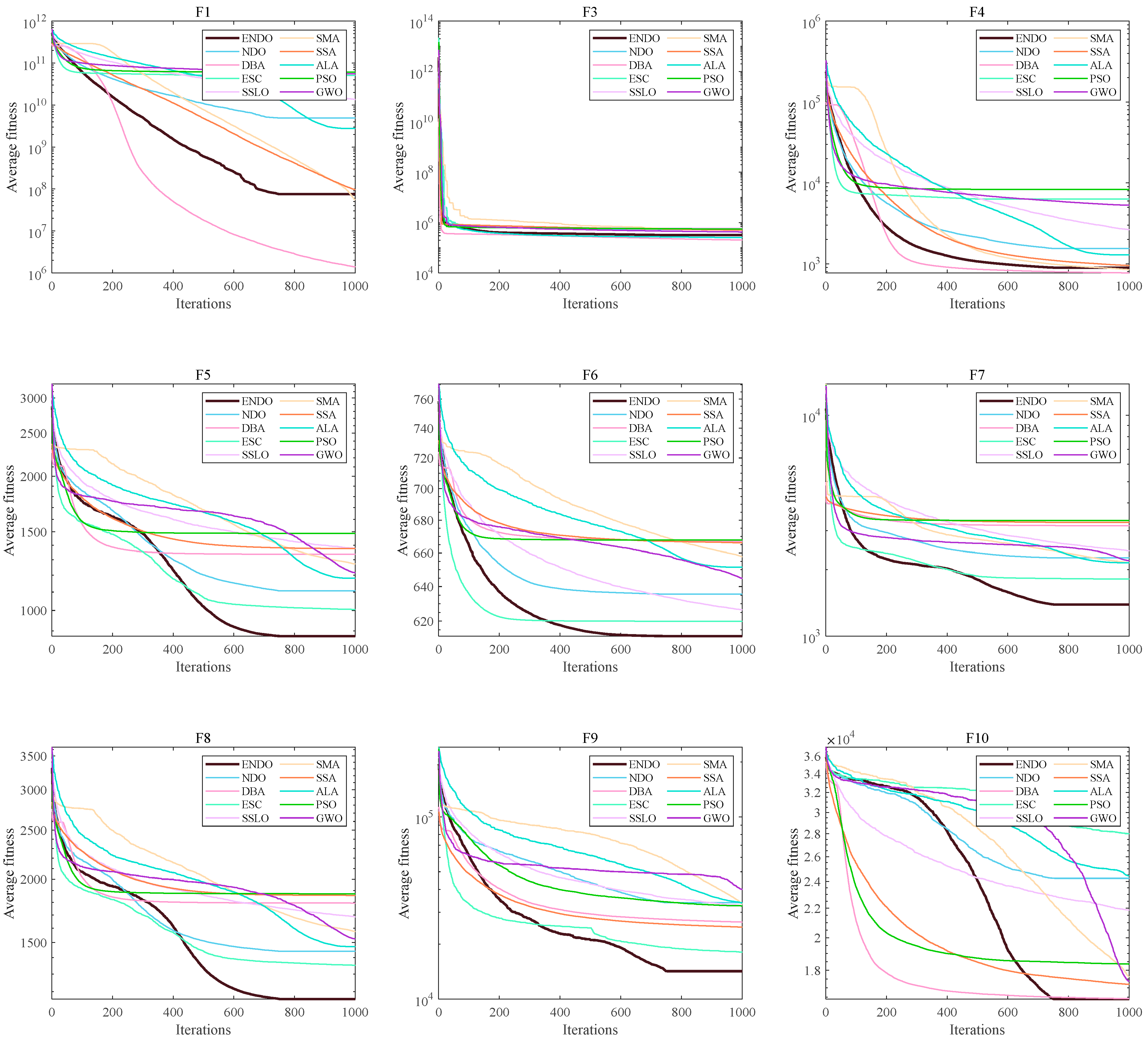
Figure 2 presents the mean convergence curves for F₁ and F₃–F₁₀. On F₁, F₃, and F₄, ENDO converges steadily, although DBA attains a lower final fitness.

For F₅–F₉, ENDO shows a more sustained decrease during the middle and later stages. Several comparison algorithms improve rapidly at the beginning but stagnate earlier, whereas ENDO continues to refine the solution and achieves the best final fitness on these functions. On F₆, ESC converges faster initially, but ENDO obtains the lower terminal value.

On F₁₀, ENDO improves slowly in the early stage and declines sharply after approximately 350 iterations. Although DBA reaches a competitive value earlier, ENDO eventually attains a comparable final result.

Overall, ENDO does not always provide the fastest initial convergence, but it maintains stronger late-stage search capability and is less likely to stagnate prematurely on the multimodal functions.

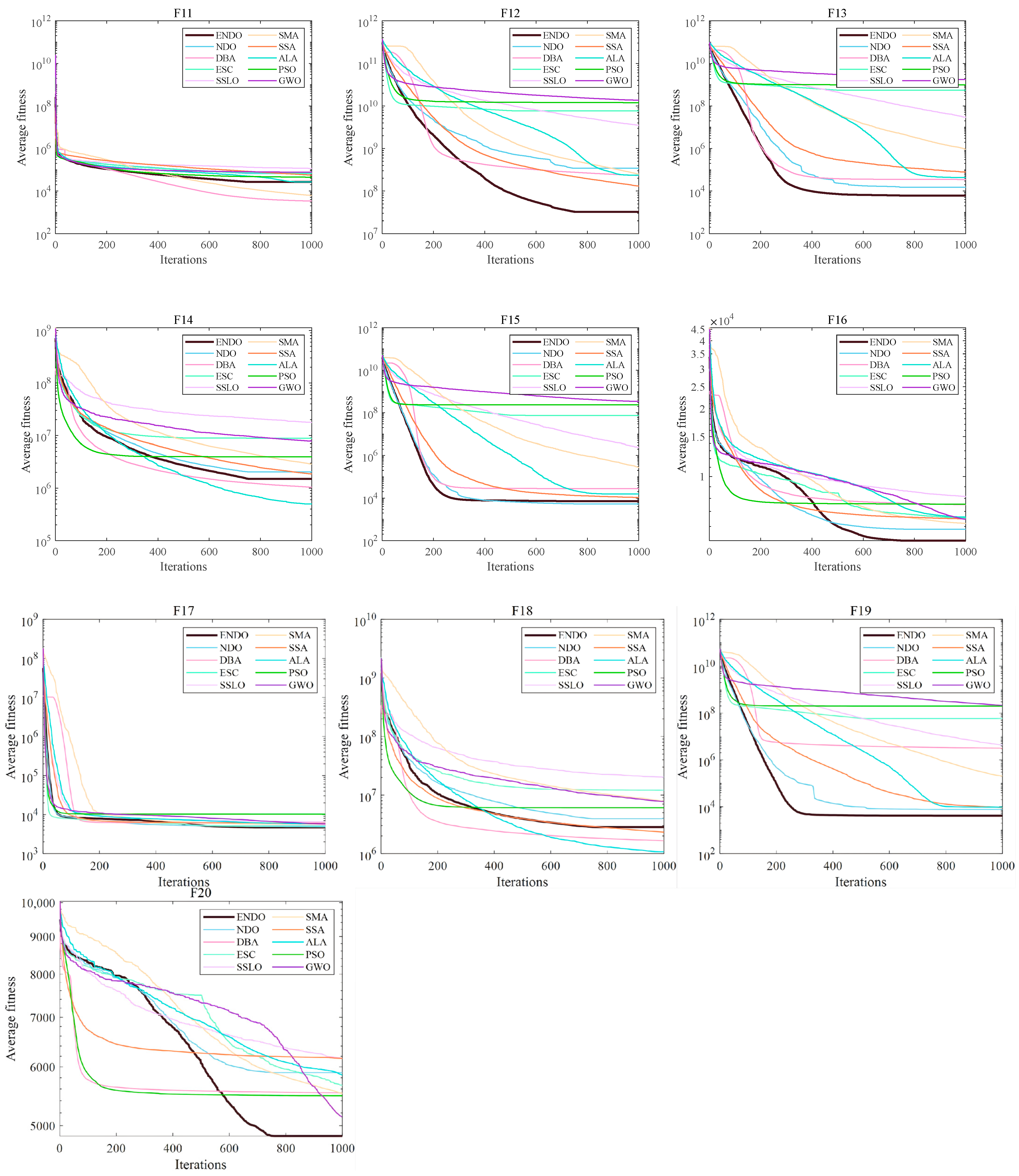
Figure 3 presents the mean convergence curves for F₁₁–F₂₀. ENDO shows clear advantages on F₁₂, F₁₃, F₁₆, F₁₇, F₁₉, and F₂₀. On F₁₂ and F₁₃, it continues to reduce the fitness after most competitors begin to stagnate and reaches the lowest final value. A similar pattern is observed on F₁₆ and F₂₀, where the main improvement occurs during the middle and later stages. On F₁₉, ENDO converges rapidly and stabilizes at the best fitness level.

ENDO shows slightly inferior performance on several functions, including F₁₁, F₁₄, F₁₅, and F₁₈. Specifically, DBA achieves the best result on F₁₁, while ALA performs better on F₁₄ and F₁₈. For F₁₅, ENDO exhibits faster convergence in the early stage, whereas NDO obtains a slightly better final solution. These differences are mainly related to the exploration–exploitation balance of ENDO, which is further analyzed through the population dynamics in Section 3.2.8.

Overall, the curves indicate that ENDO maintains effective search activity on most hybrid functions and often benefits from continued improvement beyond the early iterations. Its advantage is therefore more evident in late-stage refinement than in uniformly faster initial convergence.

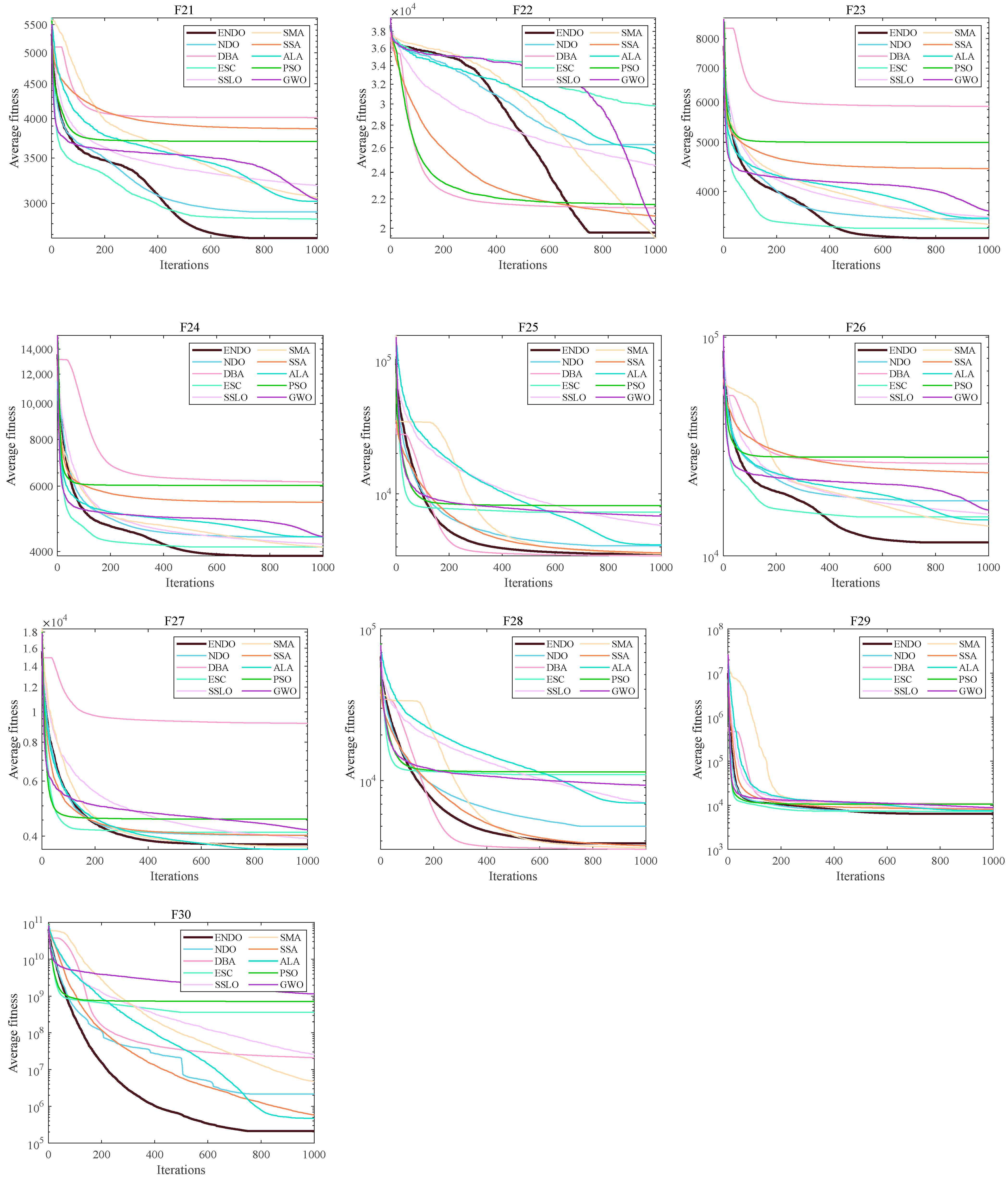
Figure 4 presents the mean convergence curves for F₂₁–F₃₀. ENDO achieves the lowest final fitness on F₂₁, F₂₃, F₂₄, F₂₆, F₂₉, and F₃₀. On F₂₁, F₂₃, F₂₄, and F₂₆, its initial convergence is not always the fastest, but the continued improvement during the middle and later stages leads to better final solutions. ENDO also converges rapidly on F₂₉ and maintains the lowest fitness thereafter. The advantage is particularly evident on F₃₀, where ENDO continues to improve after most comparison algorithms have slowed or stagnated.

On F₂₂, ENDO remains competitive and reaches a final fitness close to the best result. For F₂₅, DBA and SMA attain slightly lower final fitness values than ENDO, while ALA and SMA perform better on F₂₇. On F₂₈, DBA converges faster and achieves the lowest terminal fitness. Overall, ENDO shows strong late-stage refinement on most composition functions, and its convergence behavior is consistent with the statistical results reported in Table 4.

3.2.3. Stability Analysis

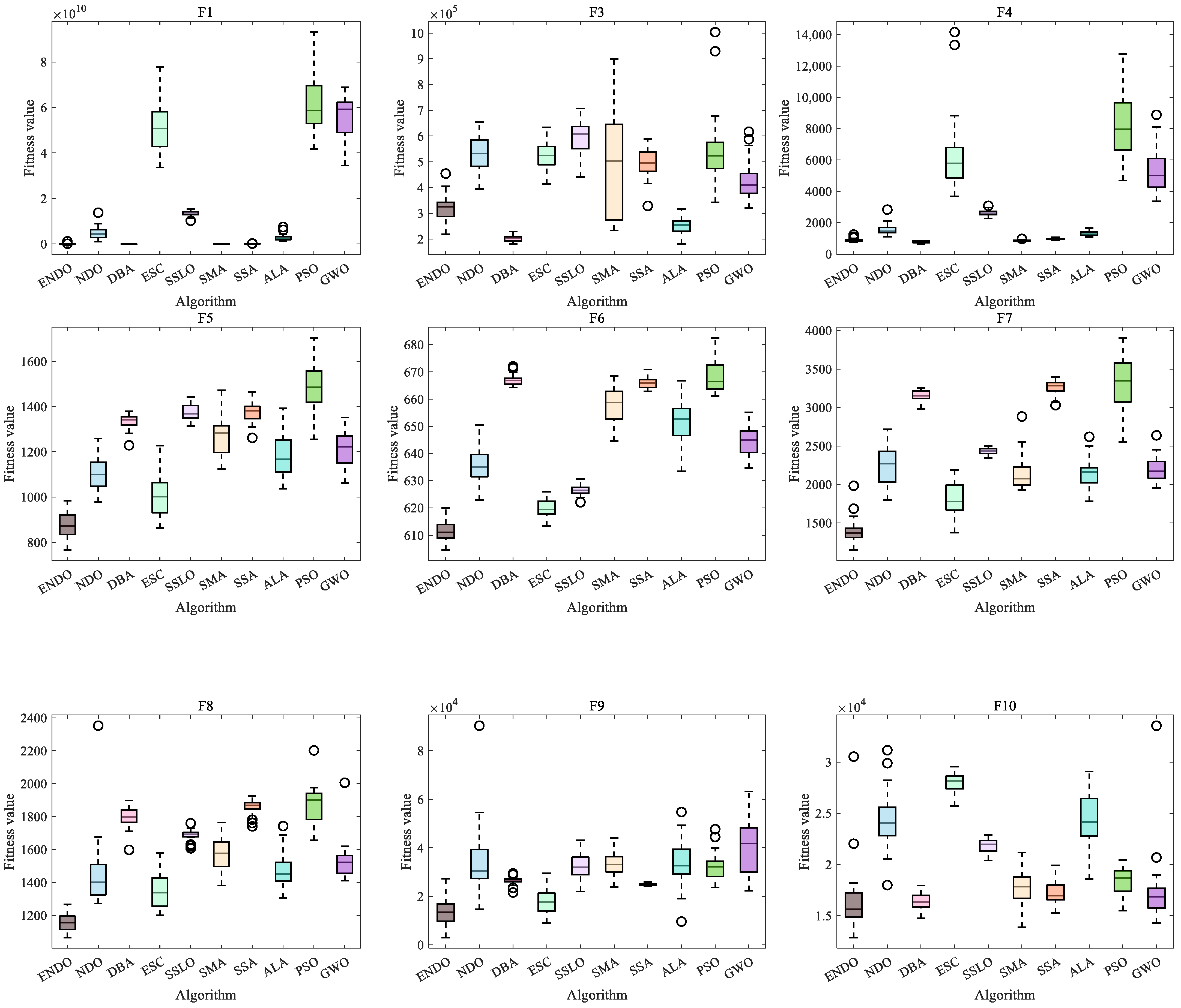
Figure 5 shows the boxplots of the final fitness values for F₁ and F₃–F₁₀ over 30 independent runs. ENDO exhibits relatively compact distributions on most functions. On F₅–F₉, it has the lowest median together with narrow interquartile ranges, indicating that its advantage is maintained across repeated runs rather than being caused by a few favorable results. On F₄, the distribution of ENDO is also concentrated near the best-performing DBA.

For F₁ and F₃, DBA gives lower central fitness values, while ENDO still shows less dispersion than several comparison algorithms. On F₁₀, ENDO obtains the lowest median, although several upper outliers indicate greater variability than DBA. Overall, the boxplots are consistent with the numerical results and show that ENDO provides stable performance on most multimodal functions.

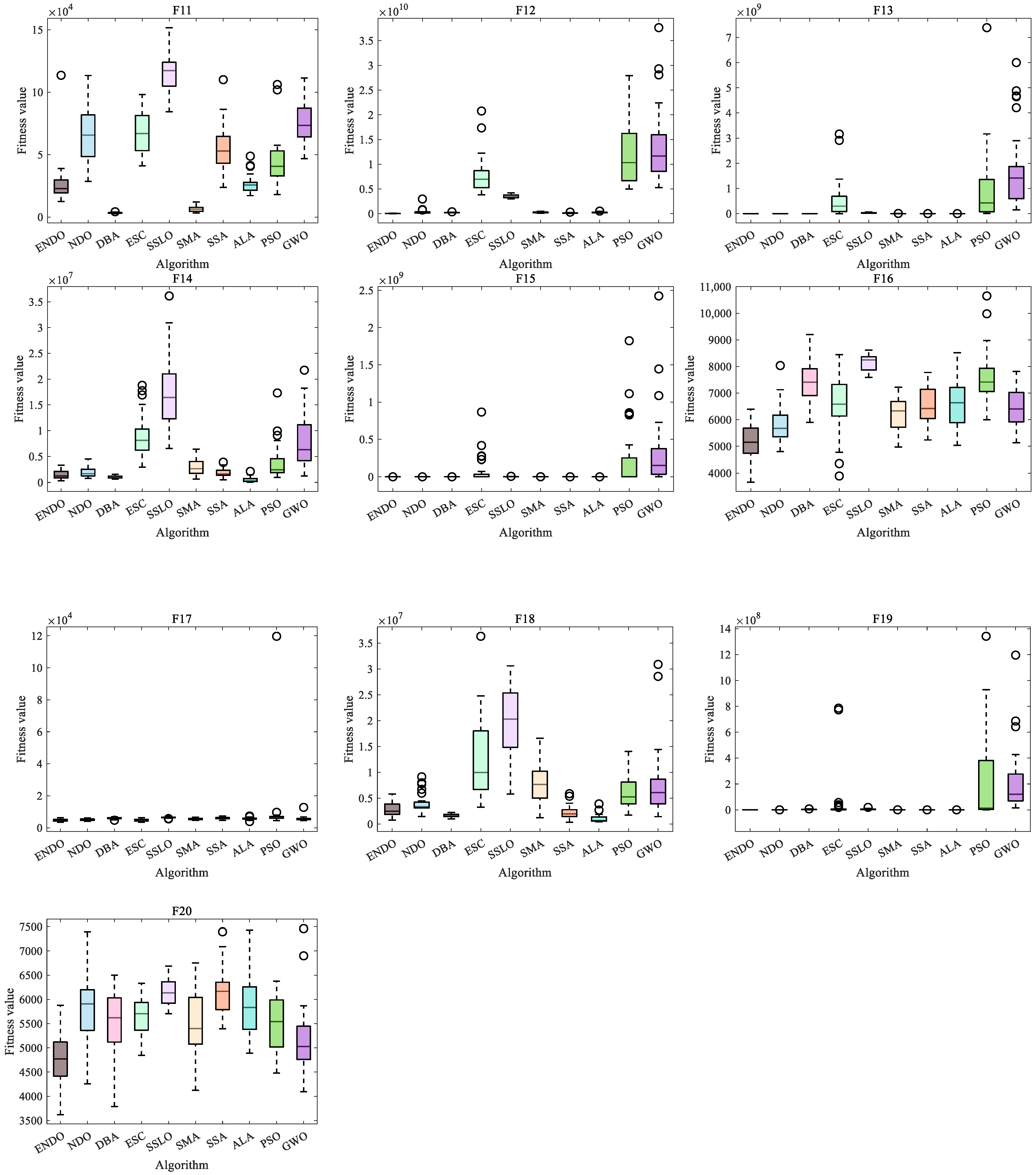
Figure 6 presents the boxplots for F₁₁–F₂₀. On F₁₁, DBA achieves the lowest median and the narrowest distribution, while ENDO remains relatively concentrated compared with most of the other algorithms. For F₁₂ and F₁₃, the ENDO results are tightly clustered near the lowest fitness level, indicating limited variation across the 30 runs.

On F₁₄, ALA and DBA attain lower median fitness values than ENDO. For F₁₅, several algorithms produce similarly low values, whereas ESC, PSO, and GWO show wider distributions and more outliers. ENDO performs more favorably on F₁₆, where it has the lowest median and a compact interquartile range. On F₁₇, its distribution is also narrow and remains within the best-performing group.

For F₁₈, ALA, DBA, and SSA obtain lower median fitness values than ENDO, with ALA showing the most concentrated distribution. On F₁₉, ENDO is tightly clustered near the lowest fitness level and exhibits markedly less variation than ESC, PSO, and GWO. For F₂₀, ENDO attains the lowest median, although its distribution is wider than those observed on F₁₂, F₁₃, F₁₆, F₁₇, and F₁₉.

Overall, ENDO provides low median fitness values with small or moderate dispersion on most hybrid functions. Its stability is particularly evident on F₁₂, F₁₃, F₁₆, F₁₇, and F₁₉, while weaker performance is observed on F₁₁, F₁₄, and F₁₈.

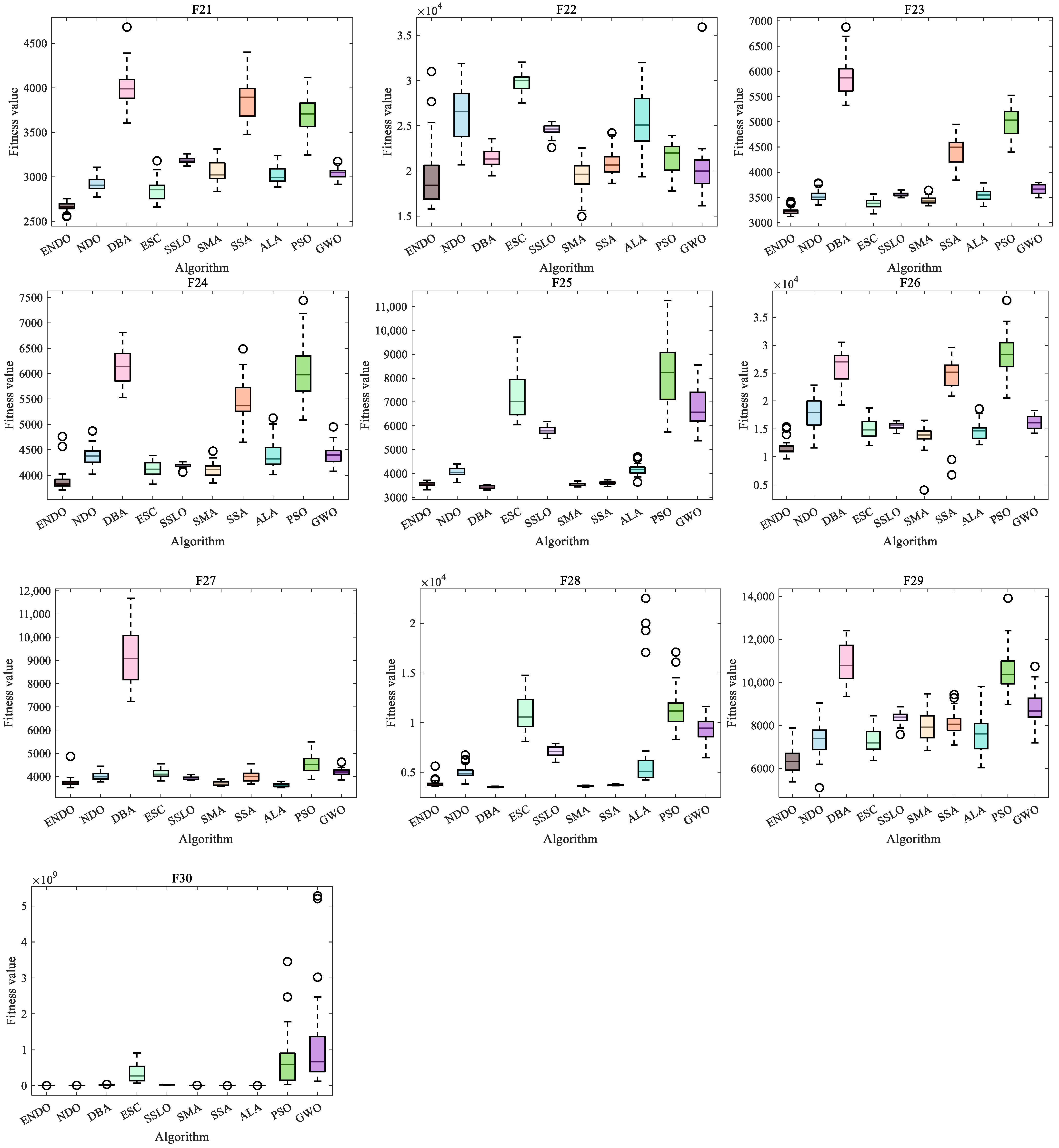
Figure 7 presents the boxplots for F₂₁–F₃₀. ENDO shows the lowest median with a compact interquartile range on F₂₁, F₂₃, F₂₄, and F₂₆. A similar advantage is observed on F₂₉, although its distribution is slightly wider. These results indicate that the favorable mean values reported in Table 4 are generally supported by consistent outcomes across repeated runs.

On F₂₂, SMA achieves the lowest median, followed by ENDO. The ENDO distribution remains relatively compact, although several outliers are observed. For F₂₅, DBA provides the lowest and most concentrated distribution, while ENDO remains close to SMA and SSA. On F₂₇, ALA and SMA obtain lower median values than ENDO. For F₂₈, DBA, SMA, and SSA achieve lower medians, whereas ENDO still maintains a narrow distribution.

On F₃₀, ENDO and several competing algorithms produce tightly clustered results near the lowest fitness level, while PSO and GWO exhibit substantially larger dispersion and several poor runs. Overall, ENDO combines low median fitness with small or moderate variability on most composition functions, with weaker relative performance mainly observed on F₂₅, F₂₇, and F₂₈.

3.2.4. Statistical Significance and Ranking Analysis

To assess pairwise statistical differences, the Wilcoxon rank-sum test was applied to the 30 independent results obtained by ENDO and each comparison algorithm at α = 0.05.

Table 5. Category-wise Wilcoxon rank-sum results and Holm-corrected post hoc comparisons on the 100-dimensional CEC2017 benchmark.

Comparison	Unimodal (2) (+/=/−)	Multimodal (7) (+/=/−)	Hybrid (10) (+/=/−)	Composition (10) (+/=/−)	Overall (29) (+/=/−)	Holm-Adjusted p
ENDO vs. NDO	2/0/0	7/0/0	8/1/1	10/0/0	27/1/1	1.65 × 10−4
ENDO vs. DBA	0/0/2	5/1/1	7/1/2	8/0/2	20/2/7	3.17 × 10−5
ENDO vs. ESC	2/0/0	7/0/0	9/1/0	10/0/0	28/1/0	1.17 × 10−6
ENDO vs. SSLO	2/0/0	7/0/0	10/0/0	10/0/0	29/0/0	7.87 × 10−11
ENDO vs. SMA	1/0/1	6/0/1	9/0/1	6/3/1	22/3/4	2.08 × 10−3
ENDO vs. SSA	2/0/0	7/0/0	8/2/0	9/1/0	26/3/0	1.41 × 10−5
ENDO vs. ALA	1/0/1	7/0/0	7/1/2	9/0/1	24/1/4	7.52 × 10−4
ENDO vs. PSO	2/0/0	7/0/0	10/0/0	10/0/0	29/0/0	5.18 × 10−16
ENDO vs. GWO	2/0/0	7/0/0	9/1/0	9/1/0	27/2/0	9.63 × 10−10

Note: “+/=/−” denotes the number of functions on which ENDO performs significantly better than, shows no significant difference from, or performs significantly worse than the corresponding algorithm according to the Wilcoxon rank-sum test at α = 0.05. Holm-adjusted p-values are obtained from post hoc comparisons following the Friedman test, with ENDO as the control algorithm.

summarizes the resulting win/tie/loss counts together with the Holm-adjusted p-values from the post hoc analysis.

As shown in Table 5, ENDO records 27 wins, one tie, and one loss against NDO, showing a clear statistical advantage on most test functions. Because ENDO involves additional function evaluations, the effect of the evaluation budget is examined separately in Section 3.2.6. ENDO also significantly outperforms SSLO and PSO on all 29 functions. The results against ESC, SSA, and GWO are 28/1/0, 26/3/0, and 27/2/0, respectively, with no significant losses.

Against the stronger competitors DBA, SMA, and ALA, ENDO obtains 20/2/7, 22/3/4, and 24/1/4, respectively. Although several losses are observed, the number of significant wins remains substantially higher. The category-wise results also show that ENDO is less competitive than DBA on the two unimodal functions, whereas it records 5, 7, and 8 significant wins on the multimodal, hybrid, and composition functions, respectively. Similar trends are observed against SMA and ALA, indicating that the advantage of ENDO is more pronounced on complex search landscapes.

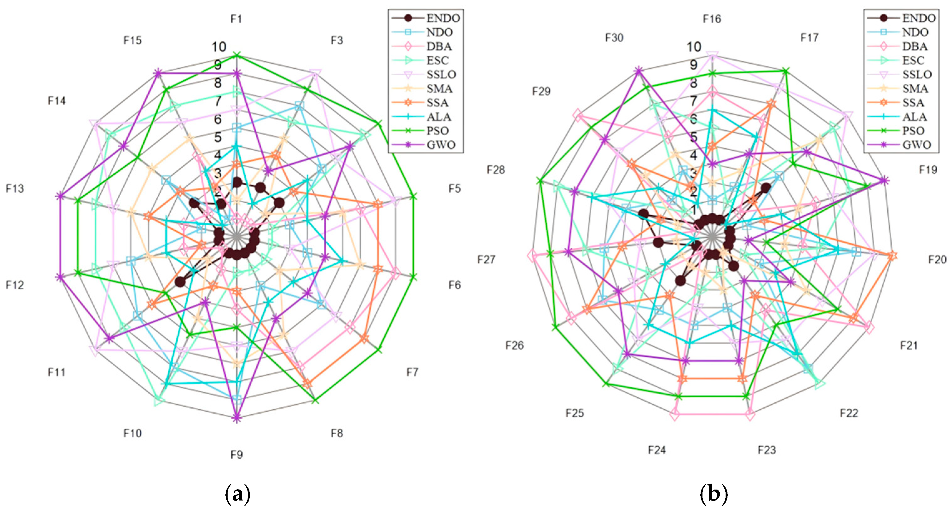
Figure 8 presents the function-wise ranking distributions. A lower rank, represented by a position closer to the center of the radar chart, indicates better performance. ENDO remains in the inner region on most functions and ranks among the top three on 26 of the 29 functions. Its lowest position is fourth, showing that its performance does not deteriorate markedly on any particular function.

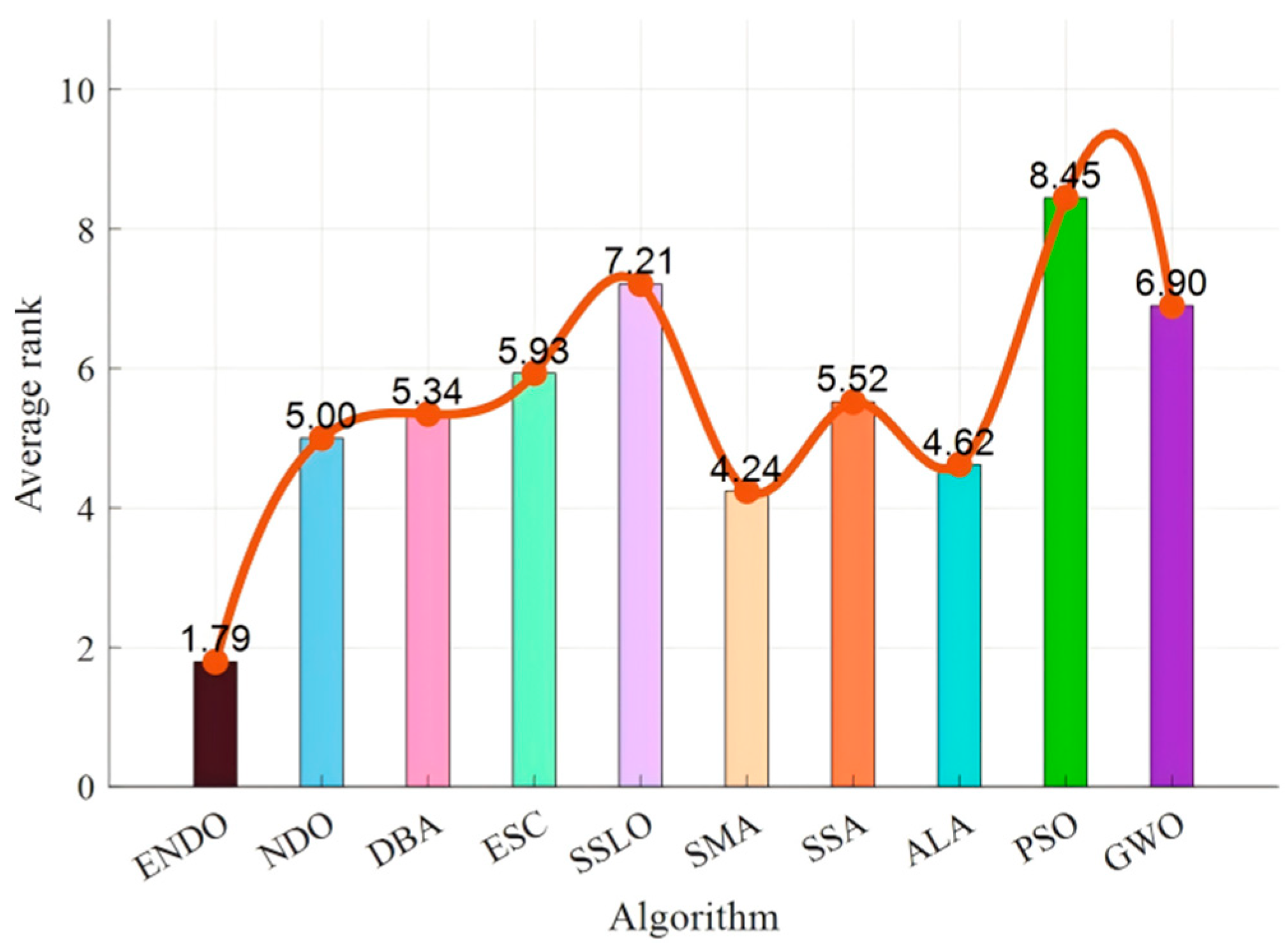
The average rankings are shown in Figure 9. ENDO achieves the best average rank of 1.79, followed by SMA and ALA with average ranks of 4.24 and 4.62, respectively. The corresponding ranks for NDO, DBA, SSA, ESC, GWO, SSLO, and PSO are 5.00, 5.34, 5.52, 5.93, 6.90, 7.21, and 8.45. The difference of 2.45 between ENDO and the second-ranked algorithm indicates that its advantage is distributed across the benchmark rather than being determined by a small number of functions.

An omnibus Friedman test across the ten algorithms and 29 functions showed a significant overall difference, with ${\chi }^2(9)=95.27$ and $p=1.42\times {10}^{-16}$. Holm-corrected post hoc comparisons were then performed with ENDO as the control algorithm. All nine comparisons remained significant after correction, with adjusted p-values ranging from 5.18 × 10⁻¹⁶ to 2.08 × 10⁻³.

Overall, the Wilcoxon, Friedman–Holm, and ranking results are consistent with the numerical results in Table 2, Table 3 and Table 4. ENDO achieves the best average rank of 1.79, and all nine Holm-corrected comparisons are significant. Against NDO, the Wilcoxon result is 27/1/1, with F14 being the only nonsignificant case and F15 favoring NDO.

3.2.5. Comparison with Advanced Optimizers

To assess ENDO against stronger baselines, six advanced optimizers, namely CMA-ES, SHADE, L-SHADE, LSHADE-SPACMA, EBOwithCMAR, and jSO, were further compared at 100 dimensions. ENDO and NDO were included as references, and all methods followed the unified experimental protocol described in Section 3.1. The results are summarized in

Table 6. Overall comparison of ENDO with advanced optimizers on the 100-dimensional CEC2017 benchmark.

Algorithm	Average Rank	ENDO vs. Algorithm (+/=/−)	Holm-Adjusted p
CMA-ES	2.90	6/2/21	1.000
SHADE	3.07	12/5/12	1.000
ENDO	3.52	—	—
EBOwithCMAR	3.86	14/3/12	1.000
jSO	5.24	21/2/6	2.94 × 10−2
LSHADE-SPACMA	5.45	24/2/3	1.34 × 10−2
L-SHADE	5.55	18/3/8	9.38 × 10−3
NDO	6.41	27/1/1	4.69 × 10−5

Note: “+/=/−” denotes the number of functions on which ENDO performs significantly better than, shows no significant difference from, or performs significantly worse than the corresponding algorithm according to the two-sided Wilcoxon rank-sum test at α = 0.05. Holm-adjusted p-values are obtained from post hoc comparisons following the Friedman test, with ENDO as the control algorithm.

.

CMA-ES achieved the lowest average rank of 2.90, followed by SHADE with 3.07. ENDO ranked third with an average rank of 3.52, ahead of EBOwithCMAR, jSO, LSHADE-SPACMA, L-SHADE, and NDO. The Wilcoxon results show that ENDO obtained more significant wins than losses against these five algorithms. In contrast, CMA-ES was stronger on most functions, while ENDO and SHADE showed a balanced 12/5/12 outcome.

The Friedman test indicated significant overall differences among the eight algorithms (${\chi }^2(7)=59.01, p=2.38\times {10}^{-10}$). After Holm correction, significant differences were observed between ENDO and NDO, L-SHADE, LSHADE-SPACMA, and jSO, whereas the differences with CMA-ES, SHADE, and EBOwithCMAR were not significant. These results show that ENDO remains competitive against stronger optimizers, although it does not consistently outperform all of them.

Because the compared methods were evaluated under the unified N/T protocol rather than their original competition-specific configurations, the rankings reported here are specific to the present experimental settings.

3.2.6. Function-Evaluation Budget Fairness Analysis

The primary benchmark experiments used the same population size and iteration limit, but NDO and ENDO require different numbers of objective-function evaluations (FEs). In addition to the basic NDO update, ENDO evaluates candidates generated by the inferior-individual mutation and opposition-based search and re-evaluates the population at the end of each iteration. An FE-matched experiment was therefore conducted to examine whether the performance improvement of ENDO was mainly due to its larger evaluation budget.

For NDO, initialization requires N evaluations, and each iteration requires 3N evaluations. ENDO requires additional evaluations for inferior-individual mutation, opposition-based search, and population re-evaluation. The FE budgets of NDO, ENDO, and the FE-matched NDO variant (NDO-FE) are calculated as shown in Equation (10):

$$\begin{array}{l}{\mathrm{FE}}_{\mathrm{NDO}}=N+3NT,\\ {\mathrm{FE}}_{\mathrm{ENDO}}=N+T\left(6N+N_{\mathrm{poor}}\right),\\ {\mathrm{FE}}_{\mathrm{NDO}\text{-}\mathrm{FE}}=N+3N{T}_{\mathrm{FE}}\end{array}$$

(10)

where N is the population size, T is the iteration limit of the original experiment, $T_{\mathrm{FE}}$ is the iteration limit of NDO-FE, and $N_{\mathrm{poor}}=N-⌈0.7N⌉+1$ is the number of inferior individuals selected for mutation according to Section 2.2.2. For N = 30, $N_{\mathrm{poor}}=10$.

With N = 30 and T = 1000, Equation (10) gives 90,030 FEs for NDO and 190,030 FEs for ENDO. For NDO-FE, the original NDO search operators were retained, and only the iteration limit was increased to $T_{\mathrm{FE}}=2111$, resulting in 190,020 FEs. Thus, ENDO and NDO-FE differ by only 10 evaluations, corresponding to approximately 0.0053% of the ENDO evaluation budget.

The FE budgets and statistical results are summarized in

Table 7. FE budgets and statistical comparison of ENDO, NDO, and NDO-FE on the 100-dimensional CEC2017 benchmark.

Algorithm	Iterations	FEs	Average Rank	ENDO vs. Algorithm (+/=/−)
ENDO	1000	190,030	1.07	—
NDO	1000	90,030	2.41	27/1/1
NDO-FE	2111	190,020	2.52	25/3/1

Note: “+/=/−” denotes the number of functions on which ENDO performs significantly better than, shows no significant difference from, or performs significantly worse than the corresponding algorithm according to the Wilcoxon rank-sum test at α = 0.05. The average ranks are calculated among the three algorithms in this comparison.

.

As shown in Table 7, ENDO achieved the best average rank of 1.07, compared with 2.41 for NDO and 2.52 for NDO-FE. Although NDO-FE used nearly the same FE budget as ENDO, ENDO obtained a lower mean fitness value on 28 of the 29 functions. The Wilcoxon rank-sum test yielded a 25/3/1 win/tie/loss result for ENDO against NDO-FE. No significant difference was observed on F14, F17, and F19, whereas NDO-FE was significantly better only on F15.

Increasing the evaluation budget of NDO from 90,030 to 190,020 FEs did not yield a corresponding performance improvement. From the perspective of NDO-FE, the Wilcoxon comparison with NDO yielded 0/26/3 wins/ties/losses, indicating that NDO-FE did not significantly outperform NDO on any of the 29 functions. Thus, increasing the evaluation budget alone was insufficient to reproduce the performance achieved by ENDO.

3.2.7. Ablation Study

To examine the contribution of ADM, IGM, and DOBL, a complete ablation study was conducted on the 100-dimensional CEC2017 benchmark. The comparison included the original NDO, three single-mechanism variants, three dual-mechanism variants, and the complete ENDO. All configurations were evaluated on F1 and F3–F30 with N = 30, T = 1000, and 30 independent runs. The remaining experimental settings were unchanged.

Table 8. Ablation results of ADM, IGM, and DOBL on the 100-dimensional CEC2017 benchmark.

Algorithm	ADM	IGM	DOBL	FEs	Average Rank	First	Top 3	ENDO vs. Algorithm (+/=/−)
NDO	—	—	—	90,030	6.48	0	0	27/1/1
NDO-ADM	✔	—	—	90,030	5.34	2	8	23/4/2
NDO-IGM	—	✔	—	100,030	5.45	1	5	21/7/1
NDO-DOBL	—	—	✔	180,030	5.62	0	0	25/4/0
NDO-ADM-IGM	✔	✔	—	100,030	2.90	3	18	13/16/0
NDO-ADM-DOBL	✔	—	✔	180,030	5.03	0	12	20/8/1
NDO-IGM-DOBL	—	✔	✔	190,030	3.38	5	18	17/11/1
ENDO	✔	✔	✔	190,030	1.79	18	26	—

Note: Average Rank, First, and Top 3 are calculated among the eight ablation configurations. “+/=/−” denotes the number of functions on which ENDO performs significantly better than, shows no significant difference from, or performs significantly worse than the corresponding configuration according to the Wilcoxon rank-sum test at α = 0.05. ADM denotes adaptive dimension mask; IGM denotes inferior-individual greedy mutation; DOBL denotes dynamic-boundary opposition-based learning; and FEs denote function evaluations.

summarizes the mechanism composition, function-evaluation budget, average rank, number of first-place and top-three results, and the Wilcoxon comparisons between ENDO and the other configurations.

As shown in Table 8, ENDO achieved the best average rank of 1.79, ranking first on 18 functions and within the top three on 26 functions. Among the dual-mechanism variants, NDO-ADM-IGM and NDO-IGM-DOBL obtained average ranks of 2.90 and 3.38, respectively. ENDO yielded win/tie/loss results of 13/16/0 against NDO-ADM-IGM and 17/11/1 against NDO-IGM-DOBL. NDO-IGM-DOBL and ENDO used the same budget of 190,030 FEs. Under this matched budget, ENDO retained a lower average rank and significantly outperformed NDO-IGM-DOBL on 17 functions, indicating an additional contribution from ADM.

The single-mechanism variants obtained average ranks of 5.34 for NDO-ADM, 5.45 for NDO-IGM, and 5.62 for NDO-DOBL, compared with 6.48 for NDO. Their improvements were therefore limited and varied across functions. The dual-mechanism variants generally achieved better rankings, particularly NDO-ADM-IGM and NDO-IGM-DOBL. The complete ENDO achieved the best overall result, suggesting that ADM, IGM, and DOBL provide complementary contributions to the search process.

3.2.8. Population Diversity and Step-Size Dynamics Analysis

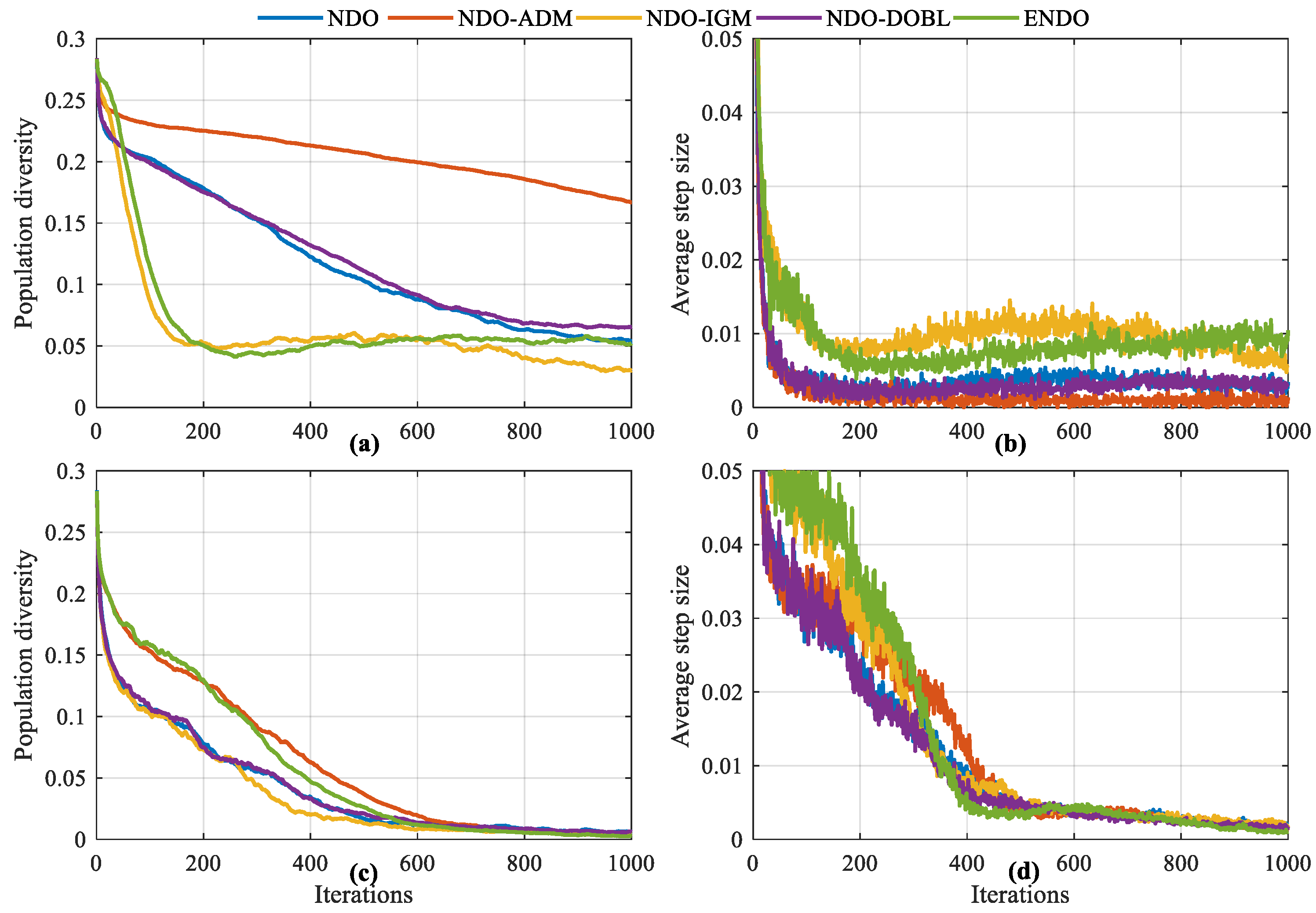
To investigate the influence of different mechanisms on the search behavior of ENDO, the variations of population diversity and average step size were analyzed during the optimization process. Figure 10 presents the dynamic changes of different algorithm variants on two representative benchmark functions (F11 and F15).

As shown in Figure 10a, the population diversity of all algorithms gradually decreases with iterations, indicating a transition from exploration to exploitation. NDO-ADM maintains a higher diversity level during the search process, demonstrating that the adaptive mechanism can enhance population diversity. In contrast, NDO-IGM exhibits a faster diversity reduction, which indicates stronger exploitation behavior. NDO-DOBL maintains a moderate diversity level because the opposite learning mechanism introduces additional candidate solutions and enlarges the search space, which helps improve the ability to escape local optima. ENDO maintains a moderate diversity level, suggesting that the combination of multiple mechanisms achieves a balance between exploration and exploitation.

Figure 10b illustrates the changes in average step size on F11. Compared with the original NDO, ENDO maintains a relatively larger step size in the middle and later stages, providing additional exploration ability. This property helps reduce premature convergence but may also weaken local refinement on some specific landscapes, which explains why ENDO does not always achieve the best final solution on functions dominated by strong exploitation requirements.

For F15, Figure 10c,d show similar dynamic characteristics. ENDO preserves a larger search range in the early stage and gradually reduces the step size as the iteration proceeds, enabling rapid exploration and stable exploitation. However, algorithms with stronger exploitation ability may obtain better final solutions on certain functions due to more effective local search.

Overall, the dynamic analysis indicates that the proposed mechanisms regulate population diversity and search step size, enabling ENDO to achieve a better balance between exploration and exploitation.

3.2.9. Parameter Sensitivity Analysis

To assess the influence of the main control parameters on ENDO, a sensitivity analysis was performed on the 100-dimensional CEC2017 benchmark. Five factors were examined: the endpoints of the adaptive dimension-mask threshold, fixed mask thresholds, the inferior-individual cutoff q, the mutation probability $p_{\mathrm{m}}$, and the execution interval of DOBL. One factor was varied at a time, with the remaining settings unchanged. All experiments used N = 30, T = 1000, and 30 independent runs. The ENDO results from the main benchmark experiment were retained as the baseline to maintain consistency with the reported results. For inferior-individual mutation, q defines the starting rank $⌈qN⌉$; thus, q = 0.7 selects individuals ranked from $⌈0.7N⌉$ to N. The results are summarized in

Table 9. Parameter sensitivity analysis of ENDO on the 100-dimensional CEC2017 benchmark.

Parameter	Setting	Average Rank	ENDO vs. Variant (+/=/−)
ADM endpoints	0.1–0.5	3.34	6/19/4
	0.2–0.6	2.55	1/22/6
	0.3–0.7 (baseline)	2.41	—
	0.4–0.8	3.17	6/23/0
	0.5–0.9	3.52	14/13/2
Mask threshold	Fixed 0.3	2.34	6/21/2
	Fixed 0.5	2.59	10/19/0
	Fixed 0.7	3.28	17/10/2
	Adaptive 0.3–0.7 (baseline)	1.79	—
Inferior cutoff q	0.5	2.83	2/24/3
	0.6	2.76	3/24/2
	0.7 (baseline)	2.59	—
	0.8	3.03	7/21/1
	0.9	3.79	17/9/3
Mutation probability $p_{\mathrm{m}}$	0.3	3.90	11/16/2
	0.4	3.03	6/21/2
	0.5 (baseline)	2.62	—
	0.6	2.72	2/24/3
	0.7	2.72	0/26/3
DOBL interval	1 (baseline)	1.69	—
	2	2.24	2/26/1
	5	2.93	7/22/0
	10	3.14	9/20/0

Note: Average ranks are calculated separately within each parameter group. “+/=/−” denotes the number of functions on which the baseline ENDO performs significantly better than, shows no significant difference from, or performs significantly worse than the corresponding variant according to the Wilcoxon rank-sum test at α = 0.05.

.

As shown in Table 9, the baseline ADM endpoints of 0.3→0.7 achieved the lowest average rank of 2.41 among the five endpoint settings. The 0.2→0.6 setting produced a similar rank of 2.55, while the ranks for 0.1→0.5, 0.4→0.8, and 0.5→0.9 were 3.34, 3.17, and 3.52, respectively. The close results obtained with 0.3→0.7 and 0.2→0.6 suggest limited sensitivity to moderate changes in the endpoint values. A more distinct difference was observed when the adaptive schedule was replaced by a fixed threshold. The adaptive 0.3→0.7 schedule obtained an average rank of 1.79, compared with 2.34, 2.59, and 3.28 for fixed thresholds of 0.3, 0.5, and 0.7, respectively. The corresponding Wilcoxon results were 6/21/2, 10/19/0, and 17/10/2. Under the tested settings, the adaptive schedule therefore provided better overall performance than the three fixed-threshold alternatives.

For the inferior-individual cutoff, q = 0.7 achieved the lowest average rank of 2.59. The ranks obtained with q = 0.5 and q = 0.6 were 2.83 and 2.76, respectively, whereas increasing q to 0.8 and 0.9 resulted in ranks of 3.03 and 3.79, respectively. A smaller q applies mutation to a larger portion of the lower-ranked population, while a larger q limits mutation to fewer individuals. Among the tested values, q = 0.7 gave the best overall ranking without extending the mutation operation to an excessively large portion of the population.

The mutation probability showed weaker sensitivity within the middle-to-high range. The baseline setting $p_{\mathrm{m}}=0.5$ obtained the lowest average rank of 2.62, while both $p_{\mathrm{m}}=0.6$ and $p_{\mathrm{m}}=0.7$ yielded 2.72. The average ranks increased to 3.03 and 3.90 when $p_{\mathrm{m}}$ was reduced to 0.4 and 0.3, respectively. The relatively small differences among 0.5, 0.6, and 0.7 suggest that the mutation stage is not highly sensitive to the probability setting within this range.

The DOBL execution interval produced a clearer trend. Applying DOBL at every iteration yielded the lowest average rank of 1.69. Increasing the interval to 2, 5, and 10 iterations increased the average rank to 2.24, 2.93, and 3.14, respectively. In addition, the interval-5 and interval-10 variants did not significantly outperform the baseline on any of the 29 functions. Less frequent application of DOBL was therefore associated with poorer overall performance under the present implementation. Since changing the DOBL interval also changes the number of opposition-based objective-function evaluations, this comparison reflects both the search frequency and the associated evaluation effort.

Overall, the baseline setting achieved the lowest average rank in each of the five parameter groups. Several neighboring settings, particularly the ADM endpoints of 0.2→0.6 and mutation probabilities of 0.6–0.7, remained close to the baseline. Larger deviations generally resulted in lower overall rankings. This suggests that the adopted parameter values are effective across the benchmark set while retaining a degree of tolerance to moderate parameter variation.

3.3. Cross-Dimensional Scalability Analysis

The preceding analysis focused on the 100-dimensional case. To assess the sensitivity of ENDO to problem size, the results obtained at 10, 30, and 50 dimensions are compared with those at 100 dimensions, with emphasis on ranking performance and cross-dimensional trends.

3.3.1. Overall Results Across Different Dimensions

Table 10. Ranking performance of ENDO across different dimensions on the CEC2017 benchmark.

Dimension	First	Second	Third	Top Three	Worst Rank	Average Rank	ENDO vs. NDO
10D	14	9	4	27	4	1.79	28/0/1
30D	16	10	0	26	4	1.66	28/0/1
50D	20	7	2	29	3	1.38	29/0/0
100D	18	2	6	26	4	1.79	28/0/1

summarizes the ranking performance of ENDO at 10, 30, 50, and 100 dimensions. The columns First, Second, and Third indicate the number of functions on which ENDO obtains the corresponding rank, while Top three gives the total number of functions ranked within the three best algorithms. The last column reports the number of functions on which ENDO achieves a lower, equal, or higher mean fitness value than NDO.

ENDO maintains a low average rank across all four dimensions, ranging from 1.38 to 1.79. At 10 dimensions, it ranks among the top three on 27 functions, including 14 first-place results. At 30 dimensions, the number of first-place results increases to 16, and the average rank improves from 1.79 to 1.66.

The best overall result is obtained at 50 dimensions, where ENDO ranks first on 20 functions and remains among the top three on all 29 functions, giving an average rank of 1.38. At 100 dimensions, ENDO still ranks first on 18 functions and among the top three on 26 functions. Its average rank remains 1.79, indicating that the increase in dimensionality does not cause a marked decline in overall performance.

Compared with NDO, ENDO achieves lower mean fitness values on 28 functions at 10, 30, and 100 dimensions, and on all 29 functions at 50 dimensions. This consistent improvement across different problem scales indicates that the proposed strategies enhance the original algorithm without restricting its effectiveness to a specific dimension.

3.3.2. Dimension-Wise Ranking and Robustness

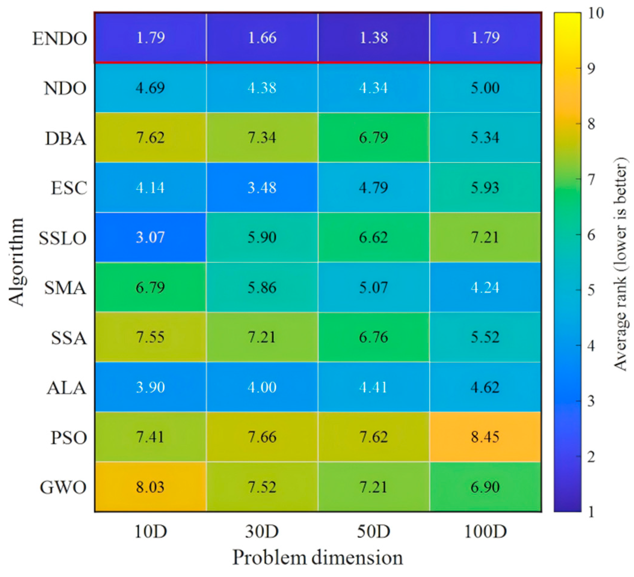
Figure 11 presents the heatmap of the average rankings obtained by the compared algorithms at 10, 30, 50, and 100 dimensions. A lower average rank indicates better overall performance.

ENDO achieves the lowest average rank at every dimension, with values of 1.79, 1.66, 1.38, and 1.79, respectively. The limited variation among these values suggests that its relative performance is not strongly dependent on a particular problem dimension. Its best result occurs at 50 dimensions, while the average rank remains unchanged at 1.79 between the 10- and 100-dimensional cases.

NDO and ALA also show relatively moderate changes across dimensions, although their rankings remain clearly above those of ENDO. The average rank of NDO varies from 4.34 to 5.00, whereas that of ALA ranges from 3.90 to 4.62. ESC performs best at 30 dimensions with an average rank of 3.48, but its ranking increases to 4.79 and 5.93 at 50 and 100 dimensions, respectively, indicating weaker relative performance as dimensionality increases.

SSLO exhibits the clearest dimension-dependent decline. Its average rank changes from 3.07 at 10 dimensions to 5.90, 6.62, and 7.21 at 30, 50, and 100 dimensions, respectively. In contrast, SMA, DBA, and SSA generally improve as the dimension increases. For example, the average rank of SMA decreases from 6.79 at 10 dimensions to 4.24 at 100 dimensions. PSO remains among the lower-ranked algorithms at all dimensions and reaches an average rank of 8.45 at 100 dimensions.

Overall, ENDO combines the lowest average ranking with limited variation across the four problem dimensions. The results in Table 10 and Figure 11 therefore indicate that ENDO retains competitive performance in low-, medium-, and high-dimensional search spaces.

3.4. Discussion

In the primary 100-dimensional CEC2017 comparison, ENDO ranks first on 18 functions and remains among the top three on 26 functions, with an average rank of 1.79. In the additional comparison with six advanced optimizers, ENDO ranks third with an average rank of 3.52, indicating competitive performance against stronger baselines under the unified experimental protocol. The cross-dimensional experiments further show average ranks of 1.79, 1.66, 1.38, and 1.79 at 10, 30, 50, and 100 dimensions, respectively, all lower than those of the primary comparison algorithms. Relative to the original NDO, ENDO obtains lower mean fitness values on 28, 28, 29, and 28 functions at the four dimensions. The improvement is therefore not restricted to a particular problem size.

The advantage of ENDO is more evident on multimodal, hybrid, and composition functions. The adaptive dimension mask adjusts the update pattern of different dimensions during the search. The DE/rand/2-based greedy mutation provides additional search opportunities for inferior individuals, while the dynamic-boundary opposition-based guidance broadens the generation of promising candidates. These mechanisms are consistent with the sustained middle- and late-stage decrease observed in the convergence curves, suggesting that ENDO can mitigate premature stagnation and retain effective local refinement on most complex functions.

ENDO does not obtain the best result on every function. Other algorithms perform better on several unimodal functions and on F11, F18, and F28. This shows that the relative advantage of ENDO still depends on the landscape characteristics of the test problem. Its improvement is more apparent in multimodal, strongly coupled, and structurally complex search spaces, whereas the advantage is less pronounced on some simpler or specially structured functions.

Overall, the improvement achieved by ENDO is mainly reflected in its sustained search capability and adaptability across different dimensions. The 100-dimensional results, statistical tests, and dimension-wise rankings show consistent trends. This suggests that the three strategies strengthen population exploration while preserving effective late-stage exploitation, thereby improving the overall performance of the algorithm on complex optimization problems.

4. Application of ENDO to Thermal–Pumped-Storage Economic Dispatch

To evaluate the applicability of ENDO to high-dimensional engineering optimization problems with multiple constraints, it is applied to the economic dispatch of a thermal–pumped-storage power system. The objective is to coordinate the outputs of thermal units and the operating power of the pumped-storage station over a 24 h scheduling horizon while satisfying power-demand and equipment-operation constraints, thereby minimizing the total operating cost.

4.1. Problem Description

The investigated power system consists of six adjustable thermal generating units, four fixed-output power sources, and one pumped-storage station. The scheduling horizon is 24 h with a time interval of 1 h. The outputs of the four fixed power sources are 150, 200, 300, and 300 MW, respectively, resulting in a constant total output of 950 MW throughout the scheduling horizon. The remaining system demand is jointly supplied by the six thermal units and the pumped-storage station.

The pumped-storage station can operate in either generation or pumping mode during each scheduling period according to the system load, thermal-generation cost, and stored-energy level. When $P_t^{\mathrm{ps}}>0$, the station operates in generation mode and supplies power to the system. When $P_t^{\mathrm{ps}}<0$, it operates in pumping mode and consumes power from the system. Its operating power is bounded within $-300\le P_t^{\mathrm{ps}}\le 300 \mathrm{MW}$.

Each thermal unit contains 24 hourly power-output variables, while the pumped-storage station contains 24 hourly operating-power variables. Therefore, the dimensionality of the dispatch problem is given by Equation (11):

$$D=6\times 24+24=168$$

(11)

The corresponding decision vector is defined in Equation (12):

$$x=\left[P_1,P_2,\dots ,P_6,P^{\mathrm{ps}}\right]$$

(12)

where $P_g=\left[P_{g,1},P_{g,2},\dots ,P_{g,24}\right]$ denotes the hourly output vector of the g-th thermal unit, with $g=1,2,\dots ,6$ and $P^{\mathrm{ps}}=\left[P_1^{\mathrm{ps}},P_2^{\mathrm{ps}},\dots ,P_{24}^{\mathrm{ps}}\right]$ represents the hourly operating-power vector of the pumped-storage station.

The dispatch problem exhibits strong temporal coupling. The output variation of each thermal unit between adjacent periods is restricted by its ramping capability, whereas the pumping or generation decision of the pumped-storage station in the current period directly affects its stored-energy level in subsequent periods. In addition, each candidate schedule must satisfy hourly power balance, spinning-reserve, stored-energy-bound, and daily-cycle constraints. Consequently, this problem provides an appropriate engineering case for assessing the optimization accuracy of ENDO and its ability to obtain feasible solutions in a high-dimensional continuous search space with multiple coupled constraints.

4.2. Mathematical Model of the Thermal–Pumped-Storage System

4.2.1. Decision Variables and Objective Function

The objective of the thermal–pumped-storage economic dispatch problem is to minimize the total operating cost over the 24 h scheduling horizon while satisfying all system operating constraints. The total cost comprises the operating cost of the thermal units, the cost of the fixed-output power sources, and the pumping cost of the pumped-storage station, as formulated in Equation (13):

$$\min C_{\mathrm{raw}}(x)=C_{\mathrm{th}}+C_{\mathrm{fix}}+C_{\mathrm{pump}}$$

(13)

where $C_{\mathrm{raw}}$ denotes the total system operating cost, while $C_{\mathrm{th}}$, $C_{\mathrm{fix}}$, and $C_{\mathrm{pump}}$ represent the thermal-generation cost, fixed-generation cost, and pumping cost, respectively.

The total operating cost of the six thermal units is calculated as $C_{\mathrm{th}}={\displaystyle \sum _{g=1}^6{\displaystyle \sum _{t=1}^{24}{C}_{g,t}}}$. To characterize the cost variation over different output regions, the breakpoint of the g-th thermal unit is defined as $P_g^{\mathrm{b}}=0.5P_g^{\max }$. The operating cost of the g-th unit during period t is expressed in Equation (14):

$$C_{g,t}=\left\{\begin{array}{ll}{P}_{g,t}{c}_g^{\mathrm{n}},\hfill & P_{g,t}\ge P_g^{\mathrm{b}}\hfill \\ \left(P_{g,t}-P_g^{\mathrm{b}}\right)c_g^{\mathrm{d}}+P_g^{\mathrm{b}}{c}_g^{\mathrm{n}},\hfill & P_{g,t}<P_g^{\mathrm{b}}\hfill \end{array}\right.$$

(14)

where $c_g^{\mathrm{n}}$ denotes the normal operating-cost coefficient of the g-th thermal unit, and $c_g^{\mathrm{d}}$ is the cost coefficient in the low-output region. The values of $c_g^{\mathrm{n}}$ for the six units are 501, 495, 464, 469, 489, and 445, respectively, while $c_g^{\mathrm{d}}$ is set to 200 for all units.

The cost of the fixed-output power sources is calculated as $C_{\mathrm{fix}}=24{\displaystyle \sum _{k=1}^4{P}_k^{\mathrm{fix}}}{c}_k^{\mathrm{fix}}$. Their fixed outputs are 150, 200, 300, and 300 MW, and the corresponding cost coefficients are 270, 225, 135, and 135, respectively. Although this cost is independent of the decision variables, it is retained to represent the total operating cost of the complete system.

The pumped-storage station incurs an operating cost only during pumping. The pumping cost is defined in Equation (15):

$$C_{\mathrm{pump}}=c^{\mathrm{pump}}{\displaystyle \sum _{t=1}^{24}\max }\left(0,-P_t^{\mathrm{ps}}\right)$$

(15)

where $c^{\mathrm{pump}}=50$ is the unit pumping-cost coefficient. When $P_t^{\mathrm{ps}}\ge 0$, the station operates in generation mode or remains inactive, and no pumping cost is incurred.

4.2.2. Power Balance Constraint

The pumped-storage power $P_t^{\mathrm{ps}}$ is defined on the storage side and must therefore be converted into equivalent grid-side power according to the operating mode of the station. The conversion relationship is given by Equation (16):

$$P_t^{\mathrm{grid}}=\left\{\begin{array}{ll}{\eta }_{\mathrm{g}}{P}_t^{\mathrm{ps}},\hfill & P_t^{\mathrm{ps}}\ge 0\hfill \\ {\displaystyle \frac{P_t^{\mathrm{ps}}}{{\eta }_{\mathrm{p}}}},\hfill & P_t^{\mathrm{ps}}<0\hfill \end{array}\right.$$

(16)

where $P_t^{\mathrm{grid}}$ denotes the equivalent grid-side power of the pumped-storage station during period t, while ${\eta }_{\mathrm{g}}=0.90$ and ${\eta }_{\mathrm{p}}=0.85$ are the generation and pumping efficiencies, respectively. When $P_t^{\mathrm{ps}}\ge 0$, the station supplies power to the grid; when $P_t^{\mathrm{ps}}<0$, it absorbs power from the grid.

During each scheduling period, the thermal units, fixed-output power sources, and pumped-storage station jointly satisfy the system demand. The hourly power-balance constraint is expressed in Equation (17):

$${\displaystyle \sum _{g=1}^6{P}_{g,t}}+P^{\mathrm{fix}}+P_t^{\mathrm{grid}}=P_t^L, t=1,2,\dots ,24$$

(17)

where ${\displaystyle \sum _{g=1}^6{P}_{g,t}}$ represents the total output of the six thermal units during period t; $P^{\mathrm{fix}}=950 \mathrm{MW}$ denotes the total output of the fixed power sources; $P_t^{\mathrm{grid}}$ is the equivalent grid-side power of the pumped-storage station; and $P_t^L$ denotes the system load during period t.

4.2.3. Operating Constraints of Thermal Units

The thermal units are subject to output-bound, ramping, and spinning-reserve constraints. The output of each thermal unit must remain within its permissible operating range, as expressed in Equation (18):

$$P_g^{\min }\le P_{g,t}\le P_g^{\max }, g=1,2,\dots ,6, t=1,2,\dots ,24$$

(18)

where $P_g^{\min }$ and $P_g^{\max }$ are the minimum and maximum permissible outputs of the g-th thermal unit, respectively.

The change in thermal-unit output between two adjacent periods is limited by the ramping constraint given in Equation (19):

$$\left|P_{g,t}-P_{g,t-1}\right|\le {\kappa }_{\mathrm{r}}{R}_g, g=1,2,\dots ,6, t=2,3,\dots ,24$$

(19)

where $R_g$ denotes the basic ramp limit of the g-th thermal unit. The basic ramp limits of the six units are 58, 84, 103, 125, 130, and 150 MW, respectively, and ${\kappa }_{\mathrm{r}}=1.25$ is the ramp-limit scaling coefficient. Therefore, the allowable output variation between adjacent periods is determined by ${\kappa }_{\mathrm{r}}{R}_g$.

To preserve sufficient system regulation capability, the spinning-reserve constraint is formulated in Equation (20):

$${\displaystyle {\displaystyle \sum _{g=1}^6}\left(P_g^{\max }-P_{g,t}\right)}\ge r_{\mathrm{res}}{\displaystyle {\displaystyle \sum _{g=1}^6}{P}_g^{\max }}, t=1,2,\dots ,24$$

(20)

where the left-hand side represents the total available headroom of the six thermal units during period t, and $r_{\mathrm{res}}=0.03$ is the spinning-reserve rate. Since the total maximum output of the six thermal units is 1900 MW, at least 57 MW of spinning reserve must be maintained during each scheduling period.

4.2.4. Operating Constraints of the Pumped-Storage Station

The pumped-storage station can operate in either pumping or generation mode during each scheduling period. Its storage-side operating power is bounded by $-300\le P_t^{\mathrm{ps}}\le 300$ MW, where positive and negative values indicate generation and pumping, respectively.

The stored energy at the end of period t is determined by the initial stored energy and the accumulated storage-side power over the preceding periods, as expressed in Equation (21):

$$E_t=E_0-{\displaystyle \sum _{\tau =1}^t{P}_{\tau }^{\mathrm{ps}}}\Delta t, t=1,2,\dots ,24$$

(21)

where $E_t$ is the stored energy at the end of period t, $E_0=450$ MWh is the initial stored energy, and $\Delta t=1$ h is the scheduling interval. Since generation is represented by positive power, generation decreases the stored energy, whereas pumping, represented by negative power, increases it.

The stored energy must remain within its permissible range throughout the scheduling horizon, as formulated in Equation (22):

$$E^{\min }\le E_t\le E^{\max }, t=1,2,\dots ,24$$

(22)

where $E^{\min }=90$ MWh and $E^{\max }=900$ MWh are the minimum and maximum stored-energy limits, respectively.

To ensure an energy-neutral operating cycle, the stored energy at the end of the scheduling horizon must return to its initial value. The daily-cycle constraint is expressed in Equation (23):

$$E_{24}=E_0$$

(23)

According to Equation (21), when $\Delta t=1$ h, Equation (23) can be equivalently expressed as ${\displaystyle \sum _{t=1}^{24}{P}_t^{\mathrm{ps}}}=0$. This constraint ensures zero net change in stored energy over the 24 h scheduling horizon and allows different scheduling solutions to be compared under identical initial and terminal energy conditions.

4.3. Solution Representation and Constraint-Handling Method

To improve the feasibility of the candidate schedules, a unified constraint-handling framework combining continuous encoding, daily-cycle repair, power-balance repair, and a penalty function is adopted. The same solution representation, repair operations, and fitness evaluation criteria are applied to all compared algorithms to ensure a fair comparison.

4.3.1. Solution Encoding and Decoding

Each candidate solution is represented by a 168-dimensional continuous vector. The first 144 variables sequentially encode the hourly outputs of the six thermal units, whereas the final 24 variables represent the hourly operating power of the pumped-storage station. The decoding relationship is given in Equation (24):

$$P_{g,t}=x_{24(g-1)+t}, P_t^{\mathrm{ps}}=x_{144+t}$$

(24)

where $x_j$ denotes the j-th component of the candidate vector $x$,$g=1,2,\dots ,6$, and $t=1,2,\dots ,24$. After decoding, the thermal-unit outputs are restricted to their corresponding minimum and maximum limits, while the pumped-storage power is searched within [−300,300] MW.

4.3.2. Daily-Cycle Repair of the Pumped-Storage Station

To ensure consistency between the initial and terminal stored-energy levels, the daily-cycle correction is calculated using Equation (25):

$$\Delta P^{\mathrm{cyc}}=-{\displaystyle \sum _{t=1}^{24}{P}_t^{\mathrm{ps}}}$$

(25)

When $\Delta P^{\mathrm{cyc}}>0$, $P_t^{\mathrm{ps}}$ is increased sequentially during peak, flat, and valley periods, thereby adjusting the schedule toward the generation direction. When $\Delta P^{\mathrm{cyc}}<0$, $P_t^{\mathrm{ps}}$ is reduced following the order of valley, flat, and peak periods, thereby adjusting the schedule toward the pumping direction. The peak periods are hours 9–13 and 19–21, while the valley periods are hours 1–5 and 23–24; the remaining hours are classified as flat periods. The adjustment is restricted by the pumped-storage power bounds and continues until the daily-cycle deviation is eliminated or the available adjustment capacity is exhausted.

4.3.3. Economically Prioritized Power-Balance Repair

After the daily-cycle repair, the required total thermal generation during period t is calculated according to the system load, fixed generation, and equivalent grid-side pumped-storage power, as expressed in Equation (26):

$$P_t^{\mathrm{th},\mathrm{tar}}=P_t^L-P^{\mathrm{fix}}-P_t^{\mathrm{grid}}$$

(26)

The current thermal-generation mismatch is calculated as $P_t^{\mathrm{th},\mathrm{tar}}-{\displaystyle \sum _{g=1}^6{P}_{g,t}}$. When the total thermal generation is insufficient, the outputs of Units 6, 3, 4, 5, 2, and 1 are sequentially increased. When the total thermal generation is excessive, the outputs of Units 1, 2, 5, 4, 3, and 6 are sequentially reduced. This priority scheme allows lower-cost units to increase their outputs first and higher-cost units to reduce their outputs first.

The adjustment of each unit is restricted by its output bounds. Once a unit reaches its allowable limit, the remaining power mismatch is assigned to the next unit in the corresponding priority sequence. This repair operation primarily addresses the hourly power-balance and thermal-output-bound constraints, while any remaining violations of the ramping, spinning-reserve, and stored-energy constraints are handled by the penalty function.

4.3.4. Penalty Function and Feasibility Criterion

Although the repair operations reduce constraint violations, some candidate schedules may still violate the ramping, spinning-reserve, or stored-energy constraints. Therefore, a quadratic penalty function is applied after decoding and repair. The penalized fitness used by the optimization algorithms is defined in Equation (27):

$$F(x)=C_{\mathrm{raw}}(x)+5\times {10}^5\left[5H(x)+G(x)+50G_E(x)\right]$$

(27)

where $C_{\mathrm{raw}}(x)$ is the unpenalized system operating cost; $H(x)$ represents the sum of the squared excess violations of the hourly power-balance and daily-cycle constraints beyond the tolerance of 0.1; $G(x)$ represents the corresponding violations of the thermal-output, ramping, and spinning-reserve constraints beyond the tolerance of 0.2; and $G_E(x)$ represents the violations of the stored-energy bounds beyond the tolerance of 0.2. A larger weight is assigned to the stored-energy constraints to impose a stronger penalty on schedules with energy-bound violations.

A candidate schedule is regarded as feasible only when all the conditions in Equation (28) are satisfied:

$$\left\{\begin{array}{l}{\max }_{1\le t\le 24}\left|h_t\right|\le 0.1\hfill \\ \left|h_{\mathrm{cyc}}\right|\le 0.1\hfill \\ [g_{\max }\le 0.2\hfill \\ [g_{E,\max }\le 0.2\hfill \end{array}\right.$$

(28)

where $h_t$ is the power-balance residual during period t, $h_{\mathrm{cyc}}={\displaystyle \sum _{t=1}^{24}{p}_t^{ps}}$ is the daily-cycle residual, and $g_{\max }$ and $g_{E,\max }$ denote the maximum violations of the general operating and stored-energy constraints, respectively. The penalized fitness $F(x)$ is used to guide the optimization process, whereas the unpenalized operating cost $C_{\mathrm{raw}}(x)$ of feasible schedules is used for the final cost comparison.

4.4. Experimental Settings

To evaluate the performance of ENDO on the thermal–pumped-storage economic dispatch problem, PSO, NDO, DBA, ESC, SSLO, SMA, SSA, ALA, and GWO were selected as comparison algorithms. All algorithms employed the same decision-variable bounds, objective function, decoding scheme, constraint-repair procedure, and feasibility criterion to ensure a fair comparison. The population size was set to 100, and the maximum number of iterations was set to 500. Each algorithm was independently executed 30 times. Under these settings, ENDO requires 315,600 FEs; NDO and DBA require 150,100 FEs; SSA requires 65,100 FEs; ESC, SSLO, and ALA require 50,100 FEs; and SMA, PSO, and GWO require 50,000 FEs. The algorithms were evaluated in terms of minimum cost, mean cost, standard deviation, median cost, maximum cost, feasibility rate, and average rank. The cost-related statistics were calculated only from successful and feasible runs using the corresponding unpenalized operating costs. Computational efficiency was assessed separately using the mean runtime. In addition, a paired Wilcoxon signed-rank test was conducted to examine the performance differences between ENDO and the other algorithms, with the significance level set to 0.05. Only paired runs in which both algorithms obtained feasible solutions were included in the test.

4.5. Results and Discussion

4.5.1. Statistical Performance Comparison

Table 11. Statistical results of the ten algorithms on the thermal–pumped-storage dispatch problem over 30 independent runs.

Algorithm	Min	Mean	Std	Median	Max	FR (%)	Avg. Rank
ENDO	1.75437 × 107	1.75715 × 107	1.6805 × 104	1.75699 × 107	1.76076 × 107	100.0	1.87
ESC	1.75568 × 107	1.75796 × 107	1.4907 × 104	1.75806 × 107	1.76092 × 107	100.0	2.40
NDO	1.75535 × 107	1.75872 × 107	1.9575 × 104	1.75841 × 107	1.76286 × 107	100.0	2.97
SMA	1.75615 × 107	1.75938 × 107	2.2148 × 104	1.75936 × 107	1.76599 × 107	96.7	3.83
PSO	1.75861 × 107	1.76140 × 107	1.7705 × 104	1.76192 × 107	1.76463 × 107	90.0	5.63
GWO	1.75861 × 107	1.76387 × 107	3.7298 × 104	1.76298 × 107	1.77323 × 107	100.0	5.90
ALA	1.76240 × 107	1.76777 × 107	3.0866 × 104	1.76729 × 107	1.77341 × 107	96.7	7.27
SSA	1.75686 × 107	1.76985 × 107	7.6963 × 104	1.77040 × 107	1.78348 × 107	93.3	7.57
DBA	1.76728 × 107	1.76960 × 107	1.3960 × 104	1.76944 × 107	1.77312 × 107	100.0	7.90
SSLO	1.77370 × 107	1.77867 × 107	1.9751 × 104	1.77867 × 107	1.78296 × 107	100.0	9.67

summarizes the statistical results obtained by the ten algorithms over 30 independent runs. The cost-related indicators were calculated only from successful and feasible runs using the corresponding unpenalized operating costs. A lower average rank indicates better overall performance, while FR (%) denotes the percentage of feasible solutions obtained over the 30 independent runs.

The results show that ENDO achieved the lowest minimum, mean, median, and maximum operating costs. Its minimum and mean costs were 1.75437 × 10⁷ and 1.75715 × 10⁷, respectively. ENDO also obtained the best average rank of 1.87, indicating that its advantage was maintained across repeated independent runs rather than being determined by a single favorable result.

Compared with the original NDO, ENDO reduced the mean operating cost by 1.5667 × 10⁴, corresponding to approximately 0.089%. Moreover, its average rank improved from 2.97 to 1.87. These results indicate that the proposed strategies improved the search accuracy and overall competitiveness of the original NDO on the constrained dispatch problem.

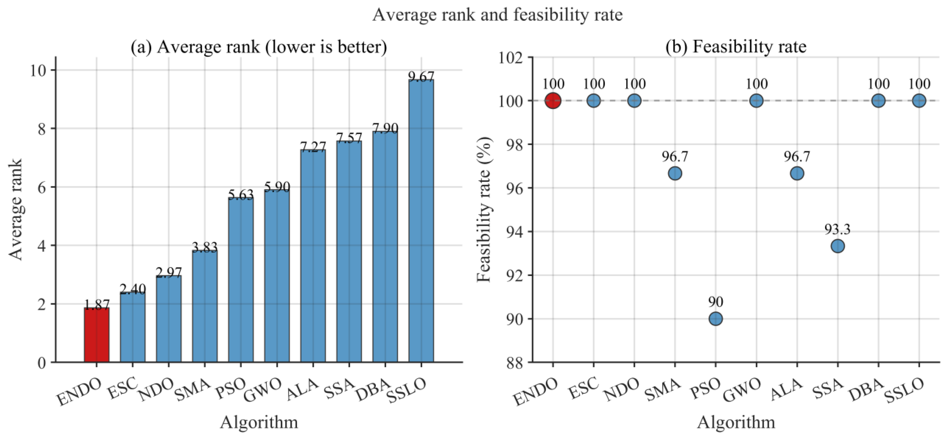
ENDO, ESC, NDO, GWO, DBA, and SSLO achieved feasibility rates of 100%, whereas the feasibility rates of SMA, ALA, SSA, and PSO were 96.7%, 96.7%, 93.3%, and 90.0%, respectively. Thus, a 100% feasibility rate was not unique to ENDO. Nevertheless, ENDO combined complete feasibility with the lowest mean operating cost and the best average rank.

DBA achieved the smallest standard deviation of 1.3960 × 10⁴, followed by ESC with 1.4907 × 10⁴, whereas the standard deviation of ENDO was 1.6805 × 10⁴. Therefore, ENDO did not produce the least dispersed results. However, its cost distribution remained concentrated in a relatively low-cost region, indicating a favorable balance between optimization accuracy and stability.

Figure 12 further illustrates the overall ranking and feasibility rates of the algorithms. ENDO ranks first with an average rank of 1.87, followed by ESC, NDO, and SMA. Combined with its 100% feasibility rate, this result shows that ENDO can maintain engineering feasibility while producing lower-cost scheduling solutions.

4.5.2. Convergence Behavior and Result Distribution

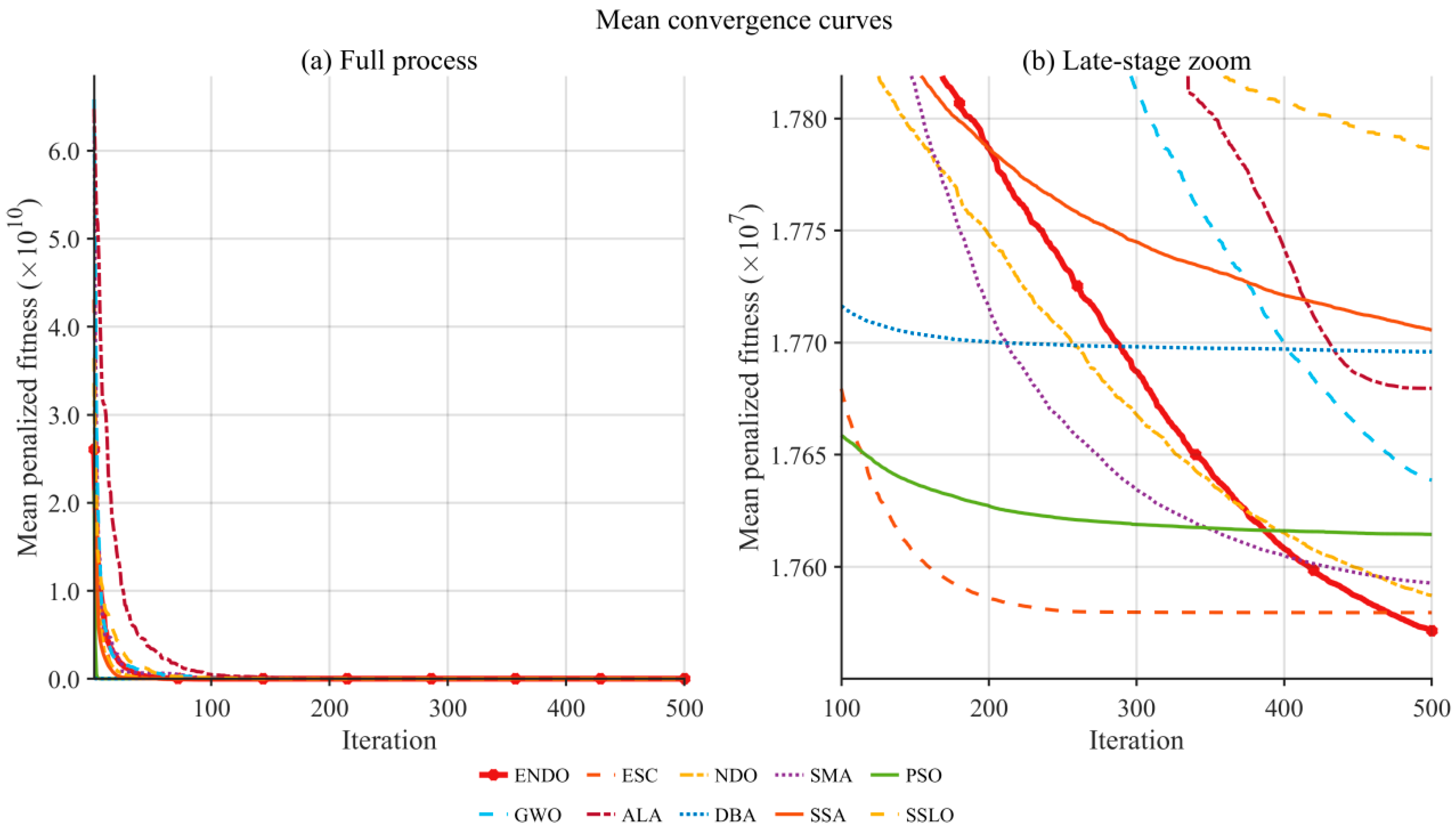
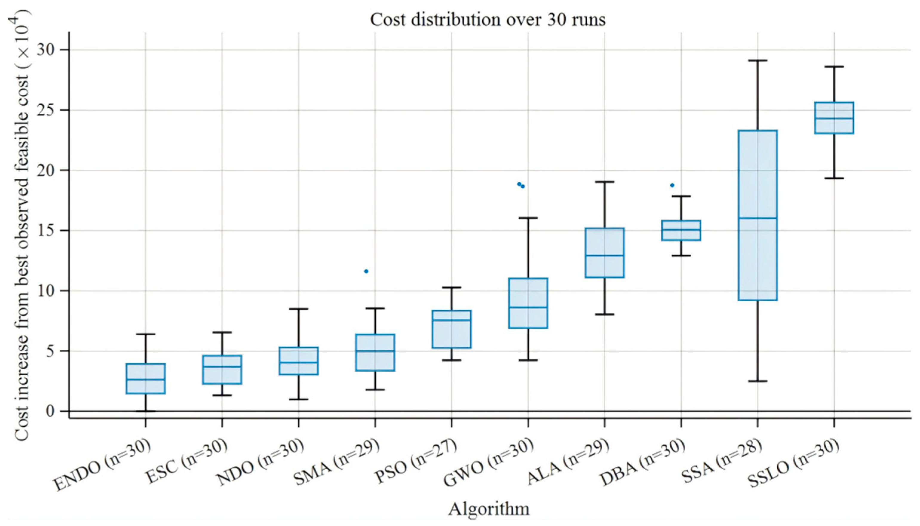
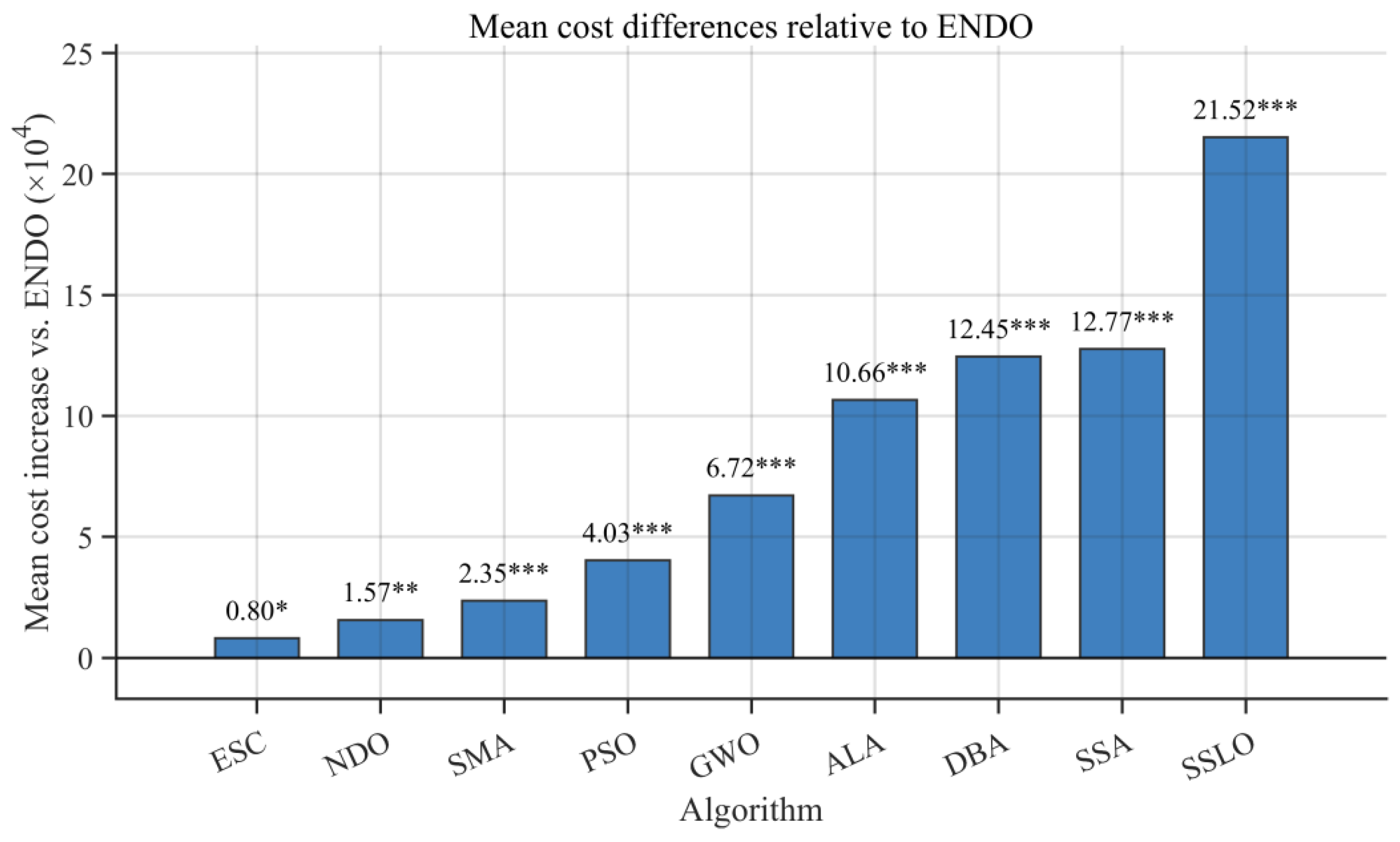
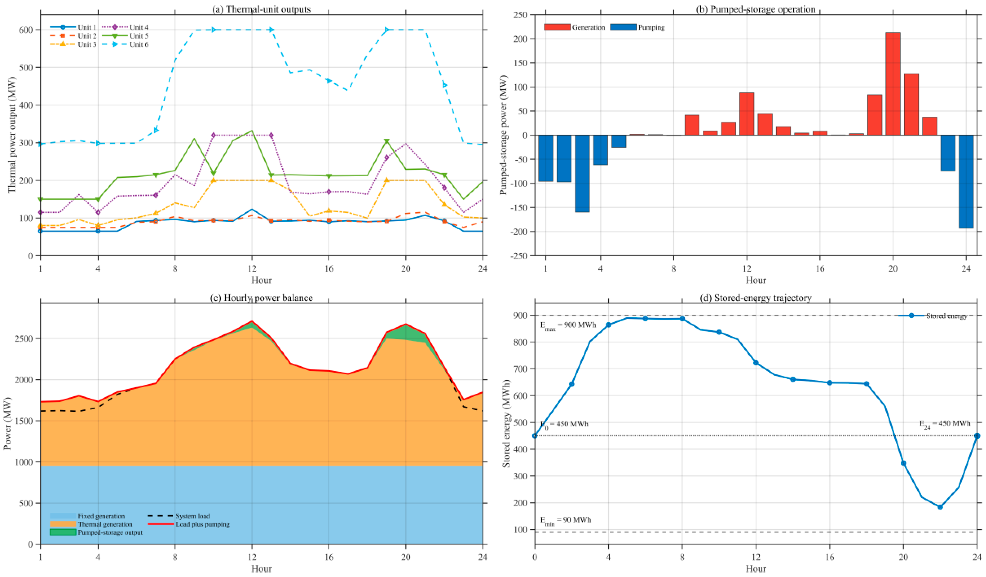
Figure 13 presents the mean best penalized fitness over 30 independent runs. The vertical axis represents penalized fitness rather than the unpenalized operating cost because it incorporates both the operating cost and the residual constraint penalties.

All algorithms rapidly reduced their penalized fitness during the early stage. ENDO did not remain dominant throughout the initial search, and algorithms such as ESC entered a low-fitness region earlier. However, the late-stage magnification shows that ENDO continued to improve its solutions during the middle and final stages and gradually became dominant after approximately 400 iterations. It eventually obtained the lowest mean penalized fitness. This behavior indicates that ENDO provides stronger sustained search and late-stage refinement capability rather than merely faster initial convergence.

As shown in Figure 14, the feasible operating costs obtained by the ten algorithms exhibit clear differences in both cost level and run-to-run variability. The vertical axis represents the increase in operating cost relative to the best feasible cost observed among all runs, while n denotes the number of feasible solutions obtained from the 30 independent runs. ENDO has the lowest median cost, and its interquartile interval is located in the lowest-cost region. ESC and NDO exhibit similar distributions, although their median costs remain slightly higher than that of ENDO. SSA shows the widest distribution, reflecting greater run-to-run variation. In contrast, SSLO produces a more concentrated distribution, but its operating costs are consistently higher.

The number of samples included for each algorithm depended on its feasibility rate. ENDO, ESC, NDO, GWO, DBA, and SSLO contributed 30 feasible runs; SMA and ALA contributed 29; SSA contributed 28; and PSO contributed 27. Therefore, the cost distributions should be interpreted together with the corresponding feasibility rates.

Figure 15 presents the paired mean cost differences between ENDO and the comparison algorithms. The differences were calculated by subtracting the operating cost obtained by ENDO from that obtained by each comparison algorithm, using only paired runs in which both algorithms produced feasible schedules. Therefore, a positive value indicates that ENDO achieved a lower operating cost. All paired mean differences were positive, demonstrating that ENDO outperformed every comparison algorithm in terms of mean operating cost over the paired feasible runs. The smallest difference was observed between ENDO and ESC, at 0.80 × 10⁴, whereas the largest difference was obtained between ENDO and SSLO, at 21.52 × 10⁴. The symbols ∗, ∗∗, and ∗∗∗ indicate statistically significant differences at p < 0.05, p < 0.01, and p < 0.001, respectively.

As shown in

Table 12. Paired Wilcoxon signed-rank comparison between ENDO and the other algorithms.

Compared Algorithm	Paired Feasible Runs	W/T/L	Mean Difference	Median Difference	p-Value
ESC	30	20/0/10	0.80 × 104	0.84 × 104	0.023038
NDO	30	21/0/9	1.57 × 104	1.63 × 104	0.001484
SMA	29	24/0/5	2.35 × 104	2.30 × 104	0.000124
PSO	27	26/0/1	4.03 × 104	3.78 × 104	6.28 × 10−6
GWO	30	29/0/1	6.72 × 104	6.22 × 104	2.35 × 10−6
ALA	29	29/0/0	10.66 × 104	11.07 × 104	2.56 × 10−6
DBA	30	30/0/0	12.45 × 104	12.70 × 104	1.73 × 10−6
SSA	28	28/0/0	12.77 × 104	12.32 × 104	3.79 × 10−6
SSLO	30	30/0/0	21.52 × 104	22.06 × 104	1.73 × 10−6

Note: W/T/L denotes the numbers of wins, ties, and losses of ENDO against the corresponding algorithm over the paired feasible runs.

, all Wilcoxon p-values were below 0.05, indicating statistically significant differences at the 5% level. Against ESC, ENDO achieved 20 wins and 10 losses, with a relatively small but statistically significant cost difference. Against ALA, DBA, SSA, and SSLO, ENDO won all 29, 30, 28, and 30 paired feasible runs, respectively, indicating a consistent cost advantage. Overall, the convergence curves, cost distributions, and statistical tests show that the primary advantage of ENDO lies in its sustained late-stage improvement, lower final cost, and reliable performance across repeated runs rather than in the fastest initial convergence.

4.5.3. Analysis of the Optimal Scheduling Scheme

Figure 16 presents the best thermal–pumped-storage scheduling scheme obtained by ENDO, including the hourly outputs of the six thermal units, the operation of the pumped-storage station, the hourly power balance, and the stored-energy trajectory.

As shown in Figure 16a, Unit 6 operates at relatively high output levels during most periods and reaches its maximum output of 600 MW during hours 10–13 and 19–21. Its output is also close to the upper limit during hour 9. This dispatch pattern is consistent with the relatively low normal operating-cost coefficient of Unit 6. Units 3–5 provide additional generation during high-load periods, whereas Units 1 and 2 generally operate at comparatively low output levels. The six thermal units coordinate their outputs in response to hourly load variations, and all unit outputs remain within their corresponding operating limits.

Figure 16b shows that the pumped-storage station mainly operates in pumping mode during hours 1–5 and 23–24 and in generation mode during hours 9–16 and 19–22, with only minor power exchanges during several remaining periods. Pumping during low-load periods converts electrical energy into stored energy, whereas generation during high-load periods reduces the thermal-generation requirement. This operating pattern reflects the peak-shaving, valley-filling, and energy-shifting functions of the pumped-storage station. Positive and negative values denote generation and pumping, respectively.

It should be noted that Figure 16b presents the pumped-storage power on the storage side. In contrast, the pumped-storage generation and pumping demand shown in Figure 16c are converted to the grid side using the corresponding generation and pumping efficiencies.

As illustrated in Figure 16c, the fixed-output sources continuously provide 950 MW, while the thermal units supply the principal adjustable generation. During pumping periods, the total demand exceeds the original system load because it includes the additional grid-side pumping consumption. During generation periods, the pumped-storage station contributes to the system power supply. The upper boundary of the stacked generation closely coincides with the total-demand curve throughout the scheduling horizon, confirming that the hourly power-balance constraint is satisfied.

Figure 16d shows that the stored energy increases from its initial value of 450 MWh to a maximum of approximately 889.62 MWh during the early pumping periods. It subsequently decreases as the pumped-storage station generates electricity during the high-load periods and reaches a minimum of approximately 183.19 MWh. The stored energy therefore remains within the allowable range of 90–900 MWh throughout the scheduling horizon. Pumping during hours 23 and 24 restores the stored energy to 450 MWh at the end of the scheduling horizon, thereby satisfying the daily-cycle constraint.

Overall, the best schedule obtained by ENDO effectively coordinates the thermal units and the pumped-storage station according to hourly load variations. The schedule stores energy during low-load periods and releases it during high-load periods while satisfying the thermal-output, hourly power-balance, stored-energy, and daily-cycle constraints. These results demonstrate the engineering rationality and practical feasibility of the scheduling scheme obtained by ENDO.

4.5.4. Constraint Satisfaction and Computational Efficiency

To further verify the engineering feasibility of the best scheduling scheme,

Table 13. Feasibility verification of the best scheduling solution obtained by ENDO.

Indicator	Obtained Value	Feasibility Criterion	Status
Operating cost	1.7543718 × 107	—	—
Penalty value	0	0	Satisfied
Maximum power-balance error	4.5475 × 10−13 MW	≤0.1 MW	Satisfied
Daily-cycle error	2.8422 × 10−14 MWh	≤0.1 MWh	Satisfied
Maximum general-constraint violation	0	≤0.2	Satisfied
Maximum stored-energy violation	0	≤0.2	Satisfied
Minimum stored energy	183.1933 MWh	≥90 MWh	Satisfied
Maximum stored energy	889.6220 MWh	≤900 MWh	Satisfied
Initial/terminal stored energy	450/450 MWh	E24 = E0	Satisfied

reports its principal constraint-related indicators. The reported operating cost corresponds to the unpenalized cost of the same feasible solution used to generate Figure 16.

As shown in Table 13, the best scheduling solution obtained by ENDO has an unpenalized operating cost of 1.7543718 × 10⁷ and a penalty value of zero. The maximum power-balance error and daily-cycle error are 4.5475 × 10⁻¹³ MW and 2.8422 × 10⁻¹⁴ MWh, respectively, both of which are substantially below the corresponding tolerance of 0.1. These extremely small residuals result from floating-point numerical calculations and can therefore be regarded as zero in practical terms.

The maximum violations of the general operating constraints and stored-energy constraints are both zero. Moreover, the stored energy varies from 183.1933 to 889.6220 MWh, remaining strictly within its allowable range of 90–900 MWh, and returns from its initial value of 450 MWh to the same value at the end of the scheduling horizon. These results confirm that the obtained schedule satisfies the thermal-output, ramping, spinning-reserve, stored-energy, hourly power-balance, and daily-cycle constraints.

In terms of computational efficiency, ENDO requires an average runtime of 58.784 s per independent run, which is the longest among the ten algorithms. By comparison, the average runtimes of NDO and PSO are 24.866 and 8.075 s, respectively. The additional search and candidate-evaluation operations incorporated into ENDO therefore increase its computational cost.

Nevertheless, the considered problem is a 24 h day-ahead scheduling task rather than a real-time control problem. An average computation time of approximately one minute is therefore acceptable for the corresponding scheduling time scale. Overall, although ENDO incurs additional computational cost, it achieves better results in terms of mean operating cost, average rank, and paired statistical performance. These results indicate that ENDO provides a reasonable balance between scheduling quality and computational efficiency for the considered thermal–pumped-storage dispatch problem.

5. Conclusions

This study developed an Enhanced Newton Downhill Optimizer (ENDO) by integrating an adaptive dimension mask, a DE/rand/2-based greedy mutation, and dynamic-boundary opposition-based guidance into the original NDO framework. These mechanisms regulate dimension-wise updating, provide additional search for lower-ranked individuals, and broaden the candidate source for global-best selection.

ENDO was evaluated on the CEC2017 benchmark at 10, 30, 50, and 100 dimensions. In the primary 100-dimensional comparison, it ranked first on 18 of 29 functions, achieved a top-three rank on 26 functions, and obtained an average rank of 1.79. Its mean fitness was lower than that of NDO on 28 functions. The average ranks at 10, 30, 50, and 100 dimensions were 1.79, 1.66, 1.38, and 1.79, respectively, indicating consistent performance across different problem scales. In the additional comparison with six advanced optimizers, ENDO ranked third with an average rank of 3.52 under the unified N/T protocol.

ENDO was further applied to a 168-dimensional thermal–pumped-storage economic dispatch problem. It achieved a 100% feasibility rate, the lowest mean operating cost, and the best average rank of 1.87 over 30 independent runs. The best schedule had an operating cost of 1.7543718 × 10⁷, zero penalty, and negligible power-balance and daily-cycle errors. All thermal-unit, ramping, reserve, storage, and terminal-cycle constraints were satisfied.

The additional mutation and opposition-based evaluations increase the computational cost relative to NDO. The function-evaluation budget analysis further demonstrated that the performance improvement of ENDO was not solely caused by the increased number of objective-function evaluations. Parameter sensitivity analysis showed that the selected control parameters provide stable performance, while population diversity and step-size analyses verified that the proposed mechanisms contribute to a better exploration–exploitation balance. Moreover, the engineering study considered a deterministic single-objective dispatch model. Future work will focus on reducing redundant evaluations and extending ENDO to uncertain renewable-energy scheduling, economic–emission dispatch, and larger integrated energy systems.

References

1. Boussaïd, I.; Lepagnot, J.; Siarry, P. A survey on optimization metaheuristics. Inf. Sci. 2013, 237, 82–117. [Google Scholar] [CrossRef] [Scilit]
2. Yang, X.S. Nature-inspired optimization algorithms: Challenges and open problems. J. Comput. Sci. 2020, 46, 101104. [Google Scholar] [CrossRef] [Scilit]
3. Alorf, A. A survey of recently developed metaheuristics and their comparative analysis. Eng. Appl. Artif. Intell. 2023, 117, 105622. [Google Scholar] [CrossRef] [Scilit]
4. Wolpert, D.H.; Macready, W.G. No free lunch theorems for optimization. IEEE Trans. Evol. Comput. 1997, 1, 67–82. [Google Scholar] [CrossRef] [Scilit]
5. Xiao, W.; Lian, J.J.; Ouyang, K.; Gu, S.; Ke, Z.; Wei, D.; Sha, X.; Wang, J.; Fu, S.; Qiu, M.; et al. Newton downhill optimizer with application to engineering optimization and breast cancer feature selection. Biomed. Signal Process. Control 2026, 117, 109184. [Google Scholar] [CrossRef] [Scilit]
6. Kennedy, J.; Eberhart, R. Particle swarm optimization. In Proceedings of the ICNN’95–International Conference on Neural Networks, Perth, Australia, 27 November–1 December 1995; Volume 4, pp. 1942–1948. [Google Scholar]
7. Poli, R.; Kennedy, J.; Blackwell, T. Particle swarm optimization: An overview. Swarm Intell. 2007, 1, 33–57. [Google Scholar] [CrossRef] [Scilit]
8. Mirjalili, S.; Mirjalili, S.M.; Lewis, A. Grey Wolf Optimizer. Adv. Eng. Softw. 2014, 69, 46–61. [Google Scholar] [CrossRef] [Scilit]
9. Xue, J.; Shen, B. A novel swarm intelligence optimization approach: Sparrow search algorithm. Syst. Sci. Control Eng. 2020, 8, 22–34. [Google Scholar] [CrossRef] [Scilit]
10. Li, S.; Chen, H.; Wang, M.; Heidari, A.A.; Mirjalili, S. Slime mould algorithm: A new method for stochastic optimization. Future Gener. Comput. Syst. 2020, 111, 300–323. [Google Scholar] [CrossRef] [Scilit]
11. Ouyang, K.; Fu, S.; Chen, Y.; Cai, Q.; Heidari, A.A.; Chen, H. Escape: An optimization method based on crowd evacuation behaviors. Artif. Intell. Rev. 2025, 58, 19. [Google Scholar] [CrossRef] [Scilit]
12. Xiao, Y.; Cui, H.; Abu Khurma, R.; Castillo, P.A. Artificial lemming algorithm: A novel bionic meta-heuristic technique for solving real-world engineering optimization problems. Artif. Intell. Rev. 2025, 58, 84. [Google Scholar] [CrossRef] [Scilit]
13. Ye, J.; Sunat, K.; Chiewchanwattana, S. Stochastic social learning optimization: Combining social learning and bucket theory for efficient optimization. Knowl.-Based Syst. 2026, 341, 115767. [Google Scholar] [CrossRef] [Scilit]
14. Cheng, J.; De Waele, W. Detective Behavior Algorithm (DBA): A new metaheuristic for design and engineering optimization. Knowl.-Based Syst. 2026, 338, 115434. [Google Scholar] [CrossRef] [Scilit]
15. Storn, R.; Price, K. Differential evolution–A simple and efficient heuristic for global optimization over continuous spaces. J. Glob. Optim. 1997, 11, 341–359. [Google Scholar] [CrossRef] [Scilit]
16. Brest, J.; Greiner, S.; Bošković, B.; Mernik, M.; Žumer, V. Self-adapting control parameters in differential evolution: A comparative study on numerical benchmark problems. IEEE Trans. Evol. Comput. 2006, 10, 646–657. [Google Scholar] [CrossRef] [Scilit]
17. Tizhoosh, H.R. Opposition-based learning: A new scheme for machine intelligence. In Proceedings of the International Conference on Computational Intelligence for Modelling, Control and Automation and International Conference on Intelligent Agents, Web Technologies and Internet Commerce, Vienna, Austria, 28–30 November 2005; Volume 1, pp. 695–701. [Google Scholar]
18. Rahnamayan, S.; Tizhoosh, H.R.; Salama, M.M.A. Opposition-based differential evolution. IEEE Trans. Evol. Comput. 2008, 12, 64–79. [Google Scholar] [CrossRef] [Scilit]
19. Lakbichi, R.; Zitouni, F.; Harous, S.; Ferhat, A.; Limane, A.; Almazyad, A.S.; Xiong, G.; Mohamed, A.W. Opposition-based learning techniques in metaheuristics: Classification, comparison, and convergence analysis. PeerJ Comput. Sci. 2025, 11, e2935. [Google Scholar] [CrossRef] [Scilit]
20. Gaing, Z.L. Particle swarm optimization to solving the economic dispatch considering the generator constraints. IEEE Trans. Power Syst. 2003, 18, 1187–1195. [Google Scholar] [CrossRef] [Scilit]
21. Park, J.B.; Jeong, Y.W.; Shin, J.R.; Lee, K.Y. An improved particle swarm optimization for nonconvex economic dispatch problems. IEEE Trans. Power Syst. 2010, 25, 156–166. [Google Scholar] [CrossRef] [Scilit]
22. Coelho, L.S.; Mariani, V.C. Combining of chaotic differential evolution and quadratic programming for economic dispatch optimization with valve-point effect. IEEE Trans. Power Syst. 2006, 21, 989–996. [Google Scholar] [CrossRef] [Scilit]
23. Nazari-Heris, M.; Mohammadi-Ivatloo, B.; Gharehpetian, G.B. Short-term scheduling of hydro-based power plants considering application of heuristic algorithms: A comprehensive review. Renew. Sustain. Energy Rev. 2017, 74, 116–129. [Google Scholar] [CrossRef] [Scilit]
24. Pozo, D.; Contreras, J.; Sauma, E.E. Unit commitment with ideal and generic energy storage units. IEEE Trans. Power Syst. 2014, 29, 2974–2984. [Google Scholar] [CrossRef] [Scilit]
25. Basu, M. Multi-region dynamic economic dispatch of solar–wind–hydro–thermal power system incorporating pumped hydro energy storage. Eng. Appl. Artif. Intell. 2019, 86, 182–196. [Google Scholar] [CrossRef] [Scilit]
26. Lu, M.; Guan, J.; Wu, H.; Chen, H.; Gu, W.; Wu, Y.; Ling, C.; Zhang, L. Day-ahead optimal dispatching of multi-source power system. Renew. Energy 2022, 183, 435–446. [Google Scholar] [CrossRef] [Scilit]
27. Chyong, C.K.; Newbery, D. A unit commitment and economic dispatch model of the GB electricity market—Formulation and application to hydro pumped storage. Energy Policy 2022, 170, 113213. [Google Scholar] [CrossRef] [Scilit]
28. Awad, N.H.; Ali, M.Z.; Liang, J.J.; Qu, B.Y.; Suganthan, P.N. Problem Definitions and Evaluation Criteria for the CEC 2017 Special Session and Competition on Single Objective Bound Constrained Real-Parameter Numerical Optimization; Technical Report; Nanyang Technological University: Singapore, 2016. [Google Scholar]
29. Hansen, N.; Ostermeier, A. Completely derandomized self-adaptation in evolution strategies. Evol. Comput. 2001, 9, 159–195. [Google Scholar] [CrossRef] [Scilit]
30. Tanabe, R.; Fukunaga, A. Success-history based parameter adaptation for Differential Evolution. In Proceedings of the 2013 IEEE Congress on Evolutionary Computation, Cancun, Mexico, 20–23 June 2013; pp. 71–78. [Google Scholar]
31. Tanabe, R.; Fukunaga, A.S. Improving the search performance of SHADE using linear population size reduction. In Proceedings of the 2014 IEEE Congress on Evolutionary Computation, Beijing, China, 6–11 July 2014; pp. 1658–1665. [Google Scholar]
32. Mohamed, A.W.; Hadi, A.A.; Fattouh, A.M.; Jambi, K.M. LSHADE with semi-parameter adaptation hybrid with CMA-ES for solving CEC 2017 benchmark problems. In Proceedings of the 2017 IEEE Congress on Evolutionary Computation, Donostia, Spain, 5–8 June 2017; pp. 145–152. [Google Scholar]
33. Kumar, A.; Misra, R.K.; Singh, D. Improving the local search capability of Effective Butterfly Optimizer using Covariance Matrix Adapted Retreat Phase. In Proceedings of the 2017 IEEE Congress on Evolutionary Computation, Donostia, Spain, 5–8 June 2017; pp. 1835–1842. [Google Scholar]
34. Brest, J.; Sepesy Maučec, M.; Bošković, B. Single objective real-parameter optimization: Algorithm jSO. In Proceedings of the 2017 IEEE Congress on Evolutionary Computation, Donostia, Spain, 5–8 June 2017; pp. 1311–1318. [Google Scholar]
35. Wilcoxon, F. Individual comparisons by ranking methods. Biom. Bull. 1945, 1, 80–83. [Google Scholar] [CrossRef] [Scilit]
Figure 1. Flowchart of the proposed ENDO algorithm.
Algorithms 19 00761 g001
Figure 2. Mean convergence curves of ENDO and the compared algorithms on the 100-dimensional CEC2017 functions F1 and F3F10.
Algorithms 19 00761 g002
Figure 3. Mean convergence curves of ENDO and the compared algorithms on the 100-dimensional CEC2017 functions F11F20.
Algorithms 19 00761 g003
Figure 4. Mean convergence curves of ENDO and the compared algorithms on the 100-dimensional CEC2017 functions F21F30.
Algorithms 19 00761 g004
Figure 5. Boxplots of ENDO and the compared algorithms on the 100-dimensional CEC2017 functions F1 and F3F10. The central line indicates the median, the box represents the interquartile range, the whiskers indicate the non-outlier range, and circles denote outliers.
Algorithms 19 00761 g005
Figure 6. Boxplots of ENDO and the compared algorithms on the 100-dimensional CEC2017 functions F11F20. The central line indicates the median, the box represents the interquartile range, the whiskers indicate the non-outlier range, and circles denote outliers.
Algorithms 19 00761 g006
Figure 7. Boxplots of ENDO and the compared algorithms on the 100-dimensional CEC2017 functions F21F30. The central line indicates the median, the box represents the interquartile range, the whiskers indicate the non-outlier range, and circles denote outliers.
Algorithms 19 00761 g007
Figure 8. Function-wise ranking radar charts of the compared algorithms on the 100-dimensional CEC2017 benchmark: (a) F1 and F3–F15; (b) F16–F30.
Algorithms 19 00761 g008
Figure 9. Average rankings of the compared algorithms on the 100-dimensional CEC2017 benchmark.
Algorithms 19 00761 g009
Figure 10. Dynamic variations of population diversity and average step size for different algorithm variants on representative benchmark functions. (ad) correspond to F11 population diversity, F11 average step size, F15 population diversity, and F15 average step size, respectively.
Algorithms 19 00761 g010
Figure 11. Heatmap of the average rankings of the compared algorithms across different dimensions. The red box highlights the results of ENDO.
Algorithms 19 00761 g011
Figure 12. Average rank and feasibility rate of the compared algorithms.
Algorithms 19 00761 g012
Figure 13. Mean convergence curves of the compared algorithms: (a) overall convergence process; (b) late-stage magnification.
Algorithms 19 00761 g013
Figure 14. Distribution of feasible operating costs obtained by the ten algorithms over 30 independent runs.
Algorithms 19 00761 g014
Figure 15. Paired mean cost differences between ENDO and the comparison algorithms. ∗, ∗∗, and ∗∗∗ indicate statistically significant differences at p < 0.05, p < 0.01, and p < 0.001, respectively.
Algorithms 19 00761 g015
Figure 16. Best thermal–pumped-storage scheduling scheme obtained by ENDO.
Algorithms 19 00761 g016