A Transfer Learning and Data Augmentation Approach for Classifying Field Images of Granite Residual Slope Soils

Abstract

Granite residual and slope-wash soils are important disaster-prone geological bodies in the hilly and mountainous areas of Hunan Province, China. Their engineering classification has long relied on manual visual inspection and laboratory testing, which is inefficient and subjective. In this study, an automatic classification method based on deep learning image recognition is proposed for granite residual and slope-wash soils in the mountainous areas of Hunan Province. First, a three-class primary classification scheme was established, comprising residual clay (RNC), residual sandy clay (RNSC), and residual gravelly clay (RNGC), based primarily on the gravel content of particles larger than 2 mm (RNC < 5%, RNSC 5–20%, RNGC > 20%). Second, 7678 geotechnical test records from 21 counties in Hunan Province were collected, and classification labels were assigned through a strategy combining manual verification and automatic inference using Random Forest (5-fold cross-validation macro F1 = 0.913). From approximately 10,096 original field images, 3380 pure soil image patches were retained after segmentation and screening. A dataset of 43,940 samples was then generated through two-stage preprocessing (including denoising and illumination correction) and 13-fold data augmentation. A CNN image classification model was constructed based on a ResNet18 backbone network pre-trained on ImageNet. On the independent test set (6591 images), the primary classification accuracy reached 91.46%, with a macro F1-score of 0.9128; the per-class F1-scores for RNC, RNSC, and RNGC were 0.921, 0.885, and 0.933, respectively. Grad-CAM visualization analysis demonstrated that the model’s attention was primarily focused on soil particle distribution regions rather than non-soil background areas, confirming the effective learning of mixed-grain features. The study shows that the combined application of transfer learning and 13-fold data augmentation can significantly improve classification performance under limited sample size conditions (an improvement of 15.33 percentage points compared to the baseline of 76.13%), demonstrating promising potential for engineering applications.

1. Introduction

Granite residual and slope-wash soils are widely distributed in the hilly and mountainous areas of South China, including Hunan, Guangdong, and Fujian provinces. They serve as the primary foundation-bearing strata for buildings and structures in these regions and constitute important disaster-prone geological bodies for shallow landslides, debris flows, and other geological hazards [1]. In Hunan Province, the engineering geological properties of these soils exhibit significant variability, with hundreds of geological disasters induced by differences in residual soil engineering properties occurring annually. However, the engineering classification and identification of these soils still primarily rely on field visual inspection by surveyors or laboratory geotechnical testing. The former is significantly influenced by subjective experience and lacks consistency, while the latter, despite providing precise results, involves lengthy sample preparation and testing cycles that cannot meet the practical demands of large-scale, fast-paced geological hazard screening and engineering surveys. In recent years, deep learning-based general image classification techniques have demonstrated strong potential in agricultural soil identification [2], rock and mineral material recognition, and other fields [3,4], offering a new technical approach for the rapid and objective identification of granite residual soils. However, research specifically targeting this particular soil type, especially its field in situ images, remains in its nascent stage.

In terms of fundamental research on granite residual soils, Wu [1] pointed out from a structural perspective that these soils are typical “mixed-grain soils,” whose engineering properties are jointly controlled by both coarse and fine particle fractions, rendering traditional single-index classification methods significantly limited. Zhuang et al. [5] further utilized X-ray micro-focus CT technology to reveal the microstructural characteristics of different types of granite residual soils, providing micro-scale evidence for understanding their macroscopic mechanical behavior. Li et al. [6] additionally characterized the three-dimensional microstructure of particles and moisture morphology in granite residual soils. The aforementioned studies have established a solid theoretical foundation in soil mechanics but also indicate that rapid field identification solely through traditional laboratory testing is difficult, highlighting the urgent need for new technical approaches.

Significant progress has been made in the frontier exploration of deep learning applied to geotechnical image recognition. A systematic review by Pal and Gupta [4] indicated that lightweight convolutional neural networks (CNNs) combined with transfer learning have become the mainstream trend in this field. Jalapur et al. [3] systematically evaluated the performance of various backbone networks, including EfficientNetB0 and ResNet50, in soil image classification, verifying the favorable balance between accuracy and efficiency achieved by transfer learning. Yan et al. [7] applied CNNs to red bed soft rock identification, preliminarily exploring the feasibility of deep learning in geotechnical engineering. Abdullah et al. [8] proposed a novel lightweight CNN (RockDNet) for lithology classification of carbonate, sandstone, and shale, achieving high accuracy with over 98% parameter reduction compared to benchmark models. In the specialized target recognition of geological materials, Hu et al. [9] constructed an automatic rock lithology classification model based on ResNet18 transfer learning, achieving a recognition accuracy of 96.10% for six rock types including granite and marble. Li et al. [10] improved the DenseNet algorithm for cone penetration test (CPT) soil layer classification, also achieving a recognition rate of 92.09%. Furthermore, Zohouri Rad et al. [11] introduced Vision Transformer into soil classification, reaching an accuracy of 95.83% on a self-constructed dataset, demonstrating the potential of more complex network architectures. In terms of data augmentation and model tuning, Feng [12] explored the enhancement effects of color augmentation methods such as CLAHE and Gamma correction on geotechnical image recognition; Ma et al. [13] focused on CNN recognition patterns for rock thin section images; Chen et al. [14] proposed a pre-computed Gaussian process subspace method to accelerate Bayesian hyperparameter optimization, providing a new scheme for model training efficiency optimization.

Although the aforementioned studies have confirmed the feasibility of deep learning methods for geotechnical material recognition, three significant shortcomings remain regarding granite residual and slope-wash soils as a specific target: First, there is a mismatch in research objects—existing classification models mostly target general soil types (sand/silt/clay) or single lithologies, lacking specialized feature extraction schemes designed for the “mixed-grain” grading characteristics of granite residual soils. Second, data sources are limited—the vast majority of model validations are based on laboratory standard specimens or thin section images, and no representative field in situ image dataset has been established, making it difficult to reflect complex interferences such as uneven illumination and surface disturbance in real scenarios. Third, strategy evaluation is fragmented—the independent contributions and synergistic effects of transfer learning and small-sample data augmentation in real field scenarios have not been systematically quantified.

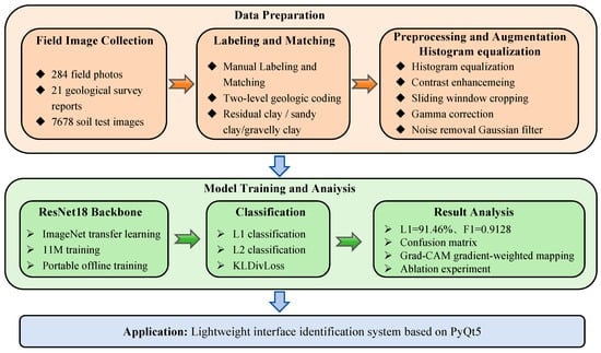
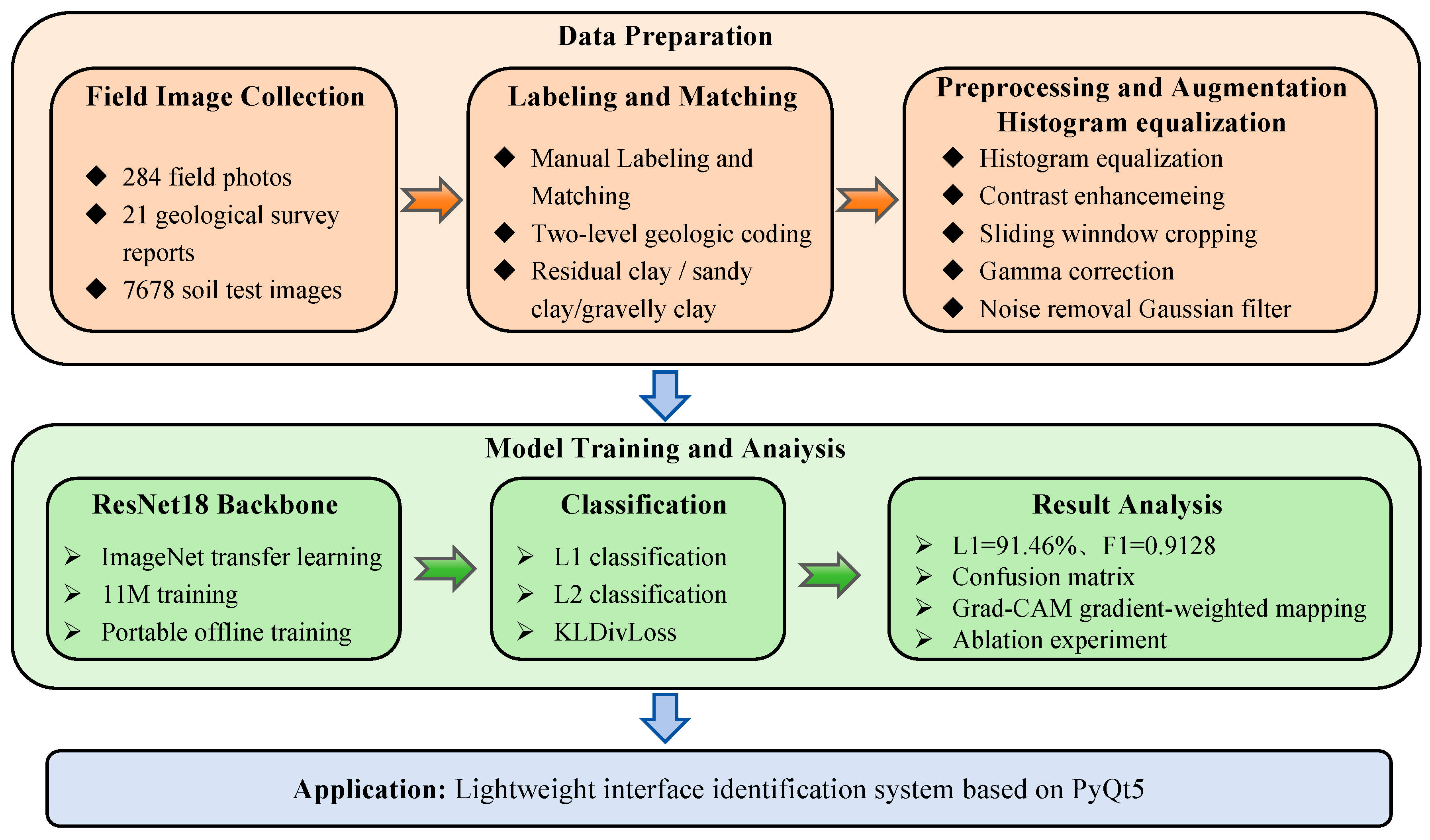
To address the aforementioned bottlenecks, this study focuses on the rapid and objective engineering classification of granite residual and slope-wash soils in the mountainous areas of Hunan Province. The main contributions are reflected in the following three aspects. The methodological framework is shown in Figure 1.

Figure 1. Methodological framework.

First, the initial field in situ image and geotechnical test label paired dataset covering 21 counties in Hunan Province for granite residual and slope-wash soils was established. Through joint calibration of field surveys and laboratory testing, the gap in field image sample libraries for mixed-grain soils was filled, providing a data foundation for subsequent similar studies.

Second, a small-sample classification framework based on ResNet18 transfer learning was constructed, with targeted image preprocessing and augmentation strategies designed to adapt to complex field illumination environments, effectively mitigating model overfitting. Meanwhile, Grad-CAM interpretability analysis was introduced to visually verify the model’s effective attention to “mixed-grain” key features, enhancing credibility from a geological perspective.

Third, through systematic ablation experiments, the respective contributions and synergistic gain effects of transfer learning weights and data augmentation strategies were quantitatively decomposed, providing empirical evidence for strategy selection in small-sample geological image classification. Additionally, a lightweight desktop recognition system based on PyQt5 was developed, preliminarily verifying the feasibility and promotion value of deploying this method in actual field surveys.

2. Materials and Methods

2.1. CNN Model Architecture and Training Strategy

2.1.1. Model Architecture

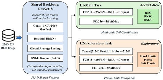
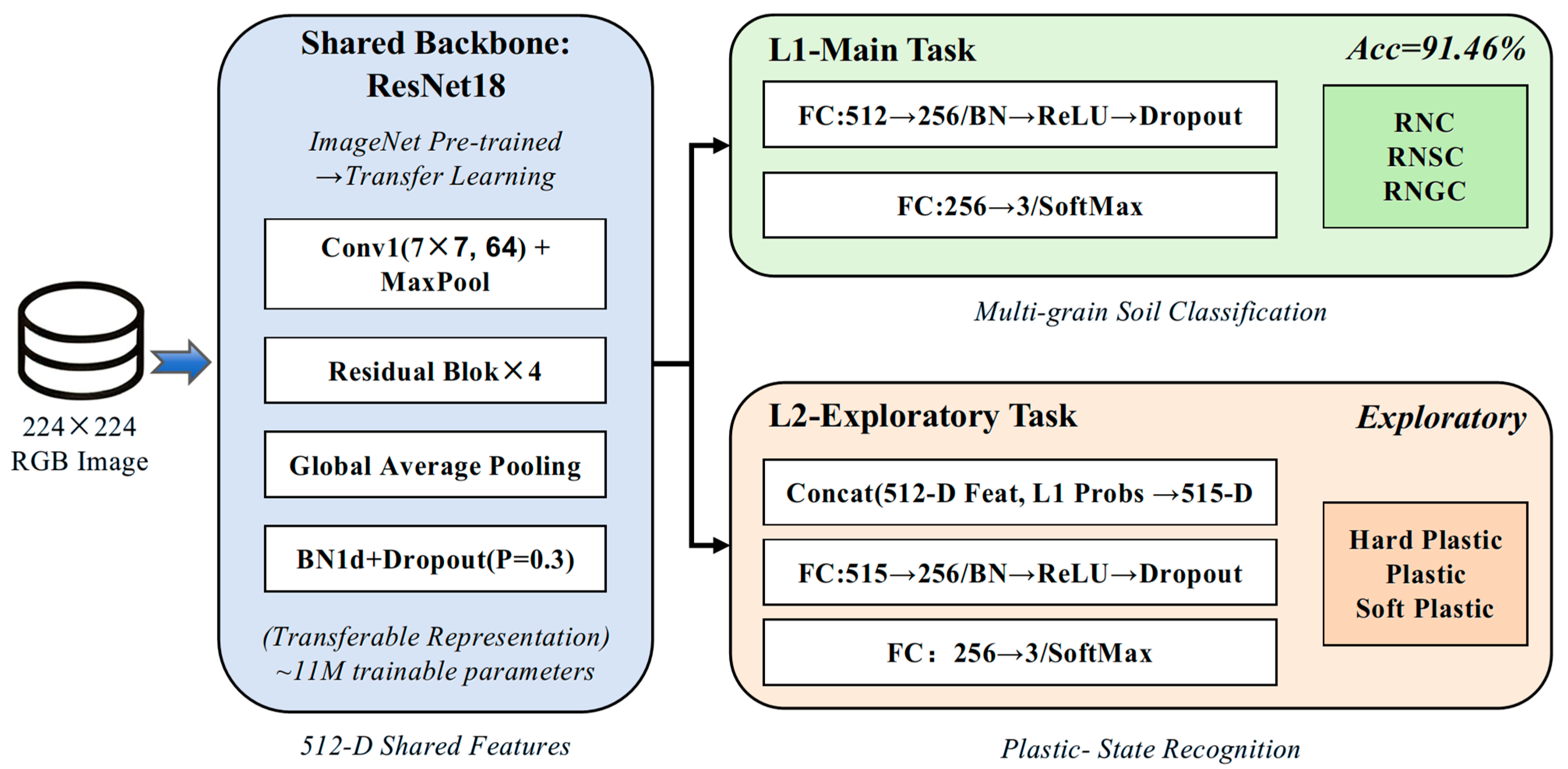
This study employs ResNet18 [15] as the backbone network, using ImageNet pre-trained weights for transfer learning (Figure 2). The model consists of three modules: a shared backbone network, a Level-1 classification head (L1-Head), and a Level-2 classification head (L2-Head). The Level-1 classification aims to recognize the mixed-grain characteristics of granite residual and slope-wash soils, including residual clay (RNC), residual sandy clay (RNSC), and residual gravelly clay (RNGC), which constitutes the core task of this study. The Level-2 classification serves as an exploratory experiment to evaluate the potential of using single visible-light images to discriminate the plastic state (hard plastic, plastic, and soft plastic) of soils.

Figure 2. Architecture of multi-task CNN based on ResNet18.

Given that this task is only a three-class classification problem with significantly lower complexity than ImageNet’s 1000-class task, the approximately 11 M parameters of ResNet18 are sufficient to represent the feature differences between classes. Therefore, larger parameter models such as ResNet50/101 were abandoned to reduce overfitting risk under small-sample conditions and to meet the requirements for model lightweight and real-time inference in field deployment.

The shared backbone network outputs a 512-dimensional feature vector, followed by batch normalization and Dropout (p = 0.3) to prevent overfitting. The Level-1 classification head consists of a fully connected layer (512→256), batch normalization, ReLU activation, and Dropout, ultimately mapping to 3-dimensional logits. The exploratory Level-2 classification head concatenates the 512-dimensional backbone features with the gradient-detached (detach) Level-1 Softmax probabilities (3-dimensional) to form a 515-dimensional input vector, which is then mapped to 3-dimensional logits through a structurally similar fully connected layer (515→256) to explore the potential association between plastic state and visual features.

2.1.2. Loss Function and Training Strategy

The Level-1 classification task employs weighted cross-entropy loss to mitigate class imbalance. Statistically, the sample quantities of the three classes (RNC, RNSC, and RNGC) are nearly balanced, with corresponding class weights of 1.06, 1.02, and 0.93, all close to 1.0. Thus, the weighting operation has minimal impact on the overall loss magnitude, primarily serving to maintain the generality of the methodological framework.

The Level-2 classification, as an exploratory task, employs KL divergence soft-label loss (Kullback–Leibler Divergence Loss). The soft labels are not derived from manual hard coding but are generated based on the statistical distribution of the liquidity index (IL) of each sample: according to the plastic state classification thresholds in the Code for Geotechnical Engineering Investigation (hard plastic: IL ≤ 0; plastic: 0 < IL ≤ 0.75; soft plastic: IL > 0.75), the reciprocal of the normalized distance from each sample’s IL value to each threshold interval is used as the weight to construct 3-dimensional probability soft labels. This approach better expresses the uncertainty of samples near plastic state boundaries and avoids the information loss caused by hard label division.

The total loss function is composed of the two loss terms with equal weights (λ1 = λ2 = 1.0). It should be noted that, through pre-experimental monitoring, the Level-1 cross-entropy loss and Level-2 KL divergence loss were found to be of comparable numerical magnitude during training (both in the range of 0.5–1.5), and thus no additional dynamic weight balancing mechanism was introduced.

The training hyperparameters are shown in Table 1. The AdamW optimizer was selected with an initial learning rate of 1 × 10⁻⁴, and a cosine annealing learning rate scheduling strategy was adopted, combined with a 3-epoch linear warmup phase to stabilize the AdamW adaptive momentum statistics and avoid gradient update instability during the initial training phase. To conserve GPU memory, gradient accumulation steps were set to 2 (original batch_size = 16, equivalent batch_size = 32). During training, model checkpoints were saved every 3 epochs, and early stopping was triggered if the validation loss did not decrease for 15 consecutive epochs, to select the optimal generalization model.

Table 1. Training hyperparameters of ResNet18 v2.

Hyperparameter	Value	Description
Input size	224 × 224	Standard ResNet input
Batch size	16 (equiv. 32)	Gradient accumulation steps = 2
Optimizer	AdamW	weight_decay = 1 × 10−4
Initial learning rate	1 × 10−4	Cosine annealing to 0
LR schedule	Cosine annealing	Warmup for first 3 epochs
Epochs	25	Best model at epoch 25
Early stopping patience	15	Based on validation L1 accuracy
Backbone pre-training	ImageNet	Transfer learning
Hardware	GTX 1050 Ti (4 GB VRAM)	CUDA 10.2

2.1.3. Model Interpretability Analysis Method

To verify whether the model’s attention to the mixed-grain characteristics of granite residual and slope-wash soils is geologically reasonable, and to rule out the possibility that the model relies on non-geological surface cues such as background and shadows, this study employs Gradient-Weighted Class Activation Mapping (Grad-CAM) [16] to visualize the model’s decision regions. Grad-CAM calculates the gradient of the predicted class score with respect to the feature maps of the last convolutional layer, applies global average pooling to obtain channel importance weights, and, after weighted summation and ReLU activation, upsamples to the same size as the input image (224 × 224), generating a heatmap that reflects the model’s attention regions.

In the specific implementation, the output feature maps of the last convolutional layer in the ResNet18 backbone (i.e., the convolutional layer in the last BasicBlock of layer4, layer4.1.conv2) were selected as the visualization target. By comparing the correspondence between the heatmap and the positions of gravel distribution and particle enrichment regions in the original image, it can be qualitatively determined whether the model has established visual associations related to grain size composition, rather than merely recognizing simple background patterns. In this study, Grad-CAM visualization was implemented via the pytorch-grad-cam open-source toolbox, with the target layer specified as layer4.1.conv2 of the ResNet18 backbone.

2.1.4. Experimental Environment

The model training and testing in this study were all completed on a laptop equipped with an NVIDIA GeForce GTX 1050 Ti graphics card (4 GB VRAM). The software environment includes the Windows 10 operating system, PyTorch 1.10.2 (CUDA 10.2) deep learning framework, and Python 3.8 programming language. Image preprocessing and data loading rely on OpenCV and the native PyTorch DataLoader interface, respectively. Mixed precision training (torch.cuda.amp) was employed during training to reduce memory usage, and the DataLoader’s num_workers was set to 4 to enable multi-process data pre-loading for improved GPU utilization.

2.2. Classification Scheme Design

The engineering classification methods for granite residual and slope-wash soils mainly include three categories: particle gradation method, plasticity index method, and field description method [1]. The particle gradation method uses particle group content as the classification criterion, offering strong operability and good alignment with current standards (GB/T 50145—2007 [17]; GB 50021—2001 (2009 edition) [18]). However, the threshold values for classifying particle group content lack unified standards, involving a certain degree of subjective determination, and the influence of plastic state is not fully considered. The plasticity index method, based on the consistency characteristics of fine-grained soils, is suitable for indoor identification but ignores the contribution of coarse particle content to the special mixed-grain characteristics of granite residual soils [1]. The field description method facilitates rapid field application but is highly subjective, poorly reproducible, and difficult to systematically associate with laboratory test data.

Given these limitations, a single classification method cannot adequately address the dual control role of both coarse and fine particle fractions in granite residual and slope-wash soils. This study establishes a two-level comprehensive classification system with particle gradation as the primary classification criterion and plastic state as the auxiliary subdivision criterion (Table 2). The selection of particle gradation as the core indicator for Level-1 classification is primarily based on the “mixed-grain” nature of granite residual and slope-wash soils—their macroscopic engineering properties (strength, compressibility, and permeability) are primarily determined by the relative content ratio of coarse particles (gravel) to fine particles (clay/silt), and gradation characteristics determine the soil skeleton structure. Plastic state, on the other hand, mainly reflects the consistency fluctuation caused by moisture content changes in the fine particle fraction, representing a further subdivision within the same gradation type.

Table 2. Comprehensive classification scheme of granite residual soil.

Class No.	Class Name (Abbrev.)	Gravel Content (>2 mm)	Sand Content (0.075–2 mm)	Fines Content (<0.075 mm)
I	Residual Clay (RNC)	<5%	<30%	>60%
II	Residual Sandy Clay (RNSC)	5–20%	30–50%	30–60%
III	Residual Gravelly Clay (RNGC)	>20%	>40%	<40%
Sub-class	Hard Plastic/Plastic/Soft Plastic	Based on IL	IL ≤ 0.25/0.25–0.75/>0.75	—

Note: Particle contents are expressed as mass percentages. Thresholds reference GB/T 50145-2007 [15] and the classification framework of Wu [1], and are determined in conjunction with the statistical results of measured data of Hunan granite residual and slope-wash soils in this study.

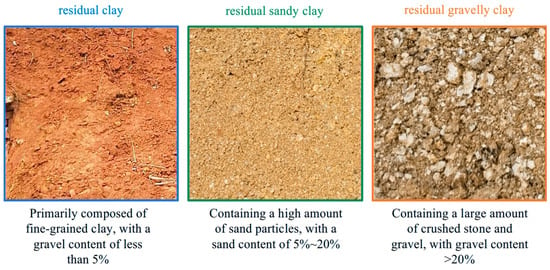
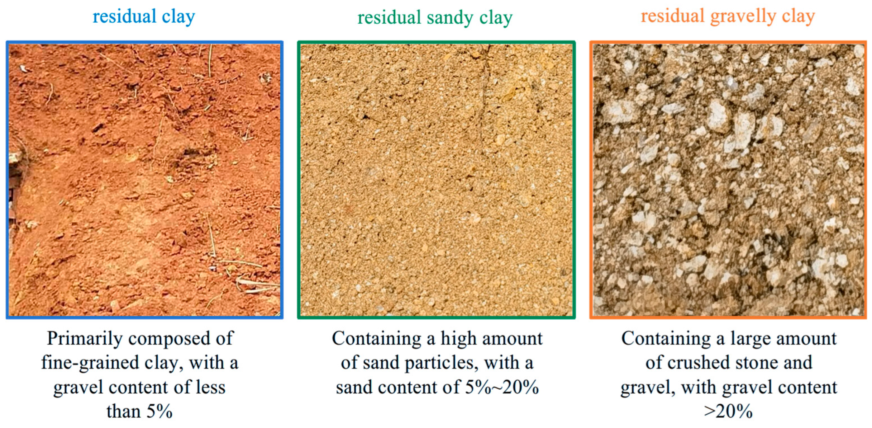
The Level-1 classification uses the gravel content of particles larger than 2 mm as the core discriminating indicator (Figure 3), dividing granite residual and slope-wash soils into three categories: residual clay (RNC), residual sandy clay (RNSC), and residual gravelly clay (RNGC). The Level-2 classification further subdivides each category into three sub-classes based on the liquidity index (IL).

Figure 3. Typical field photographs of three types of granite residual soil.

2.3. Dataset Construction

Granite residual and slope-wash soils in Hunan Province are widely distributed across six regions: northeastern, eastern, southeastern, central, southwestern, and southern Hunan, covering 11 prefecture-level cities including Yueyang, Changsha, Zhuzhou, and Chenzhou, and 63 counties. The geotechnical test data and field in situ image data in this study were sourced from 21 of these counties.

2.3.1. Geotechnical Test Dataset

The geotechnical test data were sourced from geotechnical engineering survey reports from 21 counties in Hunan Province, with a total of 7678 valid records collected, covering 14 physical and mechanical indicators including moisture content, natural density, specific gravity of soil particles, void ratio, degree of saturation, liquid limit, plastic limit, plasticity index, liquidity index, compression coefficient, compression modulus, cohesion, friction angle, and content of particles larger than 2 mm (Figure 4). Data extraction was performed using programmatic batch parsing, with separate extraction scripts written for structured tables embedded in Word documents, significantly improving data collection efficiency. The original data were subjected to quality control procedures including format standardization, deduplication, and outlier removal to retain valid records.

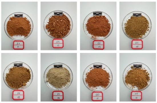
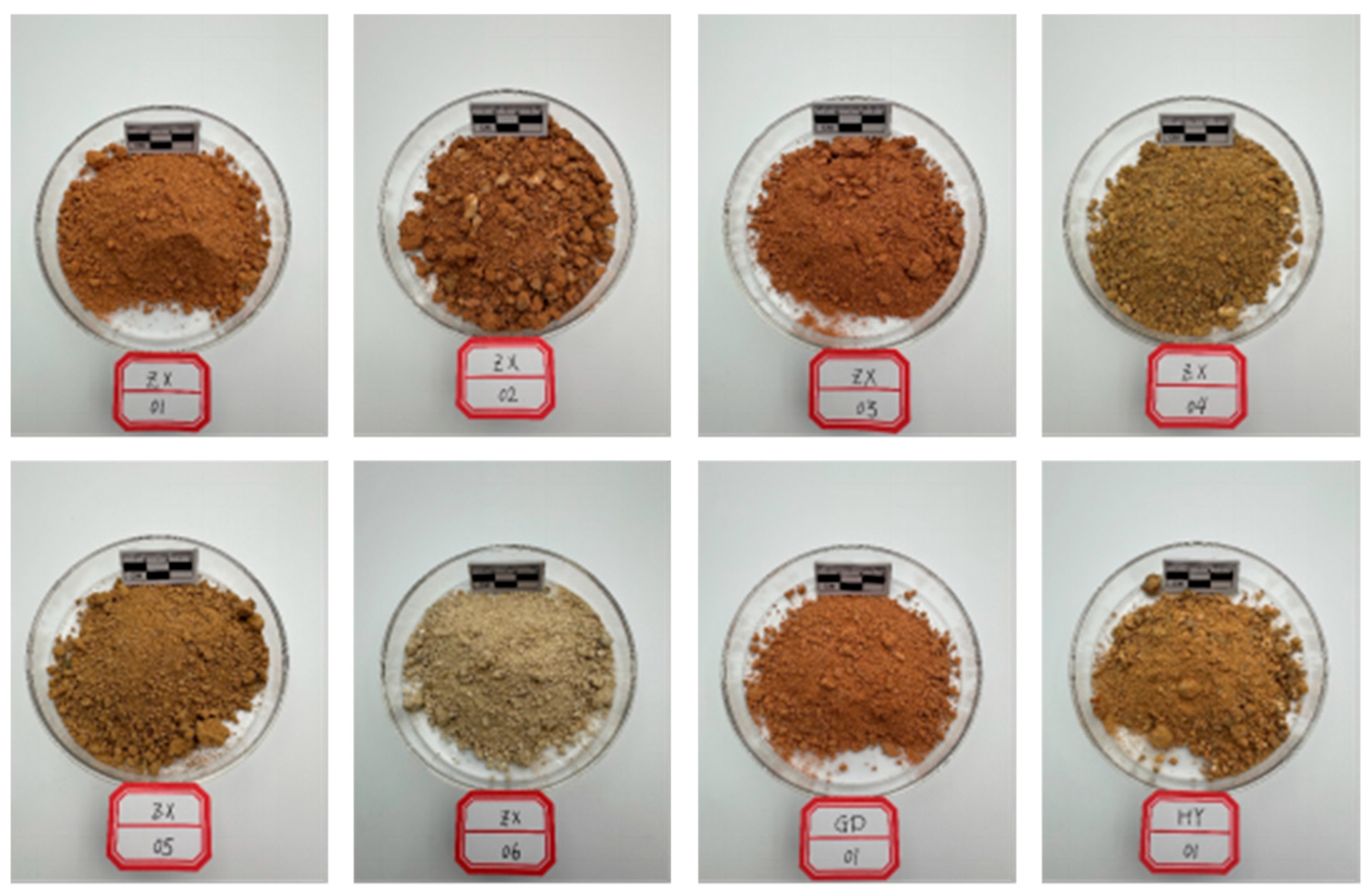
Figure 4. Typical scattered soil samples from landslide slopes of granite residual soil in field sites.

The original survey reports only contained geotechnical nomenclature descriptions and lacked classification labels quantitatively defined according to the classification system of this study (Section 2.2). Therefore, a two-stage labeling strategy of “manual verification + machine learning automatic inference” was adopted. In the first stage, 1023 samples were manually verified and labeled by professional geological personnel, using the content of particles larger than 2 mm as the core discriminating criterion (comprehensively referencing the field naming descriptions in the reports). Labeling was conducted using stratified sampling by county to ensure broad spatial coverage, while also considering class balance. The labeling results covered three categories: RNC (789 samples, 77.1%), RNSC (95 samples, 9.3%), and RNGC (139 samples, 13.6%). In the second stage, a Random Forest classifier was used for automatic labeling of the remaining unlabeled samples, an approach validated by recent studies on RF-based soil classification [19]. It should be particularly noted that, to ensure the effectiveness of the labeling method rather than simple lookup, the input features of the Random Forest did not include the classification-defining core indicator (content of particles larger than 2 mm), but instead used 13 physical and mechanical indicators including moisture content, natural density, specific gravity of soil particles, void ratio, degree of saturation, liquid limit, plastic limit, plasticity index, liquidity index, compression coefficient, compression modulus, cohesion, and friction angle for indirect inference. Among these, natural density had a high missing rate (75.2%), so an additional binary indicator feature was added to mark whether this field was missing, with missing values filled with 0, resulting in a final input dimensionality of 14.

Through 5-fold cross-validation on the training set, the Random Forest model achieved a macro F1-score of 0.913 and a balanced accuracy of 0.966, consistent with the competitive performance of RF reported in recent comparative studies [20], with the class-wise validation results shown in Table 3. Although RNGC had the fewest samples, its F1-score still reached 0.83 due to its clear particle content characteristics, indicating reliable classification results. After automatic labeling, the class distribution was adjusted from the manual labeling stage’s RNSC proportion of 9.3% to 20.4%, which is closer to the prevalence proportion of this soil type in regional geological data of Hunan Province. This indicates that a certain sampling bias existed during the manual labeling stage, and the Random Forest’s joint inference based on multiple indicators effectively corrected this bias. It should be clarified that the 7678 records refer to the total number of collected geotechnical test records, whereas the 5-fold cross-validation (and hence the support values in Table 3) was conducted on the 6012 training samples that carried verified labels and satisfied the feature-availability criterion (at least three of the twelve core indicators available). Of the remaining 1666 records, 636 met the minimum criterion for automatic inference (at least two available core indicators) and were assigned labels by the final fitted model, while the 1030 records with fewer than two available indicators were retained in the database without three-class labels. The final labeled dataset therefore comprised 6648 records, including 5138 RNC (77.3%), 1354 RNSC (20.4%), and 156 RNGC (2.3%).

Table 3. Classification metrics of each category based on 5-fold cross-validation of Random Forest.

Class	Precision	Recall	F1-Score	Support
RNC	1.00	0.97	0.98	5105
RNSC	0.84	0.95	0.89	758
RNGC	0.74	0.96	0.83	149
Macro avg.	0.86	0.96	0.90	6012

Note: The 5-fold cross-validation was conducted on the 6012 labeled training samples that satisfied the feature-availability criterion (at least three of the twelve core indicators available); the support values therefore sum to 6012 rather than the 7678 collected records. See Section 2.3.1 for the complete sample accounting.

The detailed configuration of the Random Forest labeling model is summarized below. Implemented in scikit-learn v0.24.2, the classifier was set with n_estimators = 300, max_depth = 8, and class_weight = “balanced”, with a fixed random seed (random_state = 42) for full reproducibility; all other parameters were kept at default values. This configuration was selected after preliminary comparison against logistic regression and gradient boosting models via Bayesian optimization, where the Random Forest achieved the highest cross-validated macro-F1 score.

For preprocessing and missing value handling, records with fewer than three valid core indicators were excluded from model training, and those with fewer than two were excluded from automatic inference. Missing values for the twelve core physical–mechanical indicators were imputed using training-set medians. For natural density, which had a 75.2% missing rate, we encoded data availability as a binary indicator and filled missing entries with zero, bringing the final input dimension to 14. Importantly, the >2 mm gravel content—the defining indicator for our classification scheme—was deliberately excluded from input features to ensure the model performed genuine multi-indicator inference rather than simple threshold lookup.

Prediction confidence was defined as the maximum class probability output by the model, and graded into high (≥0.8), medium (0.6–0.8), and low (<0.6) tiers. Records flagged as low-confidence or internally inconsistent during quality review were manually re-examined and corrected or removed as appropriate. To independently validate the automatically assigned labels against expert judgment, we compared out-of-fold predictions from the 5-fold stratified cross-validation against the 869 expert-annotated samples retained in the final dataset. Overall agreement reached 94.25% with a macro-F1 of 0.907 (RNC: F1 = 0.975; RNSC: F1 = 0.908; RNGC: F1 = 0.838), confirming strong consistency between automatic labels and expert assessment, with most residual disagreement concentrated at the RNSC–RNGC boundary, as expected for a transitional soil type.

2.3.2. Image Dataset

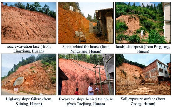
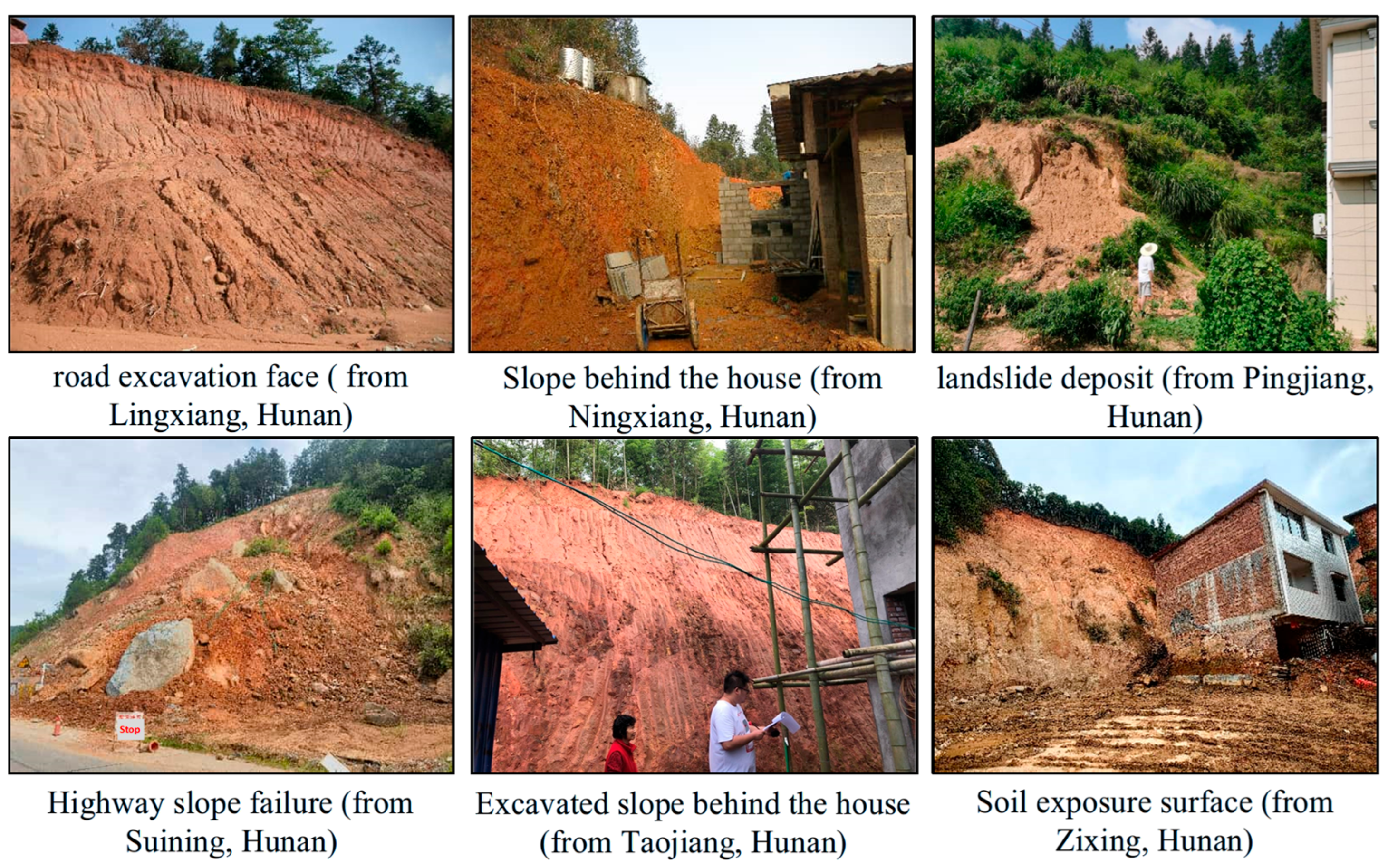
Image data were sourced from field geological surveys and survey sites in 21 counties of Hunan Province, China (Figure 5), captured using digital cameras under natural light conditions. A total of 284 original images were collected, with an average resolution of approximately 3066 × 2359 pixels (ranging from 290 × 290 to 8000 × 6000 pixels). It should be noted that field image collection was not strictly random sampling according to stratum distribution proportions; rather, to ensure sufficient visual samples for each class in model training, the collection density of RNGC outcrops with significant gravelly characteristics was intentionally increased. Therefore, the class distribution of the image dataset does not represent the actual geological distribution proportions.

Figure 5. Examples of field soil image collection.

The original images were segmented into 10,096 image patches using non-overlapping uniform slicing (sliding window step = 256 pixels, window size = 256 × 256). Subsequently, two certified geological engineers with over 5 years of field survey experience independently screened and labeled each patch. Non-soil interference patches (vegetation, tools, gloves, and heavy shadow occlusion) were removed, and Level-1 class labels (RNC/RNSC/RNGC) were assigned based on visual estimation of >2 mm gravel content following the classification scheme in Section 2.2. Discrepant samples were resolved through joint discussion to reach consensus. Finally, 3380 valid pure soil image patches were retained for model training. The sample quantities for the three soil types were 1078 RNC, 1086 RNSC, and 1216 RNGC, with a relatively balanced overall class distribution to meet the model training requirements for multi-class classification under small-sample conditions. In the subsequent dataset partition (train/validation/test), all image patches derived from the same original image were strictly assigned to the same set to circumvent the inflated generalization performance caused by local feature leakage.

To establish an association between image patches and the physical and mechanical indicators of the geotechnical tests in Section 2.3.1, so as to provide statistical attribute anchoring for the soft-label generation of Level-2 classification, this study constructed a two-level geographic matching strategy: L1 matching—Image patches were precisely matched with geotechnical test records from the same county and the same Level-1 classification (RNC/RNSC/RNGC), covering 44.4% of image patches; L2 matching—For image patches that could not be matched at the L1 level, the statistical mean values of physical and mechanical indicators for the same Level-1 classification across the entire province were assigned, covering the remaining 55.6% of image patches. The rationality of this strategy lies in the fact that, although the physical and mechanical indicators of granite residual and slope-wash soils within the same gradation type exhibit regional differences, the statistical central values can still reflect the basic attribute intervals of that soil type, which is sufficient to support the probabilistic allocation of Level-2 classification soft labels. Additionally, the global provincial mean was reserved as the ultimate fallback, which was not triggered in this dataset.

Through the aforementioned matching strategy, 100% geotechnical statistical attribute coverage was ultimately achieved for all 3380 image patches, establishing the data foundation for subsequent generation of Level-2 classification soft labels based on the liquidity index (IL) distribution.

2.4. Image Preprocessing and Data Augmentation

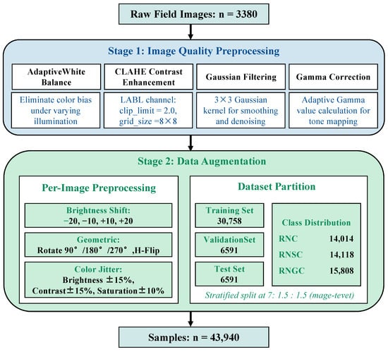
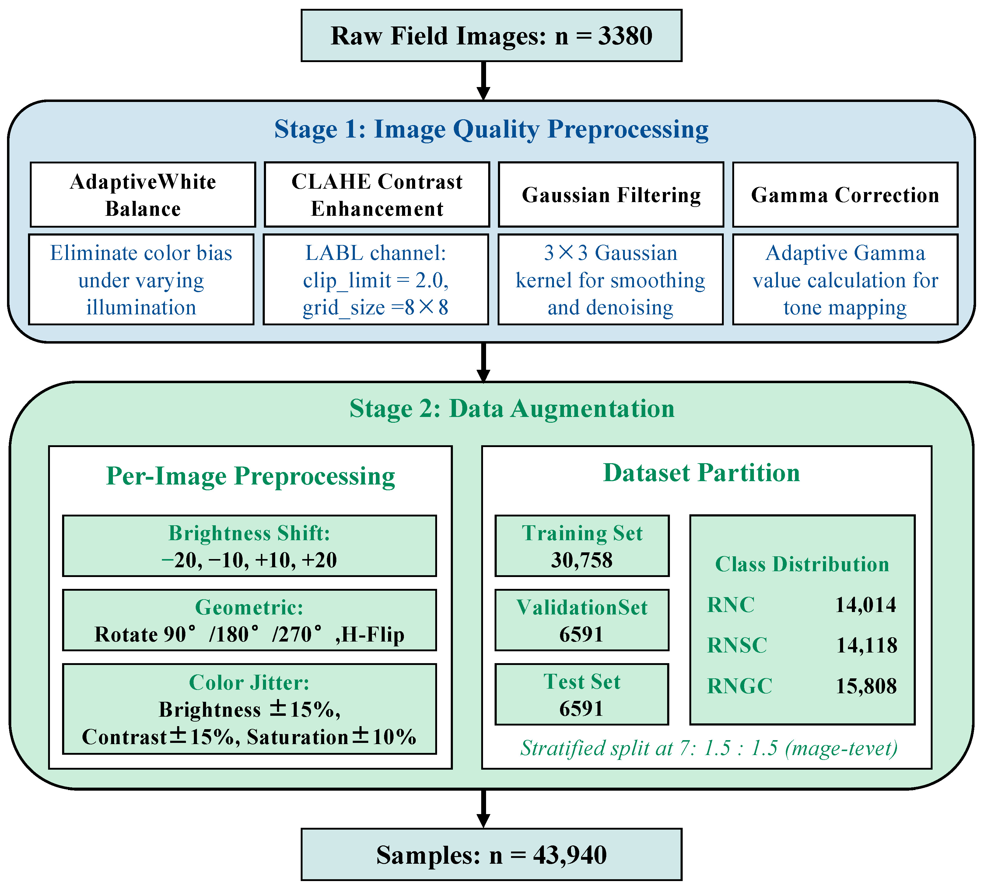
To address the issues of uneven illumination, noticeable color bias, and limited sample size in field images, this study designed an image quality restoration and data scale expansion scheme (Figure 6), comprehensively referencing existing geotechnical image processing methods [7,12,13,21].

Figure 6. Flowchart of two-stage image preprocessing and data augmentation.

The first stage is image quality preprocessing. (1) Adaptive white balance: The Gray World algorithm was employed for color constancy correction to eliminate color biases introduced by different shooting times and illumination conditions [21]. (2) CLAHE contrast enhancement: Contrast-Limited Adaptive Histogram Equalization (clip_limit = 2.0, grid_size = 8 × 8) was applied on the L channel of the LAB color space to enhance local texture details, particularly the contrast at the boundary between coarse and fine particles [12]. (3) Gaussian filtering denoising: A 3 × 3 Gaussian kernel was used for smoothing filtering to suppress high-frequency noise introduced during image acquisition [7]. (4) Gamma correction: The Gamma value was adaptively calculated based on the brightness histogram of each image to normalize the overall brightness, reducing the overall brightness differences caused by different shooting angles and exposure conditions [12]. The selection of the aforementioned enhancement parameter ranges was determined based on pre-statistical analysis of the brightness, contrast, and noise levels of field images, and was verified through small-scale pre-experiments (100 images), confirming that the processed images did not introduce obvious artifacts and that features were completely preserved.

The second stage is data augmentation. To expand the sample size and improve the model’s generalization ability for complex field imaging conditions, 13-fold augmentation was performed on the 3380 preprocessed images (i.e., each image retained the original and additionally generated 12 variants). The specific augmentation strategies included: (1) four brightness shifts: applying offsets of −20, −10, +10, and +20 on the V channel in HSV space to simulate different illumination intensities; (2) seven geometric transformations: combinations of 90°, 180°, 270° rotations and horizontal flip; (3) one color jitter: random perturbation within brightness ± 15%, contrast ± 15%, and saturation ± 10% to simulate camera parameter differences. It should be noted that the three types of augmentation were applied independently and randomly on each image (i.e., only one type of augmentation was applied to a single image), to avoid excessive distortion caused by the superposition of different augmentation methods.

The dataset was partitioned using stratified random sampling at the original-image level in a 7:1.5:1.5 ratio, and this partition was performed before data augmentation: the 284 original images (together with all 3380 patches derived from them) were first assigned to the training, validation, and test groups, and the 13-fold augmentation was subsequently applied within each group, so that every augmented variant remains in the same group as its source image. This procedure guarantees that no patch or augmented variant derived from the same original image is shared between groups, eliminating local feature leakage. After augmentation, a total of 43,940 images were obtained (14,014 RNC, 14,118 RNSC, and 15,808 RNGC), resulting in 30,758 training images, 6591 validation images, and 6591 test images (Table 4). Accordingly, the test set is composed of the 13-fold augmented variants of the 507 held-out original patches (507 × 13 = 6591) rather than solely unmodified observations. This design was adopted because evaluating on only approximately 507 original patches would yield class-wise estimates that are statistically unstable for model comparison, whereas the augmented test variants preserve the photometric and geometric variability representative of field acquisition conditions. We nevertheless acknowledge that the reported metrics thus reflect performance on the augmented image distribution, and an evaluation restricted to entirely unmodified observations would be a useful complementary check in future work.

Table 4. Statistical partition of image dataset.

Dataset	Samples	RNC	RNSC	RNGC
Training	30,758	9672 (31.4%)	10,049 (32.7%)	11,037 (35.9%)
Validation	6591	2093 (31.8%)	2119 (32.2%)	2379 (36.1%)
Test	6591	2249 (34.1%)	1950 (29.6%)	2392 (36.3%)
Total	43,940	14,014 (31.9%)	14,118 (32.1%)	15,808 (36.0%)

To empirically verify the absence of cross-split near-duplicate images, a perceptual hash (pHash) similarity analysis was conducted across all 281 original field photographs (three images were excluded due to file corruption). The pHash algorithm computes a 64-bit hash based on the discrete cosine transform (DCT) of each down-scaled grayscale image, and the Hamming distance between two hashes quantifies their visual dissimilarity. A threshold of Hamming distance ≤ 10 (out of 64 bits) was used to identify near-duplicate image pairs, which is a widely adopted criterion in perceptual near-duplicate detection and is robust to minor resizing, brightness adjustment and slight cropping. The pHash computation was implemented using the Python imagehash library.

Among 39,340 unique image pairs (281 × 280/2), only 3 pairs had a Hamming distance ≤ 10, of which 1 pair spanned different dataset splits: NX-005_RNSC and NX-007_RNSC (both from Ningxiang County, photographed on 24 November 2023, pHash distance = 0, indicating visually identical content). However, this pair was assigned to the validation and training sets, respectively—not to the test set. No near-duplicate original images were shared between the training and test sets. The mean Hamming distance for cross-split pairs (31.28) was comparable to that for within-split pairs (31.38), confirming that the stratified partition effectively prevented visual data leakage at the original-image level.

This empirical verification complements the procedural partitioning rule described above and confirms that the reported test performance is not inflated by near-duplicate image content between the training and test sets.

2.5. Model Evaluation Metrics

The trained model was evaluated on an independent test set (6591 samples). Since the test set was class-balanced during construction to ensure sufficient sample quantities for each class (Section 2.3.2), with similar quantities across classes, this study uses macro-F1 as the primary evaluation metric to equally reflect the model’s recognition ability for each class. Accuracy, per-class precision, and recall are also reported as auxiliary references.

For each class, the One-vs-Rest strategy was used to calculate precision and recall: Precision_i = TP_i/(TP_i + FP_i), Recall_i = TP_i/(TP_i + FN_i), where TP_i, FP_i, and FN_i are the true positives, false positives, and false negatives for class i, respectively.

The F1-score for each class is calculated as: F1_i = 2 × Precision_i × Recall_i/(Precision_i + Recall_i).

$$\mathrm{m}\mathrm{a}\mathrm{c}\mathrm{r}\mathrm{o}-\mathrm{F}1={\displaystyle \frac{1}{\mathrm{C}}}{\displaystyle \sum _{\mathrm{i}=1}^{\mathrm{C}}}\mathrm{F}\mathrm{l}\_\mathrm{i}$$

The $\mathrm{m}\mathrm{a}\mathrm{c}\mathrm{r}\mathrm{o}-\mathrm{F}1$ is defined as the arithmetic mean of F1-scores across all classes, where C = 3 is the total number of classes. The overall accuracy is the ratio of correctly predicted samples to the total number of samples in the test set.

Additionally, a confusion matrix was plotted to visually present the misclassification distribution between classes, with particular attention to the omission rate of the rare class (RNGC) and its confusion patterns with other classes (especially RNSC).

3. Results and Analysis

3.1. Dataset Statistical Characteristics

The geotechnical test dataset comprised 7678 records covering 21 counties in Hunan Province. The classification labeling was completed through the “manual verification + Random Forest automatic inference” strategy: 1023 samples were manually verified and labeled by professional geological personnel in the first stage, of which 869 definitive three-class labels were retained in the final merged dataset after deduplication and quality control (the remaining manually reviewed records were identified as non-soil, non-residual, or ambiguous categories and excluded from the three-class labeling). The Random Forest model was trained on the accumulated verified label set of 6012 samples and automatically assigned labels to 636 additional records meeting the minimum feature-availability criterion, whereas 1030 records with fewer than two available core indicators were retained without three-class labels. The final labeled dataset consisted of 6648 records: 5138 RNC (77.3%), 1354 RNSC (20.4%), and 156 RNGC (2.3%). The data quantity varied significantly across counties, with Ningxiang City having the most at 288 records and Xinning County the fewest at only 1 record, reflecting the spatial non-uniformity of geological survey work intensity in the study area. In terms of feature missing rates, moisture content (5.1%) and plasticity index (7.7%) had relatively low missing rates, while natural density (75.2%) and cohesion (51.8%) had relatively high missing rates, posing certain constraints on subsequent multi-indicator joint analyses (such as feature completeness in Random Forest modeling).

For the image dataset, among the 3380 pure soil image patches, 1078 were RNC (31.9%), 1086 were RNSC (32.1%), and 1216 were RNGC (36.0%), with a relatively balanced distribution across the three classes (maximum difference of approximately 13%), which is conducive to balanced CNN training. Through the two-level geographic matching strategy, all 3380 image patches obtained corresponding geotechnical statistical attributes, with L1 precise matching covering 44.4%, L2 same-class provincial mean covering 55.6%, and L3 global fallback not triggered.

3.2. Model Evolution and Comparison

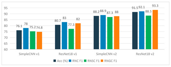
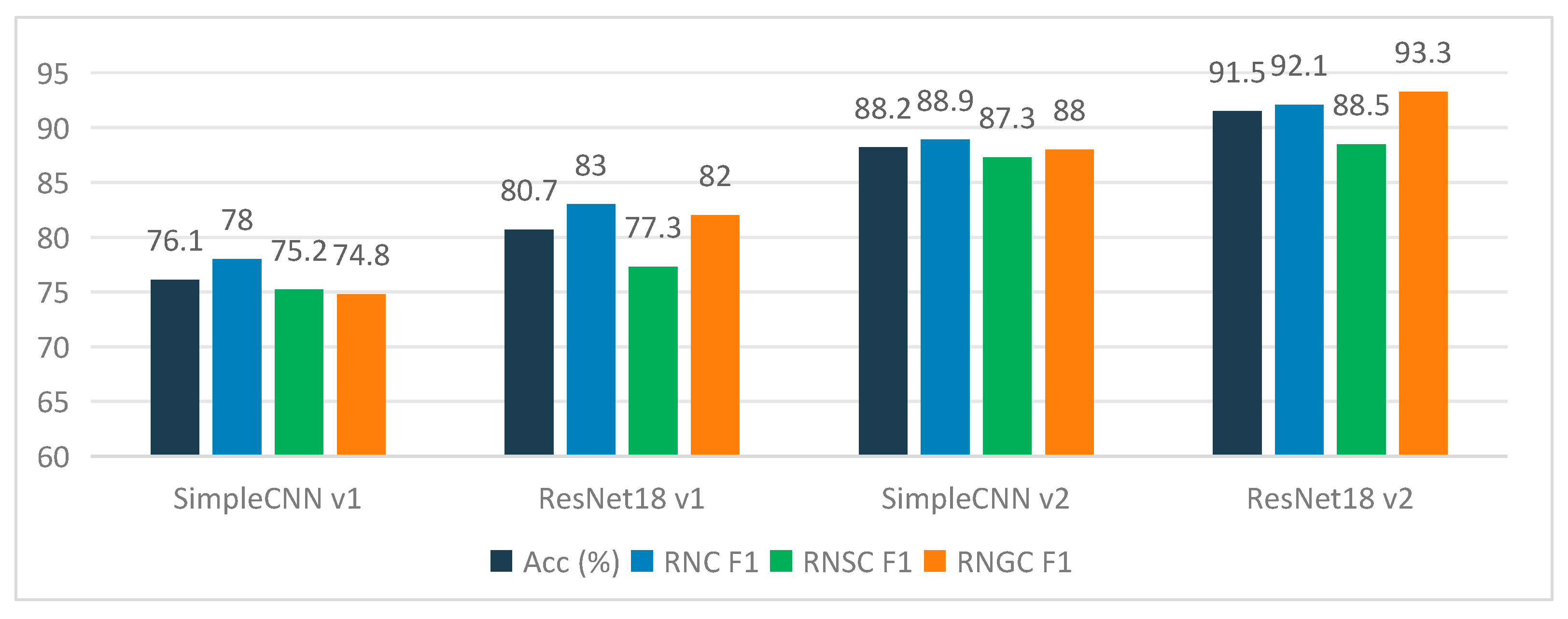
To determine the optimal model architecture, four sets of comparative experiments were conducted under the same dataset conditions (Table 5). Starting from a lightweight LightCNN model with four convolutional layers (SimpleCNN v1) as the baseline, transfer learning (ResNet18 v1), data augmentation (SimpleCNN v2), and the combination of both (ResNet18 v2) were progressively introduced. The experimental results show that transfer learning improved accuracy from 76.13% to 80.67% (+4.54 percentage points), 13-fold data augmentation improved LightCNN accuracy to 88.18% (+12.05 percentage points), and the combination of both (ResNet18 v2) achieved the optimal result of 91.46% with a macro-F1 of 0.9128 (Figure 7). Further analysis revealed that, under the experimental conditions of this study, the accuracy improvement from data augmentation (+12.05 percentage points) was greater than that from transfer learning (+4.54 percentage points). However, it should be noted that the two were measured on different backbone networks (LightCNN vs. ResNet18), and their relative magnitudes only reflect the trends under the experimental settings of this study and should not be over-extrapolated. In particular, the four configurations in Table 5 do not constitute a fully crossed 2 × 2 ablation on a single backbone: the no-transfer-learning baselines were implemented with a lightweight four-layer CNN (SimpleCNN) rather than a randomly initialized ResNet18, so the contrast between SimpleCNN v1 and ResNet18 v1 (+4.54 pp) additionally involves the difference in architectural capacity (0.4 M vs. 11 M parameters), not weight initialization alone.

Table 5. Comparison of Level-1 classification performance of different model versions (Test set).

Model Version	Architecture	Augmentation	Acc (%)	RNC F1	RNSC F1	RNGC F1
SimpleCNN v1	LightCNN (400 K)	×	76.13	0.780	0.752	0.748
ResNet18 v1	ResNet18 (11 M)	×	80.67	0.830	0.773	0.820
SimpleCNN v2	LightCNN (400 K)	13×	88.18	0.889	0.873	0.880
ResNet18 v2	ResNet18 (11 M)	13×	91.46	0.921	0.885	0.933

Figure 7. Comparison of classification performance among different model versions.

The rationale for this ablation design is twofold. First, the objective of Table 5 was to quantify the practical benefit of the adopted engineering strategy—a pre-trained deep backbone combined with systematic augmentation—relative to a from-scratch lightweight alternative that can be trained under the same computational and data constraints, rather than to isolate the pure effect of weight pre-training with all other factors held constant. Notably, a randomly initialized ResNet18 with 11 M parameters would carry a high risk of severe overfitting under the small-sample field image setting, yielding limited engineering reference value compared with a lightweight from-scratch model. Second, the augmentation contribution was measured in an architecture-consistent manner: the +12.05 pp gain from SimpleCNN v1 to SimpleCNN v2 was obtained on the identical LightCNN backbone, and the further +3.28 pp gain from SimpleCNN v2 to ResNet18 v2 reflects the additional benefit of the pre-trained deeper backbone under augmented conditions. The direction of the transfer-learning benefit itself is well established in the soil and geotechnical image classification literature [3,4,9,22]. A same-backbone comparison between the pretrained and randomly initialized ResNet18 under identical optimization settings, which would cleanly isolate the pre-training effect, requires additional training runs under small-sample conditions and is planned as future work; the present results should therefore be read as engineering-level evidence for strategy selection rather than a strict factor decomposition.

3.3. Model Training Process

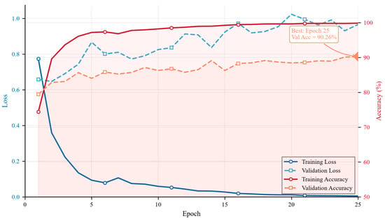
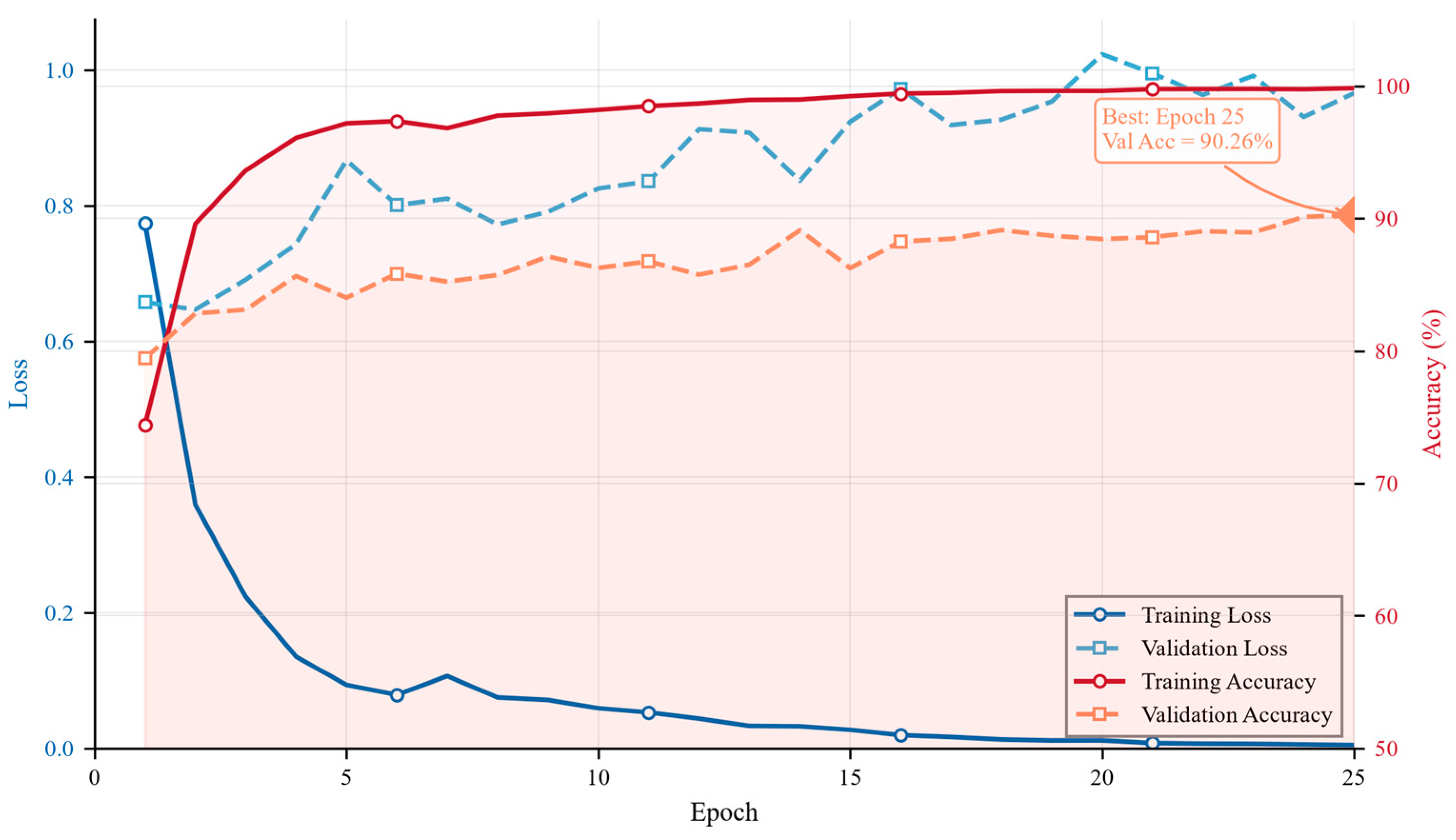
The ResNet18 v2 model completed training on the GTX 1050 Ti (4 GB VRAM) in 25 epochs, with a total time of approximately 6.1 h. As shown in Figure 8, the training loss decreased monotonically from 0.774 in the first epoch to 0.005 in the 25th epoch, with a smooth downward trend. The validation accuracy showed an overall upward trend during training, reaching a maximum of 90.26% in the 25th epoch. The early stopping strategy (patience = 15) was not triggered throughout training, and the validation loss continued to decrease slightly from the 10th to the 25th epoch (from 0.087 to 0.065), indicating that the model had not yet fully converged within this training period, and extending the number of epochs may further improve performance marginally.

Figure 8. Training and validation curves of ResNet18 v2.

3.4. Level-1 Classification Performance

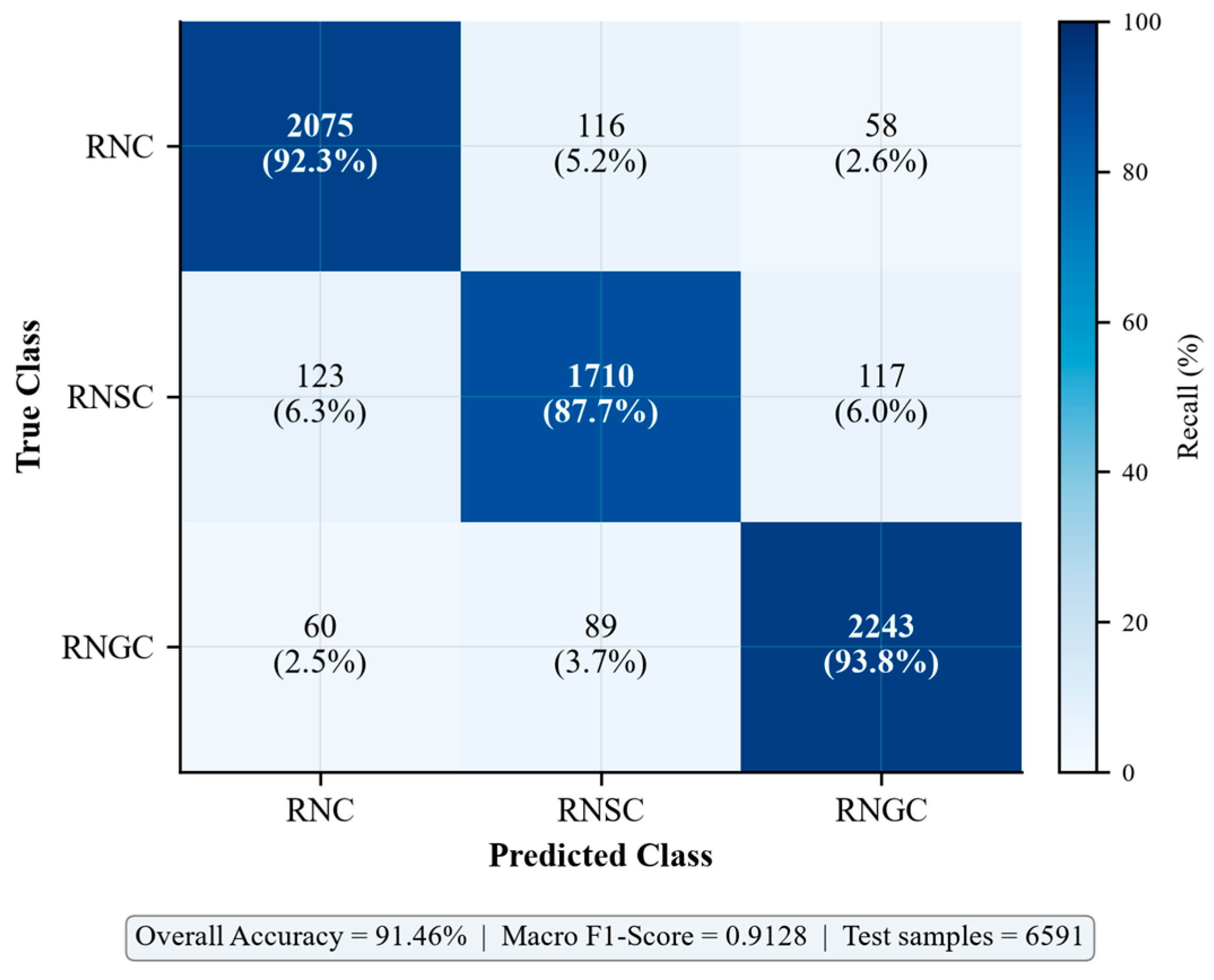
On the independent test set (6591 images), the ResNet18 v2 achieved a Level-1 classification accuracy of 91.46%, a macro-F1 of 0.9128, and a weighted-F1 of 0.9145. The detailed performance metrics for each class are shown in Table 6. The precision for all three classes exceeded 0.89, recall exceeded 0.88, and F1-scores all exceeded 0.88. RNGC (gravelly clay) achieved the highest F1-score (0.933), possibly related to the most visually prominent coarse particle features of this class; RNSC (sandy clay) had the relatively lowest F1-score (0.885), reflecting the greater recognition difficulty caused by its transitional characteristics.

Table 6. Level-1 classification metrics of ResNet18 v2 on the test set.

Class	Precision	Recall	F1-Score	Test Samples
RNC	0.9190	0.9226	0.9208	2249
RNSC	0.8930	0.8769	0.8849	1950
RNGC	0.9276	0.9377	0.9326	2392
Macro avg.	0.9132	0.9124	0.9128	6591

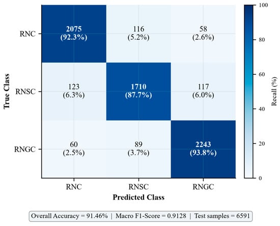
Figure 9 shows the confusion matrix for Level-1 classification on the test set. The main confusion direction for RNC was misclassification as RNSC (116 samples, 5.2%), which is related to both soil types being predominantly fine-grained with similar visual appearance. RNSC exhibited bidirectional misclassification (123 samples misclassified as RNC and 117 as RNGC), reflecting the visual ambiguity of sandy clay as a transitional type. The misclassification between RNGC and RNC (60 samples, 2.5%) was relatively infrequent, indicating that gravelly features have high discriminative power in images.

Figure 9. Confusion matrix for Level-1 classification (ResNet18 v2).

3.5. Model Attention Visualization

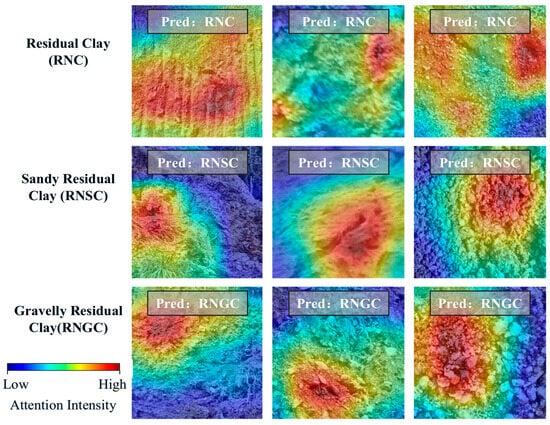
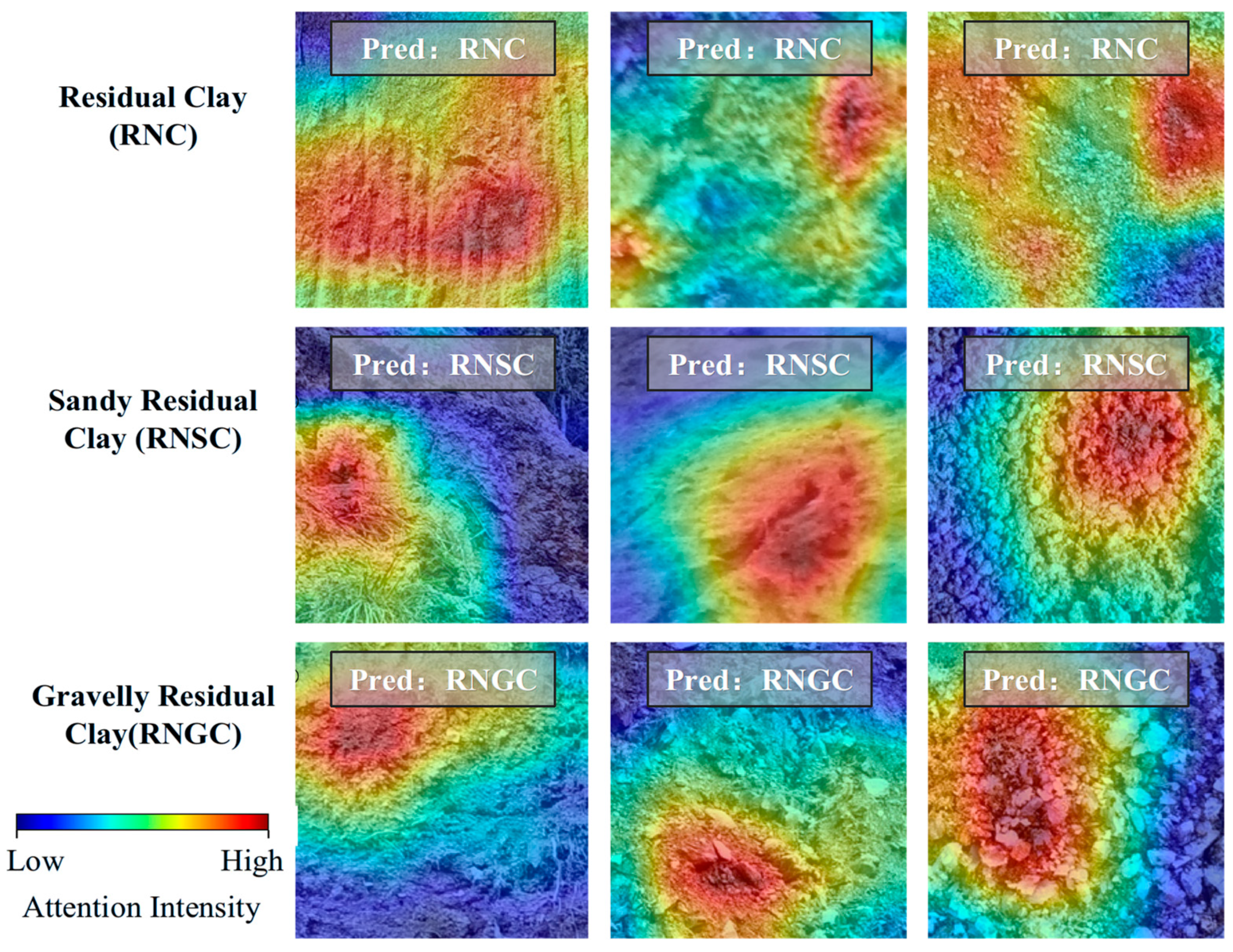
To verify that the model indeed learned the mixed-grain characteristics of granite residual and slope-wash soils rather than relying solely on surface cues such as color or background, Grad-CAM was employed to visualize the decision regions of ResNet18 v2, following interpretability analysis approaches adopted in recent geoscience image classification studies [23]. Figure 10 presents Grad-CAM heatmaps for three samples of each of the three classes, with the heatmap regions indicating the image areas that the model focused on during decision-making.

Figure 10. Visualization of model attention based on Grad-CAM.

As shown in Figure 10, the model’s attention regions highly correspond to the soil particle distribution. In RNC (clay) samples, the heatmap primarily concentrated on areas with fine surface texture and no obvious coarse particles; in RNSC (sandy clay) samples, attention was dispersed across regions with medium-sized particle distribution; in RNGC (gravelly clay) samples, the heatmap clearly concentrated on the locations of coarse gravel particles. This attention distribution pattern is highly consistent with the visual discrimination experience of geological professionals based on particle coarseness, indirectly supporting, from an interpretability perspective, that the model effectively captured visual features related to grain size composition, rather than merely relying on non-essential cues such as illumination, color, or background.

As a caveat on the interpretation of Figure 10, Grad-CAM carries inherent methodological constraints that warrant careful reading. Most directly, the heatmap is upsampled from 7 × 7 feature maps of the final convolutional layer to match the input resolution, giving it relatively coarse spatial granularity that cannot resolve individual soil particles. Beyond spatial resolution, gradient-weighted attention maps capture correlational patterns rather than causal relationships: high activation marks regions that drive the model’s class prediction, but cannot quantify how specific visual features—such as gravel size or packing density—contribute to that decision. More fundamentally, Grad-CAM is a class-discriminative localization tool, not a full feature-attribution method. Techniques including SHAP, integrated gradients, and layer-wise relevance propagation can offer more rigorous pixel-level attribution, but at substantially higher computational cost.

For this work, Grad-CAM was implemented via the open-source pytorch-grad-cam toolbox and selected for its efficiency, native compatibility with ResNet architectures, and prior adoption in geoscience image classification studies [23]. Accordingly, the heatmaps in Figure 10 are treated as qualitative corroboration that the model focuses on geologically meaningful regions, not as definitive proof that the model explicitly encodes grain-size distribution statistics.

3.6. Exploratory Level-2 Classification Results

As an exploratory experiment, this study simultaneously designed a Level-2 classification (plastic state) task based on the liquidity index (IL). On the test set, the Level-2 classification accuracy was 55.95%, with a macro-F1 of only 0.370, where the precision, recall, and F1-score of the soft plastic class were all 0.000, indicating that the model completely failed to recognize the soft plastic state. From the confusion matrix, the prediction results for both hard plastic and plastic classes were concentrated in the hard plastic direction, with zero soft plastic predictions, exhibiting a severe prediction bias.

The fundamental causes can be attributed to two aspects: First, the visual features of the soft plastic state in the visible light band have extremely limited discriminability from hard plastic and plastic states—although moisture content changes affect soil color depth and surface texture, such changes are easily masked by shadows, color bias, and other factors under natural illumination conditions. Second, the Level-2 classification training used soft labels (KL divergence loss), while the evaluation used hard-label accuracy, and the incomplete alignment between training and evaluation objectives may also lead to lower evaluation metrics. This exploratory experiment indicates that effective discrimination of plastic state is difficult to achieve using only visible light images. It is recommended that subsequent studies introduce near-infrared or multispectral imaging to capture spectral features related to moisture content, or employ hyperspectral imaging technology to obtain richer spectral information.

3.7. Sensitivity Analysis Under Imbalanced Class Distribution

As noted by a reviewer, the balanced test set (RNC 34.1%, RNSC 29.6%, RNGC 36.3%) does not reflect the actual class distribution in geotechnical engineering practice, where RNC, RNSC, and RNGC account for approximately 77.3%, 20.4%, and 2.3% of samples, respectively. To provide a more realistic assessment of model performance under deployment conditions, a sensitivity analysis was conducted by resampling the test set according to five different class distributions while preserving the per-class conditional error rates estimated from the original balanced test set.

The conditional probability matrix P(pred|true) was estimated from the original confusion matrix (Table 7), and a new confusion matrix was constructed for each target distribution by scaling the row vectors proportionally to the desired class counts. For the actual distribution, a Monte Carlo simulation with 1000 iterations of multinomial resampling was performed to obtain mean ± standard deviation estimates.

Table 7. Sensitivity analysis of classification performance under different class distributions.

Class Distribution	Accuracy	Macro-F1	Weighted-F1	RNGC F1
Balanced (33/33/33)	0.9123	0.9121	0.9121	0.9267
Actual geo (77.3/20.4/2.3)	0.9135	0.7856	0.9204	0.5613
Moderate (60/30/10)	0.9102	0.8822	0.9117	0.8245
RNC-dominant (90/8/2)	0.9193	0.7426	0.9292	0.5604
RNGC-boosted (50/30/20)	0.9119	0.9050	0.9121	0.8963

Note: For the actual distribution, Monte Carlo simulation (1000 iterations) yielded accuracy = 0.9135 ± 0.003, macro-F1 = 0.786 ± 0.007, weighted-F1 = 0.920 ± 0.003, and RNGC F1 = 0.562 ± 0.018.

Under the actual class distribution, the overall accuracy remained virtually unchanged (91.35% vs. 91.46%), and the weighted-F1 even increased slightly (0.920 vs. 0.915) because the dominant RNC class has the highest precision (0.981). However, the macro-F1 dropped substantially from 0.913 to 0.786, primarily because the precision of the rare class RNGC decreased from 0.928 to 0.401: when RNC constitutes 77.3% of the data, even a small per-class false positive rate (RNC → RNGC: 2.58%, RNSC → RNGC: 6.00%) generates a large number of RNGC false positives relative to the 152 true RNGC samples. The recall of RNGC remained high (0.934), indicating that the model rarely misses true RNGC samples but produces many false alarms in an RNC-dominated environment.

From an engineering deployment perspective, these results suggest that the model can be safely used as a screening tool—in the field, the high recall of the rare class (RNGC) ensures that potentially problematic gravel-rich soils are rarely missed, while the moderate precision (40%) means that approximately 60% of flagged RNGC samples would require confirmatory laboratory testing. For applications where false alarms are costly, class-prior adjustment or threshold tuning at the softmax output level can be applied post hoc without retraining. It should be noted that this sensitivity analysis is based on the assumption that per-class conditional error rates remain constant across class distributions, reflecting the theoretical performance of the trained model under different sampling scenarios. If the model were retrained directly on a naturally imbalanced dataset, class-weighted loss, resampling strategies, or threshold calibration could be further applied to improve rare-class precision, which is outside the scope of the current analysis.

4. Discussion

4.1. Comparison with Existing Methods

Compared with existing domestic and international studies on soil/geotechnical image deep learning classification, this study exhibits the following characteristics.

(1) Data source. Existing studies [3,9,11] mostly used images of laboratory standard specimens or captured under controlled environments, with simple backgrounds and consistent illumination. A notable exception is Zhan et al. [24], who developed an excavated soil classification system combining ResNet18-based soil image deep learning with TDR cone penetration test, achieving 88.7% accuracy on 12 soil types. This study, however, used field in situ images with uneven illumination and complex backgrounds, which are closer to actual engineering scenarios but significantly increase the learning difficulty. Under more challenging conditions, this study achieved an accuracy of 91.46%. Although this is lower than the approximately 95–96% reported in similar studies under laboratory conditions, the gap is primarily attributable to differences in data scenarios rather than insufficient model capability.

(2) Classification target. Existing CNN soil classification studies mostly target 4–7 general soil types (sand/silt/clay or agricultural soil series). This study, for the first time, specifically designed a classification system for the “mixed-grain” characteristics of granite residual and slope-wash soils, possessing stronger regional engineering relevance and application value.

(3) Comparison with ResNet transfer learning methods. Hu et al. [9] achieved 96.10% accuracy on laboratory images of six rock types, higher than the 91.46% of this study. However, the former used standardized photography with inter-class visual differences (granite vs. marble vs. shale) significantly greater than the three types of residual soils in this study (whose differences are mostly gradual changes in fine particle content). Achieving 91.46% under the more challenging field in situ conditions of this study demonstrates the practical potential of ResNet18 in uncontrolled scenarios.

(4) Comparison with ViT-based methods. Zohouri Rad et al. [11] employed a SMOTE-ViT framework to achieve 95.83% accuracy on six standard geotechnical specimens, outperforming the ResNet18 results of this study. However, that method also relied on laboratory standard images and SMOTE oversampling; the generalization performance of ViT in field complex scenarios similar to this study remains to be systematically evaluated, which is also one of the directions for future work.

4.2. Synergistic Effects of Transfer Learning and Data Augmentation

This study systematically compared the effects of transfer learning and data augmentation strategies on classification performance (Table 5). Under the condition of only 3380 original images, transfer learning alone contributed approximately +4.5 percentage points, data augmentation alone contributed approximately +12.1 percentage points, and the combined use of both brought a comprehensive improvement of +15.3 percentage points. The sum of the individual gains of the two strategies was +16.6 percentage points, and the combined gain was slightly lower than the simple sum (by approximately 1.3 percentage points), indicating partial redundancy between the two in feature learning—the texture priors provided by pre-trained weights and the diversified illumination/geometric variations introduced by data augmentation overlap somewhat in the representation space. However, their complementarity remains dominant, and the synergistic effect is overall positive.

The physical explanation for this phenomenon lies in the following: ImageNet pre-trained weights provide general edge, texture, and shape feature priors, enabling the model to possess a good feature extraction foundation from the initial training stage; data augmentation provides diversified input distributions in terms of illumination intensity, shooting angle, and color shift, enabling the pre-trained features to be effectively activated and fine-tuned on a broader domain. This conclusion is consistent with the observations of Jalapur et al. [3] and Pal and Gupta [4] in general soil image classification, as well as the comparative study by Kim et al. [24] on transfer learning models for geotechnical photoelastic image analysis. However, this study found that the gain from data augmentation was approximately 2.7 times that of transfer learning, with a contribution ratio larger than the values reported in the aforementioned literature, indicating that in field image scenarios with sparse samples and high variability, expanding the distribution diversity of training data is more critical than reusing the general feature priors of ImageNet.

4.3. Model Limitations and Future Directions

This study has the following limitations, which also point to directions for future improvement.

(1) Scarcity of RNGC samples in geotechnical test data. In the original geotechnical data, RNGC accounted for only 2.3%. Although class balance compensation was performed during image collection, the training of the Random Forest automatic labeling model was still limited by the scarcity of this class, which may affect the accuracy of some image labels. Future work should specifically supplement field survey and laboratory test data for gravelly clay.

(2) Poor Level-2 classification performance and its implications. The exploratory experiment showed that a single visible light image cannot effectively reflect the plastic state characterized by the liquidity index, because visual changes caused by moisture content (color depth, surface reflectance) are easily masked by interfering factors under natural illumination. It is recommended that subsequent studies introduce near-infrared or short-wave infrared bands, utilizing the spectral absorption features of moisture to assist in plastic state discrimination, as demonstrated by Lim et al. [25] who successfully predicted soil water content using hyperspectral imaging combined with machine learning in landslide-affected areas. or adopt multi-temporal imaging strategies to capture dynamic changes in moisture content.

(3) Deepening interpretability analysis. Grad-CAM analysis in this study confirms that the model focuses on particle-rich regions rather than background cues, but this method only provides coarse spatial localization of gradient-weighted attention and cannot directly confirm that the model has learned explicit grain-size distribution statistics, nor does it establish a causal relationship between highlighted regions and classification decisions. Moving forward, we plan to design targeted ablation experiments to strengthen this verification: occlusion tests that mask gravel-concentrated areas and track prediction probability shifts, grayscale ablation to quantify the contribution of color versus texture features, and head-to-head comparison with feature-attribution XAI methods such as SHAP and layer-wise relevance propagation. For architectures beyond CNNs, Vision Transformers also offer direct inspection of self-attention maps as an additional interpretability pathway.

(4) Image acquisition standardization. The images in this study were sourced from multiple field survey projects, with certain differences in shooting equipment, illumination conditions, shooting distance, and angle. Future work should establish standardized field image acquisition protocols (e.g., fixed shooting distance, inclusion of color cards and scale bars, preference for diffuse light conditions on overcast days) to further reduce data domain variability and improve model stability in practical applications.

(5) Backbone network scalability. This study only employed ResNet18 as the backbone network and has not yet compared it with Vision Transformer (ViT) and CNN-ViT fusion architectures, despite recent studies such as CoreViT [26] demonstrating the superiority of ViT models over traditional CNNs for lithology identification with approximately 97.5% accuracy. Future studies can systematically evaluate the performance of ViT-type models on this dataset and explore hybrid architectures that fuse CNN’s local feature extraction capability with ViT’s global modeling capability. Additionally, advanced data augmentation methods such as Generative Adversarial Networks (GANs) can be used to further mitigate the small-sample problem, as demonstrated by Lu et al. [27] who achieved effective landslide recognition under limited labeled samples using a semi-supervised GAN framework.

(6) Label uncertainty from indirect geotechnical matching. Approximately 55.6% of the image patches (1878/3380) were assigned Level-1 class labels through indirect matching (L2: same classification category across the province), rather than direct correspondence with geotechnical test data from the same county (L1: 44.4%). To quantify the potential impact of this indirect matching on classification performance, a post hoc comparison was conducted on the test set (507 original patches, 6591 augmented images). The L1-matched subset (227 patches) achieved a patch-level accuracy of 91.19%, while the L2-matched subset (280 patches) achieved 93.57%; the difference was not statistically significant (χ² = 0.71, p = 0.399). Within-class error rates were also comparable: for RNC, L1 error rate = 7.09% vs. L2 = 6.52%; for RNSC, L1 = 11.00% vs. L2 = 12.00%. It should be emphasized that the Level-1 classification labels (RNC/RNSC/RNGC) were assigned by geological professionals through visual inspection of the field images and are independent of the geotechnical matching strategy. The indirect matching only affects the Level-2 soft labels (plasticity state statistics), which do not influence Level-1 classification performance. Nevertheless, the potential for label noise from spatial heterogeneity in geological conditions remains a limitation, and future work should prioritize expanding the directly matched (L1) dataset through co-located image sampling and particle-size analysis.

5. Conclusions

This study developed and validated an image recognition framework for the rapid and objective classification of granite residual and slope-wash soils in the mountainous areas of Hunan Province, China. A three-class primary classification scheme (RNC/RNSC/RNGC) anchored on the gravel content of particles larger than 2 mm was established and validated against 7678 geotechnical test records from 21 counties, whose labels were derived through a two-stage strategy combining expert verification with Random Forest inference (five-fold cross-validated macro-F1 = 0.913; out-of-fold agreement with the 869 expert-annotated samples of 94.25%). By pairing 3380 screened field image patches with geotechnical statistics through a two-level geographic matching strategy and applying two-stage image restoration with 13-fold data augmentation, a training corpus of 43,940 images was constructed under small-sample constraints. A ResNet18 model initialized with ImageNet pre-trained weights achieved a Level-1 classification accuracy of 91.46% and a macro-F1 of 0.913 on the independent test set—an improvement of 15.33 percentage points over the baseline without transfer learning or augmentation—with all per-class F1-scores exceeding 0.88, and Grad-CAM visualization confirmed that the model’s attention was concentrated on soil particle distribution regions rather than background cues, supporting the geological plausibility of the learned representations. The ablation results indicated that, under the experimental conditions of this study, data augmentation contributed a larger share of the observed improvement (+12.05 percentage points measured on the same backbone) than the adoption of the deep pre-trained architecture, suggesting that diversifying the illumination and geometric distribution of training data is particularly critical for sparse and highly variable field imagery. Finally, the deployment of the trained model in a lightweight PyQt5 desktop application capable of single-image inference within 0.5 s on consumer-grade hardware demonstrates the practical feasibility of automated and objective soil classification in field geological surveys; future work will focus on multispectral imaging for plastic-state discrimination, standardized field image acquisition protocols, and further interpretability verification through occlusion experiments and same-backbone ablation studies.

References

- Wu, N.S. Study on classification of granite residual soils. Rock Soil Mech. 2006, 27, 2299–2302. [Google Scholar] [CrossRef]
- Pandiri, D.N.K.; Murugan, R.; Goel, T. Smart soil image classification system using lightweight convolutional neural network. Expert Syst. Appl. 2024, 238, 122185. [Google Scholar] [CrossRef] [Scilit]
- Jalapur, S.; Patil, N. An Integrated Deep Learning Framework for Soil Type Classification. SN Comput. Sci. 2025, 6, 251. [Google Scholar] [CrossRef] [Scilit]
- Pal, K.; Gupta, N. Machine learning and deep learning approaches for soil classification: Methods, challenges, and future prospects. Int. J. Remote Sens. 2025, 46, 8488–8545. [Google Scholar] [CrossRef] [Scilit]
- Zhuang, J.R.; Lin, W.; Jian, W.B.; Xia, C.; Huang, Z.H. Study on the microstructure of granite residual soils. Chin. J. Geol. Hazard Control 2025, 36, 136–144. [Google Scholar] [CrossRef]
- Li, Z.S.; Tang, L.S.; Sang, H.T. 3-D micro-structure of the particle and water morphology of the granite residual soil. Acta Sci. Nat. Univ. Sunyatseni 2017, 56, 15–21. [Google Scholar] [CrossRef]
- Yan, B.; Zheng, L.; Wang, X.; Li, Q. Deep learning-based recognition method of red bed soft rock image. Geol. J. 2023, 58, 2418–2426. [Google Scholar] [CrossRef] [Scilit]
- Abdullah, M.A.M.; Mohammed, A.A.; Awad, S.R. RockDNet: Deep Learning Approach for Lithology Classification. Appl. Sci. 2024, 14, 5511. [Google Scholar] [CrossRef] [Scilit]
- Hu, B.; Song, W.D.; Liang, P. Automatic classification method of rock lithology based on ResNet network and deep transfer learning. Bull. Geol. Sci. Technol. 2026, 1–13. [Google Scholar] [CrossRef]
- Li, R.J.; Jiang, X.T.; Lv, Y.H.; Wang, L.B.; Jiang, H.; Zhang, X.T.; Zhang, X.W. Improved densely connected convolutional networks for soil layer classification from cone penetration test data. Rock Soil Mech. 2026, 47, 1096–1109. [Google Scholar] [CrossRef]
- Zohouri Rad, A.; Topal, A.; Tunga, B.; Balkaya, M. A SMOTE–ViT Framework for Advanced Soil Classification on a Self-Generated Geotechnical Image Database. Appl. Sci. 2026, 16, 4063. [Google Scholar] [CrossRef] [Scilit]
- Feng, Z.X. Classification and Intelligent Recognition of Granite Remnant Soil Based on Convolutional Neural Networks. Master’s Thesis, Huazhong University of Science and Technology, Wuhan, China, 2022. [Google Scholar]
- Ma, H.; Han, G.Q.; Peng, L.; Zhu, L.Y.; Shu, J. Rock thin sections identification based on improved squeeze-and- Excitation Networks model. Comput. Geosci. 2021, 152, 104780. [Google Scholar] [CrossRef] [Scilit]
- Chen, X.; Zhang, H.; Wong, C.U.I.; Song, Z. Accelerated Bayesian optimization for CNN+LSTM learning rate tuning via precomputed Gaussian process subspaces in soil analysis. Front. Environ. Sci. 2025, 13, 1633046. [Google Scholar] [CrossRef] [Scilit]
- He, K.; Zhang, X.; Ren, S.; Sun, J. Deep Residual Learning for Image Recognition. In 2016 IEEE Conference on Computer Vision and Pattern Recognition (CVPR); IEEE: Las Vegas, NV, USA, 2016; pp. 770–778. [Google Scholar] [CrossRef] [Scilit]
- Selvaraju, R.R.; Cogswell, M.; Das, A.; Vedantam, R.; Parikh, D.; Batra, D. Grad-CAM: Visual Explanations from Deep Networks via Gradient-Based Localization. In 2017 IEEE International Conference on Computer Vision (ICCV); IEEE: Venice, Italy, 2017; pp. 618–626. [Google Scholar] [CrossRef] [Scilit]
- GB/T 50145-2007; Standard for Engineering Classification of Soil. China Planning Press: Beijing, China, 2008.
- GB 50021-2001; Code for Investigation of Geotechnical Engineering. China Architecture and Building Press: Beijing, China, 2009.
- Liu, C.Y.; Ku, C.Y.; Wu, T.Y.; Ku, Y.C. An Advanced Soil Classification Method Employing the Random Forest Technique in Machine Learning. Appl. Sci. 2024, 14, 7202. [Google Scholar] [CrossRef] [Scilit]
- Chala, A.T.; Ray, R. Assessing the Performance of Machine Learning Algorithms for Soil Classification Using Cone Penetration Test Data. Appl. Sci. 2023, 13, 5758. [Google Scholar] [CrossRef] [Scilit]
- Wu, W.R. Brightness-Controlled Enhancement and Purple Soil Classification. Master’s Thesis, College of Computer and Information Science, Chongqing, China, 2023. [Google Scholar]
- Kim, S.; Nam, B.H.; Jung, Y.-H. Comparison of Deep Transfer Learning Models for the Quantification of Photoelastic Images. Appl. Sci. 2024, 14, 758. [Google Scholar] [CrossRef] [Scilit]
- Dalhat, M.A.; Osman, S.A. Deep learning based identification of rock minerals from un-processed digital microscopic images of undisturbed broken-surfaces. Artif. Intell. Geosci. 2025, 6, 100127. [Google Scholar] [CrossRef] [Scilit]
- Zhan, L.T.; Guo, Q.M.; Chen, Y.M.; Wang, S.Y.; Feng, T.; Bian, Y.; Wu, J.J.; Yin, Z.Y. An efficient classification system for excavated soils using soil image deep learning and TDR cone penetration test. Comput. Geotech. 2023, 155, 105207. [Google Scholar] [CrossRef] [Scilit]
- Lim, H.H.; Cheon, E.; Lee, S.R. Machine learning and hyperspectral imaging to predict soil water content: Methodology and field validation. Earth Sci. Inform. 2025, 18, 109. [Google Scholar] [CrossRef] [Scilit]
- Cao, Z.; Ma, C.; Tang, W.Q.; Zhou, Y.X.; Zhong, H.T.; Ye, S.; Wu, K.Y.; Chen, X.D.; Zheng, D.Y.; Hou, L.; et al. CoreViT: A new vision transformer model for lithology identification in cores. Geoenergy Sci. Eng. 2024, 240, 213012. [Google Scholar] [CrossRef] [Scilit]
- Lu, W.J.; Zhao, Z.A.; Mao, X.; Cheng, Y. An Accurate Recognition Method for Landslides Based on a Semi-Supervised Generative Adversarial Network: A Case Study in Lanzhou City. Appl. Sci. 2024, 14, 5084. [Google Scholar] [CrossRef] [Scilit]
Disclaimer/Publisher’s Note: The statements, opinions and data contained in all publications are solely those of the individual author(s) and contributor(s) and not of MDPI and/or the editor(s). MDPI and/or the editor(s) disclaim responsibility for any injury to people or property resulting from any ideas, methods, instructions or products referred to in the content. |
© 2026 by the authors. Licensee MDPI, Basel, Switzerland. This article is an open access article distributed under the terms and conditions of the Creative Commons Attribution (CC BY) license.