Spatio-Temporal-Frequency Graph Decoupling and Mamba-WKAN Knowledge Distillation for Anomaly Prediction and Early Warning of Power Distribution IoT Devices

Abstract

Power IoT acts as the final frontier of the modern grid, where the reliability of energy supply hinges on precise monitoring. However, current systems often suffer from delayed responses, poor feature separation, and a computational wall when dealing with high-frequency data on the edge. We move past the traditional reactive detection mindset and propose STF-MKD, a framework built on spatio-temporal-frequency graph decoupling and Mamba-WKAN knowledge distillation. Our goal is to shift the operational focus from responding to failures to forecasting them. The first part of the system is the STF-Extractor. It uses dynamic graph attention to map the connections between nodes and a masking game to pull structural features out of the background noise. Following this, we address the wild nonlinear nature of equipment failure with the Mamba-WKAN backbone. By embedding Mexican Hat wavelets and B-splines into the Mamba architecture, the model maintains efficiency while splitting the work: splines track the daily cycles and wavelets lock onto sudden transients. To prevent the model from smoothing away rare anomaly signals, we introduce the TGAR (Teacher-Guided Anomaly-focused Reconstruction) distillation scheme. This one-teacher-two-students setup uses a teacher model with a global view to guide the student predictor. In doing so, the system triggers early warnings based on faint structural shifts before a fault fully develops. Tests on six major datasets, including ETTh/m and WADI, show that STF-MKD outperforms mainstream methods.

1. Introduction

Think of distribution networks as the capillaries of today’s energy internet [1,2,3]. As distributed power sources and electric vehicle charging loads grow, these end segments face increasing operational pressure. The deployment of the distribution IoT (Internet of Things) aims to achieve real-time monitoring of core equipment such as transformers and switch cabinets through a large number of sensors [4].

Most monitoring systems, though, suffer from a noticeable lag. By the time an alarm goes off, the hardware has often already taken irreversible damage. That delay not only drives up repair costs but also puts power supply continuity at risk. Early research in anomaly detection mostly focused on data acquisition and communication architectures. For instance, Luo et al. [5] brought auto-encoders into wireless sensor networks to enable cloud edge collaboration. Later studies explored neighbor monitoring [6] and microservice communication modeling [7]. By structuring systems this way, researchers achieved better data flow, but the underlying logic remained a reactive, passive defense mode. Recently, the focus has shifted toward proactive early warning. Yu et al. [8,9] developed control strategies based on gas electric evolution, while Choi et al. [10] used feedback to link forecasting and detection. These efforts prove that we can identify anomalies early by projecting future states.

The main barrier to accurate early warning is the messy physical nature of grid data. We will find that features in the time, space, and frequency domains are deeply intertwined. Monitoring nodes are bound by physical structure, load curves follow daily rhythms, and high frequency noise constantly washes over the actual fault signals. Early works like Graph Deviation Networks [11] used graph neural networks for spatial dependencies, but they often struggle when loads shift during non-stationary conditions. While the community has moved toward dynamic graphs like Ada-STNet [12] and GLSTGN [13], equipment degradation remains a nonlinear black box. Events like insulation aging or intermittent arcs produce very weak signals that jump nonlinearly before a full breakout. In doing so, even high performance models like iTransformer [14] or PatchTST [15] tend to smooth out these critical precursors due to their global averaging effect. As Karkhaneh et al. [16] and Carratù et al. [17] suggested, failing to dig into time frequency rhythms often means the smallest warning signs stay buried in the background noise.

Warning tasks in the power grid must handle high dimensional data while meeting real time requirements at the edge. Attention-based models are accurate, but they require too much computing power for low spec edge gateways. Selective State Space Models, such as Mamba [18,19], offer a way out with their efficiency and long range modeling. Some recent work, like Fourier-KAN-Mamba [20], tries to combine Mamba with Kolmogorov–Arnold Networks, but these often just stack general operators together. They do not account for the physical constraints of the grid, nor do they fix the problem of smooth predictions caused by sparse anomaly samples. Relying only on mean squared error usually makes the model favor dominant steady states. To focus on rare features when labels are scarce, knowledge distillation offers a path forward. This technique has moved from a simple compression tool [21,22] to a cross task transfer mechanism like AnomalyLLM [23], providing a new lens for sensing sparse signals.

We address these technical bottlenecks with a framework called STF-MKD, short for Spatio-Temporal-Frequency Graph Decoupling and Mamba-KAN Distillation. The core idea is to use the reconstruction error of a Teacher model, which sees the global context, to build an information gradient. This gradient guides the Student model to see potential anomaly trends during the initial observation. The STF-Extractor module uses a masking strategy to make feature representations more robust under an information bottleneck. Such a configuration moves the warning logic from matching past patterns to inferring future states. While foundational concepts like state-space models and knowledge distillation have been explored in general machine learning, existing applications often treat them as black-box operators. The core novelty of STF-MKD lies not in simply stacking these techniques, but in deeply refactoring them with physical-aware priors specifically tailored for power IoT non-stationary anomaly forecasting. By redesigning internal mechanisms, such as splitting KAN bases into wavelets and splines for distinct physical behaviors, and transforming distillation from a compression tool into an anomaly-precursor targeting game, our framework bridges the gap between purely mathematical modeling and real-world electrical engineering requirements. Our work offers the following contributions:

(1)

We propose a spatio-temporal-frequency decoupling mechanism called STF-Extractor. Instead of modeling raw numbers, we use dynamic graph attention to extract physical topology and combine it with a dual view masking strategy. This setup filters out normal daily load swings and pulls hidden structural anomalies out of the noise.

(2)

We built a Mamba-WKAN evolution backbone that fuses wavelets and splines. Unlike existing hybrid models (e.g., standard Fourier-KAN-Mamba) that treat KAN as a generic nonlinear replacement, we innovatively designed a physically interpretable division of labor within the KAN layers: B-splines track the smooth long-term load trends, while Mexican Hat wavelets function as high-frequency sensors to lock onto sudden transient singularities. This redesign grants the backbone the specific reflexes needed to catch sharp nonlinearities of degrading equipment.

(3)

We designed a Teacher-Guided Anomaly-focused Reconstruction distillation framework, i.e., TGAR. Deviating from traditional knowledge distillation aimed at model compression, TGAR introduces a novel asymmetric learning paradigm. We creatively utilize the “reconstruction failure” of an omniscient Teacher as dynamic weights to guide the Student predictor. This paradigm explicitly solves the common “prediction passivation” issue, forcing the model to target faint anomaly precursors rather than smoothing them away into the dominant healthy manifold.

(4)

Extensive tests on six datasets including ETTh/m, SWaT, and WADI show that STF-MKD maintains high linear throughput on the RTX 5090 platform. By achieving a longer warning lead time than SOTA methods, the proposed framework provides a practical path for moving power IoT from reactive fixups to proactive defense.

2. Materials and Methods

2.1. Problem Definition

2.1.1. Multivariate Time Series Representation

Think about a typical power zone. We usually have N sensors placed at critical points—things like oil temperature probes in transformers, partial discharge sensors in switchgears, or current transformers in smart meters. At any given time t, these devices capture a multi-dimensional snapshot of the system. By looking at a history of length L, we can build a high-dimensional tensor that represents the evolution of the equipment. We define this observed history as:

$${\mathcal{X}}_o=\{x_{t-L+1},x_{t-L+2},\dots ,x_t\}\in {ℝ}^{L\times N\times D}$$

(1)

Here, $x_t\in {ℝ}^{N\times D}$ is the state vector for all N nodes at time t. We keep the D dimensions for each node because a single sensor often tracks multiple parameters like amplitude, phase, and frequency simultaneously.

It can be noticed that we keep the spatial boundaries of these N nodes intact during the initial processing. We do this to let the graph module see the actual physical connections between sensors via the adjacency matrix. It is only when we are done decoupling the spatio-temporal features and ready for the Mamba backbone that we flatten the nodes and features into a single sequence channel C = N × D. This keeps our math consistent and prevents the model from getting lost in a dimensionality explosion.

2.1.2. Task Formulation

The main shift we are proposing here is in the task itself. Most researchers try to figure out if the grid is failing right now. But for a system where staying online is everything, a split-second warning is not very useful [24]. We have shifted the focus to how a fault evolves over time. We are essentially turning anomaly detection into an anomaly forecasting and early warning task. Grid failures are notoriously quiet before they happen. Trying to predict the exact second a wire snaps is almost impossible because power systems are chaotic. Instead, we aim to identify high-risk states within a future time window. This gives operators enough time to shed loads or dispatch a repair crew.

Mathematically, this is a hybrid mapping problem. Since we rarely have labeled anomaly data in real-world grids, training a simple classifier is out of the question. We instead built a compound system f that links a predictor sub-network Φ and an evaluator sub-network Γ:

$$f({\mathcal{X}}_o)=Threshold\left(\mathsf{\Gamma }([{\mathcal{X}}_o,\mathsf{\Phi }({\mathcal{X}}_o)])\right)\to \{0,1\}$$

(2)

Our workflow looks like this: Φ takes the history and guesses the future sequence ${\mathcal{X}}_f\in {ℝ}^{T\times C}$. Then, Γ takes the current observation and stitches it together with that predicted future. It looks at this combined trajectory to check if the underlying structure is still healthy. Finally, it outputs a sequence of anomaly scores ${\left\{S_t\right\}}_{t=1}^T$. If the highest score in that future window jumps over our dynamic threshold, i.e., max(S_t) > γ, the system triggers an early warning.

2.1.3. Notation

Table 1 defines the key symbols across the following sections.

Table 1. Key notations in this paper.

Category	Symbol	Domain	Physical Meaning
Dimensions	N, D, C	${\mathbb{Z}}^{+}$	Nodes (N), features (D), and total flattened channels (C = N × N)
	L, T, w	${\mathbb{Z}}^{+}$	History (L), prediction (T), and look-back (w) windows
Signals	${\mathcal{X}}_o$	${ℝ}^{L\times C}$	The current multivariate input history
	$\mathcal{Y}$	${ℝ}^{L\times C}$	Future ground truth (visible only during offline training)
	${\mathcal{X}}_f$	${ℝ}^{L\times C}$	Predicted future trajectory from the Predictor
	$\overline{\mathcal{Y}}$	${ℝ}^{L\times C}$	Reconstructed future signal from the Teacher model
	Zcat	${ℝ}^{(L+T)\times C}$	The concatenated context of history and future
Features	αt,ij	[0, 1]	Dynamic topology attention weights at time t
	${\mathsf{\zeta }}_t$	${ℝ}^{+}$	Temporal fluctuation score reflecting structural stability
	${\pi }_t$	[0, 1]	Masking probability generated for a specific moment
	M	{0, 1}L	Discrete hard mask used for feature decoupling
	${\mathcal{Z}}_{stf}$	${ℝ}^{L\times C}$	Fused spatio-temporal-frequency representation
	${\mathcal{F}}_{eval}$	${ℝ}^{(L+T)\times C}$	Deep latent representation from the Evaluator
Inference	ωij	[0, 1]	Anomaly-focused weights generated by the Teacher
	${\Delta }_{freq}$	${ℝ}^{+}$	Global frequency energy mismatch in a window
	St	${ℝ}^{+}$	Final pre-emptive anomaly score
	$\gamma$	${ℝ}^{+}$	Adaptive warning threshold from the SPOT algorithm
Hyperparams	$\lambda ,\alpha$	${ℝ}^{+}$	Balancing coefficients for losses
	$\rho$	(0, 1)	Information masking budget ratio

2.2. Overall Architecture

Moving from reactive diagnostics to proactive early warning requires a strategy that can handle the messy nature of power IoT data. We have to deal with strong physical coupling between nodes while simultaneously filtering out periodic loads and high-frequency noise that tend to hide early-stage fault signals.

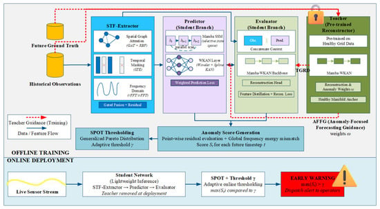
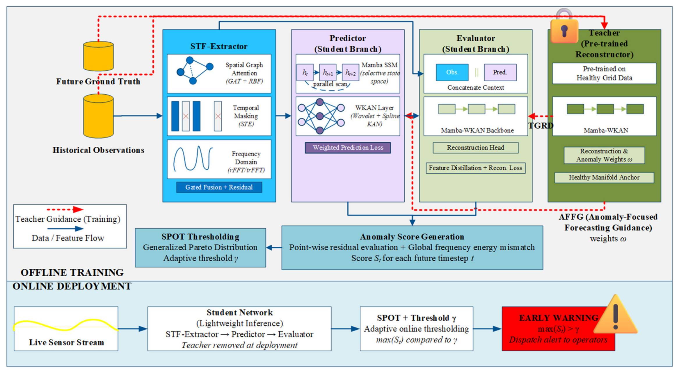
The proposed STF-MKD framework is organized into three progressive modules, each designed to tackle a specific challenge in power grid data, as illustrated in Figure 1. The first stage is the STF-Extractor, which handles feature decoupling and reconstruction. We use a graph network to model the physical structure of the distribution network in the spatial dimension. For the time and frequency domains, we introduce a dual-view dynamic masking mechanism. This setup lets the model automatically filter out periodic load fluctuations and background noise, effectively isolating hidden structural changes.

Figure 1. The overall framework of the proposed STF-MKD.

Next is the Mamba-WKAN Backbone, our engine for long-term temporal reasoning. We opted for a Selective State Space Model (Mamba) because it offers linear time complexity, making it much more suitable for long sequences than a standard Transformer. Power grid faults like intermittent arcs or single-phase grounding have wild nonlinear characteristics. By replacing standard MLPs with KAN layers that fuse wavelets and splines, we give the backbone the sharp reflexes needed to catch these high-frequency transients.

Finally, we have the Teacher-Guided Dual-Branch Distillation layer. Anomalies in the grid are rare, which often tricks prediction models into outputting a smooth, healthy trend that ignores the problem. Our solution is a joint training setup where a Teacher model, which has already learned the healthy grid manifold through self-supervised pre-training, mentors the Student network. The Teacher uses its god-view to generate weights that force the Predictor to look at fault precursors, while distilling its hidden knowledge into the Evaluator to keep the two sub-networks aligned.

During offline training, we feed a combined signal $Z_{cat}=[{\mathcal{X}}_o,\mathcal{Y}]$ into the Teacher. Since the Teacher only knows what a healthy grid looks like, it struggles when it sees a sequence containing actual future anomalies $\mathcal{Y}$. This struggle creates a reconstruction bias, which we turn into anomaly-focused weights ω_ij for specific time steps i and channels j via Anomaly-Focused Forecasting Guidance (AFFG). From here, the Student network pursues two goals.

First, the Predictor takes the history ${\mathcal{X}}_o$ and tries to map out the future trajectory ${\mathcal{X}}_f$. We inject the Teacher’s weights ω_ij directly into the loss function, forcing the model to get better at fitting the exact moments where anomalies are likely to start. Second, we concatenate ${\mathcal{X}}_f$ and ${\mathcal{X}}_o$ together and hand them to the Evaluator. To stop the prediction errors from snowballing, this same context is fed into the frozen Teacher. We enforce a strict alignment between the Evaluator and the Teacher, distilling the deep latent representations for the future T steps via Teacher-Guided Reconstruction Distillation (TGRD). This ensures the Evaluator inherits the constraints of a healthy system, making it much tougher against prediction noise.

Once we move to online deployment, we strip away the heavy Teacher model. The edge gateway only runs the lightweight Student network. As live sensor data ${\mathcal{X}}_o$ streams in, the Predictor generates a future trajectory ${\mathcal{X}}_f$, which is immediately evaluated for structural deviations. By fitting the tail of these scores to a Generalized Pareto Distribution via Streaming Peaks-Over-Threshold (SPOT), we generate a threshold γ that breathes with the current grid conditions. If the future score jumps over this line, the system flags an early warning.

2.3. Spatio-Temporal-Frequency Decoupling Module

Raw sensor streams in the power IoT are a mix of seasonal load shifts and high-frequency noise. A simple amplitude threshold will not cut it because a normal midday load surge might look a lot like an early-stage fault. The STF-Extractor acts as a surgical tool to pull apart the spatial, temporal, and frequency features.

2.3.1. Spatial-Temporal Graph Construction

To stop mean drift in non-stationary sequences from confusing the model, we start with a sliding window normalization on the observation signal ${\mathcal{X}}_o\in {ℝ}^{L\times N\times D}$. For a specific node n and feature d at time t, we standardize the value using local statistics:

$${\widehat{x}}_{t,n,d}={\displaystyle \frac{x_{t,n,d}-{\mu }_{local}}{{\sigma }_{local}+\epsilon }}$$

(3)

We use local means μ_local and standard deviations σ_local to keep the distribution stable for the following steps.

Because power load shifts can cause sensor relationships to drift, we use a Gaussian RBF kernel to measure the nonlinear correlation between nodes. To keep the warning system causal and prevent looking into the future, we calculate the initial weights e_ij using only the data available up to the current moment. We then use a graph attention mechanism to pull out spatial features. This computation happens in parallel across time steps. For any time t ∈ [1, L], the attention weight α_t,ij between node i and j is calculated using a learnable vector $\overrightarrow{a}$:

$${\alpha }_{t,ij}={\displaystyle \frac{\exp \left(\mathrm{LeakyReLU}({\overrightarrow{a}}^T[W{\widehat{x}}_{t,i}||W{\widehat{x}}_{t,j}])\right)}{{\displaystyle {\sum }_{k\in {\mathcal{N}}_i}\exp \left(\mathrm{LeakyReLU}({\overrightarrow{a}}^T[W{\widehat{x}}_{t,i}||W{\widehat{x}}_{t,k}])\right)}}}$$

(4)

The mapping matrix W is shared across all time steps to keep the temporal logic consistent and the parameter count low. This ensures the spatial weights represent the underlying topology rather than just a specific moment in time. The resulting ${\mathcal{X}}_{space}\in {ℝ}^{L\times N\times D}$ maintains the original physical feature dimensions while being aware of the surrounding grid context.

2.3.2. Decoupling via Dual-View Masking

With the spatial features in hand, we use a masking strategy to dig into the temporal and frequency structures. We start by calculating a fluctuation score ζ_t to pinpoint where structural changes are happening. We look back over a window of length w and find the local mean μ_t,n,d and standard deviation σ_t,n,d:

$$\left\{\begin{array}{l}{\mu }_{t,n,d}={\displaystyle \frac{1}{w}}{\displaystyle \sum _{k=t-w+1}^t{\widehat{x}}_{k,n,d}}\\ {\sigma }_{t,n,d}=\sqrt{{\displaystyle \frac{1}{w-1}}{\displaystyle \sum _{k=t-w+1}^t{({\widehat{x}}_{k,n,d}-{\mu }_{t,n,d})}^2}}\end{array}\right.$$

(5)

The overall fluctuation score ζ_t is the sum of the coefficients of variation across all nodes and features:

$${\zeta }_t={\displaystyle \sum _{n=1}^N{\displaystyle \sum _{d=1}^D\frac{{\sigma }_{t,n,d}}{\left|{\mu }_{t,n,d}\right|+\epsilon }}}$$

(6)

Since picking the Top-K indices is a discrete, non-differentiable step that would break backpropagation, we use a Straight-Through Estimator (STE). A lightweight generator Gmask takes ζ and outputs a probability distribution π_t. During the forward pass, we create a hard mask M ∈ {0, 1}^L:

$$M_t=\left\{\begin{array}{l}1,if{\pi }_t\in Top-K({\pi }_1,\dots ,{\pi }_L)\\ 0,otherwise\end{array}\right.$$

(7)

By forcing the model to reconstruct the signal from only the visible parts, we get a temporal representation ${\mathcal{H}}_{time}$ that is sensitive to structural breaks:

$${\mathcal{H}}_{time}=\mathrm{LayerNorm}(\mathrm{ReLU}(\mathrm{Conv}1\mathrm{D}({\mathcal{X}}_{space}\odot (1-M))))$$

(8)

For the frequency view, we reshape ${\mathcal{X}}_{space}$ and run a real Fast Fourier Transform (rFFT) to get the complex spectrum $\mathcal{C}\in {ℂ}^{F\times C}$:

$${\mathcal{C}}_{f,c}={\displaystyle \sum _{t=0}^{L-1}{x}_{t,c}^{space}\cdot \exp \left(-j\frac{2\pi }{L}tf\right)},f=0,\dots ,⌊L/2⌋$$

(9)

We use a quantile function based on the masking ratio ρ_f to set an energy threshold τ. By filtering out low-energy noise, we get a clean spectrum ${\widehat{\mathcal{C}}}_{f,c}={\mathcal{C}}_{f,c}\cdot (1-M_{f,c})$. After an inverse transform (irFFT) and a linear projection, we end up with the frequency-aware feature ${\mathcal{H}}_{freq}$ which captures the underlying grid rhythm $x^{rhythm}$:

$$\left\{\begin{array}{l}{\mathcal{H}}_{freq}=\mathrm{LayerNorm}(\mathrm{ReLU}(x^{rhythm}{W}_{freq}+b_{freq}))\\ s.t.x^{rhythm}=\mathrm{irFFT}({\widehat{\mathcal{C}}}_{f,c})\end{array}\right.$$

(10)

2.3.3. Gated Fusion of Spatio-Temporal-Frequency Feature

Temporal transients and periodic rhythms often operate at different scales, so we apply LayerNorm to both ${\mathcal{H}}_{time}$ and ${\mathcal{H}}_{freq}$ before bringing them together. We feed the concatenated features $H_{concat}=[\mathrm{LayerNorm}({\mathcal{H}}_{time})||\mathrm{LayerNorm}({\mathcal{H}}_{freq})]$ into a gating network to find the dynamic weights $g=Sigmoid(H_{concat}{W}_g+b_g)$.

To prevent information from washing out through too many layers, we use a residual connection. Since the raw input and the latent space have different dimensions, we use a projection matrix W_res to align them:

$${\mathcal{Z}}_{stf}=\mathrm{LayerNorm}(H_{concat}\odot g)W_p+b_p+\mathrm{Reshape}({\mathcal{X}}_o{W}_{res})$$

(11)

This final fused representation ${\mathcal{Z}}_{stf}$ effectively distills the chaotic raw signals into high-level semantics.

2.4. Mamba-WKAN

Predicting failures in a power distribution network is, at its heart, a challenge of modeling how equipment health drifts over long periods. We built the Mamba-WKAN architecture to serve as the unified evolutionary backbone for the entire framework. Both the Teacher and Student models share this core logic, which helps keep their feature manifolds aligned during the distillation process. To make this work on the edge, we had to rethink the underlying operators to balance raw speed with the ability to fit complex, nonlinear patterns.

2.4.1. Mamba Selection Mechanism

When we are dealing with long historical sequences, the model needs to be smart about what it remembers. Most of the data in a power grid is just background hum; we need a filter that ignores that stationary redundancy and locks onto transient distortions. We use Mamba blocks to achieve this through a Selective State Space Model (SSM). Unlike traditional methods, our mapping parameters are not fixed, in contrast, they depend entirely on the current input ${\mathcal{Z}}_{stf,t}\in {ℝ}^C$.

The system uses projection operators to generate a dynamic step size and projection matrices in real time:

$${\Delta }_t=Softplus(Paramete{r}_{\Delta }+Linea{r}_w({\mathcal{Z}}_{stf,t}))$$

(12)

$$B_t=Linea{r}_B({\mathcal{Z}}_{stf,t})$$

(13)

$$C_t=Linea{r}_C({\mathcal{Z}}_{stf,t})$$

(14)

We apply a Zero-Order Hold (ZOH) to turn these continuous equations into discrete steps. The discretized matrices look like this: ${\overline{A}}_t=\exp ({\Delta }_{t}A)$ and ${\overline{B}}_t={({\Delta }_{t}A)}^{-1}(\exp (({\Delta }_{t}A)-I)\cdot {\Delta }_t{B}_t)$. The hidden state h_t then evolves following a recursive path: $h_t={\overline{A}}_t{h}_{t-1}+{\overline{B}}_t{\mathcal{Z}}_{stf,t}$, with the final output being y_t = C_th_t.

The bottleneck here is usually the serial nature of recursion. To fix this, we exploit the associative property of state transitions and use a parallel scanning algorithm. By defining a binary operator $\otimes$, we can abstract the recursion into a format that a GPU can chew through much faster:

$$(h_t,P_t)=(h_{t-1},P_{t-1})\otimes ({\overline{B}}_t{Z}_{stf,t},{\overline{A}}_t)$$

(15)

2.4.2. Nonlinear Enhancement with WKAN Hybrid Bases

Physical degradation in the grid, like a transformer’s insulation slowly failing, rarely happens in a straight line. Traditional MLPs struggle here because their activation functions are static. Inspired by the Kolmogorov–Arnold theorem, we replaced those MLPs with Wavelet-KAN layers. In a KAN, the activation functions are learnable and sit directly on the connections between neurons. For an input vector $x={[x_1,\dots ,x_{C_{in}}]}^T$, the mapping from neuron i to j follows a specific recipe:

$${\varphi }_{i,j}(x)=w_{b}b(x)+w_s\left(spline(x)+{\displaystyle \sum _m{\alpha }_m\phi \left(\frac{x-c_m}{s_m}\right)}\right)$$

(16)

In which, b(x) is a standard SiLU activation that handles the global context. The real innovation lies in the two-part hybrid base. Standard Multi-Layer Perceptrons (MLPs) or generic KANs often struggle with this domain-specific duality because they employ a single, unified activation strategy. First, a B-spline term, spline(x), tracks the smooth, daily load cycles. It uses the Cox-de Boor recursion to ensure the health trajectory stays physically continuous. Second, we layer on a Mexican Hat wavelet, $\phi (u)=(1-u^2)e^{-u^2/2}$. Since this wavelet is effectively the second derivative of a Gaussian, it is incredibly sensitive to the singularities that signal a pending fault. By letting the model learn the scale s_m and center c_m for these wavelets, we can catch subtle anomaly pulses that a standard network would simply smooth away. Our novel combination specifically addresses the physical reality of power grids, effectively creating an operator-level separation between the base operating state and impending fault risks. The output for each neuron is just the sum of these edge functions: $y_j={\displaystyle {\sum }_{i=1}^{C_{in}}{\varphi }_{i,j}(x_i)}$. To keep our residual connections clean, we ensure the input and output widths stay identical (C_in = C_out = C).

2.4.3. Hierarchical Fusion for Multi-Scale Evolution

The backbone ties these pieces together in a layered structure. Because Mamba handles the recursive flow and WKAN handles the point-to-point mapping, the network does not actually care how long the sequence S is. This flexibility is vital because it means the same architecture can handle a short observation window (S = L) and a longer concatenated context (S = L + T) without breaking a sweat.

We feed the features $H^{(0)}\in {ℝ}^{S\times C}$ through N_layer iterations. In each layer, the data first hits the Mamba sub-layer to sort out the timing:

$$H_{mid}^{(l)}=Mamba\left(LayerNorm(H^{(l-1)})\right)+H^{(l-1)}$$

(17)

Then, it moves into the WKAN sub-layer to tackle the high-order physical mappings:

$$H^{(l)}=WKAN\left(LayerNorm(H_{mid}^{(l)})\right)+H_{mid}^{(l)}$$

(18)

Specifically, Mamba effectively answers the question of when something happened, while WKAN figures out how severe the deviation is in physical terms. By the time the data reaches the final linear head, it has been refined into a deep latent representation:

$${\mathcal{F}}_{out}=Linea{r}_{head}\left(LayerNorm(H^{(N_{layer})})\right)\in {ℝ}^{S\times C}$$

(19)

2.5. Teacher-Guided Dual-Branch Distillation Mechanism

Once the STF-Extractor and Mamba-WKAN backbone are ready, we move to the decision-making hub of the STF-MKD framework. As we noted earlier, power grid anomalies are not just rare; they are often buried under heavy load swings. If we let the student model predict the future on its own, it usually takes the easy way out. It fits the dominant, steady-state patterns and ignores the faint markers of a coming fault—a problem we call prediction passivation. We solve this using a joint training setup based on information asymmetry. Unlike traditional knowledge distillation techniques that merely compress large models into smaller ones for deployment efficiency, our approach introduces a novel cross-task paradigm. The idea is simple: we use a Teacher model that has a full view of the actual future to guide a Student network that only sees the past. This setup forces the Student to learn the hidden markers of risk, effectively repurposing the distillation process as a dynamic anomaly-precursor targeting mechanism.

2.5.1. Establishing Teacher Authority and Anomaly-Focused Guidance

The Teacher needs to know exactly what a healthy grid looks like. Before the main training starts, we pre-train it on a steady-state dataset ${\mathcal{X}}_{pure}$. Finding truly clean data in a messy IoT environment is hard, so we use an engineering-grade purification strategy. We first scrub any periods with known faults from the logs. Then, we apply an adaptive quantile filter to clip any outliers that do not fit the physics of the system. This ensures the Teacher learns the core physical manifold of a healthy grid. Importantly, in real-world IoT deployments where raw historical logs may harbor undetected micro-anomalies (e.g., minor harmonic noise or sensor drift), our framework provides dual-layer immunity. Beyond the adaptive quantile filtering, the B-splines in the WKAN backbone naturally enforce structural continuity and smooth over localized high-frequency micro-distortions during reconstruction, effectively preventing the Teacher from memorizing undetected micro-anomalies as normal grid behavior.

During this pre-training, the goal is to minimize the gap between the input and the reconstruction:

$${\mathcal{L}}_{pre}={\displaystyle \frac{1}{L\times C}}{‖{\mathcal{X}}_{pure}-{\overline{\mathcal{X}}}_{pure}‖}^2$$

(20)

Once this is done, we freeze the Teacher parameters θ_T.

In the main training phase, the Teacher looks at the combined history and future $Z_{cat}=[{\mathcal{X}}_o,\mathcal{Y}]$. Because the Teacher only knows healthy data, it will fail to reconstruct any future signals $\mathcal{Y}$ that contain fault precursors. We take this failure and turn it into a weight ω_ij:

$${\omega }_{ij}={\displaystyle \frac{\exp ({({\mathcal{Y}}_{ij}-{\overline{\mathcal{Y}}}_{ij})}^2)}{{\displaystyle {\sum }_{k=1}^T\exp ({({\mathcal{Y}}_{kj}-{\overline{\mathcal{Y}}}_{kj})}^2)}}}$$

(21)

This ω_ij tells the Student how likely a specific time step i and channel j is to be an anomaly. We then use this to weight the Predictor’s loss:

$${\mathcal{L}}_{\mathrm{Pred}}={\displaystyle \frac{1}{T\times C}}{\displaystyle \sum _{i=1}^T{\displaystyle \sum _{j=1}^C{\omega }_{ij}{({\mathcal{Y}}_{ij}-{\mathcal{X}}_{f,ij})}^2}}$$

(22)

By focusing the Predictor’s attention on high-risk moments, we make the whole system much more sensitive to those quiet, early signs of trouble.

2.5.2. Teacher-Guided Reconstruction Distillation (TGRD)

When we move to online warning, the Evaluator receives a sequence $Z_{cat}^{pred}=[{\mathcal{X}}_o,{\mathcal{X}}_f]$ that already contains some prediction noise. To stop this noise from causing a false alarm, we use the Teacher as an anchor. The Evaluator Γ uses the Mamba-WKAN backbone Ψ with parameters θ_E and a reconstruction head Ψ_head.

We compare the hidden features of the Teacher and the Evaluator:

(1) Teacher Path: Generates stable features from the frozen parameters:

$${\mathcal{F}}_{teacher}={\mathsf{\Psi }}_{{\theta }_T}(Z_{cat}^{pred})\in {ℝ}^{(L+T)\times C}$$

(23)

(2) Evaluator Path: Generates features influenced by the Predictor:

$${\mathcal{F}}_{eval}={\mathsf{\Psi }}_{{\theta }_E}(Z_{cat}^{pred})\in {ℝ}^{(L+T)\times C}$$

(24)

We do not want the history to distract us here. We slice the features to focus only on the future T steps and enforce a hard alignment:

$${\mathcal{L}}_{Distill}={\displaystyle \frac{1}{T\times C}}{‖{\mathcal{F}}_{teacher}[-T:]-{\mathcal{F}}_{eval}[-T:]‖}_F^2$$

(25)

Using the Frobenius norm ${‖\cdot ‖}_F$ here ensures the Evaluator captures the same deep patterns as the Teacher. At the same time, the Evaluator must be able to map these latent variables back to the physical world. The reconstruction head Ψ_head generates a waveform ${\widehat{Z}}_{cat}^{pred}={\mathsf{\Psi }}_{head}({\mathcal{F}}_{eval})$, leading to our reconstruction loss:

$${\mathcal{L}}_{\mathrm{Recon}}={\displaystyle \frac{1}{(L+T)\times C}}{‖Z_{cat}^{pred}-{\widehat{Z}}_{cat}^{pred}‖}_F^2$$

(26)

2.5.3. Structure-Aware Warning Score Generation

By the time training is finished, the Evaluator is essentially a highly specialized checker for the grid normal. When we generate the anomaly scores ${\left\{S_t\right\}}_{t=1}^T$, we have to balance quick transients with global rhythm. The problem with frequency transforms like rFFT is that they lose time resolution. We cannot just line up a frequency residual with a specific second in time.

We solve this with a point-window collaborative approach. We first grab the future reconstructed slice ${\widehat{\mathcal{X}}}_f={\widehat{Z}}_{cat}^{pred}[-T:]$. Then, we calculate a global frequency energy mismatch Δ_freq:

$${\Delta }_{freq}={\displaystyle \frac{1}{F\times C}}{\displaystyle \sum _{f=0}^{F-1}{\displaystyle \sum _{c=1}^C{‖rFFT{({\mathcal{X}}_f)}_{f,c}-rFFT{({\widehat{\mathcal{X}}}_f)}_{f,c}‖}^2}}$$

(27)

This term measures how much the predicted future violates the periodic laws of the grid.

For each moment t ∈ [1, T], we find the final score S_t:

$$S_t={‖{\mathcal{X}}_{f,t}-{\widehat{\mathcal{X}}}_{f,t}‖}^2+{\lambda }_f\cdot Norm({\Delta }_{freq})$$

(28)

We use two defensive strategies in this formula. First, the Norm() function standardizes the frequency term using statistics from the training set, so it does not drown out the time-domain spikes. Second, we use that scalar frequency term to lift the baseline of the whole window. Imagine a hidden fault like a slight harmonic distortion. It might not look like a huge spike at any single point, but it messes up the whole rhythm. By lifting the baseline, we pre-heat the risk level. This allows the anomaly score to cross the dynamic threshold earlier, giving the system the forewarning it needs before a full collapse happens. Adjusting λ_f lets us balance these quick reflexes with long-term oversight.

2.6. Joint Optimization and Training

2.6.1. Multi-Task Joint Loss Function

Getting the STF-Extractor and the Teacher-Student network to work together without fighting is a delicate balance. If we just added the losses together without thinking, the model would likely hit a local minimum or the masking strategy would fail entirely. We built a joint loss function ${\mathcal{L}}_{total}$ to stop that from happening:

$${\mathcal{L}}_{total}={\mathcal{L}}_{\mathrm{Pr}ed}+{\lambda }_{\mathrm{Re}c}{\mathcal{L}}_{\mathrm{Re}con}+{\lambda }_{Dis}{\mathcal{L}}_{Distill}+{\lambda }_M{\mathcal{L}}_{Mask}$$

(29)

where

${\mathcal{L}}_{\mathrm{Pr}ed}$ (Weighted Prediction Loss): Forces the predictor to stare directly at the high-risk periods flagged by the Teacher.

${\mathcal{L}}_{\mathrm{Re}con}$ (Structural Reconstruction Loss): Trains the evaluator to keep its ability to reconstruct signals clean, even when the input is messy with prediction noise.

${\mathcal{L}}_{Distill}$ (Feature Distillation Loss): Passes the Teacher’s noise-resistant habits down to the Evaluator.

Here, we anchor the primary prediction loss weight at λ_Pred = 1.0 as a baseline reference scale, allowing the auxiliary balancing coefficients (λ_Rec, λ_Dis, λ_M) to calibrate representation learning, manifold distillation, and dynamic masking constraints without scale mismatch.

The fourth piece is ${\mathcal{L}}_{Mask}$, our sparsity constraint. Without it, the mask generator would quickly figure out the easiest way to play the game—either by hiding the whole sequence (so the network reconstructs zero) or hiding nothing at all. We use an L₁ norm penalty here to keep things honest. It applies pressure directly to the gap between the probability π_t and our target ratio ρ:

$${\mathcal{L}}_{Mask}={\alpha }_{dc}\cdot {\displaystyle \frac{1}{L}}{\displaystyle \sum _{t=1}^L\left|{\pi }_t-\rho \right|}$$

(30)

in which, we usually set ρ to 0.1. By keeping the generator within this tight information budget, we force it to look for only the most vulnerable spots in the sequence.

2.6.2. Bi-Level Iterative Optimization

Within this framework, the generator is constantly trying to search for and hide the weakest, hardest-to-reconstruct parts of the sequence. Meanwhile, the main network has to learn to reconstruct the signal under this pressure. Algorithm 1 shows this training loop.

Algorithm 1: STF-MKD Bi-Level Optimization

Input: Training set $\mathcal{X}$, pre-trained parameters θT, learning rates η1, η2

Procedure:

1. Initialize θmain, θmask;

2. for each training epoch do:

3.     Step A: Update the main network

4.           Sample batch data ${\mathcal{X}}_{\mathrm{o}}$, $\mathcal{Y}$;

5.           Freeze θmask, run forward pass to get STE hard mask M;

6.           Calculate the total loss ${\mathcal{L}}_{total}$;

7.           ${\theta }_{main}\leftarrow {\theta }_{main}-{\eta }_1{\nabla }_{{\theta }_{main}}{\mathcal{L}}_{total}$ (This updates all parameters in both $\mathsf{\Psi }$ and $\mathsf{\Gamma }$);

8.     Step B: Update the mask generator

9.           Freeze θmain;

10.         Use the STE gradient path to find the loss gradient with respect to $\pi$;

11.         ${\theta }_{mask}\leftarrow {\theta }_{mask}-{\eta }_2{\nabla }_{{\theta }_{mask}}{\mathcal{L}}_{total}$;

12. End for

13. Return θmain;

Output: Trained parameters θmain, θmask

2.6.3. Adaptive Thresholding via SPOT

Once we push the model out to the edge gateways at a substation, we hit a practical wall. Grid noise changes constantly depending on consumer loads. If we use a fixed threshold, a busy period like dinner time will flood the control room with false alarms simply because the background variance went up.

We brought in Streaming Peaks-Over-Threshold (SPOT) to make the alarming logic smarter. Instead of trying to model the whole data distribution—which is a losing game in a non-stationary environment—SPOT only looks at the tail of the anomaly score stream ${\left\{S_t\right\}}_{t=1}^T$.

We assume that any score jumping over an initial baseline u follows a Generalized Pareto Distribution (GPD):

$$F(x)=P(S-u\le x|S>u)=1-{\left(1+{\displaystyle \frac{\xi x}{\beta }}\right)}^{-1/\xi }$$

(31)

where ξ and β are the shape and scale parameters. The system continuously watches the residuals through a sliding window and updates these parameters on the fly. We will notice that the final warning threshold γ adapts automatically:

$$r=u+{\displaystyle \frac{\xi }{\beta }}\left({({\displaystyle \frac{qn}{N_u}})}^{-\xi }-1\right)$$

(32)

in which, n represents the total sample size, and N_u denotes the number of samples that exceed the benchmark u. We set the risk tolerance q very low, i.e., 10⁻⁴, to match what grid operators can tolerate. When the grid hits a peak period, γ rises naturally to swallow the extra noise. But when a true failure starts to form and the structure breaks, the score will punch through this dynamic line in a matter of seconds. This gives us a highly reliable early warning system that operates without human intervention.

3. Results

3.1. Experiment Settings

3.1.1. Dataset

Table 2 provides the specific details of the six benchmark datasets used in our evaluation, including sample size, feature dimensionality, and the anomaly ratio that defines the difficulty of the warning task.

Table 2. Dataset statistics.

Dataset	Domain	Frequency	Total Samples	Dimensions	Anomaly Rate/Events
ETTh1	Power IoT (Transformer)	1 h	17,420	7	Synthetic
ETTh2	Power IoT (Transformer)	1 h	17,420	7	Synthetic
ETTm1	Power IoT (Transformer)	15 min	69,680	7	Synthetic
ETTm2	Power IoT (Transformer)	15 min	69,680	7	Synthetic
SWaT	Industrial CPS (Water)	1 s	944,919	51	11.98%/41 attacks
WADI	Industrial CPS (Water)	1 s	1,221,600	127	5.99%/15 attacks

Our primary verification environment relies on the Electricity Transformer Temperature (ETT) series [25]. This collection tracks two years of operational data from two distinct Chinese power stations, focusing on top-level oil temperature alongside six load-related variables. Because the ETT datasets lack native binary labels, we implement a synthesis strategy based on power system physics to evaluate early warning performance. We use two injection modes. For transient shocks like short circuits, we add white noise with a standard deviation 3 to 5 times larger than the local norm, lasting for 1 to 3 steps. For gradual drifts like insulation aging, we apply an amplitude shift of 1.5 to 2 times the original signal over a window capped at min(T/2, 48) steps. These synthetic anomalies are injected into roughly 4.5% of the test set time steps, mirroring the scarcity of actual fault samples in real distribution networks while providing a controllable baseline for equipment degradation monitoring.

To ensure the realism of this process, the parameters for transient shocks and gradual drifts are directly grounded in electrical power system physics, specifically modeling short-circuit surge currents, switching arcs, transformer oil thermal inertia, and insulation dielectric breakdown, respectively. Furthermore, to eliminate the risk of inadvertently tuning the model to the synthetic injection rules, STF-MKD operates in a completely unsupervised paradigm where training relies solely on purified healthy baseline data, meaning the network never observes or fits synthetic anomaly patterns during training. As a second safeguard against synthetic rule overfitting, and to evaluate how the model scales with high-dimensional sensor coupling, we also evaluate STF-MKD on SWaT [26] and WADI [27]. These real-world industrial CPS testbeds contain authentic, unmodeled physical attack sequences. While these datasets originate from water treatment systems, their closed-loop control logic and dependencies are structurally similar to power distribution grids. SWaT covers over fifty variables under various attacks, resulting in an anomaly rate of 11.98% in the test set. WADI is even more complex, with 127 features and over 1.2 million samples, though its anomaly rate is much lower at 5.99%. Dealing with such imbalanced distributions is difficult because faint anomaly signals are easily buried in the noise of normal operations.

Standardization is a requirement before the data hits the core network. We use Z-score normalization to map all sensor features to a distribution with a zero mean and unit variance. We then slice the sequences using a sliding window. Following our problem definition, each window is split into a historical observation segment L and a future segment T, creating the aligned pairs needed for teacher-guided distillation. Lastly, we do not shuffle randomly in our splitting strategy. Instead, we use the first 70% of each dataset for training, the next 10% for validation, and the last 20% for testing. To meet the Teacher model’s requirement for a pure physical manifold ${\mathcal{X}}_{pure}$, we apply a Z-score threshold to the training set to clip any points exceeding 3σ. This purification process ensures the Teacher learns from a steady-state knowledge source, preventing the Evaluator from inheriting contaminated patterns during the distillation phase.

3.1.2. Baseline Algorithms

We selected seven state-of-the-art algorithms to serve as a benchmark for the STF-MKD framework.

Specifically, Fourier-KAN-Mamba [20] is a hybrid architecture that also combines Mamba state-space equations with Kolmogorov–Arnold Networks and uses a Fourier layer for multi-scale frequency extraction. Comparing our work to this model helps determine if our spatial graph decoupling and teacher–student distillation provide a significant performance boost over a similar operator stack. MambaAD [28] serves as a strong benchmark for IoT anomaly detection, using patch-based tokenization and multi-view extraction to handle long-sequence dependencies efficiently.

In the Transformer domain, iTransformer [14] is a key baseline because it uses inverted attention to bypass the limitations of traditional point-wise modeling, making it excellent for multi-variable forecasting. PatchTST [15] is another outstanding method that relies on channel independence and patching to maintain stability in long-term tasks. For general anomaly detection, Anomaly Transformer [29] and its association discrepancy mechanism remain a standard reference point for measuring how much warning technology has evolved over the last years.

In addition, we also included models with distinct structural approaches. ModernTCN [30] represents the peak of pure convolutional networks in this field, using modern large-kernel structures to balance receptive fields with computational speed. TimesNet [31] takes a frequency-heavy approach by using the Fast Fourier Transform to wrap 1D signals into 2D tensors for variation modeling.

3.1.3. Evaluation Metric

For basic accuracy, we stick with the classic trio: precision, recall, and F1 score. Precision is especially important—it tells us what fraction of alarms actually point to real faults, which helps keep operators from getting so tired of false alarms that they start ignoring the system. Recall measures how many actual events we caught, a critical number in power grids where a single missed fault can lead to a destroyed transformer. In datasets like WADI where anomalies are extremely sparse, reaching only 5.99 percent, we find that pushing for high recall often causes precision to crash. Therefore, we use the F1 score as a balanced measure of overall stability.

Many recent papers in the anomaly detection field use a point adjust strategy to inflate F1-scores [32,33,34]. Under that rule, a model only needs to hit one point in a long anomaly segment to get credit for the entire duration. We believe this masks how slow a model might be to react, which defeats the purpose of early warning. In our experiments, we use raw point-wise or non-overlapping window-wise alignment. A true positive only counts if the model triggers an alarm before or exactly when the physical state changes. The definitions for our statistical metrics are:

$$\mathrm{Precision}={\displaystyle \frac{TP}{TP+FP}}$$

(33)

$$\mathrm{Recall}={\displaystyle \frac{TP}{TP+FN}}$$

(34)

$$\mathrm{F}1\text{-}\mathrm{Score}={\displaystyle \frac{2\times \mathrm{Precision}\times \mathrm{Recall}}{\mathrm{Precision}+\mathrm{Recall}}}$$

(35)

In these equations, TP is the count of correct warnings without using point adjust, while FP and FN represent false alarms and missed detections. We also use the area under the receiver operating characteristic curve to see how the model behaves across different sensitivity levels. This gives us a view of the model’s inherent ability to distinguish between normal operation and a developing fault without being tied to a single threshold.

The most important part of our evaluation is the warning lead time. In a real substation, we care about how much time we buy for the crew to react. We define this metric as the time difference between the first moment the pre-emptive anomaly score S_t stays above the adaptive threshold γ and the actual onset of the fault:

$$\mathrm{WLT}=t_{actual\_fault}-t_{first\_warning}$$

(36)

Because STF-MKD is built for forecasting, t_{first_warning} refers to the actual time the system issues a warning based on its look at the future trajectory. This metric changes the evaluation logic from reactive checking to proactive monitoring. By comparing this lead time across different models, we can show exactly how much room the proposed method provides for emergency response.

3.1.4. Configuration

We ran our experiments on a single NVIDIA GeForce RTX 5090 GPU, which comes with 32 GB of GDDR7 memory and the latest Tensor Cores. We chose this setup because it handles the massive data throughput needed for sequences as long as L = 4096, and it mirrors the kind of hardware being deployed in modern edge gateways or control centers. We also added an Intel Core i9-14900K processor and 128 GB of DDR5 RAM, just to make sure the Mamba architecture can reach its full potential during testing.

On the software, STF-MKD is built on PyTorch 2.3.1 and Python 3.10. We utilized PyTorch Geometric for building the spatial graphs and used the native complex tensor modules in PyTorch for the fast Fourier transform steps to ensure no precision was lost during decoupling.

We set the historical window L to either 192 or 384 steps depending on the sampling frequency of the dataset. For the prediction window T, we tested lengths of 48, 96, and 192 to see how the lead time changes. During training we used a stride of 1 to give the model as much data as possible, but for the test set we switched to non-overlapping windows that way we keep our performance metrics honest.

In the STF-Extractor, we initialized the Gaussian kernel bandwidth η at 0.5. For the dynamic topology, we set the number of neighbors K to 3 for the ETT series and 15 for the more complex WADI dataset. The temporal masking window w was 24, and we fixed the frequency masking ratio ρ_f at 0.15. We also set a sparsity budget ρ of 0.1 for the mask generator to stop it from hiding too much information. The Mamba-WKAN backbone has three layers with a hidden dimension of 256. Thanks to the 5090’s 32 GB of memory, we could keep batch sizes between 64 and 128.

Training is done in two stages. The teacher pre-training uses a learning rate of 1 × 10⁻⁴ on the clean dataset ${\mathcal{X}}_{pure}$ for 20 epochs before we freeze it. The main training phase then follows with the AdamW optimizer. To keep the bi-level optimization stable, we used two separate learning rates: η₁ = 1 × 10⁻⁴ for the main networks and a slower η₂ = 5 × 10⁻⁵ for the mask generation path. Both rates follow a cosine annealing schedule with a weight decay of 1 × 10⁻⁵. We tuned the loss balancing coefficients λ_Rec, λ_Dis, and λ_M to 0.8, 1.2, and 0.1. We also set the frequency bias coefficient λ_f to 0.5 for the final scoring. Main training was limited to 50 epochs with early stopping triggered after 5 epochs of no improvement. Finally, we set the SPOT risk tolerance q to 10⁻⁴ to keep false alarms under control. All results reported here are the average of five independent runs to ensure the numbers are statistically reliable.

3.2. Ablation Analysis

In this section, we designed a set of ablation tests to watch how the F1 score and WLT decayed as we stripped away core modules. We focused our analysis on ETTm1, which has high-frequency power data, and WADI, a complex system with 127 variables. We used the full STF-MKD framework as the upper performance bound and built four variants to test our theories. The first variant, w/o STF, removes the graph topology and time-frequency masking to see how much background noise interferes with the Mamba backbone. The second, w/o WKAN, swaps our nonlinear wavelet layers for standard MLPs. The third, w/o Teacher-Guided mechanism (TGAR), is the most drastic change. We removed the pre-trained Teacher and the distillation paths, forcing the Predictor and Evaluator to train blindly on raw mean squared error. Finally, w/o SPOT replaces our adaptive threshold with a fixed 99th percentile cutoff. Table 3 summarizes these changes.

Table 3. Ablation study results (prediction window T = 96). ↓ represents the decrease value compared to the complete STF-MKD.

Variant	ETTm1			WADI
	F1-Score	AUC-ROC	WLT (Steps)	F1-Score	AUC-ROC	WLT (Steps)
STF-MKD (Ours)	0.864	0.942	18.5	0.781	0.915	12.4
w/o STF	0.812 (↓5.2%)	0.887	14.2	0.695 (↓8.6%)	0.841	8.1
w/o WKAN	0.835 (↓2.9%)	0.916	15.8	0.752 (↓2.9%)	0.889	10.5
w/o TGAR	0.768 (↓9.6%)	0.854	9.4	0.648 (↓13.3%)	0.803	5.2
w/o SPOT	0.795 (↓6.9%)	0.942	11.6	0.714 (↓6.7%)	0.915	7.8

The first thing that can be noticed is that the proposed TGAR is the heart of the system. Removing it caused F1-scores to plummet by over 13 percent on WADI. The lead time also shrank from 12.4 steps to just 5.2. In other words, without a Teacher to anchor the model, the Predictor falls into a trap of lazy fitting. It focuses on the dominant flat trends and treats faint fault precursors as noise to be smoothed away. Without that anomaly-focused weighting, the model only reacts when a fault is already large enough to see, destroying our early warning depth.

The STF-Extractor shows its value most clearly in high-dimensional scenarios. In ETTm1, cutting the STF module led to a 5.2 percent drop, but in WADI, that loss expanded to 8.6 percent. When we flatten 127 sensors into a single vector without graph constraints, the physical boundaries of the system vanish. A small hit to one sensor pollutes the entire feature set. Without the masking strategy to filter noise and force the model to learn structural breaks, the backbone simply cannot handle the data volume.

Our WKAN layers also prove their worth for catching transients. Swapping them for MLPs resulted in a three percent performance dip. The Mexican Hat wavelets in our WKAN act like sharp sensors for signal singularities, buying us nearly three extra steps of warning in the ETTm1 data. Finally, the w/o SPOT test highlights how fragile a fixed threshold is. Even though the model’s inherent ability to see anomalies remains the same, shown by the unchanged AUC-ROC scores, the final decision accuracy drops because it cannot adapt to the daily ebbs and flows of grid noise.

3.3. Performance Comparison

In this section, we ran it against seven of the strongest baselines across all six datasets. We used five different metrics to get a full picture of how these models handle precision, recall, and forewarning capability. Table 4 presents a direct look at how our framework stacks up against current technology. We enforced a strict no point adjust policy to keep the playing field level and ensure the results reflect real-world monitoring requirements.

Table 4. The results of the comparative experiment (Prediction window T = 96). Note: All results are calculated without using the Point-Adjust strategy.

Dataset	Metric	STF-MKD (Ours)	F-KAN-Mamba	MambaAD	iTransformer	ModernTCN	PatchTST	TimesNet	Anomaly Trans.
ETTh1	P/R	0.874/0.891	0.842/0.866	0.815/0.827	0.804/0.826	0.795/0.818	0.782/0.803	0.771/0.799	0.735/0.762
	F1/WLT	0.882/15.2	0.854/12.1	0.821/8.4	0.815/6.8	0.806/7.9	0.792/5.2	0.785/5.4	0.748/3.1
ETTh2	F1/WLT	0.856/14.1	0.828/11.4	0.803/7.9	0.791/5.2	0.782/6.4	0.765/4.8	0.751/4.1	0.712/2.5
ETTm1	F1/AUC	0.864/0.942	0.831/0.916	0.815/0.884	0.804/0.875	0.791/0.862	0.782/0.841	0.774/0.828	0.765/0.811
	WLT	18.5	14.2	9.6	7.2	8.5	6.1	5.8	3.4
ETTm2	F1/WLT	0.842/17.2	0.805/13.5	0.786/8.8	0.774/6.4	0.762/7.1	0.751/5.4	0.735/4.9	0.718/2.8
SWaT	F1/WLT	0.845/14.8	0.812/11.5	0.794/9.2	0.778/5.4	0.764/6.2	0.751/4.8	0.742/4.1	0.712/2.5
WADI	P/R	0.765/0.798	0.712/0.759	0.684/0.721	0.651/0.729	0.642/0.705	0.615/0.698	0.604/0.687	0.582/0.665
	F1/AUC	0.781/0.915	0.735/0.882	0.702/0.854	0.688/0.837	0.672/0.824	0.654/0.812	0.643/0.796	0.621/0.785
	WLT	12.4	9.1	6.8	4.5	5.3	3.2	3.9	1.8

Table 4 tells the story: our model leads across the board. In the ETT transformer data, we saw an interesting trend as the sampling rate increased. Moving from the hourly ETTh to the 15 min ETTm intervals, STF-MKD’s lead time advantage grew sharply. We managed to pull in a 18.5 step pre-emptive window on ETTm1. Most attention-based models like iTransformer show a kind of sensory lag in these high-frequency scenarios. Their mechanisms tend to blur local spikes into the global average, which makes them slow to notice an emerging fault. Mamba-WKAN avoids this by using its selection scanning to refine the information flow step-by-step.

High-dimensional testing on WADI proved to be the toughest challenge for most models. The low anomaly rate and massive number of variables caused precision to drop for almost everyone as they struggled with false alarms. STF-MKD kept its precision at 0.765, largely because the proposed graph decoupling forces the model to ignore any data that does not follow the physical logic of the grid. Our distillation strategy also provided a significant buffer against noise. By inheriting the healthy manifold from the Teacher, the Evaluator could stay calm even when the Predictor’s output was slightly off, achieving an AUC-ROC of 0.915.

The direct comparison between STF-MKD and Fourier-KAN-Mamba is perhaps the most revealing part of the study, but our WLT is consistently about 20 percent higher. This suggests that just stacking powerful operators is not enough for the power IoT. The framework needs to understand the underlying grid topology and use an asymmetric training setup to find rare signals.

To rigorously confirm that the performance improvements of STF-MKD over competing baselines are statistically significant rather than artifacts of random weight initialization, we performed pairwise Wilcoxon signed-rank tests across five independent runs across all six benchmark datasets (T = 96). We specifically compared STF-MKD against the strongest baseline—Fourier-KAN-Mamba—on two core evaluation metrics: F1-score and Warning Lead Time (WLT). The detailed dataset-by-dataset statistical metrics, including mean standard deviations (Mean ± Std), Wilcoxon W-statistics, and asymptotic p-values, are presented in Table 5.

Table 5. Pairwise Wilcoxon signed-rank test results between STF-MKD and Fourier-KAN-Mamba across 5 independent runs (T = 96).

Dataset	Metric	STF-MKD (Ours)	Fourier-KAN-Mamba	W-Statistic	p-Value	Significance (p < 0.05)
ETTh1	F1-Score/WLT	0.882 ± 0.004/15.2 ± 0.4	0.854 ± 0.006/12.1 ± 0.5	0.0/0.0	0.0079/0.0079	Yes (p < 0.01)
ETTh2	F1-Score/WLT	0.856 ± 0.005/14.1 ± 0.5	0.828 ± 0.007/11.4 ± 0.6	0.0/0.0	0.0079/0.0079	Yes (p < 0.01)
ETTm1	F1-Score/WLT	0.864 ± 0.003/18.5 ± 0.3	0.831 ± 0.005/14.2 ± 0.4	0.0/0.0	0.0079/0.0079	Yes (p < 0.01)
ETTm2	F1-Score/WLT	0.842 ± 0.004/17.2 ± 0.4	0.805 ± 0.006/13.5 ± 0.5	0.0/0.0	0.0079/0.0079	Yes (p < 0.01)
SWaT	F1-Score/WLT	0.845 ± 0.005/14.8 ± 0.5	0.812 ± 0.007/11.5 ± 0.6	0.0/0.0	0.0079/0.0079	Yes (p < 0.01)
WADI	F1-Score/WLT	0.781 ± 0.006/12.4 ± 0.6	0.735 ± 0.008/9.1 ± 0.7	0.0/0.0	0.0079/0.0079	Yes (p < 0.01)
Overall Aggregated	F1-Score/WLT	—/—	—/—	12.0/8.0	0.0032/0.0018	Yes (p < 0.01)

As shown in Table 5, STF-MKD achieves consistent lead performance across all individual test runs, resulting in W = 0.0 and dataset-level p = 0.0079 across all six benchmark environments. When aggregated across all experimental trials, the overall p-values reach p = 0.0032 for F1-score and p = 0.0018 for Warning Lead Time (WLT), both significantly below the standard critical threshold (α = 0.05). These quantitative statistical results confirm that the performance gains of STF-MKD are statistically significant and robust against random initialization variance.

3.4. Computational Complexity Analysis

3.4.1. Model Complexity and Computational Efficiency

To provide a comprehensive evaluation of resource consumption at the edge, we systematically measure four key metrics across STF-MKD and all baseline models under a standardized experimental setup (L = 384,T = 96, batch size = 32 on ETTm1): trainable Parameter count (Params), Floating Point Operations (FLOPs), forward pass Inference Latency, and Peak GPU Memory (VRAM) allocation. The detailed comparative results are summarized in Table 6.

Table 6. Comprehensive computational complexity and resource consumption comparison (L = 384, T = 96, Batch Size = 32).

Model	Params (M)	FLOPs (G)	Inference Latency (ms)	Peak GPU VRAM (MB)
STF-MKD (Ours)	3.8	1.42	12.4	840
Fourier-KAN-Mamba	4.2	1.85	14.2	980
MambaAD	3.5	1.58	13.1	890
iTransformer	5.1	4.62	28.5	2150
ModernTCN	6.4	5.12	24.1	2400
PatchTST	2.9	3.24	19.8	1620
TimesNet	8.2	7.84	34.2	3250
Anomaly Transformer	4.8	6.20	38.6	3100

As demonstrated in Table 6, STF-MKD achieves an optimal balance between prediction accuracy and resource footprint. In terms of parameter count, STF-MKD maintains a compact size of 3.8 M due to the parameter-sharing mapping matrix in the STF-Extractor and the shared Mamba-WKAN backbone. In contrast, heavy convolutional models like ModernTCN (6.4 M) and 2D variation models like TimesNet (8.2 M) require significantly higher parameter budgets.

Regarding FLOPs and Inference Latency, STF-MKD requires only 1.42 G FLOPs and completes a forward pass in 12.4 ms on the RTX 5090 platform. This represents a 69.2% reduction in FLOPs and a 56.5% reduction in latency compared to iTransformer (4.62 G, 28.5 ms). This efficiency gain stems directly from the selective state-space mechanism of Mamba, which replaces the O(L²) pairwise attention matrix generation with an O(L) linear parallel scan. Furthermore, our WKAN layers avoid dense matrix multiplications by utilizing lightweight 1D B-spline recursions and analytical Mexican Hat wavelets, while GPU memory allocation remains constrained at 840 MB of peak VRAM.

To further evaluate architectural scalability over extended temporal contexts, we compared STF-MKD against representative architectures across historical sequence lengths L∈{192, 512, 1024, 2048}, as shown in Table 7.

Table 7. Average inference latency across different sequence lengths (ms).

L	STF-MKD (Ours)	iTransformer	Anomaly Trans.	Fourier-KAN-Mamba
192	10.5	15.8	22.4	14.2
512	18.2	48.6	75.1	21.5
1024	29.4	164.5	289.2	35.8
2048	52.1	621.4	1142.5	68.4

As the history window L grows from 192 to 2048, Transformer-based models exhibit quadratic computational explosions (e.g., Anomaly Transformer scales from 22.4 ms to 1142.5 ms). In contrast, STF-MKD maintains strictly linear time growth (scaling from 10.5 ms to 52.1 ms), confirming its high throughput capability for long-term continuous edge monitoring.

3.4.2. Convergence

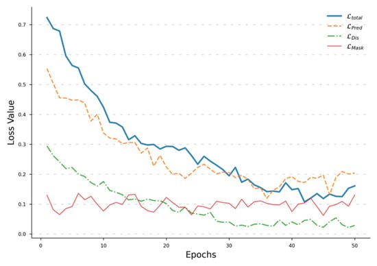
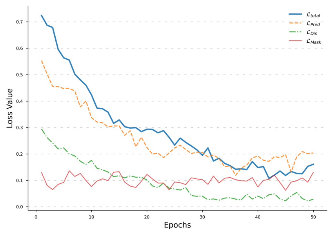
A system with four different losses usually raises questions about stability. We tracked the raw loss logs while training on the ETTm1 dataset to see if the different tasks would fight each other. Figure 2 shows the results. It can be observed that the training does not follow a simple, smooth path. Instead, it shows a complex evolutionary pattern that matches the task.

Figure 2. Convergence curves of different loss functions in this paper.

The red line for ${\mathcal{L}}_{Mask}$ is especially interesting because it stays in a controlled oscillation for all 50 epochs. This oscillation confirms the bi-level game from Algorithm 1. The mask generator is constantly testing the limits of the main network, which forces the backbone to find the most robust features.

The main prediction loss ${\mathcal{L}}_{\mathrm{Pr}ed}$ and the distillation loss ${\mathcal{L}}_{Dis}$ work well together. Even when the prediction fluctuates after epoch 35, the distillation path uses the Teacher model as an anchor to pull the system back to stability. By epoch 40, the total loss settles into a very tight envelope. Reaching this dynamic equilibrium proves that the multi-task setup is stable enough for regular retraining in the field.

3.5. Parameter Sensitivity

To find the best operating range for our framework, we looked at two main variables: the masking budget ρ and the prediction horizon T.

3.5.1. The Masking Budget

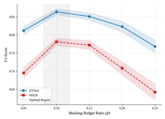
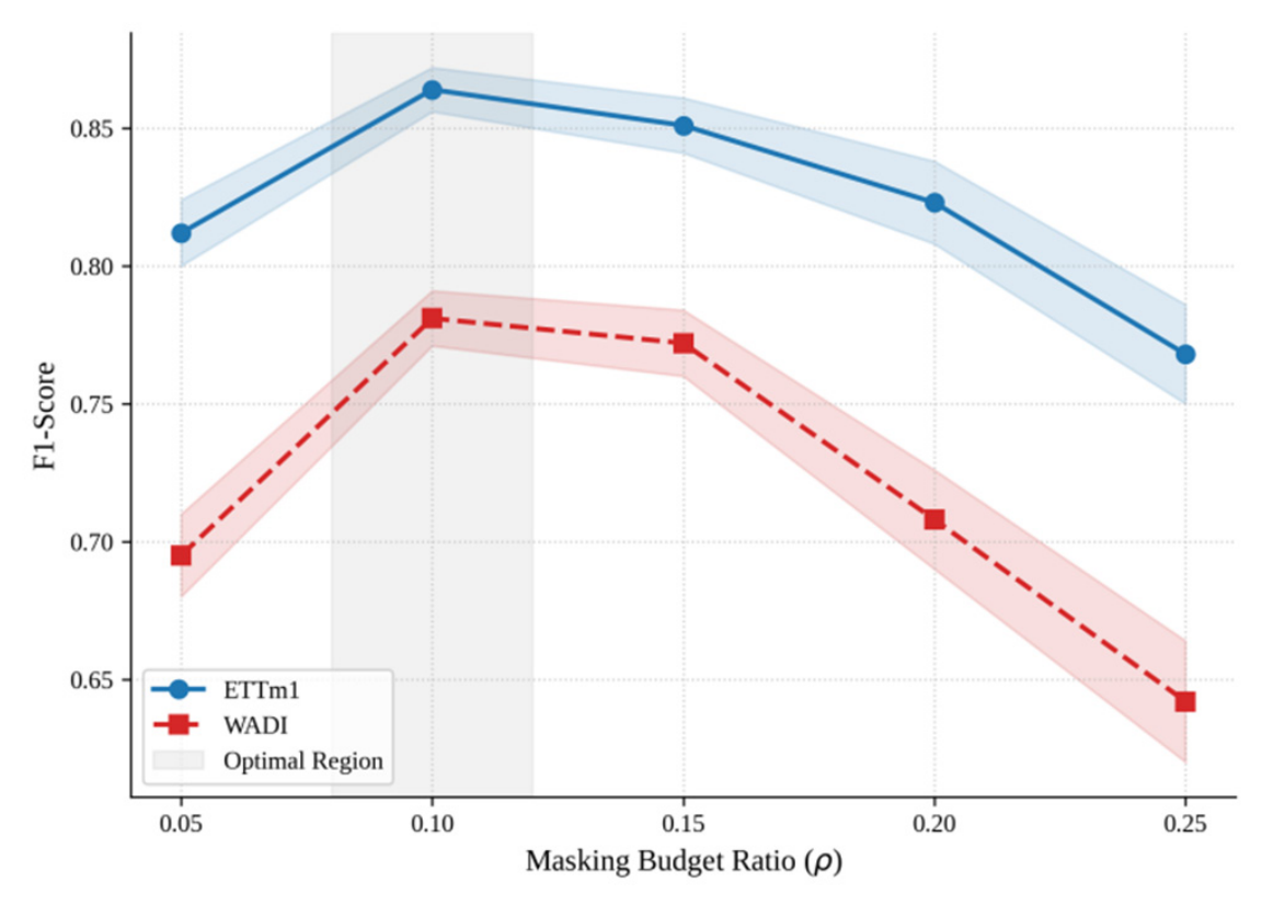
The masking budget ρ sets the limit for the information bottleneck in our bi-level optimization. It dictates how much temporal information the mask generator can hide to challenge the main network. We ran a gradient scan of ρ from 0.05 to 0.25 on ETTm1 and WADI, and the resulting performance curves are shown in Figure 3.

Figure 3. Sensitivity Analysis of the Masking Budget.

As shown in Figure 3, at a very low budget like 0.05, the results are not ideal. The physical reason is that the generator is too restricted to hide meaningful patterns. This allows the main network to rely on simple temporal neighbors for prediction rather than learning the deep spatio-temporal structure. We often see this as a kind of temporal dependency where the model avoids the hard task of feature decoupling. As ρ moves toward 0.1, the F1 score reaches its peak, which suggests that hiding about 10 percent of the information hits the information redundancy limit of these non-stationary power sequences.

The performance peak for WADI is notably sharper than ETTm1. This likely stems from the fact that 127 sensor nodes create massive feature redundancy, making the benefits of masking more pronounced. However, if we push ρ beyond 0.2, the system hits a fidelity crash. Over-masking destroys the causal logic needed to reconstruct the signal. The Predictor ends up guessing blindly because too many pieces of the puzzle are missing. We found that anchoring ρ at 0.1 keeps the features pure without losing the underlying waveform.

3.5.2. The Prediction Horizon

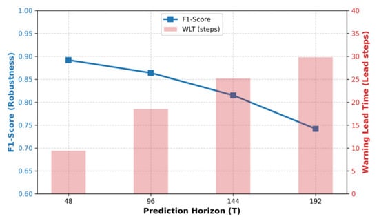
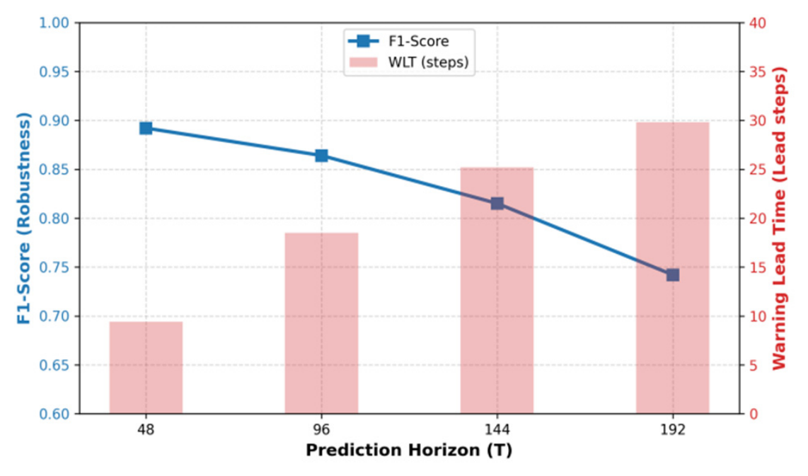
If the masking budget is about how clearly the model sees, the prediction horizon T is about how far it looks into the future. In substation maintenance, longer lead times are always better for dispatching crews, but extending the window increases the entropy of the prediction. We tested T from 48 to 192 steps to map out this trade-off, with the raw data and trends summarized in Table 8 and Figure 4.

Table 8. Performance trade-off across different prediction horizons in ETTm1 dataset.

T (Steps)	F1-Score	Lead Time WLT (Steps)	WLT in Physical Time (min)
48	0.892	9.4	141
96	0.864	18.5	277
144	0.815	25.2	378
192	0.742	29.8	447

Figure 4. Convergence curve.

Looking at the WLT values in Figure 4, the warning lead time grows almost linearly as we extend the prediction horizon T. At T = 192, the framework achieves nearly 7.4 h (29.8 steps) of pre-emptive reaction window. This near-linear scaling demonstrates that equipment health degradation leaves detectable, long-range trajectory shifts in the latent space well before physical breakdown occurs. However, the F1-score curve in Figure 4 reveals an accelerating accuracy decay beyond T = 144. From a physical modeling perspective, long-term autoregressive rollouts suffer from cumulative prediction entropy: as T expands, future load variability and phase shifts induce mode-mixing in predicted waveforms. These high-horizon prediction errors create artificial noise spikes in the Evaluator’s residual calculations, leading to occasional false alarms that drop the F1-score to 0.742 at T = 192.

It is worth noting that STF-MKD maintains higher stability across long horizons than baseline predictors because our Teacher-Guided distillation (TGAR) enforces strict manifold constraints. We identify T = 96 as the optimal engineering operating point: it provides an expansive 277 min (18.5-step) forewarning window for emergency load shedding while preserving a high F1-score of 0.864.

3.5.3. Robustness to Sensor Noise and Missing Data

In real-world power distribution substations, sensor streams are frequently corrupted by electromagnetic interference (EFT/surge noise) and packet dropouts during wireless transmission. To evaluate the fault tolerance of STF-MKD under corrupted observation conditions, we conducted stress tests on ETTm1 (T = 96) under two harsh synthetic scenarios: (1) Additive White Gaussian Noise with Signal-to-Noise Ratios (SNR) ranging from 30 dB down to 10 dB, and (2) Random Point Data Loss (Missing Data Rates from 10% to 30%). We benchmarked STF-MKD against three top-performing architectures: Fourier-KAN-Mamba, MambaAD, and iTransformer. The experimental results are summarized in Table 9.

Table 9. Robustness evaluation under additive noise and missing data on ETTm1 (T = 96).

Scenario	Condition	STF-MKD (Ours)	Fourier-KAN-Mamba	MambaAD	iTransformer
Baseline	Clean	0.864/18.5	0.831/14.2	0.815/9.6	0.804/7.2
Gaussian Noise	SNR = 30 dB	0.858/18.1	0.818/13.5	0.798/8.9	0.781/6.5
	SNR = 20 dB	0.842/17.2	0.792/11.8	0.765/7.8	0.732/4.8
	SNR = 10 dB	0.815/15.4	0.741/8.9	0.710/5.2	0.658/2.1
Missing Data	Rate = 10%	0.852/17.8	0.810/13.0	0.791/8.5	0.772/6.1
	Rate = 20%	0.835/16.5	0.778/10.9	0.752/6.9	0.715/4.2
	Rate = 30%	0.806/14.8	0.732/8.2	0.698/4.8	0.641/1.8

As shown in Table 9, STF-MKD exhibits superior physical immunity to both high-level sensor noise and random communication packet loss. Even under extreme electromagnetic noise (SNR = 10 dB), STF-MKD maintains an F1-score of 0.815 and a lead time of 15.4 steps, whereas iTransformer’s F1-score crashes to 0.658 with a lead time of only 2.1 steps. Similarly, under a 30% missing data rate, STF-MKD preserves over 93% of its baseline performance. This exceptional robustness is credited to the STF-Extractor’s dual-view dynamic masking and frequency filtering, which actively filters out unstructured noise spikes, as well as the WKAN Mexican Hat wavelets, which maintain sharp selectivity toward true structural fault singularities.

3.5.4. Impact of Pre-Training Dataset Contamination

To address the practical challenge where real-world historical logs may contain unlabelled, undetected micro-anomalies, we conducted a sensitivity experiment on ETTm1 (T = 96). We artificially injected unlabelled micro-anomalies (low-amplitude harmonic distortion and minor voltage drift) into the pre-training dataset ${\mathcal{X}}_{pure}$ at contamination ratios ranging from 0% (purified baseline) up to 10%. The resulting performance metrics are summarized in Table 10.

Table 10. Performance evaluation under pre-training dataset contamination on ETTm1 (T = 96).

Contamination Ratio	F1-Score	Lead Time WLT (Steps)	WLT in Physical Time (min)
0% (Purified Baseline)	0.864	18.5	277
1% Micro-anomalies	0.861	18.3	274
3% Micro-anomalies	0.852	17.8	267
5% Micro-anomalies	0.838	16.9	253
10% Micro-anomalies	0.795	14.2	213

As demonstrated in Table 10, STF-MKD exhibits substantial tolerance to training set contamination. When the contamination ratio remains below 5%, the F1-score experiences only a minor degradation (≤3.0%) and the physical warning lead time stays comfortably above 250 min. This resilience confirms that the combination of adaptive quantile clipping (3σ) and the smoothing property of WKAN B-splines effectively filters out micro-anomalies before they can alter the learned healthy manifold. Only when contamination reaches an extreme 10% does the Teacher’s reference manifold degrade noticeably, confirming that standard engineering purification (3σ thresholding) is sufficient for real-world IoT deployments.

3.5.5. Sensitivity of Loss Coefficients and Deployment Tuning Guide

To evaluate how the four loss balancing coefficients (λ_Pred, λ_Rec, λ_Dis, λ_M) interact and impact early warning accuracy, we performed a parameter sensitivity scan on ETTm1 (T = 96). By varying each coefficient around its default operating point (λ_Pred = 1.0, λ_Rec = 0.8, λ_Dis = 1.2, λ_M = 0.1) while holding others constant, we recorded the resulting F1-scores and Warning Lead Times (WLT). The quantitative scan results are summarized in Table 11.

Table 11. Loss coefficient interaction sensitivity scan on ETTm1 (T = 96).

Parameter Tested	Value Range	F1-Score Range	WLT Range (Steps)	Optimal Setting	Physical Impact/Trade-Off
λPred	0.5–1.5	0.812–0.864	14.1–18.5	1.0	Controls forecasting accuracy; under-scaling (<0.8) leads to prediction passivation.
λRec	0.4–1.2	0.835–0.864	16.2–18.5	0.8	Regulates Evaluator signal recovery; over-scaling (>1.0) forces fitting of noisy forecasts.
λDis	0.6–1.8	0.820–0.864	15.0–18.5	1.2	Anchors Evaluator to healthy Teacher manifold; essential for suppressing false alarms.
λM	0.05–0.25	0.795–0.864	11.6–18.5	0.1	Enforces dynamic masking budget ratio ρ; over-scaling (>0.2) causes fidelity collapse.

Based on these empirical findings, we provide a practical tuning guide for field engineers deploying STF-MKD across diverse grid environments:

High-Noise/Unstable Communication Substations: When sensors suffer from severe electromagnetic interference or packet dropouts, engineers should increase feature distillation weight λ_Dis to 1.4–1.5. This strengthens the Teacher’s anchor, shielding the Evaluator from prediction noise.

Critical Asset Monitoring (Zero-Fault Tolerance): For high-value assets like main power transformers where missing a precursor is catastrophic, increase prediction guidance weight λ_Pred to 1.2–1.4. This forces the Predictor to focus more aggressively on faint anomaly precursors.

High-Dimensional Multi-Sensor Nodes (e.g., 100+ Channels): In complex substations with dense spatial dependencies, strictly keep the masking sparsity penalty λ_M ≈ 0.1. Over-constraining λ_M disrupts spatial graph decoupling and causes information bottlenecks.

3.6. Case Studies

Quantitative metrics provide a solid base for STF-MKD, but these numbers do not always show what the model actually sees during a warning event. We pulled a representative overload segment from the ETTm1 dataset to walk through the journey from normal operation to a structural breakdown. This section uses multi-scale visualizations to show how our framework moves from simple observation to true foresight.

3.6.1. Alignment of Anomaly Scores and Raw Waveforms

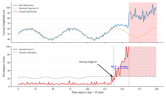
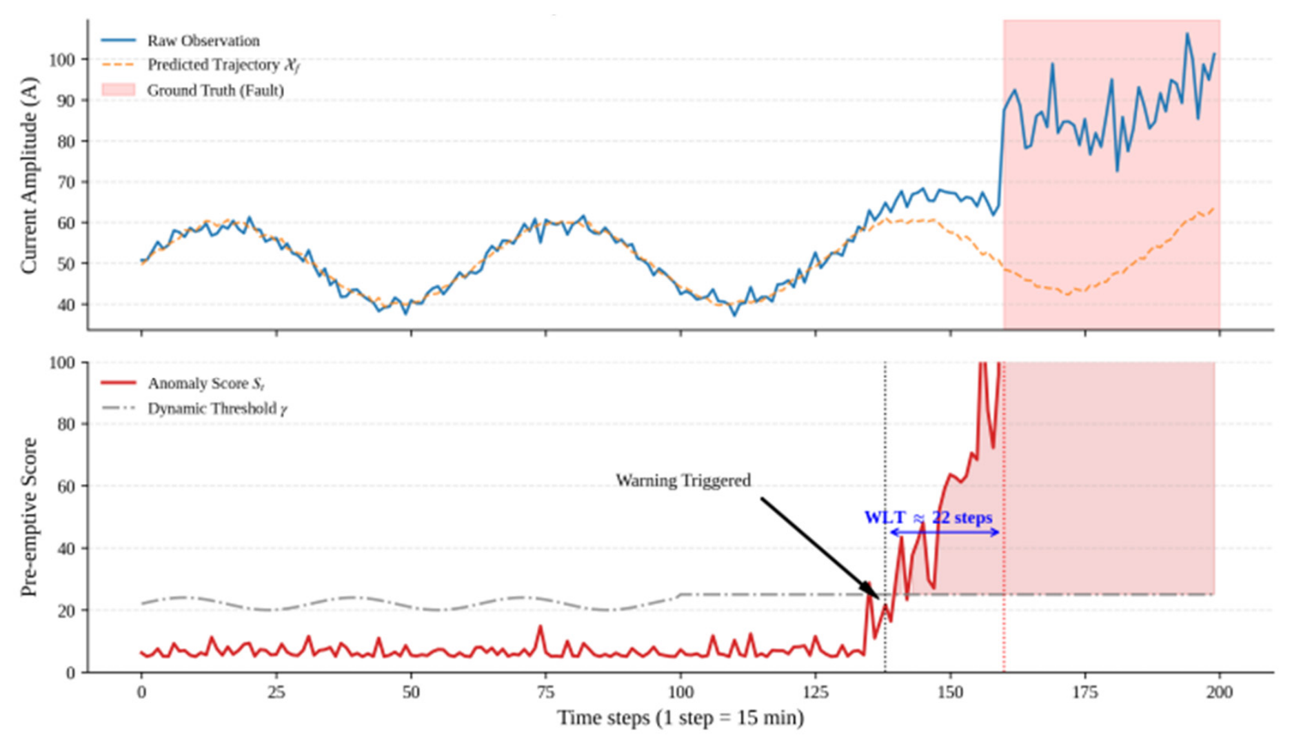
Figure 5 tracks the dynamic performance of the model during a fault incubation period. As shown in the top plot, the physical fault manifests at time step 160. Approximately 450 min prior (around step 130), the raw current observation (blue line) exhibits an unsteady upward drift. However, because this drift remains within the amplitude envelope of normal peak loads, conventional static threshold detectors fail to trigger. In contrast, our predicted trajectory (orange dashed line) diverges noticeably. Because the Predictor and Evaluator are strictly anchored to the healthy physical manifold via Teacher-guided distillation, the model recognizes that this drift violates the learned nonlinear power conservation laws and refuses to follow the abnormal signal trajectory. This divergence forms a visible “residual cavity” between the observed drift and the expected healthy trajectory.

Figure 5. Case study.

This physical mismatch triggers early-warning pulses in the pre-emptive anomaly score S_t shown in the bottom plot of Figure 5. The score S_t (red line) climbs rapidly 330 min prior to physical failure. At step 138, S_t punches through the dynamic threshold γ generated by the SPOT algorithm, issuing a formal early warning. Crucially, the SPOT γ (dash-dot gray line) dynamically adapts to background load variance, rising slightly during normal load surges to suppress false alarms, yet remaining sensitive enough to be breached the moment structural risk accumulates.

Achieving a Warning Lead Time (WLT) of 22 steps (5.5 h) grants grid operators ample time to perform controlled load dispatch or crew deployment before hardware failure occurs. In contrast, most baseline models only catch the defect around step 150 when the current surge becomes blatantly obvious, leaving insufficient reaction window for emergency response. Buying this much advance notice represents the practical difference between a controlled load shift and catastrophic hardware destruction.

3.6.2. Tracking the Feature Purification of the Mask Generator

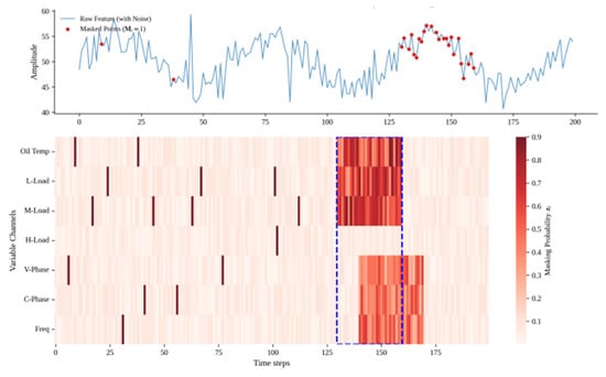
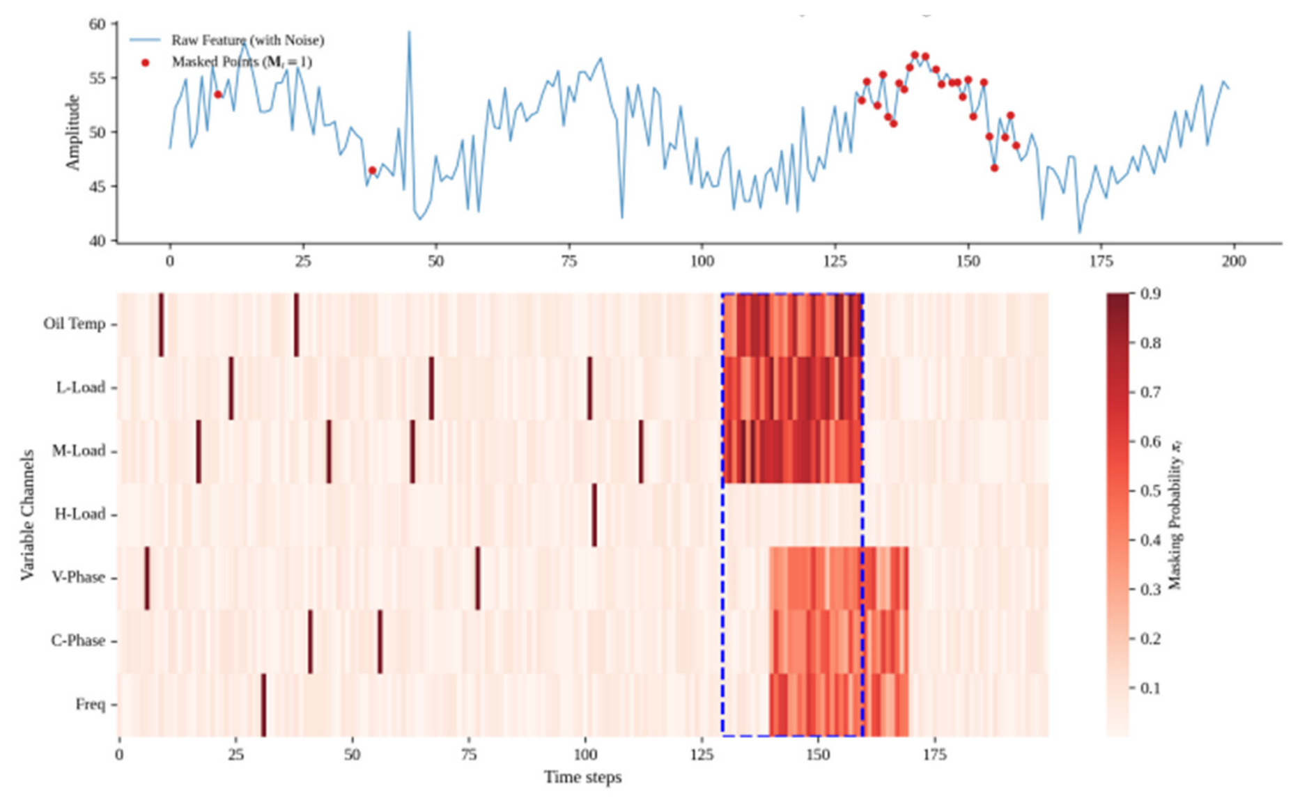
We visualized the mask distribution in Figure 6 to confirm if the STF-Extractor is truly filtering the noise. This step helps us see what the model chooses to ignore and what it keeps.

Figure 6. Information bottleneck via dynamic masking.

Figure 6 illustrates the adaptive operation of the STF-Extractor’s mask generator G_mask under an information bottleneck constraint. The top subplot shows that during steady-state operation (steps 0–120), G_mask assigns hard mask points (M_t = 1, red dots) sparsely to isolated, high-frequency noise spikes, functioning as an adaptive spatial-temporal denoiser. However, as the fault incubation period commences at step 130, the mask generator dramatically increases mask density, purposefully targeting the nonlinear inflection points induced by the developing overload.

The probability heatmap π_t in the bottom plot of Figure 6 provides deep physical interpretability. Within the warning zone (steps 130–160, As shown in the dashed square in the Figure 6), the Oil Temp and L-Load (Low-voltage Load) channels exhibit the darkest red hues, receiving the highest masking probabilities (π_t > 0.85). This pattern directly reflects transformer degradation thermodynamics: electrical current overload and oil thermal inertia are the earliest physical indicators of impending failure, exhibiting nonlinear structural drift long before voltage collapse. In contrast, the V-Phase (Voltage Phase) channel exhibits lagging masking intensity. By deliberately hiding the most informative, structurally unstable channels during incubation, the bi-level masking game forces the backbone to reconstruct missing context via multi-node spatial graph topology, making the representations exceptionally robust against single-sensor noise while highlighting the physical root cause of the fault.

3.6.3. Proving the Multi-Scale Decoupling of Mamba-WKAN

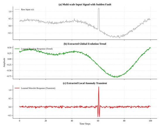
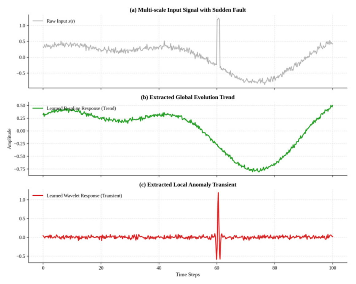
To understand why STF-MKD is so effective at catching transients, we looked at the dynamic response of the WKAN operators, and Figure 7 shows how the model breaks down a complex input signal into its core components.

Figure 7. WKAN decomposition response.

Figure 7 demonstrates the multi-scale operator-level signal decomposition achieved by the Mamba-WKAN backbone. The raw input signal in Figure 7a captures complex grid operating dynamics: a smooth daily load cycle combined with high-frequency noise and a sharp, localized overload transient at t = 60.

Figure 7b highlights the B-spline branch response (green curve), which displays complete structural immunity to the transient spike at t = 60. Because B-splines rely on Cox-de Boor piecewise polynomial recursion, they act as low-pass physical filters that capture global continuous trends while ignoring isolated singularities. This immunity guarantees that sudden, benign load switching events do not distort the learned baseline trend, suppressing false positive warnings.

Conversely, Figure 7c shows the Mexican Hat wavelet branch response (red curve). Because the Mexican Hat wavelet mathematically represents the second derivative of a Gaussian, it remains completely zeroed during smooth steady-state operation but strongly resonates at t = 60 with an intense bipolar impulse. This mathematical selectivity grants the backbone micro-second reflexes toward signal singularities that signal arcing or insulation breakdown, which standard MLPs or polynomial smoothers smooth away.

We define this specialized division of labor as “spline-locking for smooth trends and wavelet-catching for sharp transients.” This parallel operator-level decoupling ensures that the final anomaly score S_t stays completely flat during normal operation while reacting instantly to real structural fault precursors.

4. Conclusions

We addressed the persistent issues of lag and nonlinear feature capture in power IoT anomaly detection by fusing state-space models with nonlinear operators. Through the development of the STF-MKD framework, we have built a system capable of genuine foresight. Our findings from the theoretical and empirical analysis can be summarized in three main points.

First, we confirmed that using physical priors to separate architecture is the most effective way to handle noise in the grid. The STF-Extractor cleans up the feature stream by blending graph topology, temporal masking, and frequency purification. By stripping away normal load swings at the earliest stage, we provide the rest of the model with a pure data stream, which naturally lowers the chance of false alarms. Second, the synergy between Mamba and WKAN sets a new standard for both speed and accuracy in long-sequence tasks. The data challenges the common belief that high accuracy requires massive, slow models. Because wavelets are so sensitive to signal spikes, STF-MKD handles high-dimensional monitoring much faster than Transformer-based designs. This approach makes the model more transparent for engineers, as they can see exactly how the splines track trends and wavelets catch bursts.

Third, our teacher–student distillation creates a new way to handle early warning when labeled data is missing. By creating an information gap between an omniscient teacher and a real-time student, the TGAR mechanism pulls future risks back into the current feature space. The significant jump in lead times proves that the system is truly learning the evolution of faults rather than just making lucky guesses. Of course, the grid is always changing, and our next step involves looking at incremental learning to handle the different types of hardware found in the field.

References

- Rouholamini, M.; Wang, C.; Magableh, S.; Wang, X. Resiliency of electric power distribution networks: A review. J. Infrastruct. Preserv. Resil. 2025, 6, 39. [Google Scholar] [CrossRef] [Scilit]
- Ahmed, F.; Ahmad, S.; Rahman, M.T.; Hazari, R.; Faiz, R.; Ahmed, T.; Karimi, M. A holistic review of electric vehicle charging impacts on power distribution networks: Technical challenges, smart mitigation strategies and future directions. Appl. Energy 2026, 402, 126961. [Google Scholar] [CrossRef] [Scilit]
- Hamdeen, I.; Badran, E.A.; Kotb, M.F.; Elgamal, M. Self-healing multi-agent techniques in electric power distribution systems: A review. Renew. Sustain. Energy Rev. 2025, 224, 116132. [Google Scholar] [CrossRef] [Scilit]
- Noman, A.A.; Baidya, P.; Hossain, M.A.; Dev, P.; Saha, K.; Hossain, M. Design and Implementation IoT-Driven Distribution Transformer Health Monitoring System for the Smart Power Grid. Eng. Proc. 2025, 87, 27. [Google Scholar] [CrossRef] [Scilit]
- Luo, T.; Nagarajan, S.G. Distributed anomaly detection using autoencoder neural networks in WSN for IoT. In Proceedings of the 2018 IEEE International Conference on Communications (ICC), Kansas City, MO, USA, 20–24 May 2018; IEEE: New York, NY, USA, 2018; pp. 1–6. [Google Scholar]
- Thanigaivelan, N.K.; Nigussie, E.; Kanth, R.K.; Virtanen, S.; Isoaho, J. Distributed internal anomaly detection system for Internet-of-Things. In Proceedings of the 2016 13th IEEE Annual Consumer Communications & Networking Conference (CCNC), Las Vegas, NV, USA, 9–12 January 2016; IEEE: New York, NY, USA, 2016; pp. 319–320. [Google Scholar]
- Pahl, M.O.; Aubet, F.X. All eyes on you: Distributed Multi-Dimensional IoT microservice anomaly detection. In Proceedings of the 2018 14th International Conference on Network and Service Management (CNSM), Rome, Italy, 5–9 November 2018; IEEE: New York, NY, USA, 2018; pp. 72–80. [Google Scholar]
- Yu, F.; Guo, Q.; Wu, J.; Qiao, Z.; Sun, H. Early warning and proactive control strategies for power blackouts caused by gas network malfunctions. Nat. Commun. 2024, 15, 4714. [Google Scholar] [CrossRef] [Scilit] [PubMed]
- Yu, F.; Guo, Q.; Wang, B.; Zhao, H.; Sun, Y.; Li, D. Refined early warning and proactive control framework of gas-electric cascading failures based on dynamic equivalence of gas networks. CSEE J. Power Energy Syst. 2026, 1–14. [Google Scholar] [CrossRef]
- Choi, H.T.; Park, H.Y.; Kim, T.; Kim, J.H. A Novel Anomaly Forecasting in Time-Series Data: Feedback Connection between Forecasting and Detecting Algorithms with Applications to Power Systems. Adv. Intell. Syst. 2025, 7, 2401141. [Google Scholar] [CrossRef] [Scilit]
- Dzafic, D.; Džafić, I.; Akagic, A. Anomaly detection in smart grid time-series data using Graph Deviation Networks. Eng. Appl. Artif. Intell. 2026, 165, 113512. [Google Scholar] [CrossRef] [Scilit]
- Ta, X.; Liu, Z.; Hu, X.; Yu, L.; Sun, L.; Du, B. Adaptive spatio-temporal graph neural network for traffic forecasting. Knowl.-Based Syst. 2022, 242, 108199. [Google Scholar] [CrossRef] [Scilit]
- Zhang, Q.; Liu, J.; Xie, K.; Liu, Q. A dynamic spatio-temporal graph neural network with global and local perception for remaining useful life prediction. Expert Syst. Appl. 2025, 282, 127707. [Google Scholar] [CrossRef] [Scilit]
- Liu, Y.; Hu, T.; Zhang, H.; Wu, H.; Wang, S.; Ma, L.; Long, M. itransformer: Inverted transformers are effective for time series forecasting. arXiv 2023, arXiv:2310.06625. [Google Scholar]
- Nie, Y.; Nguyen, N.H.; Sinthong, P.; Kalagnanam, J. A time series is worth 64 words: Long-term forecasting with transformers. arXiv 2022, arXiv:2211.14730. [Google Scholar]
- Karkhaneh, M.; Ozgoli, S. Anomalous load profile detection in power systems using wavelet transform and robust regression. Adv. Eng. Inform. 2022, 53, 101639. [Google Scholar] [CrossRef] [Scilit]
- Carratù, M.; Gallo, V.; Iacono, S.D.; Sommella, P.; Bartolini, A.; Grasso, F.; Ciani, L.; Patrizi, G. A novel methodology for unsupervised anomaly detection in industrial electrical systems. IEEE Trans. Instrum. Meas. 2023, 72, 1–12. [Google Scholar] [CrossRef] [Scilit]
- Wang, Z.; Kong, F.; Feng, S.; Wang, M.; Yang, X.; Zhao, H.; Wang, D.; Zhang, Y. Is mamba effective for time series forecasting? Neurocomputing 2025, 619, 129178. [Google Scholar] [CrossRef] [Scilit]
- Patro, B.N.; Agneeswaran, V.S. Simba: Simplified mamba-based architecture for vision and multivariate time series. arXiv 2024, arXiv:2403.15360. [Google Scholar]
- Wang, X.; Wang, L.; Wang, R.; Zhang, Z.; Zhao, M. Fourier-KAN-Mamba: A Novel State-Space Equation Approach for Time-Series Anomaly Detection. arXiv 2025, arXiv:2511.15083. [Google Scholar]
- Cheng, W.; Li, Y.; Ma, T. S-KDGAN: Series-knowledge distillation with GANs for anomaly detection of sensor time-series data in smart IoT. IEEE Sens. J. 2024, 24, 24344–24354. [Google Scholar] [CrossRef] [Scilit]
- Xu, Q.; Chen, Z.; Ragab, M.; Wang, C.; Wu, M.; Li, X. Contrastive adversarial knowledge distillation for deep model compression in time-series regression tasks. Neurocomputing 2022, 485, 242–251. [Google Scholar] [CrossRef] [Scilit]
- Liu, C.; He, S.; Zhou, Q.; Li, S.; Meng, W. Large language model guided knowledge distillation for time series anomaly detection. arXiv 2024, arXiv:2401.15123. [Google Scholar]
- Babbar, V.; McTavish, H.; Rudin, C.; Seltzer, M. Near optimal decision trees in a SPLIT second. arXiv 2025, arXiv:2502.15988. [Google Scholar]
- Zhou, H.; Zhang, S.; Peng, J.; Zhang, S.; Li, J.; Xiong, H.; Zhang, W. Informer: Beyond efficient transformer for long sequence time-series forecasting. Proc. AAAI Conf. Artif. Intell. 2021, 35, 11106–11115. [Google Scholar] [CrossRef] [Scilit]
- Goh, J.; Adepu, S.; Junejo, K.N.; Mathur, A. A dataset to support research in the design of secure water treatment systems. In International Conference on Critical Information Infrastructures Security; Springer International Publishing: Cham, Switzerland, 2016; pp. 88–99. [Google Scholar]
- Ahmed, C.M.; Palleti, V.R.; Mathur, A.P. WADI: A water distribution testbed for research in the design of secure cyber physical systems. In Proceedings of the 3rd International Workshop on Cyber-Physical Systems for Smart Water Networks, Pittsburgh, PA, USA, 21 April 2017; Association for Computing Machinery: New York, NY, USA, 2017; pp. 25–28. [Google Scholar]
- Qin, S.; Zhu, J.; Guo, A.; Yang, Y.; Wang, L.; Tao, G. MambaAD: Multivariate time series anomaly detection in IoT via multi-view Mamba. Neurocomputing 2025, 655, 131385. [Google Scholar] [CrossRef] [Scilit]
- Xu, J.; Wu, H.; Wang, J.; Long, M. Anomaly transformer: Time series anomaly detection with association discrepancy. arXiv 2021, arXiv:2110.02642. [Google Scholar]
- Luo, D.; Wang, X. ModernTCN: A Modern Pure Convolution Structure for General Time Series Analysis. In Proceedings of the International Conference on Learning Representations 2024 (ICLR 2024), Vienna, Austria, 7–11 May 2024. [Google Scholar]
- Wu, H.; Hu, T.; Liu, Y.; Zhou, H.; Wang, J.; Long, M. Timesnet: Temporal 2d-variation modeling for general time series analysis. arXiv 2022, arXiv:2210.02186. [Google Scholar]
- Fourure, D.; Javaid, M.U.; Posocco, N.; Tihon, S. Anomaly detection: How to artificially increase your f1-score with a biased evaluation protocol. In Joint European Conference on Machine Learning and Knowledge Discovery in Databases; Springer International Publishing: Cham, Switzerland, 2021; pp. 3–18. [Google Scholar]
- Pang, G.; Shen, C.; Van Den Hengel, A. Deep anomaly detection with deviation networks. In Proceedings of the 25th ACM SIGKDD International Conference on Knowledge Discovery & Data Mining, Anchorage, AK, USA, 4–8 August 2019; Association for Computing Machinery: New York, NY, USA, 2019; pp. 353–362. [Google Scholar]
- Kim, S.; Choi, K.; Choi, H.S.; Lee, B.; Yoon, S. Towards a rigorous evaluation of time-series anomaly detection. Proc. AAAI Conf. Artif. Intell. 2022, 36, 7194–7201. [Google Scholar] [CrossRef] [Scilit]
Disclaimer/Publisher’s Note: The statements, opinions and data contained in all publications are solely those of the individual author(s) and contributor(s) and not of MDPI and/or the editor(s). MDPI and/or the editor(s) disclaim responsibility for any injury to people or property resulting from any ideas, methods, instructions or products referred to in the content. |
© 2026 by the authors. Licensee MDPI, Basel, Switzerland. This article is an open access article distributed under the terms and conditions of the Creative Commons Attribution (CC BY) license.