Hybrid Quantum Recurrent Neural Network for Remaining Useful Life Prediction of Turbofan Engines

Abstract

Accurate remaining useful life (RUL) estimation underpins safe operation and cost-effective maintenance of aerospace propulsion systems. We propose a Hybrid Quantum Recurrent Neural Network (HQRNN) for jet-engine RUL forecasting on the NASA C-MAPSS FD001 benchmark. The HQRNN stacks Quantum Long Short-Term Memory (QLSTM) layers, replacing each LSTM gate’s linear transformation with a Quantum Depth-Infused (QDI) circuit; this is followed by classical dense layers. Quantum and hybrid quantum–classical methods for turbofan RUL prediction are still at an early stage. Our study is therefore among the first to evaluate a gate-based QLSTM hybrid at matched parameter counts, comparing it against classical and joint state-of-the-art models on this benchmark and complementing that comparison with a circuit-level analysis of the quantum layer. Encoding the gate signals in a quantum feature space is intended to help the network represent high-frequency degradation patterns with fewer trainable parameters than a matched classical counterpart. The HQRNN improves mean RMSE and mean MAE by about $5\%$ over matched-parameter stacked-LSTM RNNs across 10 random seeds, and attains a test RMSE of $15.46$, outperforming Random Forest, CNN, and MLP baselines. ZX calculus, Fisher information, and Fourier analyses indicate that the QDI circuit is compact, trainable, and expressive. Advanced joint deep-learning models still outperform the stand-alone HQRNN, indicating that quantum-enhanced recurrent modules are best deployed as components within composite prognostics pipelines rather than stand-alone predictors.

1. Introduction

Accurate estimation of the remaining useful life (RUL) of safety-critical machinery is a cornerstone of modern reliability and risk-management strategies [1,2,3]. Nowhere is this more evident than in commercial aviation, where the timely prediction of gas-turbine jet engine failures both prevents catastrophic breakdowns [4] and streamlines maintenance and resource allocation [5]. Robust forecasting models enable operators to defer costly repairs until necessary while avoiding the risks of overdue overhauls, ultimately reducing downtime and improving fleet utilisation [6,7].

Time-series methods for RUL estimation can be broadly categorised into statistical and machine-learning approaches. Traditional statistical methods such as autoregressive, moving-average and ARIMA models excel under stationarity and linearity assumptions [8,9] but struggle to capture the non-linear, interdependent patterns characteristic of real-world aerospace data [10]. Within machine learning, recurrent neural networks (RNNs) and, in particular, Long Short-Term Memory (LSTM) networks [11,12,13,14] have become standard tools for capturing temporal dependencies in degradation signals [15].

Despite these successes, classical machine-learning strategies can be weakened by limited or noisy run-to-failure data, high-dimensional feature spaces, and intricate fault dynamics [16,17]. These conditions are routine in industrial prognostics: run-to-failure datasets are expensive to acquire, often containing only tens or hundreds of full trajectories, and sensor readings are noisy and correlated. Methods that can generalise well from limited data are therefore highly desirable.

Quantum computing has recently progressed from theoretical constructs to initial practical demonstrations, leveraging entanglement and superposition to enable computational processes beyond conventional hardware [18,19,20,21]. Quantum machine learning (QML) emerged at the intersection of these two fields, with theoretical and empirical evidence that QML models can address problems characterised by constrained datasets or high-dimensional feature spaces [22,23,24,25,26]. QML leverages high-dimensional Hilbert spaces to encode input features, allowing more complex patterns to be represented with fewer parameters than classical counterparts [27,28]. This is particularly beneficial when applied to non-stationary or noisy signals frequently encountered in industrial maintenance and prognostic applications [29,30].

Hybrid quantum–classical neural networks (HQNNs) combine classical and quantum machine learning within a single framework [31,32,33,34,35,36]. The quantum component plays a specific role in feature encoding or transformation while leaving backpropagation and parameter optimisation to classical routines [37]. Preliminary studies indicate that HQNNs can match or exceed the performance of their classical counterparts [38,39], often exhibiting greater resilience to overfitting [40,41]. The inherent parameter efficiency of HQNNs further enhances their suitability for scenarios involving complex, high-dimensional inputs or limited data availability, conditions that are typical in predictive maintenance.

Data-driven prognostics of aero-engines has matured over more than a decade, with the NASA C-MAPSS dataset [42,43] serving as the de facto benchmark. Early studies applied conventional machine-learning models (Random Forest, LASSO regression, Support Vector Machines, k-nearest-neighbour regression, and Gradient Boosting [4]), which provide interpretable baselines but cannot natively model long-range temporal structure in the sensor signals. Deep-learning approaches, including Multilayer Perceptrons, Convolutional Neural Networks [44], and LSTM-based recurrent models [45], explicitly capture temporal dependencies yet still saturate at moderate RMSE on the relatively small FD001 subset. The current state of the art combines complementary architectures with sophisticated feature preprocessing: Temporal Convolutional Networks coupled with Transformers [46], attention-aware CNN–LSTM models [47], broad-learning systems fused with TCNs [48], FCLCNN–LSTM hybrids [49], and Auto-RUL-augmented LSTMs [50], achieving the lowest reported RMSE on FD001 at the cost of substantially more parameters and preprocessing complexity.

While quantum–classical hybrids have been explored in finance [29], energy forecasting [30,51], materials science [52], and healthcare [53], their use in industrial prognostics is still at an early stage. A small but growing body of work has begun to apply quantum, hybrid, and quantum-inspired methods to the C-MAPSS benchmark, and QLSTM variants such as that of Chen et al. [54] provide the algorithmic foundation. To the best of our knowledge, however, gate-based hybrid recurrent models have not yet been systematically benchmarked at matched parameter counts against the classical and joint state of the art on standard C-MAPSS protocols. The present work contributes to this emerging area with such a comparison and a circuit-level analysis of the quantum layer.

This paper proposes and evaluates a Hybrid Quantum Recurrent Neural Network (HQRNN) tailored for jet-engine RUL forecasting on the NASA Commercial Modular Aero-Propulsion System Simulation (C-MAPSS) benchmark [42,43]. Our specific contributions are as follows:

1.

We introduce a Quantum Long Short-Term Memory (QLSTM) architecture in which the linear transformation within each LSTM gate is replaced by a Quantum Depth-Infused (QDI) circuit [30,53,54,55,56].

2.

We empirically demonstrate that, at matched parameter budgets, the HQRNN improves average RMSE and MAE by approximately $5\%$ over classical LSTM-based RNNs on the C-MAPSS FD001 subset, despite using fewer trainable parameters in some configurations.

3.

We benchmark the HQRNN against classical machine-learning baselines (Random Forest, LASSO, SVM, KNR, Gradient Boosting), simple neural-network baselines (MLP, CNN, LSTM), and several recent joint deep-learning architectures, situating the proposed method within the current state-of-the-art landscape for the C-MAPSS benchmark.

4.

We analyse the QDI quantum circuit through three complementary perspectives (ZX calculus, Fisher information, and Fourier expressivity) to verify that the chosen circuit is parameter-efficient, well-trainable, and capable of representing high-frequency components relevant to degradation modelling.

The remainder of the paper is organised as follows. Section 2 describes the C-MAPSS dataset and the prognostic problem formulation. Section 3 introduces the HQRNN architecture and the QDI circuit. Section 4 details the experimental setup and reports the empirical results. Section 5 analyses the quantum circuit. Section 6 discusses implications for prognostics pipelines, and Section 7 concludes the paper.

2. Dataset and Problem Formulation

The NASA C-MAPSS dataset [42] is a widely used multivariate time-series benchmark for analysing gas-turbine engine degradation. In this work we employ the FD001subset, which contains run-to-failure data for a fleet of 100 turbofan engines. Each engine progresses from a nominal state to the point of failure, providing sensor measurements over multiple cycles.

The C-MAPSS data are produced by a high-fidelity thermo-dynamical simulation of a commercial turbofan engine [42,43]. Each trajectory starts from a healthy engine with small, randomly assigned initial wear and manufacturing variation and degrades under a prescribed fault until a failure threshold is reached, with the recorded sensor outputs corrupted by measurement noise. The FD001 subset corresponds to a single operating condition and a single fault mode (high-pressure-compressor degradation), which makes it the most controlled, and hence the most widely reported, of the four C-MAPSS subsets.

The dataset comprises four main feature groups:

1.

An engine identifier (ranging from 1 to 100);

2.

A time index in cycles;

3.

Three operational settings;

4.

Twenty-one sensor measurements.

For simplicity, we exclude the operational settings and focus on the sensor measurements for predicting RUL. More sophisticated feature-selection schemes, including hybrid quantum–classical selectors [57], could further prune the input set, but are beyond the scope of this study.

The C-MAPSS benchmark is distributed already partitioned into a training set and a test set. This dataset-level split is the one provided by NASA and should not be confused with the train/validation split that we later carve out of the training set for model development (Section 4). In the provided training set, each engine’s sensor measurements are recorded until failure, whereas in the test set the measurements end at an arbitrary cycle prior to failure. The prognostic task is to predict the number of remaining operational cycles before failure for each test engine, and a vector of ground-truth RUL values for the test data is provided for evaluation.

We design our predictive model as follows. The model receives a fixed-size window of consecutive engine cycles as input and yields a single estimated RUL value as output. This means that for each entry in the training dataset there should be a corresponding target RUL value.

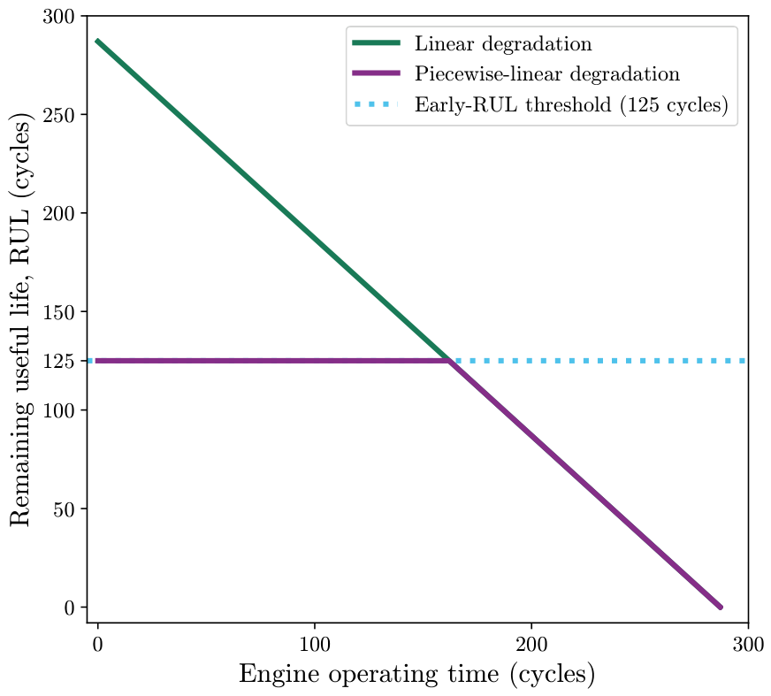
Creation of these RUL values depends on the degradation model. A linear degradation model decreases the RUL linearly to zero as the engine approaches failure. In this work we instead use a piecewise-linear degradation model. It assumes that the engine operates normally for an initial period, during which the RUL is held constant (the “early-RUL” regime), and then develops a fault, after which its useful life decreases linearly (see Figure 1). We set the early-RUL threshold to 125 cycles, based on the minimum run length of 128 cycles observed in the training data.

Upon inspecting the training data, we found that seven of the twenty-one sensor channels ($s_1,s_5,s_6,s_{10},s_{16},s_{18},s_{19}$) remain constant across all cycles and therefore carry no predictive information. Together with the three operational-setting channels, these are removed, leaving 14 informative sensor channels ($s_2,s_3,s_4,s_7,s_8,s_9,s_{11},s_{12},s_{13},s_{14},s_{15},s_{17},s_{20},s_{21}$). Each retained channel is standardised to zero mean and unit variance (z-score normalisation); the scaler statistics are estimated on the training data only and then applied unchanged to the test data, so no test information influences preprocessing.

Because our proposed architecture relies on LSTM-like layers, we segment each time series into windows of length 30 cycles. Each window is therefore a $30\times 14$ matrix of sensor values. The network takes this window as input and produces a single RUL estimate for the cycle immediately following the window, yielding a supervised learning setup for the engine-degradation problem.

3. Hybrid Quantum Recurrent Neural Network

The proposed HQRNN comprises a stack of Quantum Long Short-Term Memory (QLSTM) layers followed by classical fully connected layers for final regression. The QLSTM layer is derived from the conventional LSTM by substituting the linear transformations in each of the four gates (forget, input, update, output) with a Quantum Depth-Infused (QDI) layer.

Classical deep neural networks often bias their learning towards lower-frequency components, a phenomenon sometimes referred to as the “F-Principle” [58]. Angle-encoded quantum circuits such as the QDI layer can be interpreted as operating in a Fourier-transformed feature space [59], which may make it easier to represent higher-frequency components. We treat this as a motivating inductive bias rather than a proven advantage; the empirical comparisons in Section 4 and the circuit-level analysis in Section 5 are what we rely on.

3.1. Architecture Overview

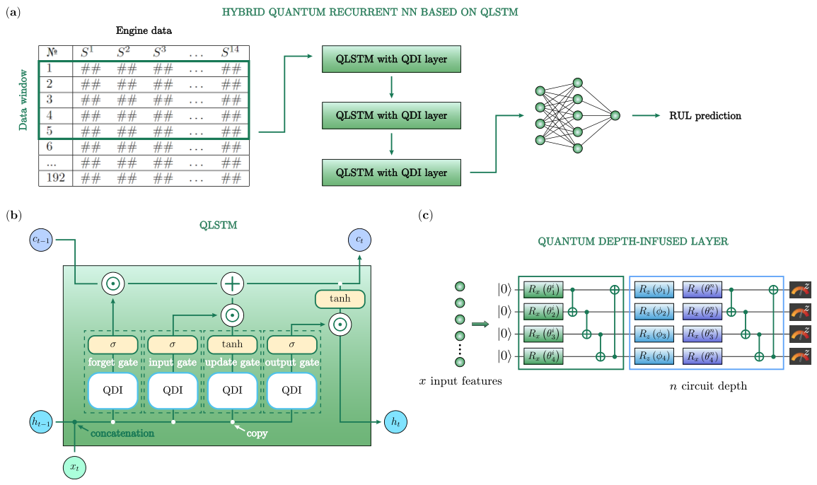
Figure 2 provides an overview of the HQRNN model and its constituent layers. Figure 2a shows the complete pipeline: an input window of sensor measurements of size $W\times 14$ (where $W=30$ is the window length and 14 is the number of sensor features) is passed through three stacked QLSTM layers with latent dimensions of 32, 16, and 8 respectively. The output of the QLSTM stack is then fed into classical dense layers that reduce the dimension from $8\times W$ to 16, then 32, and finally to a single scalar value representing the predicted RUL. Figure 2b depicts the internal structure of a single QLSTM layer, highlighting the replacement of each conventional linear gate transformation with an individual QDI layer.

Crucially, each gate of the QLSTM is not a bare quantum circuit but a classical–quantum–classical composition, and the QDI circuits never receive raw sensor readings. Let $x_t\in {\mathbb{R}}^{d_{\mathrm{in}}}$ denote the input at time step t of a QLSTM layer with hidden size $d_h$, and let $h_{t-1},c_{t-1}\in {\mathbb{R}}^{d_h}$ be the previous hidden and cell states. The cell first forms a classical linear input projection

$$v_t=W_x{x}_t+W_h{h}_{t-1},v_t\in {\mathbb{R}}^{4m},$$

(1)

where $m=n_{q}L=4$ is the QDI input width ($n_q=4$ qubits and $L=1$ encoding repetition), and $W_x\in {\mathbb{R}}^{4m\times d_{\mathrm{in}}}$, $W_h\in {\mathbb{R}}^{4m\times d_h}$ are trainable weight matrices that together form the input projector. The vector $v_t$ is split into four gate input projections $a_t^f,a_t^i,a_t^g,a_t^o\in {\mathbb{R}}^m$, one per gate. Each gate passes its input projection through a QDI circuit and a shared linear readout $\mathrm{clayer}\_\mathrm{out}:{\mathbb{R}}^{n_q}\to {\mathbb{R}}^{d_h}$,

$$z_t^{\gamma }=\mathrm{clayer}\_\mathrm{out}\left({\mathrm{QDI}}_{\gamma }(a_t^{\gamma })\right),\gamma \in \{f,i,g,o\},$$

(2)

where ${\mathrm{QDI}}_{\gamma }:{\mathbb{R}}^m\to {\mathbb{R}}^{n_q}$ is the four-qubit circuit of Section 3.2. The standard LSTM recurrence then follows,

$$\begin{array}{cc}\hfill f_t& =\sigma (z_t^f),i_t=\sigma (z_t^i),g_t=\tanh (z_t^g),o_t=\sigma (z_t^o),\hfill \end{array}$$

(3)

$$\begin{array}{cc}\hfill c_t& =f_t\odot c_{t-1}+i_t\odot g_t,h_t=o_t\odot \tanh (c_t),\hfill \end{array}$$

(4)

with $\sigma$ the logistic sigmoid and ⊙ the elementwise product. Algorithm 1 summarises one cell step, and

Table 1. Tensor shapes within one QLSTM cell for a batch of B windows, with QDI input width $m=n_{q}L=4$. In the reported model $n_q=4$, $L=1$, and $(d_h^{(1)},d_h^{(2)},d_h^{(3)})=(32,16,8)$ across the three stacked layers.

Symbol	Definition	Shape
$x_t$	layer input at step t	$B\times d_{\mathrm{in}}$
$h_{t-1}$	previous hidden state	$B\times d_h$
$v_t=W_x{x}_t+W_h{h}_{t-1}$	input projection	$B\times 4m(=B\times 16)$
$a_t^{\gamma }$	gate input projection, $\gamma \in \{f,i,g,o\}$	$B\times m(=B\times 4)$
${\mathrm{QDI}}_{\gamma }(a_t^{\gamma })$	four-qubit circuit output	$B\times n_q(=B\times 4)$
$z_t^{\gamma }=\mathrm{clayer}\_\mathrm{out}(·)$	linear readout	$B\times d_h$
$c_t,h_t$	cell/hidden state	$B\times d_h$

lists the tensor shapes for a batch of B windows. Consequently, the four values encoded into each QDI circuit are classical linear projections of the concatenated input and hidden state.

Algorithm 1 QLSTM cell (one time step of one layer)

Require: input $x_t\in {\mathbb{R}}^{d_{\mathrm{in}}}$; previous states $h_{t-1},c_{t-1}\in {\mathbb{R}}^{d_h}$   Parameters: $W_x\in {\mathbb{R}}^{4m\times d_{\mathrm{in}}}$, $W_h\in {\mathbb{R}}^{4m\times d_h}$, shared readout $\mathrm{clayer}\_\mathrm{out}:{\mathbb{R}}^{n_q}\to {\mathbb{R}}^{d_h}$, four circuits $\left\{{\mathrm{QDI}}_{\gamma }\right\}$ ($m=n_{q}L=4$) 1: $v_t\leftarrow W_x{x}_t+W_h{h}_{t-1}$                                     ▹$v_t\in {\mathbb{R}}^{4m}$ 2: $(a_t^f,a_t^i,a_t^g,a_t^o)\leftarrow \mathrm{split}(v_t)$                                 ▹ each $a_t^{\gamma }\in {\mathbb{R}}^m$ 3: for all  $\gamma \in \{f,i,g,o\}$  do 4:     $z_t^{\gamma }\leftarrow \mathrm{clayer}\_\mathrm{out}\left({\mathrm{QDI}}_{\gamma }(a_t^{\gamma })\right)$                                ▹${\mathrm{QDI}}_{\gamma }:{\mathbb{R}}^m\to {\mathbb{R}}^{n_q}$ 5: end for 6: $f_t\leftarrow \sigma (z_t^f)$; $i_t\leftarrow \sigma (z_t^i)$; $g_t\leftarrow \tanh (z_t^g)$; $o_t\leftarrow \sigma (z_t^o)$ 7: $c_t\leftarrow f_t\odot c_{t-1}+i_t\odot g_t$ 8: $h_t\leftarrow o_t\odot \tanh (c_t)$ Ensure: $h_t,c_t$

Because a cell evaluates four QDI circuits per time step, processing one W-cycle window through the three stacked QLSTM layers requires $4\times W\times 3=360$ circuit evaluations for $W=30$ (each circuit evaluated once per gate, per time step, per layer). Every QDI circuit carries exactly 8 trainable rotation angles (Section 3.2), so the quantum part of the model contains $4\mathrm{gates}\times 3\mathrm{layers}\times 8=96$ trainable angles–about $1.4\%$ of the 6793 trainable parameters of the reported HQRNN. The overwhelming majority of parameters therefore reside in the classical $W_x$, $W_h$, shared readout, and dense-head weights; the quantum circuits act as compact, fixed-width nonlinear gate transformations. This organisation is not a “made-up” construct. The input projection $v_t=W_x{x}_t+W_h{h}_{t-1}$ followed by a split into four gate input projections is exactly the gate structure of the standard PyTorch (v2.13.0+cpu) LSTM cell that we use as the classical baseline; the only change introduced by the HQRNN is that each gate’s transformation is routed through a QDI circuit instead of a bare linear map. The HQRNN is therefore a faithful, minimally modified quantum extension of the reference LSTM architecture.

3.2. Quantum Depth-Infused Circuit

Figure 2c shows the design of the QDI layer in detail. Before encoding the input data, a parameterised $R_x$ rotation is applied to the initial state of the four qubits using the trained parameters as rotation angles. These are combined with a ring of controlled NOT (CNOT) gates (the orange operation block):

$$R_x(\theta )=\left(\begin{array}{cc}\cos (\theta /2)& -i\sin (\theta /2)\\ -i\sin (\theta /2)& \cos (\theta /2)\end{array}\right),\mathrm{CNOT}=\left(\begin{array}{cccc}1& 0& 0& 0\\ 0& 1& 0& 0\\ 0& 0& 0& 1\\ 0& 0& 1& 0\end{array}\right).$$

(5)

This is followed by an encoding block of $R_z$ rotations parameterised by the input features (blue rectangles):

$$R_z(\varphi )=\left(\begin{array}{cc}{e}^{-i\varphi /2}& 0\\ 0& e^{i\varphi /2}\end{array}\right).$$

(6)

The variation block of $R_x$ rotations combined with CNOT gates is then repeated $n=1$ time. The circuit is completed by measurement in the basis of the Pauli-Y eigenvectors.

With $n_q=4$ qubits, depth 1, and a single encoding repetition, the two $R_x$ variational blocks, one before and one after the encoding layer, provide $4+4=8$ trainable rotation angles, which are the only quantum parameters of the QDI layer. The $R_z$ encoding gates are parameterised by the (classical) gate input projection $a_t^{\gamma }$ of Equation (1) and carry no trainable weights, and the CNOT gates are fixed. The input to each circuit is thus a four-dimensional classical projection rather than a raw sensor reading, and the Pauli-Y expectation values on the four wires form the circuit output.

For comparison, we also train a purely classical LSTM-based RNN that retains the same overall structure but replaces each QDI layer with a standard linear transformation.

4. Experimental Setup and Results

In our experiments the HQRNN takes a $30\times 14$ window of sensor data and outputs the corresponding RUL. We split the training dataset using an $80/20$ train/validation partition, holding out $20\%$ for validation, while the test dataset is used exclusively for final performance assessment.

The training objective is to minimise the mean squared error (MSE) loss:

$$\mathrm{MSE}={\displaystyle \frac{1}{N}}{\displaystyle \sum _{i=1}^N}{\left({\hat{y}}_i-y_i\right)}^2,$$

(7)

where ${\hat{y}}_i$ and $y_i$ are the predicted and ground-truth RUL values for the i-th sample. In addition to MSE, we evaluate root-mean-squared error (RMSE) and mean absolute error (MAE) on the validation set to gain further insight into each model’s predictive performance.

Using the Adam optimiser with a batch size of 128 and a learning rate of $0.001$, we train both the HQRNN and a purely classical RNN for 20 epochs. The two models are configured with an identical number of parameters in matched pairs to ensure a fair comparison.

The quantum layers are implemented in PennyLane and executed on the lightning.qubit state-vector simulator; circuit gradients are obtained by the adjoint differentiation method and integrated into the PyTorch autograd graph through the torch interface. Both models use a global batch size of 128; the quantum models are trained with 16-way gloo data parallelism (a per-process batch of 8), while the classical baselines are trained single-process. Because the QDI layers are parameter-compact, an HQRNN and a classical RNN that share the same layer widths do not share the same parameter count: at the widths used here, the HQRNN has 6793 trainable parameters, whereas the identically shaped classical baseline RNN-32-16-8-16-32 has $14,609$. We therefore compare against two families of classical baselines: (i) an identical-hyperparameter RNN that reuses the HQRNN’s layer widths; (ii) a matched-parameter RNN whose widths are reduced (RNN-20-16-4-8-16) so that its 6793 trainable parameters equal the HQRNN’s (see

Table 2. Comparison of RNN and HQRNN models on the C-MAPSS FD001 test set. Mean RMSE/MAE are reported as mean ± standard deviation over 10 seeds (s125–s134); the “Best RMSE”/“Best MAE” columns list the strongest single run. Bold values denote the best mean (RMSE, MAE) and the best single run.

Model	Mean RMSE ± std	Best RMSE	Mean MAE ± std	Best MAE	No. of Params
HQRNN	$\mathbf{15.46}\pm \mathbf{0.89}$	$\mathbf{14.78}$	$\mathbf{12.25}\pm \mathbf{0.84}$	$\mathbf{11.51}$	6793
RNN-32-16-8-16-32	$16.71\pm 0.64$	$15.68$	$13.18\pm 0.55$	$12.19$	$14,609$
RNN-20-16-4-8-16	$16.37\pm 0.46$	$15.73$	$12.89\pm 0.23$	$12.51$	6793
RNN-16-8-4-8-16	$16.56\pm 0.63$	$15.52$	$13.03\pm 0.42$	$12.36$	4233
RNN-8-4-2-4-8	$29.72\pm 20.81$	$15.07$	$24.52\pm 17.98$	$12.20$	$\mathbf{1349}$

). Comparison (i) controls for the shape of the architecture and comparison (ii) for its capacity; in particular, holding the parameter count equal in case (ii) ensures that any performance difference between a matched pair is not attributable to one model simply being larger.

To rule out information leakage, we note that the reported RMSE and MAE are computed exclusively on the held-out C-MAPSS test engines (test_FD001 with the provided RUL_FD001 labels), for which the last observation window of each engine is used. The $80/20$ partition described above splits only the training data into train and validation subsets and never involves the test engines. Because training runs for a fixed 20 epochs without early stopping and the final-epoch checkpoint is the one evaluated, there is no selection path from the validation set to the reported test metric. The identical preprocessing and data-handling pipeline is applied to the quantum and classical models.

Each model is trained with 10 different random seeds, and we report the mean of the resulting per-run test metrics. As shown in Table 2, the HQRNN outperforms the classical RNN in both RMSE and MAE across all tested parameter configurations. Although the classical model achieves slightly lower losses on the training and validation sets, the HQRNN demonstrates superior generalisation on the test set. This observation is consistent with theoretical and empirical results suggesting that quantum models may generalise better in data-scarce scenarios [59,60]: in our setup, the training fleet comprises only 100 engines.

A possible explanation lies in the quantum circuit’s capacity to capture higher-frequency components of the underlying function [58], which becomes beneficial when the available context (the fleet of engines) is small. In practical terms, our findings indicate that the HQRNN may provide robust RUL predictions even when only short segments of sensor readings are accessible, a particularly valuable property for real-world aerospace applications where complete sensor histories are often unavailable or expensive to obtain.

To characterise run-to-run variability we report the mean ± standard deviation of the test metrics over the ten seeds in Table 2. Because the quantum and classical models are trained from the same ten seeds, we compare matched pairs with a paired (by-seed) two-sided t-test, which removes seed-to-seed variance and is more powerful than comparing marginal intervals. Against the matched-parameter baseline RNN-20-16-4-8-16 (6793 parameters), the HQRNN lowers the mean test RMSE from $16.37$ to $15.46$ ($5.6\%$) and the mean MAE from $12.89$ to $12.25$ ($5.0\%$); the RMSE improvement is statistically significant ($t(9)=2.80$, $p=0.021$; Wilcoxon signed-rank $p=0.027$), and the HQRNN attains the lower RMSE on nine of the ten seeds. The corresponding $95\%$ confidence intervals are $[14.82,16.10]$ (HQRNN) and $[16.04,16.69]$ (RNN-20-16-4-8-16); although these marginal intervals overlap slightly, the paired test is significant because the two models respond consistently across seeds. The HQRNN is likewise significantly better than the larger RNN-32-16-8-16-32 ($t(9)=3.30$, $p=0.009$) and the smaller RNN-16-8-4-8-16 ($t(9)=3.67$, $p=0.005$). We exclude the smallest baseline, RNN-8-4-2-4-8 (1349 parameters), from this significance comparison: three of its ten runs failed to converge (test RMSE $>50$), inflating its mean and standard deviation ($29.72\pm 20.81$) and indicating that a model this small trains unstably rather than competitively.

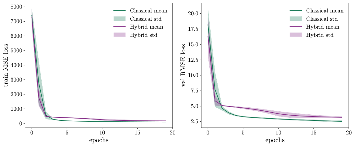
Figure 3 shows the training MSE loss and the validation RMSE over the twenty epochs, as mean ± standard deviation across the ten seeds, for the HQRNN and its matched-parameter classical RNN (RNN-20-16-4-8-16). Both models converge rapidly: the training loss and the validation RMSE drop sharply within the first few epochs and are essentially flat well before epoch 20, confirming that the fixed twenty-epoch schedule is sufficient on FD001 and that neither model is undertrained. Consistent with Table 2, the classical RNN reaches a marginally lower validation RMSE while the HQRNN generalises better on the held-out test engines; note that the validation RMSE is evaluated on overlapping windows and is therefore optimistic relative to the engine-level test metric.

We profiled the training and inference cost of every model on CPU, using the same PennyLane lightning.qubit state-vector backend and adjoint gradients as in training (i.e., noiseless simulation). Per-epoch training times are obtained by timing individual 128-sample batches and scaling by the 111 batches of a full FD001 epoch; every figure is a mean over five repetitions.

Table 3. Computational cost on CPU (PennyLane lightning.qubit, noiseless state-vector simulation). Training and inference figures are mean ± standard deviation over five repetitions (warm-up excluded); the classical models’ timing variability rounds below the displayed precision. Per-epoch training times are extrapolated from the measured per-batch times (128-sample batches, 111 batches per FD001 epoch); the full-schedule (20-epoch) times quoted in the text follow by multiplication. “Infer” is the mean inference time per test window and “Peak mem” the maximum resident set size. Each HQRNN forward pass evaluates 360 four-qubit circuits per window ($\approx 5.1\times {10}^6$ per training epoch); the classical models use none.

Model	Params	Train (s/epoch)	Infer (ms/win)	Peak Mem (GB)
HQRNN (Z_basic_Y)	6793	$4189\pm 22$	$242\pm 2$	$2.3$
RNN-32-16-8-16-32	14,609	$2.01\pm 0.06$	$0.047\pm 0.000$	$0.49$
RNN-20-16-4-8-16	6793	$2.00\pm 0.06$	$0.049\pm 0.000$	$0.49$
RNN-16-8-4-8-16	4233	$1.50\pm 0.01$	$0.050\pm 0.000$	$0.49$
RNN-8-4-2-4-8	1349	$1.35\pm 0.04$	$0.048\pm 0.000$	$0.50$

summarises the results.

Simulating the quantum circuits dominates the cost. Each HQRNN forward pass evaluates 360 four-qubit circuits (Section 3.1), i.e., about $5.1\times {10}^6$ logical circuit evaluations per epoch over the $14,184$ training windows. These evaluations are not run one at a time: the 128-sample batch is processed together through PennyLane’s parameter broadcasting and the PyTorch interface, so the timings reported here already reflect this batched execution and are not a naive product of the evaluation count and a per-circuit cost. Even so, a single-process training epoch takes $\approx 4.2\times {10}^3$ s, against $\approx 2$ s for the matched-parameter classical RNN: a factor of roughly $2\times {10}^3$. Inference costs $\approx 0.24$ s per engine window versus $\approx 5\times {10}^{-5}$ s classically, and peak resident memory is $\approx 2.3$ GB versus $\approx 0.5$ GB. This overhead comes from classically simulatingthe quantum circuits, not from any intrinsic property of quantum computation. The cost of such simulation grows exponentially with the number of qubits, which is one reason we keep the circuits to four qubits; on real quantum hardware, the per-circuit cost would scale very differently.

Two practical consequences follow. First, the reported experiments used 16-way gloo data parallelism, which reduces the wall-clock time of a full 20-epoch training run to an estimated $\approx 1.5$ h, against $\approx 23$ h single-process (both obtained from the per-epoch time of Table 3). Second, because the circuits use only four qubits, they can be simulated exactly on an ordinary classical computer; the HQRNN can therefore be trained and deployed today without access to a quantum processor.

We therefore state the scope of our claims precisely. The advantage demonstrated in this work is one of parameter efficiency and predictive accuracy: at a matched or smaller weight budget, the HQRNN attains a lower test error than the classical RNN (Section 4). It is not an advantage in computational efficiency. Under present-day classical simulation the HQRNN is about $2\times {10}^3$ times slower to train, about $5\times {10}^3$ times slower per inference, and roughly $5\times$ more memory-intensive than the matched-parameter classical RNN. On modern simulators, therefore, the HQRNN provides no advantage in speed or resource use: the model is more compact in its number of weights and more accurate, but markedly more expensive to run on simulators. Its practical case rests on that compactness in data-scarce regimes and on the prospect of native quantum execution once the hardware matures (Section 6.3).

5. Quantum Circuit Analysis

This section examines the QDI layer used in the QLSTM network through three complementary perspectives: redundancy analysis with ZX calculus, trainability analysis using Fisher information, and expressivity analysis via Fourier-series decomposition.

With one exception, these analyses probe the isolated QDI circuit under random or Gaussian inputs rather than the fully trained HQRNN; the exception is the Fisher-information analysis, which we additionally repeat on the empirical input distribution recorded from the trained models (Section 5.2). They should be read as necessary, but not sufficient, indicators that the circuit is compact, optimisable, and expressive, and they do not, on their own, establish that the empirical improvement in Section 4 originates from a quantum-mechanical effect.

5.1. Redundancy Analysis: ZX Calculus

ZX calculus is a graphical language for representing and simplifying quantum circuits [61,62]. It employs “spider” nodes, enabling the analysis and optimisation of quantum gates through well-defined algebraic rewriting rules. By using ZX techniques, one can in principle reduce the number of parameters and gates in a quantum circuit without changing its overall functionality [63,64].

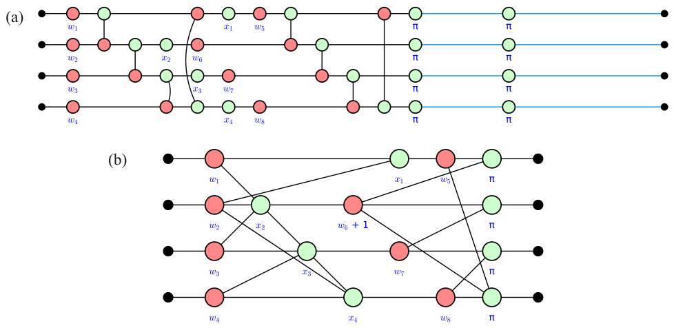
Figure 4 illustrates the original QDI circuit (a) and its ZX-optimised form (b). The primary modifications involve rearranging certain weights and merging CNOT gates with them. Under the rewrite rules we applied, all 8 parameters of the original circuit remain essential and no further parameter reduction was found without altering the circuit’s behaviour. The QDI structure thus appears ZX-irreducible under these rules, consistent with efficient parameter usage.

5.2. Trainability: Fisher Information

In supervised machine learning, a model $h_{\theta }(\hat{x})$ is trained on a labelled dataset $\mathcal{D}={\left\{(x_i,y_i)\right\}}_{i=1}^N$, where the model parameters $\theta =({\theta }^1,{\theta }^2,\dots ,{\theta }^n)$ define a conditional probability distribution $p(y\mid x,\theta )$ that can also be expressed via the joint distribution $p(x,y\mid \theta )$ as $p(y\mid x,\theta )=p(x,y\mid \theta )/p(x)$. The set of all such distributions for different $\theta$ forms a manifold $\mathcal{M}=\{p(y\mid x,\theta ),\theta \in \mathrm{\Theta }\}$.

Defining the score function as $s(\theta )={\nabla }_{\theta }\log p(y\mid x,\theta )$, the Fisher Information Matrix (FIM) is the covariance of the score [65]:

$$F(\theta )=\mathrm{Cov}\left[s(\theta )\right]={\mathbb{E}}_{p(x,y\mid \theta )}\left[s(\theta )s{(\theta )}^{\top }\right].$$

(8)

In practice the FIM is approximated by the sample average. Moreover, the “volume” of the manifold $\mathcal{M}$ can be evaluated as $V\propto {\int }_{\mathrm{\Theta }}\sqrt{\det F(\theta )}d\theta$, whose logarithm corresponds to the effective dimension introduced in [66] and serves as a measure of model complexity.

A significant motivation for analysing the FIM is its connection to the barren-plateau phenomenon, in which training gradients vanish exponentially with system size and thereby obstruct optimisation [67]. Barren plateaus are therefore detrimental to learning, and a trainable circuit is one that avoids them. In terms of the FIM, a large fraction of near-zero eigenvalues is the signature of a barren plateau and hence of poor trainability, whereas an eigenvalue spectrum spread away from zero indicates informative gradients and favourable trainability [40]. A well-conditioned circuit is thus expected to show a negligible fraction of near-zero eigenvalues.

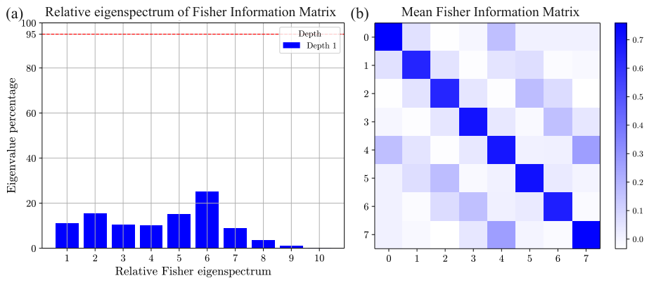
Following [40,68], we compute the FIM of the QDI circuit on a Gaussian dataset $x\sim \mathcal{N}(0,1)$. By averaging over x and y, one obtains the mean FIM. Figure 5a shows the normalised histogram of FIM eigenvalues; the eigenvalues are well-distributed with no significant concentration near zero. In Figure 5b, the diagonal structure in the averaged FIM indicates that gradients are approximately evenly allocated across parameters, while minimal off-diagonal elements suggest weak cross-parameter entanglement and straightforward optimisation.

These results indicate that, on this synthetic input distribution, the isolated QDI circuit shows no signature of barren plateaus, a necessary (though not sufficient) condition for trainability on the RUL prediction task.

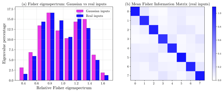
The Gaussian dataset above characterises the QDI architecture in isolation. Because each QDI sits inside the QLSTM cell, however, its actual input is the four-dimensional gate input projection $a_t^{\gamma }$ of Equation (1), not a raw sensor reading or a standard normal. To test whether the trainability indication survives on realistic inputs, we recomputed the FIM on the empirical distribution of $a_t^{\gamma }$. Concretely, we ran the ten trained HQRNNs over C-MAPSS windows and recorded, via forward hooks on the twelve circuits (three QLSTM layers × four gates), the $360,000$ input vectors actually presented to the QDI layers; we then repeated the Fisher analysis of Equation (8) drawing the inputs from this empirical distribution instead of from $\mathcal{N}(0,1)$. The recorded inputs are centred near zero with standard deviation $1.26$ and range $[-8.6,11.1]$, a scale comparable to $\mathcal{N}(0,1)$ but with noticeably heavier tails.

As shown in Figure 6, using the real inputs leaves the FIM eigenvalue spectrum essentially unchanged: it overlaps the synthetic-Gaussian spectrum almost exactly, the smallest eigenvalue remains $\approx 0.33$ with no mass near zero, and the averaged FIM retains the diagonal structure of Figure 5b. The same behaviour is observed when the random circuit weights are replaced by the trained weights (a local FIM evaluated at the learned solution). We therefore find no barren-plateau signature under the real operating distribution, indicating that the trainability reading above is not an artefact of the synthetic Gaussian assumption. As with the other circuit diagnostics, this remains supporting rather than conclusive evidence and characterises the isolated circuit.

5.3. Expressivity: Fourier Series

Quantum neural networks employing angle-based encoding can be interpreted through the lens of truncated Fourier series [59,69,70]. The circuit’s capacity to represent a function $f(\theta ,x)$ can be expressed as a multi-dimensional Fourier series whose degree of truncation depends on the number of encoding repetitions [71]. For two encoded features, each repeated once, the function becomes

$$f(\theta ,x)=\langle \psi (\theta ,x)\mid M\mid \psi (\theta ,x)\rangle ={\displaystyle \sum _{n=-1}^1}{\displaystyle \sum _{m=-1}^1}{c}_{nm}(\theta )e^{i(n{x}_1+m{x}_2)},$$

(9)

where $|\psi (\theta ,x)\rangle$ is the quantum state after all parameterised operations, M is the observable, and $c_{nm}$ are complex coefficients determined by the circuit parameters. Although the maximal Fourier frequencies are limited by circuit depth, they can be sufficient to capture higher-order correlations in real-world datasets. A higher number of non-zero coefficients represents more complex dependencies the model can detect.

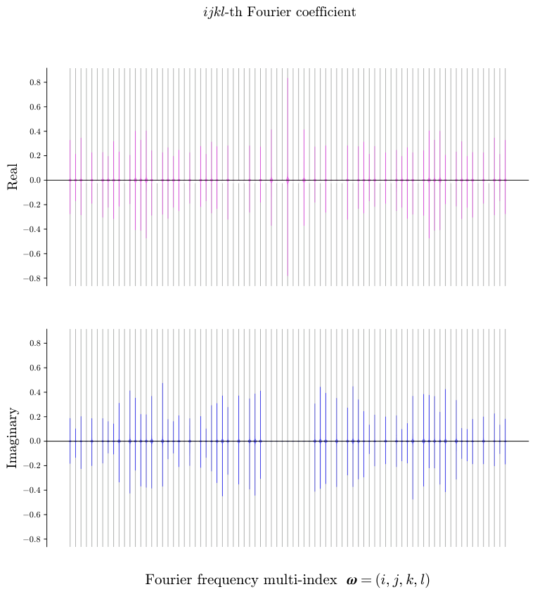
In the QDI circuit we assess Fourier accessibility by encoding four features, each appearing only once. Randomly initialising the circuit parameters with 1000 samples, we compute the real and imaginary parts of the resulting Fourier spectrum, as shown in Figure 7. Out of 161 possible frequency components, 109 have non-negligible amplitude ($\sim 67\%$), indicating that a large portion of the circuit’s Fourier space is accessible under random initialisation. The QDI layer therefore has access to a broad Fourier spectrum, a property that can be advantageous when representing complex high-dimensional signals.

5.4. Summary of Circuit Analysis

Taken together, the three analyses give a consistent picture of the QDI circuit. First, the ZX-based rewriting shows that the circuit is compactly parameterised: no parameter can be removed under the rules we applied. Second, the Fisher-information analysis reveals no barren-plateau signature, neither on the synthetic Gaussian inputs nor, importantly, on the empirical C-MAPSS input distribution recorded from the trained HQRNNs (Section 5.2), which is consistent with good optimisability. Third, the Fourier analysis shows that a substantial portion of the circuit’s Fourier spectrum is accessible under random initialisation, indicating strong expressivity. In this way the three diagnostics jointly characterise the QDI block as compact, optimisable, and expressive. We stress, however, that they remain necessary rather than sufficient indicators: even with the real-input Fisher result, they describe the circuit in near-isolation and should be read as supporting rather than conclusive evidence that the empirical gains reported in Section 4 have a specifically quantum-mechanical origin.

6. Discussion

The central empirical result of this study is that the HQRNN attains a lower test error than its classical recurrent counterparts on C-MAPSS FD001 while using no more trainable parameters. Crucially, the improvement holds against both classical baseline families of Section 4: the RNN that reuses the HQRNN’s layer widths (and therefore carries more parameters) and the RNN whose widths are reduced to match the HQRNN’s parameter count. Averaged over ten seeds, the HQRNN improves mean test RMSE and MAE by about $5\%$ at an equal or smaller parameter budget. We read this as evidence of parameter efficiency: replacing each gate’s linear map with a Quantum Depth-Infused circuit acts as a useful inductive bias, favouring smooth, Fourier-rich mappings that resist overfitting when run-to-failure trajectories are scarce, rather than as mere added capacity. The circuit-level analyses of Section 5 are consistent with this reading: the QDI circuit is compactly parameterised (ZX calculus), shows none of the near-zero Fisher spectrum associated with barren plateaus, and can access a broad band of frequencies (Fourier). As we stress below, however, these analyses are supporting rather than conclusive evidence that the gain has a specifically quantum-mechanical origin.

Set against this advantage is a concrete practical limitation. At present the QDI circuits must be simulated classically, and that simulation is far slower and more memory-intensive than running the matched classical RNN (Section 4): the gain is one of parameter efficiency and accuracy, not of computational cost on today’s hardware.

6.1. Comparison with Prior Work

In comparison with classical machine-learning models (Random Forest, LASSO regression, etc.) and simple ANN models (MLP, CNN, LSTM) on this task, the proposed HQRNN model shows the best performance in terms of RMSE (

Table 4. Comparison of the proposed HQRNN model with classical ML models and simple neural-network models on the C-MAPSS FD001 test set. Best RMSE score is in bold.

Type	Method	RMSE
Classical ML	RF [4]	$17.91$
	LASSO [4]	$19.74$
	SVM [4]	$40.72$
	KNR [4]	$20.46$
	GB [4]	$15.67$
ANN	MLP [4]	$16.78$
	CNN [44]	$18.45$
	LSTM [45]	$16.14$
Proposed	HQRNN	$\mathbf{15.46}$

).

However, to achieve state-of-the-art results, ensembles or combinations of neural-network models with sophisticated feature preprocessing are required (

Table 5. Comparison of the proposed HQRNN model with joint deep-learning models on the C-MAPSS FD001 test set. Best RMSE score is in bold.

Method	RMSE
Transformer + TCNN [46]	$12.31$
CNN + LSTM [72]	$16.16$
LSTM + FCLCNN [49]	$11.17$
BLS + TCN [48]	$12.08$
Auto-RUL + LSTM [50]	$\mathbf{7.78}$
HQRNN (proposed)	$15.46$

). For example, the “Auto-RUL + LSTM” model [50] uses a refined degradation model to assign RUL target labels, whereas the present work uses the simple piecewise-linear degradation. It is therefore expected that the joint models in Table 5 outperform our raw HQRNN. This positioning suggests that the proposed model is best used not only on its own but also as a component within complex prognostics pipelines, e.g., as a quantum-enhanced recurrent block within transformer- or attention-based joint architectures, to further improve their performance.

6.2. Implications for Prognostics Pipelines

The empirical and analytical results have several practical implications for prognostics and health management (PHM):

• Parameter efficiency under data scarcity. The HQRNN matches or beats classical LSTMs with up to $\sim 2\times$ fewer parameters, which is attractive for fleets where only a small number of full run-to-failure trajectories are available.
• Component for hybrid pipelines. HQRNN can be inserted into existing prognostics pipelines as a drop-in replacement for an LSTM block, without requiring quantum hardware at inference: the QLSTM layers can be simulated on classical hardware for the small circuit sizes considered here, while still providing the inductive bias of a Fourier-rich feature extractor.
• Robustness to short observation windows. The ability to learn high-frequency components is particularly valuable when only short segments of sensor history are available, a common situation in operational aviation maintenance.

6.3. Requirements and Roadmap for Noisy Quantum Hardware

All results reported above were obtained with ideal, noiseless state-vector simulation (PennyLane lightning.qubit); the QLSTM circuits were not executed on physical hardware or under a device noise model. Because this scope choice bears directly on how the present gains would translate to a quantum processor, we make the hardware requirements, the expected noise level, and a realistic development path explicit in this subsection. A quantitative evaluation on noisy intermediate-scale quantum (NISQ) hardware [21,73] remains the subject of dedicated follow-up work; the estimates below are intended to delimit that effort rather than to substitute for it.

• Each QDI block acts on four qubits and consists of two basic-entangler layers surrounding a single angle-embedding layer (Section 3.1). Being compiled to elementary gates amounts to twelve single-qubit rotations (four $R_x$ in each of the two entangling layers plus four $R_z$ encoding rotations), eight two-qubit CNOT gates (four per entangling layer), and a four-qubit Pauli-Y readout, giving a two-qubit-gate depth of two. A single forward pass over one length-30 window evaluates 360 such circuits (Section 4), but each individual circuit is shallow.
• To first order, the probability that a circuit runs without any error is ${\prod }_g(1-{\epsilon }_g)$, where the product runs over every gate and measurement g in the circuit and ${\epsilon }_g$ is the error probability (infidelity) of that operation. The corresponding total error, $1-{\prod }_g(1-{\epsilon }_g)\approx {\sum }_g{\epsilon }_g$, therefore grows roughly linearly with the number of operations; and because two-qubit gates and measurements are typically one to two orders of magnitude noisier than single-qubit gates, it is dominated by the eight CNOTs and the four-qubit readout [73,74]. Inserting representative present-day superconducting error rates (single-qubit-gate error ${\epsilon }_1\sim {10}^{-4}$, two-qubit-gate error ${\epsilon }_2\sim {10}^{-3}$–${10}^{-2}$, and per-qubit readout error ${\epsilon }_{\mathrm{ro}}\sim {10}^{-2}$), the eight CNOTs contribute $8{\epsilon }_2\approx 1$–$8\%$ and the four-qubit readout $4{\epsilon }_{\mathrm{ro}}\approx 4\%$, while the twelve single-qubit rotations add well under $1\%$. The estimated total is thus of order 5–$15\%$ per circuit execution, the upper end corresponding to median rather than best-in-class calibration. This is small enough that the shallow QDI circuit is a plausible near-term hardware target, yet large enough that error mitigation would be needed before the sampled expectation values could support quantitative RUL predictions. The deliberate choice of only four qubits and unit depth (Section 3.1) is what keeps this budget, and hence the noise, low. Moderate noise levels are, moreover, not necessarily detrimental: appropriately characterised hardware noise can act as an implicit regulariser during quantum-network training [75].
• Turning the same budget around yields concrete hardware targets. Since the eight CNOTs contribute $\approx 8{\epsilon }_2$, keeping their aggregate error below $\sim 5\%$ requires ${\epsilon }_2\lesssim 5\%/8\approx 6\times {10}^{-3}$, a two-qubit-gate fidelity of about $99.4\%$ or better; keeping the four-qubit readout error comparably low ($4{\epsilon }_{\mathrm{ro}}\lesssim 4\%$) requires a readout fidelity above $\sim 99\%$. These targets are already met by the best current hardware: leading superconducting and trapped-ion processors report two-qubit-gate fidelities of $\approx 99.9\%$ (Google’s Willow [76]) and $\approx 99.8\%$ (Quantinuum’s trapped-ion system [77]), with readout fidelities around $99.5\%$, although median rather than best-in-class devices remain somewhat below them. A circuit as shallow as ours is therefore well within reach once error mitigation [74,78] is applied. As for connectivity, the basic-entangler layers couple the four qubits in a CNOT ring $0-1-2-3-0$. On a linear nearest-neighbour chain the three chain links ($0-1$, $1-2$, $2-3$) are native and only the ring-closing $3-0$ link needs an added SWAP; IBM’s heavy-hexagonal lattice [79], whose qubits have at most three neighbours and which contains no four-qubit loops, embeds the four qubits along a path with the same single-SWAP overhead; and trapped-ion processors with all-to-all connectivity [77] realise the ring directly. In every case the connectivity demand of a four-qubit circuit is modest and well within existing device topologies.
• On hardware each circuit returns sampledexpectation values rather than exact ones, with statistical error scaling as $1/\sqrt{N_{\mathrm{shots}}}$. Because a Pauli expectation value on $[-1,1]$ has variance at most one, resolving it to a precision of $\sim {10}^{-2}$ needs $N_{\mathrm{shots}}\sim {({10}^{-2})}^{-2}={10}^4$ shots per circuit; across the 360 circuits of one window this is about $3.6\times {10}^6$ measurements. This sampling cost is distinct from, and additional to, the classical-simulation cost reported in Table 3, and error-mitigation schemes such as zero-noise extrapolation or probabilistic error cancellation [74,78] multiply it further in exchange for reduced bias. Encoding strategies designed explicitly around finite-shot statistics, such as shot-based quantum encoding [80], offer a complementary route to reducing this measurement overhead.
• We therefore envisage a three-stage path to hardware deployment. In the near term, the shallow four-qubit circuits studied here are already within reach of noisy superconducting and trapped-ion devices when combined with error mitigation: utility-scale experiments have extracted accurate expectation values from $\sim 100$-qubit processors running circuits substantially larger than ours [81]. A concrete first step is a noise-aware study (device-calibrated noise models with finite shots, followed by execution on a small physical device), together with noise-robust training strategies [41]. In the medium term, the first below-threshold demonstrations of quantum error correction [76] point towards early logical qubits that would relax the per-gate error ceiling. In the long term, fault-tolerant execution would remove the depth and gate-count constraints altogether, enabling deeper and wider QDI circuits. Establishing where along this path a genuine quantum advantage emerges, and whether the parameter-efficiency gains reported here survive realistic noise and finite sampling, is the central question we leave for future work.

6.4. Limitations and Future Work

Several limitations should be noted. First, the model is evaluated only on the FD001 subset of C-MAPSS; the more challenging FD002–FD004 subsets, which include multiple operating conditions and fault modes, were not considered and remain an important target for future work. Second, the present analysis assumes ideal noiseless simulation of the quantum circuit; quantitative evaluation on noisy intermediate-scale quantum (NISQ) hardware is left for follow-up work. Third, the piecewise-linear degradation model used here is widely adopted but coarse; integrating the HQRNN with the auto-RUL labelling approach [50] or with attention-aware joint architectures [46,47] is a natural next step that may close the gap to the joint-model state-of-the-art.

Looking further ahead, several research directions arise from this study. One is to integrate quantum modules into established forecasting algorithms such as random forests or gradient boosting, where quantum layers can serve as advanced feature encoders. Transformer-based approaches such as TabPFN [82] or Chronos [83] could likewise benefit from quantum enhancements, potentially improving their ability to model complex temporal dependencies. As quantum hardware evolves, adaptive strategies that dynamically vary the circuit size or depth could manage the trade-off between representational capacity and trainability.

7. Conclusions

Reliable remaining-useful-life prediction from short, noisy, and scarce run-to-failure records is a persistent obstacle in prognostics and health management. This study shows that a hybrid quantum–classical recurrent model can address this regime with a markedly smaller parameter budget than its purely classical counterpart: our Hybrid Quantum Recurrent Neural Network, which replaces the linear transformation in each LSTM gate with a Quantum Depth-Infused circuit, matches or exceeds equally sized classical LSTM baselines, improving average RMSE and MAE by about $5\%$ at a matched parameter count on the NASA C-MAPSS FD001 benchmark.

This work makes four core contributions. First, it introduces a hybrid quantum recurrent architecture in which a Quantum Depth-Infused circuit replaces the linear transformation inside every LSTM gate, and then it applies it to turbofan-engine RUL prediction. Second, it establishes a fair, matched-parameter benchmark on C-MAPSS FD001 with statistical-significance testing across ten seeds, showing that the HQRNN generalises better than classical recurrent baselines of equal or larger size. Third, it characterises the quantum gate at the circuit level (redundancy via ZX calculus, trainability via the Fisher information spectrum, and expressivity via the Fourier decomposition) to explain why so compact a circuit trains stably and generalises well. Fourth, it quantifies the computational cost of the approach and sets out the gate-fidelity, connectivity, finite-shot, and error-mitigation requirements for eventual deployment on noisy quantum hardware rather than leaving hardware feasibility unspecified.

Three broader implications follow. First, the result reinforces parameter efficiency as the practically relevant advantage of hybrid quantum models in data-scarce settings, where the number of full degradation trajectories, not compute, is the binding constraint. Second, because the QLSTM is a drop-in replacement for a classical recurrent block and, at the small circuit sizes used here, is efficiently simulable on classical hardware, it can be incorporated as a component within the transformer- and attention-based joint pipelines that define the current state of the art rather than competing with them as a stand-alone predictor. Third, the accompanying circuit-level analysis (ZX calculus, Fisher information, and Fourier expressivity) provides supporting evidence that the chosen QDI circuit is compact, trainable, and expressive, offering design guidance for quantum-enhanced sequence models beyond this specific task.

We emphasise that advanced joint deep-learning architectures still outperform a stand-alone HQRNN, and that the empirical gains reported here reflect parameter efficiency rather than a demonstrated quantum-mechanical mechanism. Establishing when and why hybrid recurrent modules help to extend the study to the harder FD002–FD004 subsets and to noisy hardware and integrating the HQRNN into joint prognostics pipelines are the natural next steps towards practical quantum-enhanced predictive maintenance.

References

1. Si, X.S.; Wang, W.; Hu, C.H.; Zhou, D.H. Remaining useful life estimation–a review on the statistical data driven approaches. Eur. J. Oper. Res. 2011, 213, 1–14. [Google Scholar] [CrossRef]
2. Lee, J.; Wu, F.; Zhao, W.; Ghaffari, M.; Liao, L.; Siegel, D. Prognostics and health management design for rotary machinery systems—Reviews, methodology and applications. Mech. Syst. Signal Process. 2014, 42, 314–334. [Google Scholar] [CrossRef]
3. Berghout, T.; Benbouzid, M. A systematic guide for predicting remaining useful life with machine learning. Electronics 2022, 11, 1125. [Google Scholar] [CrossRef]
4. Zhang, C.; Lim, P.; Qin, A.K.; Tan, K.C. Multiobjective deep belief networks ensemble for remaining useful life estimation in prognostics. IEEE Trans. Neural Netw. Learn. Syst. 2016, 28, 2306–2318. [Google Scholar] [PubMed]
5. Kang, Z.; Catal, C.; Tekinerdogan, B. Remaining useful life (RUL) prediction of equipment in production lines using artificial neural networks. Sensors 2021, 21, 932. [Google Scholar] [CrossRef] [PubMed]
6. Huang, C.G.; Huang, H.Z.; Li, Y.F. A bidirectional LSTM prognostics method under multiple operational conditions. IEEE Trans. Ind. Electron. 2019, 66, 8792–8802. [Google Scholar] [CrossRef]
7. Ferreira, C.; Gonçalves, G. Remaining Useful Life prediction and challenges: A literature review on the use of Machine Learning Methods. J. Manuf. Syst. 2022, 63, 550–562. [Google Scholar] [CrossRef]
8. Box, G.E.; Jenkins, G.M.; Reinsel, G.C.; Ljung, G.M. Time Series Analysis: Forecasting and Control; John Wiley & Sons: Hoboken, NJ, USA, 2015. [Google Scholar]
9. Shumway, R.H.; Stoffer, D.S.; Stoffer, D.S. Time Series Analysis and Its Applications; Springer: Berlin/Heidelberg, Germany, 2000; Volume 3. [Google Scholar]
10. Zhang, G.P. Time series forecasting using a hybrid ARIMA and neural network model. Neurocomputing 2003, 50, 159–175. [Google Scholar] [CrossRef]
11. Hochreiter, S.; Schmidhuber, J. Long short-term memory. Neural Comput. 1997, 9, 1735–1780. [Google Scholar] [CrossRef] [PubMed]
12. Gers, F.A.; Schmidhuber, J.; Cummins, F. Learning to forget: Continual prediction with LSTM. Neural Comput. 2000, 12, 2451–2471. [Google Scholar] [CrossRef] [PubMed]
13. Graves, A.; Mohamed, A.R.; Hinton, G. Speech recognition with deep recurrent neural networks. In Proceedings of the 2013 IEEE International Conference on Acoustics, Speech and Signal Processing; IEEE: Piscataway, NJ, USA, 2013; pp. 6645–6649. [Google Scholar]
14. Sak, H.; Senior, A.W.; Beaufays, F. Long short-term memory recurrent neural network architectures for large scale acoustic modeling. In Proceedings of the Interspeech 2014, Singapore, 14–18 September 2014; ISCA: Baixas, France, 2014; pp. 338–342. [Google Scholar]
15. Al-Selwi, S.; Hassan, M.F.; Jadid Abdulkadir, S.; Muneer, A.; Sumiea, E.; Alqushaibi, A.; Ragab, M. RNN-LSTM: From applications to modeling techniques and beyond—Systematic review. J. King Saud Univ.-Comput. Inf. Sci. 2024, 36, 102068. [Google Scholar] [CrossRef]
16. Bishop, C.M. Pattern Recognition and Machine Learning; Information Science and Statistics; Springer: New York, NY, USA, 2006. [Google Scholar]
17. Goodfellow, I.; Bengio, Y.; Courville, A.; Bengio, Y. Deep Learning; MIT Press: Cambridge, MA, USA, 2016; Volume 1. [Google Scholar]
18. Nielsen, M.A.; Chuang, I.L. Quantum Computation and Quantum Information; Cambridge University Press: Cambridge, UK, 2010. [Google Scholar]
19. Biamonte, J.; Wittek, P.; Pancotti, N.; Rebentrost, P.; Wiebe, N.; Lloyd, S. Quantum machine learning. Nature 2017, 549, 195–202. [Google Scholar] [CrossRef] [PubMed]
20. Montanaro, A. Quantum algorithms: An overview. npj Quantum Inf. 2016, 2, 15023. [Google Scholar] [CrossRef]
21. Preskill, J. Quantum computing in the NISQ era and beyond. Quantum 2018, 2, 79. [Google Scholar] [CrossRef]
22. Rebentrost, P.; Mohseni, M.; Lloyd, S. Quantum support vector machine for big data classification. Phys. Rev. Lett. 2014, 113, 130503. [Google Scholar] [CrossRef] [PubMed]
23. Ciliberto, C.; Herbster, M.; Ialongo, A.D.; Pontil, M.; Rocchetto, A.; Severini, S.; Wossnig, L. Quantum machine learning: A classical perspective. Proc. R. Soc. A Math. Phys. Eng. Sci. 2018, 474, 20170551. [Google Scholar] [CrossRef] [PubMed]
24. Schuld, M.; Petruccione, F. Supervised Learning with Quantum Computers; Quantum Science and Technology; Springer: Cham, Switzerland, 2018. [Google Scholar]
25. Cao, Y.; Guerreschi, G.G.; Aspuru-Guzik, A. Quantum neuron: An elementary building block for machine learning on quantum computers. arXiv 2017, arXiv:1711.11240. [Google Scholar]
26. Alharbi, M.; Ahmad, S. Deep Revamped Quantum Convolutional Neural Network on Fashion MNIST Dataset. Data Metadata 2024, 3, 358–368. [Google Scholar] [CrossRef]
27. Havlíček, V.; Córcoles, A.D.; Temme, K.; Harrow, A.W.; Kandala, A.; Chow, J.M.; Gambetta, J.M. Supervised learning with quantum-enhanced feature spaces. Nature 2019, 567, 209–212. [Google Scholar] [CrossRef] [PubMed]
28. Schuld, M.; Killoran, N. Quantum machine learning in feature Hilbert spaces. Phys. Rev. Lett. 2019, 122, 040504. [Google Scholar] [CrossRef] [PubMed]
29. Emmanoulopoulos, D.; Dimoska, S. Quantum machine learning in finance: Time series forecasting. arXiv 2022, arXiv:2202.00599. [Google Scholar]
30. Sagingalieva, A.; Komornyik, S.; Senokosov, A.; Joshi, A.; Mansell, C.; Tsurkan, O.; Pinto, K.; Pflitsch, M.; Melnikov, A. Photovoltaic power forecasting using quantum machine learning. Sol. Energy 2025, 302, 114016. [Google Scholar] [CrossRef]
31. Kordzanganeh, M.; Sekatski, P.; Fedichkin, L.; Melnikov, A. An exponentially-growing family of universal quantum circuits. Mach. Learn. Sci. Technol. 2023, 4, 035036. [Google Scholar] [CrossRef]
32. Arthur, D. A hybrid quantum-classical neural network architecture for binary classification. arXiv 2022, arXiv:2201.01820. [Google Scholar]
33. Haboury, N.; Kordzanganeh, M.; Melnikov, A.; Sekatski, P. Information plane and compression-gnostic feedback in quantum machine learning. arXiv 2024, arXiv:2411.02313. [Google Scholar]
34. Bischof, L.; Teodoropol, S.; Füchslin, R.M.; Stockinger, K. Hybrid quantum neural networks show strongly reduced need for free parameters in entity matching. Sci. Rep. 2025, 15, 4318. [Google Scholar] [CrossRef] [PubMed]
35. Sun, Y.; Li, D.; Xiang, Q.; Yuan, Y.; Hu, Z.; Hua, X.; Jiang, Y.; Zhu, Y.; Fu, Y. Scalable quantum convolutional neural network for image classification. Phys. A Stat. Mech. Its Appl. 2025, 657, 130226. [Google Scholar] [CrossRef]
36. Patapovich, V.; Periyasamy, M.; Kordzanganeh, M.; Melnikov, A. Superposed parameterised quantum circuits. arXiv 2025, arXiv:2506.08749. [Google Scholar]
37. Broughton, M.; Verdon, G.; McCourt, T.; Martinez, A.J.; Yoo, J.H.; Isakov, S.V.; Massey, P.; Halavati, R.; Niu, M.Y.; Zlokapa, A.; et al. Tensorflow quantum: A software framework for quantum machine learning. arXiv 2020, arXiv:2003.02989. [Google Scholar]
38. Haboury, N.; Kordzanganeh, M.; Schmitt, S.; Joshi, A.; Tokarev, I.; Abdallah, L.; Kurkin, A.; Kyriacou, B.; Melnikov, A. A supervised hybrid quantum machine learning solution to the emergency escape routing problem. arXiv 2023, arXiv:2307.15682. [Google Scholar]
39. Sagingalieva, A.; Lusnig, L.; Cavalli, F.; Melnikov, A. Hybrid quantum neural networks for computer-aided sex diagnosis in forensic and physical anthropology. Inform. Med. Unlocked 2025, 58, 101682. [Google Scholar] [CrossRef]
40. Abbas, A.; Sutter, D.; Zoufal, C.; Lucchi, A.; Figalli, A.; Woerner, S. The power of quantum neural networks. Nat. Comput. Sci. 2021, 1, 403–409. [Google Scholar] [CrossRef] [PubMed]
41. Berberich, J.; Fink, D.; Pranjić, D.; Tutschku, C.; Holm, C. Training robust and generalizable quantum models. Phys. Rev. Res. 2024, 6, 043326. [Google Scholar] [CrossRef]
42. Saxena, A.; Goebel, K.; Simon, D.; Eklund, N. Damage propagation modeling for aircraft engine run-to-failure simulation. In 2008 International Conference on Prognostics and Health Management; IEEE: Piscataway, NJ, USA, 2008; pp. 1–9. [Google Scholar]
43. Saxena, A.; Goebel, K. Turbofan engine degradation simulation data set. NASA Ames Progn. Data Repos. 2008, 18, 878–887. [Google Scholar]
44. Sateesh Babu, G.; Zhao, P.; Li, X.L. Deep convolutional neural network based regression approach for estimation of remaining useful life. In Proceedings of the Database Systems for Advanced Applications: 21st International Conference, DASFAA 2016, Dallas, TX, USA, 16–19 April 2016; proceedings, part i 21; Springer: Berlin/Heidelberg, Germany, 2016; pp. 214–228. [Google Scholar]
45. Zheng, S.; Ristovski, K.; Farahat, A.; Gupta, C. Long short-term memory network for remaining useful life estimation. In Proceedings of the 2017 IEEE international conference on prognostics and health management (ICPHM); IEEE: Piscataway, NJ, USA, 2017; pp. 88–95. [Google Scholar]
46. Wang, H.K.; Cheng, Y.; Song, K. Remaining useful life estimation of aircraft engines using a joint deep learning model based on TCNN and transformer. Comput. Intell. Neurosci. 2021, 2021, 5185938. [Google Scholar] [CrossRef] [PubMed]
47. Deng, S.; Zhou, J. Prediction of remaining useful life of aero-engines based on CNN-LSTM-Attention. Int. J. Comput. Intell. Syst. 2024, 17, 232. [Google Scholar] [CrossRef]
48. Yu, K.; Wang, D.; Li, H. A prediction model for remaining useful life of turbofan engines by fusing broad learning system and temporal convolutional network. In Proceedings of the 2021 8th International Conference on Information, Cybernetics, and Computational Social Systems (ICCSS); IEEE: Piscataway, NJ, USA, 2021; pp. 137–142. [Google Scholar]
49. Peng, C.; Chen, Y.; Chen, Q.; Tang, Z.; Li, L.; Gui, W. A remaining useful life prognosis of turbofan engine using temporal and spatial feature fusion. Sensors 2021, 21, 418. [Google Scholar] [CrossRef] [PubMed]
50. Asif, O.; Haider, S.A.; Naqvi, S.R.; Zaki, J.F.; Kwak, K.S.; Islam, S.R. A deep learning model for remaining useful life prediction of aircraft turbofan engine on C-MAPSS dataset. IEEE Access 2022, 10, 95425–95440. [Google Scholar] [CrossRef]
51. Kurkin, A.; Hegemann, J.; Kordzanganeh, M.; Melnikov, A. Forecasting steam mass flow in power plants using the parallel hybrid network. Eng. Appl. Artif. Intell. 2025, 160, 111912. [Google Scholar] [CrossRef]
52. Laskaris, G.; Morozov, D.; Tarpanov, D.; Seth, A.; Procelewska, J.; Sai Gautam, G.; Sagingalieva, A.; Brasher, R.; Melnikov, A. Multi-objective optimization and quantum hybridization of equivariant deep learning interatomic potentials. Comput. Mater. Sci. 2026, 270, 114742. [Google Scholar] [CrossRef]
53. Lusnig, L.; Sagingalieva, A.; Surmach, M.; Protasevich, T.; Michiu, O.; McLoughlin, J.; Mansell, C.; de’Petris, G.; Bonazza, D.; Zanconati, F.; et al. Hybrid quantum image classification and federated learning for hepatic steatosis diagnosis. Diagnostics 2024, 14, 558. [Google Scholar] [CrossRef] [PubMed]
54. Chen, S.Y.C.; Yoo, S.; Fang, Y.L.L. Quantum long short-term memory. In Proceedings of the Icassp 2022-2022 IEEE International Conference on Acoustics, Speech and Signal Processing (ICASSP); IEEE: Piscataway, NJ, USA, 2022; pp. 8622–8626. [Google Scholar]
55. Sagingalieva, A.; Kordzanganeh, M.; Kenbayev, N.; Kosichkina, D.; Tomashuk, T.; Melnikov, A. Hybrid quantum neural network for drug response prediction. Cancers 2023, 15, 2705. [Google Scholar] [CrossRef] [PubMed]
56. Anoshin, M.; Sagingalieva, A.; Mansell, C.; Zhiganov, D.; Shete, V.; Pflitsch, M.; Melnikov, A. Hybrid quantum cycle generative adversarial network for small molecule generation. IEEE Trans. Quantum Eng. 2024, 5, 2500514. [Google Scholar] [CrossRef]
57. Lopatkin, V.; Sagingalieva, A.; Lusnig, L.; Protasevich, T.; Behnke, B.; Melnikov, A. Quantum hybrid feature selector. EPJ Quantum Technol. 2026, 13, 49. [Google Scholar] [CrossRef]
58. Xu, Z.Q.J.; Zhang, Y.; Xiao, Y. Training behavior of deep neural network in frequency domain. In Proceedings of the Neural Information Processing: 26th International Conference, ICONIP 2019, Sydney, NSW, Australia, 12–15 December 2019; Proceedings, Part I 26; Springer: Berlin/Heidelberg, Germany, 2019; pp. 264–274. [Google Scholar]
59. Schuld, M.; Sweke, R.; Meyer, J.J. Effect of data encoding on the expressive power of variational quantum-machine-learning models. Phys. Rev. A 2021, 103, 032430. [Google Scholar] [CrossRef]
60. Caro, M.C.; Huang, H.Y.; Cerezo, M.; Sharma, K.; Sornborger, A.; Cincio, L.; Coles, P.J. Generalization in quantum machine learning from few training data. Nat. Commun. 2022, 13, 4919. [Google Scholar] [CrossRef] [PubMed]
61. Coecke, B.; Duncan, R. Interacting quantum observables: Categorical algebra and diagrammatics. New J. Phys. 2011, 13, 043016. [Google Scholar] [CrossRef]
62. van de Wetering, J. ZX-calculus for the working quantum computer scientist. arXiv 2020, arXiv:2012.13966. [Google Scholar]
63. Peham, T.; Burgholzer, L.; Wille, R. Equivalence checking of quantum circuits with the ZX-calculus. IEEE J. Emerg. Sel. Top. Circuits Syst. 2022, 12, 662–675. [Google Scholar] [CrossRef]
64. Wang, Q.; Yeung, R.; Koch, M. Differentiating and integrating ZX diagrams with applications to quantum machine learning. Quantum 2024, 8, 1491. [Google Scholar] [CrossRef]
65. Amari, S.i. Natural gradient works efficiently in learning. Neural Comput. 1998, 10, 251–276. [Google Scholar] [CrossRef]
66. Berezniuk, O.; Figalli, A.; Ghigliazza, R.; Musaelian, K. A scale-dependent notion of effective dimension. arXiv 2020, arXiv:2001.10872. [Google Scholar]
67. McClean, J.R.; Boixo, S.; Smelyanskiy, V.N. Barren plateaus in quantum neural network training landscapes. Nat. Commun. 2018, 9, 4812. [Google Scholar] [CrossRef] [PubMed]
68. Araz, J.Y.; Spannowsky, M. Classical versus quantum: Comparing tensor-network-based quantum circuits on Large Hadron Collider data. Phys. Rev. A 2022, 106, 062423. [Google Scholar] [CrossRef]
69. Peters, E.; Schuld, M. Generalization despite overfitting in quantum machine learning models. Quantum 2023, 7, 1210. [Google Scholar] [CrossRef]
70. Atchadé, P.; Larson, K. Fourier Series Weight in Quantum Machine Learning. Adv. Artif. Intell. Mach. Learn. 2024, 4, 1866–1890. [Google Scholar] [CrossRef]
71. Pérez-Salinas, A.; Cervera-Lierta, A.; Gil-Fuster, E.; Latorre, J.I. Data re-uploading for a universal quantum classifier. Quantum 2020, 4, 226. [Google Scholar] [CrossRef]
72. Kong, Z.; Cui, Y.; Xia, Z.; Lv, H. Convolution and long short-term memory hybrid deep neural networks for remaining useful life prognostics. Appl. Sci. 2019, 9, 4156. [Google Scholar] [CrossRef]
73. Bharti, K.; Cervera-Lierta, A.; Kyaw, T.H.; Haug, T.; Alperin-Lea, S.; Anand, A.; Degroote, M.; Heimonen, H.; Kottmann, J.S.; Menke, T.; et al. Noisy intermediate-scale quantum algorithms. Rev. Mod. Phys. 2022, 94, 015004. [Google Scholar] [CrossRef]
74. Cai, Z.; Babbush, R.; Benjamin, S.C.; Endo, S.; Huggins, W.J.; Li, Y.; McClean, J.R.; O’Brien, T.E. Quantum error mitigation. Rev. Mod. Phys. 2023, 95, 045005. [Google Scholar] [CrossRef]
75. Kuzmin, V.; Somogyi, W.; Pankovets, E.; Melnikov, A. Method for noise-induced regularization in quantum neural networks. Adv. Quantum Technol. 2025, 8, e00603. [Google Scholar] [CrossRef]
76. Google Quantum AI and Collaborators. Quantum error correction below the surface code threshold. Nature 2025, 638, 920–926. [Google Scholar] [CrossRef] [PubMed]
77. Moses, S.A.; Baldwin, C.H.; Allman, M.S.; Ancona, R.; Ascarrunz, L.; Barnes, C.; Bartolotta, J.; Bjork, B.; Blanchard, P.; Bohn, M.; et al. A race-track trapped-ion quantum processor. Phys. Rev. X 2023, 13, 041052. [Google Scholar] [CrossRef]
78. Temme, K.; Bravyi, S.; Gambetta, J.M. Error mitigation for short-depth quantum circuits. Phys. Rev. Lett. 2017, 119, 180509. [Google Scholar] [CrossRef] [PubMed]
79. Chamberland, C.; Zhu, G.; Yoder, T.J.; Hertzberg, J.B.; Cross, A.W. Topological and subsystem codes on low-degree graphs with flag qubits. Phys. Rev. X 2020, 10, 011022. [Google Scholar] [CrossRef]
80. Kyriacou, B.; Patapovich, V.; Periyasamy, M.; Melnikov, A. Shot-based quantum encoding: A data-loading paradigm for quantum neural networks. Adv. Comput. 2026, 1, e70004. [Google Scholar] [CrossRef]
81. Kim, Y.; Eddins, A.; Anand, S.; Wei, K.X.; van den Berg, E.; Rosenblatt, S.; Nayfeh, H.; Wu, Y.; Zaletel, M.; Temme, K.; et al. Evidence for the utility of quantum computing before fault tolerance. Nature 2023, 618, 500–505. [Google Scholar] [CrossRef] [PubMed]
82. Hollmann, N.; Müller, S.; Eggensperger, K.; Hutter, F. Tabpfn: A transformer that solves small tabular classification problems in a second. In Proceedings of the International Conference on Learning Representations (ICLR), Kigali, Rwanda, 1–5 May 2023. [Google Scholar]
83. Ansari, A.F.; Stella, L.; Turkmen, C.; Zhang, X.; Mercado, P.; Shen, H.; Shchur, O.; Rangapuram, S.S.; Arango, S.P.; Kapoor, S.; et al. Chronos: Learning the language of time series. arXiv 2024, arXiv:2403.07815. [Google Scholar]
Figure 1. Remaining useful life (RUL) of engine 2 (FD001) under the linear and piecewise-linear degradation models. Both axes are measured in engine operating cycles but represent complementary quantities: the horizontal axis is the elapsed operating time t (the number of cycles the engine has already run), whereas the vertical axis is the remaining useful life until failure, RUL ( t ) = T life t (here the engine fails at T life = 287 cycles). The dotted line marks the early-RUL threshold: this work adopts the piecewise-linear model, which caps the RUL target at 125 cycles, so that the network is only asked to track the RUL once the engine approaches end of life.
Algorithms 19 00663 g001
Figure 2. (a) HQRNN model pipeline. A data window of size W × 14 is processed through three stacked QLSTM layers followed by classical dense layers, yielding a single RUL value. The dimensions of the QLSTM layers are 32, 16, and 8, while the dense layers transition from 8 × W to 16, 16 to 32, and finally 32 to 1. The ## symbols in the engine-data table denote numeric sensor readings. (b) Structure of the QLSTM layer. Conventional linear transformations are replaced by QDI layers for each of the four LSTM gates (forget, input, update, output). (c) Schematic of the QDI layer used in the QLSTM. Each input feature is encoded via R z gates parameterised by that feature on a four-qubit quantum circuit. The variation part consists of trainable R x rotations and CNOT gates. The blue block repeats n = 1 time. The observable is the Pauli Y matrix.
Algorithms 19 00663 g002
Figure 3. Convergence of the classical RNN (“Classical”) and the HQRNN (“Hybrid”) over the twenty training epochs: training MSE loss (left) and validation RMSE (right), shown as the mean (solid line) ± one standard deviation (shaded band) across the ten seeds. Both curves plateau well before epoch 20, indicating convergence under the fixed-epoch schedule.
Algorithms 19 00663 g003
Figure 4. (a) A QDI layer before applying ZX-based parameter reduction. (b) The ZX-reduced QDI layer structure with rearranged weights. Despite these simplifications, no parameters can be removed without affecting the layer’s functionality.
Algorithms 19 00663 g004
Figure 5. (a) Normalised histogram of the Fisher eigenvalue spectrum. The small number of close-to-zero eigenvalues indicates resilience to the barren-plateau problem [40]. (b) Averaged normalised Fisher Information Matrix. The diagonal pattern indicates that the quantum circuit distributes gradients evenly across trainable parameters; weak anti-diagonal elements imply parameters are approximately independent.
Algorithms 19 00663 g005
Figure 6. Fisher analysis on the empirical C-MAPSS-derived QDI input distribution. (a) FIM eigenvalue spectrum computed with the real circuit inputs overlaid on the synthetic-Gaussian baseline; the two distributions are nearly identical and neither places mass near zero. (b) Averaged normalised FIM for the real inputs, exhibiting the same diagonal structure as Figure 5b. Inputs were captured from the ten trained HQRNNs; the eigenvalue spectrum is unchanged when the trained weights are used in place of random ones.
Algorithms 19 00663 g006
Figure 7. Fourier coefficients of a QDI layer with four input features. The horizontal axis enumerates the Fourier frequency multi-indices ω = ( i , j , k , l ) accessible to the circuit (one vertical line per coefficient), and the two panels show, respectively, the real and imaginary parts of the corresponding complex coefficient c ω ; each coloured bar spans the range that coefficient takes over 1000 random weight samples. The coefficients are amplitudes of the circuit’s [ 1 , 1 ] -valued expectation output and are therefore dimensionless, so the vertical axes carry no physical unit. The prevalence of non-zero coefficients (∼67%) indicates substantial expressivity.
Algorithms 19 00663 g007