An Algorithmic MADM Framework for Risk Assessment Based on Complex Einstein Aggregation Operators

Abstract

Business risk assessment is a critical component of effective decision making, as it requires the systematic evaluation of multiple alternatives under diverse and often uncertain criteria. With the rapid growth of complex and heterogeneous business data, conventional decision making approaches may face difficulties in simultaneously representing incomplete information, uncertainty, and periodic behavior. These challenges highlight the need for flexible and computationally effective algorithmic frameworks capable of supporting structured risk assessment under uncertain and phase-dependent decision information. To address these challenges, this study developed an Einstein aggregation framework for complex single-valued neutrosophic soft sets (CSvNSSs). This research introduced neutrosophic Einstein weighted average and neutrosophic Einstein weighted geometric aggregation operators to enable nonlinear aggregation of uncertain decision information. The proposed framework provides a flexible mechanism for effectively integrating complex, periodic, and incomplete information in risk assessment and decision-making problems. Fundamental properties of the proposed operators are established to verify their mathematical consistency and applicability. Subsequently, a risk-aware MADM algorithm is developed to aggregate expert assessments, incorporate attribute weights, and rank competing alternatives under simultaneous data and parametric uncertainty. A hypothetical business-location case study is presented to illustrate the computational applicability of the proposed framework, and additional synthetic decision problems are used to examine numerical scalability and internal consistency. The resulting rankings are further examined through comparative analysis with existing aggregation-based decision-making approaches. Finally, this article is concluded with complete research findings, its limitations and future research direction.

1. Introduction

Multi-attribute decision making (MADM) provides a systematic framework for evaluating and ranking a finite set of alternatives with respect to multiple criteria. In many real-world decision environments, however, the available information is incomplete, imprecise, ambiguous, or subject to conflicting expert judgments. These difficulties become particularly pronounced in risk assessment, where decision makers must simultaneously consider multiple risk factors and make decisions despite uncertainty in both the available data and the evaluation parameters. Consequently, developing mathematical models that can represent and aggregate uncertain information without imposing overly restrictive assumptions has become an important research direction in decision science and computational intelligence [1,2,3,4].

Risk-oriented decision problems frequently involve several interacting attributes, and the assessment of an alternative may not be adequately represented by a single deterministic value. In such environments, experts may express different degrees of support, opposition, and uncertainty toward an alternative. MADM methods based on fuzzy and related uncertainty theories have therefore been extensively investigated to provide flexible mechanisms for representing imprecise decision information [5,6,7,8]. Nevertheless, the effectiveness of an MADM method strongly depends on the underlying information representation and on the aggregation mechanism used to combine the assessments of multiple criteria [9,10,11].

The development of fuzzy set theory provided one of the fundamental mathematical tools for representing uncertainty by assigning a membership degree in the unit interval to each element of the universe [12,13,14]. Intuitionistic fuzzy sets subsequently extended this representation by incorporating membership and non-membership degrees [15]. Although this extension provides additional information, the associated degrees remain subject to a restrictive interrelationship. Picture fuzzy sets further introduced a neutral degree, thereby enabling an additional form of indeterminate assessment [16,17]. Neutrosophic set theory generalized this framework by independently characterizing truth, indeterminacy, and falsity, providing greater flexibility for representing inconsistent and indeterminate information [18,19]. These developments have substantially expanded the capacity of mathematical models to represent uncertainty in decision-making problems.

In parallel with the development of fuzzy and neutrosophic models, soft set theory was introduced as a parameterized mathematical framework for dealing with uncertainty [20]. Unlike conventional set-based representations, soft sets associate information with a collection of parameters, making them particularly suitable for decision problems involving multiple attributes. The integration of fuzzy sets with soft sets led to the development of fuzzy soft sets [21], followed by intuitionistic fuzzy soft sets [22], picture fuzzy soft sets [23], and neutrosophic soft sets [24]. These hybrid structures demonstrate that combining an uncertainty representation with parameterization can provide a more flexible basis for MADM problems.

Despite these developments, real-world information is not always adequately described by real-valued membership degrees. In several decision and information-processing environments, the information may exhibit periodic, cyclic, or phase-dependent characteristics. Complex-valued extensions of fuzzy and soft-set models have therefore been investigated to incorporate both amplitude and phase information. Thirunavukarasu et al. introduced the complex fuzzy soft set by extending fuzzy soft sets from the unit interval to the complex domain [25]. Kumar and Bajaj subsequently developed the complex intuitionistic fuzzy soft set by incorporating complex membership and non-membership information [26]. More recently, Asghar et al. introduced the complex picture fuzzy soft set by incorporating complex membership, non-membership, and neutral information [27]. These developments demonstrate the potential of complex-valued soft-set structures for representing information in which phase or periodic characteristics are relevant.

The complex single-valued neutrosophic soft set (CSvNSS) provides a further extension by combining the parameterization capability of soft sets, the independent representation of truth, indeterminacy, and falsity provided by neutrosophic sets, and the amplitude–phase representation of complex-valued information. The CSvNSS structure was introduced in our previous work [28]. Such a representation can be useful in decision environments where expert assessments contain both uncertainty and phase-related information. Potential applications include cyclical and periodic decision problems, such as seasonal demand assessment, signal classification, communication systems, and other domains in which phase information may carry decision-relevant information.

However, an expressive information representation alone does not guarantee effective decision making. A central issue in CSvNSS-based MADM is the aggregation of multiple complex neutrosophic assessments. The aggregation operator determines how the information associated with different criteria is combined and can therefore substantially influence the resulting scores and rankings. Conventional algebraic and geometric aggregation mechanisms may not provide sufficient flexibility for nonlinear combination of uncertain information. Consequently, the development of suitable aggregation operators for CSvNSS represents an important methodological requirement.

Einstein aggregation operators [29,30,31] provide an alternative family of nonlinear aggregation mechanisms based on an Einstein t-norm and t-conorm. For $\lambda ,\mu \in [0,1]$, the Einstein sum and Einstein product [32,33] are given by:

$$\lambda \oplus \mu ={\displaystyle \frac{\lambda +\mu }{1+\lambda \mu }},\lambda \otimes \mu ={\displaystyle \frac{\lambda \mu }{1+(1-\lambda )(1-\mu )}}.$$

Their nonlinear structure makes them attractive for aggregation in decision-making environments where the interaction between assessments cannot be adequately captured by simple arithmetic operations. Nevertheless, an appropriate extension of these operators to the CSvNSS framework requires careful treatment of the truth, indeterminacy, falsity, amplitude, and phase components while preserving the admissibility conditions of the underlying structure.

1.1. Research Gap and Motivation

The preceding discussion reveals two related gaps in the existing literature. First, although several fuzzy, intuitionistic fuzzy, picture fuzzy, neutrosophic, soft-set, and complex-valued extensions have been developed, the aggregation of complex single-valued neutrosophic soft information remains insufficiently explored. In particular, the simultaneous treatment of parameterized information, independent neutrosophic components, and complex-valued phase information requires aggregation mechanisms specifically designed for this hybrid structure. Second, existing aggregation approaches do not fully exploit the nonlinear behavior of Einstein t-norms and t-conorms within the CSvNSS environment.

These gaps motivate the development of Einstein-based aggregation operators for CSvNSS. The objective is not merely to introduce another aggregation formula, but to establish a mathematically consistent mechanism for combining complex neutrosophic assessments while retaining the structural characteristics of CSvNSS. The proposed framework is subsequently integrated into an MADM procedure for risk assessment, where uncertain assessments from multiple criteria must be aggregated and transformed into a ranking of competing alternatives.

1.2. Contributions

The main contributions of this study are summarized as follows:

• We develop neutrosophic Einstein sum and Einstein product operators for complex single-valued neutrosophic soft sets (CSvNSSs), thereby extending Einstein-type aggregation to a complex neutrosophic parameterized environment.
• Based on the proposed binary operators, we formulate neutrosophic Einstein weighted average aggregation and neutrosophic Einstein weighted geometric aggregation operators for the aggregation of multiple CSvNSS assessments.
• We investigate the fundamental mathematical properties of the proposed aggregation operators and establish their consistency with the underlying CSvNSS structure.
• We develop an Einstein-operator-based MADM procedure for risk assessment that incorporates multiple attributes and uncertain expert evaluations within the CSvNSS framework.
• We demonstrate the applicability of the proposed methodology through a business-location risk assessment problem and compare the resulting rankings with representative existing decision-making approaches.

1.3. Organization of the Paper

The remainder of this paper is organized as follows. Section 2 reviews the preliminary concepts required for the development of the proposed framework. Section 3 introduces the Einstein aggregation operators for complex single-valued neutrosophic soft sets and establishes their relevant properties. Section 4 develops the proposed Einstein-operator-based MADM method and demonstrates its application to a risk assessment problem. Section 5 presents comparative analyses of the proposed framework with existing approaches. Finally, Section 6 concludes the paper and outlines directions for future research.

2. Preliminaries

This section recalls the basic concepts required for the development of the proposed Einstein aggregation operators for complex single-valued neutrosophic soft sets (CSvNSSs). in particular, the concepts of neutrosophic sets, soft sets, and Einstein aggregation operators are briefly reviewed.

Definition 1

(Neutrosophic set, [18]). Let ⊺ be a universal set. A neutrosophic set $\mathbb{NS}$ over ⊺ is characterized by three independent functions ${\mathsf{F}}_{+},{\mathsf{F}}_{-},\mathsf{F}:\mathsf{⊺}\to [0,1]$, representing the truth, falsity, and indeterminacy degrees, respectively. Thus,

$$\mathbb{NS}=\left\{\left(⋏,{\mathsf{F}}_{+}(⋏),{\mathsf{F}}_{-}(⋏),\mathsf{F}(⋏)\right):⋏\in \mathsf{⊺}\right\},$$

where $0\le {\mathsf{F}}_{+}(⋏)+{\mathsf{F}}_{-}(⋏)+\mathsf{F}(⋏)\le 3.$ Unlike intuitionistic and picture fuzzy sets, the three components are not required to satisfy a unit-sum constraint.

Definition 2

(Soft set, [20]). Let ⊺ be a universal set and ⋓ be a set of parameters. A soft set over ⊺ with respect to ⋓ is a pair $(\mathfrak{S},⋓)$, where $\mathfrak{S}:⋓\to \mathfrak{P}\left(\mathsf{⊺}\right),$ and $\mathfrak{P}\left(\mathsf{⊺}\right)$ denotes the power set of ⊺. For each parameter $⋎\in ⋓$, the set $\mathfrak{S}(⋎)$ represents the collection of elements of ⊺ associated with that parameter.

The combination of neutrosophic information with soft-set parameterization provides a suitable framework for representing both uncertain attribute assessments and parameter-dependent information. The combination and complex extension of these frameworks are given in [24,28].

Definition 3

(Einstein aggregation operators, [32,33]). For $\lambda ,\mu \in [0,1]$, the Einstein sum (t-conorm) and Einstein product (t-norm) are defined, respectively, by

$$\lambda \oplus \mu ={\displaystyle \frac{\lambda +\mu }{1+\lambda \mu }},$$

and

$$\lambda \otimes \mu ={\displaystyle \frac{\lambda \mu }{1+(1-\lambda )(1-\mu )}}.$$

These operators provide nonlinear mechanisms for combining information contained in the unit interval.

For convenience, throughout the remainder of this paper, ⊕ and ⊗ denote the Einstein sum and Einstein product, respectively, whereas ${\oplus }_{nes}$ and ${\otimes }_{nep}$ denote their proposed extensions to the CSvNSS framework.

3. Einstein Aggregation Operators for Complex Single-Valued Neutrosophic Soft Sets

This section develops Einstein aggregation operators for complex single-valued neutrosophic soft sets (CSvNSSs). The proposed framework integrates the amplitude and phase information of complex-valued truth, indeterminacy, and falsity degrees within the Einstein t-norm and t-conorm framework. First, the basic representation of a complex single-valued neutrosophic number is recalled. Subsequently, the Einstein sum and product are introduced together with their scalar multiplication and power operations. Based on these operations, the neutrosophic Einstein weighted average aggregation operator (NEWAAO) and neutrosophic Einstein weighted geometric aggregation operator (NEWGAO) are developed in closed form. Several fundamental properties, including closure, commutativity, idempotency, monotonicity, boundedness, and duality, are then established. Finally, a numerical example is presented to demonstrate the computational procedure of the proposed operators.

3.1. Complex Single-Valued Neutrosophic Numbers

A complex single-valued neutrosophic number (CSvNSN) simultaneously represents truth, indeterminacy, and falsity information through complex-valued membership degrees. The modulus and phase of each complex component provide two complementary dimensions of information.

Definition 4 (Complex single-valued neutrosophic number).

A complex single-valued neutrosophic number is expressed as

$$\tilde{\eta }=⟨t{e}^{\iota 2\pi \tau },\iota e^{\iota 2\pi \mu },f{e}^{\iota 2\pi \varphi }⟩,$$

(1)

where $t,\iota ,f,\tau ,\mu ,\varphi \in [0,1]$. Here, t, ι, and f denote the amplitude components corresponding to truth, indeterminacy, and falsity, respectively, whereas τ, μ, and ϕ represent their corresponding normalized phase components.

The use of normalized phase variables in $[0,1]$ allows the actual phase angle to be recovered through multiplication by $2\pi$. Consequently, $e^{\iota 2\pi \tau },e^{\iota 2\pi \mu },e^{\iota 2\pi \varphi }$ belong to the unit circle. For subsequent developments, let ${\tilde{\eta }}_j=⟨t_j{e}^{\iota 2\pi {\tau }_j},{\iota }_j{e}^{\iota 2\pi {\mu }_j},f_j{e}^{\iota 2\pi {\varphi }_j}⟩,$$j=1,2,\dots ,n,$ denote a collection of CSvNSNs.

3.2. Einstein t-Norm and t-Conorm

The Einstein t-conorm and t-norm are, respectively, defined for $x,y\in [0,1]$ as

$$S_E(x,y)={\displaystyle \frac{x+y}{1+xy}},$$

(2)

and

$$T_E(x,y)={\displaystyle \frac{xy}{1+(1-x)(1-y)}}.$$

(3)

Both operators map ${[0,1]}^2$ into $[0,1]$ and are commutative, associative, and monotone in each argument. The generator of the Einstein t-conorm is

$$g_S\left(x\right)=\mathrm{arctanh}\left(x\right)={\displaystyle \frac{1}{2}}\ln \left({\displaystyle \frac{1+x}{1-x}}\right),0<x<1,$$

(4)

with inverse $g_S^{-1}\left(z\right)=\tanh \left(z\right).$ Hence, $S_E(x,y)=g_S^{-1}\left(g_S\left(x\right)+g_S\left(y\right)\right).$ Similarly, the generator of the Einstein t-norm can be written as

$$g_T\left(x\right)=\ln \left({\displaystyle \frac{2-x}{x}}\right),0<x<1,$$

(5)

whose inverse is $g_T^{-1}\left(z\right)={\displaystyle \frac{2}{1+e^z}}.$ Therefore, $T_E(x,y)=g_T^{-1}\left(g_T\left(x\right)+g_T\left(y\right)\right).$ At the boundary points $x=0$ and $x=1$, the generator expressions are interpreted through their limiting values.

3.3. Neutrosophic Einstein Sum and Product

Definition 5 (Neutrosophic Einstein sum).

Let ${\tilde{\eta }}_1$ and ${\tilde{\eta }}_2$ be two CSvNSNs, where

$${\tilde{\eta }}_p=⟨t_p{e}^{\iota 2\pi {\tau }_p},{\iota }_p{e}^{\iota 2\pi {\mu }_p},f_p{e}^{\iota 2\pi {\varphi }_p}⟩,r=1,2.$$

Their neutrosophic Einstein sum is defined by

$${\tilde{\eta }}_1{\oplus }_E{\tilde{\eta }}_2=⟨T^{+}{e}^{\iota 2\pi {\tau }^{+}},i^{-}{e}^{\iota 2\pi {\mu }^{-}},F^{-}{e}^{\iota 2\pi {\varphi }^{-}}⟩,$$

(6)

where $T^{+}=S_E(t_1,t_2),{\tau }^{+}=S_E({\tau }_1,{\tau }_2)$, $i^{-}=T_E({\iota }_1,{\iota }_2),{\mu }^{-}=T_E({\mu }_1,{\mu }_2)$, $F^{-}=T_E(f_1,f_2),{\varphi }^{-}=T_E({\varphi }_1,{\varphi }_2).$

Thus, the truth component is aggregated through the Einstein t-conorm, whereas indeterminacy and falsity are aggregated through the Einstein t-norm. The same transformations are applied to the corresponding normalized phase components.

Definition 6 (Neutrosophic Einstein product).

For two CSvNSNs ${\tilde{\eta }}_1$ and ${\tilde{\eta }}_2$, their neutrosophic Einstein product is defined by

$${\tilde{\eta }}_1{\otimes }_E{\tilde{\eta }}_2=⟨T^{-}{e}^{\iota 2\pi {\tau }^{-}},i^{+}{e}^{\iota 2\pi {\mu }^{+}},F^{+}{e}^{\iota 2\pi {\varphi }^{+}}⟩,$$

(7)

where $T^{-}=T_E(t_1,t_2),{\tau }^{-}=T_E({\tau }_1,{\tau }_2)$, $i^{+}=S_E({\iota }_1,{\iota }_2),{\mu }^{+}=S_E({\mu }_1,{\mu }_2)$, $F^{+}=S_E(f_1,f_2),{\varphi }^{+}=S_E({\varphi }_1,{\varphi }_2).$

3.4. Scalar Multiplication and Power Operations

The generator representation of the Einstein operators naturally leads to scalar transformations.

Definition 7 (Einstein scalar transformations).

For $x\in [0,1]$ and $⊣ >0$, define

$$S_E^{(⊣)}\left(x\right)=g_S^{-1}\left(⊣g_S\left(x\right)\right)=\tanh \left(⊣\mathrm{arctanh}\left(x\right)\right),$$

(8)

and

$$T_E^{(⊣)}\left(x\right)=g_T^{-1}\left(⊣g_T\left(x\right)\right)={\displaystyle \frac{2}{1+\exp \left[⊣\ln \left(\frac{2-x}{x}\right)\right]}}.$$

(9)

Equivalently,

$$S_E^{(⊣)}\left(x\right)={\displaystyle \frac{{(1+x)}^{⊣}-{(1-x)}^{⊣}}{{(1+x)}^{⊣}+{(1-x)}^{⊣}}},and{T}_E^{(⊣)}\left(x\right)={\displaystyle \frac{2x^{⊣}}{{(2-x)}^{⊣}+x^{⊣}}}.$$

(10)

Definition 8 (Neutrosophic Einstein scalar multiplication).

For $⊣ >0$ and $\tilde{\eta }=⟨t{e}^{\iota 2\pi \tau },$$\iota e^{\iota 2\pi \mu },f{e}^{\iota 2\pi \varphi }⟩$, the scalar multiplication $⊣\tilde{\eta }$ is defined as

$$⊣\tilde{\eta }=⟨S_E^{(⊣)}\left(t\right)e^{\iota 2\pi S_E^{(⊣)}\left(\tau \right)},T_E^{(⊣)}\left(\iota \right)e^{\iota 2\pi T_E^{(⊣)}\left(\mu \right)},T_E^{(⊣)}\left(f\right)e^{\iota 2\pi T_E^{(⊣)}\left(\varphi \right)}⟩.$$

(11)

Definition 9 (Neutrosophic Einstein power operation).

For $⊣ \ge 0$, define

$${\tilde{\eta }}^{⊣}=⟨T_E^{(⊣)}\left(t\right)e^{\iota 2\pi T_E^{(⊣)}\left(\tau \right)},S_E^{(⊣)}\left(\iota \right)e^{\iota 2\pi S_E^{(⊣)}\left(\mu \right)},S_E^{(⊣)}\left(f\right)e^{\iota 2\pi S_E^{(⊣)}\left(\varphi \right)}⟩.$$

(12)

3.5. Neutrosophic Einstein Weighted Average Aggregation Operator (NEWAAO)

Let $\omega =({\omega }_1,{\omega }_2,\dots ,{\omega }_n)$ be a normalized weight vector satisfying ${\omega }_j\ge 0,{\sum }_{j=1}^n{\omega }_j=1.$

Definition 10 (NEWAAO).

For CSvNSNs ${\tilde{\eta }}_1,\dots ,{\tilde{\eta }}_n$ and a normalized weight vector ω, the neutrosophic Einstein weighted average aggregation operator is defined by

$$\mathrm{NEWAAO}\left({\tilde{\eta }}_1,\dots ,{\tilde{\eta }}_n\right)={\displaystyle \underset{j=1}{\overset{n}{⨁}}}\left({\omega }_j{\tilde{\eta }}_j\right),$$

(13)

where ⊕ denotes the neutrosophic Einstein sum.

The following theorem gives the closed form of the operator.

Theorem 1 (Closed form of NEWAAO).

Let ${\tilde{\eta }}_j=⟨t_j{e}^{\iota 2\pi {\tau }_j},{\iota }_j{e}^{\iota 2\pi {\mu }_j},f_j{e}^{\iota 2\pi {\varphi }_j}⟩,$ $j=1,\dots ,n$, and $\omega =({\omega }_1,{\omega }_2,\dots ,{\omega }_n)$ be a normalized weight vector satisfying ${\omega }_j\ge 0,{\sum }_{j=1}^n{\omega }_j=1$. Then

$$\mathrm{NEWAAO}\left({\tilde{\eta }}_1,\dots ,{\tilde{\eta }}_n\right)=⟨T_A{e}^{\iota 2\pi {\tau }_A},i_A{e}^{\iota 2\pi {\mu }_A},F_A{e}^{\iota 2\pi {\varphi }_A}⟩,$$

(14)

where

$$T_A=\tanh \left[{\displaystyle \sum _{j=1}^n}{\omega }_j\mathrm{arctanh}\left(t_j\right)\right],i_A={\displaystyle \frac{2}{1+\exp \left[{\sum }_{j=1}^n{\omega }_j\ln \left(\frac{2-{\iota }_j}{{\iota }_j}\right)\right]}},$$

(15)

$$F_A={\displaystyle \frac{2}{1+\exp \left[{\sum }_{j=1}^n{\omega }_j\ln \left(\frac{2-f_j}{f_j}\right)\right]}},$$

and

$${\tau }_A=\tanh \left[{\displaystyle \sum _{j=1}^n}{\omega }_j\mathrm{arctanh}\left({\tau }_j\right)\right],{\mu }_A={\displaystyle \frac{2}{1+\exp \left[{\sum }_{j=1}^n{\omega }_j\ln \left(\frac{2-{\mu }_j}{{\mu }_j}\right)\right]}},$$

(16)

$${\varphi }_A={\displaystyle \frac{2}{1+\exp \left[{\sum }_{j=1}^n{\omega }_j\ln \left(\frac{2-{\varphi }_j}{{\varphi }_j}\right)\right]}}.$$

Proof. 

By Definition 8, the weighted truth component of ${\tilde{\eta }}_j$ is $S_E^{\left({\omega }_j\right)}\left(t_j\right)=g_S^{-1}\left[{\omega }_j{g}_S\left(t_j\right)\right].$ Applying the Einstein sum to all weighted truth components and using the generator representation in Definition 7, we obtain $T_A=g_S^{-1}\left[{\sum }_{j=1}^n{\omega }_j{g}_S\left(t_j\right)\right].$ Since $g_S^{-1}\left(x\right)=\tanh \left(x\right)$, and $T_A=\tanh \left[{\sum }_{j=1}^n{\omega }_j\mathrm{arctanh}\left(t_j\right)\right].$ For the indeterminacy component, scalar multiplication uses the Einstein t-norm. Therefore, $i_A=g_T^{-1}\left[{\sum }_{j=1}^n{\omega }_j{g}_T\left({\iota }_j\right)\right],$ which gives

$$i_A={\displaystyle \frac{2}{1+\exp \left[{\sum }_{j=1}^n{\omega }_j\ln \left(\frac{2-{\iota }_j}{{\iota }_j}\right)\right]}}.$$

The same argument gives $F_A$.

Because the normalized phase variables are subjected to the same Einstein transformations, replacing $(t_j,{\iota }_j,f_j)$ by $({\tau }_j,{\mu }_j,{\varphi }_j)$ gives required results. Therefore, (14) follows. □

3.6. Neutrosophic Einstein Weighted Geometric Aggregation Operator

Definition 11 (NEWGAO).

For CSvNSNs ${\tilde{\eta }}_1,\dots ,{\tilde{\eta }}_n$ and the normalized weight vector ω, the neutrosophic Einstein weighted geometric aggregation operator is defined as

$$\mathrm{NEWGAO}\left({\tilde{\eta }}_1,\dots ,{\tilde{\eta }}_n\right)={\displaystyle \underset{j=1}{\overset{n}{⨂}}}{\tilde{\eta }}_j^{{\omega }_j},$$

(17)

where ⊗ denotes the neutrosophic Einstein product and ${\tilde{\eta }}_j^{{\omega }_j}$ is the neutrosophic Einstein power operation defined in Definition 9.

Theorem 2 (Closed form of NEWGAO).

Under the assumptions of Definition 11,

$$\mathrm{NEWGAO}\left({\tilde{\eta }}_1,\dots ,{\tilde{\eta }}_n\right)=⟨T_G{e}^{\iota 2\pi {\tau }_G},i_G{e}^{\iota 2\pi {\mu }_G},F_G{e}^{\iota 2\pi {\varphi }_G}⟩,$$

(18)

where

$$T_G={\displaystyle \frac{2}{1+\exp \left[{\sum }_{j=1}^n{\omega }_j\ln \left(\frac{2-t_j}{t_j}\right)\right]}},i_G=\tanh \left[{\displaystyle \sum _{j=1}^n}{\omega }_j\mathrm{arctanh}\left({\iota }_j\right)\right],$$

$$F_G=\tanh \left[{\displaystyle \sum _{j=1}^n}{\omega }_j\mathrm{arctanh}\left(f_j\right)\right],$$

and

$${\tau }_G={\displaystyle \frac{2}{1+\exp \left[{\sum }_{j=1}^n{\omega }_j\ln \left(\frac{2-{\tau }_j}{{\tau }_j}\right)\right]}},{\mu }_G=\tanh \left[{\displaystyle \sum _{j=1}^n}{\omega }_j\mathrm{arctanh}\left({\mu }_j\right)\right],$$

$${\varphi }_G=\tanh \left[{\displaystyle \sum _{j=1}^n}{\omega }_j\mathrm{arctanh}\left({\varphi }_j\right)\right].$$

Proof. 

By Definition 11, $\mathrm{NEWGAO}({\tilde{\eta }}_1,\dots ,{\tilde{\eta }}_n)={⨂}_{j=1}^n{\tilde{\eta }}_j^{{\omega }_j}.$ From Definition 9, the truth component of ${\tilde{\eta }}_j^{{\omega }_j}$ is $T_E^{\left({\omega }_j\right)}\left(t_j\right)=g_T^{-1}\left({\omega }_j{g}_T\left(t_j\right)\right).$ Since the neutrosophic Einstein product combines truth components by the Einstein t-norm, whose additive generator is $g_T$, we obtain $T_G=g_T^{-1}\left[{\sum }_{j=1}^n{\omega }_j{g}_T\left(t_j\right)\right].$ Similarly, the power operation transforms the indeterminacy and falsity components using the Einstein t-conorm generator $g_S$. Therefore,

$$i_G=g_S^{-1}\left[{\displaystyle \sum _{j=1}^n}{\omega }_j{g}_S\left({\iota }_j\right)\right],F_G=g_S^{-1}\left[{\displaystyle \sum _{j=1}^n}{\omega }_j{g}_S\left(f_j\right)\right].$$

The same transformations are applied to the corresponding phase components. Hence, the stated closed form follows. □

3.7. Fundamental Properties of the Proposed Operators

To establish the mathematical validity of the proposed aggregation operators, several fundamental properties are investigated.

Definition 12 (Amplitude-based preference relation).

Let ${\mathfrak{n}}_p=⟨t_p{e}^{\iota 2\pi {\tau }_p},{\iota }_p{e}^{\iota 2\pi {\mu }_p},f_p{e}^{\iota 2\pi {\varphi }_p}⟩,$$r=1,2.$ We write ${\mathfrak{n}}_1{⪯}_A{\mathfrak{n}}_2$, with respect to the amplitude-based preference relation if $t_1\le t_2,{\iota }_1\ge {\iota }_2,f_1\ge f_2.$

No ordinal preference is imposed directly on the phase coordinates τ, μ, and ϕ, because these variables represent positions on a periodic domain rather than quantities possessing a natural linear order.

For two normalized phase values $\alpha ,\beta \in [0,1)$, their circular distance is defined as $d_{\mathrm{c}}(\alpha ,\beta )=min\left\{|\alpha -\beta |,1-|\alpha -\beta |\right\},$ where $0\le d_{\mathrm{c}}(\alpha ,\beta )\le {\displaystyle \frac{1}{2}}.$ Equivalently, a normalized circular similarity may be defined as $s_{\mathrm{c}}(\alpha ,\beta )=1-2d_{\mathrm{c}}(\alpha ,\beta ),$ so that $s_{\mathrm{c}}\in [0,1]$, with $s_{\mathrm{c}}=1$ indicating identical phases and $s_{\mathrm{c}}=0$ indicating diametrically opposite phases.

The ordering reflects the conventional interpretation that larger truth and phase-truth values indicate stronger positive information, whereas smaller indeterminacy and falsity values indicate stronger preference.

Theorem 3 (Closure).

For any collection of CSvNSNs ${\tilde{\eta }}_1,\dots ,{\tilde{\eta }}_n$, both

$$\mathrm{NEWAAO}\left({\tilde{\eta }}_1,\dots ,{\tilde{\eta }}_n\right)and\mathrm{NEWGAO}\left({\tilde{\eta }}_1,\dots ,{\tilde{\eta }}_n\right)$$

are CSvNSNs.

Proof. 

All amplitude and normalized phase components of the input CSvNSNs belong to $[0,1]$. The Einstein t-conorm and t-norm map ${[0,1]}^2$ into $[0,1]$. Their weighted generator forms are therefore also contained in $[0,1]$. In particular,

$$0\le T_A,i_A,F_A,{\tau }_A,{\mu }_A,{\varphi }_A\le 1\mathrm{and}0\le T_G,i_G,F_G,{\tau }_G,{\mu }_G,{\varphi }_G\le 1.$$

Consequently, the aggregated amplitude and normalized phase components satisfy the defining constraints of a CSvNSN. Therefore, both NEWAAO and NEWGAO are closed over the space of CSvNSNs. □

Theorem 4 (Commutativity).

For any two CSvNSNs ${\tilde{\eta }}_1$ and ${\tilde{\eta }}_2$,

$${\tilde{\eta }}_1{\oplus }_E{\tilde{\eta }}_2={\tilde{\eta }}_2{\oplus }_E{\tilde{\eta }}_{1}and{\tilde{\eta }}_1{\otimes }_E{\tilde{\eta }}_2={\tilde{\eta }}_2{\otimes }_E{\tilde{\eta }}_1.$$

(19)

Consequently, NEWAAO and NEWGAO are invariant under any permutation of the input arguments when their associated weights are permuted accordingly.

Proof. 

The Einstein t-conorm and t-norm satisfy

$$S_E(x,y)=S_E(y,x)\mathrm{and}{T}_E(x,y)=T_E(y,x).$$

Therefore, each truth, indeterminacy, falsity, and corresponding phase component is unchanged when the two arguments are interchanged. Consequently,

$${\tilde{\eta }}_1{\oplus }_E{\tilde{\eta }}_2={\tilde{\eta }}_2{\oplus }_E{\tilde{\eta }}_1\mathrm{and}{\tilde{\eta }}_1{\otimes }_E{\tilde{\eta }}_2={\tilde{\eta }}_2{\otimes }_E{\tilde{\eta }}_1.$$

The closed-form representations of NEWAAO and NEWGAO depend on the inputs through weighted sums of their generator values. Simultaneously permuting the inputs and their corresponding weights leaves these weighted sums unchanged. Hence, the aggregation results remain unchanged. □

Theorem 5 (idempotency).

For any CSvNSN $\tilde{\eta }$,

$$\mathrm{NEWAAO}(\tilde{\eta },\dots ,\tilde{\eta })=\tilde{\eta },and\mathrm{NEWGAO}(\tilde{\eta },\dots ,\tilde{\eta })=\tilde{\eta },$$

(20)

provided that ${\sum }_{j=1}^n{\omega }_j=1$.

Proof. 

Let ${\tilde{\eta }}_1=\cdots ={\tilde{\eta }}_n=\tilde{\eta }.$ For NEWAAO, the truth amplitude is $T_A=\tanh \left[{\sum }_{j=1}^n{\omega }_j\mathrm{arctanh}\left(t\right)\right].$ Using ${\sum }_j{\omega }_j=1$ gives $T_A=\tanh \left[\mathrm{arctanh}\left(t\right)\right]=t.$ Similarly,

$$i_A={\displaystyle \frac{2}{1+\exp \left[\ln \left(\frac{2-\iota }{\iota }\right)\right]}}=\iota ,\mathrm{and}{F}_A=f.$$

For the phase components, ${\tau }_A=\tau ,{\mu }_A=\mu ,{\varphi }_A=\varphi .$ Therefore, $\mathrm{NEWAAO}(\tilde{\eta },\dots ,\tilde{\eta })=\tilde{\eta }.$ For NEWGAO, the same argument applies. Specifically, $T_G=t,i_G=\iota ,F_G=f,$ and ${\tau }_G=\tau ,{\mu }_G=\mu ,{\varphi }_G=\varphi .$ Hence, $\mathrm{NEWGAO}(\tilde{\eta },\dots ,\tilde{\eta })=\tilde{\eta }.$ Thus, both operators are idempotent. □

Theorem 6 (Amplitude monotonicity).

Suppose that

$${\mathfrak{n}}_j{⪯}_A{\mathfrak{n}}_j^{\prime },j=1,\dots ,n.$$

Then the amplitude components produced by NEWAAO and NEWGAO preserve the corresponding truth, indeterminacy, and falsity inequalities. Therefore, both operators are monotone with respect to the amplitude-based preference relation ${⪯}_A$.

Proof. 

Consider first the truth amplitude of NEWAAO. Since $\mathrm{arctanh}\left(x\right)$ and $\tanh \left(x\right)$ are increasing on their respective domains, from $t_j\le t_j^{\prime },$ we obtain $\mathrm{arctanh}\left(t_j\right)\le \mathrm{arctanh}\left(t_j^{\prime }\right).$ Because ${\omega }_j\ge 0,\mathrm{and}{\sum }_{j=1}^n{\omega }_j\mathrm{arctanh}\left(t_j\right)\le {\sum }_{j=1}^n{\omega }_j\mathrm{arctanh}\left(t_j^{\prime }\right).$ Therefore, $T_A\le T_A^{\prime }.$ For the indeterminacy component, the generator $g_T\left(x\right)=\ln \left({\displaystyle \frac{2-x}{x}}\right),$ is strictly decreasing on $(0,1)$. Hence, ${\iota }_j\ge {\iota }_j^{\prime }$ implies $g_T\left({\iota }_j\right)\le g_T\left({\iota }_j^{\prime }\right).$ After multiplication by nonnegative weights and application of the increasing inverse $g_T^{-1}$, we obtain $i_A\ge i_A^{\prime }.$ The same reasoning gives

$$F_A\ge F_A^{\prime }.$$

Identical arguments apply to the normalized phase components ${\tau }_j,{\mu }_j,{\varphi }_j$. Hence,

$$\mathrm{NEWAAO}({\tilde{\eta }}_1,\dots ,{\tilde{\eta }}_n)⪯\mathrm{NEWAAO}({\tilde{\eta }}_1^{\prime },\dots ,{\tilde{\eta }}_n^{\prime }).$$

For NEWGAO, the roles of the Einstein t-norm and t-conorm are interchanged. Since both underlying operators are monotone, the same componentwise argument establishes

$$\mathrm{NEWGAO}({\tilde{\eta }}_1,\dots ,{\tilde{\eta }}_n)⪯\mathrm{NEWGAO}({\tilde{\eta }}_1^{\prime },\dots ,{\tilde{\eta }}_n^{\prime }).$$

Thus, both aggregation operators are monotone. □

This monotonicity result concerns the amplitude components only. The phase coordinates remain valid normalized phase quantities after aggregation, but no preference monotonicity is inferred from their ordinary numerical ordering. Their decision-theoretic comparison is performed using circular distance to a specified reference phase.

Theorem 7 (Boundedness).

For each amplitude component $x_j\in [0,1]$, the weighted Einstein aggregation satisfies $mi{n}_j{x}_j\le {\mathcal{E}}_{\omega }(x_1,\dots ,x_n)\le {max}_j{x}_j,$ where ${\mathcal{E}}_{\omega }$ denotes the corresponding weighted Einstein t-norm or t-conorm. For the normalized phase coordinates, the relevant closure property is $0\le {\tau }_A,{\mu }_A,{\varphi }_A,{\tau }_G,{\mu }_G,{\varphi }_G\le 1.$ These numerical bounds ensure admissibility of the resulting CSvNSNs but are not interpreted as preference bounds on the circular domain.

Proof. 

Consider any scalar component $x_j\in (0,1)$. The weighted Einstein t-conorm has the quasi-arithmetic mean representation $S_E^{\left(\omega \right)}(x_1,\dots ,x_n)=g_S^{-1}\left({\sum }_{j=1}^n{\omega }_j{g}_S\left(x_j\right)\right).$ Since $g_S$ is strictly increasing and ${\sum }_j{\omega }_j=1$, the weighted quasi-arithmetic mean satisfies $mi{n}_j{x}_j\le S_E^{\left(\omega \right)}(x_1,\dots ,x_n)\le {max}_j{x}_j.$ Likewise, the weighted Einstein t-norm has the quasi-arithmetic representation $T_E^{\left(\omega \right)}(x_1,\dots ,x_n)=g_T^{-1}\left({\sum }_{j=1}^n{\omega }_j{g}_T\left(x_j\right)\right),$ and therefore $mi{n}_j{x}_j\le T_E^{\left(\omega \right)}(x_1,\dots ,x_n)\le {max}_j{x}_j.$

Applying these bounds independently to the truth, indeterminacy, falsity, and normalized phase components yields the claimed lower and upper bounds for both NEWAAO and NEWGAO. □

Theorem 8 (Einstein duality).

For all $x,y\in [0,1]$, the Einstein t-norm and t-conorm satisfy $T_E(x,y)=1-S_E(1-x,1-y).$ Moreover, their weighted generator forms satisfy the corresponding dual relationship under the standard complement transformation.

Proof. 

From the definition of the Einstein t-conorm, $S_E(1-x,1-y)={\displaystyle \frac{(1-x)+(1-y)}{1+(1-x)(1-y)}}.$ Therefore,

$$\begin{array}{cc}\hfill 1-S_E(1-x,1-y)& =1-{\displaystyle \frac{2-x-y}{1+(1-x)(1-y)}}\hfill \\ \hfill & ={\displaystyle \frac{xy}{1+(1-x)(1-y)}}\hfill \\ \hfill & =T_E(x,y).\hfill \end{array}$$

The weighted forms are obtained by applying the corresponding additive generators to the input components and taking a weighted sum. Since the Einstein t-norm and t-conorm constitute a standard dual pair under the complement operation, their weighted generator representations inherit the same dual relationship. The result is therefore preserved componentwise whenever the corresponding neutrosophic complement is defined through the standard componentwise complement transformation. □

The previous results can be summarized by introducing the weighted Einstein mean operators ${\mathcal{S}}_{E,\omega }(x_1,\dots ,x_n)=g_S^{-1}\left({\sum }_{j=1}^n{\omega }_j{g}_S\left(x_j\right)\right),$ and ${\mathcal{T}}_{E,\omega }(x_1,\dots ,x_n)=g_T^{-1}\left({\sum }_{j=1}^n{\omega }_j{g}_T\left(x_j\right)\right).$ Consequently, NEWAAO can be compactly represented as

$$\mathrm{NEWAAO}=⟨{\mathcal{S}}_{E,\omega }(t_1,\dots ,t_n)e^{\iota 2\pi {\mathcal{S}}_{E,\omega }({\tau }_1,\dots ,{\tau }_n)},$$

(21)

$${\mathcal{T}}_{E,\omega }({\iota }_1,\dots ,{\iota }_n)e^{\iota 2\pi {\mathcal{T}}_{E,\omega }({\mu }_1,\dots ,{\mu }_n)},{\mathcal{T}}_{E,\omega }(f_1,\dots ,f_n)e^{\iota 2\pi {\mathcal{T}}_{E,\omega }({\varphi }_1,\dots ,{\varphi }_n)}⟩,$$

whereas NEWGAO is represented as

$$\mathrm{NEWGAO}=⟨{\mathcal{T}}_{E,\omega }(t_1,\dots ,t_n)e^{\iota 2\pi {\mathcal{T}}_{E,\omega }({\tau }_1,\dots ,{\tau }_n)},$$

(22)

$${\mathcal{S}}_{E,\omega }({\iota }_1,\dots ,{\iota }_n)e^{\iota 2\pi {\mathcal{S}}_{E,\omega }({\mu }_1,\dots ,{\mu }_n)},{\mathcal{S}}_{E,\omega }(f_1,\dots ,f_n)e^{\iota 2\pi {\mathcal{S}}_{E,\omega }({\varphi }_1,\dots ,{\varphi }_n)}⟩.$$

These representations demonstrate that the proposed operators perform weighted aggregation directly in the generator domain. This provides a concise analytical form and avoids repeated application of binary Einstein operations.

3.8. Numerical Example

Example 1.

Consider two CSvNSNs ${\tilde{\eta }}_1=⟨0.60e^{\iota 2\pi \left(0.20\right)},0.30e^{\iota 2\pi \left(0.40\right)},0.20e^{\iota 2\pi \left(0.10\right)}⟩$, and ${\tilde{\eta }}_2=⟨0.80e^{\iota 2\pi \left(0.30\right)},0.20e^{\iota 2\pi \left(0.20\right)},0.40e^{\iota 2\pi \left(0.15\right)}⟩$, with the normalized weight vector $\omega =(0.4,0.6).$ We first calculate the NEWAAO. For the truth amplitude,

$$T_A=\tanh \left[0.4\mathrm{arctanh}\left(0.60\right)+0.6\mathrm{arctanh}\left(0.80\right)\right]\approx 0.733576.$$

For the indeterminacy amplitude,

$$i_A={\displaystyle \frac{2}{1+\exp \left[0.4\ln \left(\frac{2-0.30}{0.30}\right)+0.6\ln \left(\frac{2-0.20}{0.20}\right)\right]}}\approx 0.235861.$$

Similarly, $F_A\approx 0.306155.$ For the normalized phase components, ${\tau }_A\approx 0.260649,{\mu }_A\approx 0.266424,{\varphi }_A\approx 0.127710.$ Therefore,

$$\mathrm{NEWAAO}({\tilde{\eta }}_1,{\tilde{\eta }}_2)=⟨0.733576e^{\iota 2\pi \left(0.260649\right)},0.235861e^{\iota 2\pi \left(0.266424\right)},0.306155e^{\iota 2\pi \left(0.127710\right)}⟩.$$

(23)

For NEWGAO, the truth amplitude is

$$T_G={\displaystyle \frac{2}{1+\exp \left[0.4\ln \left(\frac{2-0.60}{0.60}\right)+0.6\ln \left(\frac{2-0.80}{0.80}\right)\right]}}\approx 0.716854.$$

The indeterminacy and falsity amplitudes are $i_G\approx 0.240634,F_G\approx 0.323259.$ The corresponding normalized phase components are ${\tau }_G\approx 0.255801,{\mu }_G\approx 0.283146,{\varphi }_G\approx 0.130077.$ Hence,

$$\mathrm{NEWGAO}({\tilde{\eta }}_1,{\tilde{\eta }}_2)=⟨0.716854e^{\iota 2\pi \left(0.255801\right)},0.240634e^{\iota 2\pi \left(0.283146\right)},0.323259e^{\iota 2\pi \left(0.130077\right)}⟩.$$

(24)

It can be observed that all amplitude and normalized phase components of both aggregated results belong to $[0,1]$, which is consistent with the closure property established in Theorem 3. Furthermore, NEWAAO yields a higher truth amplitude than NEWGAO for the considered data, while NEWGAO produces comparatively stronger indeterminacy and falsity aggregation. This illustrates how the choice of Einstein averaging mechanism can influence the resulting complex neutrosophic information.

The developed framework provides two complementary Einstein-based aggregation mechanisms for CSvNSS information. NEWAAO combines truth information through the Einstein t-conorm and indeterminacy and falsity information through the Einstein t-norm, whereas NEWGAO interchanges these aggregation mechanisms. Both operators preserve the complex structure by applying the corresponding transformations to the normalized phase components. The established closure, commutativity, idempotency, monotonicity, boundedness, and duality properties confirm the mathematical soundness of the proposed aggregation framework and provide the theoretical basis for its application to multi-attribute decision-making problems in the subsequent sections.

4. Proposed MADM Framework Architecture

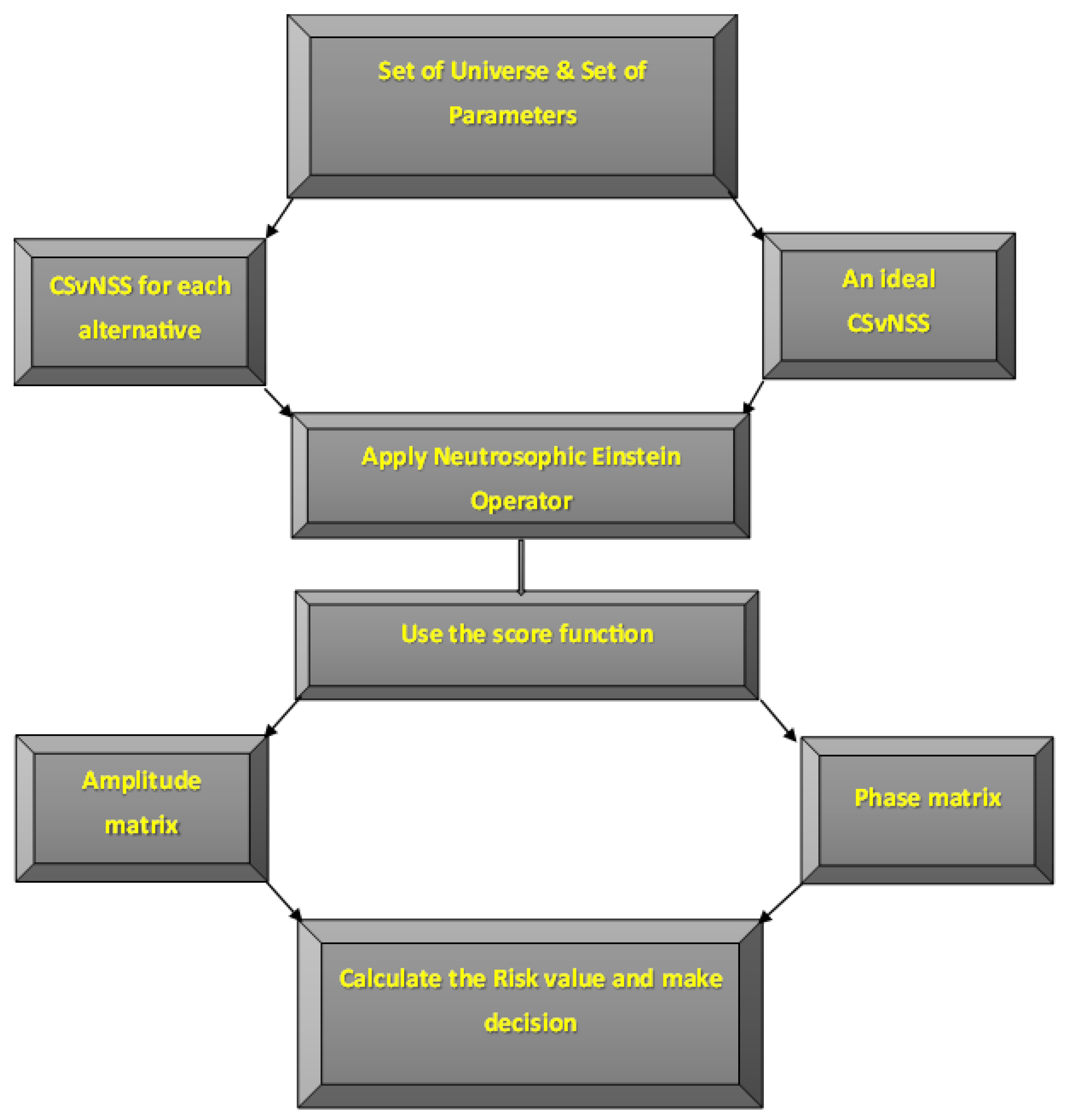
The proposed multi-attribute decision-making (MADM) framework is designed to support risk assessment under uncertain, indeterminate, and complex-valued decision information. The framework integrates the complex single-valued neutrosophic soft set (CSvNSS) representation with the proposed Einstein aggregation operators and a risk-oriented decision mechanism. In the considered problem, each alternative is evaluated with respect to multiple risk parameters, while each assessment preserves truth, indeterminacy, falsity, amplitude, and phase information. Let $\mathcal{A}=\{A_1,A_2,\dots ,A_m\}$, denote the set of alternatives and $\mathcal{C}=\{C_1,C_2,\dots ,C_n\}$ denote the set of decision criteria. Each assessment is represented using a complex single-valued neutrosophic number of the form $\tilde{\eta }=⟨t{e}^{i2\pi \tau },\iota e^{i2\pi \mu },f{e}^{i2\pi \varphi }⟩,$ where $t,\iota ,f\in [0,1]$ are the truth, indeterminacy, and falsity amplitudes, respectively, while $\tau ,\mu ,\varphi \in [0,1]$ denote their corresponding normalized phase components. The overall decision process consists of the following stages.

• Using the available information and the assessments provided by the experts, construct the complex single-valued neutrosophic soft decision matrices

  $${\aleph }_1,{\aleph }_2,\dots ,{\aleph }_K,$$

  where K denotes the number of experts. Each matrix represents the assessment of the alternatives with respect to the selected parameters. A general entry of the rth decision matrix is expressed as

  $${\aleph }_p({⋎}_j,{⋏}_d)=\left({\mathsf{F}}_{m+}^r\left({⋏}_d\right),{\mathsf{F}}_m^r\left({⋏}_d\right),{\mathsf{F}}_{m-}^r\left({⋏}_d\right)\right),$$

  where ${\mathsf{F}}_{m+}^r={\mathfrak{b}}_{m+}^r{e}^{\iota 2\pi {\mathfrak{c}}_{m+}^r}$, ${\mathsf{F}}_m^r={\mathfrak{b}}_m^r{e}^{\iota 2\pi {\mathfrak{c}}_m^r},$ and ${\mathsf{F}}_{m-}^r={\mathfrak{b}}_{m-}^r{e}^{\iota 2\pi {\mathfrak{c}}_{m-}^r}.$
• Construct an ideal complex single-valued neutrosophic soft decision matrix ${\aleph }^{\ast }$, with the assistance of domain experts. The ideal matrix represents the reference assessment against which the alternatives are evaluated. For each parameter–alternative pair, the corresponding ideal assessment is denoted by

  $${\aleph }^{\ast }({⋎}_j,{⋏}_d)=\left({\mathsf{F}}_{m+}^{\ast },{\mathsf{F}}_m^{\ast },{\mathsf{F}}_{m-}^{\ast }\right).$$
• For each alternative ${⋏}_d$, combine its corresponding CSvNSS assessment with the ideal assessment by using the introduced neutrosophic Einstein sum. Thus,

  $${\mathsf{F}}_d={\aleph }^{\ast }{\oplus }_{nes}{\aleph }_d,i=1,2,\dots ,m.$$
  The resulting matrix ${\mathsf{F}}_d$ contains the aggregated complex truth, indeterminacy, and falsity information associated with the ith alternative.
• For each complex single-valued neutrosophic number

  $${\mathsf{F}}_d({⋎}_j,{⋏}_d)=\left({\mathsf{F}}_{m+},{\mathsf{F}}_m,{\mathsf{F}}_{m-}\right),$$

  calculate its score value by using the score function defined as

  $$\mathcal{S}\left({\mathsf{F}}_{m+},{\mathsf{F}}_m,{\mathsf{F}}_{m-}\right)=\left({\mathfrak{b}}_{m+}+{\mathfrak{b}}_m-{\mathfrak{b}}_{m-}\right)e^{\iota 2\pi \left({\mathfrak{c}}_{m+}+{\mathfrak{c}}_m-{\mathfrak{c}}_{m-}\right)}.$$
  Since ${\mathfrak{b}}_{m+},{\mathfrak{b}}_m,{\mathfrak{b}}_{m-}\in [0,1],$ it follows that $-1\le \left({\mathfrak{b}}_{m+}+{\mathfrak{b}}_m{\mathfrak{b}}_{m-}\right)\le 2.$ Thus, the score function simultaneously incorporates the amplitude and phase information of the truth, indeterminacy, and falsity components. The score values obtained from all entries of ${\mathsf{F}}_d$ are subsequently used to construct the corresponding amplitude and phase matrices.
• Decompose the complex-valued score matrix into its amplitude and phase components. For the ith alternative, let

  $${\mathsf{F}}_{Ai}={\left[{\zeta }_{pq}^{\left(i\right)}\right]}_{m\times n}=\left(\begin{array}{cccc}{\zeta }_{11}^{\left(i\right)}& {\zeta }_{12}^{\left(i\right)}& \cdots & {\zeta }_{1n}^{\left(i\right)}\\ {\zeta }_{21}^{\left(i\right)}& {\zeta }_{22}^{\left(i\right)}& \cdots & {\zeta }_{2n}^{\left(i\right)}\\ ⋮& ⋮& \ddots & ⋮\\ {\zeta }_{m1}^{\left(i\right)}& {\zeta }_{m2}^{\left(i\right)}& \cdots & {\zeta }_{mn}^{\left(i\right)}\end{array}\right)$$

  denote the amplitude matrix, and let

  $${\mathsf{F}}_{Pi}={\left[{\varsigma }_{pq}^{\left(i\right)}\right]}_{m\times n}=\left(\begin{array}{cccc}{\varsigma }_{11}^{\left(i\right)}& {\varsigma }_{12}^{\left(i\right)}& \cdots & {\varsigma }_{1n}^{\left(i\right)}\\ {\varsigma }_{21}^{\left(i\right)}& {\varsigma }_{22}^{\left(i\right)}& \cdots & {\varsigma }_{2n}^{\left(i\right)}\\ ⋮& ⋮& \ddots & ⋮\\ {\varsigma }_{m1}^{\left(i\right)}& {\varsigma }_{m2}^{\left(i\right)}& \cdots & {\varsigma }_{mn}^{\left(i\right)}\end{array}\right)$$

  denote the corresponding phase matrix.
• Calculate the normalized risk value of the ith alternative according to

  $${\mathfrak{R}}_d={\displaystyle \frac{1}{2mn}}{\displaystyle \sum _{p=1}^m}{\displaystyle \sum _{q=1}^n}\left[{\left(1-{\zeta }_{pq}^{\left(i\right)}\right)}^2+{\left({\zeta }_{pq}^{\left(i\right)}\right)}^2+{\left(1-{\varsigma }_{pq}^{\left(i\right)}\right)}^2+{\left({\varsigma }_{pq}^{\left(i\right)}\right)}^2\right].$$
  The first two terms quantify the deviation of the amplitude component from its two limiting reference states, while the remaining two terms measure the corresponding deviation in the phase domain. The factor $2mn$ scales the accumulated amplitude and phase contributions according to the dimensions of the decision matrix, thereby facilitating consistent comparison among alternatives.
  Mathematical properties and interpretation of the risk function.
  To clarify the mathematical behavior of the proposed risk measure, define

  $$h\left(x\right)={(1-x)}^2+x^2=2{\left(x-{\displaystyle \frac{1}{2}}\right)}^2+{\displaystyle \frac{1}{2}}.$$
  Accordingly, the proposed risk function can be expressed as

  $$R_d={\displaystyle \frac{1}{2mn}}{\displaystyle \sum _{p=1}^m}{\displaystyle \sum _{q=1}^n}\left[h\left({\zeta }_{pq}^{\left(i\right)}\right)+h\left({\varsigma }_{pq}^{\left(i\right)}\right)\right].$$
  The following mathematical properties follow directly from this representation.
  • $h\left(x\right)$ is continuous and nonnegative.
  • $h\left(x\right)$ is strictly convex and attains its unique minimum at $x=1/2$, which follows from

    $$h^{\prime }\left(x\right)=4x-2,h^{″}\left(x\right)=4>0.$$
    Thus, score components located closer to the central reference level contribute less to the overall risk value, whereas components farther from this level make a larger contribution.
  • The function $h\left(x\right)$ is symmetric with respect to the two limiting reference states 0 and 1, that is, $h\left(x\right)=h(1-x)$.
    Consequently, the terms ${(1-{\zeta }_{pq}^{\left(i\right)})}^2+{\left({\zeta }_{pq}^{\left(i\right)}\right)}^2$ measure the joint deviation of the amplitude component from these two limiting states, while ${(1-{\varsigma }_{pq}^{\left(i\right)})}^2+{\left({\varsigma }_{pq}^{\left(i\right)}\right)}^2$ perform the same role for the corresponding phase component.
  • The proposed risk measure is separable across the entries of the decision matrix. Hence, each parameter–state combination contributes explicitly to the total risk, and no single matrix entry can determine the final ranking independently. The factor $1/\left(2mn\right)$ scales the accumulated contribution according to the size of the decision matrix, thereby allowing risk values obtained for different alternatives within the same decision environment to be compared consistently.
  The resulting value $R_d$ should therefore be interpreted as an aggregate measure of the deviation contained in the amplitude and phase information of the ith alternative. A smaller value of $R_d$ indicates a comparatively lower aggregate risk contribution, whereas a larger value indicates a stronger overall deviation in the score-derived amplitude and phase information. Accordingly, the decision rule selects the alternative associated with the minimum risk value.
• Rank all alternatives according to their risk values:

  $${\mathfrak{R}}_{d_1}\le {\mathfrak{R}}_{d_2}\le \cdots \le {\mathfrak{R}}_{d_m}.$$
  The alternative corresponding to the minimum risk value is selected as the most desirable alternative:

  $${\mathfrak{R}}_{d^{\ast }}=mi{n}_{1\le i\le m}{\mathfrak{R}}_d.$$
  Hence, ${⋏}_{d^{\ast }}$ is considered the optimal alternative under the proposed Einstein operator-based MADM framework.

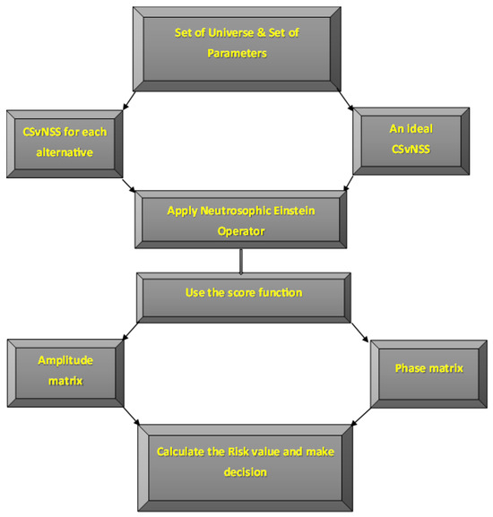
The proposed architecture shown in Figure 1 also preserves the multidimensional information contained in the CSvNSS representation throughout the aggregation process. In particular, the truth, indeterminacy, falsity, amplitude, and phase components are not reduced to a single real-valued representation before aggregation. This feature is consistent with the motivation of the proposed framework, in which complex-valued information is intended to preserve information that may be lost under conventional real-valued decision representations.

Figure 1. Architecture of proposed framework.

4.1. Computational Complexity Analysis

The computational complexity of the proposed framework is analyzed in terms of the number of alternatives, decision criteria, experts, and scalar components contained in each CSvNSS assessment. Let m denote the number of alternatives, n the number of decision criteria, and K the number of experts. To avoid ambiguity with the matrix indices used in the preceding formulation, the number of scalar components processed in each CSvNSS assessment is denoted by d. In the present CSvNSS representation, each assessment contains six scalar components, namely three amplitude components and three normalized phase components; hence, $d=6$.

The construction of the decision information requires processing each alternative–criterion–expert combination. Therefore, the computational cost of constructing and organizing the CSvNSS decision information is $O\left(mnKd\right).$ Since $d=6$ is fixed for the present CSvNSS representation, this term reduces to $O\left(mnK\right).$ The proposed Einstein aggregation operators process the components of the CSvNSS assessments using a constant number of elementary operations for each component. Consequently, for fixed d, the aggregation of the weighted decision information requires $O\left(mn\right)$. The subsequent score and risk calculations are performed for each alternative. Their computational costs are $O\left(md\right)$ for score evaluation and $O\left(md\right)$ for risk evaluation, respectively.

Finally, ranking m alternatives according to their risk values requires $O\left(m\log m\right)$ time when a standard comparison-based sorting procedure is used. The principal computational stages are summarized in Table 1.

Table 1. Computational complexity of the proposed MADM framework.

Stage	Main Operation	Complexity
1	CSvNSS decision-information construction	$O\left(mnKd\right)$
2	Einstein aggregation and weighting	$O\left(mnd\right)$
3	Score computation	$O\left(md\right)$
4	Risk evaluation	$O\left(md\right)$
5	Alternative ranking	$O\left(m\log m\right)$

For the proposed CSvNSS representation, $d=6$ is constant. Therefore, the overall computational complexity can be expressed as $O(mnK+m\log m).$ When the number of experts is also fixed, the complexity becomes $O(mn+m\log m).$ Thus, the dominant computational cost of the framework is associated with the construction and aggregation of the alternative-criterion information, whereas the final score, risk, and ranking operations have lower asymptotic complexity. The analysis indicates that the proposed methodology remains computationally tractable as the numbers of alternatives and criteria increase, although the computational cost naturally grows with the number of experts and the overall size of the decision environment.

4.2. Sensitivity and Robustness Analysis

Sensitivity analysis is conducted to examine the robustness of the obtained decision with respect to changes in the principal components of the proposed MADM framework. In particular, three sources of variation are considered: criterion weights, the selected Einstein aggregation operator, and the underlying CSvNSS assessment information. The purpose of this analysis is not to claim universal superiority of the proposed method, but to determine whether the preferred alternative remains stable under controlled perturbations.

Criterion-Weight Sensitivity

Let $\omega =({\omega }_1,{\omega }_2,\dots ,{\omega }_n)$, denote the normalized criterion-weight vector satisfying ${\omega }_j\ge 0,{\sum }_{j=1}^n{\omega }_j=1.$ To evaluate the influence of an individual criterion, the original weight ${\omega }_j$ is perturbed by a relative amount $\delta$, where $\delta \in \{-0.30,-0.20,-0.10,0.10,0.20,0.30\}.$ The perturbed weight is initially defined as ${\omega }_j^{\prime }={\omega }_j(1+\delta ).$

The remaining weights are subsequently renormalized according to

$${\omega }_k^{\prime }={\displaystyle \frac{{\omega }_k}{{\displaystyle {\displaystyle \sum _{\ell =1}^n}{\omega }_{\ell }^{\prime }}}},k=1,\dots ,n,$$

such that ${\sum }_{k=1}^n{\omega }_k^{\prime }=1.$ For every perturbed weight vector, the complete decision procedure is repeated and the resulting risk values and alternative ranking are recorded. This procedure identifies whether moderate changes in the importance assigned to an individual risk criterion can change the preferred alternative.

For the business-location problem, the four criteria are Market Competition (MC), Supply Chain issues (SCi), Production Scalability (PS), and Autonomous Driving Challenges (ADC), as shown in Table 2. These are the four principal risk parameters defined in the case study.

Table 2. Criterion-weight sensitivity analysis protocol.

Parameter	Perturbation	Procedure
MC	$\delta =\pm 0.10,\pm 0.20,\pm 0.30$	Perturb and renormalize weights
SCi	$\delta =\pm 0.10,\pm 0.20,\pm 0.30$	Perturb and renormalize weights
PS	$\delta =\pm 0.10,\pm 0.20,\pm 0.30$	Perturb and renormalize weights
ADC	$\delta =\pm 0.10,\pm 0.20,\pm 0.30$	Perturb and renormalize weights

The principal robustness indicator is the stability of the selected alternative. If the preferred alternative remains unchanged over the considered perturbation range, the decision can be regarded as stable with respect to the corresponding criterion-weight variation.

4.3. Case Study: Business Location Selection

To demonstrate the applicability of the proposed Einstein operator-based CSvNSS MADM framework, a business location selection problem is considered. The purpose of this case study is to identify the most appropriate location for establishing a handicraft business while minimizing the associated risk. The case study is used as an illustrative decision environment in which uncertainty and, when available, temporal or seasonal risk information can be represented simultaneously. The example is not intended to imply that every business-location problem necessarily requires complex-valued information.

Consider a decision maker, denoted by Richard, who intends to establish an international handicraft business in the United States. Three potential locations are under consideration: Portland, Austin, and Los Angeles, denoted, respectively, by ${\mathfrak{A}}_1,{\mathfrak{A}}_2,{\mathfrak{A}}_3.$ The proposed business focuses on unique, high-quality, and sustainable handmade products, including wooden crafts, textile and embroidery products, handmade jewelry and accessories, and handmade bags. Since the long-term objective is to develop an internationally scalable business, the selection of an appropriate location must account for both immediate operational conditions and potential future risks.

For illustrative purposes, four location-related risk criteria are considered: ${⋏}_1$: Market Competition (MC), ${⋏}_2:$ Supply Chain issues (SCi), ${⋏}_3$: Production Scalability (PS), ${⋏}_4$: Skilled Artisan Availability and Retention (SAAR). These criteria represent four distinct dimensions of the proposed handicraft business. Market competition reflects the intensity of the local and regional competitive environment; supply-chain issues represent uncertainty in sourcing materials and delivering products; production scalability captures the ability to expand output as demand increases; and skilled artisan availability and retention represents the risk associated with recruiting and retaining workers possessing the specialized manual and craft skills required for handmade production.

4.3.1. Interpretation and Elicitation of the Phase Components

In the present application, the phase components are interpreted as temporal-location variables within a normalized annual business-risk cycle. Let one complete business cycle correspond to a one-year reference horizon. A normalized phase value $\theta \in [0,1),$ therefore represents a temporal position within this cycle, and the corresponding complex phase angle is $2\pi \theta$.

For a CSvNSN $\mathfrak{n}=⟨t{e}^{i2\pi \tau },\iota e^{i2\pi \mu },f{e}^{i2\pi \varphi }⟩,$ the amplitude components t, $\iota$, and f quantify, respectively, the strengths of the truth, indeterminacy, and falsity assessments associated with a specified risk state. Their corresponding phase components have a temporal interpretation. Specifically, $\tau$ indicates the position within the annual cycle at which the evidence supporting the considered risk state is strongest, $\mu$ indicates the position at which uncertainty regarding that risk state is greatest, and $\varphi$ indicates the position at which the evidence opposing that risk state is strongest.

For example, a normalized phase value close to $0.25$ represents a peak around the end of the first quarter of the annual cycle, whereas values close to $0.50$ and $0.75$ represent approximately mid-year and the third-quarter period, respectively. Consequently, two alternatives may have similar risk amplitudes but different phase components when the same degree of risk is expected to occur at different times of the business cycle.

In a practical application, the amplitude and phase information should be elicited separately. Experts are first asked to assess the strength of truth, indeterminacy, and falsity associated with each risk state. They are subsequently asked to identify the period within the adopted business cycle during which each of these assessments is expected to be most pronounced. If month h, $h=1,\dots ,12$, is identified as the relevant peak period, the corresponding normalized phase can be encoded as $\theta ={\displaystyle \frac{h-1}{12}}.$ Quarterly, seasonal, or other application-specific cycles may be used instead, provided that the reference period is defined before the elicitation process and applied consistently to all alternatives.

Within the present business-location setting, such temporal information may be relevant when market competition varies with seasonal demand, supply-chain disruption varies across procurement or transportation periods, or production scalability changes across high- and low-demand periods. Hence, the phase component is intended to supplement the magnitude of a risk assessment with information concerning its timing within a recurring decision horizon.

It should be emphasized that the use of a complex-valued neutrosophic representation is not necessary for every business-risk problem. If the available assessments contain only magnitude information and no meaningful cyclic, seasonal, or phase-dependent component can be identified, a real-valued neutrosophic model provides a more parsimonious representation. The additional complex phase component becomes useful when the timing of otherwise similar risk assessments is itself decision-relevant. Therefore, the present case study should be viewed primarily as an illustration of the computational capability of the proposed CSvNSS framework under phase-augmented information rather than as evidence that all business-location problems inherently require a complex representation.

Because the numerical assessments used in the present case study are hypothetical, the reported phase values should be interpreted as synthetic temporal assessments constructed to demonstrate the phase-aware computational procedure. in an empirical implementation, these values would be obtained using the elicitation protocol described above.

4.3.2. Construction of the Ideal CSvNSS Decision Matrix

The ideal CSvNSS decision matrix serves as a common reference profile against which the candidate alternatives are evaluated. To make the construction procedure reproducible, the ideal matrix is obtained through a structured expert-elicitation process.

Let $E_k$, $k=1,2,\dots ,K$ denote the participating domain experts, and let $C_j$, $j=1,2,\dots ,n$ denote the decision criteria. For each risk state r and criterion $C_j$, expert $E_k$ specifies an ideal complex single-valued neutrosophic assessment of the form

$${\mathfrak{n}}_{pj}^{\ast \left(k\right)}=⟨t_{pj}^{\ast \left(k\right)}{e}^{i2\pi {\tau }_{pj}^{\ast \left(k\right)}},{\iota }_{pj}^{\ast \left(k\right)}{e}^{i2\pi {\mu }_{pj}^{\ast \left(k\right)}},f_{pj}^{\ast \left(k\right)}{e}^{i2\pi {\phi }_{pj}^{\ast \left(k\right)}}⟩,$$

where

$$t_{pj}^{\ast \left(k\right)},{\iota }_{pj}^{\ast \left(k\right)},f_{pj}^{\ast \left(k\right)},{\tau }_{pj}^{\ast \left(k\right)},{\mu }_{pj}^{\ast \left(k\right)},{\phi }_{pj}^{\ast \left(k\right)}\in [0,1].$$

Here, $t_{pj}^{\ast \left(k\right)}$, ${\iota }_{pj}^{\ast \left(k\right)}$, and $f_{pj}^{\ast \left(k\right)}$ represent the truth, indeterminacy, and falsity amplitudes assigned by the kth expert, whereas ${\tau }_{pj}^{\ast \left(k\right)}$, ${\mu }_{pj}^{\ast \left(k\right)}$, and ${\phi }_{pj}^{\ast \left(k\right)}$ represent the corresponding normalized phase components. The experts determine these values according to their assessment of the reference condition associated with the considered risk state and criterion.

When more than one expert participates, the individual ideal assessments are combined to obtain a consensus reference assessment. Let $\mathsf{\lambda }=({\lambda }_1,{\lambda }_2,\dots ,{\lambda }_K)$, be the expert-weight vector, where ${\lambda }_k\ge 0,{\sum }_{k=1}^K{\lambda }_k=1.$ The aggregated ideal assessment for the rth risk state and the jth criterion is then obtained as

$${\mathfrak{n}}_{pj}^{\ast }={\mathrm{NEWAAO}}_{\mathsf{\lambda }}\left({\mathfrak{n}}_{pj}^{\ast \left(1\right)},{\mathfrak{n}}_{pj}^{\ast \left(2\right)},\dots ,{\mathfrak{n}}_{pj}^{\ast \left(K\right)}\right).$$

If all experts are considered equally important, then ${\lambda }_k=1/K$. Finally, arranging the aggregated ideal assessments for all risk states and criteria gives the ideal CSvNSS decision matrix ${\aleph }^{\ast }=\left[{\mathfrak{n}}_{pj}^{\ast }\right].$

This matrix is common to all candidate alternatives and provides the reference information used in the subsequent Einstein aggregation and risk-evaluation stages. The same construction procedure can therefore be applied to another case study by redefining the alternatives, criteria, risk states, and corresponding expert reference assessments.

4.3.3. Decision Information for Portland

The CSvNSS decision matrix associated with Portland ${\mathfrak{A}}_1$ is constructed from the expert assessments given in ${\aleph }_{{\mathfrak{A}}_1}$. The rows correspond to the three risk states, whereas the columns represent the four risk parameters. The resulting matrix is denoted by ${\aleph }_{{\mathfrak{A}}_1}$ and is given by

$${\aleph }_{{\mathfrak{A}}_1}=\left(\begin{array}{cccc}⟨\begin{array}{c}{0.47}^{i2\pi 0.14}\\ {0.64}^{i2\pi 0.23}\\ {0.63}^{i2\pi 0.31}\end{array}⟩& ⟨\begin{array}{c}{0.70}^{i2\pi 0.18}\\ {0.56}^{i2\pi 0.27}\\ {0.72}^{i2\pi 0.36}\end{array}⟩& ⟨\begin{array}{c}{0.64}^{i2\pi 0.24}\\ {0.68}^{i2\pi 0.33}\\ {0.50}^{i2\pi 0.42}\end{array}⟩& ⟨\begin{array}{c}{0.62}^{i2\pi 0.29}\\ {0.89}^{i2\pi 0.46}\\ {0.64}^{i2\pi 0.54}\end{array}⟩\\ ⟨\begin{array}{c}{0.48}^{i2\pi 0.14}\\ {0.63}^{i2\pi 0.23}\\ {0.67}^{i2\pi 0.31}\end{array}⟩& ⟨\begin{array}{c}{0.72}^{i2\pi 0.18}\\ {0.58}^{i2\pi 0.27}\\ {0.73}^{i2\pi 0.35}\end{array}⟩& ⟨\begin{array}{c}{0.85}^{i2\pi 0.25}\\ {0.59}^{i2\pi 0.30}\\ {0.51}^{i2\pi 0.37}\end{array}⟩& ⟨\begin{array}{c}{0.59}^{i2\pi 0.28}\\ {0.67}^{i2\pi 0.42}\\ {0.55}^{i2\pi 0.57}\end{array}⟩\\ ⟨\begin{array}{c}{0.61}^{i2\pi 0.22}\\ {0.59}^{i2\pi 0.38}\\ {0.47}^{i2\pi 0.45}\end{array}⟩& ⟨\begin{array}{c}{0.73}^{i2\pi 0.29}\\ {0.67}^{i2\pi 0.35}\\ {0.52}^{i2\pi 0.41}\end{array}⟩& ⟨\begin{array}{c}{0.63}^{i2\pi 0.24}\\ {0.56}^{i2\pi 0.34}\\ {0.51}^{i2\pi 0.42}\end{array}⟩& ⟨\begin{array}{c}{0.71}^{i2\pi 0.28}\\ {0.68}^{i2\pi 0.45}\\ {0.65}^{i2\pi 0.53}\end{array}⟩\end{array}\right).$$

Construct the ideal complex single-valued neutrosophic soft decision matrix ${\aleph }^{\ast }$ according to the expert-elicitation and aggregation procedure described above. The ideal matrix provides a common reference profile for all candidate alternatives.

$${\aleph }^{\ast }=\left(\begin{array}{cccc}⟨\begin{array}{c}{0.84}^{i2\pi 0.15}\\ {0.86}^{i2\pi 0.24}\\ {0.92}^{i2\pi 0.32}\end{array}⟩& ⟨\begin{array}{c}{0.87}^{i2\pi 0.19}\\ {0.78}^{i2\pi 0.28}\\ {0.85}^{i2\pi 0.37}\end{array}⟩& ⟨\begin{array}{c}{0.96}^{i2\pi 0.26}\\ {0.83}^{i2\pi 0.34}\\ {0.74}^{i2\pi 0.43}\end{array}⟩& ⟨\begin{array}{c}{0.85}^{i2\pi 0.30}\\ {0.91}^{i2\pi 0.48}\\ {0.78}^{i2\pi 0.55}\end{array}⟩\\ ⟨\begin{array}{c}{0.49}^{i2\pi 0.16}\\ {0.77}^{i2\pi 0.25}\\ {0.89}^{i2\pi 0.33}\end{array}⟩& ⟨\begin{array}{c}{0.95}^{i2\pi 0.20}\\ {0.82}^{i2\pi 0.29}\\ {0.78}^{i2\pi 0.38}\end{array}⟩& ⟨\begin{array}{c}{0.89}^{i2\pi 0.27}\\ {0.81}^{i2\pi 0.31}\\ {0.75}^{i2\pi 0.39}\end{array}⟩& ⟨\begin{array}{c}{0.98}^{i2\pi 0.29}\\ {0.80}^{i2\pi 0.44}\\ {0.78}^{i2\pi 0.58}\end{array}⟩\\ ⟨\begin{array}{c}{0.83}^{i2\pi 0.23}\\ {0.81}^{i2\pi 0.39}\\ {0.79}^{i2\pi 0.46}\end{array}⟩& ⟨\begin{array}{c}{0.94}^{i2\pi 0.30}\\ {0.79}^{i2\pi 0.36}\\ {0.85}^{i2\pi 0.42}\end{array}⟩& ⟨\begin{array}{c}{0.91}^{i2\pi 0.25}\\ {0.78}^{i2\pi 0.35}\\ {0.82}^{i2\pi 0.43}\end{array}⟩& ⟨\begin{array}{c}{0.82}^{i2\pi 0.29}\\ {0.90}^{i2\pi 0.47}\\ {0.86}^{i2\pi 0.54}\end{array}⟩\end{array}\right).$$

4.3.4. Aggregation Using the Neutrosophic Einstein Sum

The ideal matrix is subsequently combined with the decision matrix of Portland using the proposed neutrosophic Einstein sum. According to the defined Einstein sum, we obtain ${\mathsf{F}}_1={\aleph }_{{\mathfrak{A}}_1}{\oplus }_{nes}{\aleph }^{\ast }.$ The resulting aggregated CSvNSS matrix is

$${\mathsf{F}}_1=\left(\begin{array}{cccc}⟨\begin{array}{c}{0.94}^{i2\pi 0.28}\\ {0.97}^{i2\pi 0.34}\\ {0.99}^{i2\pi 0.45}\end{array}⟩& ⟨\begin{array}{c}{0.97}^{i2\pi 0.35}\\ {0.92}^{i2\pi 0.42}\\ {0.88}^{i2\pi 0.28}\end{array}⟩& ⟨\begin{array}{c}{0.99}^{i2\pi 0.42}\\ {0.95}^{i2\pi 0.36}\\ {0.84}^{i2\pi 0.51}\end{array}⟩& ⟨\begin{array}{c}{0.99}^{i2\pi 0.54}\\ {0.89}^{i2\pi 0.22}\\ {0.87}^{i2\pi 0.33}\end{array}⟩\\ ⟨\begin{array}{c}{0.78}^{i2\pi 0.29}\\ {0.96}^{i2\pi 0.36}\\ {0.99}^{i2\pi 0.41}\end{array}⟩& ⟨\begin{array}{c}{0.98}^{i2\pi 0.34}\\ {0.93}^{i2\pi 0.39}\\ {0.92}^{i2\pi 0.26}\end{array}⟩& ⟨\begin{array}{c}{0.99}^{i2\pi 0.41}\\ {0.89}^{i2\pi 0.37}\\ {0.82}^{i2\pi 0.49}\end{array}⟩& ⟨\begin{array}{c}{0.98}^{i2\pi 0.52}\\ {0.90}^{i2\pi 0.24}\\ {0.85}^{i2\pi 0.35}\end{array}⟩\\ ⟨\begin{array}{c}{0.95}^{i2\pi 0.29}\\ {0.91}^{i2\pi 0.33}\\ {0.89}^{i2\pi 0.46}\end{array}⟩& ⟨\begin{array}{c}{0.99}^{i2\pi 0.36}\\ {0.89}^{i2\pi 0.41}\\ {0.91}^{i2\pi 0.29}\end{array}⟩& ⟨\begin{array}{c}{0.97}^{i2\pi 0.42}\\ {0.98}^{i2\pi 0.38}\\ {0.72}^{i2\pi 0.51}\end{array}⟩& ⟨\begin{array}{c}{0.97}^{i2\pi 0.49}\\ {0.97}^{i2\pi 0.26}\\ {0.96}^{i2\pi 0.22}\end{array}⟩\end{array}\right).$$

Applying the proposed score function to each element of ${\mathsf{F}}_1$ yields the following complex-valued score matrix:

$${\mathsf{F}}_1^S=\left(\begin{array}{cccc}{0.96}^{i2\pi 0.39}& {0.93}^{i2\pi 0.31}& {0.88}^{i2\pi 0.57}& {0.97}^{i2\pi 0.64}\\ {0.81}^{i2\pi 0.34}& {0.97}^{i2\pi 0.21}& {0.92}^{i2\pi 0.54}& {0.93}^{i2\pi 0.63}\\ {0.94}^{i2\pi 0.42}& {1.01}^{i2\pi 0.24}& {0.71}^{i2\pi 0.55}& {0.96}^{i2\pi 0.45}\end{array}\right).$$

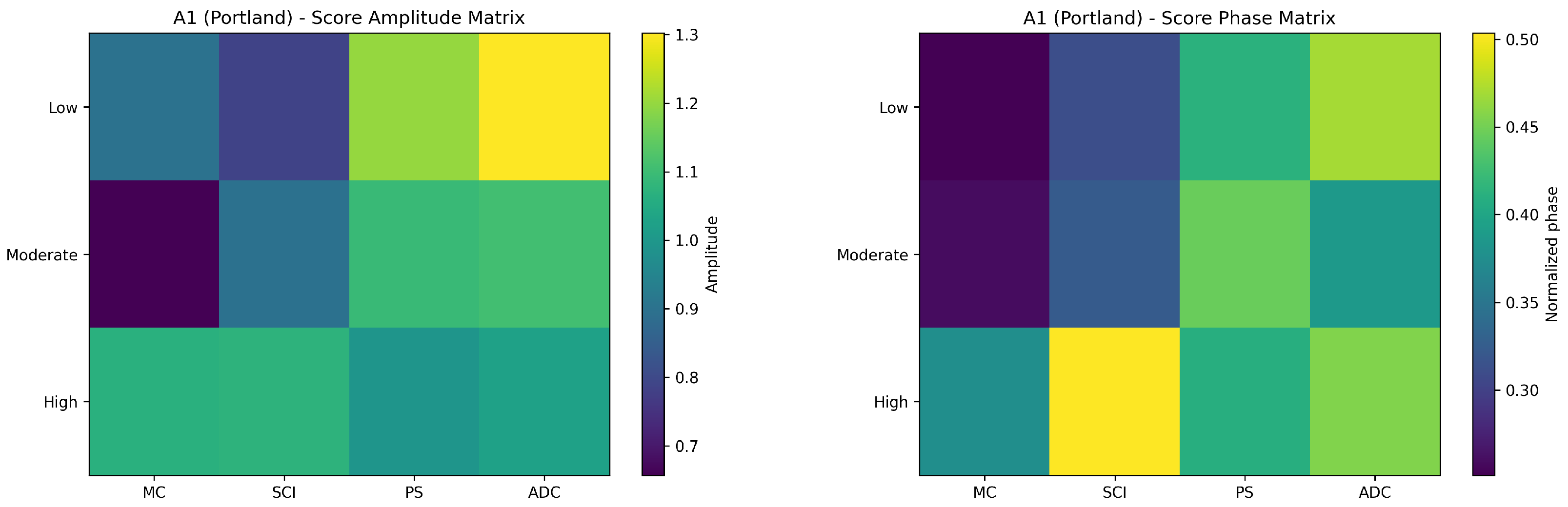
The corresponding amplitude and phase matrices are therefore

$${\mathsf{F}}_{1A}=\left(\begin{array}{cccc}0.96& 0.93& 0.88& 0.97\\ 0.81& 0.97& 0.92& 0.93\\ 0.94& 1.01& 0.71& 0.96\end{array}\right),$$

and

$${\mathsf{F}}_{1P}=2\pi \left(\begin{array}{cccc}0.39& 0.31& 0.57& 0.64\\ 0.34& 0.21& 0.54& 0.63\\ 0.42& 0.24& 0.55& 0.45\end{array}\right).$$

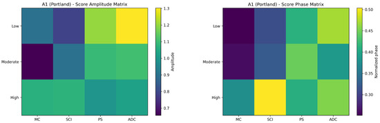
The amplitude and phase components of the complex score matrix for ${\mathfrak{A}}_1$ are visualized in Figure 2. Substitution of these amplitude and phase values into the proposed risk function gives ${\mathfrak{R}}_1=1.5857.$

Figure 2. Amplitude and phase component of the score matrix for ${\mathfrak{A}}_1$.

4.3.5. Assessment of Austin and Los Angeles

Following the same computational procedure, the CSvNSS decision matrices for Austin ${\mathfrak{A}}_2$ and Los Angeles ${\mathfrak{A}}_3$ are given by

$${\aleph }_{{\mathfrak{A}}_2}=\left(\begin{array}{cccc}⟨\begin{array}{c}{0.50}^{i2\pi 0.15}\\ {0.69}^{i2\pi 0.24}\\ {0.68}^{i2\pi 0.32}\end{array}⟩& ⟨\begin{array}{c}{0.67}^{i2\pi 0.19}\\ {0.66}^{i2\pi 0.28}\\ {0.65}^{i2\pi 0.37}\end{array}⟩& ⟨\begin{array}{c}{0.76}^{i2\pi 0.26}\\ {0.73}^{i2\pi 0.34}\\ {0.54}^{i2\pi 0.43}\end{array}⟩& ⟨\begin{array}{c}{0.85}^{i2\pi 0.30}\\ {0.71}^{i2\pi 0.48}\\ {0.68}^{i2\pi 0.55}\end{array}⟩\\ ⟨\begin{array}{c}{0.59}^{i2\pi 0.16}\\ {0.70}^{i2\pi 0.25}\\ {0.71}^{i2\pi 0.33}\end{array}⟩& ⟨\begin{array}{c}{0.55}^{i2\pi 0.20}\\ {0.62}^{i2\pi 0.29}\\ {0.78}^{i2\pi 0.38}\end{array}⟩& ⟨\begin{array}{c}{0.69}^{i2\pi 0.27}\\ {0.57}^{i2\pi 0.31}\\ {0.53}^{i2\pi 0.39}\end{array}⟩& ⟨\begin{array}{c}{0.58}^{i2\pi 0.29}\\ {0.68}^{i2\pi 0.44}\\ {0.58}^{i2\pi 0.58}\end{array}⟩\\ ⟨\begin{array}{c}{0.63}^{i2\pi 0.23}\\ {0.61}^{i2\pi 0.39}\\ {0.49}^{i2\pi 0.46}\end{array}⟩& ⟨\begin{array}{c}{0.74}^{i2\pi 0.30}\\ {0.69}^{i2\pi 0.36}\\ {0.55}^{i2\pi 0.42}\end{array}⟩& ⟨\begin{array}{c}{0.61}^{i2\pi 0.25}\\ {0.78}^{i2\pi 0.35}\\ {0.52}^{i2\pi 0.43}\end{array}⟩& ⟨\begin{array}{c}{0.72}^{i2\pi 0.29}\\ {0.90}^{i2\pi 0.47}\\ {0.66}^{i2\pi 0.54}\end{array}⟩\end{array}\right),$$

and

$${\aleph }_{{\mathfrak{A}}_3}=\left(\begin{array}{cccc}⟨\begin{array}{c}{0.52}^{i2\pi 0.17}\\ {0.71}^{i2\pi 0.26}\\ {0.66}^{i2\pi 0.35}\end{array}⟩& ⟨\begin{array}{c}{0.65}^{i2\pi 0.21}\\ {0.68}^{i2\pi 0.30}\\ {0.63}^{i2\pi 0.39}\end{array}⟩& ⟨\begin{array}{c}{0.78}^{i2\pi 0.28}\\ {0.75}^{i2\pi 0.37}\\ {0.56}^{i2\pi 0.46}\end{array}⟩& ⟨\begin{array}{c}{0.83}^{i2\pi 0.32}\\ {0.73}^{i2\pi 0.50}\\ {0.70}^{i2\pi 0.57}\end{array}⟩\\ ⟨\begin{array}{c}{0.61}^{i2\pi 0.18}\\ {0.72}^{i2\pi 0.27}\\ {0.73}^{i2\pi 0.36}\end{array}⟩& ⟨\begin{array}{c}{0.57}^{i2\pi 0.22}\\ {0.64}^{i2\pi 0.31}\\ {0.80}^{i2\pi 0.40}\end{array}⟩& ⟨\begin{array}{c}{0.71}^{i2\pi 0.29}\\ {0.59}^{i2\pi 0.33}\\ {0.55}^{i2\pi 0.41}\end{array}⟩& ⟨\begin{array}{c}{0.60}^{i2\pi 0.31}\\ {0.70}^{i2\pi 0.46}\\ {0.60}^{i2\pi 0.60}\end{array}⟩\\ ⟨\begin{array}{c}{0.65}^{i2\pi 0.25}\\ {0.63}^{i2\pi 0.41}\\ {0.51}^{i2\pi 0.48}\end{array}⟩& ⟨\begin{array}{c}{0.76}^{i2\pi 0.32}\\ {0.71}^{i2\pi 0.38}\\ {0.57}^{i2\pi 0.44}\end{array}⟩& ⟨\begin{array}{c}{0.63}^{i2\pi 0.27}\\ {0.80}^{i2\pi 0.37}\\ {0.54}^{i2\pi 0.45}\end{array}⟩& ⟨\begin{array}{c}{0.74}^{i2\pi 0.31}\\ {0.92}^{i2\pi 0.49}\\ {0.68}^{i2\pi 0.56}\end{array}⟩\end{array}\right).$$

Applying Steps 4–7 of the proposed procedure to these two decision matrices produces the corresponding risk values ${\mathfrak{R}}_2=1.8135,{\mathfrak{R}}_3=1.4691.$

4.3.6. Decision Analysis

The resulting risk values for the three candidate locations are ${\mathfrak{R}}_1=1.5857,{\mathfrak{R}}_2=1.8135,{\mathfrak{R}}_3=1.4691.$ Consequently, the alternatives are ranked according to ${\mathfrak{R}}_3<{\mathfrak{R}}_1<{\mathfrak{R}}_2.$ Because the proposed decision criterion selects the alternative associated with the minimum risk value, Los Angeles, ${\mathfrak{A}}_3$ is identified as the preferred location for the proposed handicraft business.

It is worth emphasizing that the decision is obtained after integrating the complete complex neutrosophic information rather than by considering a single risk parameter independently. The resulting ranking therefore reflects the joint contribution of the four risk parameters and their corresponding truth, indeterminacy, falsity, amplitude, and phase information.

4.4. Aggregation Operator-Based Sensitivity

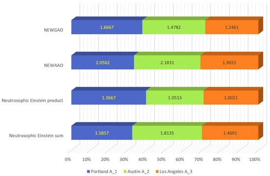
The sensitivity of the proposed decision procedure to the choice of Einstein aggregation mechanism is examined by applying four aggregation operators to the same synthetic business-location decision information. Specifically, the neutrosophic Einstein sum ${\oplus }_{nes}$, neutrosophic Einstein product ${\otimes }_{nep}$, NEWAAO, and NEWGAO are considered. The purpose of this experiment is to characterize how the selected aggregation rule influences the computed risk indices and resulting rankings. Because the underlying decision information is hypothetical, the analysis is interpreted as an internal behavioral comparison rather than empirical validation or evidence of superior decision accuracy.

The resulting risk values and alternative rankings are reported in Table 3.

Table 3. Risk values and rankings obtained using different Einstein-based aggregation operators.

Operator	${\mathfrak{A}}_1$	${\mathfrak{A}}_2$	${\mathfrak{A}}_3$	Ranking
${\oplus }_{nes}$	1.5857	1.8135	1.4691	${\mathfrak{A}}_3<{\mathfrak{A}}_1<{\mathfrak{A}}_2$
${\otimes }_{nep}$	1.3667	1.0513	1.0021	${\mathfrak{A}}_3<{\mathfrak{A}}_2<{\mathfrak{A}}_1$
NEWAAO	2.0562	2.1831	1.9021	${\mathfrak{A}}_3<{\mathfrak{A}}_1<{\mathfrak{A}}_2$
NEWGAO	1.6667	1.4782	1.2461	${\mathfrak{A}}_3<{\mathfrak{A}}_2<{\mathfrak{A}}_1$

Several observations can be drawn from Table 3. The four aggregation mechanisms identify $A_3$ as the first-ranked alternative for the considered synthetic decision matrix. However, the ordering of $A_1$ and $A_2$ differs between the sum-type and product-type operators. Thus, the experiment shows that the identity of the first-ranked alternative is stable across the four tested aggregation mechanisms, whereas the ordering of the remaining alternatives is sensitive to the aggregation rule.

First, all four Einstein-based aggregation mechanisms identify ${\mathfrak{A}}_3$ as the first-ranked alternative for the considered synthetic decision matrix. This agreement indicates that the identity of the first-ranked alternative is insensitive to the tested aggregation operator within this numerical experiment. It should not, however, be interpreted as evidence that ${\mathfrak{A}}_3$ is the objectively correct alternative or that one aggregation mechanism is more accurate than another, because no external ground-truth ranking is available for the hypothetical data. Second, the relative ordering of the remaining alternatives varies across aggregation operators. These differences illustrate the behavioral sensitivity of the MADM procedure to the selected aggregation rule and show how different nonlinear operators process the same CSvNSS information. Accordingly, the operator comparison is used to characterize ranking behavior and internal stability, rather than to measure predictive or decision accuracy.

Most importantly, the stability of the first-ranked alternative across all four operators indicates that the selection of ${\mathfrak{A}}_3$ is not an artifact of a single aggregation rule. Rather, the available decision information provides consistent support for ${\mathfrak{A}}_3$ as the lowest-risk location.

The graphical representation of the risk values obtained from the different Einstein operators is presented in Figure 3.

Figure 3. Risk values obtained using different Einstein-based aggregation operators.

4.4.1. Input-Information Sensitivity

A second sensitivity experiment considers perturbations in the underlying CSvNSS assessment information. Each CSvNSS assessment contains truth, indeterminacy, and falsity amplitudes together with their corresponding phase components. Let

$$ϵ\in \{-0.05,-0.02,0.02,0.05\}$$

denote a perturbation magnitude.

For an amplitude component x, the perturbed value is defined as

$$x^{\prime }=\min \left(1,\max (0,x+ϵ)\right).$$

The same bounded perturbation principle can be applied to the normalized phase components. The complete MADM procedure is then repeated using the perturbed CSvNSS information (see Table 4).

Table 4. Input-information sensitivity analysis protocol.

Component	Perturbation	Constraint
Truth amplitude	$ϵ=\pm 0.02,\pm 0.05$	$[0,1]$
indeterminacy amplitude	$ϵ=\pm 0.02,\pm 0.05$	$[0,1]$
Falsity amplitude	$ϵ=\pm 0.02,\pm 0.05$	$[0,1]$
Truth phase	$ϵ=\pm 0.02,\pm 0.05$	$[0,1]$
indeterminacy phase	$ϵ=\pm 0.02,\pm 0.05$	$[0,1]$
Falsity phase	$ϵ=\pm 0.02,\pm 0.05$	$[0,1]$

The objective of this experiment is to determine whether small changes in expert assessments can alter the final decision. The resulting risk values are compared with the baseline values and the corresponding ranking is recorded.

This analysis is particularly relevant because the proposed CSvNSS representation explicitly preserves both amplitude and phase information. Consequently, robustness should be examined not only with respect to criterion weights but also with respect to the information encoded within the complex neutrosophic assessments.

4.4.2. Robustness Indicators

Three indicators are proposed to summarize the sensitivity experiments. First, the ranking stability rate is defined as

$$\mathrm{RSR}={\displaystyle \frac{N_{\mathrm{stable}}}{N_{\mathrm{total}}}}\times 100\%,$$

where $N_{\mathrm{stable}}$ is the number of perturbation scenarios for which the preferred alternative remains unchanged and $N_{\mathrm{total}}$ is the total number of tested scenarios. Second, the normalized risk deviation for alternative $A_d$ is defined as

$${\mathrm{NRD}}_d={\displaystyle \frac{|R_d^{\prime }-R_d|}{\max (R_d,{\epsilon }_0)}},$$

where $R_d$ is the baseline risk value, $R_d^{\prime }$ is the perturbed risk value, and ${\epsilon }_0>0$ is a small numerical constant used to avoid division by zero. Third, the rank-change count is defined as

$${\mathrm{RCC}}_d={\displaystyle \sum _{s=1}^N}\beth \left({\mathrm{rank}}_{d,s}^{\prime }\ne {\mathrm{rank}}_{d,s}\right),$$

where N is the number of sensitivity scenarios and $\beth (·)$ is the indicator function.

The complete sensitivity-analysis protocol is summarized in Table 5.

Table 5. Overall sensitivity and robustness analysis protocol.

Analysis	Tested Factor	Main Robustness Indicator
Weight sensitivity	Criterion weights	Ranking stability
Operator sensitivity	Einstein aggregation operator	Preferred-alternative stability
input sensitivity	CSvNSS amplitudes and phases	Ranking stability
Risk deviation	Perturbed versus baseline risk	Normalized risk deviation
Rank sensitivity	Alternative positions	Rank-change count

4.5. Case Study and Reproducibility of the Sensitivity Analysis

The business-location case study provides the numerical environment for evaluating the proposed methodology. Three candidate locations are considered: Portland ($A_1$), Austin ($A_2$), and Los Angeles ($A_3$). Four principal risk parameters are used, namely Market Competition (MC), Supply Chain issues (SCi), Production Scalability (PS), and Autonomous Driving Challenges (ADC). Three linguistic risk states are considered: Low Risk, Moderate Risk, and High Risk. The original computational analysis reports the risk values

$$R_1=1.5857,R_2=1.8135,R_3=1.4691,$$

which gives the ranking $A_3<A_1<A_2.$ Because the decision rule selects the alternative with the minimum risk value, $A_3$, corresponding to Los Angeles, is selected as the preferred location. The original analysis emphasizes that this decision is obtained by integrating the complete complex neutrosophic information rather than relying on a single risk parameter. For reproducibility, every sensitivity experiment should preserve the same alternative set, criterion set, CSvNSS representation, ideal decision information, aggregation definitions, score function, and risk function used in the baseline experiment. Only the parameter under investigation should be modified. The reproducibility requirements are summarized in Table 6.

Table 6. Reproducibility requirements for the proposed sensitivity analysis.

Item	Requirement
Alternatives	$A_1$, $A_2$, and $A_3$
Risk parameters	MC, SCi, PS, and ADC
information structure	CSvNSS
Primary operator	${\oplus }_{nes}$
Alternative operators	${\otimes }_{nep}$, NEWAAO, and NEWGAO
Baseline ranking	$A_3<A_1<A_2$
Decision rule	Minimum risk value is preferred
Weight experiment	Perturb, normalize, and repeat the full procedure
input experiment	Perturb bounded CSvNSS components and repeat the procedure
Output	Risk values, rankings, RSR, NRD, and RCC

The sensitivity analysis should be interpreted as a robustness assessment for the considered numerical decision environment. It does not constitute empirical validation because the data used in the case study are hypothetical and were generated for demonstrating the proposed methodology. Accordingly, the sensitivity experiments provide computational evidence regarding internal stability rather than evidence of performance on an external real-world dataset. The combination of operator sensitivity, criterion-weight sensitivity, and input-information sensitivity provides a more comprehensive assessment of the proposed framework. In particular, operator sensitivity evaluates the influence of the aggregation mechanism, weight sensitivity evaluates the influence of decision preferences, and input-information sensitivity evaluates the influence of uncertainty in the underlying CSvNSS assessments. Together, these analyses provide a systematic basis for discussing the robustness and limitations of the proposed MADM methodology.

4.6. Additional Numerical Validation Examples

To examine the scalability of the proposed framework beyond the original three-alternative illustration, two controlled synthetic decision problems are considered. The same four risk criteria are retained: Market Competition (MC), Supply Chain issues (SCi), Production Scalability (PS), and Autonomous Driving Challenges (ADC). The three risk states are also retained as Low, Moderate, and High. In both experiments, the same ideal CSvNSS reference matrix used in the main case study is employed, and the same Einstein aggregation, score, risk, and ranking procedures are applied. For compact presentation, define $[t,\iota ,f\mid \tau ,\mu ,\phi ]\equiv ⟨t{e}^{i2\pi \tau },\iota e^{i2\pi \mu },f{e}^{i2\pi \phi }⟩.$

4.6.1. Five-Alternative Validation Example

The baseline CSvNSS profile is

$${\mathcal{B}}^{\left(5\right)}=\left(\begin{array}{cccc}[0.48,0.68,0.65\mid 0.15,0.24,0.31]& [0.53,0.72,0.68\mid 0.19,0.28,0.36]& [0.58,0.76,0.71\mid 0.23,0.32,0.41]& [0.63,0.80,0.74\mid 0.27,0.36,0.46]\\ [0.54,0.65,0.60\mid 0.19,0.29,0.36]& [0.59,0.69,0.63\mid 0.23,0.33,0.41]& [0.64,0.73,0.66\mid 0.27,0.37,0.46]& [0.69,0.77,0.69\mid 0.31,0.41,0.51]\\ [0.60,0.62,0.55\mid 0.23,0.34,0.41]& [0.65,0.66,0.58\mid 0.27,0.38,0.46]& [0.70,0.70,0.61\mid 0.31,0.42,0.51]& [0.75,0.74,0.64\mid 0.35,0.46,0.56]\end{array}\right)$$

For a perturbation parameter $\delta$, each baseline entry $[t,\iota ,f\mid \tau ,\mu ,\phi ]$ is transformed according to

$$[t+\delta ,\iota -0.50\delta ,f-0.70\delta \mid \tau +0.40\delta ,\mu -0.30\delta ,\phi -0.40\delta ].$$

The five alternatives are generated using ${\delta }_{B_1}=0,{\delta }_{B_2}=0.08,{\delta }_{B_3}=-0.04,{\delta }_{B_4}=0.04,{\delta }_{B_5}=-0.08,$ all generated components remain inside $[0,1]$ as shown in Table 7. Applying the complete proposed procedure gives

$$R_{B_1}=0.7961,R_{B_2}=0.8118,R_{B_3}=0.7891,R_{B_4}=0.8037,R_{B_5}=0.7827.$$

Therefore, $B_5\prec B_3\prec B_1\prec B_4\prec B_2,$ and $B_5$ is selected as the minimum-risk alternative.

Table 7. Risk results for the five-alternative validation example.

Alternative	Perturbation $\mathsf{\delta }$	Risk Value
$B_1$	$0.00$	$0.7961$
$B_2$	$0.08$	$0.8118$
$B_3$	$-0.04$	$0.7891$
$B_4$	$0.04$	$0.8037$
$B_5$	$-0.08$	$0.7827$

4.6.2. Seven-Alternative Validation Example

A second, independent baseline profile is defined as

$${\mathcal{B}}^{\left(7\right)}=\left(\begin{array}{cccc}[0.52,0.63,0.60\mid 0.18,0.28,0.35]& [0.55,0.68,0.64\mid 0.23,0.31,0.39]& [0.58,0.73,0.68\mid 0.28,0.34,0.43]& [0.61,0.78,0.72\mid 0.33,0.37,0.47]\\ [0.57,0.65,0.57\mid 0.21,0.32,0.39]& [0.60,0.70,0.61\mid 0.26,0.35,0.43]& [0.63,0.75,0.65\mid 0.31,0.38,0.47]& [0.66,0.80,0.69\mid 0.36,0.41,0.51]\\ [0.62,0.67,0.54\mid 0.24,0.36,0.43]& [0.65,0.72,0.58\mid 0.29,0.39,0.47]& [0.68,0.77,0.62\mid 0.34,0.42,0.51]& [0.71,0.82,0.66\mid 0.39,0.45,0.55]\end{array}\right)$$

For this experiment, each baseline entry is transformed as $[t+0.80\delta ,\iota +0.40\delta ,f-0.60\delta \mid \tau -0.30\delta ,\mu +0.50\delta ,\phi -0.40\delta ].$ The seven alternatives are generated using

$${\delta }_{C_1}=0.03,{\delta }_{C_2}=-0.09,{\delta }_{C_3}=0.09,{\delta }_{C_4}=-0.03,{\delta }_{C_5}=0.06,{\delta }_{C_6}=0,{\delta }_{C_7}=-0.06.$$

Again, all generated components remain inside $[0,1]$, as shown in Table 8. The resulting risk values are $R_{C_1}=0.8528,R_{C_2}=0.7350,R_{C_3}=0.9210,R_{C_4}=0.7907,R_{C_5}=0.8861,R_{C_6}=0.8210,R_{C_7}=0.7621.$ Hence, $C_2\prec C_7\prec C_4\prec C_6\prec C_1\prec C_5\prec C_3,$ and $C_2$ is identified as the minimum-risk alternative.

Table 8. Risk results for the seven-alternative validation example.

Alternative	Perturbation $\mathsf{\delta }$	Risk Value
$C_1$	$0.03$	$0.8528$
$C_2$	$-0.09$	$0.7350$
$C_3$	$0.09$	$0.9210$
$C_4$	$-0.03$	$0.7907$
$C_5$	$0.06$	$0.8861$
$C_6$	$0.00$	$0.8210$
$C_7$	$-0.06$	$0.7621$

These two experiments demonstrate that the mathematical structure of the proposed CSvNSS–Einstein MADM procedure does not depend on a fixed number of alternatives. The same reference matrix, aggregation rule, score function, and risk function can be applied without modification as the alternative set is expanded. Because the additional data are synthetic, these experiments should be interpreted as numerical scalability and internal-consistency validation rather than empirical validation using an external real-world dataset.

5. Comparative Analysis

To broaden the validation of the proposed CSvNSS–Einstein framework, its ranking results were compared with three classical MADM methods: Simple Additive Weighting (SAW), TOPSiS, and the RAnking based on Distance And Range (RADAR) method. Since these methods require a real-valued decision matrix, the original CSvNSS assessments were first transformed into crisp criterion-level scores. This transformation is used only for benchmarking and does not replace the complex-valued representation employed by the proposed method. For an input CSvNSN

$${\mathfrak{n}}_{drj}=⟨t_{drj}{e}^{i2\pi {\tau }_{drj}},{\iota }_{drj}{e}^{i2\pi {\mu }_{drj}},f_{drj}{e}^{i2\pi {\phi }_{drj}}⟩,$$

where i denotes the alternative, r the risk state, and j the criterion, the amplitude and normalized-phase score components are defined, consistently with the score structure used in the proposed framework, as

$$a_{drj}=t_{drj}+{\iota }_{drj}-f_{drj},p_{drj}={\tau }_{drj}+{\mu }_{drj}-{\phi }_{drj}.$$

Because $a_{drj},p_{drj}\in [-1,2]$, they are linearly mapped to the unit interval and combined with equal importance:

$$d_{drj}={\displaystyle \frac{1}{2}}\left({\displaystyle \frac{a_{drj}+1}{3}}+{\displaystyle \frac{p_{drj}+1}{3}}\right)={\displaystyle \frac{a_{drj}+p_{drj}+2}{6}}.$$

The three linguistic risk-state assessments are then averaged to obtain the crisp alternative–criterion value $x_{dj}={\displaystyle \frac{1}{3}}{\sum }_{p=1}^3{d}_{drj}.$ Applying this transformation to the input matrices of Portland ($A_1$), Austin ($A_2$), and Los Angeles ($A_3$) gives

$$X=\left(\begin{array}{cccc}0.4400& 0.4672& 0.4956& 0.4922\\ 0.4528& 0.4667& 0.5044& 0.5067\\ 0.4606& 0.4733& 0.5111& 0.5111\end{array}\right),$$

where the columns correspond, respectively, to Market Competition (MC), Supply Chain issues (SCi), Production Scalability (PS), and Autonomous Driving Challenges (ADC). Since the resulting entries are preference scores, all four columns are treated as benefit-type criteria in the classical MADM benchmark. To isolate the effect of the ranking method itself, equal criterion weights are used $\mathbf{w}=(0.25,0.25,0.25,0.25).$

5.1. Benchmark Comparison

5.1.1. SAW Benchmark

For SAW [34,35], the crisp matrix is normalized according to $N_{dj}={\displaystyle \frac{x_{dj}}{{\max }_d{x}_{dj}}},$ and the overall score of alternative $A_d$ is $Q_d^{\mathrm{SAW}}={\sum }_{j=1}^4{w}_j{N}_{dj}.$ The resulting scores are $Q_1^{\mathrm{SAW}}=0.9688,Q_2^{\mathrm{SAW}}=0.9868,Q_3^{\mathrm{SAW}}=1.0000.$ Thus, SAW gives $A_3\succ A_2\succ A_1.$

5.1.2. TOPSiS Benchmark

For TOPSiS [36], vector normalization is first applied $r_{dj}={\displaystyle \frac{x_{dj}}{\sqrt{{\sum }_{d=1}^3{x}_{dj}^2}}},v_{dj}=w_j{r}_{dj}.$ Because all criteria are benefit-type, the positive and negative ideal solutions are $v_j^{+}={\max }_d{v}_{dj},v_j^{-}={\min }_d{v}_{dj}.$ The Euclidean distances from the two ideal solutions are

$$D_d^{+}=\sqrt{\sum _{j=1}^4{(v_{dj}-v_j^{+})}^2},D_d^{-}=\sqrt{\sum _{j=1}^4{(v_{dj}-v_j^{-})}^2},$$

and the relative closeness coefficient is $C_d={\displaystyle \frac{D_d^{-}}{D_d^{+}+D_d^{-}}}.$ The obtained values are $C_1=0.0171,C_2=0.6161,C_3=1.0000,$ which yields $A_3\succ A_2\succ A_1.$

5.1.3. RADAR Benchmark

The RADAR method [37,38,39] is also applied to the same crisp matrix and weight vector. For a benefit-type criterion, the maximum- and minimum-proportion coefficients are calculated as

$${\alpha }_{dj}={\displaystyle \frac{{\max }_d{x}_{dj}/x_{dj}}{\left({\max }_d{x}_{dj}/x_{dj}\right)+\left(x_{dj}/{\min }_d{x}_{dj}\right)}},\mathrm{and}{\beta }_{dj}={\displaystyle \frac{x_{dj}/{\min }_d{x}_{dj}}{\left({\max }_d{x}_{dj}/x_{dj}\right)+\left(x_{dj}/{\min }_d{x}_{dj}\right)}}.$$

The empty range and relative relationship are $E_{dj}=|{\alpha }_{dj}-{\beta }_{dj}|,R{R}_{dj}={\displaystyle \frac{{\alpha }_{dj}}{{\beta }_{dj}+E_{dj}}},$ followed by $WR{R}_{dj}=w_{j}R{R}_{dj}.$ Let $S_d={\sum }_{j=1}^{4}WR{R}_{dj}$; the RADAR ranking index is $R{i}_d={\displaystyle \frac{{\min }_{\ell }{S}_{\ell }}{S_d}},$ where a larger value indicates a better-ranked alternative. The resulting indices are $R{i}_1=0.9391,R{i}_2=0.9561,R{i}_3=1.0000.$ Accordingly, RADAR also produces $A_3\succ A_2\succ A_1.$

The comparison in Table 9 shows that all four approaches identify $A_3$ (Los Angeles) as the preferred alternative. Thus, the principal decision is preserved after reducing the complex neutrosophic information to a crisp representation and applying three methodologically different MADM procedures. However, the relative positions of $A_1$ and $A_2$ differ. The proposed CSvNSS–Einstein framework ranks $A_1$ ahead of $A_2$, whereas SAW, TOPSiS, and RADAR rank $A_2$ ahead of $A_1$. This difference is expected because the crisp benchmarking procedure compresses the truth, indeterminacy, falsity, amplitude, and phase information before ranking, while the proposed framework retains the complete CSvNSS structure throughout the Einstein aggregation and risk-evaluation stages. Therefore, the classical comparison does not indicate universal superiority of one method over another. Rather, it shows that the selection of the first-ranked alternative is robust across substantially different MADM principles, while the ordering of the non-optimal alternatives remains sensitive to the information representation and aggregation mechanism.

Table 9. Comparison of the proposed CSvNSS–Einstein framework with classical MADM approaches.

Method	${\mathit{A}}_1$	${\mathit{A}}_2$	${\mathit{A}}_3$	Ranking
Proposed CSvNSS–Einstein $R_d$ (smaller is better)	1.5857	1.8135	1.4691	$A_3\succ A_1\succ A_2$
SAW $Q_d$ (larger is better)	0.9688	0.9868	1.0000	$A_3\succ A_2\succ A_1$
TOPSiS $C_d$ (larger is better)	0.0171	0.6161	1.0000	$A_3\succ A_2\succ A_1$
RADAR $R{i}_d$ (larger is better)	0.9391	0.9561	1.0000	$A_3\succ A_2\succ A_1$

To further assess the proposed CSvNSS framework and its associated MADM methodology, the comparison is conducted from two complementary perspectives. First, a structural comparison is performed to highlight the representational capabilities of CSvNSS relative to existing fuzzy, intuitionistic, picture fuzzy, and neutrosophic soft set frameworks. Second, a computational comparison is conducted by applying representative existing MADM approaches to the same business-location selection problem.

5.2. Structural Comparative Analysis

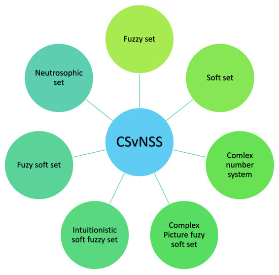
The proposed CSvNSS framework is compared with the complex fuzzy soft set [25], complex intuitionistic fuzzy soft set [26], complex picture fuzzy soft set [27], and single-valued neutrosophic soft set [40].

The principal distinction of CSvNSS lies in its simultaneous treatment of parameterization, three independent neutrosophic components, and complex-valued information. In particular, the framework explicitly represents truth, indeterminacy, and falsity through complex-valued quantities. Consequently, each component possesses both an amplitude and a phase representation. This construction provides two complementary modeling capabilities. The soft-set component facilitates parameter-dependent representation of the decision environment, while the neutrosophic component allows truth, indeterminacy, and falsity to be modeled independently. The complex extension further enables the representation of phase information that cannot be captured by conventional real-valued membership structures.

Accordingly, the proposed CSvNSS framework offers a more expressive representation for decision environments in which uncertainty, indeterminacy, parameter dependence, and phase-related information occur simultaneously. The structural relationship among the considered frameworks is illustrated in Figure 4.

Figure 4. Structural comparison of the proposed CSvNSS framework with selected existing soft-set-based structures.

5.3. Computational Comparative Analysis

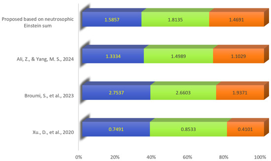
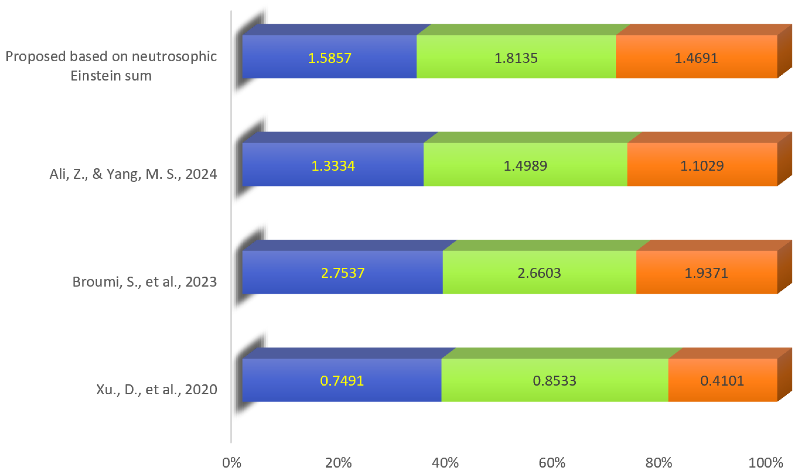
The computational performance of the proposed MADM methodology is further examined by comparing its results with representative decision-making approaches reported by Xu et al. [41], Broumi et al. [42], and Ali and Yang [43]. To ensure a meaningful comparison, the corresponding methods are applied to the same business-location case study and evaluated using the same set of alternatives and decision parameters.

The comparative results are illustrated in Figure 5. The analysis shows that the considered approaches identify ${\mathfrak{A}}_3$ as the preferred alternative. The agreement among the methods provides evidence that the proposed framework produces a decision that is consistent with alternative MADM formulations.

Figure 5. Comparative risk values obtained from the proposed and selected existing [41,42,43] MADM approaches.

However, the primary contribution of the proposed approach is not merely the identification of the same optimal alternative. Its principal advantage lies in the richer representation of the underlying decision information. Existing approaches may aggregate the available assessments through conventional real-valued or reduced-dimensional representations, whereas the proposed CSvNSS framework preserves truth, indeterminacy, falsity, amplitude, and phase information throughout the decision process.

Therefore, the comparative analysis suggests that the proposed framework can provide a more informative representation of uncertain decision environments while retaining a clear and computationally tractable ranking mechanism. The agreement in the first-ranked alternative across the proposed and comparative methods indicates consistency of the ranking outcome for the considered synthetic decision environment. Since the underlying data are hypothetical and no externally validated reference ranking is available, this agreement does not establish decision accuracy, predictive validity, or the superiority of any method.

5.4. Discussion of the Comparative Findings

The numerical experiments provide three important observations. First, the proposed Einstein operator-based methodology successfully transforms complex neutrosophic soft information into an interpretable risk-based ranking. Second, the optimal alternative, ${\mathfrak{A}}_3$, remains unchanged when the principal Einstein aggregation mechanism is replaced by the other proposed Einstein operators. Third, the same alternative is obtained when the proposed method is compared with representative existing MADM approaches.

These findings indicate that the decision obtained for the present case study is relatively stable with respect to the choice of aggregation mechanism. Nevertheless, the differences in the risk magnitudes and in the ordering of the non-optimal alternatives demonstrate that the choice of aggregation operator can influence the degree of separation among alternatives. This observation is consistent with the nonlinear nature of Einstein aggregation and highlights the importance of selecting an operator according to the information structure and decision-maker requirements.

It should also be noted that agreement in the optimal alternative should not, by itself, be interpreted as proof of universal superiority. Rather, the present computational experiment demonstrates the applicability, consistency, and representational advantages of the proposed CSvNSS-based methodology for the considered decision problem. A broader assessment involving additional datasets, sensitivity analysis, expert groups, and diverse decision scenarios would provide stronger evidence regarding the generalization and robustness of the proposed framework.

6. Conclusions

This article introduces the hybrid structure of the complex single-valued neutrosophic soft set, along with an illustrative example to aid in understanding its fundamental definition. Subsequently, the definitions of the neutrosophic Einstein sum and the neutrosophic Einstein product are presented, each followed by an example. Furthermore, the neutrosophic Einstein weighted average aggregation operator (NEWAAO) and the neutrosophic Einstein weighted geometric aggregation operator (NEWGAO) are introduced as generalized forms of the neutrosophic Einstein sum and the neutrosophic Einstein product, respectively.

In the application section, the proposed MADM procedure is illustrated through a hypothetical business-location risk assessment problem. Together with the additional synthetic numerical examples, sensitivity analysis, and comparative experiments, the results demonstrate the computational feasibility, numerical consistency, and scalability of the proposed framework within the considered decision environments.

The present study does not establish empirical predictive performance or real-world decision reliability, since the numerical assessments are hypothetical and no external dataset is used. Consequently, the framework should presently be regarded as a methodological and computational decision-support model. Future work should evaluate the approach using real expert assessments, observed business-risk data, independent datasets, and decision problems from other application domains before broader claims regarding generalizability or practical effectiveness can be made.

Limitations and Scope of Validation

The numerical analyses presented in this study should be interpreted within the scope of methodological and computational validation rather than empirical validation. The primary business-location example is based on hypothetical CSvNSS assessments and does not employ an external observational dataset. Accordingly, the obtained rankings demonstrate the operation of the proposed Einstein aggregation and risk-evaluation framework under a controlled decision environment, but they do not establish its predictive accuracy or decision reliability for actual business-location problems.

To examine whether the proposed procedure depends on a fixed number of alternatives, additional five- and seven-alternative synthetic decision problems were also considered. These experiments provide evidence of numerical scalability and internal consistency; however, because the additional assessments are also synthetic, they should not be regarded as independent empirical validation.

Similarly, the sensitivity analyses evaluate the stability of the computed rankings under controlled changes in aggregation operators, criterion weights, and CSvNSS information. Such robustness reflects internal computational stability only and does not establish generalizability to unobserved real-world cases.

Therefore, the present results should be viewed as a proof-of-concept evaluation of the proposed CSvNSS–Einstein MADM framework. Empirical assessment would require real expert elicitation or observed business risk data, multiple decision environments, independent datasets, and comparison of the resulting recommendations with externally verified outcomes. Such validation constitutes an important direction for future research.

References

- Avramova, T.; Peneva, T.; Ivanov, A. Overview of existing multi-criteria decision-making (MCDM) methods used in industrial environments. Technologies 2025, 13, 444. [Google Scholar] [CrossRef] [Scilit]
- Zavadskas, E.K.; Antucheviciene, J.; Chatterjee, P. Multiple-criteria decision-making (MCDM) techniques for business processes information management. Information 2018, 10, 4. [Google Scholar] [CrossRef] [Scilit]
- Alexe, C.M.; Nechita, R.M. A Theoretical Framework for Multi-Attribute Decision- Making Methods in the intelligent Leading and Allocation of Human Resources in Research and Development Projects. Sustainability 2025, 17, 7535. [Google Scholar] [CrossRef] [Scilit]
- Markulik, Š.; Šolc, M.; Blaško, P. Use of Risk Management to Support Business Sustainability in the Automotive industry. Sustainability 2024, 16, 4308. [Google Scholar] [CrossRef] [Scilit]
- Jemai, J.; Zarrad, A. Feature selection engineering for credit risk assessment in retail banking. Information 2023, 14, 200. [Google Scholar] [CrossRef] [Scilit]
- Kiratsoudis, S.; Tsiantos, V. Advanced integration of ES-MADM II in HRM: A balanced approach to appraisal and promotion decisions. Information 2024, 15, 767. [Google Scholar] [CrossRef] [Scilit]
- Ahuja, N.; Kaur, R. An integrated fuzzy MADM framework for analyzing risk mitigation strategies in Digitally Sustainable Supply Chain. OPSEARCH 2025, 62, 1–41. [Google Scholar] [CrossRef] [Scilit]
- Choudhary, H.; Orra, A.; Sahoo, K.; Thakur, M. Risk-adjusted deep reinforcement learning for portfolio optimization: A multi-reward approach. Int. J. Comput. Intell. Syst. 2025, 18, 126. [Google Scholar] [CrossRef] [Scilit]
- Singh, S.; Singh, K. Q-rung orthopair fuzzy equivalences and related similarity measures with applications to pattern recognition and MADM. Comput. Appl. Math. 2025, 44, 251. [Google Scholar] [CrossRef] [Scilit]
- Ali, J. Multi-criteria decision-making method based on an integrated model using T-spherical fuzzy Aczel-Alsina prioritized aggregation operators. Comput. Appl. Math. 2025, 44, 181. [Google Scholar] [CrossRef] [Scilit]
- Liu, J.; Zhou, T. Fuzzy MADM for optimal bridge rehabilitation in transportation infrastructure maintenance. Int. J. Constr. Manag. 2026, 1–24. [Google Scholar] [CrossRef] [Scilit]
- Zadeh, L.A. Fuzzy sets. Inf. Control 1965, 8, 338–353. [Google Scholar] [CrossRef] [Scilit]
- Zimmermann, H.J. Fuzzy Set Theory—And Its Applications; Springer Science & Business Media: Berlin, Germany, 2011. [Google Scholar]
- Zadeh, L.A. Fuzzy logic—A personal perspective. Fuzzy Sets Syst. 2015, 281, 4–20. [Google Scholar] [CrossRef] [Scilit]
- Atanassov, K.T. Intuitionistic fuzzy sets. In Proceedings of the Vii iTKR’s Session, Sofia, Deposited in Central Science Technical Library of Bulgarian Academy of Sciences, Sofia, Bulgaria, 20–23 June 1983. [Google Scholar]
- Cuong, B.C.; Kreinovich, V. Picture fuzzy sets—A new concept for computational intelligence problems. In 2013 Third World Congress on Information and Communication Technologies (WICT 2013); IEEE: Piscataway, NJ, USA, 2013; pp. 1–6. [Google Scholar]
- Cuong, B.C.; Kreinovich, V. Picture fuzzy sets. J. Comput. Sci. Cybern. 2014, 30, 409–420. [Google Scholar] [CrossRef] [Scilit]
- Smarandache, F. Neutrosophic set—A generalization of the intuitionistic fuzzy set. In 2006 IEEE International Conference on Granular Computing; IEEE: Piscataway, NJ, USA, 2006; pp. 38–42. [Google Scholar]
- Wang, H.; Smarandache, F.; Zhang, Y.-Q.; Sunderraman, R. Single Valued Neutrosophic Sets; Infinite Study: Gallup, NM, USA, 2010. [Google Scholar]
- Molodtsov, D. Soft Set Theory—First Results. Comput. Math. Appl. 1999, 37, 19–31. [Google Scholar] [CrossRef] [Scilit]
- Çağman, N.; Enginoğlu, S.; Citak, F. Fuzzy soft set theory and its applications. Iran. J. Fuzzy Syst. 2011, 8, 137–147. [Google Scholar] [CrossRef] [Scilit]
- Xu, Y.J.; Sun, Y.K.; Li, D.F. Intuitionistic fuzzy soft set. In 2010 2nd International Workshop on Intelligent Systems and Applications; IEEE: Piscataway, NJ, USA, 2010; pp. 1–4. [Google Scholar]
- Yang, Y.; Liang, C.; Ji, S.; Liu, T. Adjustable soft discernibility matrix based on picture fuzzy soft sets and its applications in decision making. J. Intell. Fuzzy Syst. 2015, 29, 1711–1722. [Google Scholar] [CrossRef] [Scilit]
- Maji, P.K. Neutrosophic soft set. Ann. Fuzzy Math. Inform. 2013, 5, 157–168. [Google Scholar]
- Thirunavukarasu, P.; Suresh, R.; Ashokkumar, V. Theory of complex fuzzy soft set and its applications. Int. J. Innov. Res. Sci. Technol. 2017, 3, 13–18. [Google Scholar]
- Kumar, T.; Bajaj, R.K. On complex intuitionistic fuzzy soft sets with distance measures and entropies. J. Math. 2014, 2014, 972198. [Google Scholar] [CrossRef] [Scilit]
- Asghar, A.; Khan, K.A.; Albahar, M.A.; Alammari, A. An optimized multi-attribute decision-making approach to construction supply chain management by using complex picture fuzzy soft set. PeerJ Comput. Sci. 2023, 9, e1540. [Google Scholar] [CrossRef] [Scilit] [PubMed]
- Khan, K.A.; Asghar, A.; Rahman, A.U.; Mabela, R.M. An algorithmic multiple attribute decision-making context to model uncertainty associated with hospital site selection problem using complex SV-neutrosophic soft information. Appl. Artif. Intell. 2024, 38, 2375110. [Google Scholar] [CrossRef] [Scilit]
- Rahman, K.; Abdullah, S.; Hussain, F. Some generalised Einstein hybrid aggregation operators and their application to group decision-making using Pythagorean fuzzy numbers. Fuzzy Inf. Eng. 2019, 11, 412–427. [Google Scholar] [CrossRef] [Scilit]
- Rani, P.; Mishra, A.R. Fermatean fuzzy Einstein aggregation operators-based MULTIMOORA method for electric vehicle charging station selection. Expert Syst. Appl. 2021, 182, 115267. [Google Scholar] [CrossRef] [Scilit]
- Tanoli, M.N.K.; Rafique, K.; Mahmood, Z.; Abdalla, N.S.E.; Popa, I.L.; Kumar, A. Einstein aggregation operators for multicriteria group decision making in uncertain environments using cubic picture fuzzy sets. Sci. Rep. 2025, 15, 36545. [Google Scholar] [CrossRef] [Scilit] [PubMed]
- Zaman, T.; Khan, A.; Movaheedi, Z. An innovative approach to decision-making through cubical fuzzy Einstein hybrid aggregation operators. J. Big Data 2025, 13, 3. [Google Scholar] [CrossRef] [Scilit]
- Zhao, X.; Wei, G. Some intuitionistic fuzzy Einstein hybrid aggregation operators and their application to multiple attribute decision making. Knowl.-Based Syst. 2013, 37, 472–479. [Google Scholar] [CrossRef] [Scilit]
- Taherdoost, H. Analysis of simple additive weighting method (SAW) as a multiattribute decision-making technique: A step-by-step guide. J. Manag. Sci. Eng. Res. 2023, 6, 21–24. [Google Scholar] [CrossRef] [Scilit]
- Darvazeh, S.S.; MansooriMooseloo, F.; Acero-López, A.E. SAW: Simple additive weighting for multi-attribute decision-making. In Encyclopedia of Multi-Attribute Decision Making (MADM); Morgan Kaufmann: Cambridge, MA, USA, 2026; pp. 683–700. [Google Scholar]
- Papathanasiou, J.; Ploskas, N. Topsis. In Multiple Criteria Decision Aid: Methods, Examples and Python Implementations; Springer International Publishing: Cham, Switzerland, 2018; pp. 1–30. [Google Scholar]
- Komatina, N.; Marinković, D.; Petrović, N. RADAR: Ranking based on distance and range for multi-attribute decision-making. In Encyclopedia of Multi-Attribute Decision Making (MADM); Morgan Kaufmann: Burlington, MA, USA, 2026; pp. 1217–1230. [Google Scholar]
- Komatina, N. A compromise-based MADM approach for prioritizing failures: Integrating the RADAR method within the FMEA framework. J. Syst. Manag. Ind. 2024, 8, 73–88. [Google Scholar] [CrossRef] [Scilit]
- Xie, D.; Pan, Y.; Zhao, Y.; Wang, X.; Huang, Z. Radar jamming decision-making: A review. IEEE Access 2025, 13, 166800–166818. [Google Scholar] [CrossRef] [Scilit]
- Khalil, A.M.; Cao, D.; Azzam, A.; Smarandache, F.; Alharbi, W.R. Combination of the single-valued neutrosophic fuzzy set and the soft set with applications in decision-making. Symmetry 2020, 12, 1361. [Google Scholar] [CrossRef] [Scilit]
- Xu, D.; Cui, X.; Xian, H. An extended EDAS method with a single-valued complex neutrosophic set and its application in green supplier selection. Mathematics 2020, 8, 282. [Google Scholar] [CrossRef] [Scilit]
- Broumi, S.; Mohanaselvi, S.; Witczak, T.; Talea, M.; Bakali, A.; Smarandache, F. Complex Fermatean neutrosophic graph and application to decision making. Decis. Mak. Appl. Manag. Eng. 2023, 6, 474–501. [Google Scholar] [CrossRef] [Scilit]
- Ali, Z.; Yang, M.S. Improving risk assessment model for cyber security using robust aggregation operators for bipolar complex fuzzy soft inference systems. Mathematics 2024, 12, 582. [Google Scholar] [CrossRef] [Scilit]
Disclaimer/Publisher’s Note: The statements, opinions and data contained in all publications are solely those of the individual author(s) and contributor(s) and not of MDPI and/or the editor(s). MDPI and/or the editor(s) disclaim responsibility for any injury to people or property resulting from any ideas, methods, instructions or products referred to in the content. |
© 2026 by the authors. Licensee MDPI, Basel, Switzerland. This article is an open access article distributed under the terms and conditions of the Creative Commons Attribution (CC BY) license.