Graph Based Feature Selection for Reduction of Dimensionality in Next-Generation RNA Sequencing Datasets

Abstract

Analysis of high-dimensional data, with more features ($p$) than observations ($N$) ($p>N$), places significant demand in cost and memory computational usage attributes. Feature selection can be used to reduce the dimensionality of the data. We used a graph-based approach, principal component analysis (PCA) and recursive feature elimination to select features for classification from RNAseq datasets from two lung cancer datasets. The selected features were discretized for association rule mining where support and lift were used to generate informative rules. Our results show that the graph-based feature selection improved the performance of sequential minimal optimization (SMO) and multilayer perceptron classifiers (MLP) in both datasets. In association rule mining, features selected using the graph-based approach outperformed the other two feature-selection techniques at a support of 0.5 and lift of 2. The non-redundant rules reflect the inherent relationships between features. Biological features are usually related to functions in living systems, a relationship that cannot be deduced by feature selection and classification alone. Therefore, the graph-based feature-selection approach combined with rule mining is a suitable way of selecting and finding associations between features in high-dimensional RNAseq data.

1. Introduction

Analysis of high-dimensional data, with more features ($p$) than observations ($N$) ($p>>N$), places significant demand in cost and memory computational usage attributes. Analysis of high-dimensional data requires both high computational costs and computer memory usage [1]. Dimensionality reduction techniques that minimize the features in the original data without losing any important information have been used to address this challenge [2]. This reduces storage space and computational time and removes redundant, noisy and irrelevant data while improving algorithm efficiency as well as accuracy [3]. Feature selection and extraction constitute common approaches used to reduce dimensionality with the former identifying subsets of sufficient informative features that define the data. Major feature-selection techniques include filters, wrappers and embedded/hybrid techniques [4]. Wrappers follow a greedy search approach that wraps the feature selection around a learning algorithm and subsequently uses the accuracy of performance or error rate of the classification process as a criterion of feature evaluation. However, this approach is slower for a large feature space because every feature must be evaluated using a trained classifier. The filter method checks the features relying on the intrinsic characteristics (information, dependency, consistency and distance) prior to the learning tasks [5], which requires lower computational resources. Filters are thus faster but inefficient in classification relative to wrapper methods. Hybrid/embedded techniques are a combination of filters and wrappers [6]. We refer readers to the following articles and references therein for detailed reviews of feature-selection methods [7,8,9,10,11,12,13].

Feature-extraction techniques obtain the most important features from a dataset [14]. Principal component analysis (PCA), for example, uses covariance to extract relevant features from high-dimensional data [15]. A major drawback of feature-extraction techniques is their inaccuracy when mapping from a high-dimensional space to a low-dimensional space, which leads to the loss of data interpretability [16]. Another approach used in the analysis of big data is machine learning which has been defined as the ability of machines to learn without being programmed [17]. Classification is a supervised machine learning approach where labels are provided with the input data. Trained classifiers have been used in areas such as diabetes studies [18], cancer studies [19] and medical diagnosis [14]. Metrics such as accuracy, sensitivity, specificity, recall, robustness, computational scalability and computational cost are then used to evaluate the performance of the classifiers [20].

Microarray and next-generation sequencing (NGS) are two high-throughput technologies that generate large volumes of high-dimensional biological data [21]. Discovering meaningful associations in these kinds of data is time-consuming and computationally demanding. Association rule mining [22] is a data mining approach that has been widely used to discover high-frequency co-occurrence of items in databases. The Apriori algorithm iteratively finds associations among or between features in a dataset [23]. A major advantage of this method is that it does not require prior knowledge (training) on the dataset. However, a discretization step is required to transform continuous variables into one-hot encoding, a data structure recognized by Apriori. When biological data are analyzed using this approach, the output of association rule mining reflects expected biological associations between different features. In this study, we highlighted the effects of various feature-selection methods on classification and association rule mining. Based on the results, we recommend a graph-based feature-selection method as a more suitable dimensionality reduction strategy when selecting features that can be used for classification and association rule mining from high-dimensional RNA-Seq data. The proposed graph-based approach is important because (1) only informative features are selected from the high-dimensional data based on their associations in the graph (nodes and edges), (2) the association between features in the graph (nodes and edges) reflects potential biological associations in vivo, and (3) association rule mining confirms the associations observed in the graphs, and this can be used to predict phenotypes of unknown features.

2. Related Work

2.1. Feature Selection and Classification

Feature-selection methods have been widely used in the biological domain [24,25]. In the following section, we highlight studies where various feature-selection methods combined with classification have been applied to answer biological questions. Mazumder and Veilumuthu [19] proposed a feature-selection approach using Joe’s normalized mutual information on seven benchmark microarray cancers. They compared five classifiers and reported an average increase in the prediction accuracy of 5.1% when feature selection was performed before classification. Ray et al. [26] used a microarray leukemia dataset and proposed a three-step approach that involved data preprocessing and normalization, feature selection using mutual information method and classification using support vector machine (SVM) and regression analysis. The authors reported improved computation time and efficiency of both classifiers although SVM performed better than logistic regression in terms of accuracy. Lokeswari and Jacob [27] performed classification before and after application of feature selection on a microarray pediatric tumor dataset. They reported that application of feature selection before classification improved accuracy of the results on both SVM and logistic regression. However, SVM achieved an accuracy of 75%, compared to 63% accuracy obtained by logistic regression. Peralta et al. [28] used MapReduce for feature selection on a protein structure prediction dataset [29] followed by SVM, logistic regression and Naïve Bayes with and without feature selection. Analysis of the performance and running time showed that SVM outperformed the other classifiers. Alghunaim and Al-Baity [30] used SVM, decision tree and random forest algorithms to analyze gene expression and DNA methylation datasets in order to predict breast cancer. The experiment conducted in WEKA showed differences in accuracy for both datasets where SVM achieved 98.03%, decision tree 95.09 and random forest 96.07 for gene expression data. Accuracies of methylation datasets were 98.03 for SVM, 88.23% for decision tree and 95.09% for random forest classifiers. This shows that SVM achieved the highest accuracy in both datasets. Turgut et al. [31] used recursive feature elimination (RFE) and randomized logistic regression (RLR) on a cancer dataset [32] for feature selection. They thereafter applied eight classification models on the selected features. SVM gave an accuracy of 99.23% using both RFE and RLR as compared to 98.49% before feature selection. Morovvat and Osareh [33] used symmetric uncertainty (SU) filter methods and then applied CFS, FCBF, GSNR, ReliefF and MRMR feature selection to further reduce the number of attributes. Thereafter, SVM, J48 decision tree and Naïve Bayes were used for classification. SVM gave the best results as compared to the other classifiers.

A graph is an effective way of modeling a combinatorial relationship between features in a dataset [34]. Data features are the vertices and edges that represent the inter-feature relationships. Each edge has a weight corresponding to mutual information (MI) between features connected by that edge. Dominant set clustering allows selection of a highly coherent set of features which are further selected based on a new measure called multidimensional interaction information (MII). The advantage of MII is that it can consider third- or higher-order feature interaction [35]. Therefore, graphs provide a visual relationship between objects and assist users in making useful inferences based on the connected features on the graph. Schroeder et al. [36] compared graph-based feature selection to related methods and found that the approach outperforms other feature-selection methods on many datasets or shows similar qualitative results using a smaller number of features. Roffo et al. [37] developed infinite feature selection which is a graph-based feature filtering approach and compared it to other existing feature-selection methods on 11 select publicly available benchmark datasets. Their findings show that infinite feature selection operated on neural features, improving relevance and diminishing redundancy. Rana et al. [38] introduced a new feature-selection method that uses a dynamic threshold algorithm (DTA) as described by Nguyen et al. [39]. The algorithm selects important, non-redundant and relevant features by maximizing the similarity between each patient pair by an approximate k-cover algorithm. The k-cover problem in a graph G = (V,E) is an NP-complete problem, which seeks a set of size k nodes that cover the maximum number of edges. The new algorithm showed improved performance over existing feature-selection techniques for disease classification and subtype detection problems.

2.2. Discretization and Association Rule Mining

Liu et al. [23] combined k-means clustering discretization and the Apriori algorithm in the analysis of water supply association and found that there was a strong association between features and water supply based on the rules generated. Lu et al. [40] used the quantile-based discretization method of QUBIC to generate a qualitative representing matrix for the RNA-Seq expression matrix. In a study by Chiclana et al. [41], animal migration optimization was proposed to reduce the number of association rules using a new fitness function that incorporated frequent rules. The authors reported a reduction in computation time and memory required for rule generation due to the filtering of weakly supported rules. Hybrid temporal association rule mining was proposed by Wen et al. [42] to predict traffic congestion. In their study, the authors analyzed the rules by the use of classification such that the classifiers were built to predict congestion levels of traffic. Their experimental results show that their approach could predict traffic congestion with better accuracy. Shui and Cho [43] proposed rank-based weighted association rule mining for gene expression analysis. The authors reported a reduced number of rules generated in this approach thus reducing time and execution time. The rules generated using this approach were validated using gene ontologies. Another study on association rule mining in gene expression data was conducted by Agapito et al. [44] where they electronically inferred annotations of the association rules by assigning different weights to different types of annotation.

2.3. Theoretical Description of the Classifiers

2.3.1. Naïve Bayes Algorithm

This is an efficient supervised learning method suitable for binary and multiclass classification. The algorithm is based on Bayes’ theorem [45,46]. Bayes’ theorem calculates the $\mathit{P}(\mathit{c}|\mathit{x})$, posterior probability, using $\mathit{P}(\mathit{x}|\mathit{c}), \mathit{P}\left(\mathit{c}\right)$ and $\mathit{P}\left(\mathit{x}\right)$, as shown in the Equation (1).

$$\mathit{P}\left(\mathit{c}|\mathit{x}\right)=\frac{\mathit{P}\left(\mathit{x}|\mathit{c}\right)\mathit{P}\left(\mathit{c}\right)}{\mathit{P}\left(\mathit{x}\right)}$$

(1)

where $\mathit{P}(\mathit{c}|\mathit{x})$ is the class posterior probability, and $\mathit{P}\left(\mathit{c}\right)$ is the prior probability class:

$\mathit{P}(\mathit{x}|\mathit{c})$ is the likelihood that is the predictor given class probability.

$\mathit{P}\left(\mathit{x}\right)$ is the predictor prior probability.

2.3.2. Sequential Minimal Optimization (SMO)

This is a supervised machine learning algorithm that belongs to the SVM classifiers [47]. The SVM algorithm works by building a hyperplane that separates different instances into their specific classes [48]. Thereafter, a pairwise multiclass classification scheme is performed. Even when $\mathit{p}>\mathit{n}$, SVM is functional without any alteration. SVM hyperplane is defined as shown in Equation (2).

$$\left\{\mathit{X}:{\mathit{X}}^{\mathit{T}}\mathit{\beta }+{\mathit{\beta }}_0=0\right\}$$

(2)

2.3.3. Multilayer Perceptron

Multilayer perceptron (MLP) belongs to a class of feedforward artificial neural networks, which find complex patterns that a human programmer cannot extract by performing machine recognition. MLP has input layers (attributes), output layers (classes) and hidden layer(s) that are interlinked by various neurons. The optimization of interconnected weights is performed by the backpropagation algorithm by training instances of the dataset [49]. The rule weight update in the backpropagation algorithm is defined in Equation (3).

$${{\Delta }}_{{\mathit{w}}_{\mathit{j}\mathit{i}}}\left(\mathit{n}\right)=\mathit{\alpha }{{\Delta }}_{{\mathit{w}}_{\mathit{j}\mathit{i}}}\left(\mathit{n}-1\right)+\mathit{n}{\mathit{\delta }}_{\mathit{j}}\left(\mathit{n}\right)\mathit{\gamma }\mathit{i}\left(\mathit{n}\right)$$

(3)

2.4. Measures for Performance Evaluation

Classification Accuracy, Time, Kappa Statistic, Mean Absolute Error (MAE) and Root Mean Squared Error (RMSE)

Classification accuracy measures how well a test is able to predict different categories; it shows the number of samples that are correctly classified into their respective classes and is shown as a percentage. Classification time is the total CPU time that is required to build a classification model as well as the training time required to predict the output of the test data. Kappa statistic (KS) is calculated to evaluate measurement accuracy. The closer the K value is from 0 to 1, the more reliable the classification is. When K equals 1, the correctness of classification is the safest. On the other hand, when K equals 0, the chance of classification is right and unreliable [50]. Mean absolute error (MAE) is used to evaluate the performance of the algorithm and is calculated by taking the average of all absolute errors [51]. Finally, root mean squared error (RMSE) is a popular measurement for performance evaluation. Thanks to square root, the measurement calculates the error without canceling the positive and negative errors [52].

2.5. Generating a Graph

A fully connected undirected graph $\mathit{G}=\left(\mathit{V},\mathit{E}\right)$ is comprised of nodes and vertices, whereby $\mathit{V}$ represents a set of $n$ features which are nodes and $E$ models the relationship among features(edges). $G$ is an adjacency of matrix A, where each of its elements $\mathit{A}\left(\mathit{i},\mathit{j}\right),1\le \mathit{i},\mathit{j}\le \mathit{n}$, models the confidence that features ${\mathit{f}}_{\mathit{i}}$ and ${\mathit{f}}_{\mathit{j}}$ (nodes, ${\mathit{v}}_{\mathit{i}},{\mathit{v}}_{\mathit{j}}$) are both potential candidates to be selected due to the weight function $\mathit{g}:\mathit{V}\to ℝ$. Every edge $\mathit{e}\in \mathit{E}$ connects two features $\left({\mathit{v}}_{\mathit{i}},{\mathit{v}}_{\mathit{j}}\right)$ where ${\mathit{v}}_{\mathit{i}}\ne {\mathit{v}}_{\mathit{i}},{\mathit{v}}_{\mathit{j}}\in \mathit{V}$. The edge weight is defined here to represent the redundancy of the connected features by similarity function $\mathit{s}:\mathit{V}\to ℝ$.

3. Materials and Methods

3.1. Data Source and Data Type

Two RNA-Seq datasets were used in this study (Table 1). The first dataset referred to as small-cell lung cancer (SCLC) and had 86 samples with two classes: 79 cancer cells and 7 normal cells. The second dataset denoted as non-small-cell lung cancer (NSCLC) had a total of 218 samples whereby 199 samples were non-small-cell lung cancer and 19 were normal cells. Both datasets used in this study were highly imbalanced whereby the cancer samples were the majority class while normal samples were the minority class. We used synthetic minority oversampling technique (SMOTE) algorithm to balance the datasets. The minority classes were increased based on the 5 k-nearest neighbors to nearly equal classes. After addressing class imbalance, we then performed 70:30 subsets on data and performed 10-fold cross validation of the accuracy and then recorded the accuracy and F-measure. This was repeated 20 times across each feature-selection method. We then used Kruskal–Wallis H-statistic to test if there was significant difference in the mean ranks of the groups.

Table 1. Summary of the datasets used in this study.

Dataset Name	Instances	Attributes	Classes	Source
SCLC(GSE60052)	86	28,089	2 (79 small-cell lung cancer and 7 normal)	[53]
NSCLC(GSE81089)	218	28,089	2 (199 non-small-cell lung cancer and 19 normal)	[54]

3.2. Data Preprocessing

The raw count data were preprocessed to filter out any features with zero counts. This was achieved via normalization using the upper quartile method implemented in edgeR package [55]. A scaling factor of 75th percentile of every count was calculated after removing features with zero counts using Equation (4):

$$d_j^{UQ}=\left(UQ\frac{k_{gj}}{{{\displaystyle \sum }}_{g=1}^G{K}_{gj}}\right)$$

(4)

where $UQ\left(X\right)$ is the upper quartile of sample $X$ of $j\mathrm{th}$ sample of normalized counts and $K_{gj}>0$.

3.3. Feature Selection

After normalization, we performed feature selection on both datasets as a means of dimensionality reduction. We used principal component analysis (PCA), recursive feature elimination (RFE) and a graph-based approach.

3.3.1. Principal Component Analysis (PCA)

Assuming dataset $x^{\left(1\right)}{x}^{\left(2\right)},\dots .x^m$ has inputs of $n$ dimensions, these $n-$ dimension data must be reduced to $k-dimensional \left(k\ll n\right)$ using PCA.

The first step in PCA is raw data standardization whereby the raw data should have unit variance and zero mean defined in Equation (5).

$$x_j^i=\frac{x_j^i-{\overline{x}}_j}{{\sigma }_j}\forall j$$

(5)

In the second step, a covariance matrix of the raw data is calculated as shown in Equation (6).

$$\Sigma =\frac{1}{m}{\displaystyle \sum }_i^m\left(x_i\right)\left(x_i\right){ }^T\Sigma \in R^{n\ast n}$$

(6)

The third stage is calculation of eigenvector and eigenvalue of the covariance using Equation (7).

$$u^T\Sigma =\lambda ,\mu$$

(7)

$$U=\left[u_1, u_2, \dots .u_{n,}\right], u_i, \in R^n$$

In the fourth step, raw data are projected into a k-dimensional subspace, and this is followed by choosing the top k eigenvector of covariance matrix. The corresponding vector is calculated as shown in Equation (8).

$$x{i}^{new}=\left[\begin{array}{c}{u}_1^T{x}^i\\ u_2^T{x}^i\\ \dots \dots \\ \dots \dots \\ u_k^T{x}^i\end{array}\right]\in R^k$$

(8)

The raw data with $n$ dimensionality is reduced to a new $k$ dimensional representation of data.

3.3.2. Recursive Feature Elimination

The second feature-selection approach used was recursive feature elimination (RFE). This is a recursive process where features are ranked based on their importance [56]. RFE employs machine learning models in computing feature-relevant scores. RFE first trains the model using all features and then computes the relevance score of every feature in the dataset. All the features with lowest relevance score are ignored, and this is followed by model retraining for computation of new relevant feature scores. This process is repeated until the final desired features are obtained [57].

3.3.3. Proposed Graph-Based Approach

The following steps were used in graph-based feature selection.

i. 

Normalization

Calculate scaling factor (Equation (9)).

$$d_j{}^{UQ}=UQ\left(\frac{K_{gj}}{{{\displaystyle \sum }}_{g=1}^G{K}_{gj}}\right)$$

(9)

ii. 

Network construction

Calculate PCC of the normalized features (Equation (10)):

$$\mathit{r}\left({\mathit{x}}_{\mathit{i}},{\mathit{x}}_{\mathit{j}}\right)=\frac{{{\displaystyle \sum }}_{\mathit{k}=1}^{\mathit{m}}\left({\mathit{x}}_{{\mathit{k}}_{\mathit{i}}},-{\overline{\mathit{x}}}_{\mathit{i}}\right)\left({\mathit{y}}_{\mathit{k}-\overline{\mathit{y}}}\right)}{\sqrt{{{\displaystyle \sum }}_{\mathit{k}=1}^{\mathit{m}}{\left({\mathit{x}}_{{\mathit{k}}_{\mathit{i}},-\overline{{\mathit{x}}_{\mathit{i}}}}\right)}^2{\mathit{\Sigma }}_{\mathit{k}=1}^{\mathit{m}}{\left(\mathit{y}\mathit{k}-\overline{\mathit{y}}\right)}^2}}$$

(10)

iii. 

Determine threshold (Equation (11)):

$${\mathit{a}}_{\mathit{i}\mathit{j}}={\mathit{p}}_{\mathit{o}\mathit{w}\mathit{e}\mathit{r}({\mathit{S}}_{\mathit{i}\mathit{j}}},\mathit{\beta })={\left|{\mathit{s}}_{\mathit{i}\mathit{j}}\right|}^{\mathit{\beta }}$$

(11)

iv. 

Construct a topological overlap matrix TOM based on the adjacency of${\mathit{a}}_{\mathit{i}\mathit{j}}$(Equation (12)):

$$\mathit{T}\mathit{o}{\mathit{m}}_{\mathit{i}\mathit{j}}=\frac{{\mathit{\Sigma }}_{\mathit{u}\ne -1,\mathit{j}}{\mathit{a}}_{{\mathit{u}}_{\mathit{i}}}{\mathit{a}}_{\mathit{u}\mathit{j}}+{\mathit{a}}_{\mathit{i}\mathit{j}}}{\mathit{m}\mathit{i}\mathit{n}\left({\mathit{k}}_{\mathit{i},\mathit{k}\mathit{j}}\right)+1-{\mathit{a}}_{\mathit{i}\mathit{j}}}$$

(12)

v. 

Filter the resulting network using maximal cliques:

• Apply Bron–Kerbosch algorithm to find all possible cliques within the graph that has been filtered where a clique is a complete subgraph $C\subseteq G$.
• Determine a set of $C^{\prime }$ of the maximal cliques $C_i^{max}$ where a maximal clique is a complete subgraph $C_i\subseteq G$ which is not a subset of another complete subgraph $C_i\subseteq G$.
• Whenever there is $\left|C_i^{max}\right|>1$, where $C_i^{max}\in C^{\prime }$ a rating function $r: C_i^{max} \to ℝ$, $\forall C_i^{Max} \in C^{\prime }$ is applied and maximal clique with the highest score selected.

3.4. Classification

Experiments were performed in WEKA framework and RStudio on a PC intel i3 CPU, 2 cores and 8 GB of RAM. Three classifiers namely Naïve Bayes, sequential minimal optimization (SMO) and multilayer perceptron were used to compare the classification accuracy of the different feature-selection methods. Features were the dependent variables while class was the independent variable. In this case, the expression levels (counts) of the features (genes) were used to predict the tissue type (diseased/normal). Classification accuracy, root mean squared error (RMSE), mean absolute error (MAE), kappa statistic (KS) and the time taken to build the model for every classifier were recorded before and after feature selection using the various approaches.

3.5. Discretization

To discretize the data, we used equal-width interval discretization. This algorithm divides the range of values for a feature into equally sized bins that are represented by $\mathit{k}$ parameter provided by the user. The Algorithm 1 finds minimum and maximum observed values through sorting of continuous features $\mathit{A}=\left\{{\mathit{a}}_{0,}{\mathit{a}}_{1,}\dots \dots \dots \dots \dots ..{\mathit{a}}_{\mathit{n}}\right\}$ where ${\mathit{a}}_{\mathit{m}\mathit{i}\mathit{n},}={\mathit{a}}_{0,}$ and ${\mathit{a}}_{\mathit{m}\mathit{a}\mathit{x}={\mathit{a}}_{\mathit{n},}}$. To compute the interval, the range of observed values for the variable is divided into equally sized bins as described in Equations (13) and (14) below:

$$Interval=\frac{{\mathit{a}}_{\mathit{m}\mathit{a}\mathit{x}}-{\mathit{a}}_{\mathit{m}\mathit{i}\mathit{n}}}{k}$$

(13)

$$Boundaries={\mathit{a}}_{\mathit{m}\mathit{i}\mathit{n}}+\left(i\ast interval\right)$$

(14)

Algorithms 1: Equal-Width Interval Discretization Steps

Input: continuous values of $A=\left\{a_{0,}{a}_{1,}\dots \dots \dots \dots \dots ..a_n\right\}$, with $k$ being number of parts where $k>0$

Output: discretized values

Step 1. Sort values of A in ascending order

Step 2: Calculate interval using Equation (19)

Step 3: Divide the data into 3 bins

Step 4: Place the values of the array in the same boundary

3.6. Association Rule Mining (ARM)

ARM is a process of determining possible association rules amongst items in a large database or dataset. Let $I=l_1,l_2\dots \dots l_k$ be a set of $k$ features and $T$ be a transaction that contains items such that $T\to I$ and $D$ is a database of transaction records. An association rule is of type $X\left(antecedent\right) \to Y\left(Consequent\right)$ where $X and Y$ are features such that $X \cap Y=ø.$

4. Results and Discussion

4.1. Data Preprocessing

The datasets used in this study had 28,089 initial features as summarized in Table 2. Preprocessing involved elimination of non-differentially expressed genes and normalization which resulted in 12.2% features for small-cell lung cancer and 43.2% features for non-small-cell lung cancer after preprocessing.

Table 2. Output normalization and feature selection using PCA, RFE and a graph-based approach.

			Feature Selection Method
Dataset	Number of Features	Preprocessed	Graph	PCA	RFE
GSE60052	28,089	3423 (12.2%)	80	86	198
GSE81089	28,089	12,145 (43.2%)	134	208	270

4.2. Feature Selection

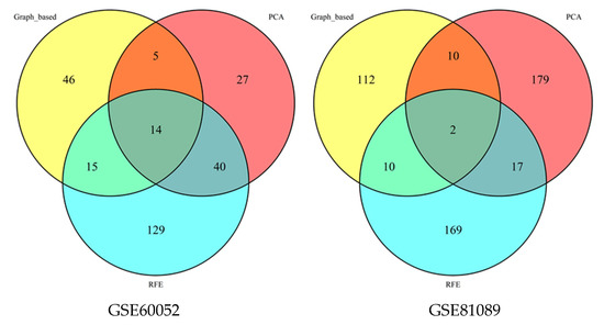
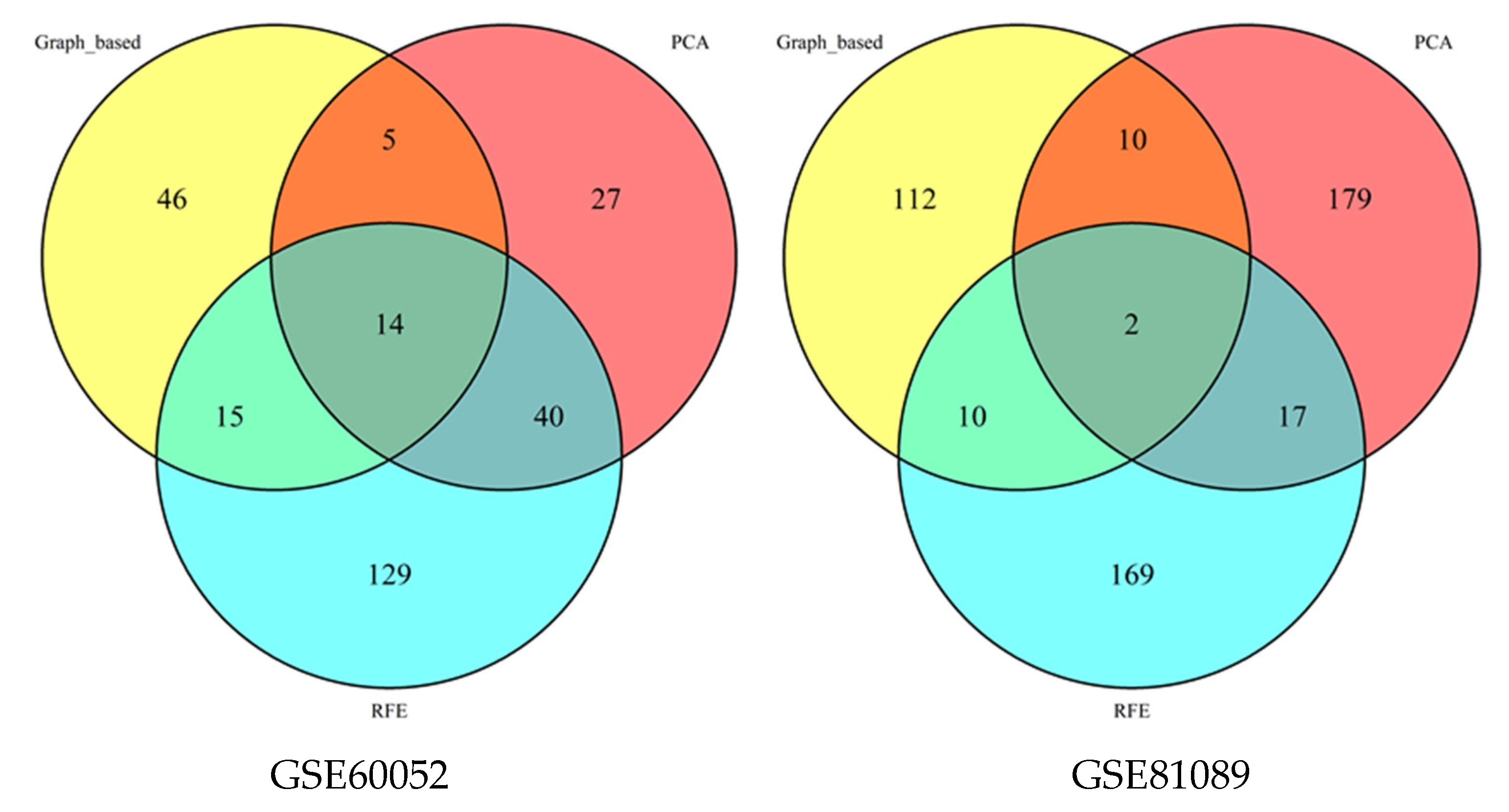
After preprocessing, we used three feature-selection approaches to filter the features further to retain only informative features. The RFE retained the highest number of features in both datasets followed by PCA as shown in Table 2 and Figure 1.

Figure 1. Features selected by each of the methods from the two datasets.

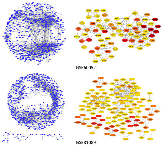
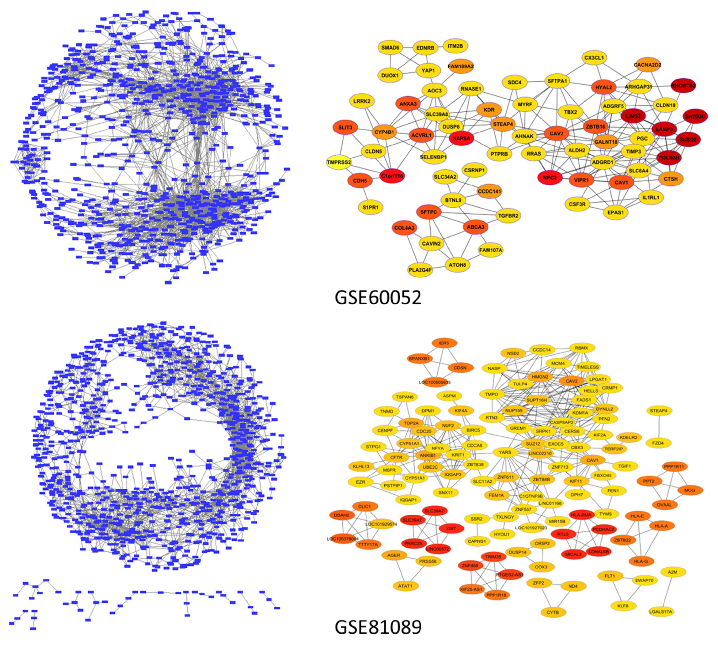
The graph-based feature-selection approach retained 80 for the SCLC dataset and 134 features for the NSCLC dataset. This is because the graph considers only the connecting features and the filtering step using maximal cliques retaining only the features that had the highest maximal clique score. Figure 2 presents the networks for the two datasets before and after filtering using maximal cliques.

Figure 2. Network diagrams for the 2 datasets: figures on the left side represent the network before filtering while those on the right show the networks after filtering with maximal clique. On the filtered networks, different colors denote expression levels with red color showing features that were highly expressed.

4.3. Classification

In the next step, we compared the performance of three classifiers with the features selected in the previous step as input while the raw features were our baseline. Table 3 summarizes the performance of the various classifiers before and after feature selection. The accuracy value, root mean squared error (RMSE), mean absolute error (MAE), kappa statistic (KS) and the time taken to build the model for every classifier, arising from the 10-fold cross validation are given. Overall, accuracy levels after selection ranged between 94.186 and 100% depending on the classification method used and the dataset (Table 3).

Table 3. Classification results after feature selection.

NAÏVE BAYES
Dataset	Feature Selection Method	Accuracy	MAE	Kappa	RMSE	F-Measure	T/s
GSE60052	Graph-based	96.4286	0.0357	0.8679	0.189	0.963	0.01
	RFE	100	0	1	0	1	0.01
	PCA	96.4286	0.0357	0.8679	0.189	0.963	0.02
GSE81089	Graph-based	100	0	1	0	1	0.06
	RFE	100	0	1	0	1	0.01
	PCA	100	0	1	0	1	0.02
MULTILAYER PERCEPTRON
Dataset	Feature Selection Method	Accuracy	MAE	Kappa	RMSE	F-Measure	T/s
GSE60052	Graph-based	96.4286	0.0366	0.8679	0.1814	0.979	18.66
	RFE	96.4286	0.0389	0.8679	0.1851	0.963	9.7
	PCA	96.4286	0.0224	0.8679	0.0993	0.963	9.62
GSE81089	Graph-based	96.4286	0.0389	0.8679	0.1851	0.963	124.15
	RFE	100	0	1	0	1	131.53
	PCA	100	0	1	0	1	0.77
SEQUENTIAL MINIMAL OPTIMIZATION
Dataset	Feature Selection Method	Accuracy	MAE	Kappa	RMSE	F-Measure	T/s
GSE60052	Graph-based	96.4286	0.0357	0.8679	0.189	0.889	0.01
	RFE	96.4286	0.0357	0.8679	0.189	0.963	0.01
	PCA	100	0	1	0	1	0.02
GSE81089	Graph-based	98.5915	0.0141	0.9567	0.1187	0.986	0.14
	RFE	100	0	1	0	1	0.01
	PCA	100	0	1	0	1	0.01

NB performed better on features selected using PCA and a graph-based approach whereby accuracy, MAE, kappa and time taken improved as compared to unfiltered features and RFE-selected features where there was no difference. This can be attributed to the working principle of RFE where the optimal number of features is not known apriori (in advance) [58]. A Kruskal–Wallis test showed that there is no significant difference between the mean ranks of the groups ($p<0.05$), i.e., 20 iterations for each of the feature-selection methods.

A study by Furat and Ibrikci [59] used five tumor types of gene expression cancer RNA-Seq data and, using Naïve Bayes with 10-fold cross validation, achieved an accuracy of 98.7516%. This shows that NB accuracy levels will vary with the dataset being analyzed. In dataset GSE81089, which had a larger sample size of selected features, SMO and MLP achieved 100% accuracy when feature selection was performed prior to classification, and in fact, the PCA-selected features could be classified at 100% accuracy by all three classifiers. In the smaller dataset, SCLC dataset, accuracy levels were also lower. Notable is that a graph-based feature-selection approach gave the best classification results in the two datasets and also took the least time to execute. The time required to build the model improved after feature selection across the three classifiers though MLP required the longest duration and a graph-based approach the shortest (Table 3).

4.4. Association Rule Mining

Features from PCA, RFE and graph-based selection methods were discretized and analyzed to find possible associations using Apriori. The resulting number of rules, maximum confidence, support and lift values are summarized in Table 4.

Table 4. Rules generated using Apriori from features selected using different approaches.

Dataset	Selection Method	Support	Confidence	Lift	No. of Rules	Non-Redundant Rules
GSE60052	Graph-based	0.5	0.9	2	19	15
	PCA	0.4	0.9	2	38	38
	RFE	0.3	0.9	1.98	357,986	112,357
GSE81089	Graph-based	0.5	0.9	2	36	36
	PCA	0.4	0.9	1	121	121
	RFE	0.4	0.9	1	899	884

The graph-based feature-selection approach gave 15 and 36 non-redundant rules, respectively, from the two datasets at a support of 0.5 confidence value of 0.9 and a lift of 2. The other feature-selection methods did not generate any rules at a support of 0.5. Features selected by RFE had the lowest maximum support and lift, and this led to the generation of too many redundant rules. For the PCA-based feature selection, support ranged between 0.405 and 0.425 with a total of 38 rules for the first dataset and 36 rules for the second dataset (Table 4). The top 10 rules are shown in Table 5.

Table 5. A summary of top ten rules generated from the two datasets after graph-based.

GSE60052
Rules		Support	Confidence	Lift
X	Y
{SFTPA1, SDC4, LRRK2} => {SLC34A2}		0.5	0.9	2
{ACVRL1, COL4A3, AQP1} => {SLC34A2}		0.5	0.9	2
{EDNRB, SFTPC, AGER} => {SLC34A2}		0.5	0.9	2
{PTPRB, SFTPC, CLDN5} => {SLC34A2}		0.5	0.9	2
{EPAS1, EDNRB, LRRK2, AQP1} => {SLC34A2}		0.5	0.9	2
{CLDN18, EPAS1, SFTPA1, AGER} => {SLC34A2}		0.5	0.9	2
{EPAS1, NAPSA, LRRK2, AGER} => {SLC34A2}		0.5	0.9	2
{TIMP3, CTSH, SFTPA1, LRRK2} => {SLC34A2}		0.5	0.9	2
{CTSH, NAPSA, TGFBR2, SFTPC} => {SLC34A2}		0.5	0.9	2
{RRAS, PTPRB, YAP1, SMAD6} => {SLC34A2}		0.5	0.9	2
GSE81089
Rules		Support	Confidence	Lift
X	Y
{ASPM, KIF4A, NUF2} => {CENPF}		0.5	1	2
{ASPM, KIF4A, CDC6, NUF2} => {TOP2A}		0.5	1	2
{ASPM, CDC6, CDC20, NUF2} => {TOP2A}		0.5	1	2
{ASPM, CDC6, CDCA8, NUF2} => {TOP2A}		0.5	1	2
{TPX2, FOXM1, NUF2, IQGAP3} => {BIRC5}		0.5	1	2
{CDC6, FOXM1, CDC20, UBE2C} => {TPX2}		0.5	1	2
{ASPM, CDC6, DLGAP5, NUF2} => {TOP2A}		0.5	1	2
{TPX2, CDCA8, UBE2C, IQGAP3} => {BIRC5}		0.5	1	2
{ASPM, KIF4A, CDC6, UBE2C} => {CENPF}		0.5	1	2
{TPX2, CDC6, FOXM1, IQGAP3} => {BIRC5}		0.5	1	2

Association rules are represented as X => Y, where X and Y are items contained within a dataset/database, and X ∩ Y = ø. X is the antecedent, and Y is the consequent (Table 5). It means that whenever X, which is the antecedent, is present, even Y, which is the consequent, will be present. Support indicates the frequency of the itemset appearance in the dataset, and the confidence indicates how often a rule has been found to be true. A support value of 0.5 means 50% of the items (genes) are found in the transaction and 90% of the rules are true (Confidence). The lower support means that most of the items are not frequently found together. The lift value is used to measure the rule importance. A lift of greater than 2 achieved by the graph-based feature-selection approach indicates the degree to which any two occurrences depend on each other, and this is an indication those rules are useful in consequent prediction.

External factors that play a critical role in the success of this type of study include the choice of the technology used in generating the data since it determines the volume and quality of the data across the replicates. The cost of generating the data also limits the number of samples as well as the volume of data. In the biological space, what can be defined as control/normal samples is a gray area, and therefore this may have a bearing on downstream analysis while at the same time bringing about class imbalance. Internal threats to this kind of study include experimental noise in the data as well as the assumption that gene expression level is uniform across cells. Co-regulation and co-expression between the features can also lead to redundancy in the datasets. Features without an assigned biological function may also not be informative unless in vitro experiments are designed to validate the function.

5. Conclusions

In this study, we used three different feature-selection methods to select informative features from two different cancer datasets. Most existing feature-selection techniques assume that features are independent of one another. However, this assumption ignores the fact that biological features are usually related because of their function in living systems. We evaluated the performance of three classifiers on the selected features. Features selected using a graph-based approach with maximal clique could be classified with high accuracy when compared to PCA and RFE. These features also gave informative rules with a higher support and lift as compared to those selected using PCA and RFE. Therefore, the proposed graph-based feature-selection approach combined with rule mining is a suitable way of selecting and finding associations between features in high-dimensional RNA-Seq data.

References

- Jindal, P.; Kumar, D. A review on dimensionality reduction techniques. Int. J. Comput. Appl. 2017, 173, 42–46. [Google Scholar] [CrossRef] [Scilit]
- Nguyen, L.H.; Holmes, S. Ten quick tips for effective dimensionality reduction. PLoS Comput. Biol. 2019, 15, e1006907. [Google Scholar] [CrossRef] [Scilit] [PubMed]
- Zebari, R.; Abdulazeez, A.; Zeebaree, D.; Zebari, D.; Saeed, J. A comprehensive review of dimensionality reduction techniques for feature selection and feature extraction. J. Appl. Sci. Technol. Trends 2020, 1, 56–70. [Google Scholar] [CrossRef] [Scilit]
- Abdulrazzaq, M.B.; Saeed, J.N. A Comparison of Three Classification Algorithms for Handwritten Digit Recognition. In Proceedings of the 2019 International Conference on Advanced Science and Engineering (ICOASE), Zakho-Duhok, Iraq, 2–4 April 2019; pp. 58–63. [Google Scholar]
- Mafarja, M.; Mirjalili, S. Whale optimization approaches for wrapper feature selection. Appl. Soft Comput. 2018, 62, 441–453. [Google Scholar] [CrossRef] [Scilit]
- Yu, L.; Liu, H. Feature Selection for High-Dimensional Data: A Fast Correlation-Based Filter Solution. In Proceedings of the 20th international conference on machine learning (ICML-03), Washington, DC, USA, 21–24 August 2003; pp. 856–863. [Google Scholar]
- Chandrashekar, G.; Sahin, F. A survey on feature selection methods. Comput. Electr. Eng. 2014, 40, 16–28. [Google Scholar] [CrossRef] [Scilit]
- Jović, A.; Brkić, K.; Bogunović, N. A review of feature selection methods with applications. In Proceedings of the 2015 38th International Convention on Information and Communication Technology, Electronics and Microelectronics (MIPRO), Opatija, Croatia, 25–29 May 2015; pp. 1200–1205. [Google Scholar]
- Mlambo, N.; Cheruiyot, W.K.; Kimwele, M.W. A survey and comparative study of filter and wrapper feature selection techniques. Int. J. Eng. Sci. 2016, 5, 57–67. [Google Scholar]
- Urbanowicz, R.J.; Meeker, M.; La Cava, W.; Olson, R.S.; Moore, J.H. Relief-based feature selection: Introduction and review. J. Biomed. Inform. 2018, 85, 189–203. [Google Scholar] [CrossRef] [Scilit]
- Abiodun, E.O.; Alabdulatif, A.; Abiodun, O.I.; Alawida, M.; Alabdulatif, A.; Alkhawaldeh, R.S. A systematic review of emerging feature selection optimization methods for optimal text classification: The present state and prospective opportunities. Neural Comput. Appl. 2021, 33, 15091–15118. [Google Scholar] [CrossRef] [Scilit]
- Piles, M.; Bergsma, R.; Gianola, D.; Gilbert, H.; Tusell, L. Feature Selection Stability and Accuracy of Prediction Models for Genomic Prediction of Residual Feed Intake in Pigs Using Machine Learning. Front. Genet. 2021, 12, 137. [Google Scholar] [CrossRef] [Scilit]
- Yang, P.; Huang, H.; Liu, C. Feature selection revisited in the single-cell era. Genome Biol. 2021, 22, 321. [Google Scholar] [CrossRef] [Scilit]
- Arowolo, M.O.; Adebiyi, M.O.; Adebiyi, A.A.; Olugbara, O. Optimized hybrid investigative based dimensionality reduction methods for malaria vector using KNN classifier. J. Big Data 2021, 8, 1–14. [Google Scholar] [CrossRef] [Scilit]
- Cateni, S.; Vannucci, M.; Vannocci, M.; Colla, V. Variable Selection and Feature Extraction through Artificial Intelligence Techniques. Available online: https://www.intechopen.com/chapters/41752 (accessed on 7 December 2021).
- Kim, K. An improved semi-supervised dimensionality reduction using feature weighting: Application to sentiment analysis. Expert Syst. Appl. 2018, 109, 49–65. [Google Scholar] [CrossRef] [Scilit]
- Samuel, A.L. Some studies in machine learning using the game of checkers. IBM J. Res. Dev. 1959, 3, 210–229. [Google Scholar] [CrossRef] [Scilit]
- Das, H.; Naik, B.; Behera, H. Classification of diabetes mellitus disease (DMD): A data mining (DM) approach. In Progress in Computing, Analytics and Networking; Springer: Singapore, 2018; pp. 539–549. [Google Scholar]
- Mazumder, D.H.; Veilumuthu, R. An enhanced feature selection filter for classification of microarray cancer data. ETRI J. 2019, 41, 358–370. [Google Scholar] [CrossRef] [Scilit]
- Sun, S.; Zhu, J.; Ma, Y.; Zhou, X. Accuracy, robustness and scalability of dimensionality reduction methods for single-cell RNA-seq analysis. Genome Biol. 2019, 20, 1–21. [Google Scholar] [CrossRef] [Scilit]
- Ai, D.; Pan, H.; Li, X.; Gao, Y.; He, D. Association rule mining algorithms on high-dimensional datasets. Artif. Life Robot. 2018, 23, 420–427. [Google Scholar] [CrossRef] [Scilit]
- Agrawal, R.; Imieliński, T.; Swami, A. Mining Association Rules between Sets of Items in Large Databases. In Proceedings of the 1993 ACM SIGMOD international conference on Management of Data, Washington, DC, USA, 25–28 May 1993; pp. 207–216. [Google Scholar]
- Liu, X.; Sang, X.; Chang, J.; Zheng, Y.; Han, Y. The water supply association analysis method in Shenzhen based on kmeans clustering discretization and apriori algorithm. PLoS ONE 2021, 16, e0255684. [Google Scholar] [CrossRef] [Scilit]
- Saeys, Y.; Inza, I.; Larrañaga, P. A review of feature selection techniques in bioinformatics. Bioinformatics 2007, 23, 2507–2517. [Google Scholar] [CrossRef] [Scilit]
- Ang, J.C.; Mirzal, A.; Haron, H.; Hamed, H.N.A. Supervised, unsupervised, and semi-supervised feature selection: A review on gene selection. IEEE/ACM Trans. Comput. Biol. Bioinform. 2016, 13, 971–989. [Google Scholar] [CrossRef] [Scilit]
- Ray, R.B.; Kumar, M.; Rath, S.K. Fast In-Memory Cluster Computing of Sizeable Microarray Using Spark. In Proceedings of the 2016 International Conference on Recent Trends in Information Technology (ICRTIT), Chennai, India, 8–9 April 2016; pp. 1–6. [Google Scholar]
- Lokeswari, Y.; Jacob, S.G. Prediction of child tumours from microarray gene expression data through parallel gene selection and classification on spark. In Computational Intelligence in Data Mining; Springer: Singapore, 2017; pp. 651–661. [Google Scholar]
- Peralta, D.; Del Río, S.; Ramírez-Gallego, S.; Triguero, I.; Benitez, J.M.; Herrera, F. Evolutionary feature selection for big data classification: A mapreduce approach. Math. Probl. Eng. 2015, 2015. [Google Scholar] [CrossRef] [Scilit]
- Sonnenburg, S.; Franc, V.; Yom-Tov, E.; Sebag, M. Pascal Large Scale Learning Challenge. In Proceedings of the 25th International Conference on Machine Learning (ICML2008) Workshop, Helsinki, Finland, 5–9 July 2008. [Google Scholar]
- Alghunaim, S.; Al-Baity, H.H. On the scalability of machine-learning algorithms for breast cancer prediction in big data context. IEEE Access 2019, 7, 91535–91546. [Google Scholar] [CrossRef] [Scilit]
- Turgut, S.; Dağtekin, M.; Ensari, T. Microarray Breast Cancer Data Classification Using Machine Learning Methods. In Proceedings of the 2018 Electric Electronics, Computer Science, Biomedical Engineerings’ Meeting (EBBT), Istanbul, Turkey, 18–19 April 2018. [Google Scholar]
- Matamala, N.; Vargas, M.T.; Gonzalez-Campora, R.; Minambres, R.; Arias, J.I.; Menendez, P.; Andres-Leon, E.; Gomez-Lopez, G.; Yanowsky, K.; Calvete-Candenas, J. Tumor microRNA expression profiling identifies circulating microRNAs for early breast cancer detection. Clin. Chem. 2015, 61, 1098–1106. [Google Scholar] [CrossRef] [Scilit]
- Morovvat, M.; Osareh, A. An ensemble of filters and wrappers for microarray data classification. Mach. Learn. Appl. An. Int. J. 2016, 3, 1–17. [Google Scholar] [CrossRef] [Scilit]
- Goswami, S.; Das, A.K.; Guha, P.; Tarafdar, A.; Chakraborty, S.; Chakrabarti, A.; Chakraborty, B. An approach of feature selection using graph-theoretic heuristic and hill climbing. Pattern Anal. Appl. 2019, 22, 615–631. [Google Scholar] [CrossRef] [Scilit]
- Zhang, Z.; Hancock, E.R. A Graph-Based Approach to Feature Selection. In International Workshop on Graph-Based Representations in Pattern Recognition; Springer: Berlin/Heidelberg, Germany, 2011; pp. 205–214. [Google Scholar]
- Schroeder, D.T.; Styp-Rekowski, K.; Schmidt, F.; Acker, A.; Kao, O. Graph-Based Feature Selection Filter Utilizing Maximal Cliques. In Proceedings of the 2019 Sixth International Conference on Social Networks Analysis, Management and Security (SNAMS), Granada, Spain, 22–25 October 2019; pp. 297–302. [Google Scholar]
- Roffo, G.; Castellani, U.; Vinciarelli, A.; Cristani, M. Infinite feature selection: A graph-based feature filtering approach. IEEE Trans. Pattern Anal. Mach. Intell. 2020, 43, 12. [Google Scholar] [CrossRef] [Scilit]
- Rana, P.; Thai, P.; Dinh, T.; Ghosh, P. Relevant and Non-Redundant Feature Selection for Cancer Classification and Subtype Detection. Cancers 2021, 13, 4297. [Google Scholar] [CrossRef] [Scilit]
- Nguyen, H.; Thai, P.; Thai, M.; Vu, T.; Dinh, T. Approximate k-Cover in Hypergraphs: Efficient Algorithms, and Applications. arXiv 2019, arXiv:1901.07928. [Google Scholar]
- Lu, S.J.; Xie, J.; Li, Y.; Yu, B.; Ma, Q.; Liu, B.Q. Identification of lncRNAs-gene interactions in transcription regulation based on co-expression analysis of RNA-seq data. Math. Biosci. Eng. 2019, 16, 7112–7125. [Google Scholar] [CrossRef] [Scilit]
- Chiclana, F.; Kumar, R.; Mittal, M.; Khari, M.; Chatterjee, J.M.; Baik, S.W. ARM–AMO: An efficient association rule mining algorithm based on animal migration optimization. Knowl. Based Syst. 2018, 154, 68–80. [Google Scholar]
- Wen, F.; Zhang, G.; Sun, L.; Wang, X.; Xu, X. A hybrid temporal association rules mining method for traffic congestion prediction. Comput. Ind. Eng. 2019, 130, 779–787. [Google Scholar] [CrossRef] [Scilit]
- Shui, Y.; Cho, Y.-R. Filtering Association Rules in GENE Ontology Based on Term Specificity. In Proceedings of the 2016 IEEE international conference on bioinformatics and biomedicine (bibm), Shenzhen, China, 15–18 December 2016; pp. 1314–1321. [Google Scholar]
- Agapito, G.; Cannataro, M.; Guzzi, P.H.; Milano, M. Using GO-WAR for mining cross-ontology weighted association rules. Comput. Methods Programs Biomed. 2015, 120, 113–122. [Google Scholar] [CrossRef] [Scilit] [PubMed]
- Bhavsar, H.; Ganatra, A. A comparative study of training algorithms for supervised machine learning. Int. J. Soft Comput. Eng. (IJSCE) 2012, 2, 2231–2307. [Google Scholar]
- Han, J.; Pei, J.; Kamber, M. Data Mining: Concepts and Techniques; The Morgan Kaufmann Series in Data Management Systems 5.4; Morgan Kaufmann Publishers: Waltham, MA, USA, 2011; pp. 83–124. [Google Scholar]
- Hall, M.; Frank, E.; Holmes, G.; Pfahringer, B.; Reutemann, P.; Witten, I.H. The WEKA data mining software: An update. ACM SIGKDD Explor. Newsl. 2009, 11, 10–18. [Google Scholar] [CrossRef] [Scilit]
- Vapnik, V.N. An overview of statistical learning theory. IEEE Trans. Neural Netw. 1999, 10, 988–999. [Google Scholar] [CrossRef] [Scilit]
- Tanwani, A.K.; Afridi, J.; Shafiq, M.Z.; Farooq, M. Guidelines to Select Machine Learning Scheme for Classification of Biomedical Datasets. In Proceedings of the European Conference on Evolutionary Computation, Machine Learning and Data Mining in Bioinformatics; Springer: Berlin/Heidelberg, Germany, 2009; pp. 128–139. [Google Scholar]
- Carletta, J. Assessing agreement on classification tasks: The kappa statistic. arXiv 1996, arXiv:9602004. [Google Scholar]
- Chai, T.; Draxler, R.R. Root mean square error (RMSE) or mean absolute error (MAE)?—Arguments against avoiding RMSE in the literature. Geosci. Model Dev. 2014, 7, 1247–1250. [Google Scholar] [CrossRef] [Scilit]
- Dunham, M.H.; Sridhar, S. Data Mining: Introductory and Advanced Topics, Dorling Kindersley; Pearson Education: New Delhi, India, 2006. [Google Scholar]
- Jiang, L.; Huang, J.; Higgs, B.W.; Hu, Z.; Xiao, Z.; Yao, X.; Conley, S.; Zhong, H.; Liu, Z.; Brohawn, P. Genomic landscape survey identifies SRSF1 as a key oncodriver in small cell lung cancer. PLoS Genet. 2016, 12, e1005895. [Google Scholar] [CrossRef] [Scilit]
- Djureinovic, D.; Hallström, B.M.; Horie, M.; Mattsson, J.S.M.; La Fleur, L.; Fagerberg, L.; Brunnström, H.; Lindskog, C.; Madjar, K.; Rahnenführer, J. Profiling cancer testis antigens in non–small-cell lung cancer. JCI Insight 2016, 1, e86837. [Google Scholar] [CrossRef] [Scilit]
- Bullard, J.; Purdom, E.; Hansen, K.D.; Dudoit, S. Evaluation of statistical methods for normalization and differential expression in mrna-seq experiments. BMC Bioinform. 2010, 11, 94. [Google Scholar] [CrossRef] [Scilit]
- Ustebay, S.; Turgut, Z.; Aydin, M.A. Intrusion Detection System with Recursive Feature Elimination by Using Random Forest and Deep Learning Classifier. In Proceedings of the International Congress on Big Data, Deep Learning and Fighting Cyber Terrorism (IBIGDELFT), Ankara, Turkey, 3–4 December 2018; pp. 71–76. [Google Scholar]
- Gunduz, H. An efficient stock market prediction model using hybrid feature reduction method based on variational autoencoders and recursive feature elimination. Financ. Innov. 2021, 7, 1–24. [Google Scholar] [CrossRef] [Scilit]
- Artur, M. Review the performance of the Bernoulli Naïve Bayes Classifier in Intrusion Detection Systems using Recursive Feature Elimination with Cross-validated selection of the best number of features. Procedia Comput. Sci. 2021, 190, 564–570. [Google Scholar] [CrossRef] [Scilit]
- Furat, F.G.; İbrikçi, T. Tumor Type Detection Using Naïve Bayes Algorithm on Gene Expression Cancer RNA-Seq Data Set. Lung Cancer 2019, 10, 13. [Google Scholar]
Publisher’s Note: MDPI stays neutral with regard to jurisdictional claims in published maps and institutional affiliations. |
© 2022 by the authors. Licensee MDPI, Basel, Switzerland. This article is an open access article distributed under the terms and conditions of the Creative Commons Attribution (CC BY) license (https://creativecommons.org/licenses/by/4.0/).