Fault Diagnosis for Active Distribution Network Based on Colored and Fuzzy Colored Petri Net

Abstract

Accurate and rapid fault diagnosis is critical for active distribution networks characterized by growing structural complexity and diverse load profiles. This paper proposes a two-stage fault diagnosis framework that synergistically combines colored Petri nets (CPN) and fuzzy colored Petri nets (FCPN). In the first stage, a CPN fault zone search model employing a breadth-first search (BFS) strategy is developed to identify suspected faulty components by processing circuit breaker operation information and grid topology. In the second stage, an FCPN diagnosis model is constructed by extending hierarchical fuzzy Petri nets through color assignment to confidence tokens. A key feature of this model is a dedicated initial confidence assessment module that dynamically evaluates the reliability of protection and circuit breaker actions by synthesizing device self-check alarms and operational timing information, thereby overcoming the limitation of empirical, static confidence assignment in existing methods. The resulting initial confidence values are then propagated through a hierarchical confidence inference module to determine the fault likelihood of each suspected component. Comparative simulations across four fault scenarios demonstrate that the proposed method achieves higher diagnostic accuracy and stronger fault tolerance than state-of-the-art approaches, correctly identifying all faulty components even under degraded alarm conditions.

1. Introduction

The integration of renewable energy generation and flexible loads has significantly increased the complexity of distribution network structures. Consequently, developing rapid and accurate fault diagnosis methods is of paramount importance for ensuring the secure operation of active distribution networks [1,2]. Currently, common fault diagnosis methods for power grids include expert systems [3], artificial neural networks [4,5], Bayesian network [6], analytical models [7,8], and Petri nets [9,10]. However, each of these methods has inherent limitations: expert systems heavily rely on expert experience, and maintaining their knowledge base is difficult; artificial neural networks lack interpretability of diagnostic results, and retraining is required when the grid topology changes, making it hard to ensure the completeness of the sample set; the Bayesian network faces difficulties in modeling and obtaining prior probabilities for complex grid structures; analytical models usually have high computational complexity and subjective weight allocation; the Petri net method is simple and intuitive, but it is not well-suited to handle uncertain events in the power grid.

Fuzzy Petri nets (FPN) have been developed to mitigate the limitations of traditional Petri nets. Ref. [11] proposes a weighted FPN based on fault propagation directions, demonstrating good adaptability to adjustments in power grid topologies; Ref. [12] integrates temporal constraints to enhance the fault tolerance of FPN diagnostic models; Ref. [13] addresses uncertainty in alarm information by employing intuitionistic fuzzy sets to represent certainty and uncertainty; Ref. [14] modifies place confidence using Gaussian functions based on time-constrained hierarchical fuzzy Petri nets; Ref. [15] designs a hierarchical FPN with confidence-time synchronized reasoning, significantly improving diagnostic accuracy. Despite these advancements, the aforementioned FPN diagnosis models depend on the offline analysis to determine the initial confidence levels for protections and circuit breaker actions. Furthermore, these diagnostic methods rely predominantly on action information and timing data from protections and circuit breakers, which limits the richness and robustness of the information utilized.

Microprocessor-based protection in power systems can directly monitor the status of internal protection components. When abnormal protection or circuit breaker operations occur, or when false alarms or missed alarms are generated, the dispatch center receives self-check alarm information through self-diagnostic technology [16]. Leveraging these self-check data from protection devices and circuit breakers, Ref. [17] constructed a multi-objective optimization model incorporating the reliability of operational status information, further improving both the speed and accuracy of fault diagnosis.

Furthermore, the proliferation of distributed energy resources within active distribution networks introduces greater topological complexity and dynamic load behavior, rendering traditional network topology analysis methods inadequate for fault zone identification. Refs. [8,18] employ breadth-first search (BFS) to rapidly identify fault zone boundaries based on post-fault electrical quantities and circuit breaker position changes. The modeling principles of colored Petri nets (CPN) for flexible manufacturing systems also provide reliable insights for determining fault zones in active distribution networks [19].

This paper proposes a fault diagnosis method for active distribution networks that synergistically combines CPN and fuzzy colored Petri nets (FCPN). First, a CPN fault zone search model is developed, rapidly identifying suspected faulty components based on circuit breaker operation information and grid topology. In the second stage, a modular FCPN diagnostic model for suspected faulty components is constructed, which is achieved by extending hierarchical FPN through assigning confidence tokens colors. The FCPN model evaluates the initial confidence of protections and circuit breakers by synthesizing self-check and timing information. The results from this assessment module are then fed into a confidence inference module, which performs hierarchical reasoning to determine the fault confidences of suspicious components. Through extensive comparative simulations of multiple case studies, the proposed fault diagnosis method achieves high diagnostic accuracy while maintaining strong fault tolerance.

The model construction and simulation examples in this paper were both completed on the CPN IDE platform, with the functions in the model defined using the ML programming language [20].

The remainder of this paper is organized as follows. Section 2 introduces CPN and FCPN foundations and the test network topology. Section 3 presents the BFS-based CPN fault zone search model, showing how self-check alarm data is incorporated as a boundary condition for reliable fault zone delineation. Section 4 constructs the FCPN diagnosis model, with the initial confidence assessment module—the core innovation—synthesizing self-check and timing information to replace empirical assignment, followed by the hierarchical confidence inference module. Section 5 reports comparative case studies, and Section 6 concludes the paper.

2. Preliminaries

2.1. Colored Petri Net (CPN)

As an advanced extension form of the classic Petri net, the colored Petri net (CPN) assigns colors to tokens, thereby endowing them with additional attributes that can distinguish different types of resources in complex systems [21]. A CPN is formally defined as a 8-tuple: $CPN=(P,R,F,C,I,O,G,M_0)$, where

• $(P,R,F)$ is a basic Petri net, where $P=\{p_1,p_2,\dots ,p_n\}$ is a finite set of places, $R=\{r_1,r_2,\dots ,r_n\}$ is a finite set of transitions, and $F=(P\times R)\cup (R\times P)$ is the arc set of the net.
• C is the color set, which defines the type and attribute of tokens stored in the place. Tokens come in two types: monochrome and composite color. Monochrome tokens are represented as $n_1^{\prime }d$, where $n_1$ denotes the number of tokens and d denotes the monochrome attribute. Composite color tokens are represented as $n_2^{\prime }(d_1,d_2,\dots ,d_m)$, where $n_2$ denotes the number of tokens and $(d_1,d_2,\dots ,d_m)$ denotes the composite color attribute, which is a tuple composed of m monochrome attributes: $d_1,d_1,\dots ,d_m$.
• I is an expression on the input arc from the place to the transition, representing a finite number of tokens $i_1^{\prime }d$ or $i_2^{\prime }(d_1,d_2,\dots ,d_m)$ from the input place, where $i_1,i_2$ denotes the number of tokens and $d,(d_1,d_2,\dots ,d_m)$ denotes the token attributes.
• O is an expression on the output arc from the transition to the place, representing a finite number of tokens conforming to the token type and attributes of the output place, or a function $f(d_1,d_2,\dots ,d_s)$ whose result conforms to the token type and attributes of the output place, where f is the function name, and $d_1,d_1,\dots ,d_s$ are token attributes in the input expression I.
• G is a guard function that defines the preconditions for firing a transition. G returns a BOOL value; when the result is true, the transition is allowed to fire.
• $M_0$ denotes the initial state (marking). $M_0\left(p_i\right)$ represents the number of tokens in the place $p_i$ under the initial marking.

For $x\in P\cup R$, ${}^{·}x=\{y\mid y\in P\cup R\wedge (y,x)\in F\}$ is called the pre-set of x. For CPN, when there is no guard function on transition r, the fire condition for r is $\forall p\in {}^{·}r,M\left(p\right)\ge I(p,r)$; when there is a guard function on r, r is fired only if the guard function evaluates to true in addition to the aforementioned conditions.

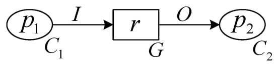
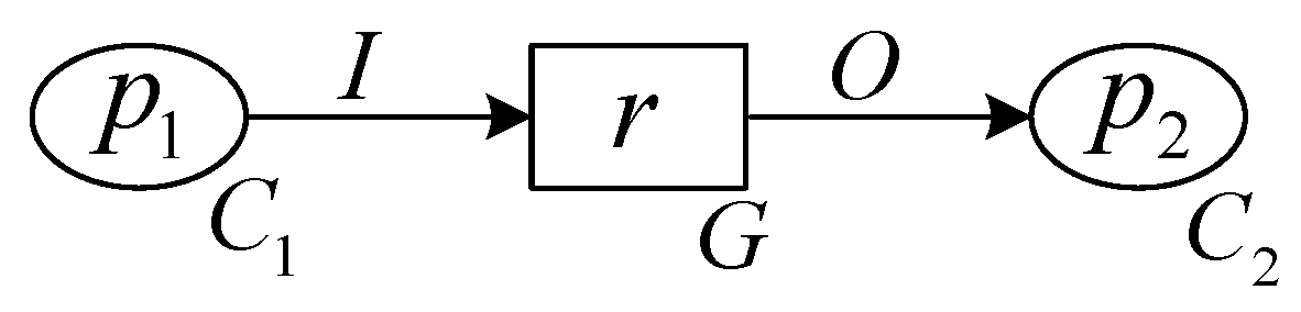
A simple CPN model is shown in Figure 1, where $C_1$ and $C_2$ denote the color sets corresponding to the place $p_1$ and $p_2$, respectively. G is the guard function for transition r, I is the input expression from $p_1$ to r, and O is the output expression from r to $p_2$.

Figure 1. A simple CPN model.

2.2. Fuzzy Colored Petri Net (FCPN)

In hierarchical fuzzy Petri nets, tokens are real numbers on the interval [0, 1], representing the confidence level of the propositions associated with their respective places. Building upon the CPN framework, this paper assigns colors to confidence tokens within hierarchical fuzzy Petri nets, thereby proposing a fuzzy colored Petri net (FCPN). A FCPN is formally defined as a 9-tuple: $FCPN=(P,R,F,C,I,O,W,Th,M_0)$, where

• The definitions of $P,R,F,C,I,O$ and $M_0$ are identical to those of CPN.
• $W=\{w_1,w_2,\dots ,w_n\}\cup \{u_1,u_2,\dots ,u_m\}$ is the weight set for input and output expressions. $w_1,w_2,\dots ,w_n$ are the weight set for input expression I. $u_1,u_2,\dots ,u_m$ are the weight set for output expression O.
• $Th$ is the threshold corresponding to the transition.

For transition r, the enabling condition requires that the weighted cumulative sum of confidence tokens from its input places meets or exceeds this threshold. To facilitate subsequent modeling operations on the CPN IDE platform, the following function equivalent to $Th$ is provided:

$$H\left(x\right)=\left\{\begin{array}{cc}0,\hfill & x<th\hfill \\ x,\hfill & x\ge th\hfill \end{array}\right.$$

(1)

where x represents the weighted cumulative sum of input confidence, and $th$ is a real number in the interval [0, 1], denoting the threshold value.

For FCPN, the fire condition for the transition r is $\forall p\in {}^{·}r,M\left(p\right)\ge I(p,r)$.

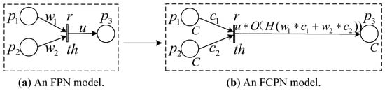
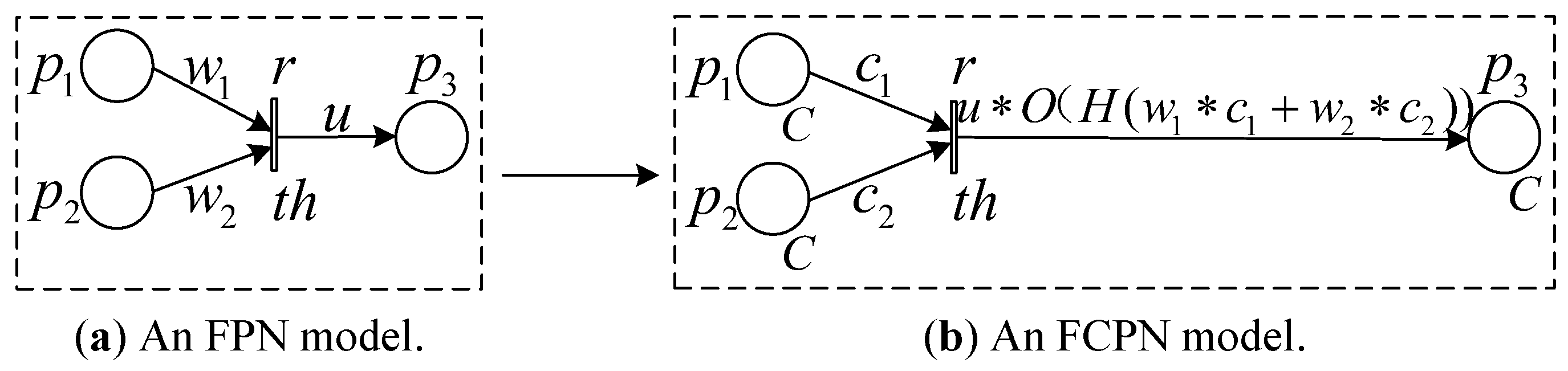
Figure 2a depicts a simplified hierarchical FPN model, where $w_1$ and $w_2$ represent the weights of input confidence from places $p_1$ and $p_2$, respectively, u denotes the weight of output confidence from transition r to place $p_3$, and $th$ is the threshold for r.

Figure 2. A hierarchical FPN and the corresponding FCPN model.

The corresponding FCPN model derived from this structure is shown in Figure 2b. The color set C specifies that the place $p_1,p_2$, and $p_3$ all hold confidence tokens. $c_1$ and $c_2$ represent the input confidence from $p_1$ and $p_2$, respectively. $w_1$ and $w_2$ are the weights for $c_1$ and $c_2$, respectively. H is the equivalence function for the transition r threshold, O is the output function, and u is the weight for O. After r fires, the output confidence obtained from the expression on the output arc in the diagram is stored in $p_3$.

2.3. Typical Active Distribution Network

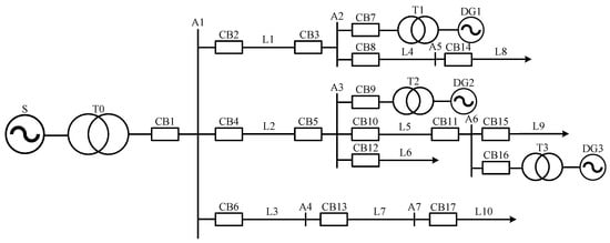
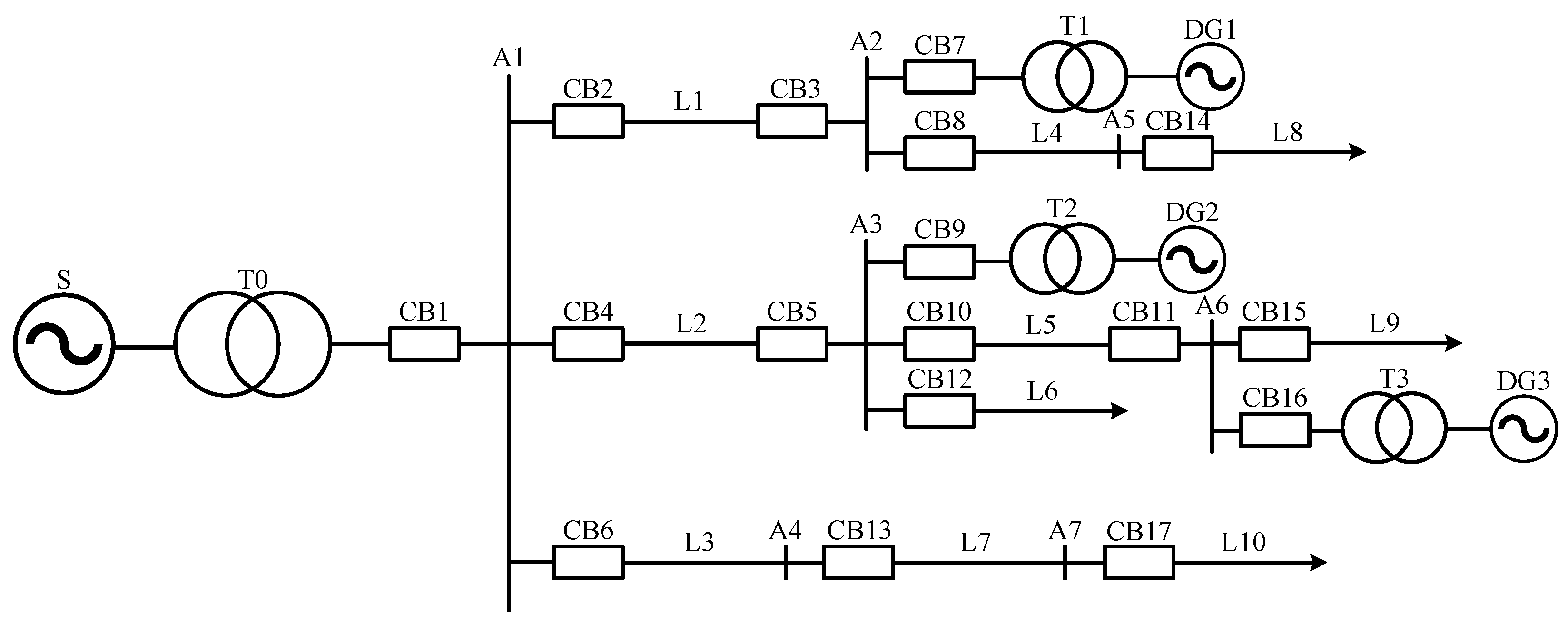
A typical active distribution network system architecture [22] is shown in Figure 3. In this diagram, S represents the main power source, DG1–DG3 denote distributed generation units, T0–T3 indicate transformers, CB1–CB17 signify circuit breakers, A1–A7 denote busbars, and L1–L10 represent power lines.

Figure 3. System structure of an active distribution network.

All lines in this active distribution network are equipped with main protection, near-backup protection, and far-backup protection. For lines downstream of the main power source and distributed power sources, a single-side protection is installed near the power source side, following traditional distribution network practices. For lines upstream of distributed power sources, a protection is installed on both sides of the line. All busbars in the distribution network are equipped with corresponding main protections. Transformers utilize integrated main and backup protection devices, where main protections and backup protections are not distinguished and are unified as a single category of protection [23].

3. CPN Fault Zone Search Model

When conducting fault diagnosis for the active distribution network, it is usually necessary to first search for the fault zones within the distribution network to identify the suspected faulty components, and then conduct diagnostic analysis targeting the suspected components. CPN has great application potential in power grid fault diagnosis due to its unique advantage of distinguishing different types of information using colors [24]. Moreover, applying the BFS strategy to perform fault zone search avoids full-network topological analysis as in traditional methods, thereby improving computational efficiency. Accordingly, this section proposes a CPN model based on the BFS strategy to achieve the search for the fault zones in the active distribution network.

3.1. CPN Model Design

A circuit breaker equipped with single-side protection will only trip normally due to a fault on that line or the downstream line. Therefore, research on determining fault zones in active distribution networks primarily focuses on scenarios involving multiple circuit breaker trips on lines with double-side protection.

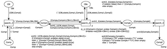
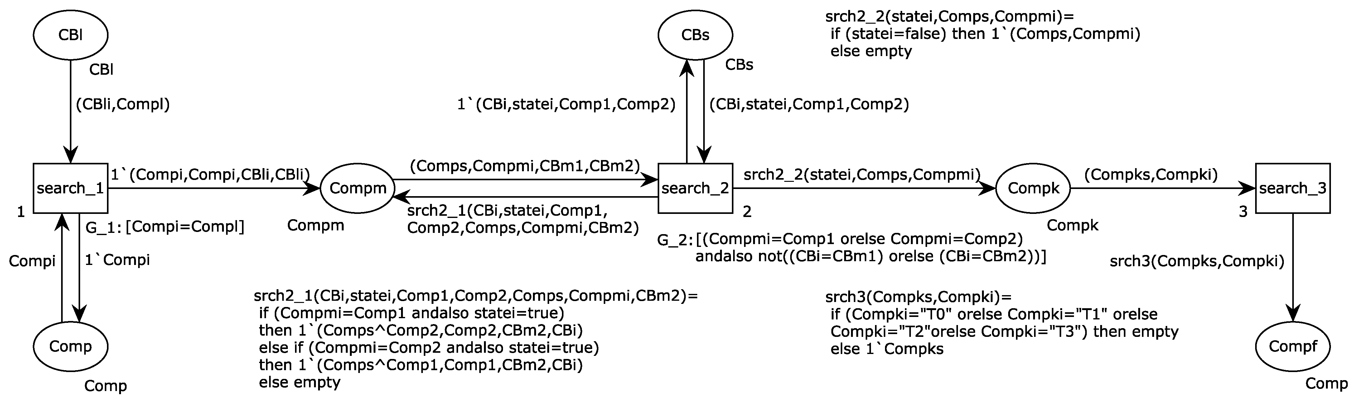
A complete path is defined as a set of adjacent components in the power grid connected by closed circuit breakers. All components along this path are arranged sequentially into a complete component sequence. A complete sequence that contains no active components such as transformers or power sources is termed a passive path component sequence. Based on the BFS method for searching fault zones, this paper develops the active distribution network CPN fault zone search model shown in Figure 4.

Figure 4. CPN fault zone search model for active distribution networks.

The CPN fault zone search model operates by inferring all possible passive path component sequences. It initiates the search from the components adjacent to a tripped circuit breaker and utilizes both the real-time breaker status information and the static network topology to trace connected paths, ultimately identifying the potential fault zones. By constructing a CPN fault zone search model, the visualization and integration of the fault area search process can be achieved. This not only makes the reasoning process clearer and more intuitive, but also facilitates the real-time update and maintenance of alarm information and the power grid topology.

According to the relevant definitions of component sequences and the search logic of the BFS method presented above, the model’s color sets, token types, and attributes are formally defined in Table 1 and Table 2, respectively. Among them, the operation state of circuit breakers is read as a BOOL value. For circuit breakers involved in alarms, their operation states are set to false; for those not involved, their operation states are set to true.

Table 1. Color sets for the CPN model in Figure 4.

Color Set Definition	Representation Content
Comp = string	Grid components or passive path component sequences.
CB = string	Circuit breakers in the power grid.
CBl = product CB*Comp	A tuple consisting of a tripped circuit breaker and its adjacent components.
Compm = product Comp*Comp*CB*CB	A tuple consisting of a component sequence and the adjacent circuit breaker of its terminal component.
CBs = product CB*BOOL*Comp*Comp	A tuple composed of the on/off state of a circuit breaker and its adjacent components.
Compk = product Comp*Comp	A tuple consisting of a complete component sequence and its terminal component.

Table 2. Token types and attributes of the CPN model in Figure 4.

Token Types and Attributes	Representation Content
Compi:Comp	A component of the power grid.
(CBli, Compl):CBl	$CBli$ denotes the tripped circuit breaker; $Compl$ denotes the adjacent component of that circuit breaker.
(Comps, Compmi, CBm1, CBm2):Compm	$Comps$ represents a component sequence currently found in a search; $Compmi$ indicates the terminal component of this sequence; $CBm1$ and $CBm2$ denote the adjacent circuit breakers of this terminal component.
(CBi, statei, Comp1, Comp2):$CBs$	$CBi$ denotes a circuit breaker; $statei$ is a BOOL variable indicating true/false for the breaker’s closed/open state; $Comp1$ and $Comp2$ denote the adjacent components of this circuit breaker.
(Compks, Compki):Compk	$Compks$ denotes a complete component sequence; $Compki$ denotes the terminal component of that sequence.

$G\_1$ and $G\_2$ are the guard functions for transitions $search\_1$ and $search\_2$, respectively. $srch2\_1$, $srch2\_2$, and $srch3$ are the functions on the output arcs for transition $search\_2$ to place $Compm$, $search\_2$ to place $Compk$, and $search\_3$ to place $Compf$, respectively. The descriptions of these functions are shown in Table 3.

Table 3. Functions of the CPN model in Figure 4.

Function Name	Function Description
$G\_1$	Determine whether $Compl$ and $Compi$ are identical.
$G\_2$	Determine whether $Compmi$ is equal to $Compl$ or $Comp2$, and determine whether $CBi$ is different from $CBm1$ and $CBm2$, thereby establishing the search direction.
$srch2\_1$	When $statei$ = true, pass the component sequence currently found in a search to the place $Compm$ in the form of token type defined by the color set $Compm$.
$srch2\_2$	When $statei$ = false, pass the complete component sequence currently found in a search to the place $Compk$ in the form of token type defined by color set $Compk$.
$srch3$	Pass the passive path component sequence to the place $Compf$ in the form of token type defined by color set $Comp$.

3.2. Search Algorithm and Process

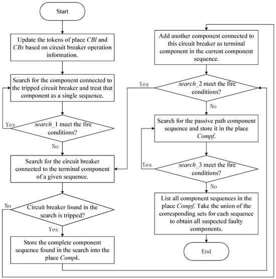
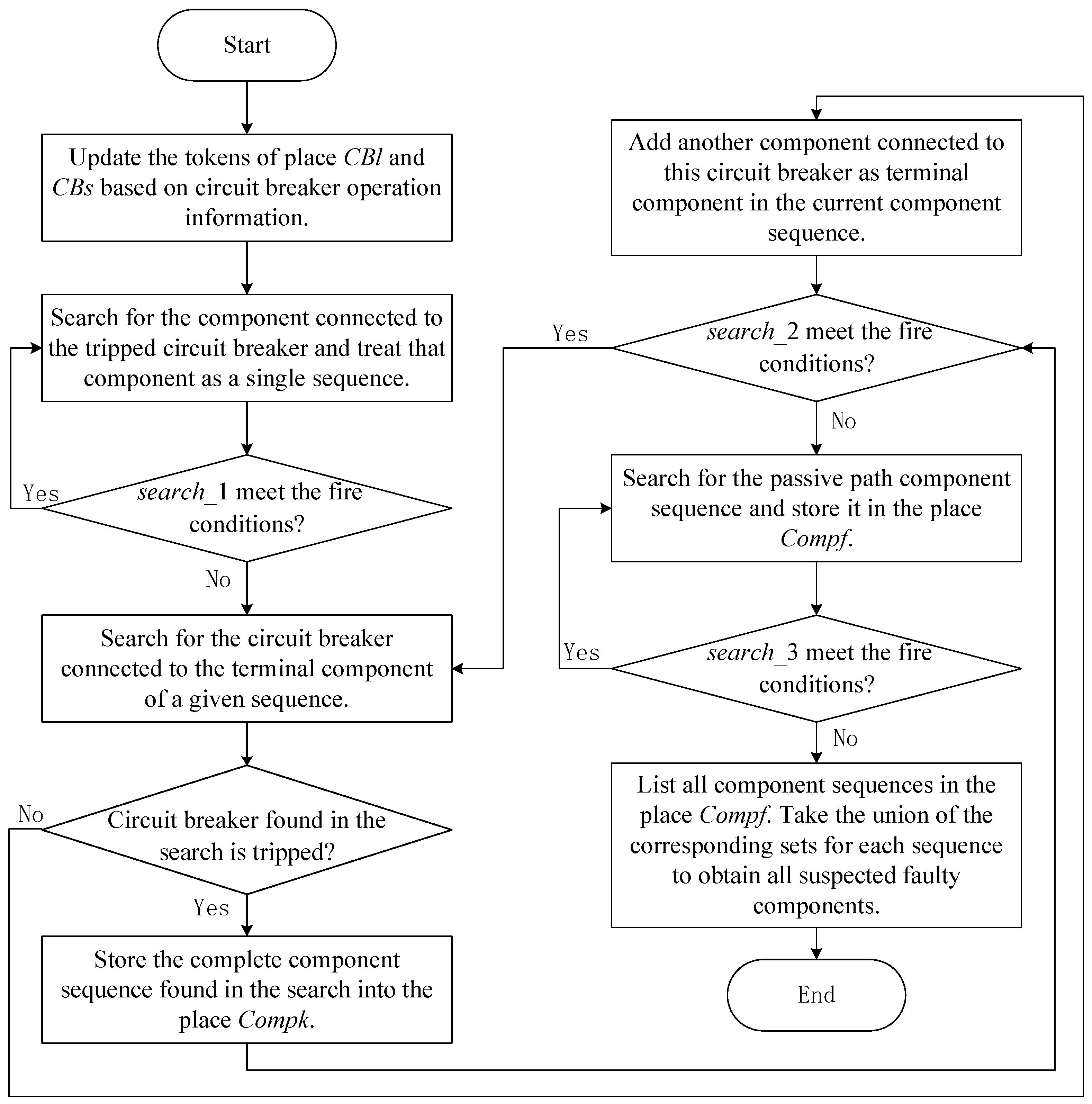
For a given active distribution network, tokens conforming to the color set are pre-assigned to the place $Comp$ and $CBs$ based on the network topology. Upon a fault occurrence, the model advances the search for the fault zones by firing transitions $search\_1$, $search\_2$, and $search\_3$, as depicted in the flowchart in Figure 5. The firing sequence is strictly defined: first, $search\_1$ is fired repeatedly until no longer enabled; then, $search\_2$ is fired under the same condition; finally, $search\_3$ is fired. Upon completion of this firing sequence, passive path component sequences accumulated in place $Compf$ constitutes the fault zones.

Figure 5. Fault zone searching flow diagram of CPN model.

3.3. Case

Based on the grid topology in Figure 3, tokens are pre-assigned to the place $Comp$ and $CBs$. When the dispatch center receives alarms indicating that circuit breakers CB5, CB9, and CB11 have been triggered:

• Update the tokens in the place $CBl$ and $CBs$ to obtain the initial marking $M_0$ for the model. For $CBl$, $M_0\left(CBl\right)=1^{\prime }\left(\mathrm{CB}5,\mathrm{L}2\right)+1^{\prime }\left(\mathrm{CB}5,\mathrm{A}3\right)+1^{\prime }\left(\mathrm{CB}9,\mathrm{A}3\right)+1^{\prime }\left(\mathrm{CB}9,\mathrm{T}2\right)+1^{\prime }\left(\mathrm{CB}11,\mathrm{L}5\right)+1^{\prime }\left(\mathrm{CB}11,\mathrm{A}6\right)$; for $CBs$, simply update the state of the tripped circuit breaker tokens, e.g., update (CB5, true, L2, A3) to (CB5, false, L2, A3). The same applies to CB9 and CB11.
• $search\_1$ is fired repeatedly, resulting in the marking $M_1$. At this point, $M_1\left(Compm\right)$ = $1^{\prime }$(L2, L2, CB5, CB5) + $1^{\prime }$(A3, A3, CB5, CB5) + $1^{\prime }$(A3, A3, CB9, CB9) + $1^{\prime }$(T2, T2, CB9, CB9) + $1^{\prime }$(L5, L5, CB11, CB11) + $1^{\prime }$(A6, A6, CB11, CB11).
• $search\_2$ is fired repeatedly, leading to the marking $M_2$. At this point, $M_2\left(\mathrm{Compk}\right)=1^{\prime }\left(\mathrm{A}3,\mathrm{A}3\right)+1^{\prime }\left(\mathrm{L}5\mathrm{A}3,\mathrm{A}3\right)$. The token $1^{\prime }\left(\mathrm{A}3,\mathrm{A}3\right)$ indicates that A3 itself constitutes a complete component sequence: since both adjacent circuit breakers of A3 (CB5 and CB9) have tripped, the guard function $G\_2$ prevents further path extension, causing the sequence to terminate immediately at A3.
• $search\_3$ is fired repeatedly, producing the marking $M_3$. At this point, $M_3\left(Compf\right)=1^{\prime }\mathrm{A}3+1^{\prime }\mathrm{L}5\mathrm{A}3$. Take the union of the corresponding sets for each sequence, $\left\{\mathrm{A}3\right\}\cup \{\mathrm{L}5,\mathrm{A}3\}=\{\mathrm{L}5,\mathrm{A}3\}$, identifying the suspected faulty components L5 and A3.

4. FCPN Suspected Faulty Component Diagnosis Model

In terms of diagnosing and analyzing suspected faulty components, this section, based on the hierarchical FPN, assigns colors to the confidence tokens and constructs an FCPN suspected faulty component diagnosis model. This model enables an integrated and visual reasoning from multiple sources of fault symptom information to fault confidence, thereby quickly and accurately inferring the actual faulty components.

4.1. Inference Module

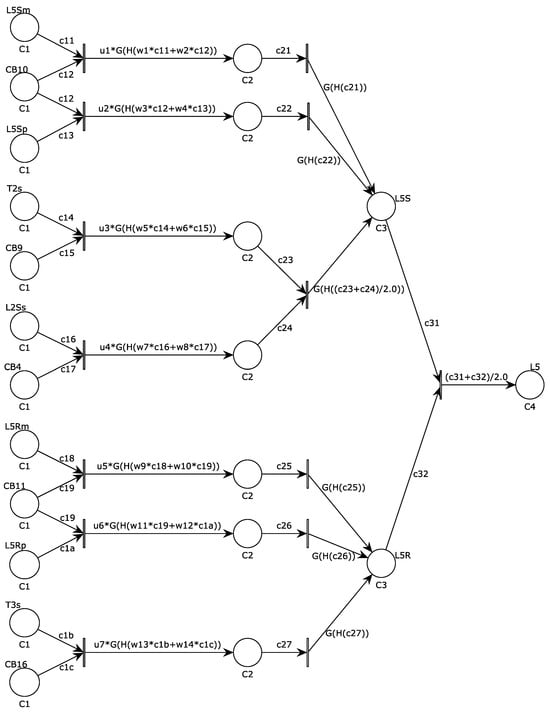
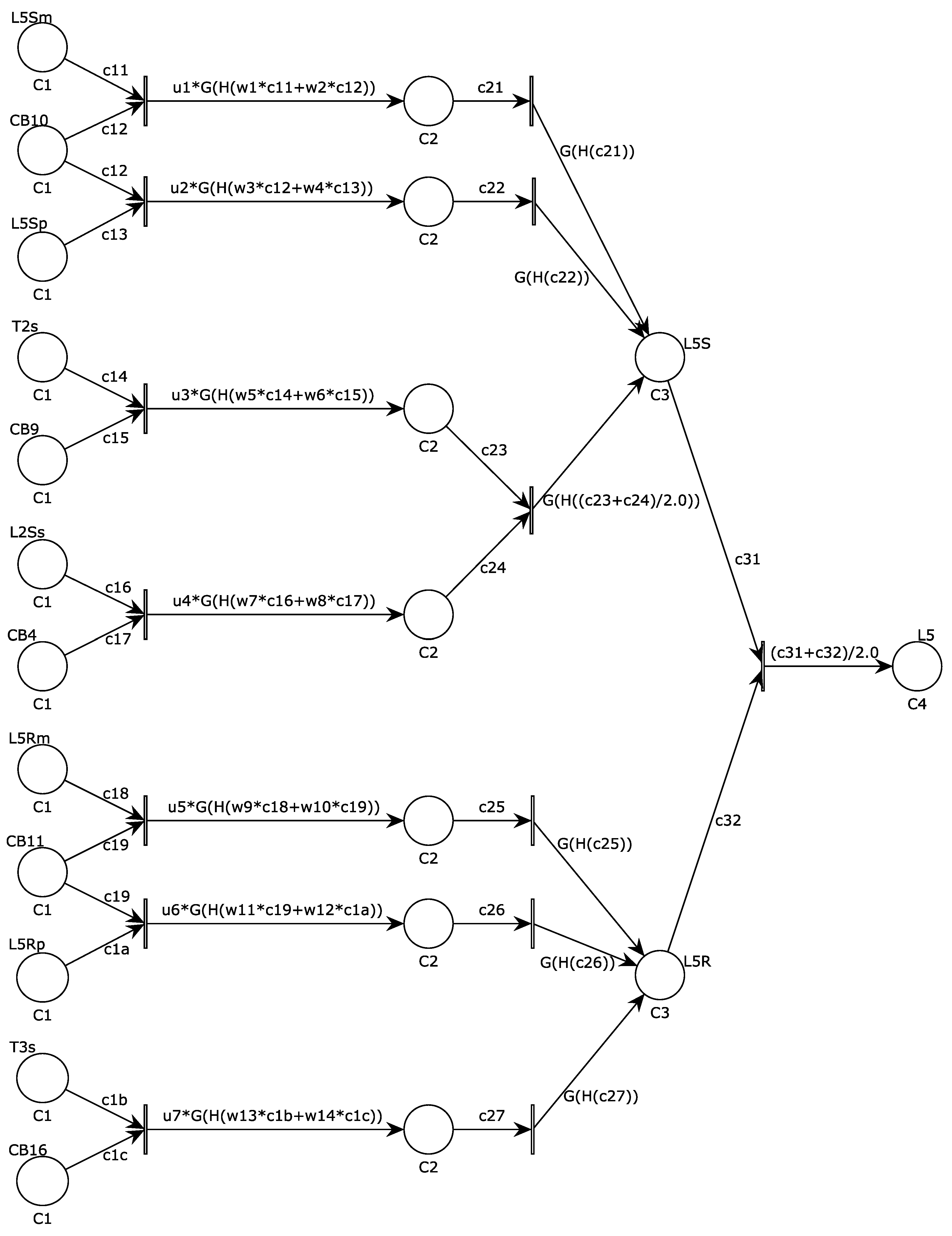
The FCPN inference module is constructed based on transforming hierarchical FPN models [12,14] into an equivalent structure. Taking A3 and L5 in Figure 3 as examples, their respective inference modules are shown in Figure 6 and Figure 7. The module treats confidence as a monochromatic token, providing the prerequisite for synthesizing alarm information to evaluate initial confidence and establish an integrated FCPN diagnostic model.

Figure 6. FCPN inference module for A3.

Figure 7. FCPN inference module for L5.

In Figure 6 and Figure 7, S and R denote the sending end (left, upper side) and receiving end (right, lower side) of the line, respectively. The superscripts m, p, and s respectively represent main protection, near backup protection, and far backup protection.

For instance: A3m indicates the main protection for bus A3; L5Sp denotes the near backup protection for the sending end of line L5; T3s signifies the far backup protection for transformer T3.

Aligned with the reasoning mechanism of hierarchical FPN, the FCPN inference module executes backward reasoning along the propagation direction of component faults. Within the module, the first layer place from the left represents the proposition “a protection or circuit breaker has tripped”; the second layer place indicates “confirmation that a protection and its corresponding circuit breaker have tripped”; the third layer place denotes a specific propagation direction of a component fault; and the fourth layer place is the termination place, signifying “a component has failed”. Color sets $C1$, $C2$, $C3$, and $C4$ respectively define the confidence tokens stored in each layer’s places.

The parameters for the inference module, including weights, thresholds, and output functions, are configured following the principles established in [12,14], with specific adaptations for the FCPN structure.

For the first-layer input weights $w_1,w_2,\dots ,w_n$, corresponding to whether the place represents protection or circuit breaker, they are set to 0.54 and 0.46, respectively. For input weights in the second and third layers, if the corresponding transition has multiple input places, the input weight is set to the reciprocal of the number of places, ensuring the output confidence is the average of the corresponding proposition confidences; otherwise, the input weight is set to 1.

The first-layer output weights $u_1,u_2,\dots ,u_m$ are set to 1, 0.95, and 0.85 corresponding to main protection, near backup protection, or far backup protection, respectively. For other layers, the output weight is set to 1.

The transition threshold for both the first and second layers is set to 0.2, while no threshold is set for the third layer transition.

The output confidence for the first and second layers is corrected by a Gaussian function, defined as:

$$G\left(x\right)=e^{-\alpha {(x-1)}^2}$$

(2)

where x represents the output confidence Based on [14], conduct the operation for determining the value of $\alpha$. Setting $\alpha =3$ ensures that when $x<0.5$, a lower output confidence is obtained to suppress false diagnosis; conversely, when $x\ge 0.5$, a higher output confidence is achieved to reinforce correct diagnosis.

4.2. Initial Confidence Assessment Module

In existing FPN methods, the confidence of a tripped protection or circuit breaker is typically determined by its correct operation rate over a past period. This prior probability assignment approach fails to adequately consider specific fault alarm information. When protection devices experience failure to operate or misoperation, or when alarm information suffers from underreporting or misreporting, it may lead to misjudgments or misclassifications of faulty components [17]. To overcome this limitation, this work introduces a dedicated initial confidence assessment module. This module dynamically evaluates the initial confidence for each alarm by synthesizing multiple information streams: the operational state of the device, its self-check alarm status, and the precise timing of the action. This context-aware assessment provides a more robust and accurate input for the subsequent inference module.

4.2.1. Assessment of Operation State Confidence

Modern protection devices are equipped with self-diagnostic functions that typically generate a self-check warning when internal anomalies are detected, which may coincide with false alarms or missed alarms in the operation information. Crucially, however, a self-check warning is not a definitive indicator of an incorrect operation report. Modern protection devices are equipped with self-diagnostic functions that typically generate a self-check warning when internal anomalies are detected, which may coincide with false alarms or missed alarms in the operation information [8]. The proposed method evaluates the confidence of operation status based on self-check information received by the dispatch center regarding the operation of protection or circuit breakers. The mapping rules for this assessment, derived from system reliability considerations and expert knowledge, are summarized in Table 4.

Table 4. Mapping for operation state confidence assessment.

Protection Devices	No Self-Check Alarm		Self-Check Alarm
	No Operation	Operation	No Operation	Operation
Main Protection	0.1	0.95	0.4	0
Near-Backup Protection	0.1	0.9	0.4	0
Far-Backup Protection	0.1	0.85	0.4	0
Circuit Breaker	0.1	0.85	0.4	0

The confidence values in Table 4 are derived from three sources. First, the base values for the “Operation, No Self-Check Alarm” column are anchored to the minimum correct operation rates specified in Chinese relay protection standards (GB/T 14285, DL/T 995): main protection 0.95, near-backup 0.90, far-backup 0.85, and circuit breaker 0.85. Second, the effect of a self-check alarm is modeled based on field reliability data [17]: a self-check alarm is treated as halving the confidence in a reported operation (mapping to 0 for operation-with-alarm), while raising the confidence in a missed operation to 0.4 to reflect the elevated probability of device malfunction. Third, all values were validated against the four case studies in Section 5; no adjustment beyond the standard-based initialization was required.

4.2.2. Assessment of Operating Timing Confidence

Following the methodologies in [12,14], this work utilizes time interval constraints for operations of protections and circuit breakers. By performing backward reasoning on the temporal information of operations received by the dispatch center, it derives time constraints for the cause events corresponding to faults. Subsequently, forward reasoning is applied to obtain time point constraints for operations, thereby validating the temporal information of operations and enabling assessment of the confidence of operational timing. Let T denote a time point, and let $D(T_i,T_j)$ denote the time interval from $T_i$ to $T_j$. The time interval constraints for operations of protections and circuit breakers are defined as follows:

$$D(T_v,T_m)=[10,40]\mathrm{ms}$$

(3)

$$D(T_v,T_p)=[260,340]\mathrm{ms}$$

(4)

$$D(T_v,T_s)=[950,1070]\mathrm{ms}$$

(5)

$$D(T_K,T_{\mathrm{CB}})=[20,40]\mathrm{ms}$$

(6)

$$D(T_v,T_{\mathrm{CB}})=D(T_v,T_K)+D(T_K,T_{\mathrm{CB}})$$

(7)

where v denotes the cause event, m, p, and s represent the main protection, near-backup protection, and far-backup protection, respectively. K represents various protections, namely m, p, or s. And CB denotes the circuit breaker.

Let the time point when the failure-causing event occurred be $t_v$. By performing backward reasoning on the temporal information $t_1,t_2,\dots ,t_n$ for operations of protections and circuit breakers, multiple time constraints $T_{v_1},T_{v_2},\dots ,T_{v_n}$ for potential cause events are derived. The intersection of these time constraints is taken to ultimately determine the time constraints $T_v^{\prime }$ for the cause event. The specific operations for backward reasoning are as follows:

$$T_{v_i}=t_i-D(t_v,t_i)$$

(8)

$$T_v^{-}=max\left(T_{v_1},T_{v_2},\dots ,T_{v_n}\right)$$

(9)

$$T_v^{+}=min\left(T_{v_1},T_{v_2},\dots ,T_{v_n}\right)$$

(10)

$$T_v^{\prime }=\left[T_v^{-},T_v^{+}\right]$$

(11)

where $i=1,2,\dots ,n$.

Through forward reasoning, the time point constraints $T_1^{\prime },T_2^{\prime },\dots ,T_n^{\prime }$ for the operation of each protection and circuit breaker are obtained, with the specific calculations as follows:

$$T_i^{\prime }=T_v^{\prime }+D(t_v,t_i)$$

(12)

where $i=1,2,\dots ,n$.

Verify the temporal information $t_1,t_2,\dots ,t_n$ of each protection and circuit breaker sequentially, determining whether $t_i\in T_i^{\prime }$, where $i=1,2,\dots ,n$. If $t_i\in T_i^{\prime }$, the corresponding protection device or circuit breaker’s operating timing confidence is 1; if $t_i\notin T_i^{\prime }$, the operating timing confidence is 0.

4.2.3. Comprehensive Assessment of Initial Confidence

For the operation of a certain protection or circuit breaker, let the state confidence be $C_s$ and the timing confidence be $C_t$. The initial confidence $C_i$ of the operation is obtained by synthesizing $C_s$ and $C_t$. The synthesis formula is as follows:

$$C_i=0.55C_s+0.45C_t$$

(13)

Considering that the operation time information of the protection and the circuit breaker only appears after the change of the operation state, it is analogous to the first layer input weights of the FCPN inference module, which take values based on whether the input place represents protection or the circuit breaker. Therefore, the weight values of $C_s$ and $C_t$ are set to 0.55 and 0.45, respectively.

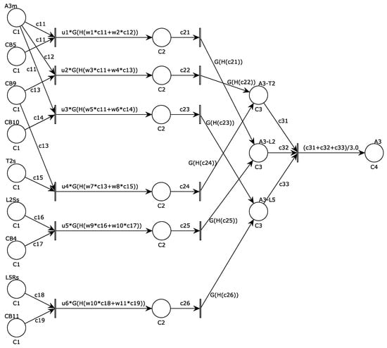
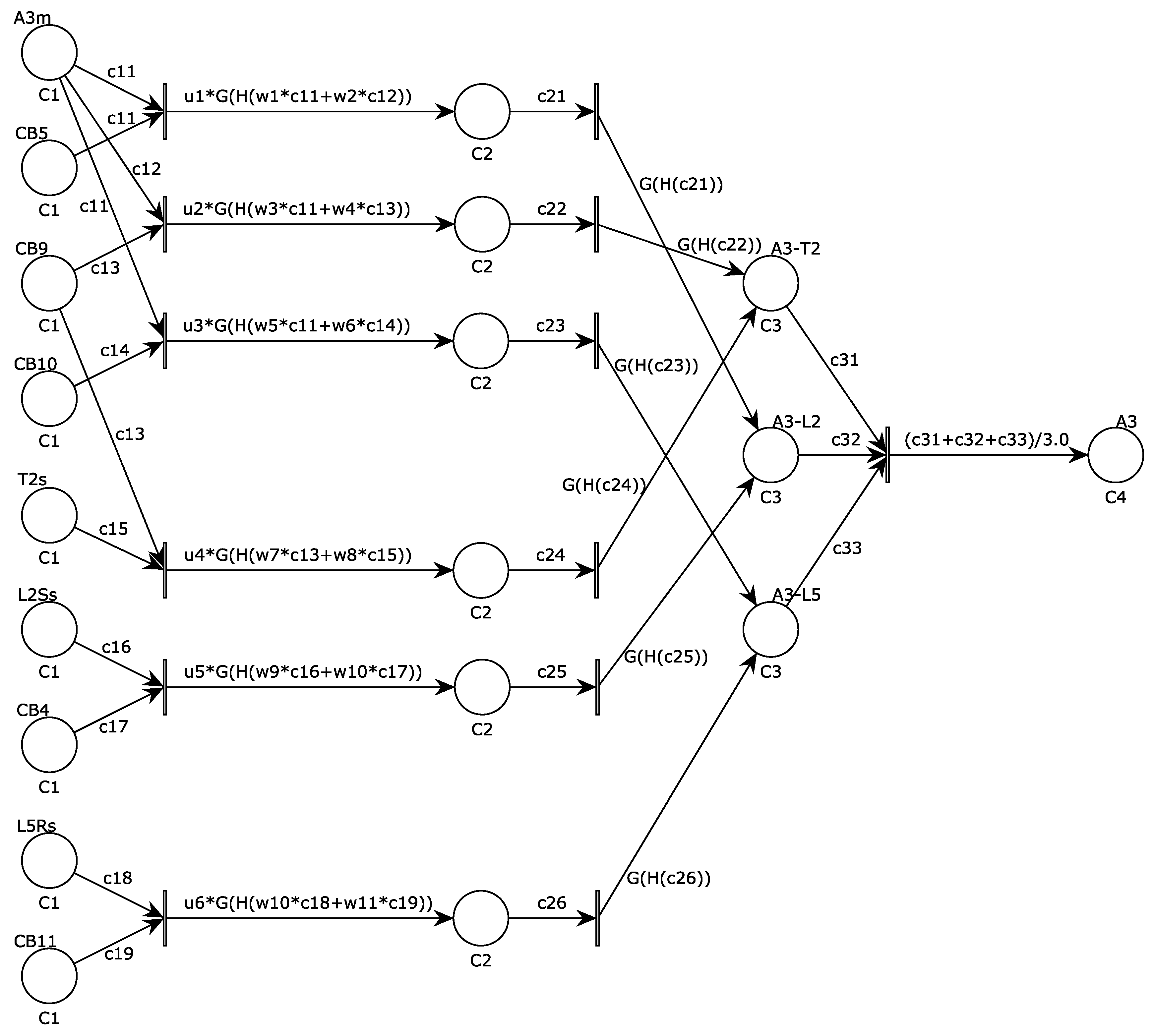
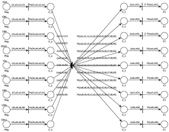
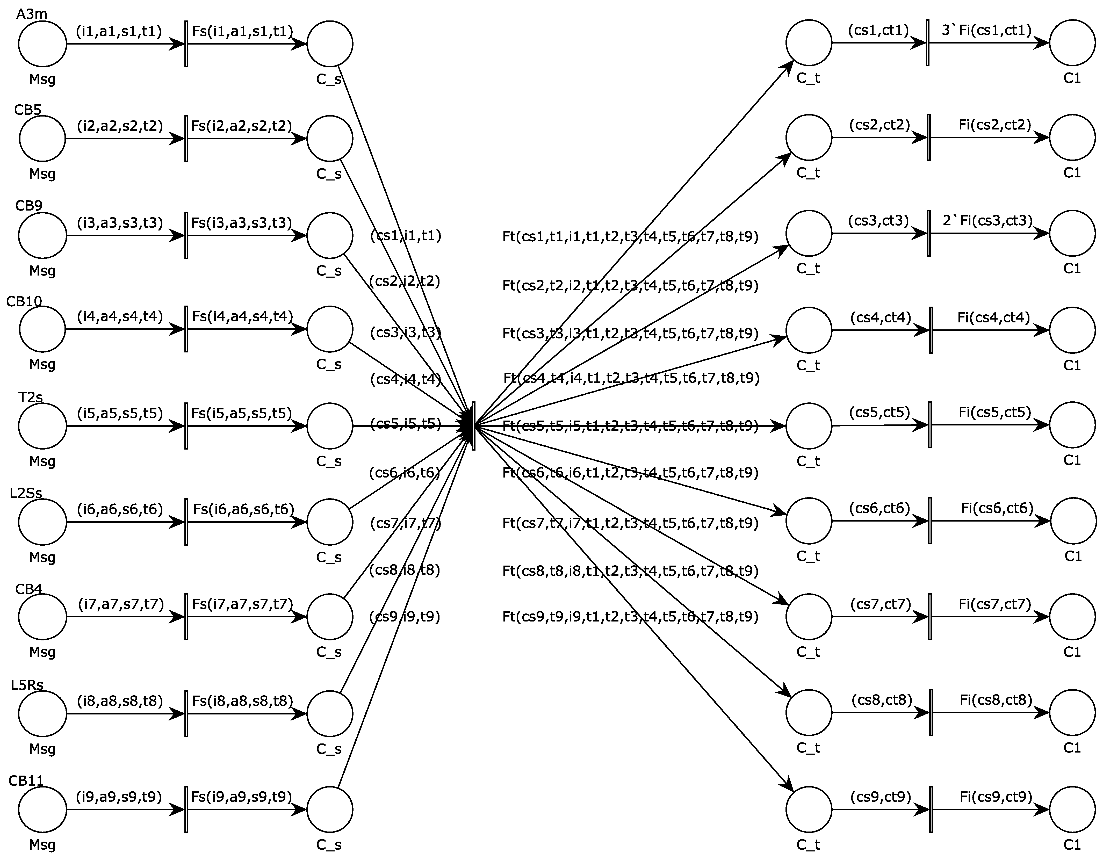
Based on the aforementioned principles, the initial confidence assessment module is established, taking A3 in Figure 3 as an example, as shown in Figure 8.

Figure 8. Initial confidence assessment module for A3.

The module’s color sets, token types and token attributes are introduced in Table 5 and Table 6, respectively.

Table 5. Color sets for the initial confidence assessment module.

Color Set Definition	Representation Content
RP = with m|p|s|mk|pk|sk	Relay protection type, where mk/pk/sk denotes the corresponding protection for circuit breakers m/p/s.
Msg = product RP*BOOL*BOOL*int	A tuple consisting of protection type, operation status, self-check status, and operation time.
C_s = product real*RP*int	A tuple consisting of operation state confidence, protection type, and operation time.
C_t = product real*real	A tuple consisting of operation state confidence and operation timing confidence.
C1 = real with 0.0..1.0	Initial confidence.

Table 6. Token types and attributes for the initial confidence assessment module.

Token Types and Attributes	Representation Content
(i,a,s,t):Msg	i indicates the corresponding protection for a specific protection or circuit breaker; a is a BOOL variable representing the operation state, where true/false indicates no operation/operation; s is a BOOL variable representing the self-check status, where true/false indicates no alarm/alarm; t denotes operation time.
(cs,i,t):C_s	$cs$ denotes operation state confidence, i, t as above.
(cs,ct):C_t	$ct$ denotes operation timing confidence, $cs$ as above.

The module undergoes three layers of transition, with corresponding output functions $Fs$, $Ft$, and $Fi$.

Function $Fs$ derives the corresponding operation state confidence from the operation and self-check information based on the mapping relationship in Table 4.

Function $Ft$ derives operation time point constraints using Equations (8)–(12), then calculates the corresponding operation timing confidences by verifying temporal information of operations.

Function $Fi$ determines the initial confidence for the operation of a specific protection or circuit breaker using Equation (13). The timing information is derived from the wide-area synchronization system of the power grid. Its reliability is relatively independent of the internal self-checking status of the protection device. Therefore, even if there is a self-check alarm, the timing information still retains some reference value. The weighted combination of the two can provide a more robust initial confidence estimation compared to a single information source.

By sequentially firing the three layers of transition, the module successively obtains operation state confidences, operation timing confidences, and the initial confidences of operation information.

For components such as busbars and lines in an active distribution network, an initial confidence assessment module and an inference module are constructed for each component. By connecting these two modules in series—initial confidence assessment module followed by inference module—an FCPN suspected faulty component diagnosis model can be established for each grid component separately. By sequentially executing the initial confidence assessment module and the inference module, the FCPN diagnosis model can achieve accurate diagnosis of the corresponding suspected faulty components.

Although the settings of weights, thresholds, and output functions in the inference module of the FCPN diagnosis model, as well as the assessment of operating timing confidence in the initial confidence assessment module, are based on [12,14], the FCPN diagnosis model reconstructs the reasoning logic of fault confidence. Refs. [12,14] require pre-calculation and analysis of the initial confidences of operations for protections and circuit breakers before invoking the FPN model, resulting in low diagnostic efficiency and poor process continuity. Moreover, the fault symptom information processed in [12,14] mainly includes operation information and temporal information of relay protection devices, with insufficient information richness that affects diagnostic accuracy.

Compared with similar methods, the FCPN diagnosis model proposed in this paper exhibits more prominent advantages in fault diagnosis for active distribution networks. It assigns colors to confidence tokens, enabling integrated and visual reasoning from multi-source fault symptom information to fault confidence. Specifically, the model first directly uses the self-check information and timing information of relay protection actions to evaluate the initial confidences of operations for protections and circuit breakers, and then obtains the fault confidences of suspected components through layer-by-layer confidence reasoning. These advantages not only overcome the defect in other similar methods where initial confidence relies only on prior probability assignment approach, but also significantly improve the diagnostic accuracy for suspected faulty components. Relevant case verification will be presented later.

5. Case Study and Comparison

5.1. Fault Diagnosis Process

Based on the foregoing introduction to the CPN fault zone search model and the FCPN suspected faulty component diagnosis model, this paper proposes a fault diagnosis process based on multi-source fault symptom information. When the dispatch center receives alarms from the active distribution network, the fault diagnosis process proceeds as follows:

• Update the CPN fault area search model based on circuit breaker operation information, then run the model to identify all suspected faulty components.
• Sequentially retrieve the FCPN diagnosis models for each suspected faulty component. By executing their respective initial confidence assessment modules and inference modules, obtain the corresponding fault confidence for each component.
• Given that the fault diagnosis accuracy of the method presented in this paper is relatively high, this paper adopts a higher final fault confidence threshold of 0.75 compared to similar methods. If the confidence of a suspected faulty component is greater than or equal to 0.75, it is deemed faulty; otherwise, it is considered in normal state.
• Based on the diagnosis results, evaluate the operations of protections and circuit breakers against the alarm information [12].

5.2. Case Verification

Taking the A3 fault in Figure 3 as an example, the dispatch center received alarm information (A3m, 12 ms), (CB5, 35 ms), (CB9, 37 ms), (L5Rs, 990 ms), (CB11, 1015 ms), and a self-check alarm indicating abnormal operation of CB10.

The specific fault diagnosis process is as follows:

• For tripped circuit breakers CB5, CB9, and CB11, update and run the CPN fault zone search model to identify suspected faulty components A3 and L5. Refer to Section 2.3 for the detailed process.
• The A3 diagnosis process is as follows:

  (a)

  Retrieve the FCPN diagnosis model for A3, and store the information of protections and circuit breakers as composite color tokens in the first-layer places of the initial confidence assessment module shown in Figure 8:

  $$\begin{array}{cc}\hfill {\mathit{P}}_1=& \left[\right(\mathrm{m},\mathrm{false},\mathrm{true},12),(\mathrm{mk},\mathrm{false},\mathrm{true},35),(\mathrm{mk},\mathrm{false},\mathrm{true},37),\hfill \\ & (\mathrm{mk},\mathrm{true},\mathrm{false},⌀),(\mathrm{s},\mathrm{true},\mathrm{true},⌀),(\mathrm{s},\mathrm{true},\mathrm{true},⌀),\hfill \\ & (\mathrm{sk},\mathrm{true},\mathrm{true},⌀),(\mathrm{s},\mathrm{false},\mathrm{true},990),(\mathrm{sk},\mathrm{false},\mathrm{true},1015)];\hfill \end{array}$$

  (b)

  Fire the first-layer transitions of initial confidence assessment module to generate operation state confidences, which is stored in the second-layer places:

  $$\begin{array}{cc}\hfill {\mathit{P}}_2=& \left[\right(0.95,\mathrm{m},12),(0.85,\mathrm{mk},35),(0.85,\mathrm{mk},37),(0.4,\mathrm{mk},⌀),(0.1,\mathrm{s},⌀),\hfill \\ & (0.1,\mathrm{s},⌀),(0.1,\mathrm{sk},⌀),(0.85,\mathrm{s},990),(0.85,\mathrm{sk},1015)];\hfill \end{array}$$

  (c)

  Fire the second-layer transitions of initial confidence assessment module to generate operation timing confidences, which is stored in the third-layer places:

  $$\begin{array}{cc}\hfill {\mathit{P}}_3=& \left[\right(0.95,1),(0.85,1),(0.85,1),(0.4,0),(0.1,0),\hfill \\ & (0.1,0),(0.1,0),(0.85,1),(0.85,1)];\hfill \end{array}$$

  (d)

  Fire the third-layer transitions of initial confidence assessment module to generate initial confidences, which is stored in the fourth-layer places:

  $$\begin{array}{cc}\hfill {\mathit{P}}_4=& [3^{\prime }0.9725,0.9175,2^{\prime }0.9175,0.4,0.1,0.1,0.1,0.9175,0.9175];\hfill \end{array}$$

  (e)

  The initial confidences stored in the fourth-layer places of this module are passed to the first-layer places of the inference module, The confidences of the first-layer places in the inference module are then:

  $$\begin{array}{cc}\hfill {\mathit{P}}_1^{\prime }=& [3^{\prime }0.9725,0.9175,2^{\prime }0.9175,0.4,0.1,0.1,0.1,0.9175,0.9175];\hfill \end{array}$$

  (f)

  Fire the first-layer transitions of the inference module to generate confidences of the second-layer places within that module:

  $${\mathit{P}}_2^{\prime }=[0.9917,0.9917,0.7759,0,0,0.8328];$$

  (g)

  Fire the second-layer transitions of the inference module to generate confidences of the third-layer places within that module:

  $${\mathit{P}}_3^{\prime }=[0.9998,0.9998,0.8601\&0.9196];$$

  (h)

  Fire the third-layer transition of the inference module; for each input confidence of this transition, take the maximum confidence value from the corresponding place, thereby the final termination place’s confidence is 0.9731.

• In summary, the fault confidence for A3 is 0.9731 > 0.75, indicating that A3 is the faulty component. Similarly, the fault confidence for L5 determined through diagnosis is 0.0738 < 0.75, indicating that L5 is not the faulty component.
• The final conclusion is that the fault occurred at busbar A3, and circuit breaker CB10 failed to operate.

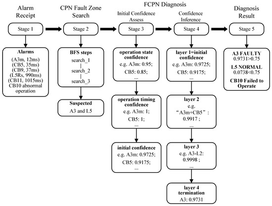
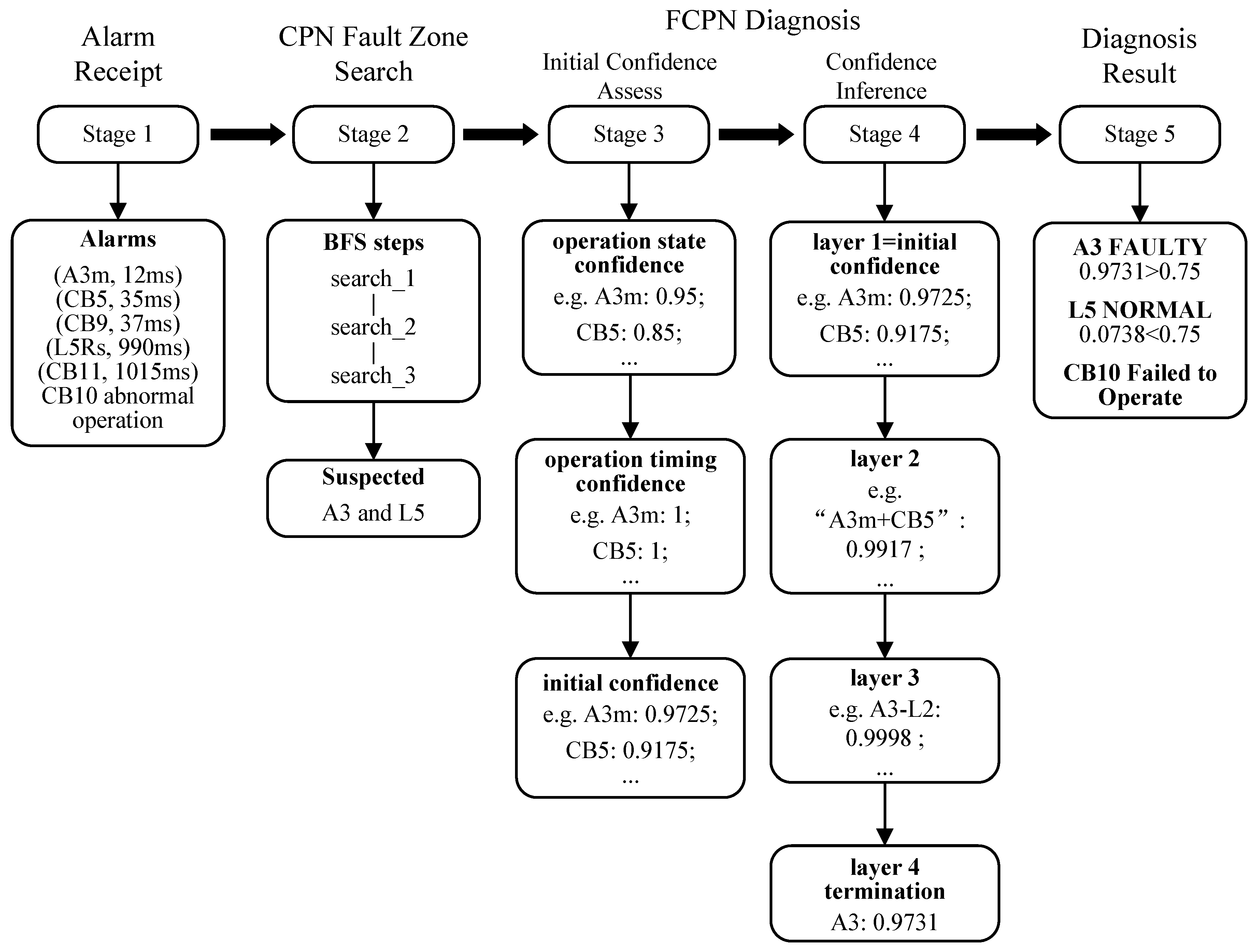
This section presents the complete step-by-step confidence evolution for case 1 (A3 fault scenario), covering both the faulty component A3 and the non-faulty suspected component L5. Figure 9 provides a unified visual representation of this process.

Figure 9. A flowchart combined with confidence values.

The diagnosis process adopted in the above case verification is general. When extended to other active distribution networks with conventional structures, it only needs to update the token values of relevant places in the CPN fault zone search model according to the network topology, and construct the corresponding FCPN diagnosis models for each power component based on the modeling method in Section 4 to complete the adaptation.

5.3. Comparison and Analysis

For the active distribution network depicted in Figure 3, this paper designs multiple potential fault scenarios, as shown in Table 7. Concurrently, the modeling and simulation of the proposed method and those from [14,15] are implemented on the CPN IDE platform, with diagnosis results compared as presented in Table 8.

Table 7. Possible fault scenarios in the active distribution network.

Case	Alarm Information
1	(A3m, 12 ms), (L5Rs, 990 ms), (CB5, 35 ms), (CB9, 37 ms), (CB11, 1015 ms), CB10 abnormal operation
2	(L9m, 5 ms), (L9p, 280 ms), (T3s, 960 ms), (CB10, 973 ms), (CB16, 985 ms), L5Ss abnormal alarm, CB15 abnormal operation
3	(L5Rm, 5 ms), (L5Sm, 10 ms), (L5Sp, 278 ms), (T2s, 977 ms), (L2Ss, 980 ms), (CB11, 26 ms), (CB5, 300 ms), (CB4, 1002 ms), (CB9, 1007 ms), CB5, CB10 abnormal operation
4	(L2Sm, 10 ms), (L2Rm, 15 ms), (L5Sm, 72 ms), (L5Rm, 75 ms), (A3m, 100 ms), (L2Rp, 284 ms), (L5Rp, 338 ms), (T3s, 1025 ms), (CB5, 39 ms), (CB10, 95 ms), (CB16, 1047 ms), A3m, CB4 abnormal alarm L2Rp, CB11 abnormal operation

Table 8. Comparison of fault diagnosis results between this method and other methods.

Case	This Paper Method			[14] Method		[15] Method		Actual Faulty Component
	Fault Zone	Confidence	Operation Evaluation	Confidence	Operation Evaluation	Confidence	Operation Evaluation
1	A3 L5	0.9731 0.0738	CB10 failed to operate	0.9194 0.3370	CB10 failed to operate	0.9770 0.0892	CB10 failed to operate	A3
2	L5 A6 L9	0.2218 0.4843 0.8601	L5Ss underreporting, CB15 failed to operate	0.4096 0.5424 0.7477	L5Ss underreporting, CB15 failed to operate	0.2661 0.7581 0.8700	L5Ss underreporting, CB15 failed to operate	L9
3	L2 A3 L5	0.1800 0.3065 0.9597	CB5 misoperation, CB10 failed to operate	0.1942 0.5258 0.8792	CB5 misoperation, CB10 failed to operate	0.2661 0.3171 0.9665	CB5 misoperation, CB10 failed to operate	L5
4	L2 A3 L5 A6	0.9299 0.1002 0.9597 0.1944	A3m misreporting, L2Rp misoperation, CB4 underreporting, CB11 failed to operate	0.3563 0.7530 0.4096	L2Sm misoperation, L2Rm misoperation, A3m misreporting, L2Rp misoperation, CB4 underreporting, CB11 failed to operate	0.1793 0.9665 0.2581	L2Sm misoperation, L2Rm misoperation, A3m misreporting, L2Rp misoperation, CB4 underreporting, CB11 failed to operate	L2 L5

Table 8 is structured as follows. Each case block (cases 1–4) lists the suspected faulty components identified by the CPN fault zone search (Fault Zone column) along with the fault confidence assigned to each component by each method (Confidence column) and the corresponding operation evaluation (Operation Evaluation column). A component is diagnosed as faulty if its confidence meets or exceeds the method’s threshold. The operation evaluation is derived post-diagnosis by comparing expected protection/breaker behavior against the received alarm set: absent expected alarms indicate failure-to-operate; present alarms inconsistent with the diagnosed fault location indicate misoperation or false alarm. As a worked example: in case 1, the proposed method assigns A3 a confidence of 0.9731 (≥0.75, diagnosed faulty) and L5 a confidence of 0.0738 (<0.75, diagnosed normal). The operation evaluation “CB10 failed to operate” follows from the observation that CB10—which should have tripped to isolate the A3 busbar fault—appears in the alarm list only with a self-check warning and no operation record, consistent with its low initial confidence of 0.4 in the assessment module. In Case 4, note that the Fault Zone for methods [14,15] contains only three components (L2 absent), indicating that the fault zone search stage of those methods failed to identify L2 as a suspected component—a limitation that the CPN self-check integration of the proposed method overcomes.

The final fault confidence thresholds for the proposed method and methods [14,15] are 0.75, 0.65, and 0.65, respectively. In Table 7 and Table 8, case 1 depicts a simple bus fault scenario, which all three methods accurately diagnose. Case 3 involves a line fault with dual-side protection where circuit breaker failure to trip and misoperation occur; all three methods also yield satisfactory diagnosis results. Case 2 involves a line fault with single-side protection, where protection underreporting and circuit breaker failure to trip occur; the methods proposed in this paper and in [14] both obtain accurate diagnosis results, whereas the method from [15] misdiagnoses bus A6 as faulty during diagnosis, primarily due to the excessively high initial confidence set by the circuit breaker place in its model design. Case 4 depicts a complex multiple-fault scenario: due to underreporting of alarm information from circuit breaker CB4, methods from [14,15] incorrectly define the fault zone and fail to include L2 among the suspected faulty components, ultimately leading to the misdiagnosis of L2’s failure; in contrast, this paper incorporates CB4 as a boundary circuit breaker into the CPN fault zone search model based on self-check information, thereby identifying all suspected faulty components.

In the aforementioned fault scenarios, this paper achieves accurate diagnosis results even when protection or circuit breakers fail to operate, misoperation, or when alarm information suffers from underreporting, misreporting. Although the confidences of the faulty components identified by this paper is slightly lower than that of the method in [15], this paper avoids misjudgments or omissions of power grid components, resulting in more accurate and comprehensive diagnosis results. Simultaneously, the confidences of non-faulty components diagnosed by this method are significantly lower than that in [14,15], enhancing the robustness of diagnosis results. The above analysis demonstrates that the fault diagnosis method proposed in this paper has higher fault tolerance and accuracy compared with similar methods in recent years.

6. Conclusions

This paper has proposed a two-stage fault diagnosis method for active distribution networks based on colored Petri nets and fuzzy colored Petri nets. A fault zone search model for colored Petri nets is developed using breadth-first search, identifying suspected faulty components based on circuit breaker operation information and grid topology. The model’s universality is validated through simulation examples. Building upon hierarchical fuzzy Petri nets, a diagnosis model using fuzzy colored Petri nets is constructed by assigning colors to confidence tokens. Initial confidence is first dynamically assessed by synthesizing self-check alarm data and operational timing information from protection devices and circuit breakers. Subsequently, the fault confidence for a suspected component is derived through hierarchical confidence inference. By integrating self-check and timing information from protection and circuit breaker operations, this paper introduces a more rational and context-aware initial confidence assessment method, addressing the fundamental shortcoming of static, experience-based assignment in existing approaches. Finally, through multiple simulation case studies and comparative analysis against state-of-the-art methods, the proposed approach is demonstrated to achieve rapid and accurate fault diagnosis in active distribution networks with high fault tolerance, offering significant practical value for real-world power system operation.

References

- Liu, L.; Zhai, R.; Hu, Y. Performance evaluation of wind-solar-hydrogen system for renewable energy generation and green hydrogen generation and storage: Energy, exergy, economic, and enviroeconomic. Energy 2023, 276, 127386. [Google Scholar] [CrossRef] [Scilit]
- Peng, X.; Liu, Z.; Jiang, D. A review of multiphase energy conversion in wind power generation. Renew. Sustain. Energy Rev. 2021, 147, 111172. [Google Scholar] [CrossRef] [Scilit]
- Zhou, X.; Xue, S.; Du, H.; Ma, Z. Optimization of building demand flexibility using reinforcement learning and rule-based expert systems. Appl. Energy 2023, 350, 121792. [Google Scholar] [CrossRef] [Scilit]
- Thomas, J.B.; Chaudhari, S.G.; Shihabudheen, K.V.; Verma, N.K. CNN-Based Transformer Model for Fault Detection in Power System Networks. IEEE Trans. Instrum. Meas. 2023, 72, 2504210. [Google Scholar] [CrossRef] [Scilit]
- Siddique, M.N.I.; Shafiullah, M.; Mekhilef, S.; Pota, H.; Abido, M.A. Fault classification and location of a PMU-equipped active distribution network using deep convolution neural network (CNN). Electr. Power Syst. Res. 2024, 229, 110178. [Google Scholar] [CrossRef] [Scilit]
- Khadse, C.; Patharkar, A.A.; Chaudhari, B.S. Electromagnetic field and artificial intelligence based fault detection and classification system for the transmission lines in smart grid. Energy Sources Part A-Recovery Util. Environ. Eff. 2021, 7, 1948637. [Google Scholar]
- Zhang, X.; Ding, R.; Wang, Z.; Guo, Z.; Liu, B.; Wei, J. Power grid fault diagnosis model based on the time series density distribution of warning information. Int. J. Electr. Power Energy Syst. 2023, 146, 108774. [Google Scholar] [CrossRef] [Scilit]
- Dong, M.; Zhang, Y.; Zhang, Y.; Wen, F.; Sun, W.; Wang, C. An analytic model for power system fault diagnosis employing electrical data. Autom. Electr. Power Syst. 2023, 37, 55–62. [Google Scholar]
- Calderaro, V.; Hadjicostis, C.N.; Piccolo, A.; Siano, P. Failure Identification in Smart Grids Based on Petri Net Modeling. IEEE Trans. Ind. Electron. 2011, 58, 4613–4623. [Google Scholar] [CrossRef] [Scilit]
- Jiang, Z.; Li, Z.; Wu, N.; Zhou, M. A Petri Net Approach to Fault Diagnosis and Restoration for Power Transmission Systems to Avoid the Output Interruption of Substations. IEEE Syst. J. 2018, 12, 2566–2576. [Google Scholar] [CrossRef] [Scilit]
- Yang, J.; He, Z.; Zang, T. Power system fault-diagnosis method based on directional weighted fuzzy Petri nets. Proc. Chin. Soc. Electr. Eng. 2010, 30, 42–49. [Google Scholar]
- Xu, B.; Yin, X.; Yin, X.; Wang, Y.; Pang, S. Fault Diagnosis of Power Systems Based on Temporal Constrained Fuzzy Petri Nets. IEEE Access 2019, 7, 101895–101904. [Google Scholar] [CrossRef] [Scilit]
- Zhang, X.; Yue, S.; Zha, X. Method of power grid fault diagnosis using intuitionistic fuzzy Petri nets. IET Gener. Transm. Distrib. 2018, 12, 295–302. [Google Scholar] [CrossRef] [Scilit]
- Yang, F.; Yu, Y. Fault diagnosis of distribution network based on time constrained hierarchical fuzzy Petri nets. Power Syst. Prot. Control 2020, 48, 99–106. [Google Scholar]
- Cheng, X.; Zhuang, X.; Meng, L. Fault Diagnosis Method of Power Grid Based on Weighted Fuzzy Temporal Constraint Petri Net. Smart Power 2023, 48, 83–90. [Google Scholar]
- Chen, Q.; Zhou, X.; Sun, M.; Zhang, X. Fault Tracking Method for Relay Protection Devices. Energies 2021, 14, 2723. [Google Scholar] [CrossRef] [Scilit]
- Ying, L.; Jia, Y.; Li, W. Research on state evaluation and risk assessment for relay protection system based on machine learning algorithm. IET Gener. Transm. Distrib. 2020, 14, 3619–3629. [Google Scholar] [CrossRef] [Scilit]
- Jin, L.; Chen, Q.; Ji, J.; Zhou, X. A Power Grid Fault Diagnosis Method in the Case of Alarm Information Loss Based on the Top-k Skyline Query Algorithm. Energies 2021, 14, 6223. [Google Scholar] [CrossRef] [Scilit]
- Kaid, H.; Al-Ahmari, A.; N. Alqahtani, K. Fault Detection, Diagnostics, and Treatment in Automated Manufacturing Systems Using Internet of Things and Colored Petri Nets. Machines 2023, 11, 173. [Google Scholar] [CrossRef] [Scilit]
- The CPN-IDE Application. Available online: http://cpntools.org/cpn-ide (accessed on 23 April 2026).
- Jensen, K.; Kristensen, L.M. Coloured Petri Nets Modeling and Validation of Concurrent Systems, 1st ed.; Springer: Berlin, Germany, 2009; pp. 83–87. [Google Scholar]
- Cheng, M.; Zhang, X.; Xu, M.; Xue, Y.; Wu, W.; He, Y. Location method of an active distribution network fault section based on multi—Target weighted grey target decision. Power Syst. Prot. Control 2021, 49, 124–132. [Google Scholar]
- Sevov, L.; Khan, U.; Zhang, Z. Enhancing Power Transformer Differential Protection to Improve Security and Dependability. IEEE Trans. Ind. Appl. 2017, 53, 2642–2649. [Google Scholar] [CrossRef] [Scilit]
- Kaur, K.; Rana, R.; Kumar, N.; Singh, M.; Mishra, S. A colored petri net based frequency support scheme using fleet of electric vehicles in smart grid environment. IEEE Trans. Power Syst. 2016, 31, 4638–4649. [Google Scholar] [CrossRef] [Scilit]
Disclaimer/Publisher’s Note: The statements, opinions and data contained in all publications are solely those of the individual author(s) and contributor(s) and not of MDPI and/or the editor(s). MDPI and/or the editor(s) disclaim responsibility for any injury to people or property resulting from any ideas, methods, instructions or products referred to in the content. |
© 2026 by the authors. Licensee MDPI, Basel, Switzerland. This article is an open access article distributed under the terms and conditions of the Creative Commons Attribution (CC BY) license.