Short-Term Disaggregated Load Forecasting Using a Hybrid Fuzzy ARTMAP and K-means Clustering Model

Abstract

Accurate short-term load forecasting at disaggregated levels is critical for energy management in microgrids and institutional environments, yet it remains a challenge due to high consumption variability and limited contextual information. This paper proposes a hybrid model that combines Fuzzy ARTMAP neural networks with K-means clustering to improve hourly load forecasting using real data from a university microgrid. The methodology includes key preprocessing steps such as filtering low-load records, removing holidays, interpolating missing values, and applying cyclic encoding to standardize the data into 96 time intervals per day (15-min resolution). For each prediction, the average load profile of the five most recent weekdays is computed and compared to cluster centroids to identify the most similar group, which is then used to train the neural network. Results demonstrate consistent improvements in MAPE, RMSE, and MAE compared to the non-clustered baseline. The model showed robustness to non-stationary behavior and atypical patterns, even when relying solely on timestamp and load data. The proposed strategy outperformed conventional approaches and proved suitable for complex, data-limited environments.

1. Introduction

Short-term electricity demand forecasting is an essential activity for the planning, operation, and efficient management of power systems. With the advancement of measurement technologies and the increasing variability of consumption patterns, especially in low-aggregation environments, the challenges associated with modeling and estimating electrical load have become more complex and uncertain [1]. These challenges are intensified by the nonlinear dynamics of load profiles and their sensitivity to exogenous factors, such as weather conditions and user behavior [2,3].

Disaggregated systems, such as microgrids or institutional environments, present significant consumption variations due to irregular occupancy, intermittent equipment operation, and the influence of academic or administrative calendars [4]. Such characteristics reduce the predictability of load profiles and limit the smoothing effect typical of more aggregated systems [5]. Therefore, it is necessary to adopt models capable of handling noisy data, abrupt changes, and irregular seasonal behaviors.

Among the methods applied to short-term load forecasting in low-aggregation environments, Artificial Neural Networks (ANNs) stand out due to their effectiveness in forecasting nonlinear time series, especially in this context. To improve their performance, these networks can be combined with clustering techniques, such as the K-means algorithm, which allows for their specialization on subsets of days with similar consumption patterns, increasing forecasting performance [5].

Building on this idea of segmentation, prior clustering has also been explored in a three-stage architecture composed of self-organizing maps, K-means clustering, and a multilayer perceptron ANN. This model was successfully validated for short-term forecasting in institutional microgrids. The model demonstrated the ability to adapt to operational variations and seasonal patterns characteristic of intermittently used environments [4].

Another approach with lower computational complexity is the Pattern Sequence-based Forecasting (PSF) method. This technique also performs initial clustering of load profiles using K-means and identifies historical consumption sequences similar to the target day’s pattern. Future load is then estimated based on the average of the subsequent loads, making it suitable for environments with cyclical and recurring behavior [6].

To improve data segmentation beyond traditional methods, the use of simulated annealing as a deterministic clustering technique has also been proposed, applied prior to neural network training. This strategy proved effective in separating heterogeneous load patterns, allowing greater model adherence to consumption profile characteristics [7].

In a different direction, other neural network architectures have been explored for this task. The application of Radial Basis Function Neural Networks in systems with high variability, such as real-time energy markets, has shown good performance in generalizing noisy and complex time series, reinforcing the viability of alternative architectures in challenging operational scenarios [8].

Despite these advances, a critical gap remains: many models are validated under idealized conditions that do not reflect real-world operational constraints. First, they often rely on ex-post data from the forecast day itself, a condition that is unfeasible in practical ex-ante forecasting scenarios where only past information is available [9]. Second, they frequently struggle with the operational irregularities of institutional settings—such as strikes, holidays, and academic calendar variations—which disrupt conventional time-series patterns and challenge model generalization.

This paper proposes a hybrid approach for hourly load forecasting at a disaggregated level. The methodology integrates Fuzzy ARTMAP neural networks with the K-means clustering technique, and is validated with real consumption data from a Brazilian public university. The proposed model was designed to estimate the demand for any day present in the database, considering only the hourly order of daily measurements, without requiring continuity between consecutive days.

The choice of the K-means algorithm aims to handle the high variability of consumption data. Instead of trying to teach a neural network to predict a consumption profile for a generic day, days with similar load profiles are grouped. This segmentation creates more homogeneous data subsets, which reduces noise and the complexity of the task for the neural network, resulting in more efficient training and specialized models for each type of consumption profile.

The selection of Fuzzy ARTMAP as the neural network for forecasting is also strategic. Unlike other architectures, this network is an incremental learning model, making it capable of learning new patterns without suffering from catastrophic forgetting [10]. Moreover, its Fuzzy component makes it resistant to outliers, allowing the model to generalize well even with imprecise data or unexpected peaks. The combination of these two techniques allows the approach to segment complexity (K-means) before applying a robust and adaptable model (Fuzzy ARTMAP).

The main novelty of this work lies in a framework that integrates clustering with incremental learning to improve forecasting in variable and non-stationary environments. While traditional models struggle to generalize from a single heterogeneous dataset, the proposed structure enhances forecast quality by allowing specialized networks to learn from stable, homogeneous patterns. This approach maintains the ability to update incrementally with new data—an intrinsic feature of Fuzzy ARTMAP—and ensures scalability for continuous data streams. It thus provides a practical solution for common forecasting challenges, including limited historical data, unmeasured variables, and high variability in user behavior.

The effectiveness of the proposed methodology, with and without the clustering step, is compared. For a more comprehensive validation, the approach’s performance will be benchmarked against other forecasting algorithms, including Multilayer Perceptron (MLP) and Decision Trees. This comparative analysis highlights the advantages of the hybrid approach for the unique challenges of disaggregated load forecasting in institutional environments.

2. Materials and Methods

This section details the data used and the methodological procedures for the construction, training, and validation of the proposed forecasting model.

2.1. Data Description

This study utilizes a real-world dataset of active energy measurements from a single building block at a Brazilian university. Data were collected from instruments connected directly to the building’s exclusive transformer, ensuring a truly disaggregated load profile free from the influence of external consumption sources.

Measurements were taken continuously from 24 April 2012 to 22 August 2013. The dataset features high temporal granularity, originally distributed in intervals close to 15 min, although with slight variations in time stamps, which were subsequently regularized during the preprocessing stage.

The analyzed period includes atypical operational events, such as an academic strike, holidays, and low-occupancy phases, resulting in irregular consumption patterns and abrupt variations. The time series also presents noise and anomalous values, attributed to acquisition failures or actual disturbances in the electrical system. These characteristics create a challenging yet ideal test case for evaluating the robustness of forecasting models in non-stationary environments.

2.2. Data Preprocessing

The data preprocessing stage was designed to standardize the time series and filter out non-representative operational patterns. The process involved regularizing time records, cyclically encoding the time variable, excluding non-representative observations, and filling in missing data.

Although the raw data had a nominal 15-min granularity, variations in timestamps were observed due to imperfections in the acquisition system. Therefore, the data was temporally regularized, aligning load values to a strict 15-min grid. This step is important because models like Fuzzy ARTMAP rely on pattern similarity; irregular measurement intervals could lead to poor clusters. Regularization eliminated this bias, ensuring that daily consumption profiles were compared at equivalent time points. This preserved signal quality and allowed the network to be trained with more reliable data.

To preserve the cyclic nature of the time variable, trigonometric encoding was used. The total number of minutes from 00:00 was calculated for each record, and Equations (1) and (2) were applied to encode the time variable:

$${\mathrm{Hour}\_\mathrm{sine}}_i=sin\left({\displaystyle \frac{2\pi ·{\mathrm{Minutes}}_i}{1440}}\right)$$

(1)

$${\mathrm{Hour}\_\mathrm{cosine}}_i=cos\left({\displaystyle \frac{2\pi ·{\mathrm{Minutes}}_i}{1440}}\right)$$

(2)

After adjusting the time series to regular 15-min intervals, each full day contained 96 load records. Based on this standardization, all incomplete days were removed. Additionally, samples corresponding to national and municipal holidays, as well as days with total consumption below 5000 Wh, were excluded. This deliberate filtering focuses the model on representative operational patterns, preventing the noise from atypical days (such as holidays or periods of minimal activity) from degrading its forecasting performance on typical working days. In total, these filtering steps resulted in the removal of 138 days from the original dataset.

To fill occasional gaps, simple linear interpolation was used. The estimate for each missing value was obtained by the arithmetic mean of the two valid records immediately before and after the missing point. This technique is effective in preserving the local continuity of the series without introducing artificial oscillations.

2.3. K-Means Clustering

High variability in load profiles from disaggregated environments, such as institutional buildings, presents a challenge for forecasting models, especially in hourly forecasting contexts at a disaggregated level and with a limited set of input variables. The absence of complementary information—such as temperature, occupancy, or operational context—combined with the exclusive availability of date, time, and load, increases the complexity of the problem and demands additional segmentation strategies.

In this scenario, unsupervised clustering algorithms have proven effective in organizing highly variable load time series, allowing for the reduction of internal heterogeneity and the specialization of predictive models in more homogeneous subsets [4,5]. K-means was chosen due to its simplicity and its successful application in systems with high variability.

According to Hernández et al. [4], K-means can be incorporated into hybrid architectures based on neural networks and self-organizing maps, segmenting daily profiles with similar behaviors in institutional microgrids. This approach demonstrated significant gains in terms of accuracy and adaptation to seasonal and intermittent patterns, being particularly relevant for applications in educational environments.

Similarly, Panapakidis [5] argues that the prior grouping of daily profiles by similarity favors the construction of specialized models for different types of days, contributing to improved hourly forecasting in systems with high operational variability.

From a technical standpoint, the algorithm performs partitioning based on the minimization of Euclidean distance between input vectors and centroids, iteratively adjusting the groupings until convergence is reached. Each centroid represents an average behavior pattern of the group, which favors the structuring of data into more cohesive and interpretable sets [4].

In this study, K-means was used to group daily load profiles by analyzing each day’s consumption vector (the 96 15-min data points). Since K-means is sensitive to data scale, each weekday subset (e.g., all Mondays) was standardized using the Z-score before being processed by the algorithm. The mean and standard deviation parameters were calculated from the data used for model training.

For the technical implementation, the K-means++ initialization method was used to select initial centroids, as it promotes a more efficient and stable convergence by choosing initial points that are far from each other. The algorithm used the Euclidean distance metric, which is particularly suitable for time series data represented as vectors.

The number of clusters was fixed at three ($k=3$). While internal evaluation metrics like the Elbow Method are often used to find a statistically optimal number of clusters, such an approach was not aligned with the primary objective here. The main goal was to create operationally meaningful groups based on similar load behaviors, ensuring each subset had a sufficient number of days for effective model training. Therefore, this fixed value was a pragmatic choice to guarantee that each specialized Fuzzy ARTMAP network could be trained on a robust data sample, preventing the instability and poor generalization associated with sparse clusters.

This clustering step prepares the dataset for the Fuzzy ARTMAP network, allowing it to be trained with more homogeneous information. This approach maintains forecasting consistency even when daily data are unstable.

2.4. Proposed Hybrid Modeling for Load Forecasting

The forecasting strategy is based on a hybrid approach that integrates K-means clustering with the Fuzzy ARTMAP neural network. Fuzzy ARTMAP is a supervised learning model with incremental adaptation capabilities, composed of two Fuzzy ART modules, $AR{T}_a$ and $AR{T}_b$, which process the input and output vectors. These modules are interconnected by an inter-ART structure that manages the match tracking mechanism, ensuring learning stability. The network’s incremental learning feature eliminates the need to reprocess the entire historical dataset with each new input, which makes the architecture scalable and well-suited for environments with evolving load profiles [10,11,12]. (For a detailed description of the Fuzzy ARTMAP network’s architecture and learning mechanisms, see Appendix A).

The model was structured to operate with segmentation by weekday, from Monday to Friday. This approach aims to capture recurring consumption patterns while acknowledging that even within the same group, there is significant variability across days. This allows for a systematic evaluation of the predictor’s efficiency, considering the unique behavioral patterns of each daily profile. Weekends were excluded from the analysis due to their atypical and unrepresentative consumption profiles, as low campus occupancy on these days results in extremely low and irregular consumption.

To handle the high variability of load profiles and the absence of complementary information, such as temperature or occupancy data, the hybrid approach uses the output of K-means clustering (detailed in Section 2.3) to specialize the forecast. To predict a specific day, the average load curve of the five most recent weekdays ($l=5$) is calculated and compared to the obtained centroids; this value was chosen to provide a stable balance between capturing recent consumption trends and smoothing out single-day anomalies. Let $x_{d,t}$ be the load value on day d at time instant t. The average load at time t for these l days is given by Equation (3), and the complete average load curve vector is given by Equation (4):

$${\overline{x}}_t={\displaystyle \frac{1}{l}}\sum _{d=1}^l{x}_{d,t},t=1,2,\dots ,96$$

(3)

$$\overline{X}=\left({\overline{x}}_1,{\overline{x}}_2,\dots ,{\overline{x}}_{96}\right)$$

(4)

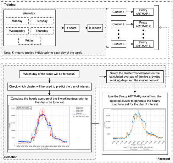
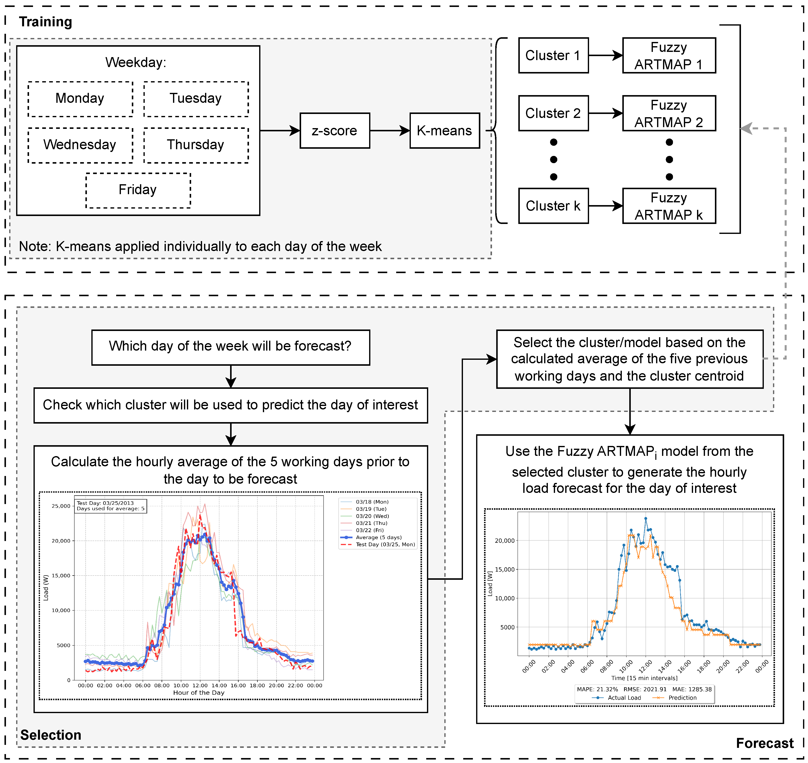
The overall methodology is summarized in the graphical representation presented in Figure 1. The complete pipeline can be broken down into two primary phases: an offline training phase and an online forecasting phase.

Figure 1. Graphical representation of the hybrid load forecasting methodology.

• Offline Training Phase (performed once for each weekday):
  • Data Segmentation: The historical dataset is first segregated by weekday (e.g., all Mondays).
  • Standardization: Each daily load profile within the subset is standardized using a Z-score.
  • Clustering: The K-means algorithm is applied to group the standardized profiles into k distinct clusters, each representing a typical consumption pattern.
  • Model Specialization: A separate Fuzzy ARTMAP network is trained exclusively on the data from each cluster, creating a pool of k specialized forecasting models.
• Online Forecasting Phase (performed for each target day):
  • Reference Curve Generation: A reference load curve is calculated by averaging the consumption profiles of the five most recent weekdays.
  • Cluster Selection: This reference curve is compared to the centroids of the k trained clusters, and the cluster with the highest similarity (i.e., minimum Euclidean distance) is selected.
  • Model Activation: The specialized Fuzzy ARTMAP model corresponding to the selected cluster is activated for the forecasting task.
  • Recursive Forecasting: The activated model generates the 24-h load forecast for the target day using the recursive mechanism.

The recursive mechanism mentioned above is a fundamental aspect of the model’s ex-ante design. It utilizes a sliding window of three time steps, $[x_{h-3},x_{h-2},x_{h-1}]$, to predict the load at step h. To generate the forecast for an entire day, the process begins by initializing the window with the last three known consumption values from the previous day. After the first prediction is made (e.g., for 00:00), the mechanism becomes fully recursive: this newly predicted value is fed back into the sliding window as an input to predict the next time step (e.g., 00:15). This iterative process continues for all 96 intervals of the day, ensuring the forecast is generated without any access to future consumption data. In addition to the load values, the network input at each step also includes the hour encoded using sine and cosine, as described in Section 2.2.

Formally, the recursive forecasting process can be expressed as follows:

$${\widehat{x}}_h=f(x_{h-3},x_{h-2},x_{h-1},{\mathrm{Hour}\_\mathrm{sine}}_h,{\mathrm{Hour}\_\mathrm{cosine}}_h),$$

(5)

where ${\widehat{x}}_h$ denotes the predicted load at time step h, and ${\mathrm{Hour}\_\mathrm{sine}}_h$ and ${\mathrm{Hour}\_\mathrm{cosine}}_h$ correspond to the trigonometric encodings of the time variable at that step.

2.5. Experimental Design and Evaluation

The effectiveness of the proposed approach was evaluated through a comparative analysis across three distinct modeling scenarios. (1) The proposed hybrid model, consisting of the complete K-means and Fuzzy ARTMAP architecture, was evaluated. (2) An ablation baseline was established to isolate the specific contribution of the clustering component. For this, a standalone Fuzzy ARTMAP network was trained without the initial clustering, using data from 15 randomly selected days of the same weekday as the target day, ensuring the day to be predicted was not in the training set. (3) A benchmark comparison was conducted to contextualize the model’s performance against two classic algorithms: a Multilayer Perceptron (MLP) and a Decision Tree. The MLP was chosen because it is a widely recognized benchmark and represents a different neural network paradigm from Fuzzy ARTMAP. The Decision Tree was selected as a representative of rule-based, non-parametric methods. This comparison against diverse, established models provides a more comprehensive validation of the proposed methodology.

The choice of using 15 days for training in the no-clustering scenario aims to simulate a practical setting with a limited historical data record while ensuring a sufficient sample volume for training. The Fuzzy ARTMAP network is particularly well-suited for this task. It can generalize patterns even with a small amount of data due to its incremental learning capability. This feature lets it learn new information without “forgetting” old patterns. By using random days, the approach forces the model to learn more general weekday patterns. It prevents the model from relying on short-term temporal dependencies. This is important because the network’s fuzzy component also makes it resistant to outliers and noise, allowing it to perform well even with imprecise or unexpected data points.

The overall validation process was conducted iteratively for all weekdays. For each weekday subset, the model was trained on all days but one, which was used for forecasting. This procedure was repeated until each day in the subset had been forecasted individually. This approach allows for the model’s performance to be evaluated in scenarios with limited historical series and without the requirement of temporal continuity between days.

To ensure optimal performance and prevent overfitting, the hyperparameters for all machine learning models—Fuzzy ARTMAP, MLP, and Decision Tree—were systematically tuned using a grid search methodology. Grid search is a technique that exhaustively searches a specified subset of the hyperparameter space for a model. It evaluates every possible combination of values from a predefined grid of parameters to identify the one that yields the best performance on a validation set [13]. This optimization was performed independently for each weekday subset (e.g., all Mondays) to ensure a fair comparison, where each model was fine-tuned for the specific data characteristics of that weekday. The set of parameters that yielded the lowest mean error on a validation set was then fixed and used for all subsequent forecasts within that specific weekday group. This approach ensures that the models generalize across the subset rather than specializing on individual days.

The parameter grids for each model were defined as follows:

• Fuzzy ARTMAP:
  • Input module vigilance parameter (${\rho }_a$): values between 0.90 and 0.99 with a step of 0.01;
  • Output module vigilance parameter (${\rho }_b$): values between 0.92 and 0.999 with a step of 0.001;
  • Inter-ART module vigilance parameter (${\rho }_{ab}$): fixed value of 0.8;
  • Learning rate ($\beta$): discrete values {0.1, 0.2, 0.5, 0.8, 1.0};
  • Choice parameter ($\alpha$): fixed value of 0.005.
• Multilayer Perceptron (MLP):
  • Hidden layer sizes: Varied architectures, including single layers (e.g., (5), (10), (20)) and multiple layers (e.g., (3, 8), (5, 25), (3, 5, 10)).
  • Activation function: relu and tanh.
  • Solver: Optimization algorithms Adam and L-BFGS.
  • Regularization term: 0.0001 and 0.001.
  • Learning rate schedule: constant and adaptive.
• Decision Tree:
  • Maximum depth: Unlimited, 5, 10, and 20.
  • Minimum samples for split: 2, 5, and 10.
  • Minimum samples per leaf: 1, 2, and 4.
  • Number of features for split: All, ‘sqrt’, and ‘log2’.

The hyperparameter configuration that resulted in the lowest mean absolute percentage error (MAPE) on a validation set was selected as the optimal one for each experiment. Model performance was evaluated based on three statistical metrics widely used to assess forecasting performance [14]:

$$\mathrm{RMSE}=\sqrt{{\displaystyle \frac{1}{n}}\sum _{i=1}^n{(y_i-{\widehat{y}}_i)}^2}$$

(6)

$$\mathrm{MAE}={\displaystyle \frac{1}{n}}\sum _{i=1}^n|y_i-{\widehat{y}}_i|$$

(7)

$$\mathrm{MAPE}={\displaystyle \frac{1}{n}}\sum _{i=1}^n\left|{\displaystyle \frac{y_i-{\widehat{y}}_i}{y_i}}\right|\times 100$$

(8)

In the above equations, $y_i$ represents the actual load value and ${\widehat{y}}_i$ the predicted value at time i. The metrics are calculated based on the 96 points of the daily load curve.

The model’s implementation was carried out in Python 3.10, in a Jupyter Notebook (version 7.0.8) environment. The Fuzzy ARTMAP neural network was custom-implemented for this study, and libraries such as Scikit-learn (version 1.6.1) were also used for data preprocessing and K-means clustering [15]. Simulations were performed on an Intel(R) Core(TM) i7-8700 @3.20GHz (12 cores) processor with 16 GB of RAM. The source code is available upon request for academic reproduction and validation purposes.

3. Results

This section presents the results from applying the hybrid model described in Section 2.4 to the task of short-term hourly load forecasting. The objective is to assess the predictive performance of the model in estimating the complete 24-h consumption profile with a 15-min resolution.

The effectiveness of the proposed approach was evaluated by comparing the model’s performance in three scenarios: the hybrid model with K-means, a Fuzzy ARTMAP baseline without clustering, and a comparison with other classic machine learning models like MLP and Decision Trees. Forecasts were executed for all weekdays (from Monday to Friday) present in the dataset.

3.1. Comparative Performance Analysis

To provide an overview of the models’ performance, Table 1 presents the mean and median of the error metrics for all weekdays.

Table 1. Comparative performance (mean and median) of the models by weekday.

Weekday	Hybrid		Fuzzy ARTMAP		Decision Tree		MLP
	Mean	Median	Mean	Median	Mean	Median	Mean	Median
MAPE (%)
Monday	24.22	22.73	34.03	32.57	33.57	32.84	35.51	34.99
Tuesday	26.44	24.89	29.34	27.94	31.50	30.42	33.84	31.31
Wednesday	28.20	27.55	31.28	29.77	32.81	31.24	35.03	33.26
Thursday	28.08	27.47	30.03	29.61	32.33	30.19	31.59	27.03
Friday	26.55	27.33	32.79	31.05	32.22	30.28	31.09	31.30
MAE (W)
Monday	1530.61	1376.15	2269.69	2250.97	2295.88	2187.65	2476.82	2458.08
Tuesday	1820.47	1673.75	2040.26	2002.92	2247.45	2235.85	2412.20	2447.79
Wednesday	1736.17	1679.46	2214.76	1996.67	2315.96	2266.96	2474.29	2258.13
Thursday	1792.97	1803.86	2093.23	1990.83	2293.93	2294.65	2380.36	2249.10
Friday	1803.98	1612.37	2097.42	1939.79	2251.74	2332.42	2479.43	2365.73
RMSE (W)
Monday	2352.88	2067.23	2776.45	2628.51	2968.10	2819.62	2894.21	2734.62
Tuesday	2778.15	2493.19	2847.52	2798.61	2882.02	2907.52	3033.71	2953.63
Wednesday	2565.48	2584.02	3259.43	2840.45	2926.32	2871.61	3105.03	2775.81
Thursday	2671.39	2695.13	2838.01	2774.24	2993.46	2810.65	2957.30	2937.06
Friday	2632.69	2533.02	2816.07	2770.97	3038.25	2806.18	3040.39	2765.12

The hybrid model consistently outperformed the other models in all metrics and for all weekdays. The prior clustering, by selecting more homogeneous training samples, contributed significantly to reducing the error, showing notable average gains.

3.2. Statistical Analysis (Mann–Whitney U Test)

The following table presents the results of the Mann–Whitney U test, comparing the performance of the hybrid model against the baseline models (Fuzzy ARTMAP without clustering, Decision Tree, and MLP) for each weekday. The test was performed for all error metrics. A p-value below 0.05 indicates a statistically significant difference between the models.

Table 2 shows that the differences between the hybrid model and the other models were statistically significant for all three metrics. This confirms that the gains observed with clustering are not random and represent a real improvement in model performance.

Table 2. Mann–Whitney U test results (p-values) for the hybrid model versus other models.

Weekday	Model Comparison	MAPE (p)	MAE (p)	RMSE (p)
	Hybrid vs. Fuzzy ARTMAP	0.0000	0.0000	0.0000
Monday	Hybrid vs. Decision Tree	0.0015	0.0021	0.0011
	Hybrid vs. MLP	0.0000	0.0337	0.0406
	Hybrid vs. Fuzzy ARTMAP	0.0000	0.0004	0.0031
Tuesday	Hybrid vs. Decision Tree	0.0000	0.0000	0.0000
	Hybrid vs. MLP	0.0002	0.0000	0.0000
	Hybrid vs. Fuzzy ARTMAP	0.0489	0.0005	0.0006
Wednesday	Hybrid vs. Decision Tree	0.0000	0.0000	0.0000
	Hybrid vs. MLP	0.0028	0.0000	0.0000
	Hybrid vs. Fuzzy ARTMAP	0.0019	0.0039	0.0008
Thursday	Hybrid vs. Decision Tree	0.0000	0.0000	0.0000
	Hybrid vs. MLP	0.0072	0.0000	0.0000
	Hybrid vs. Fuzzy ARTMAP	0.0000	0.0010	0.0043
Friday	Hybrid vs. Decision Tree	0.0000	0.0000	0.0000
	Hybrid vs. MLP	0.0047	0.0000	0.0000

3.3. Analysis of Clusters and Load Behavior

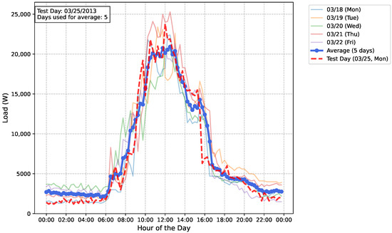
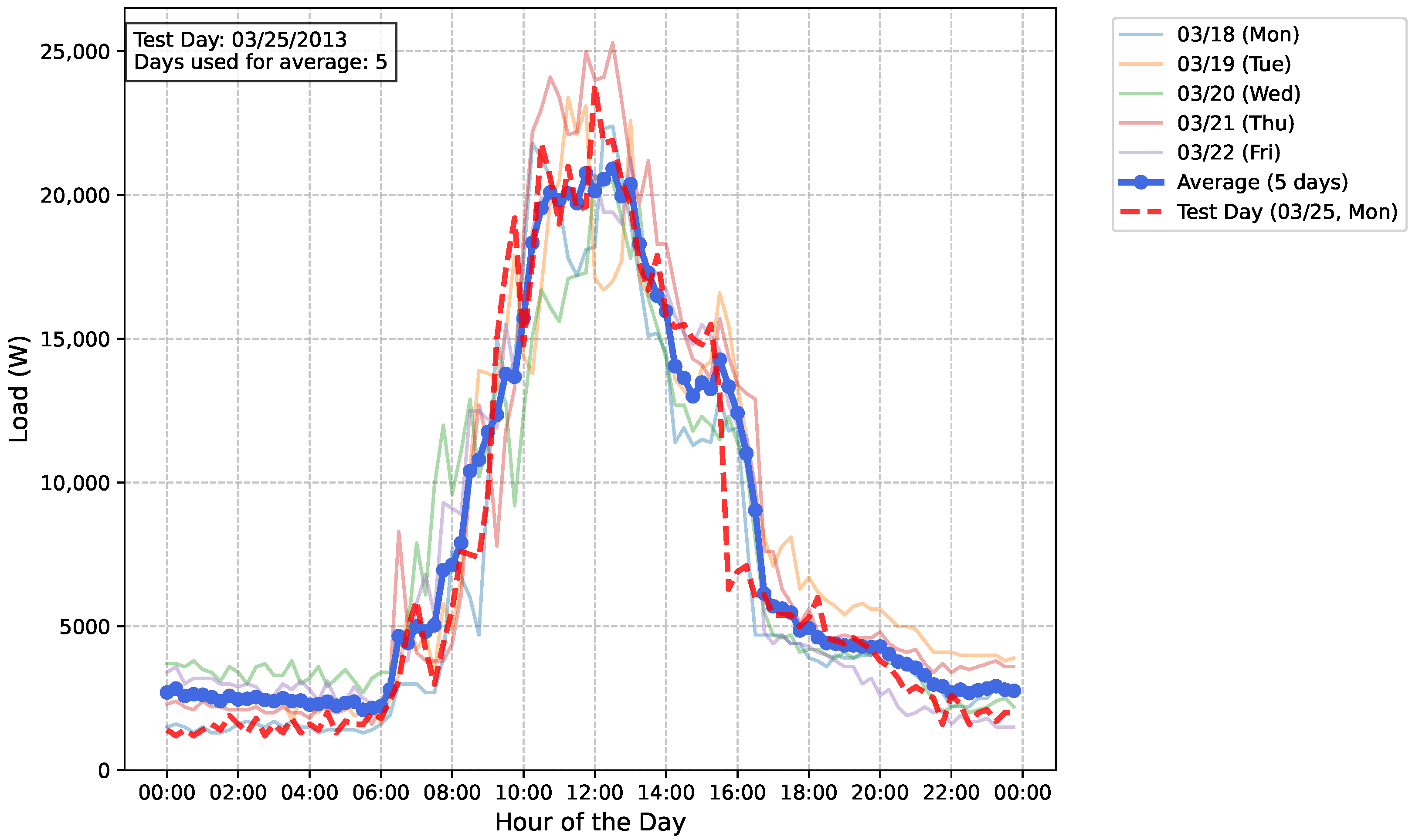
The hybrid approach uses similarity-based clustering to optimize network training. The strategy of using the average of the five preceding weekdays to identify the most similar cluster proved to be effective, as this average tends to capture the recent behavior pattern of energy consumption. This is visible in Figure 2, which compares the load curve of a test day (25 March 2013) with the load curves of the five preceding weekdays. The average curve (red dashed line) closely follows the general behavior of the test day (blue dashed line), justifying its use as a reference for clustering.

Figure 2. Load curves of previous weekdays, average and test day (25 March 2013).

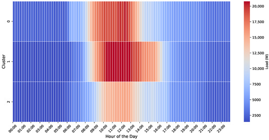
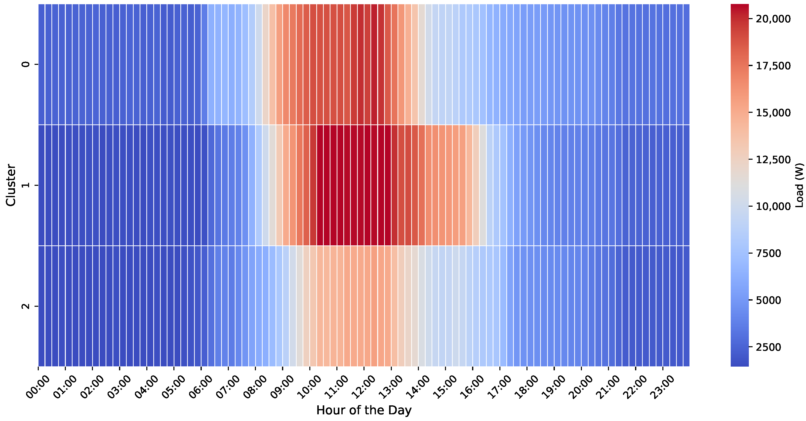
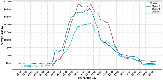
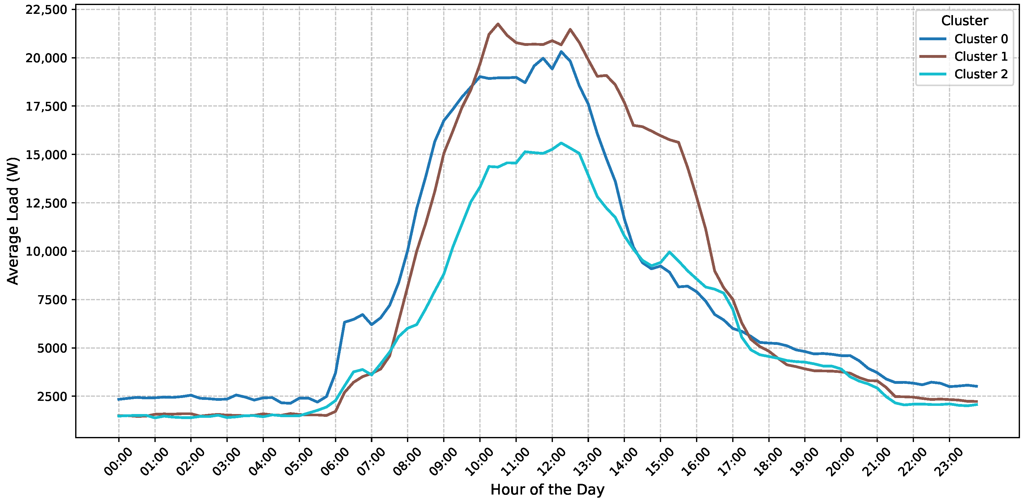
To reinforce the effectiveness of clustering, Figure 3, a heatmap, and Figure 4, a line graph, illustrate the average load profiles of the three clusters identified by the K-means algorithm for Mondays. This specific weekday was selected for detailed visualization as it typically exhibits the most pronounced consumption variability, making the clustering effect particularly evident. Cluster 1, for example, represents a significantly higher consumption pattern, with sharp peaks during business hours, especially between 9:00 a.m. and 2:00 p.m. In contrast, Cluster 2 presents a consistently lower load profile throughout the day. The clarity with which K-means separates these behaviors demonstrates that clustering organizes data so the Fuzzy ARTMAP network can learn from more homogeneous and consistent consumption profiles. The ability to identify and use these distinct patterns is a key factor in the superior performance of the hybrid model.

Figure 3. Heatmap of load behavior in clusters for Mondays.

Figure 4. Average load behavior in clusters for Mondays.

3.4. Performance Analysis and Qualitative Comparison

The following tables (Table 3 and Table 4) detail the performance metrics for a sample of days, offering a qualitative comparison between the hybrid model and the Fuzzy ARTMAP approach. We do not present detailed results for the other models (MLP and Decision Tree) here, as their performance was consistently inferior, as already demonstrated in the overall statistical analysis and in Table 1 and Table 2. This focused approach allows for a more direct and relevant validation of the contribution of clustering to the Hybrid Model.

Table 3. Forecasting results without clustering, with error metrics by date and weekday.

Weekday	Forecasted Day	MAPE (%)	RMSE (W)	MAE (W)
	04 June 2012	39.93	2948.06	2246.72
	02 July 2012	35.74	2828.97	2116.87
Monday	27 August 2012	51.25	4898.25	3362.92
	10 September 2012	24.65	2363.79	1457.81
	03 June 2013	33.82	2495.07	1728.23
	17 July 2012	28.94	3288.02	2249.38
	27 November 2012	22.04	1745.00	1378.21
Tuesday	12 March 2013	34.38	5546.29	3610.01
	14 May 2013	22.06	1574.44	1094.79
	09 July 2013	20.95	1975.82	1338.65
	23 May 2012	39.04	4617.05	3301.02
	30 May 2012	38.26	5657.40	3943.84
Wednesday	27 June 2012	49.60	3581.87	2939.55
	16 January 2013	26.70	2840.45	1917.83
	07 August 2013	21.83	2181.61	1432.81
	19 July 2012	24.84	2552.45	1681.48
	30 August 2012	30.18	4707.09	3298.65
Thursday	24 January 2013	34.26	3311.84	2461.92
	21 March 2013	26.42	3148.23	2288.22
	23 May 2013	23.48	1864.36	1145.37
	04 May 2012	31.64	4076.96	2865.26
	29 June 2012	32.49	3545.73	2770.92
Friday	27 July 2012	30.87	2828.96	2047.80
	01 February 2013	21.56	3753.42	2446.43
	01 March 2013	33.10	4872.23	3444.79

Table 4. Forecasting results using clustering, with error metrics by date and weekday.

Weekday	Test Date	MAPE (%)	RMSE (W)	MAE (W)
	04 June 2012	13.38	1224.33	819.13
	02 July 2012	14.41	2561.90	1485.13
Monday	27 August 2012	12.67	1140.37	764.38
	10 September 2012	14.99	1966.08	1201.25
	03 June 2013	20.37	2346.90	1376.15
	17 July 2012	11.81	1132.66	768.39
	27 November 2012	17.12	1775.90	1217.00
Tuesday	12 March 2013	15.94	2053.29	1228.61
	14 May 2013	16.44	1335.55	901.25
	09 July 2013	14.28	1070.11	770.94
	23 May 2012	19.98	3598.44	2153.60
	30 May 2012	14.70	2859.40	1692.77
Wednesday	27 June 2012	16.92	1972.91	1330.75
	16 January 2013	20.27	1884.29	1238.74
	07 August 2013	20.75	2213.70	1486.98
	19 July 2012	17.60	2353.28	1435.50
	30 August 2012	18.67	3145.25	1729.06
Thursday	24 January 2013	16.38	1804.37	990.95
	21 March 2013	17.01	1944.79	1241.15
	23 May 2013	15.93	1774.39	987.11
	04 May 2012	14.78	2425.45	1439.66
	29 June 2012	17.31	3117.66	1849.57
Friday	27 July 2012	14.78	1618.82	1041.61
	01 February 2013	18.86	2534.06	1575.77
	01 March 2013	20.90	2724.67	1600.83

Results Without Clustering

According to the non-clustered approach described in Section 2.5, all working days were individually forecasted using training based on random subsets of the same weekday. The results illustrate the challenges of forecasting in disaggregated environments, where the model’s performance can vary significantly across different weekdays.

The model’s performance varied significantly across the weekdays. The average MAPE values were higher on Mondays and Wednesdays, suggesting more complex consumption dynamics on those days. This behavior may be related to the resumption of activities after the weekend and the diversity of institutional routines.

Since the non-clustered approach does not perform prior similarity filtering, the presence of atypical or noisy profiles in the training set directly impacts the error metrics. This highlights the limitations of this strategy in environments with high behavioral variability. The data in Table 3 are only illustrative examples of forecasted days, as forecasting was performed for all available weekdays from Monday to Friday, as described in the methodology.

3.5. Results with Clustering

The hybrid approach optimizes the Fuzzy ARTMAP network’s training by using a preliminary clustering step. This method allows the model to learn from more homogeneous data subsets.

For each forecast, the model uses the average load curve of the five preceding weekdays to identify the most similar cluster. The Fuzzy ARTMAP network is then trained exclusively with data from that specific cluster. This process ensures that the model learns from the most relevant data, removing the test day from the training set to maintain causality.

Table 4 provides the MAPE, RMSE, and MAE values from sample test days. The data is illustrative, as the model was executed for all available weekdays to validate its robustness in disaggregated contexts.

Overall, a significant reduction in error metrics is observed compared to the non-clustered approach, especially on days with greater variability in load patterns. This result reinforces the contribution of similarity-based segmentation to model specialization and improved forecasting reliability in institutional environments with high behavioral oscillation.

3.6. General Comparison Between Approaches

This section provides a comparative analysis between forecasts performed with and without K-means clustering. We focus on the hybrid approach and the base Fuzzy ARTMAP model, as these two models consistently outperformed other methods like MLP and Decision Trees. The initial performance analysis and the Mann–Whitney U statistical test confirmed their superiority across all metrics and weekdays, justifying this focused comparison (Section 3.1 and Section 3.2).

Table 5 shows the percentage gains from applying clustering for each metric (MAPE, RMSE, and MAE). The gain was calculated based on the relative error reduction compared to the non-clustered approach, using the results from Table 3 and Table 4. The goal is to highlight the practical benefit of the segmentation strategy on forecasting effectiveness.

Table 5. Percentage gain per metric (MAPE, RMSE, and MAE) with clustering applied.

Subset	Forecasted Date	MAPE Gain (%)	RMSE Gain (%)	MAE Gain (%)
	04 June 2012	66.49	58.47	63.54
	02 July 2012	59.68	9.44	29.84
Monday	27 August 2012	75.28	76.72	77.27
	10 September 2012	39.19	16.83	17.60
	03 June 2013	39.77	5.94	20.37
	17 July 2012	59.17	65.55	65.83
	27 November 2012	22.29	−1.78	11.70
Tuesday	12 March 2013	53.65	62.98	65.97
	14 May 2013	25.48	15.17	17.68
	09 July 2013	31.84	45.83	42.40
	23 May 2012	48.83	22.07	34.74
	30 May 2012	61.56	49.47	57.09
Wednesday	27 June 2012	65.88	44.88	54.74
	16 January 2013	24.09	33.66	35.42
	07 August 2013	4.95	−1.47	−3.78
	19 July 2012	29.14	7.81	14.61
	30 August 2012	38.13	33.20	47.58
Thursday	24 January 2013	52.17	45.52	59.74
	21 March 2013	35.61	38.23	45.76
	23 May 2013	32.16	4.82	13.82
	04 May 2012	53.29	40.53	49.76
	29 June 2012	46.74	12.07	33.26
Friday	27 July 2012	52.12	42.78	49.14
	01 February 2013	12.53	32.51	35.58
	01 March 2013	36.88	44.07	53.54

Overall, applying clustering resulted in a significant reduction in error metrics, especially on dates with higher variability in load patterns. This reinforces the contribution of similarity-based segmentation to model specialization and to improving forecast reliability in dynamic institutional environments.

The strategy of dynamically identifying the most representative cluster—based on the average of the five preceding weekdays—proved effective for selecting more homogeneous subsets. This facilitated network learning with consistent patterns and mitigated the impact of outliers.

In addition to the quantitative improvement, the clustered approach also showed greater regularity, with reduced error dispersion. This stability indicates a better generalization capacity for the network, even in operational scenarios subject to unpredictable variations, such as in microgrids.

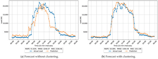
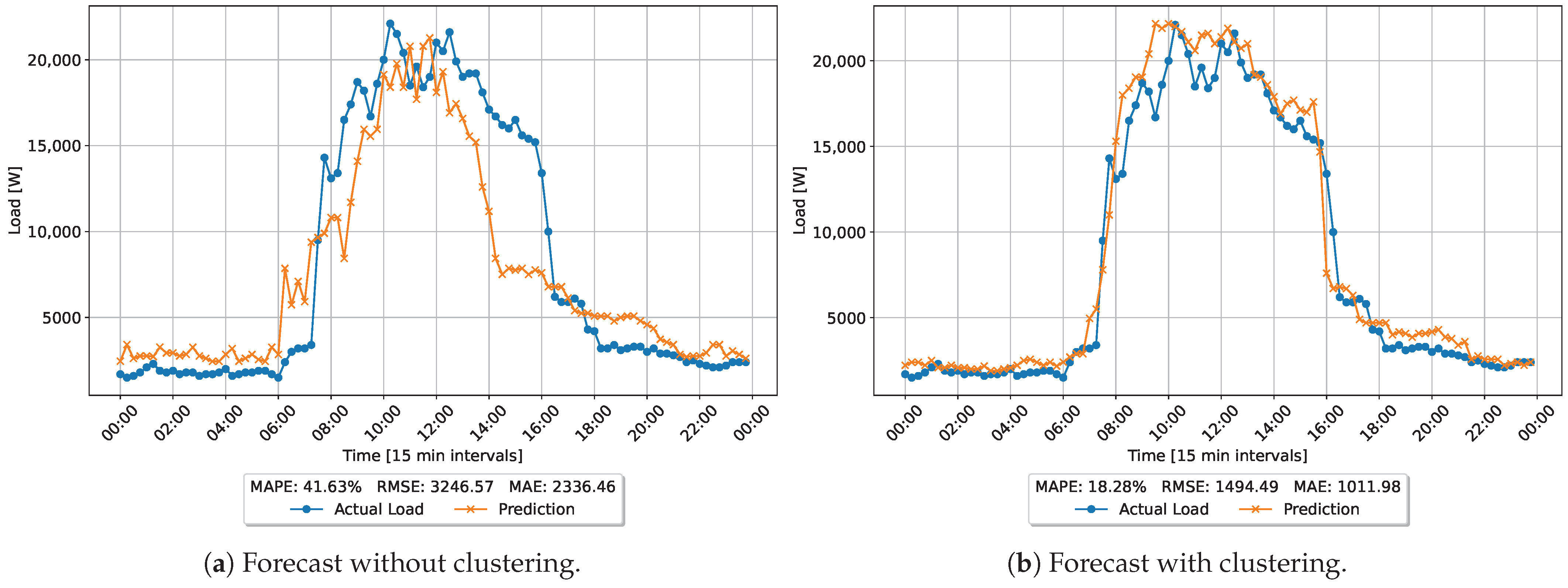
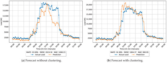
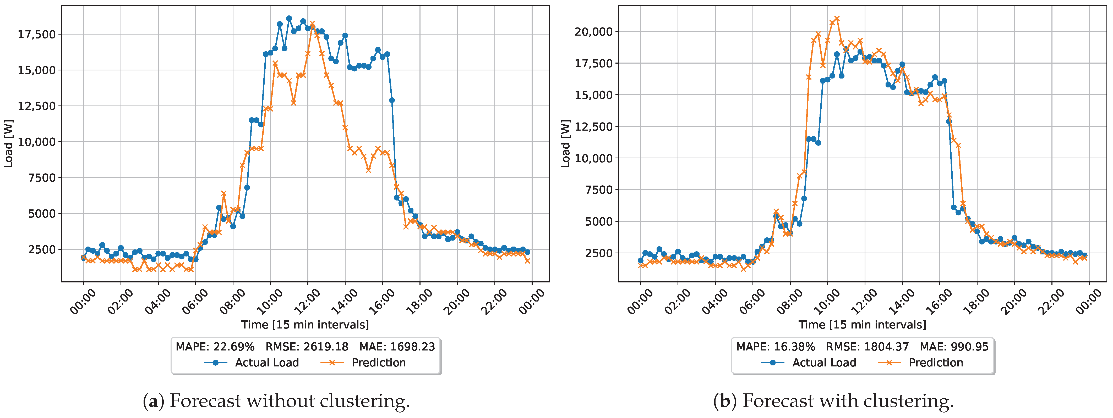
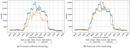
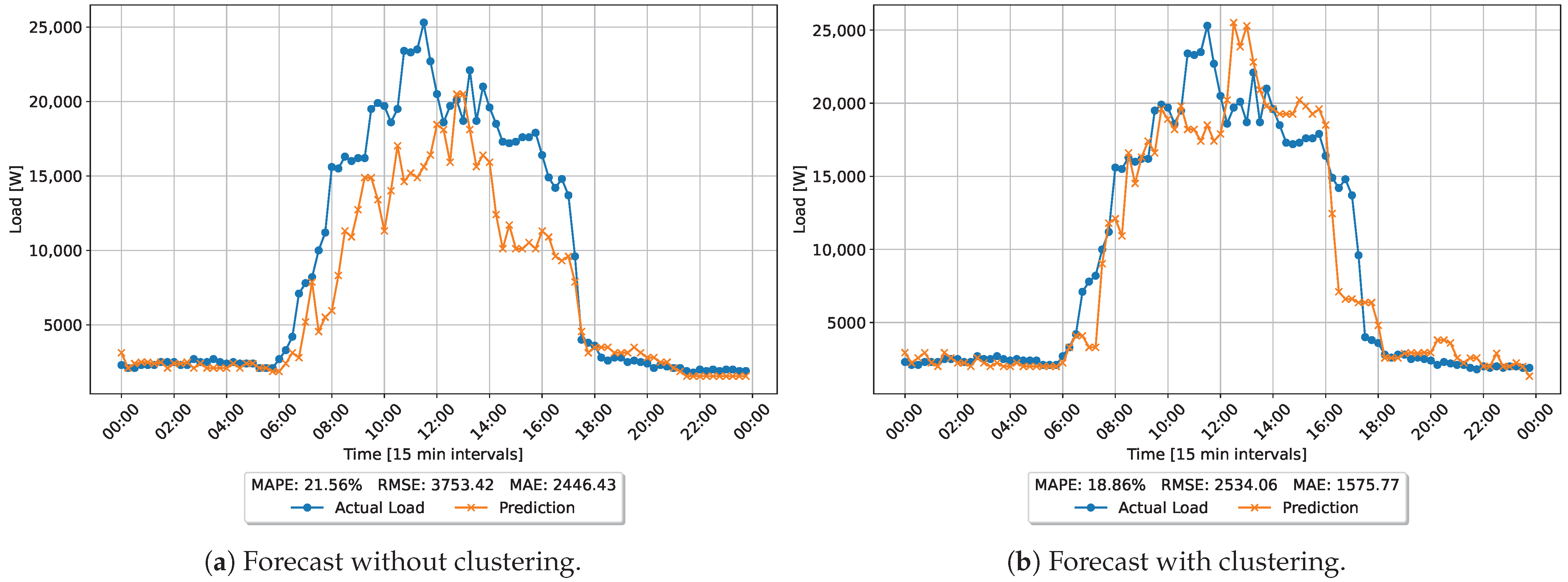
Figure 5, Figure 6 and Figure 7 visually illustrate the difference between forecasts generated by the two strategies, comparing the real profiles with the estimates obtained with and without clustering. It is clear that by grouping data by similarity, the model can reproduce the structure of the load curves more accurately.

Figure 5. Comparative analysis of load curves for 17 December 2012, Monday.

Figure 6. Comparative analysis of load curves for 24 January 2013, Thursday.

Figure 7. Comparative analysis of load curves for 1 February 2013, Friday.

This figure (Figure 5) highlights a key finding: the hybrid model’s ability to better capture the load curve’s shape explains its quantitative gains. This is particularly true for the peak load, which is a significant period for energy management.

As shown in Figure 6 and Figure 7, the hybrid model’s ability to capture load curve trends more accurately is clear across different dates. The clustered approach consistently aligns better with the actual load, showing its reliability in managing the daily variations in energy consumption.

4. Discussion

The results show that our hybrid model, which combines K-means clustering with a Fuzzy ARTMAP neural network, is an effective tool for forecasting energy consumption in environments with constantly changing patterns. Analysis across all weekdays, using multiple error metrics, reveals that the model not only surpasses the standalone Fuzzy ARTMAP network but also performs better than traditional approaches like Decision Trees and MLPs.

The model’s success lies in how clustering organizes the training process. By separating days into groups with similar consumption patterns, the Fuzzy ARTMAP network learns from a cleaner, more focused dataset. Table 1 shows this improvement through the reduction in MAPE, MAE, and RMSE values. Statistical analysis using the Mann–Whitney U test (Table 2) confirms this improvement is not coincidental. Even in the few cases where statistical significance was less pronounced, such as for the MAPE on Wednesday ($p=0.0489$), the value is still within the confidence limit, which demonstrates the model’s consistency.

A key design decision was to use the average consumption of the five previous weekdays to select the right cluster for the forecast. This method worked well because recent behavior is a great indicator of what will happen next. Figure 2 makes this clear, showing how the average curve closely approximates the actual curve of the test day. It is a simple, practical solution that allows the model to adapt to new trends without needing complex configurations.

Figure 3 and Figure 4 show why this works so well. The images reveal distinctly different consumption patterns for Mondays: some days have high, well-defined consumption peaks, while others have lower, more stable consumption. Clustering successfully separates these “types” of days, allowing the forecasting model to specialize in each one. Figure 5, Figure 6 and Figure 7 show the result of this specialization: the hybrid model’s forecasts follow the shape and peaks of the actual consumption much more faithfully than the model without clustering.

This work builds on previous research but focuses on a specific challenge: forecasting load in a real-world environment using only historical consumption data, without extra data like weather forecasts. The results show that even without this additional information, intelligently organizing the data brings great benefits. The model’s ability to handle the natural instability of this data suggests it could be useful for other forecasting problems involving complex time series, such as predicting solar power generation or demand in different types of buildings. It could even be applied to other regression tasks.

It is important to acknowledge some limitations of this study. The analysis relied solely on historical consumption, and adding information like temperature, academic calendars, or building occupancy data could make the forecasts even better. The dataset itself had flaws, such as periods of strikes and missing measurements, which, although corrected with interpolation, may have added some noise to the process. The choice of three clusters was also a practical decision to ensure that each group had enough samples for effective training; a longer data history could allow for the use of more clusters, possibly refining the forecast further. Finally, although the model was tested on all available weekdays, its performance in other locations, such as different universities or commercial buildings, still needs to be verified.

In the future, we plan to explore using smoothing techniques to filter noise from the data before applying clustering. Testing the model with external data and in other locations will be essential to confirm its practical utility in energy management. The Fuzzy ARTMAP network’s ability to learn continuously and its good tolerance for noise are features that align perfectly with this approach, allowing the model to adapt to new patterns without needing to be completely retrained.

5. Conclusions

This work proposed a hybrid model based on the integration of the Fuzzy ARTMAP neural network and K-means clustering, applied to hourly electricity load forecasting at a disaggregated level. The developed methodology stood out for its ability to dynamically identify the group most similar to the consumption profile of a given day, based on the average of the five most recent weekdays. As a result, it was possible to train the network exclusively with more homogeneous data aligned with the expected behavior, thereby improving the model’s accuracy.

It is important to highlight that the good performance obtained is not solely due to the application of clustering but also to a set of essential data preprocessing steps performed prior to modeling. These steps included the removal of load records below 5000 W, the exclusion of national and municipal holidays, the interpolation of gaps in series with missing data, and the use of cyclic encoding to represent the time variable, standardizing the curves into series with 96 daily records (15 min intervals). These actions were crucial to ensure consistency and comparability among the profiles used.

The results showed significant improvements across the MAPE, RMSE, and MAE metrics, outperforming not only the non-clustered approach but also other established models like MLP and Decision Trees. The statistical significance of these improvements was confirmed by the Mann–Whitney U test, validating the superiority of the hybrid architecture. Furthermore, the model exhibited robustness in the face of behavioral fluctuations typical of institutional microgrids, even when operating without external variables such as temperature or occupancy. The adopted structure proved promising for real environments with incomplete or difficult-to-standardize data, contributing methodologically to the literature in the field.

However, the study presented significant limitations. The available dataset contained only load and timestamp (date and time) information, without additional explanatory variables. The analyzed period coincided with moments of academic instability (such as strikes), which affected consumption patterns, making each day potentially atypical even within the same weekday subset. The dataset also presented failures and missing data, requiring interpolation techniques for gap filling. Moreover, the intrinsic challenge of working with disaggregated loads, characterized by high noise and irregular behavior, imposes additional barriers to modeling. Nevertheless, the MAPE values observed are considered satisfactory given the complexity of the scenario.

For future developments, it is suggested to integrate smoothing techniques into the preprocessing pipeline, with the goal of reducing high-frequency noise and improving signal continuity. Additionally, applying the model to different institutional environments and with varying levels of aggregation may help assess its generalization capacity and expand its practical applicability.

References

- Heghedus, C.; Chakravorty, A.; Rong, C. Energy Load Forecasting Using Deep Learning. In Proceedings of the 2018 IEEE International Conference on Energy Internet (ICEI), Beijing, China, 21–25 May 2018; pp. 146–151. [Google Scholar] [CrossRef] [Scilit]
- Ghelardoni, L.; Ghio, A.; Anguita, D. Energy Load Forecasting Using Empirical Mode Decomposition and Support Vector Regression. IEEE Trans. Smart Grid 2013, 4, 549–556. [Google Scholar] [CrossRef] [Scilit]
- Saber, A.Y.; Alam, A.K.M.R. Short term load forecasting using multiple linear regression for big data. In Proceedings of the 2017 IEEE Symposium Series on Computational Intelligence (SSCI), Honolulu, HI, USA, 27 November–1 December 2017; pp. 1–6. [Google Scholar] [CrossRef] [Scilit]
- Hernández, L.; Baladrón, C.; Aguiar, J.M.; Carro, B.; Sánchez-Esguevillas, A.; Lloret, J. Artificial neural networks for short-term load forecasting in microgrids environment. Energy 2014, 75, 252–264. [Google Scholar] [CrossRef] [Scilit]
- Panapakidis, I.P.; Dagoumas, A.S. Day-ahead electricity price forecasting via the application of artificial neural network based models. Appl. Energy 2016, 172, 132–151. [Google Scholar] [CrossRef] [Scilit]
- Kouzelis, K.; Bak-Jensen, B.; Mahat, P.; Pillai, J.R. A simplified short term load forecasting method based on sequential patterns. In Proceedings of the IEEE PES Innovative Smart Grid Technologies Conference Europe, Istanbul, Turkey, 12–15 October 2014; pp. 1–5. [Google Scholar] [CrossRef] [Scilit]
- Mori, H.; Yuihara, A. Deterministic annealing clustering for ANN-based short-term load forecasting. IEEE Trans. Power Syst. 2001, 16, 545–551. [Google Scholar] [CrossRef] [Scilit]
- Cecati, C.; Kolbusz, J.; Różycki, P.; Siano, P.; Wilamowski, B.M. A Novel RBF Training Algorithm for Short-Term Electric Load Forecasting and Comparative Studies. IEEE Trans. Ind. Electron. 2015, 62, 6519–6529. [Google Scholar] [CrossRef] [Scilit]
- Müller, M.R.; Gaio, G.; Carreno, E.M.; Lotufo, A.D.P.; Teixeira, L.A. Electrical load forecasting in disaggregated levels using Fuzzy ARTMAP artificial neural network and noise removal by singular spectrum analysis. SN Appl. Sci. 2020, 2, 1218. [Google Scholar] [CrossRef] [Scilit]
- Grossberg, S. A path toward explainable AI and autonomous adaptive intelligence: Deep learning, adaptive resonance, and models of perception, emotion, and action. Front Neurorobot 2020, 14, 36. [Google Scholar] [CrossRef] [Scilit] [PubMed]
- Carpenter, G.; Grossberg, S.; Markuzon, N.; Reynolds, J.; Rosen, D. Fuzzy ARTMAP: A neural network architecture for incremental supervised learning of analog multidimensional maps. IEEE Trans. Neural Netw. 1992, 3, 698–713. [Google Scholar] [CrossRef] [Scilit] [PubMed]
- Carpenter, G.; Grossberg, S. A self-organizing neural network for supervised learning, recognition, and prediction. IEEE Commun. Mag. 1992, 30, 38–49. [Google Scholar] [CrossRef] [Scilit]
- Bergstra, J.; Bengio, Y. Random Search for Hyper-Parameter Optimization. J. Mach. Learn. Res. 2012, 13, 281–305. [Google Scholar]
- Hyndman, R.J.; Koehler, A.B. Another look at measures of forecast accuracy. Int. J. Forecast. 2006, 22, 679–688. [Google Scholar] [CrossRef] [Scilit]
- Pedregosa, F.; Varoquaux, G.; Gramfort, A.; Michel, V.; Thirion, B.; Grisel, O.; Blondel, M.; Prettenhofer, P.; Weiss, R.; Dubourg, V.; et al. Scikit-learn: Machine Learning in Python. J. Mach. Learn. Res. 2011, 12, 2825–2830. [Google Scholar]
Disclaimer/Publisher’s Note: The statements, opinions and data contained in all publications are solely those of the individual author(s) and contributor(s) and not of MDPI and/or the editor(s). MDPI and/or the editor(s) disclaim responsibility for any injury to people or property resulting from any ideas, methods, instructions or products referred to in the content. |
© 2026 by the authors. Licensee MDPI, Basel, Switzerland. This article is an open access article distributed under the terms and conditions of the Creative Commons Attribution (CC BY) license.