


Abstract
With the increasing occurrence of extreme high-temperature weather events, the traditional bundled operation of wind power (WP), photovoltaic power (PV), and pumped storage hydropower (PSH) is facing dual challenges, namely intensified renewable energy fluctuations and insufficient flexible regulation capability of PSH. Therefore, this paper proposes an optimal scheduling strategy for bundled operation based on capacity interval matching of PSH with WP and PV under extreme high-temperature weather. First, typical scenarios are generated based on a Time-series Generative Adversarial Network (TimeGAN), and an interval matching transaction model is established based on the forecast intervals of WP and PV capacity and the corrected intervals of PSH capacity. Second, considering PSH as an independent market entity, a bi-level optimization model is constructed, in which the upper-level objective is to maximize the revenue of PSH, while the lower-level objective is to minimize the total cost of the joint clearing of the energy and ancillary service markets. Finally, simulation case studies verify that under extreme high-temperature weather, the proposed optimal scheduling method increases the bundled operation capacity by 17.9% and improves the revenue of PSH in the reserve ancillary service market by 14.8%, thereby effectively enhancing the economic performance of PSH while ensuring the safe and stable operation of the system.
1. Introduction
In recent years, with the increasing occurrence of extreme high-temperature events caused by global climate warming, tremendous challenges have been posed to new power systems with a large share of renewable energy such as WP and PV. Meanwhile, the continuous development of green and sustainable energy technologies has further highlighted the importance of improving energy utilization efficiency and promoting environmentally friendly energy applications [1]. Extreme high-temperature weather is characterized by a wide impact range and long duration. As a flexible regulating power source with high technological maturity and good economic performance, PSH can mitigate the fluctuations of WP and PV, reduce the penalty costs caused by renewable energy forecasting errors, and provide reserve capacity for the reserve ancillary service market under extreme high-temperature weather [2,3]. Therefore, it is of great significance to explore the bundled operation of PSH with WP and PV under extreme high-temperature weather so as to mitigate renewable energy fluctuations and improve the operational safety and stability of new power systems.
At present, extensive research has been conducted by scholars at home and abroad on the bundled operation of WP, PV, and PSH. The bundled operation of PSH with renewable energy can improve renewable energy consumption and reduce the output fluctuations of renewable energy. Ref. [4] established a multi-objective optimization model for a bundled operation system of PSH, WP, and PV and verified that PSH can mitigate the output fluctuations of WP and PV while improving system economy and renewable energy integration. Ref. [5] addressed the optimal scheduling problem of a bundled operation system comprising WP, PV, and PSH by constructing a mixed-integer programming model considering imbalance penalties, thereby maximizing the total revenue of the joint system. Ref. [6] proposed a numerical model for a hybrid system incorporating the stochastic fluctuations of WP and the dynamic regulation of PSH and verified that the bundled operation of PSH and WP can improve the consumption rate of WP. Ref. [7] introduced a voltage source converter-based multi-terminal DC transmission system into a complementary generation system of PSH, WP, and PV, thereby promoting the role of PSH in smoothing the output fluctuations of WP and PV and reducing system revenue losses. Ref. [8] proposed an optimal scheduling model for the joint operation of WP and a PSH station considering WP forecasting errors and hydraulic constraints, which significantly mitigated WP fluctuations and improved system revenue. However, the above studies only considered capacity bundling of PSH with WP and PV in a passive dispatch mode and paid relatively little attention to the revenue analysis of PSH stations as participants in joint operation, which to some extent hinders the further development of bundled operation systems of WP, PV, and PSH. Ref. [9] constructed a bundled revenue allocation model for WP and PSH based on the Shapley value method and improved economic benefits by considering the contribution of PSH to WP consumption. Ref. [10] established an optimization model based on Nash bargaining theory for the joint participation of a wind–solar–hydro–storage complementary system in the energy and frequency regulation markets, and the case study showed that joint operation can effectively improve the revenues of all participants and the renewable energy consumption rate. Ref. [11] proposed an operating strategy for a PV–hydropower–PSH joint system participating in the electricity market, adopted scenario-based stochastic optimization to handle uncertainty, and introduced conditional value at risk to measure risk, thereby improving the operating revenues of PSH and other participants. Ref. [12] treated the bundled operation system of WP and PSH as an integrated energy aggregator participating in the electricity market and constructed an IGDT-DRO joint optimization model considering multiple uncertainties, which significantly improved the revenue of PSH. Temperature is an important factor affecting the operating state of large hydraulic structures [13]. Extreme high-temperature weather can affect the operating conditions of PSH reservoirs and, in turn, influence the operation of PSH units. Although these studies considered the role of bundled operation between PSH and renewable energy in enhancing the revenue of PSH, they did not consider the impacts of extreme high-temperature weather on the participation of PSH in bundled operation and on its revenue. The traditional bundled operation system of PSH with WP and PV cannot fully reflect the value of PSH in bundled operation under extreme high-temperature weather, thereby weakening the willingness of PSH to participate in bundled operation with WP and PV.
PSH can not only obtain revenue through bundled operation with renewable energy but also participate in electricity market clearing as a market entity [14]. At present, PSH is still mostly compensated through electricity quantities participating in the electricity market to obtain the energy price, while the capacity part is compensated according to the approved capacity tariff. However, with the development and maturation of the electricity market, the capacity tariff will be gradually weakened and eventually abolished, and it has become an inevitable trend for PSH to participate in electricity market transactions as an independent market entity [15]. Ref. [16], focusing on the revenue issue of PSH stations in the context of electricity market reform, established a phased full-life-cycle evaluation model, which facilitates the smooth transition of PSH toward becoming an independent market entity. Ref. [17], based on the bidding strategy problem of PSH participating in the energy market, constructed a stochastic optimization model with downside-risk constraints to ensure the stability of PSH revenue. Ref. [18], under the premise that PSH does not submit quantity or price bids, directly determined the optimal charging and discharging decisions according to the current state of charge and forecasted electricity prices, thereby maximizing station operating revenue and improving operational efficiency. Ref. [19] constructed a clearing model for PSH participating in the energy market to analyze the influence of different bidding strategies on its revenue, and the case study showed that the participation of PSH in the energy market can increase its revenue and reduce system costs. The above studies mainly focus on PSH participating only in transactions in the energy market. As a flexible regulating resource with fast response capability and large-scale energy storage characteristics, the value of PSH lies not only in peak-valley arbitrage in the energy market but also in providing ancillary services such as frequency regulation, reserve, and ramping for the power system [20]. Ref. [21] established a bi-level capacity allocation model for PSH participating in multiple markets. Through joint optimization of the energy and ancillary service markets, the revenue of PSH was significantly improved compared with that under the two-part tariff. Ref. [22] constructed a day-ahead scheduling optimization model for PSH participating in the joint clearing of the energy market and reserve ancillary service market based on neural-network constraints, achieving revenue maximization in the joint clearing process. Ref. [23] incorporated PSH into the security-constrained unit commitment framework and jointly cleared it with conventional units in the energy and ancillary service markets to satisfy both system load and reserve requirements. Most of the above studies are based on a mode in which PSH participates in the joint clearing of the energy market and the ancillary service market. Under extreme high-temperature weather, the system demand for reserve capacity rises significantly, whereas the fixed compensation price of PSH lacks flexibility, making it difficult to effectively incentivize PSH to increase its reserve capacity bids.
In summary, existing studies still show insufficient research on PSH operation under extreme high-temperature weather, bundled trading mechanisms, and the bidding strategy of PSH in the reserve ancillary service market. Therefore, this paper systematically carries out the following research: (1) reservoir storage variation, water level variation, hydraulic head loss, and the reduction in available unit capacity caused by evaporation are incorporated into the PSH modeling process, and the corrected available capacity is further used to adjust the declarable capacity interval of PSH when participating in bundled operation with WP and PV; (2) a capacity interval matching mechanism is proposed, under which PSH, WP, and PV participate in bundled operation through quantity-price bidding under extreme high-temperature weather, thereby enhancing the willingness of PSH to participate in bundled operation; and (3) a reserve bidding strategy for PSH considering the value of lost load is constructed to fully reflect its reserve value under extreme high-temperature conditions and further improve the total revenue of PSH.
2. Capacity Interval Matching for the Bundled Operation of PSH with WP and PV Under Extreme High-Temperature Scenarios
2.1. Framework for Bundled Operation of PSH with WP and PV Under Extreme High-Temperature Weather
Under extreme high-temperature weather, PSH participates in the bundled operation with WP and PV while simultaneously engaging in power market clearing. Extreme high-temperature weather refers to conditions in which the daily maximum temperature exceeds 35 °C for three consecutive days or longer [24], and the basic operating framework is shown in Figure 1. PSH, WP, and PV conduct day-ahead trading of bundled capacity through a capacity trading platform, with a scheduling horizon of 24 h and a time resolution of 1 h.
Figure 1.
Framework diagram of the bundled operation system of PSH with WP and PV.
Extreme high-temperature weather increases the output variability of WP and PV, thereby requiring a higher capacity level to be bundled with PSH. In the day-ahead scheduling stage, the participants in the bundled operation of PSH with WP and PV submit their bidding information, including capacity quantities and price information for both buying and selling, to the capacity trading platform. The bundled capacity transaction is then completed on the platform through a capacity interval matching method, thereby forming the day-ahead schedule for the bundled operation of PSH with WP and PV. Meanwhile, extreme high-temperature weather may lead to surging electricity demand and increased reserve requirements on the load side. As a participant in the power market, PSH takes part in the joint clearing of the energy market and the reserve ancillary service market through quantity-price bidding, thereby mitigating the impacts of extreme weather on power system operation.
2.2. Typical WP–PV–Load Scenarios Under Extreme High-Temperature Weather Based on Meteorological Factor Coupling
2.2.1. TimeGAN Model
Under extreme high-temperature weather, it is crucial to jointly model the multi-source time-series data composed of WP output, PV output, load, and related meteorological factors. These data generally exhibit characteristics such as inter-variable coupling relationships, strong nonlinearity, and complex temporal dependencies. Therefore, the generated samples are required to remain consistent with the original data in terms of both statistical distributions and dynamic temporal characteristics. Generative Adversarial Networks (GANs) are capable of generating samples with fine details and high resolution. A GAN consists of a generator and a discriminator and generates samples that approximate the original data through adversarial learning between the two components. However, when generating time-series data, traditional GANs often have difficulty in effectively modeling the short-term and long-term dependencies in the data and cannot accurately fit the conditional probability distribution of the original data, resulting in generated sequences that lack realism and consistency.
TimeGAN is a GAN-based model for time-series generation proposed by [25]. Built upon the conventional GAN framework, this model introduces a self-supervised mechanism and a feature-matching strategy. It is capable not only of generating high-quality synthetic time-series data but also of preserving the temporal dependency characteristics of the original data in the generated sequences [26]. The TimeGAN model consists of four core network components, namely, an embedding network, a discriminator network, a generator network, and a recovery network. Among them, the generator network and the discriminator network constitute the adversarial learning component of TimeGAN, while the embedding network and the recovery network form the autoencoding component of the model, enabling a reversible mapping between features and the latent space. The overall architecture of the TimeGAN model is shown in Figure 2.
Figure 2.
Architecture of the TimeGAN model.
TimeGAN first employs the embedding network to map the original time series into the latent space, so as to capture their temporal dependency features. It then generates new sequences in the latent space and reconstructs them back to the original space through the recovery network. Finally, by integrating a supervised learning mechanism with adversarial training, TimeGAN ensures that the generated samples are highly consistent with the real data in terms of both data distribution and dynamic temporal structure. Its core procedure includes the following steps:
(1) Embedding and generation module: Let the input time series of the original data be , , where denotes the observed value of variable at time . TimeGAN maps the original sequence into a latent vector sequence , through the embedding network, which can be expressed as follows:
where denotes the parameters of the embedding network.
After the embedding network completes feature extraction from the real data, TimeGAN enters the generation stage, in which the generator outputs a generated latent sequence with the same dimensionality as the real embedded sequence:
where denotes the latent vector representation generated at time , and denotes the parameters of the generator.
After the generation process is completed, the recovery network further decodes the latent-space sequence output by the generator and maps it back to the original feature space through a nonlinear transformation, thereby generating a synthetic original feature sequence:
where denotes the latent vector representation generated at time , and denotes the parameters of the recovery network.
(2) Supervised mechanism design: The supervisor module is used to model the temporal dependencies in the latent space. In the initial stage, the real latent vectors are taken as the training targets, and the latent state at the current time step is used as the input to predict the latent state at the next time step:
where denotes the latent vector representation at time , and denotes the parameters of the supervisor.
(3) Loss function construction: In the first step, the self-supervised loss is used to train the supervisor. By minimizing the mean squared error between the real latent states and the predicted latent states, the model is encouraged to learn the stepwise dynamic relationships of the data in the latent space, thereby effectively capturing the temporal dependency structure. In the second step, the reconstruction loss is used to train the embedding network and the recovery network. By measuring the reconstruction error between the original input and the decoded output, it ensures that the latent space preserves the key information of the original data. In the third step, the discriminator loss maximizes the discriminator’s ability to distinguish between real latent states and generated latent states, while the generator loss minimizes the discriminator’s classification accuracy. Together, these two losses constitute the adversarial loss. Finally, TimeGAN forms a joint loss function as the overall optimization objective by taking a weighted sum of the self-supervised loss, reconstruction loss, and generator loss. The corresponding function expressions are given as follows:
where denotes the self-supervised loss function; denotes the real latent vector representation at time ; denotes the reconstruction loss; denotes the original input sequence at time ; denotes the adversarial loss function of the discriminator; denotes the adversarial loss function of the generator; denotes the distribution of real latent variables; denotes the distribution of generated latent variables; denotes the joint loss function; and , , and denote the weighting parameters of the self-supervised loss, reconstruction loss, and generator loss, respectively.
The TimeGAN model is a deep learning model. In this study, it is constructed using a Gated Recurrent Unit (GRU) recurrent neural network. The training process of TimeGAN is divided into two stages:
Stage 1: Joint training of the embedding network and recovery network.
Objective: To enable the embedding network and the recovery network to accurately accomplish the mapping and reconstruction from the original time series of temperature, wind speed, solar irradiance, and load to the latent space and then from the latent space back to the original feature space. This ensures that the latent representations have good structure-preserving capability and provides a reliable low-dimensional feature basis for subsequent generation tasks.
Step 1: Input the original time-series data of temperature, wind speed, solar irradiance, and load into the embedding network to obtain the corresponding latent vector representations in the latent space;
Step 2: Feed the latent vectors in the latent space into the recovery network to reconstruct the original data of temperature, wind speed, solar irradiance, and load, obtain the reconstructed sequence, and calculate the reconstruction loss;
Step 3: Take the next-time-step state of the real latent vectors as the supervised target, constrain the output of the supervisor, and calculate the self-supervised loss so as to enhance the model’s ability to learn temporal dependencies;
Step 4: Update the parameters of the embedding network, recovery network, and supervisor according to the combined results of the reconstruction loss and the self-supervised loss;
Step 5: Repeat the above process until the model reaches the preset number of training epochs for the current stage or the loss function converges.
Stage 2: Adversarial training of the generator, supervisor, and discriminator.
Objective: To enable the generator to produce latent features that are consistent with the distribution of real data while also exhibiting reasonable temporal evolution patterns. The discriminator is used to distinguish real samples of temperature, wind speed, solar irradiance, and load from the generated samples of temperature, wind speed, solar irradiance, and load, thereby driving the generator to continuously improve its generation capability.
Step 1: Sample from the random noise distribution and feed the samples into the generator to obtain the generated latent vector sequence in the latent space;
Step 2: Input the generated latent vectors into the supervisor to constrain their temporal evolution, so that the generated sequences of temperature, wind speed, solar irradiance, and load maintain reasonable dynamic continuity between adjacent time steps;
Step 3: Feed the real latent vector sequence and the generated latent vector sequence into the discriminator, respectively, obtain the corresponding discrimination results, and calculate the adversarial loss;
Step 4: Further input the generated latent vectors into the recovery network to obtain the generated original feature sequence;
Step 5: Construct a joint loss function by combining the self-supervised loss, reconstruction loss, and adversarial loss and alternately update the parameters of the generator, supervisor, discriminator, and recovery network;
Step 6: Repeat the above training process until the model reaches the preset number of training iterations and converges.
Training ends.
2.2.2. Joint WP–PV–Load Scenario Generation Under Extreme High-Temperature Weather Based on Coupled Meteorological Factors
A clustering algorithm is employed to classify extreme high-temperature weather according to temperature. A robust weighted K-means algorithm is employed to cluster extreme high-temperature samples characterized by temperature, where each sample is represented by its temperature feature [27]. The objective is to increase the similarity of temperature samples within the same cluster while enlarging the differences among different clusters, thereby identifying the potential intensity differences among extreme high-temperature samples. The Davies–Bouldin Index (DBI) is employed to quantitatively analyze the number of clusters in the robust weighted K-means algorithm. DBI evaluates clustering quality by calculating the ratio of intra-cluster dispersion to inter-cluster separation. A smaller DBI value indicates better clustering performance, namely, higher compactness of samples within each cluster and clearer separation between different clusters. The definition of DBI includes the following:
(1) Intra-cluster dispersion.
denotes the arithmetic mean of the distances between all sample points in the -th cluster and its centroid. A smaller value of indicates better clustering performance, meaning that the elements within the cluster are more compact. The calculation formula of is as follows:
where denotes the -th cluster; denotes the centroid of ; and denotes the distance between data point and . When , the Euclidean distance is adopted.
(2) Inter-cluster separation.
denotes the Euclidean distance between the centroid of the -th cluster and that of the -th cluster. A smaller value of indicates better clustering performance, while a larger value of represents a higher degree of separation between clusters. The calculation formula of is as follows:
(3) Cluster similarity.
measures the degree of similarity between clusters. A smaller value of indicates better clustering performance. The calculation formula of is as follows:
(4) Maximum cluster similarity.
For each cluster , the cluster with the largest is identified and denoted as follows:
(5) DBI.
DBI is defined as the arithmetic mean of the maximum similarities of all clusters. A smaller DBI value indicates better clustering performance, meaning that the data points within each cluster are more compact and the separation between clusters is higher. The calculation formula of DBI is as follows:
During the clustering analysis process, clustering is performed repeatedly under different values of , and the DBI metric corresponding to each is evaluated. The value of corresponding to the minimum DBI is ultimately selected as the optimal number of clusters.
The main procedure of the robust weighted K-means algorithm includes cluster center initialization, calculation of weights according to the distances between samples and the cluster centers or the reference median, sample assignment under the effect of the weights, updating of cluster centers, and finally determination of whether the iteration should terminate based on the convergence condition. The specific procedure is shown in Figure 3.
Figure 3.
Flowchart of the robust weighted K-means clustering algorithm.
Based on the historical data from a region in Sichuan Province, this paper determines the optimal value of using the DBI metric, and the corresponding DBI results are shown in Figure 4.
Figure 4.
DBI selection for the temperature factor.
As can be seen from Figure 4, the DBI curve of temperature reaches its minimum at ; therefore, the optimal value of is selected as 2. Furthermore, clustering is performed with , and a statistical analysis of the clustering results shows that one category of samples exhibits generally higher temperatures, while the other category exhibits relatively lower temperatures, with the boundary located close to 38 °C. On this basis, this paper defines extreme high-temperature weather with a maximum temperature above 38 °C as the High-Temperature A scenario and that with a maximum temperature of 38 °C or below as the High-Temperature B scenario.
A joint scenario generation model for temperature, wind speed, solar irradiance, and load is constructed using the TimeGAN model. After generating multi-source meteorological data that conform to real temporal characteristics, the generated meteorological data are further converted into WP and PV output data, thereby constructing meteorologically coupled joint WP–PV–load scenarios under different types of extreme high-temperature weather. The specific procedure is shown in Figure 5.
Figure 5.
Flowchart of meteorologically coupled WP–PV joint output scenarios.
Ref. [28] adopted the WT and PV output conversion models. WP output is strongly correlated with wind speed, and the WP output model can be expressed in terms of its relationship with wind speed as follows:
The output power of PV generation is mainly determined by the surface temperature of the PV modules and the solar irradiance. Within the rated power range, the expression for PV output is given as follows:
2.2.3. PSH Evaporation Model and Bundled Operation Capacity Intervals Based on Similar Days Identified by DTW
The DTW algorithm is a method for measuring the similarity between two time series [29]. Given two time series and , a distance matrix is constructed, where denotes the Euclidean distance between and . The objective of DTW is to find an optimal warping path such that the cumulative distance from point to point is minimized, where denotes the number of point pairs in path . The warping path is required to satisfy three constraints: (1) boundary condition: and ; (2) continuity: if , then the next path point must satisfy and ; and (3) monotonicity: if , then the next path point must satisfy and . The DTW distance is given as follows:
where denotes the -th path element of path .
Combined with the Penman formula model in Ref. [30], after obtaining the relevant meteorological data of similar days based on the DTW algorithm, the evaporation of both the upper and lower reservoirs of PSH is calculated using the Penman formula. This method can comprehensively reflect the combined effects of meteorological conditions and aerodynamic processes on evaporation. The specific expression is as follows:
where denotes the wind speed function of PSH unit during period ; denotes the saturated vapor pressure of PSH unit during period ; denotes the actual vapor pressure of PSH unit during period ; and denotes the reservoir heat storage variation of PSH unit during period .
As air moves from land to the water surface, the evaporation effect is weakened due to the increase in humidity, and the wind speed function is therefore formulated as follows:
where denotes the characteristic length of the reservoir, and denotes the wind speed of PSH unit during period .
The storage capacities of the upper and lower reservoirs are affected by water evaporation, and the variation in the reservoir storage capacity of PSH within each period is expressed as follows:
where and denote the storage capacities of the upper and lower reservoirs of PSH unit during period , respectively; and denote the storage capacities of the upper and lower reservoirs of PSH unit during period , respectively; and denote the water volumes for pumping and power generation of PSH unit during period , respectively; and denote the evaporation rates of the upper and lower reservoirs of PSH unit during period , respectively; and and denote the surface areas of the upper and lower reservoirs of PSH unit during period , respectively.
By referring to the water level–storage capacity relationship curves of the upper and lower reservoirs, the water levels during period can be obtained. Accordingly, the variation in the hydraulic head considering the effect of evaporation on reservoir storage capacity can be further determined, which can be expressed as follows:
where denotes the hydraulic head variation of PSH unit during period ; and denote the water levels of the upper and lower reservoirs of PSH unit during period without considering the effect of evaporation, respectively; and and denote the water levels of the upper and lower reservoirs of PSH unit during period when the effect of evaporation is taken into account, respectively.
According to the hydraulic head variation, the reduced capacity of PSH during period can be obtained as follows:
To avoid a mismatch between the cleared quantity of PSH in the power market and its actual available capacity under extreme high-temperature weather, which may be caused by variations in hydraulic head and reservoir operating constraints, the capacity reduction of PSH due to high temperature is accounted for through the capacity interval matching transaction of PSH with WP and PV. Specifically, the actual declared upper bound of the PSH capacity interval is determined by subtracting the reduced PSH capacity from the originally scheduled upper bound of the declared capacity interval. Accordingly, the actual declared capacity interval can be expressed as follows:
where denotes the capacity interval of PSH for bundled operation with WP and PV during period ; and denote the upper and lower bounds of the declared capacity interval of PSH for bundled operation with WP and PV power during period , respectively; and and denote the upper and lower bounds of the originally planned declared capacity interval of PSH for bundled operation with WP and PV power during period , respectively.
The novelty of this part lies in integrating the effect of evaporation-induced reservoir storage change, water-level variation, hydraulic-head loss, and actual capacity reduction into a unified modeling chain and further transmitting this capacity reduction to the correction of the declared bundled-operation capacity interval of PSH.
2.2.4. Bundled Operation Capacity Interval Matching Considering WP and PV Uncertainty Under Extreme High-Temperature Weather
By constructing meteorologically coupled joint typical wind–solar–load scenarios under extreme high-temperature weather, a typical day is selected for the day-ahead scheduling of wind–solar and PSH bundled operation. However, under extreme high-temperature weather, random disturbances are relatively pronounced. Meanwhile, excessively high temperatures may reduce the operating efficiency of WP and PV units, causing the actual WP and PV output to deviate further from the forecasted wind–solar output, thereby making it difficult to fully characterize the uncertainty of WP and PV output under extreme high-temperature weather. Therefore, this section adopts an interval forecasting method. According to the quantile results of PV and WP at different confidence levels and , the output intervals of PV and WP are respectively expressed as follows:
where and denote the output intervals of PV unit and WP unit , respectively; and denote the baseline values of PV unit and WP unit , respectively; and denote the quantile results of probabilistic forecasting at quantile levels and , respectively; and and denote the quantile results of probabilistic forecasting at quantile levels and , respectively.
During the day-ahead scheduling stage for the joint operation of WP, PV, and PSH, the upper and lower quantile bounds of the forecast intervals for WP and PV output are obtained for PV and WP, respectively, according to the quantile results at different confidence levels and . These intervals are then taken as the upper and lower bounds of the capacity intervals that PV and WP require for bundled operation with PSH, so that the bundled operation capacity can cover the fluctuations caused by WP and PV output uncertainty under the preset confidence levels.
Under the traditional bundled operation mode of PSH with WP and PV in extreme high-temperature weather, PSH is unable to reserve sufficient capacity for bundled operation with WP and PV due to factors such as reduced hydraulic head, reservoir operating constraints, prolonged continuous operation, and the volatility and uncertainty of WP and PV output. Meanwhile, because extreme high-temperature weather leads to higher electricity prices, PSH may become less willing to participate in bundled operation with WP and PV in pursuit of greater profits, thereby reducing the capacity allocated to bundled operation. If only the traditional bundled operation mode of PSH with WP and PV is adopted, it is difficult to fully reflect the system regulation costs and flexibility costs incurred by PSH in meeting the bundled-capacity demand of WP and PV, and the incentive for PSH to participate in bundled operation cannot be fully stimulated. Therefore, based on the theory of continuous double auction in Ref. [31], this paper proposes a bundled operation mode for PSH with WP and PV based on capacity interval matching. WP units, PV units, and PSH units all act as participants in bundled operation and submit bids and conduct transactions on the capacity trading platform.
Under extreme high-temperature weather, the participants in the bundled operation of PSH with WP and PV independently submit their bundled operation capacity prices and capacity intervals on the capacity trading platform. Taking the bundled power generation operation of PV and PSH as an example, the bundled operation capacity bids of PV and PSH during period are denoted by and , respectively. The declared capacity intervals of PV and PSH are then arranged in descending and ascending order of bid prices, respectively. Meanwhile, to ensure the trading order of the capacity trading platform, upper and lower limits are imposed on the bid prices of PV and PSH, respectively. After the sorting process is completed, matching queues are formed, and interval matching is carried out. The matching cases are as follows:
- (1)
- When is completely matched with , the capacity intervals of PV and PSH are fully matched, and a transaction is concluded between the two parties;
- (2)
- When intersects with at the right end, PV and PSH are matched according to the capacity interval . After the matched portion is removed from the matching queue, the updated remaining portion is retained in the queue for the next round of matching, where is the updated , and ;
- (3)
- When intersects with at the left end, the two parties are matched according to the capacity interval . After the matched portion is removed from the matching queue, the updated remaining portion is retained in the queue for the next round of matching, where is the updated , and ;
- (4)
- When completely covers and , the two parties are matched according to the capacity interval . After the matched portion is removed from the matching queue, the updated remaining portion is retained in the queue for the next round of matching, where is the updated , and ;
- (5)
- When the two parties cannot be matched, the unmatched capacity interval is placed at the end of the matching queue. PSH clears its capacity in the electricity market, while the insufficient capacity on the PV side is considered to be traded in the electricity market.
WP bids are also submitted to the capacity trading platform in the same manner as PV bids, and a matching queue is then formed with PSH. Capacity transactions of PSH with WP and PV are then carried out through capacity interval matching. After the interval matching is completed and all transaction orders are formed, PSH unit needs to reserve the corresponding total capacity interval during period according to the matching results, where and denote the lower and upper bounds of the bundled operation capacity of PSH with WP and PV, respectively, and the remaining capacity participates in the electricity market.
Different from conventional bundled-operation studies in which PSH is usually passively dispatched, the distinctive feature of this paper is that PSH, WP, and PV are all treated as active trading entities, and the bundled transaction is implemented through quantity-price bidding and capacity interval matching under extreme high-temperature conditions. During the order-matching process on the capacity trading platform, the bid prices submitted by the WP and PV side are arranged in descending order, while those submitted by the PSH side are arranged in ascending order. Therefore, the final transaction price is given as follows:
where denotes the final transaction price of order during period , and and denote the highest bid price of the WP and PV sides and the lowest bid price of the PSH side, respectively, in completed order during period .
3. Bi-Level Optimization Model for Bundled Operation of PSH with WP and PV
To analyze the revenue of PSH participating in the capacity interval matching–based bundled operation with WP and PV and in the electricity market under extreme high-temperature weather, this section constructs a bi-level optimization model with reference to the bi-level optimization model proposed in Ref. [32], in which the upper-level model aims to maximize the revenue of PSH itself, while the lower-level model aims to minimize the total cost of the joint clearing of the energy and ancillary service markets [33]. Through iterative interactions between the upper- and lower-level models, the optimal scheduling plan is obtained.
3.1. Upper-Level PSH Revenue Model
3.1.1. Upper-Level Model Objective Function
The total revenue obtained by PSH is the sum of the capacity revenue from bundled operation with WP and PV in the orders formed on the capacity trading platform and the revenue from participating in the energy and ancillary service markets. Accordingly, the upper-level objective function aims to maximize the total revenue of PSH and is expressed as follows:
The revenue obtained from the bundled operation orders of PSH with WP and PV is given as follows:
The revenue obtained by PSH from participating in the joint clearing of the energy market and the reserve ancillary service market is given as follows:
The operating cost of PSH is given as follows:
where denotes the total revenue obtained by PSH; and denote the revenue from bundled operation and the revenue from the electricity market, respectively; denotes the number of PSH units; denotes the number of scheduling periods; denotes the generation and reserve cost of PSH.
3.1.2. Upper-Level Model Constraints
(1) PSH Output Constraints
where and denote the minimum and maximum allowable generation quantities of PSH unit during period , respectively; and denote the minimum and maximum allowable pumping quantities of PSH unit during period , respectively; and and denote the reserve capacities provided by PSH unit during generation and pumping in period , respectively.
(2) Reservoir Storage Capacity Constraints
During PSH operation, the reservoir storage capacity must remain between the maximum and minimum storage limits. In addition, at the initial time of the scheduling horizon, the reservoir storage capacity is equal to the sum of the storage capacity after accounting for evaporation loss and that at the end of pumping or generation. This can be expressed as follows:
The relationship constraint between the reservoir storage capacity and the power capacity of PSH is given as follows:
where and denote the reservoir storage capacities during periods and , respectively; and denote the maximum and minimum allowable reservoir storage capacities, respectively; denotes the conversion coefficient between energy and reservoir storage capacity; denotes the generation efficiency of the PSH station; and denotes the initial reservoir storage capacity.
(3) PSH Operating Mode Transition Constraints
During PSH operation, there are two operating modes, namely generation and pumping, which cannot be carried out simultaneously. In addition, for the same PSH unit, the operating mode in bundled operation with WP and PV must be consistent with that in participation in the electricity market. Therefore, the following constraints must be satisfied:
3.2. Lower-Level Joint Clearing Model of the Energy and Ancillary Service Markets
3.2.1. Lower-Level Model Objective Function
(1) PSH Bidding in the Reserve Ancillary Service Market
Since a unified and mature domestic ancillary service market system has not yet been fully established, the market participation of PSH remains insufficient, and its value has not been fully realized. With the progressive development of the electricity market, the capacity tariff of PSH will be gradually phased out, and PSH will participate in the reserve ancillary service market as an independent market entity to obtain corresponding revenues through market competition. Under extreme high-temperature weather, the contradiction between reserve supply and demand in the reserve ancillary service market becomes more prominent. In this context, PSH participates in the joint clearing of the energy market and the reserve ancillary service market through quantity-price bidding, and the value of lost load is adopted to quantify reserve scarcity so as to optimize its bidding strategy. The specific expression is as follows:
where denotes the reserve capacity bid of PSH unit during period ; denotes the reserve cost of PSH unit during period ; denotes the expected winning ratio of PSH unit during period ; and denotes the value of lost load.
(2) Objective Function
With PSH participating in the joint clearing of the energy and ancillary service markets as a market entity, the objective function is to minimize the total system clearing cost, which can be expressed as follows:
where denotes the system clearing cost; denotes the number of units participating in electricity market clearing; and and denote the binary start-up/shut-down status variable of unit during periods and , respectively.
3.2.2. Lower-Level Model Constraints
(1) System Power Balance Constraints
where denotes the system load during period .
(2) Unit Output Constraints
where and denote the maximum and minimum output of unit during period , respectively.
(3) Unit Ramp Rate Constraints
where and denote the power outputs of unit during periods and , respectively.
(4) Start-Up and Shut-Down Time Constraints
where and denote the shut-down time and operating time of unit during period , respectively, and and denote the minimum continuous shut-down time and minimum continuous operating time of unit during period , respectively.
(5) Reserve Ancillary Service Market Constraints
In the reserve ancillary service market, the reserve capacity awarded to the units shall be greater than or equal to the market demand, which can be expressed as follows:
where denotes the reserve capacity provided by unit during period , and denotes the reserve capacity required by the system during period , respectively.
Through the bi-level model, the output allocation of generating units is optimized to ensure the economic optimality of both PSH and the energy and ancillary service markets. The model solution procedure is illustrated in Figure 6, and the optimal scheduling model is solved using MATLAB2022a.
Figure 6.
Optimization solution process.
4. Case Studies
4.1. Basic Data
According to the definition of extreme high-temperature weather adopted in this study, the actual historical data from a region in Sichuan Province over the past five years were screened, yielding 151 extreme high-temperature days, corresponding to 3624 hourly observations. The dataset has a temporal resolution of 1 h and includes temperature, wind speed, solar irradiance, and load data. Among them, the meteorological data are obtained from the China Meteorological Data Service Centre and the ERA5 meteorological database, while the load data were obtained from the historical operating records of the regional power grid over the same period. The region includes five thermal power units, three PSH units, a 1000 MW WP farm, and an 800 MW PV power station. The main parameters of the thermal power units and PSH units are listed in Table 1, while the reservoir data of the PSH units are shown in Table 2 and Figure 7. The VOLL is set to 7500 yuan/MWh. In the following, a detailed analysis is conducted based on the generated joint scenarios and scheduling results. The whole day is divided into a complete 24 h cycle, and the simulation is carried out with a time step of 1 h within each cycle.
Table 1.
Unit parameters.
Table 2.
Reservoir parameters of PSH units.
Figure 7.
Water level–storage capacity relationship curves of PSH reservoirs. (A) Water level–storage capacity curves of the upper reservoirs of PSH units; (B) water level–storage capacity curves of the lower reservoirs of PSH units.
To further describe the overall characteristics of the extreme high-temperature samples, this paper performs a statistical analysis of the screened extreme high-temperature weather dataset from the perspectives of temperature, wind speed, load, and solar irradiance, and the results are summarized in Table 3. The main statistical parameters include the average daily maximum and minimum temperature, average daily maximum and minimum wind speed, average daily maximum and minimum load, and average daily maximum solar irradiance, which provide a more comprehensive description of the dataset and a clearer data basis for the subsequent typical scenario generation and optimization scheduling analysis.
Table 3.
Statistical characteristics of the extreme high-temperature dataset.
As shown in Table 3, the extreme high-temperature weather samples are highly representative in terms of temperature level, meteorological conditions, and load characteristics. Specifically, the average daily maximum temperature of the samples reaches 39.3 °C, while the average daily minimum temperature is 29.5 °C, indicating a persistently high-temperature state and reflecting the typical temperature characteristics under extreme high-temperature weather. The wind speed is generally low, with an average daily maximum wind speed of 2.2 m/s and an average daily minimum wind speed of 1.2 m/s, which directly affects the level of WP output. The average daily maximum solar irradiance reaches 712.9 W/m2, indicating strong solar radiation during extreme high-temperature weather. The average daily maximum load is 4876.3 MW, while the average daily minimum load is 3017.6 MW, showing that the overall power load remains at a relatively high level under extreme high-temperature weather and exhibits obvious intraday variation characteristics.
4.2. Typical Scenario Generation
To visually evaluate the distribution characteristics of the generated data and compare them with those of the original data, the generated results are visualized by applying t-SNE for dimensionality reduction [34]. t-SNE is a nonlinear dimensionality reduction method with a strong ability to preserve local structure [35]. By maintaining the local neighborhood relationships of high-dimensional data and minimizing distribution differences, it enables the visualization of high-dimensional data. The input distribution after t-SNE dimensionality reduction is shown in Figure 8.
Figure 8.
Dataset after t-SNE dimensionality reduction.
In Figure 8, the blue point cluster represents the original data, while the red point cluster represents the generated data. As can be seen from the figure, the generated data have clear boundaries and exhibit a large overlap with the original data, indicating that the generated data and the original data share a highly similar distribution in the low-dimensional space. This distribution pattern shows that the TimeGAN model can effectively learn the latent structure and local features of the original dataset, thereby fitting the distribution characteristics of the original data well and verifying the effectiveness of the data generated by the TimeGAN model.
To further verify the effectiveness of the WP and PV output and load generated by the method adopted in this paper, the results generated by TimeGAN are compared with those generated by the traditional GAN model, and the Jensen–Shannon divergence (JS divergence), which measures distributional similarity, and DTW, which measures sequence-shape similarity, are introduced as evaluation metrics. Among them, smaller values of JS divergence and DTW indicate higher similarity [36,37]. The results of JS divergence and DTW are presented in Table 4. As can be seen from the table, the TimeGAN model adopted in this paper shows better performance overall.
Table 4.
Comparison of results between GAN and TimeGAN.
Based on the typical scenario data of temperature, wind speed, solar irradiance, and load generated by the TimeGAN model, together with the WP and PV output conversion models, two types of meteorologically coupled typical wind–solar–load scenarios are constructed. Each type of scenario lasts for 10 days. To fully reflect the impact of persistent extreme high-temperature weather on the system, the 9th day of each type of typical scenario is selected as the typical day. The corresponding meteorological data and load data are shown in Figure 9.
Figure 9.
Generated temperature, wind speed, solar irradiance, and load data. (A) Temperature data; (B) solar irradiance data; (C) wind speed data; and (D) load data.
As can be seen from Figure 9A, under extreme high-temperature weather, the temperature in High-Temperature A remains continuously at 30 °C or above throughout the day, whereas in High-Temperature B, the duration during which the temperature exceeds 30 °C is approximately 20 h within one day. Extreme high-temperature weather is usually accompanied by high solar irradiance. As shown in Figure 9B, the solar irradiance level in High-Temperature A is higher than that in High-Temperature B, and the maximum solar irradiance occurs at the time when the daily temperature reaches its peak. It can be seen from Figure 9C that wind speed is relatively low under extreme high-temperature weather, and the overall wind speed level decreases as the maximum temperature rises. Although the wind speed fluctuates more significantly in High-Temperature A, the difference in wind speed between the two extreme high-temperature conditions is not obvious at night. As shown in Figure 9D, persistent extreme high-temperature weather leads to an increase in cooling load demand, causing the overall load level in High-Temperature A to be higher than that in High-Temperature B, while both exhibit a bimodal load pattern. When the first peak appears, the temperature reaches the daily maximum, at which time the cooling load surges and is accompanied by an increase in industrial load. During the midday period, the load declines because most industrial enterprises are in a rest phase. In the evening, however, a second load peak emerges due to the sustained cooling load as well as the increase in lighting load and residential load.
The typical-day WP and PV outputs under the two types of extreme high-temperature scenarios are shown in Figure 10.
Figure 10.
Generated WP and PV output data. (A) WP output data; (B) PV output data.
As can be seen from Figure 10A, the wind speed remains at a relatively low level on that day due to the influence of high temperature, resulting in low WP output. Among the two scenarios, the WP output in High-Temperature A is lower than that in High-Temperature B, and in both cases the WP output decreases during the midday period, with a larger decline observed in High-Temperature A. On the typical day of High-Temperature A, the WP output reaches its maximum at 17:00 and its minimum at 12:00. As shown in Figure 10B, the variation trend of PV output is basically consistent with that of solar irradiance. However, under extreme high-temperature weather, PV is adversely affected by high temperature: the temperature of the PV panels rises, thereby reducing the PV conversion efficiency and keeping the PV output at a relatively low level. On the typical days of High-Temperature A and High-Temperature B, the PV output reaches its maximum at 12:00 and 13:00, respectively, and the overall PV generation trends under the two types of extreme high-temperature weather are generally consistent.
4.3. Case Study Results Analysis
To verify the effectiveness of the proposed capacity interval matching mechanism and the participation of PSH in the joint clearing of the electricity market using a bidding strategy that considers the value of lost load, the typical day of High-Temperature A is selected, and three cases are designed for scheduling result analysis:
Case 1: The effects of high temperature on the operating capacity of PSH and the output of WP and PV are ignored; PSH does not adopt a bidding strategy considering the value of lost load when participating in the reserve ancillary service market; and the traditional bundled operation mode of PSH with WP and PV is adopted.
Case 2: The effects of high temperature on the operating capacity of PSH and the output of WP and PV are taken into account; PSH adopts a bidding strategy considering the value of lost load when participating in the reserve ancillary service market; and the traditional bundled operation mode of PSH with WP and PV is adopted.
Case 3: The effects of high temperature on the operating capacity of PSH and the output of WP and PV are taken into account; PSH adopts a bidding strategy considering the value of lost load when participating in the reserve ancillary service market; and, as an independent entity, PSH adopts the interval matching method for bundled operation with WP and PV.
4.3.1. Analysis of Capacity Interval Matching Results for Bundled Operation
Considering the meteorological characteristics of extreme high-temperature weather and the operating characteristics of WP and PV generation, an interval forecasting method is adopted to characterize the uncertainty of WP and PV output. In this paper, the confidence level of WP and PV output for High-Temperature A is set to 0.9. The forecast output intervals of WP and PV vary under different confidence levels. As the confidence level increases, the output intervals of WP and PV also expand accordingly. The output intervals of WP and PV are shown in Figure 11. As can be seen from Figure 11A,B, when the forecast output level of WP and PV is relatively high, the corresponding interval also becomes wider. Under extreme high-temperature weather, PSH is required to better mitigate the fluctuations of WP and PV. Therefore, the selected interval should, as far as possible, encompass the impacts of meteorological factors on WP and PV.
Figure 11.
Forecast results of the capacity demand intervals for bundled operation of WP and PV under different quantile levels. (A) Different confidence intervals of WP output; (B) different confidence intervals of PV output.
Under extreme high-temperature weather, due to meteorological factors such as high air temperature and large net radiation, the evaporation of the upper and lower reservoirs of PSH increases significantly, leading to greater hydraulic head loss and reduced turbine discharge, thereby weakening the regulating capability of PSH. This not only affects the bundled operation capacity provided by PSH for WP and PV but also causes a mismatch between the awarded quantities of PSH in the energy market and reserve ancillary service market and its actual deliverable capacity. Therefore, this paper adopts the DTW algorithm to identify similar days and uses meteorological data such as saturated vapor pressure and actual vapor pressure to calculate the evaporation of PSH. Taking PSH unit G1 as an example, the evaporated reservoir storage capacities of the upper and lower reservoirs are shown in Figure 12.
Figure 12.
Evaporation-induced reservoir storage of the upper and lower reservoirs of PSH unit G1.
As shown in Figure 12, due to the temperature drop at night and the reduction of solar irradiance to zero, the evaporation of the PSH reservoirs decreases, resulting in relatively small evaporative storage loss during 00:00–07:00 and 22:00–24:00. By contrast, during 10:00–20:00, the increase in temperature and solar irradiance raises the water temperature of the reservoirs, thereby intensifying reservoir evaporation. At 15:00, the evaporated storage of both the upper and lower reservoirs reaches its peak, at which time the evaporative storage loss of the upper and lower reservoirs is approximately four times that during the nighttime. Since the surface area of the upper reservoir is smaller than that of the lower reservoir, the lower reservoir evaporates about 3.6 times more water than the upper reservoir, and the total evaporated storage of the upper and lower reservoirs reaches 4296 m3. Taking PSH unit G1 at 13:00 as an example, because the unit operates for a prolonged period under extreme high-temperature weather, the water level of the lower reservoir rises, while that of the upper reservoir declines, which leads to a reduction in the hydraulic head and consequently affects the capacity of PSH unit G1. When PSH unit G1 declares its bundled operation capacity interval on the capacity trading platform, the capacity reduction caused by persistent extreme high-temperature weather is deducted, and the actual available capacity of the unit is reduced by 6.1 MW at this time.
After deducting the capacity losses of PSH caused by extreme high-temperature weather, reservoir evaporation, and reservoir operating constraints, PSH, together with WP and PV, submits the corresponding capacity intervals and bid prices to the capacity trading platform. Taking 09:00 and 14:00 as examples, the capacity-interval prices of PSH, WP, and PV are ranked, and the declaration lists generated on the capacity trading platform are shown in Table 5.
Table 5.
Bids of capacity-interval trading entities on the capacity trading platform.
The capacity intervals of PSH, WP, and PV are matched in accordance with the capacity interval matching principle, and the resulting capacity matching outcomes for the two periods are shown in Figure 13.
Figure 13.
Capacity interval matching results. (A) Capacity interval matching result at 09:00; (B) capacity interval matching result at 14:00.
As can be seen from Figure 13A in conjunction with Table 5, at 09:00, PSH units G1, G2, and G3 all participated in capacity and price bidding. For bundled operation with WP, PSH units G1, G2, and G3 accounted for 25.8%, 36.5%, and 37.7% of the total bundled capacity, respectively. For bundled operation with PV, PSH units G1 and G3 accounted for 22.2% and 77.8% of the total bundled capacity, respectively. As can be seen from Figure 13B in conjunction with Table 5, at 14:00, since PSH unit G2 did not participate in bidding on the capacity trading platform, all the bundled capacity required by WP and PV was provided by PSH units G1 and G3. For bundled operation with WP, PSH units G1 and G3 accounted for 49.2% and 50.8% of the total bundled capacity, respectively. For bundled operation with PV, PSH units G1 and G3 accounted for 31.1% and 68.9% of the total bundled capacity, respectively. Moreover, the capacity provided by PSH could fully match the capacity declared by WP and PV.
4.3.2. Analysis of Bundled Operation Results
To further analyze the bundled operation capacity trading between each PSH unit and WP/PV and to verify the effectiveness of the capacity interval matching transaction, the bundled operation capacity results of PSH with WP and PV in Cases 1–3 are presented in Figure 14.
Figure 14.
Bundled operation capacity of PSH with WP and PV in Cases 1–3. (A) Bundled operation capacity in Case 1; (B) bundled operation capacity in Case 2; (C) bundled operation capacity in Case 3.
As can be seen from Figure 14A, when the traditional bundled operation mode of PSH with WP and PV is adopted in Case 1, PSH provides relatively large bundled operation capacity between 10:00 and 12:00, whereas the bundled operation capacity decreases after 13:00. As shown in Figure 14B, Case 2 takes into account, on the basis of Case 1, the impact of extreme high-temperature weather on the operating capacity of PSH and the output of WP and PV. Under extreme high-temperature weather, the uncertainty of WP and PV becomes stronger, while during persistent extreme high-temperature periods, PSH is constrained by reservoir water levels and turbine discharge, resulting in a reduction in the actual available unit capacity. Therefore, in the day-ahead scheduling stage, the bundled operation capacity is appropriately increased. In Case 2, the total bundled generation capacity of PSH units G1, G2, and G3 increases by 10.9% compared with Case 1, while the total pumping capacity increases by 25.6%. As shown in Figure 14C, Case 3 further conducts capacity trading through the capacity trading platform based on the capacity interval matching method on the basis of Case 2. The simulation results show that PSH participates in bundled operation with WP and PV in the form of quantity-price bidding. The willingness of PSH units to participate in bundled operation with WP and PV is enhanced. In Case 3, the bundled generation capacity provided by PSH increases by 17.9% compared with Case 2, while the pumping capacity increases by 7.9%, thereby effectively alleviating the strong uncertainty and volatility of WP and PV output under extreme high-temperature weather.
4.3.3. Analysis of Joint Clearing Results in the Electricity Market
As an independent market entity, PSH participates in the joint clearing of the energy market and the reserve ancillary service market through quantity-price bidding, which is an important way to enhance the market participation incentive of PSH and ensure its economic benefits. Under extreme high-temperature weather, the difficulty of maintaining power and energy balance increases, and the system demand for reserve capacity rises sharply, thereby driving up both the energy market price and the reserve ancillary service market price. The prices in the energy market and the reserve ancillary service market are shown in Figure 15.
Figure 15.
Electricity market prices.
The clearing price in the energy market exhibits a bimodal pattern, with peak prices occurring during 10:00–12:00 and 19:00–20:00, because electricity demand rises sharply during these periods, increasing the pressure on system power supply and consequently driving up the bid prices submitted by various generation entities. Since the capacity demand in the reserve ancillary service market is relatively lower than the energy demand, and the reserve capacity bid prices submitted by market participants are also relatively low, the reserve ancillary service market price remains at a relatively low level and changes smoothly. When extreme high-temperature weather leads to a shortage of reserve capacity in the reserve ancillary service market, PSH, as a market participant, adopts a bidding strategy considering the value of lost load, thereby increasing its bid price. Under such circumstances, the clearing price can increase by up to 8.1%.
Under extreme high-temperature weather, the demand for electricity in the electricity market increases, while the reserve ancillary service market faces a shortage of reserve capacity. In this context, PSH adopts a bidding strategy considering the value of lost load in the reserve ancillary service market. To analyze the share of PSH as a market entity in the energy market and the reserve ancillary service market, as well as the impact of the interval matching–based bundled operation of PSH with WP and PV on the awarded quantities in the energy market and the reserve ancillary service market, the joint clearing results of the electricity market in Cases 1–3 are presented in Figure 16, respectively.
Figure 16.
Joint clearing results of the electricity market. (A) Awarded quantity in the energy market for Case 1; (B) awarded quantity in the energy market for Case 2; (C) awarded quantity in the energy market for Case 3; (D) awarded quantity in the reserve ancillary service market for Case 1; (E) awarded quantity in the reserve ancillary service market for Case 2; (F) awarded quantity in the reserve ancillary service market for Case 3.
As can be seen from Figure 16A–C, all types of units participate in market trading in the energy market. However, because thermal power units have relatively high generation capability under extreme high-temperature weather, they obtain a relatively large quantity of cleared energy and account for 75.9% of the market share. Since WP and PV do not participate in transactions in the reserve ancillary service market, they are also granted priority clearing in the energy market. Affected by the high electricity prices caused by extreme high-temperature weather, PSH flexibly adjusts its trading quantity in the energy market according to market price fluctuations, mainly operating in the form of generation during peak periods and pumping during off-peak periods. When PSH adopts capacity interval matching for bundled operation with WP and PV, its pumping quantity traded in the energy market also decreases. In Case 3, it is reduced by 10.3% and 14.7% compared with Cases 1 and 2, respectively.
As shown in Figure 16D, in Case 1, PSH has sufficient reserve capacity, good regulation performance, and low bidding prices during daytime non-peak load periods, and therefore accounts for 35.9% of the market share. Figure 16E shows that under extreme high-temperature weather, when PSH units adopt a bidding strategy considering the value of lost load, PSH increases the capacity allocated to the reserve ancillary service market. Owing to its advantages such as fast response speed, PSH is also given priority clearing in the reserve ancillary service market. Compared with Case 1, the share of PSH in the reserve ancillary service market increases by 9.3%. Figure 16F indicates that, on the basis of Case 2, Case 3 adopts bundled operation through the capacity interval matching method, which not only enables dynamic adjustment of bundled operation capacity and reduces the reserve demand caused by the uncertainty of WP and PV output, thereby alleviating the reserve pressure in the reserve ancillary service market, but also allows PSH to participate through quantity-price bidding while considering the value of lost load, thus enhancing the participation incentive of PSH. In all three cases, because the reserve cost of PSH is higher when it is in the pumping mode, PSH does not participate in the reserve ancillary service market during pumping.
Table 6 presents a comparison of the revenues of PSH, WP, and PV under the three cases. Based on this comparison, the revenue differences of PSH under bundled operation with WP and PV and in participating in the joint clearing of the energy market and the reserve ancillary service market are analyzed, and the impacts on the revenues of WP and PV are also discussed.
Table 6.
Comparison of total revenues of PSH, WP, and PV under different cases.
As can be seen from Table 6, under extreme high-temperature weather, Case 2 takes into account the impact of temperature on the bundled operation of PSH with WP and PV. By increasing the bundled operation capacity provided for WP and PV, the daily revenue from bundled operation is improved. Meanwhile, PSH participates in the reserve ancillary service market using a bidding strategy that considers the value of lost load, which raises the clearing price in the reserve ancillary service market and increases the capacity declared by PSH. Therefore, compared with Case 1, the daily revenue of PSH from the reserve ancillary service market in Case 2 increases by 14.8%, while its total daily profit increases by 6.44%. On the basis of Case 2, Case 3 adopts capacity interval matching on the capacity trading platform to conduct bundled-capacity trading. Through the capacity interval matching mechanism, the bundled-capacity demand of WP and PV and the deliverable capacity of PSH can be matched more precisely. At the same time, under this mechanism, PSH conducts bundled-capacity trading as an independent entity and submits bids within the prescribed bid boundaries according to changes in the bundled-capacity demand of WP and PV, which can improve the bundled operation price and significantly enhance the willingness of PSH to participate in bundled operation. Therefore, in Case 3, the daily revenue of PSH from bundled operation with WP and PV increases by 35.0% compared with Case 2, while the total daily profit of PSH increases by 2.85% compared with Case 2.
When PSH, WP, and PV participate in bundled operation through the capacity interval matching mechanism, the bundled operation capacity can be increased, and the penalty cost of WP and PV can also be reduced, thereby improving the total daily revenue of WP and PV. Therefore, compared with Case 2, the total daily revenue of WP and PV in Case 3 increases by 1.67%. The comparison of the revenues of PSH, WP, and PV demonstrates that the proposed method, in which PSH conducts capacity interval matching transactions through the capacity trading platform under extreme high-temperature weather, can effectively improve the revenues of both PSH with WP and PV.
5. Conclusions
Based on the operating characteristics of PSH under bundled operation with WP and PV and the characteristics of bundled capacity under extreme high-temperature weather, this paper constructs a bi-level optimal scheduling model for capacity interval matching in bundled operation of PSH with WP and PV, with the objectives of maximizing the revenue of PSH and minimizing the cost of the electricity market. Through case studies, the following conclusions are obtained:
- (1)
- This paper analyzes the physical mechanism by which the flexible regulation capability of PSH is constrained under extreme high-temperature weather and establishes a model describing the impact of evaporation on the hydraulic head and capacity of PSH by incorporating the reservoir characteristics of PSH. Taking PSH unit G1 as an example, the cumulative capacity loss reaches 6.1 MW, which enables an accurate quantification of the capacity loss caused by high temperature and provides support for improving the flexible regulation capability of PSH.
- (2)
- This study treats PSH as an independent market entity and enables it to participate in the reserve ancillary service market using a bidding strategy that considers the value of lost load. This strategy increases the share of PSH in the reserve ancillary service market by 9.3% and raises its revenue from the reserve ancillary service market by 14.8%, thereby effectively alleviating the supply–demand pressure in the reserve ancillary service market under extreme high-temperature weather. At the same time, it further improves the revenue of the PSH station and gives full play to its flexible regulation capability.
- (3)
- Through the bundled operation mode based on capacity interval matching for PSH with WP and PV, the capacity intervals and bid prices are uniformly submitted on the capacity trading platform to complete day-ahead transactions. Compared with the traditional bundled operation mode of PSH with WP and PV, this mode increases the bundled operation capacity by 17.9%, enhances the capability to mitigate large fluctuations in WP and PV output, and raises the total revenue of PSH by 2.85%, thereby improving both the economic performance and reliability of the bundled operation system of PSH with WP and PV under extreme high-temperature weather.
This paper only considers the impact of the bundled operation mode of PSH with WP and PV on the system under extreme high-temperature weather. Future research can further investigate the coordinated operation mechanism between PSH and diversified power sources under multiple types of extreme weather, so as to further exploit the flexible regulation capability of PSH and enhance the ability of the power system to cope with extreme weather.
Author Contributions
Conceptualization, W.M. and H.Z.; methodology, W.M. and H.Z.; software, H.Q. and D.X.; validation, D.X.; formal analysis, W.M. and H.Q.; investigation, H.Z. and H.Q.; resources, H.Z.; data curation, W.M. and D.X.; writing—original draft preparation, W.M. and H.Q.; writing—review and editing, W.M. and H.Z.; visualization, D.X.; supervision, D.X.; project administration, H.Z. and H.Q.; funding acquisition, D.X. All authors have read and agreed to the published version of the manuscript.
Funding
This research received no external funding.
Data Availability Statement
The original contributions presented in this study are included in the article. Further inquiries can be directed to the corresponding author.
Conflicts of Interest
Author He Qiao was employed by the company State Grid Jilin. The remaining authors declare that the research was conducted in the absence of any commercial or financial relationships that could be construed as a potential conflict of interest.
Nomenclature
| Indices | |||
| Index for PV unit | |||
| Index for PSH unit | |||
| Index for WP unit | |||
| Index for scheduling period | |||
| Parameters | |||
| Cut-in wind speed of the wind turbine | |||
| Cut-out wind speed of the wind turbine | |||
| Rated wind speed of the wind turbine | |||
| Rated output power of the WP | |||
| Rated output power of the PV system | |||
| Standard solar irradiance, which is set to 1000 W/m2 | |||
| PV conversion efficiency | |||
| PV panel temperature under normal operating conditions, taken as 48 ± 2 °C | |||
| Slope of the saturated vapor pressure curve | |||
| latent heat of vaporization | |||
| Psychrometric constant | |||
| Water density | |||
| Gravitational acceleration | |||
| Value of lost load | |||
| Abbreviations | |||
| PSH | Pumped storage hydropower | ||
| WP | Wind power | ||
| Variables | PV | Photovoltaic power | |
| TimeGAN | Time-series Generative Adversarial Network | ||
| Capacity cost of PSH unit during period | DTW | Dynamic Time Warping | |
References
- Li, L.; Shao, Z.; Liu, W.; Liu, Y.; Zhao, S.; Wei, Y.; Zhang, J.; Wang, X.; Hou, H. Channel microenvironment-controlled pillared MOF as efficient triboelectric nanogenerator material for self-powered degradation of organic pollutants. Energy Environ. Mater. 2026, e70280. [Google Scholar] [CrossRef] [Scilit]
- Yang, Y.; Yang, Y.; Lu, Q.; Liu, D.; Xie, P.; Wang, M.; Yu, Z.; Liu, Y. Comprehensive evaluation of a pumped storage operation effect considering multidimensional benefits of a new power system. Energies 2024, 17, 4449. [Google Scholar] [CrossRef] [Scilit]
- Nag, S.; Lee, K.Y. Network and reserve constrained economic analysis of conventional, adjustable-speed and ternary pumped-storage hydropower. Energies 2020, 13, 4140. [Google Scholar] [CrossRef] [Scilit]
- Alanazi, A.; Hassan, I.; Jan, S.T.; Alanazi, M. Multi-criteria analysis of renewable energy technologies performance in diverse geographical locations of Saudi Arabia. Clean Technol. Environ. Policy 2024, 26, 1165–1196. [Google Scholar] [CrossRef] [Scilit]
- Kumar, R.; Kumar, A. Optimal scheduling for solar wind and pumped storage systems considering imbalance penalty. Energy Sources Part A Recovery Util. Environ. Eff. 2025, 47, 2584–2595. [Google Scholar] [CrossRef] [Scilit]
- Xu, B.; Li, H.; Campana, P.E.; Hredzak, B.; Chen, D. Dynamic regulation reliability of a pumped-storage power generating system: Effects of wind power injection. J. Energy Convers. Manag. 2020, 222, 113226. [Google Scholar] [CrossRef] [Scilit]
- Sun, K.; Li, K.J.; Pan, J.; Liu, Y.; Liu, Y. An optimal combined operation scheme for pumped storage and hybrid wind-photovoltaic complementary power generation system. Appl. Energy 2019, 242, 1155–1163. [Google Scholar] [CrossRef] [Scilit]
- Su, C.; Cheng, C.; Wang, P.; Shen, J.; Wu, X. Optimization model for long-distance integrated transmission of wind farms and pumped-storage hydropower plants. Appl. Energy 2019, 242, 285–293. [Google Scholar] [CrossRef] [Scilit]
- Wang, M.; Wang, Y.; Qi, X.; Wang, X. Research on the distribution method of wind-power and pump-storage income based on Shapley value method C. In Proceedings of the 2023 6th International Conference on Energy, Electrical and Power Engineering (CEEPE); IEEE: Piscataway, NJ, USA, 2023; pp. 1171–1175. [Google Scholar] [CrossRef] [Scilit]
- Li, X.; Tan, Z.; Shen, J.; Yang, J.; Fan, W.; Zhao, H.; Zhang, T. Research on the operation strategy of joint wind-photovoltaic-hydropower-pumped storage participation in electricity market based on Nash negotiation. J. Clean. Prod. 2024, 442, 140981. [Google Scholar] [CrossRef] [Scilit]
- Xiao, P.; Zhu, J. Optimal operation of a photovoltaic-hydropower-pumped storage system in the electricity market. Electr. Power Syst. Res. 2026, 253, 112495. [Google Scholar] [CrossRef] [Scilit]
- Li, H.; Li, X.; Zhang, Y.; Zhao, Y.; Pan, J.; Zhao, H. Declaration strategy of wind power and pumped storage participating in the power market considering multiple uncertainties. J. Energy 2024, 293, 130624. [Google Scholar] [CrossRef] [Scilit]
- Liu, B.; Liu, F.; Song, F. Coupling sPCA-Based Statistical Modeling with Deep Residual Networks Considering Thermal Effect for Deformation Forecasting in High Dams. Struct. Control Health Monit. 2025, 2025, 6688960. [Google Scholar] [CrossRef] [Scilit]
- Zheng, Z.; Yang, L.; Dong, D.; Qian, C.; An, R.; Wang, X.; Wang, C. Optimal Bidding Strategy for Horizontal Pumped Storage-Wind-Solar Hybrid Systems in Day-Ahead Markets: A Hybrid Uncertainty Modeling Approach. Energies 2026, 19, 1228. [Google Scholar] [CrossRef] [Scilit]
- Yu, Z.; Li, W.; Chen, J.; Wu, B. Two-Part Tariff Policy and Total Factor Productivity of Pumped Storage Industry: Stimulation or Failure? Systems 2024, 12, 199. [Google Scholar] [CrossRef] [Scilit]
- He, Y.; Liu, Y.; Li, M.; Zhang, Y. Benefit evaluation and mechanism design of pumped storage plants under the background of power market reform—A case study of China. Renew. Energy 2022, 191, 796–806. [Google Scholar] [CrossRef] [Scilit]
- Tian, M.W.; Yan, S.R.; Tian, X.X.; Nojavan, S.; Jermsittiparsert, K. Risk and profit-based bidding and offering strategies for pumped hydro storage in the energy market. J. Clean. Prod. 2020, 256, 120715. [Google Scholar] [CrossRef] [Scilit]
- Liu, J.; Zhang, J.; Gong, Z.; Wunsch, D.C.; Bo, R. Analytical dispatch strategies for pumped storage hydro: A conditional dynamic programming approach to discontinuous multi-period optimization problems. Appl. Energy 2025, 383, 125255. [Google Scholar] [CrossRef] [Scilit]
- Zhang, X.; Chen, Z.; Liu, S.; Song, H.; Yu, P.; Jin, T.; Chen, X. Grid company income analysis based on pumped storage participating in the spot market with various bidding strategies. J. Energy Rep. 2022, 8, 226–236. [Google Scholar] [CrossRef] [Scilit]
- Ma, X.; Wu, D.; Wang, D.; Huang, B.; Desomber, K.; Fu, T.; Weimar, M. Optimizing pumped storage hydropower for multiple grid services. J. Energy Storage 2022, 51, 104440. [Google Scholar] [CrossRef] [Scilit]
- Ge, P.; Wang, K.; Lv, J.; Duan, N.; Zhi, Y.; Liu, J.; Deng, J. Capacity Allocation Method of Pumped-Storage Power Station for Multi-Level Market in New Power System. Electronics 2024, 13, 415. [Google Scholar] [CrossRef] [Scilit]
- Favaro, P.; Dolányi, M.; Vallée, F.; Toubeau, J.-F. Neural network informed day-ahead scheduling of pumped hydro energy storage. Energy 2024, 289, 129999. [Google Scholar] [CrossRef] [Scilit]
- Huang, B.; Chen, Y.; Baldick, R. A configuration based pumped storage hydro model in the MISO day-ahead market. IEEE Trans. Power Syst. 2021, 37, 132–141. [Google Scholar] [CrossRef] [Scilit]
- Zhou, X.; Gao, X.; Zuo, H.; Li, Y.; Li, Z. Characteristics of surface heat source changes in China’s typical urban agglomerations during 1979–2021 and their influence on compound hot extremes. Sci. China Earth Sci. 2025, 69, 253–266. [Google Scholar] [CrossRef] [Scilit]
- Zhang, R.; Ma, Y.; Li, Y.; Li, Y. Fault data augmentation method for an aero-engine fuel regulation system based on optimized TimeGAN. J. Basic Sci. Eng. 2026, 34, 64–75. [Google Scholar] [CrossRef]
- Yu, H.; Zhao, D.; Luo, D.; Liang, W.; Fu, F.; Tian, G. Day-ahead scenario generation model of multiple wind farm output based on GCN and TimeGAN. In Proceedings of the 2024 IEEE/IAS Industrial and Commercial Power System Asia (I&CPS Asia); IEEE: Piscataway, NJ, USA, 2024; pp. 474–483. [Google Scholar] [CrossRef] [Scilit]
- Li, C.; Wang, Y.; Zhu, X.; Qi, X.; Guan, X.; Li, J.; Chang, Z.; Bai, Y.; Li, H. Evaluation of photovoltaic hosting capacity based on copula function and robust weighted K-means method using second-order cone relaxation optimal power flow. J. Adv. Technol. Electr. Eng. Energy 2025, 44, 74–88. [Google Scholar] [CrossRef]
- Sun, D.; Zhou, H.; Liang, Z.; Liu, Y.; Song, Z. Joint scenario generation of wind and photovoltaic renewable energy considering meteorological correlation. J. Power Syst. Clean Energy 2025, 41, 1–8+18. [Google Scholar] [CrossRef]
- Zeng, Q.; Li, B.; Li, X.; Chen, J.; Yang, Y. Prediction of dust loss of photovoltaic modules based on similar days. J. Therm. Power Gener. 2024, 53, 21–29. [Google Scholar] [CrossRef]
- Bai, P.; Cai, C.; Liu, X.; Tian, W.; Liu, L. Estimation of reservoir evaporation loss in the upper reaches of the Yellow River. J. China Hydrol. 2023, 43, 86–90+110. [Google Scholar] [CrossRef]
- Fu, Y.; Shan, J.; Li, Z.; Pan, J.S. P2P energy trading of multi-energy prosumers: An electricity-heat coupling double auction market. Appl. Energy 2025, 390, 125804. [Google Scholar] [CrossRef] [Scilit]
- Hayashi, R.; Takano, H.; Nyabuto, W.M.; Asano, H.; Nguyen-Duc, T. Bilevel optimization model for sizing of battery energy storage systems in a microgrid considering their economical operation. J. Energy Rep. 2023, 9, 728–737. [Google Scholar] [CrossRef] [Scilit]
- Liu, Y.; Zhang, Z.; Yin, Z.; Sun, C. Analysis of the electricity price coupling mechanism in the joint clearing of energy and ancillary service markets. J. Autom. Electr. Power Syst. 2024, 48, 76–86. [Google Scholar] [CrossRef]
- Chu, B.; Shu, J.; Zhao, C.; Wang, Y.; Ning, H.; Yan, X.; Wu, G.; Li, B. A hybrid TimeGAN–xLSTM–Transformer framework for photovoltaic power forecasting under complex environmental conditions. J. Sci. Rep. 2026, 16, 8782. [Google Scholar] [CrossRef] [Scilit]
- Zhu, C.; Liu, B.; Zhu, L. Sequence data generation method based on MDTimeGAN. J. Comput. Eng. 2024, 50, 59–69. [Google Scholar] [CrossRef]
- Zhang, Q.; Chen, R.; Zhang, D.; Ye, R.; Liang, X. Power grid time-series transient data generation based on CDoubleGAN. J. Comput. Eng. Des. 2025, 46, 159–165. [Google Scholar] [CrossRef]
- Chen, C.; Wang, F.; Wang, Z.; Zhang, D.; Xiang, L. A novel flood forecasting model based on TimeGAN for data-sparse basins. J. Stoch. Environ. Res. Risk Assess. 2025, 39, 2267–2280. [Google Scholar] [CrossRef] [Scilit]
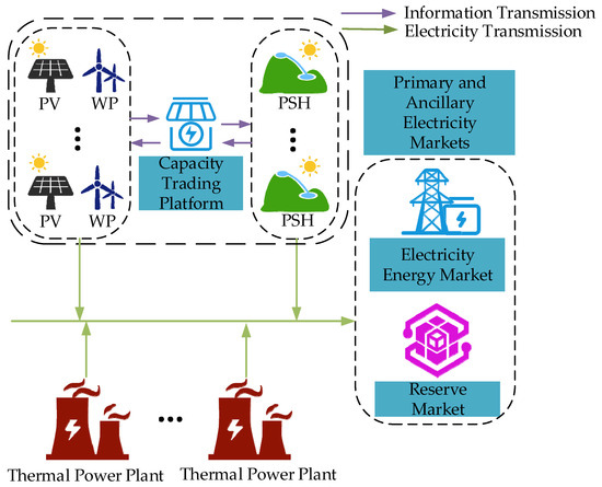
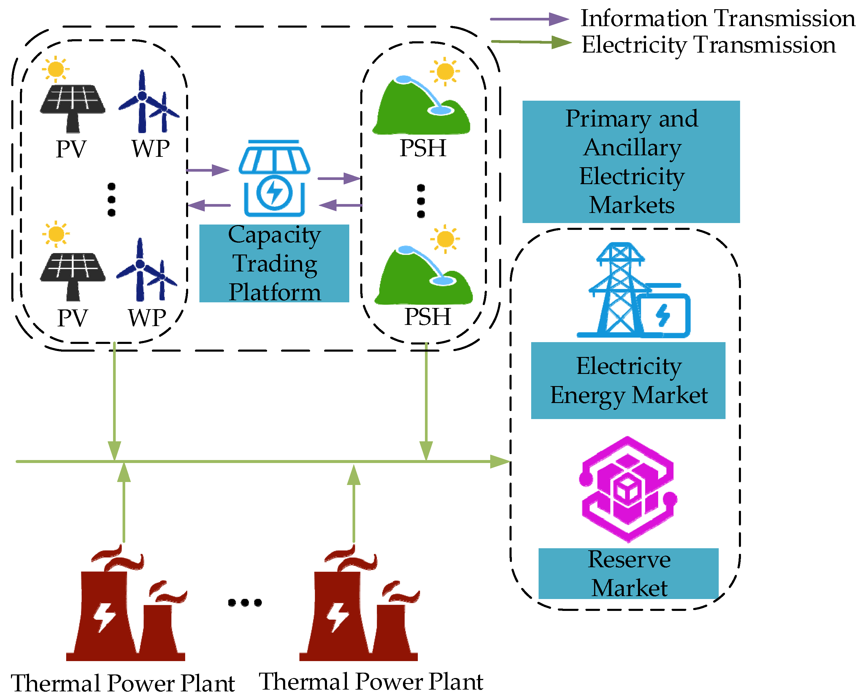
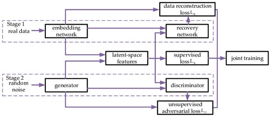
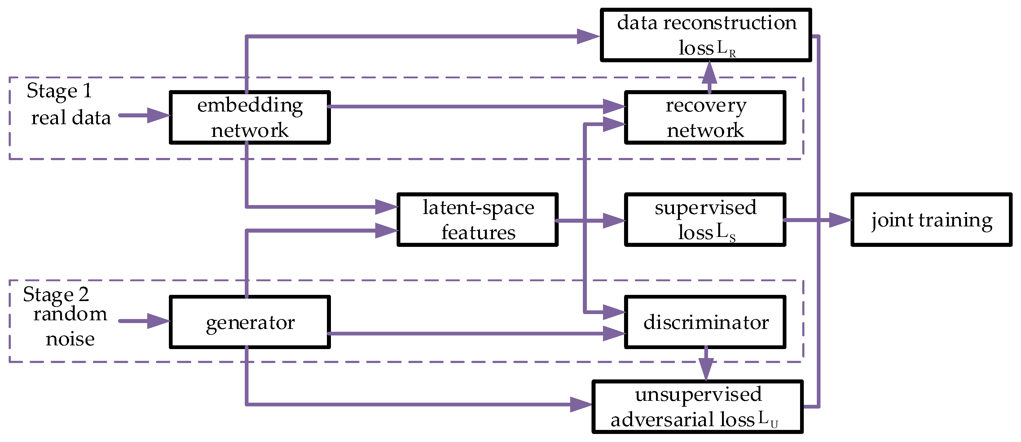
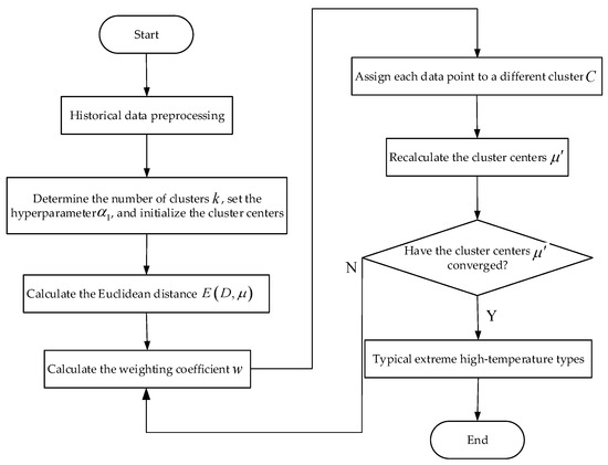
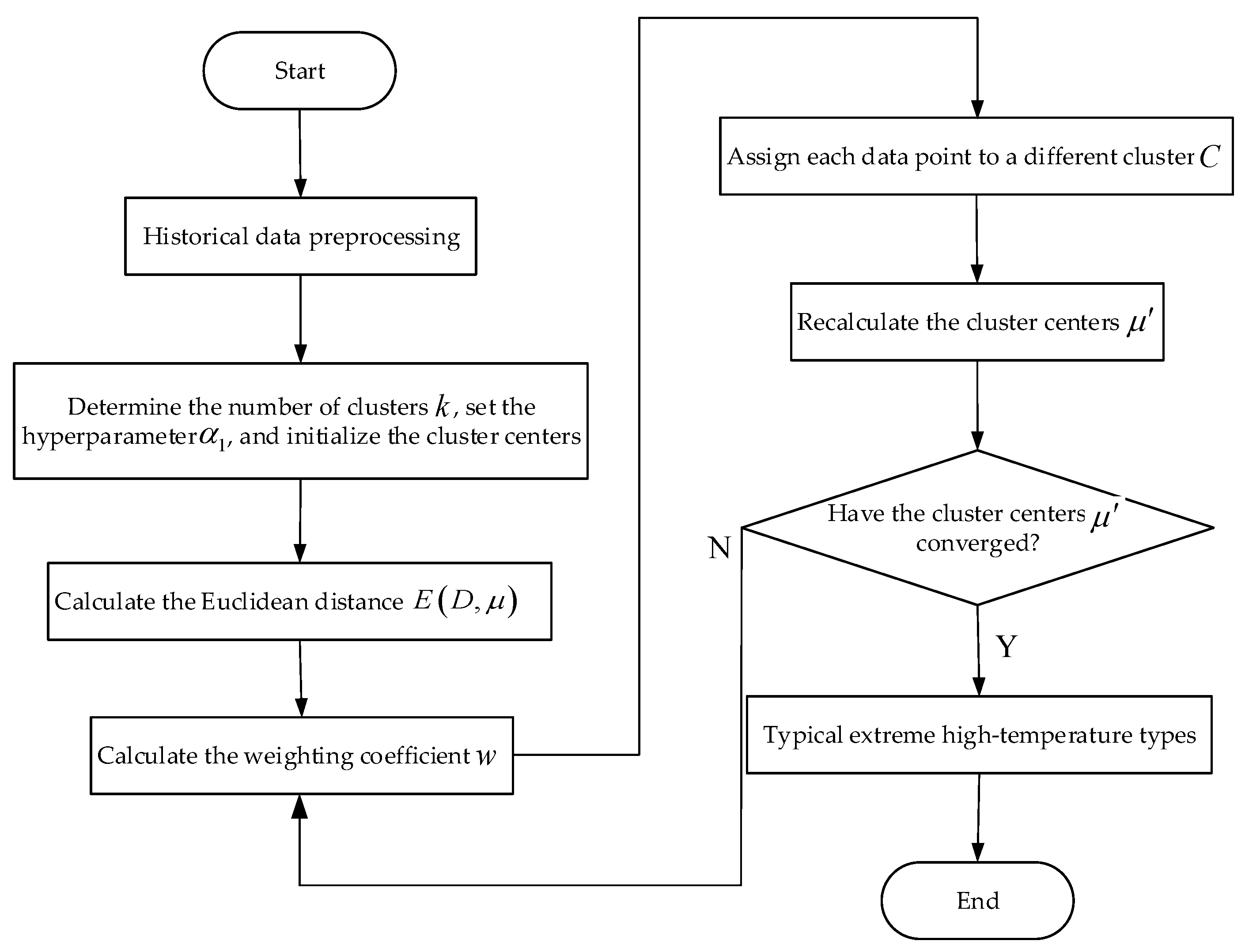
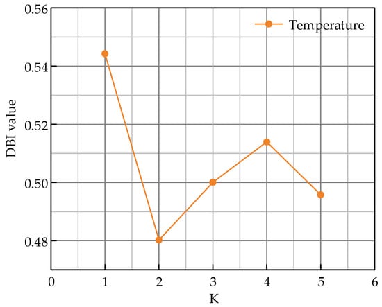
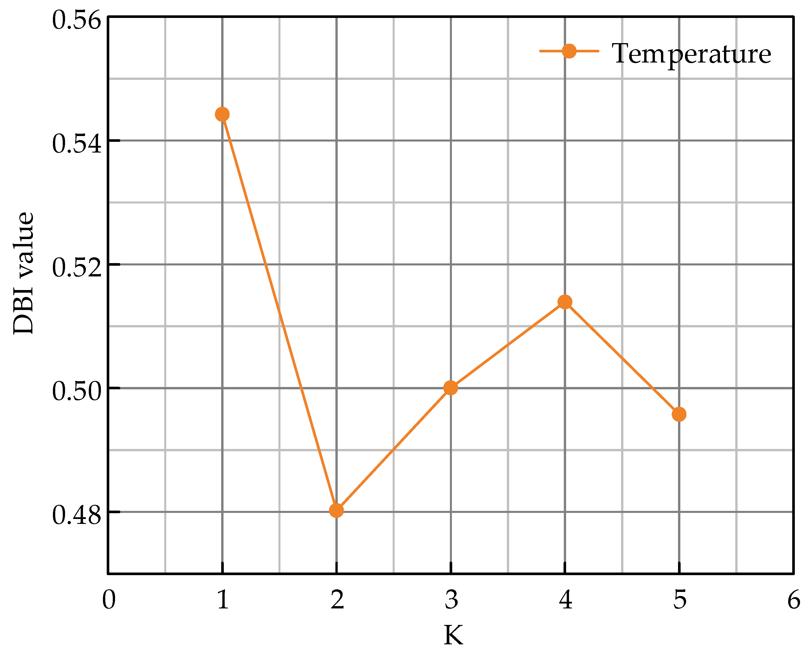
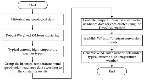
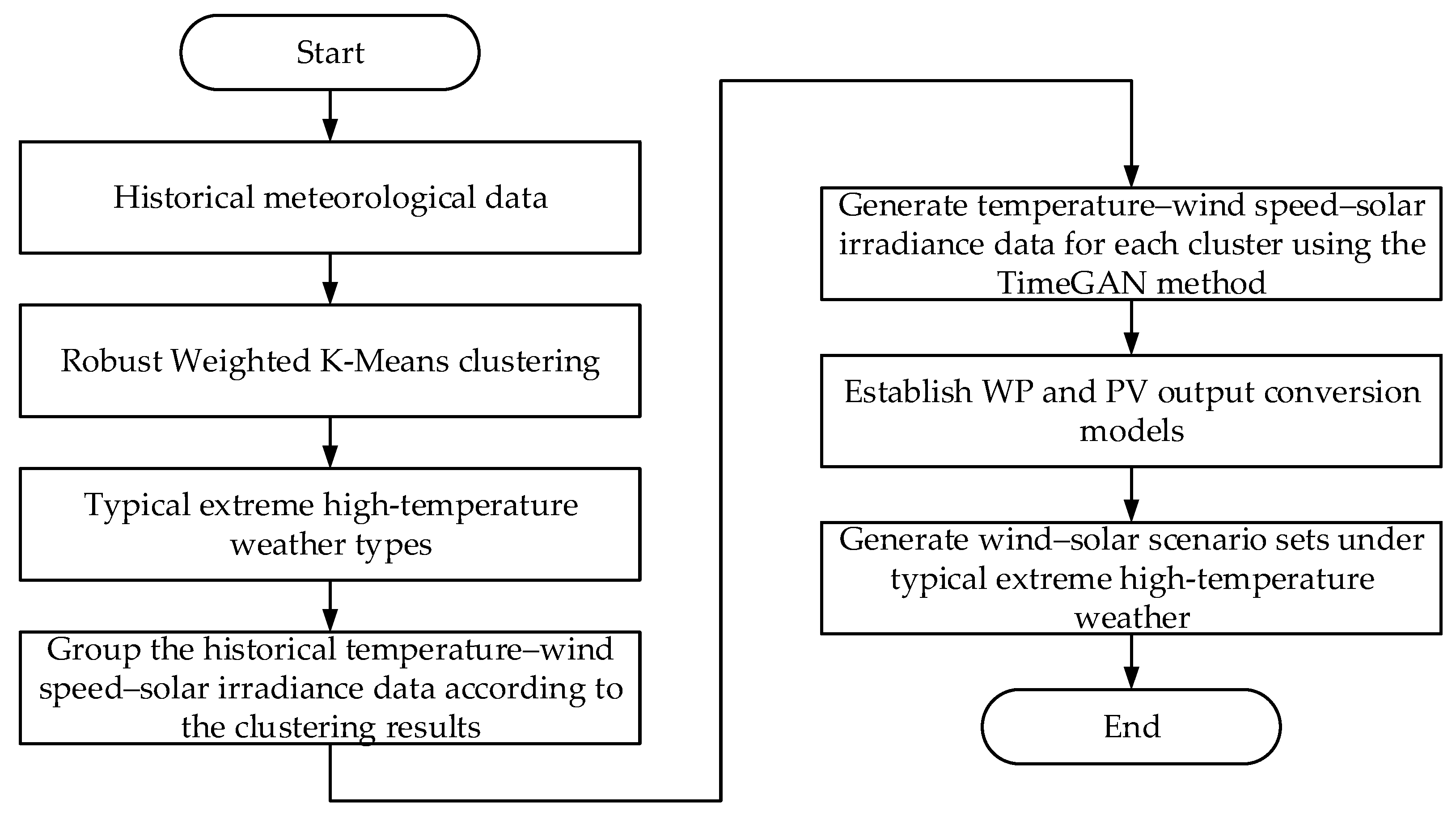
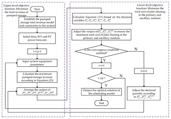
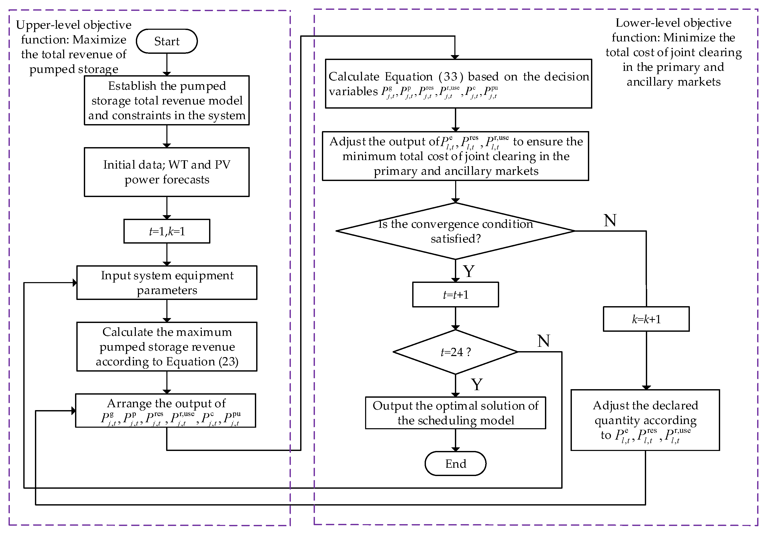
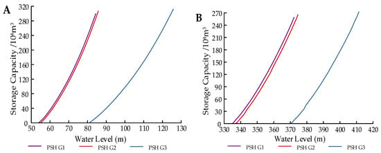
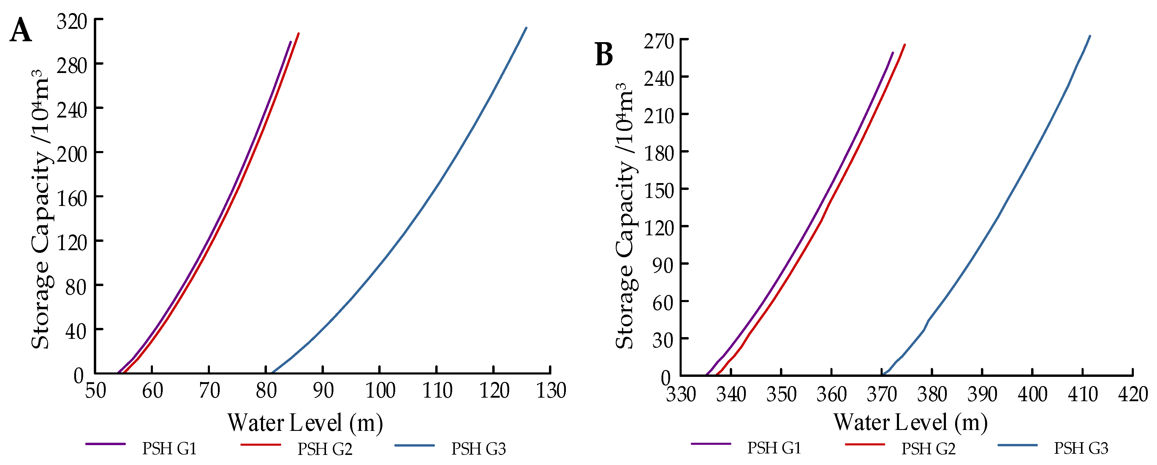
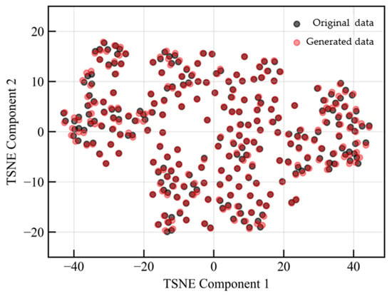
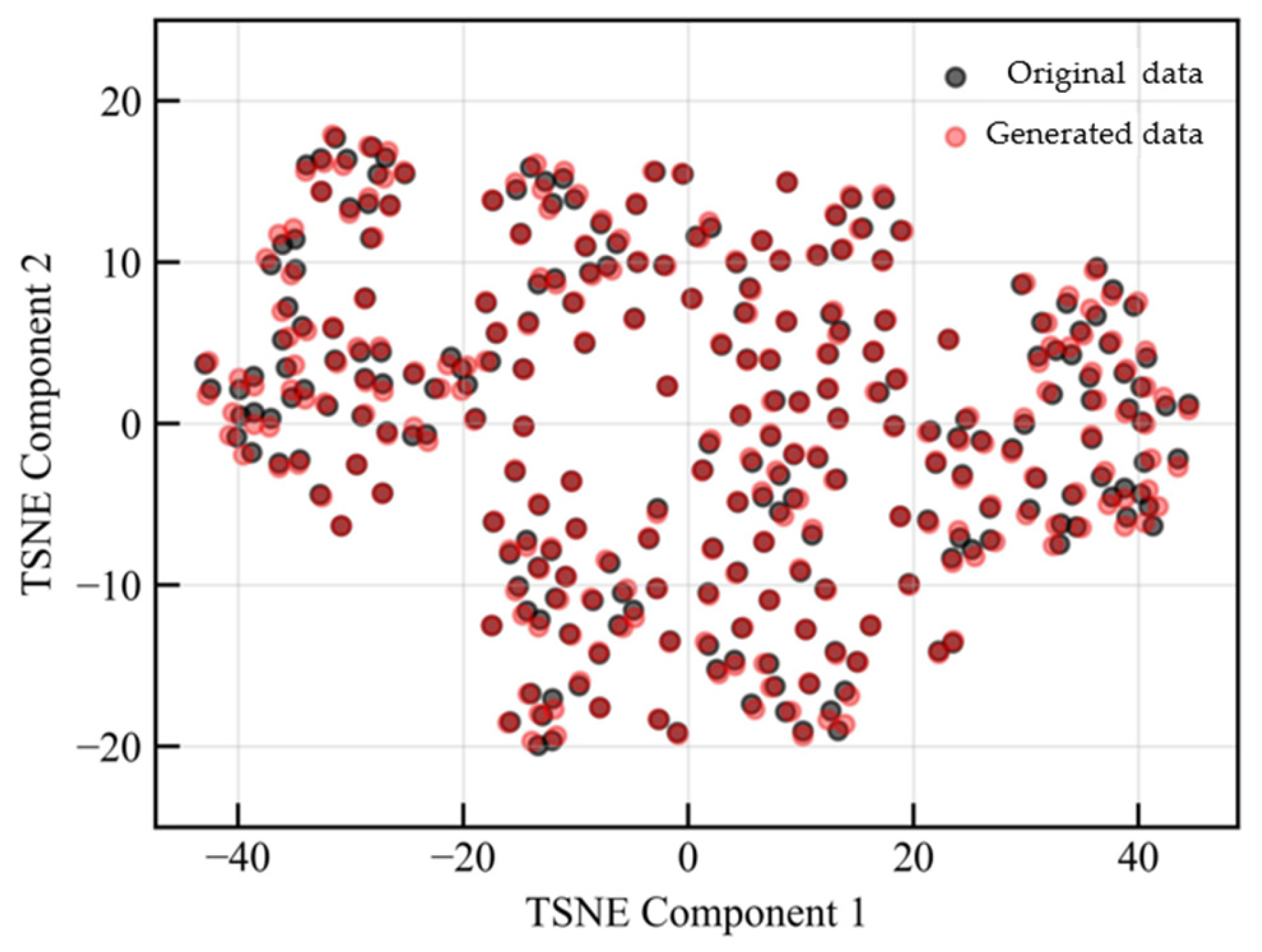
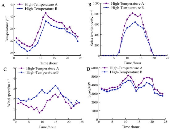
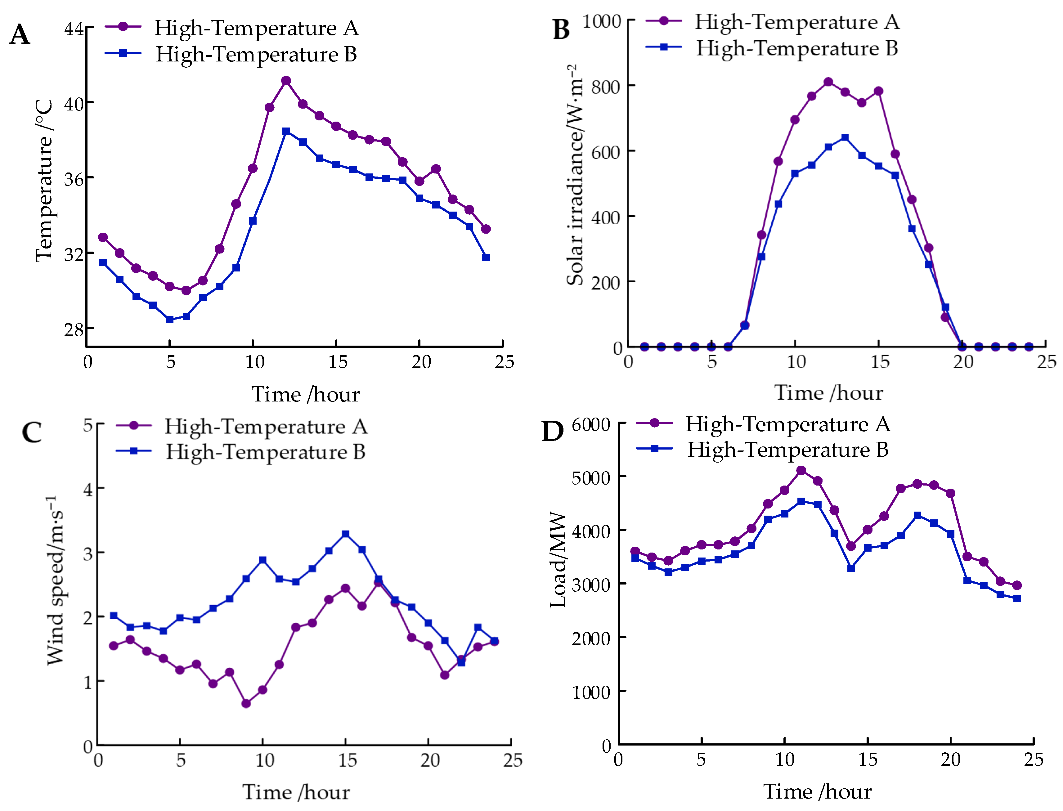
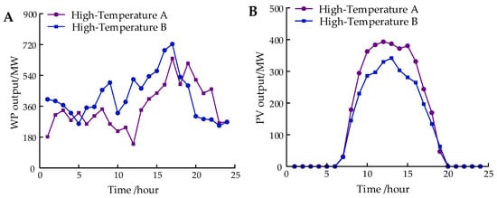
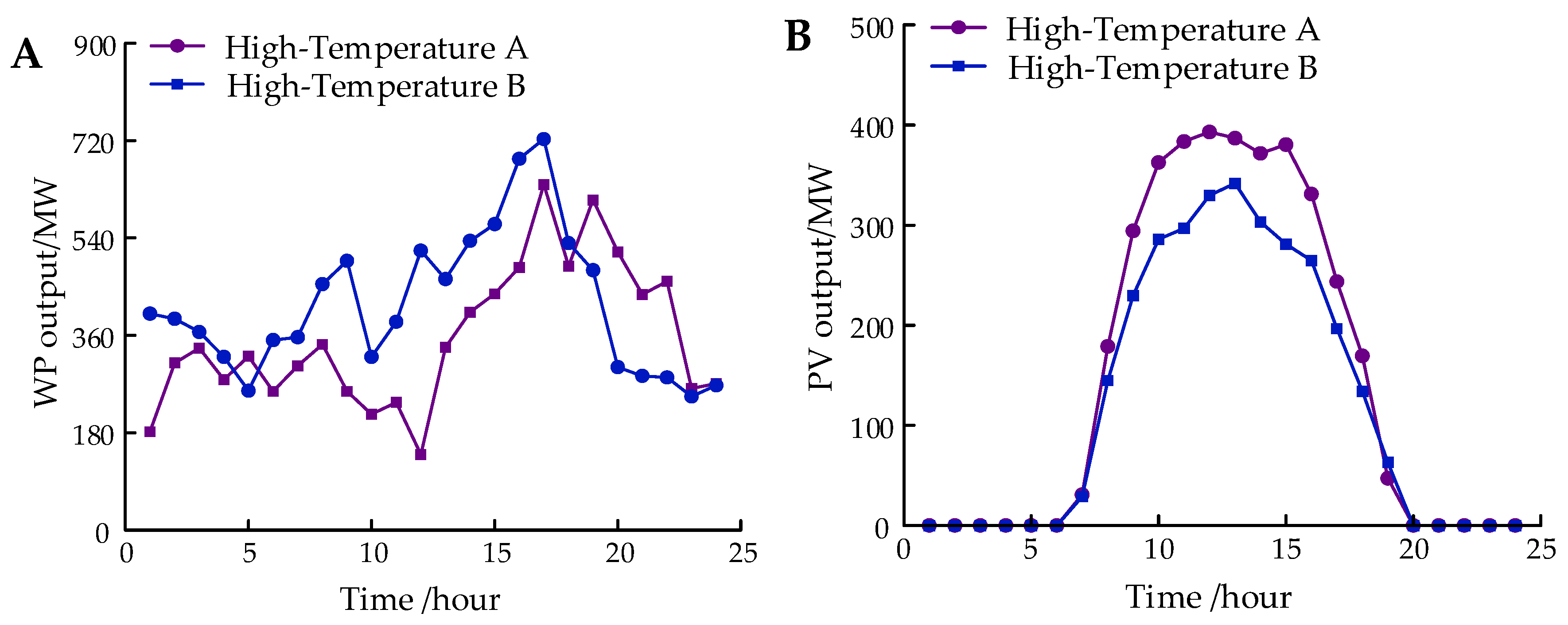
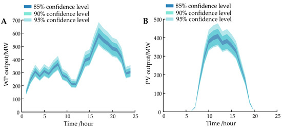
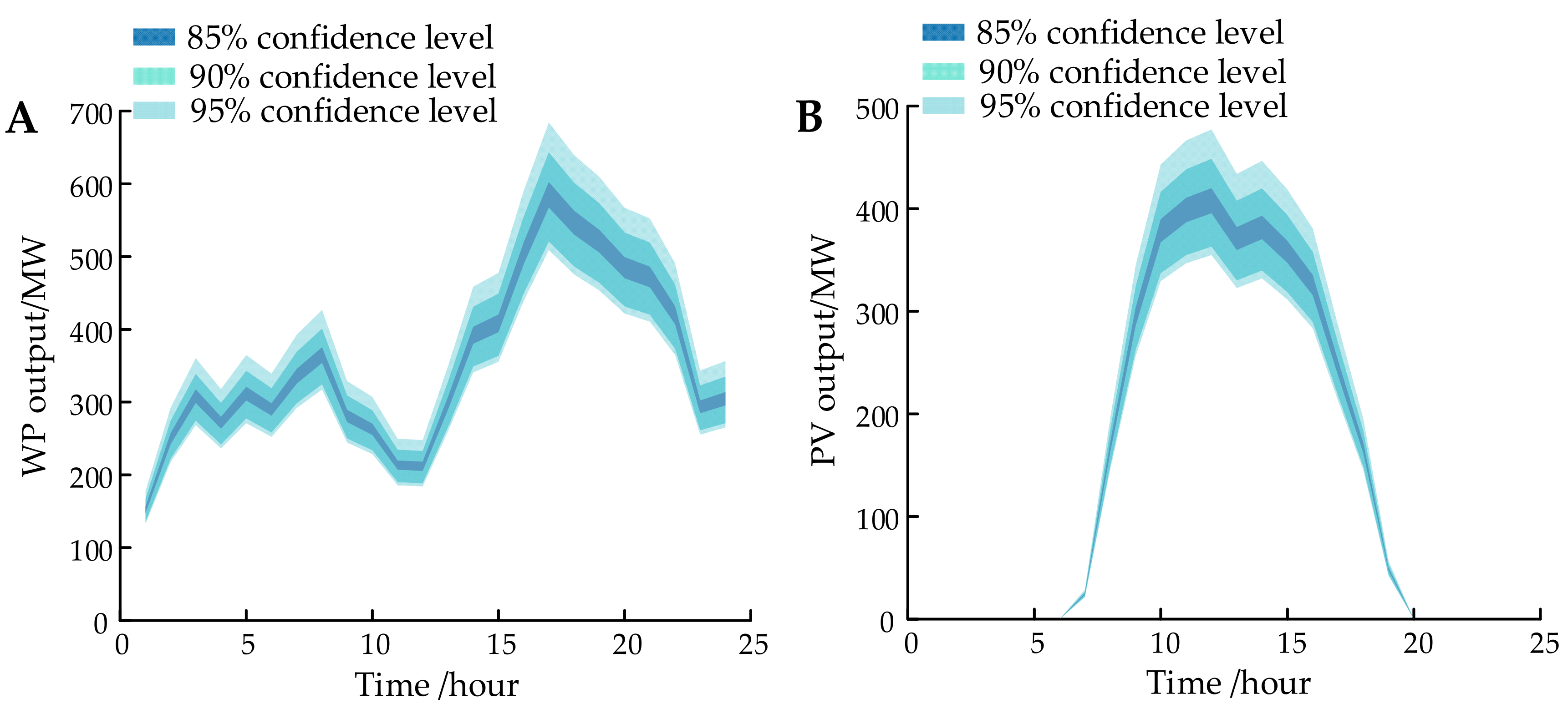
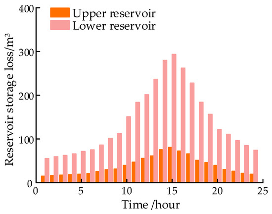
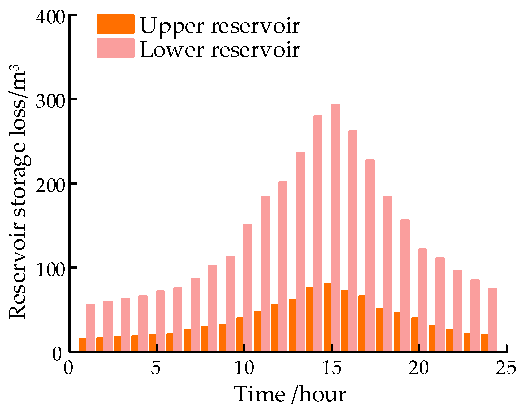
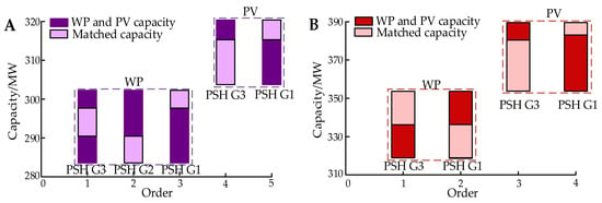
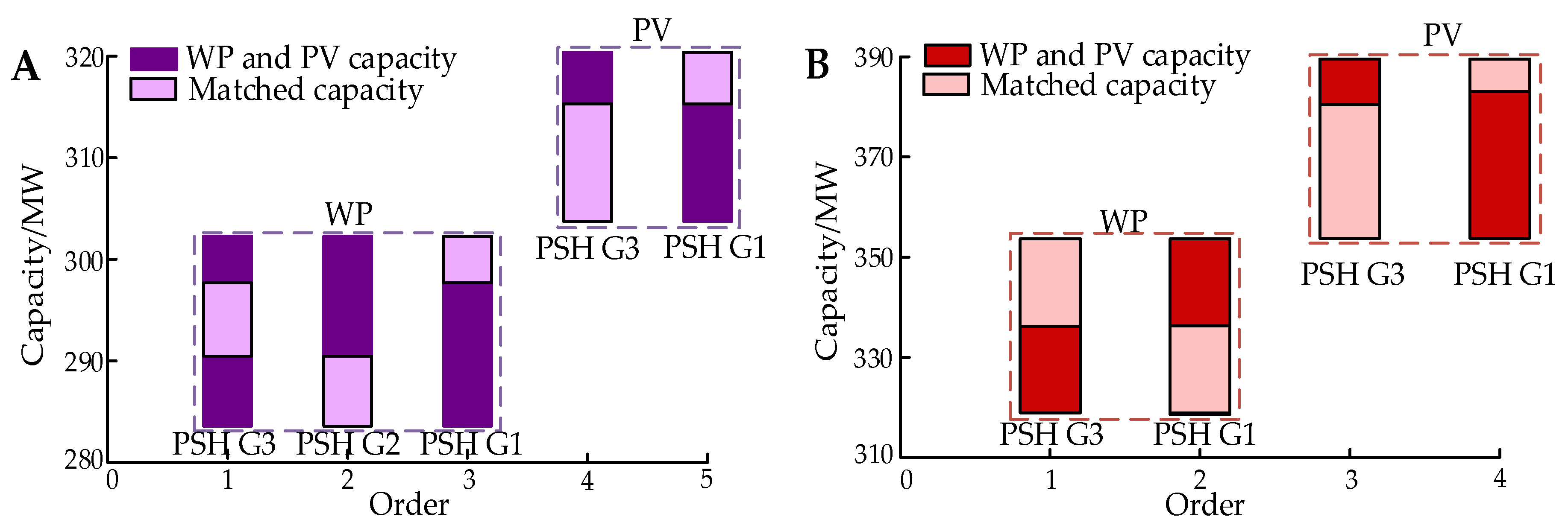
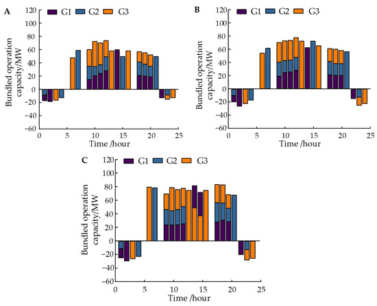
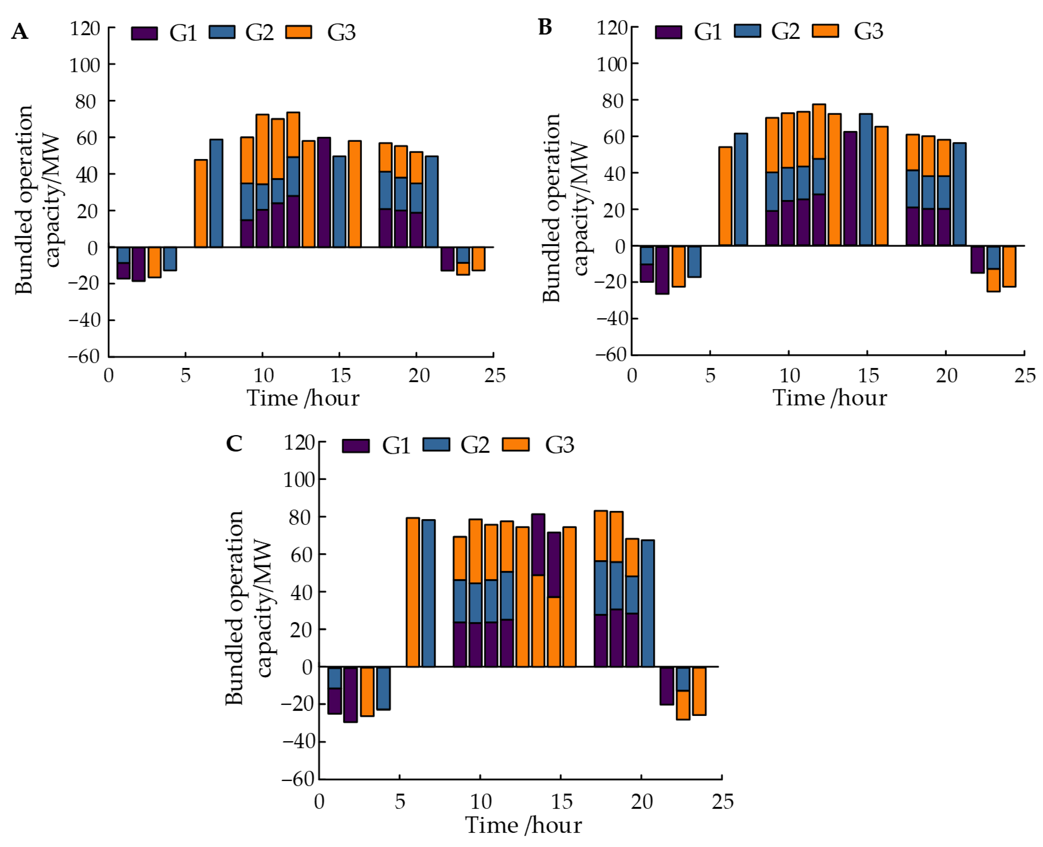
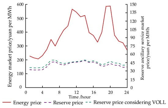
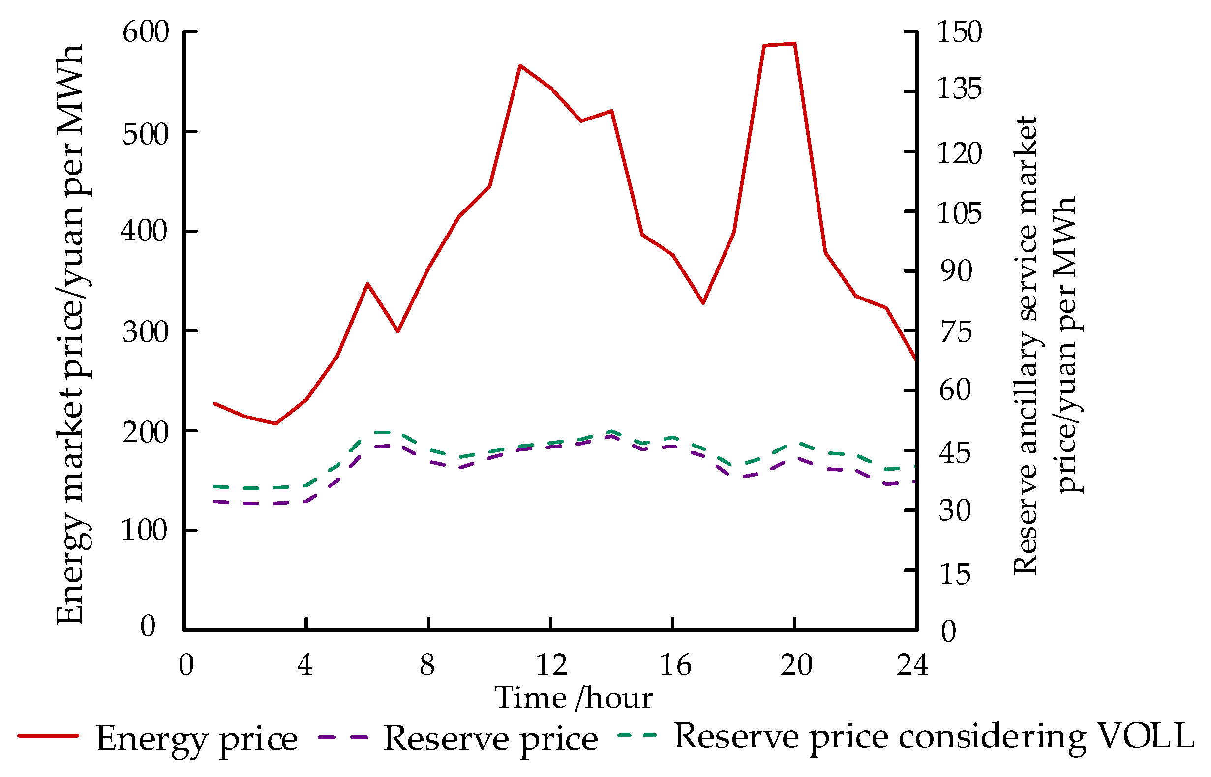
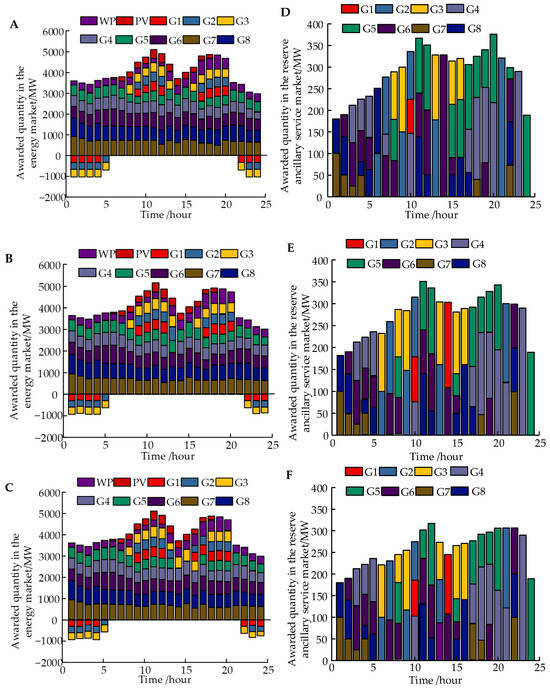
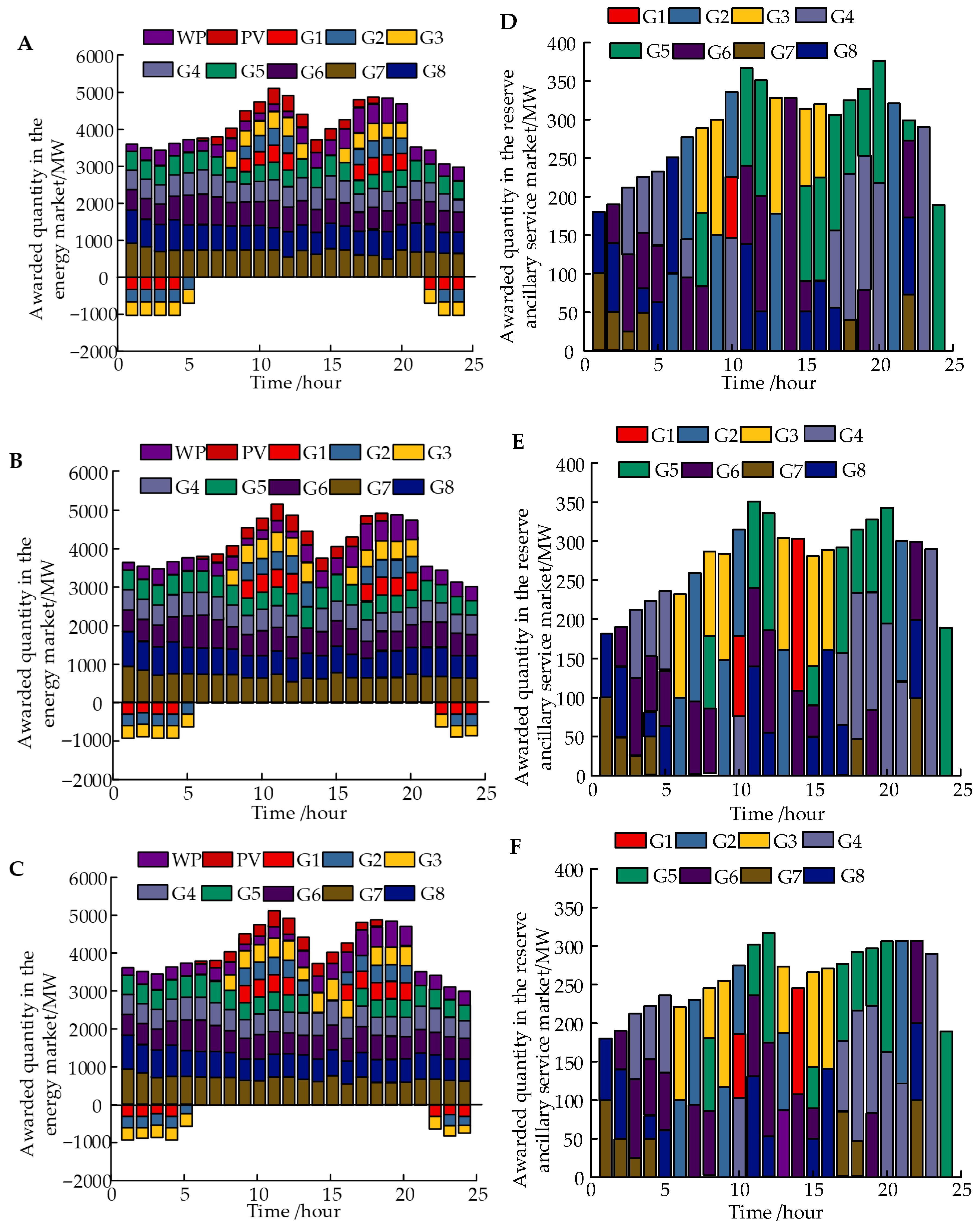

Disclaimer/Publisher’s Note: The statements, opinions and data contained in all publications are solely those of the individual author(s) and contributor(s) and not of MDPI and/or the editor(s). MDPI and/or the editor(s) disclaim responsibility for any injury to people or property resulting from any ideas, methods, instructions or products referred to in the content. |
© 2026 by the authors. Licensee MDPI, Basel, Switzerland. This article is an open access article distributed under the terms and conditions of the Creative Commons Attribution (CC BY) license.