A Simplified and Automated Building Energy Retrofit Analysis Approach

Abstract

Retrofitting existing buildings is widely recognized as a critical strategy for achieving global decarbonization goals. As a part of this effort, several tools have been developed for building retrofit analysis, each offering distinct advantages and limitations. However, the current approaches and tools still lack the capability to generate well-calibrated detailed building energy models that can evaluate both individual and combined energy efficiency measures. Moreover, no existing analysis tool can identify the most cost-optimal combination of retrofit measures through a comprehensive optimization search using different objectives. To address these shortcomings, this paper describes a new Simplified and Automated Building Energy Retrofit (SABER) analysis approach and tool. The SABER tool is a Python-based interactive platform designed to assist users by automatically creating detailed energy models of existing buildings. It incorporates a novel automatic calibration algorithm that adjusts operational schedules using building energy signature characteristics, ensuring accurate model performance. In addition, SABER can assess various building energy efficiency measures using a sequential search technique to determine the most cost-effective retrofit packages. This paper describes the key functionalities of SABER and demonstrates its capabilities through two residential building case studies. By integrating several key features into a unified framework, SABER represents a significant step toward the next generation of building energy retrofit analysis tools that can effectively assist the industry’s transition to a sustainable future.

1. Introduction

Globally, existing buildings account for close to 80% of the entire building stock [1]. Consequently, retrofitting existing buildings is one of the key strategies for achieving our climate goals [2]. Several studies have evaluated the potential energy savings associated with implementing retrofit measures. For instance, a study of the residential sector in Italy determined that a nearly 24.8% reduction in energy was possible through envelope retrofits alone [3]. In the US, a review of buildings participating in the Energize Phoenix program showed energy saving potentials of 12% for commercial buildings and 8% for residential buildings were associated with the deployment of retrofit measures [4]. Similarly, an early measurement and verification (M&V) study estimated median electricity savings of about 16% in annual energy consumption using pre- and post-retrofit utility data from single-family residential buildings [5]. Further, another review of 39 residential buildings’ retrofit projects estimated an average reduction in measured fuel consumption of 7.2% [6].

Despite the well-documented benefits, the rate of deep energy retrofits of existing buildings remains at less than 1% of the existing building stock per year [7]. However, to achieve complete decarbonization by 2050, an annual deployment rate of over 2% is needed [8]. Studies show financial considerations as the primary obstacle for the implementation of retrofit measures in residential buildings [9]. Energy retrofit projects are traditionally associated with high capital investments, high payback periods, and a magnitude of hidden management and labor costs [10]. Additionally, the lack of technical expertise and domain knowledge among homeowners and building managers has also proven to be a major roadblock in both the evaluation and implementation of energy efficiency renovations [11]. To alleviate some of these barriers, several retrofit strategies and decision tools have been developed [12].

Potential energy efficiency measures are typically identified through periodic and systematic energy audits. The American Society of Heating, Refrigerating, and Air-Conditioning Engineers (ASHRAE) details the procedures to conduct a successful energy audit in the ASHRAE Standard 211 [13]. Depending on the available resources, timeframe, budgets, building complexity, and client’s requirements, the ASHRAE classifies energy audits for buildings into three levels: (1) Level 1 is based on a walk-through assessment, (2) Level 2 uses an energy survey and analysis, and (3) Level 3 requires a detailed analysis of capital-intensive modifications. To determine accurate energy and cost savings from the selected retrofit measures, energy audits, especially those based on Level 3 analyses, are often augmented by developing calibrated models using whole-building energy simulation tools, such as EnergyPlus [14] and DOE2.2 [15]. However, the use of such detailed whole-building energy analysis tools significantly increases the effort and time required to make effective building retrofit decisions. Indeed, developing calibrated energy models for existing buildings can be both complex and time intensive [16]. Consequently, this challenge necessitates the adoption of rapid assessment strategies that can simplify the decision-making process while maintaining sufficient accuracy.

A wide variety of interactive tools have been developed to facilitate and aid energy auditing of commercial and residential buildings. Detailed reviews of existing tools suitable for energy audits of buildings have been reported by Gonzalez-Caceres et al. [11], Seddiki et al. [12], Lee et al. [17], and Forouzandeh et al. [18], using a series of different criteria for tool selection. The reviews by Gonzalez-Caceres et al. [11] and Seddiki et al. [12] focused on energy assessment tools applicable exclusively to residential buildings, while those by Lee et al. [17] and Forouzandeh et al. [18] covered tools suitable for both commercial and residential buildings. Based on these reviews, more than thirty different tools have been identified as suitable for the purpose of aiding in building energy retrofit decisions. Typically, these tools provide a user-friendly interface for easy visualization of input and output data and utilize sets of algorithms to evaluate the energy performance of existing buildings [17]. In addition, Lee et al. [17] classified the existing tools into three categories according to their underlying modeling paradigm: (a) empirical data-driven methods that rely on measured utility/smart meter data and black-box models, (b) reduced order modeling using simple Resistor–Capacitance (RC) network models with a given structure and normative model parameters, and (c) detailed whole-building energy simulation models. In this paper, a flexible retrofit analysis approach is introduced to combine data-driven and physics-based models with optimized selection of energy efficiency measures for existing buildings.

Several of the identified retrofit analysis tools utilize one or multiple benchmarking strategies to evaluate the cost and energy implications of different retrofit measures. The benchmarking methods predominantly fall into three categories: (a) benchmarking against a user-given portfolio of buildings of similar type and climate [19], (b) benchmarking against predefined national databases of buildings of same type and climate [19,20] and, (c) benchmarking against the potential performance of a building predicted from white-box simulation models [21,22,23].

This paper focuses on the tools that fall into the third category, i.e., those capable of performing detailed building energy simulations. Table 1 lists some of the tools that fall into this category based on the previously mentioned reviews. Most of the tools listed in Table 1 utilize EnergyPlus as the underlying simulation engine. By conducting whole-building energy simulations, these tools can evaluate and compare the energy and cost benefits of several measure packages. However, not all tools calibrate the building energy models with the utility data, as indicated by the calibration column in Table 1. Prior research has shown that calibrating or matching the results of building energy models with the utility data is critical to evaluating energy efficiency measures accurately [24].

Table 1. Main features of a few open-source tools that can be used for retrofit analysis using whole-building energy simulation models gathered from the existing literature.

Tool	Simulation Engine	Calibration	Measures Package Analysis	Hosted/Developed By	Region	Reference
Commercial Building Energy Asset Scoring Tool	EnergyPlus	No	Yes	US DOE	US	[22]
MulTEA	DOE2.2	Yes	Yes	ONRL	US	[25]
Buildbee (previously known as Simuwatt)	EnergyPlus	Yes	Yes	NREL	US	[26,27]
California Building Energy Code Compliance Software	EnergyPlus	No	Yes	NORESCO	California	[28]
Commercial Building Energy Saver	EnergyPlus	Yes	Yes	LBNL	California	[23]
HOT2XP	HOT2000	Yes	Yes	CAMNET Energy Technology Center, NRCan	Canada	[29,30]
BEOpt	EnergyPlus	No	Yes	NREL	US	[31]
CityBES	EnergyPlus	Yes	Yes	LBNL	US	[32]
XeroHome	EnergyPlus	No	Yes	NREL	Some regions of US	[33]

While many tools claim to perform some form of calibration, their underlying algorithms are often not clearly documented. For example, MulTEA [25] and BuildBee [26] indicate that model calibration is performed, yet the specific methods are not described. In several cases, the building energy model calibration process merely refers to evaluating the error between the simulated and measured energy use. However, error evaluation alone is insufficient to ensure predictive accuracy of detailed building energy models. To achieve credible retrofit analysis results, careful adjustment of input parameters to minimize discrepancies is essential [24].

Among the surveyed tools, the Commercial Building Energy Saver (CBES) [23] provides the most transparent and well-documented description of the calibration method used for detailed energy models of existing buildings. The CBES employs a pattern-based approach to identify both universal and seasonal deviations between the simulation results and utility data. It then systematically adjusts the key input parameters, such as occupant density, lighting and equipment power density, HVAC efficiencies, and wall constructions, etc., to eliminate model discrepancies. Although this approach effectively corrects model predictions, it relies on the uncertainty of input parameters for the building energy models. When all input parameters are well known, the benefits of the proposed calibration approach are lost and, conversely, when too many input parameters are unknown, the calibration problem becomes too complex and computationally intractable to solve.

A wide array of retrofit approaches and tools exist that allow users to evaluate building performance with minimum input data and limited expertise requirements. However, the reported literature continues to highlight significant shortcomings in the existing toolkits, specifically the following:

• Many of the available tools still lack the ability to let users select and evaluate specific energy retrofit measures. Moreover, the available tools provide retrofit recommendations based on a pre-specified set of energy efficiency options and established best practices [12,17]. However, the literature reports that allowing users to evaluate specific energy retrofit measures based on their energy and cost impacts and their practical feasibility enhances their sense of support during the energy audit process [34]. This increased satisfaction can lead to an increased likelihood of actual implementation of the recommended measures.
• Studies have shown that performance of an individual retrofit measure applied to an existing building can differ significantly from the performance of an integrated retrofit package [35]. Only 20% of more than forty reviewed tools are based on analyses using detailed building energy models. The lack of detailed modeling approaches in several of the existing toolkits makes it challenging to determine the interactive effects of energy and cost benefits among multiple selected measures required for evaluating optimal retrofit packages [12,17].
• Large discrepancies between the predicted energy performance of developed building energy models and the actual metered data can result in overestimation of energy savings and underperformance of retrofit measures. These discrepancies can be attributed to (1) variability in occupant behaviors, (2) impact of climatic conditions, (3) changes in operation and maintenance settings, (4) variations in indoor environmental conditions, (5) inaccurate modeling of internal heat gains, and (6) use of incorrect input parameters for building energy models. To limit these prediction inaccuracies, building energy models need to be calibrated [24]. Of the evaluated toolkits, only one provides a well-documented description of the corresponding model calibration methodology.
• Current retrofit toolkits lack the capability to identify the optimal combination of energy efficiency measures, instead relying on users’ judgments. As the number of potential retrofit measures increases, the search process becomes computationally intensive due to the large solution space and repeated input/output processing. While computerized option analysis can automate these tasks, the number of required simulations remains significant, requiring substantial computational efforts. To improve efficiency, optimal search techniques [36] need to be utilized to decrease the number of simulations required to identify the best package in comparison to a full factorial search of all possible combinations.
• Finally, many of the reviewed tools are hosted on outdated or unsupported websites, lack comprehensive technical documentation, and require a substantial learning curve to access and use effectively.

While some of the available tools can overcome one or more of these limitations, no approach is currently able to provide a comprehensive platform that integrates all the noted functionalities. Doing so would provide users with a unified solution that could be used to aid in the retrofitting of existing buildings. To this end, this paper introduces the Simplified and Automated Building Energy Retrofit (SABER) analysis approach, deployed in a user-friendly tool. SABER is an EnergyPlus-based interactive tool that can be used to generate calibrated energy models of existing buildings and identify the optimal retrofit opportunities. A general description of all the key functionalities of SABER is provided in the first section of the paper. Subsequently, each functionality is described in detail and, finally, some of the capabilities are illustrated using two different existing building case studies.

2. Introduction to the Simplified and Automated Building Energy Retrofit (SABER) Analysis Tool

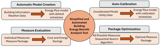
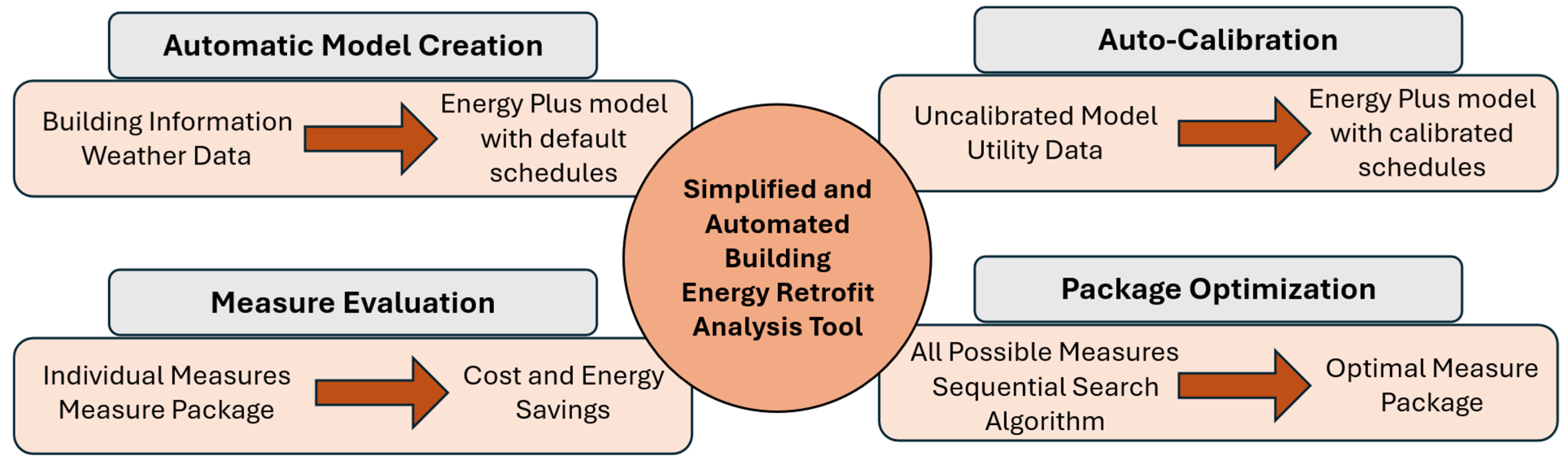
SABER is a Python-based tool with an interactive graphic user interface that creates a platform for the user to model and analyze individual, combined, and optimized retrofit options for existing buildings. SABER utilizes basic user input information to generate a detailed whole-building energy simulation model of the existing building based on predefined model templates. The developed initial building energy model is then calibrated based on the utility data collected as part of the user input phase. SABER requires at least one year (i.e., 12 months) of utility data to ensure proper calibration of the generated energy model, while data from multiple years is averaged into energy usage of one representative year. The calibrated building energy model is then used to accurately assess the impact of both individual and packaged energy efficiency measures. SABER is equipped to handle energy and cost interactions among multiple retrofit measures, whether selected manually by the user or through an optimization search defined by a desired objective function and a set of constraints. Figure 1 outlines the main functions and current capabilities of the SABER analysis tool. The current version of SABER tool can be accessed in the link provided in the Supplementary Materials section.

Figure 1. An overview of all functionalities of the Simplified and Automated Building Energy Retrofit (SABER) analysis tool.

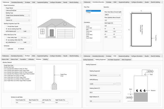
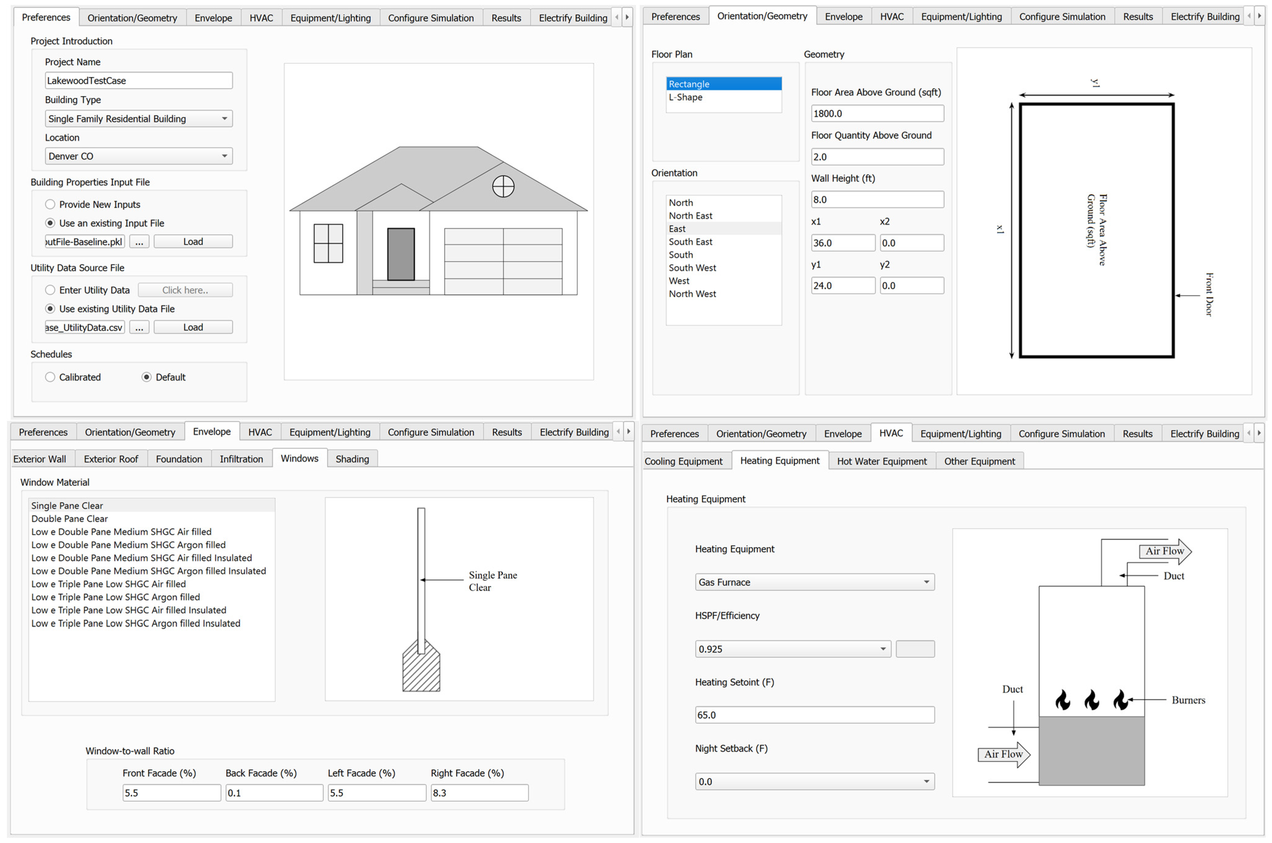
As shown in Figure 1, the four main functionalities of SABER tool include (1) the automatic generation of building energy model suitable for EnergyPlus using the user-specified input data, (2) an automatic calibration algorithm to match the simulation predictions with the utility data, (3) an evaluation module to estimate cost and energy savings of individual and packaged energy efficiency measures, and (4) an optimization module to identify the most cost-effective combination of retrofit measures based on the user-selected cost functions and constraints. The following sections describe each of these functionalities in greater detail. Figure 2 shows a few input screens from the performance of a retrofit analysis using SABER.

Figure 2. Sample SABER screens for inputting building information for a chosen case study.

3. Automatic Model Creation Methodology

To streamline the process of generating a whole-building energy simulation model, SABER relies on information provided by the user using a few input screens with different built-in options, as illustrated in Figure 2 [31]. Table 2 shows the list of the possible options available currently for each input parameter using SABER Version 1.0.

Table 2. Table of different input options available in SABER.

Property	Possible Options
Geometry Shape	Rectangle L-shape
Orientation	North, northeast, east, southeast, south, southwest, west, northwest
Building Shape Parameters	Area, floor quantity, wall height, length, breadth
Exterior Wall Construction	2 × 4 insulated wood studs with vinyl siding 2 × 4 insulated wood studs with brick finish Insulated 8 in. concrete
Wall Insulation	Uninsulated, R7, R11, R13, R15, R19, R23, R36
Roof Construction	Asphalt shingles
Attic Insulation	Uninsulated, R7, R11, R13, R19, R30, R49, R60
Foundation	Slab-on-grade Crawlspace Unconditioned basement
Infiltration Level	25 ACH50–2 ACH50
Window Material	Single pane, clear (5.67 W/m2K U-value, 0.76 SHGC) Double pane, clear (2.78 W/m2K U-value, 0.56 SHGC) Low-e double pane, medium SHGC, air filled (2.10 W/m2K U-value, 0.3 SHGC) Low-e double pane, medium SHGC, argon filled (1.98 W/m2K U-value, 0.44 SHGC) Low-e double pane, medium SHGC, air filled, insulated (1.70 W/m2K U-value, 0.46 SHGC) Low-e double pane, medium SHGC, argon filled, insulated (1.53 W/m2K U-value, 0.46 SHGC) Low-e triple pane, low SHGC, air filled (1.64 W/m2K U-value, 0.26 SHGC) Low-e triple pane, low SHGC, argon filled (1.53 W/m2K U-value, 0.26 SHGC) Low-e triple pane, low SHGC, air filled, insulated (1.07 W/m2K U-value, 0.27 SHGC) Low-e triple pane, low SHGC, argon filled, insulated (0.96 W/m2K U-value, 0.27 SHGC)
Window-to-Wall Ratio	Front, back, left, right
Window Parameters	Average window height Average number of windows per wall Overhang depth
Cooling Equipment	Air conditioner Air source heat pump
Heating Equipment	Gas furnace Electric furnace Air source heat pump
HVAC Controls	Heating and cooling setpoint, night setback
Domestic Hot Water System	Gas boiler Electric boiler
DHW Capacity	DHW tank volume
Electric Equipment	Cooking range Dishwasher Clothes washer Clothes dryer Refrigerator Microwave Office Eqp. (computers, printers, etc.) Miscellaneous plug loads

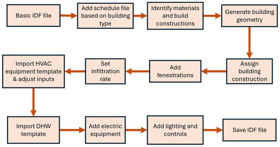
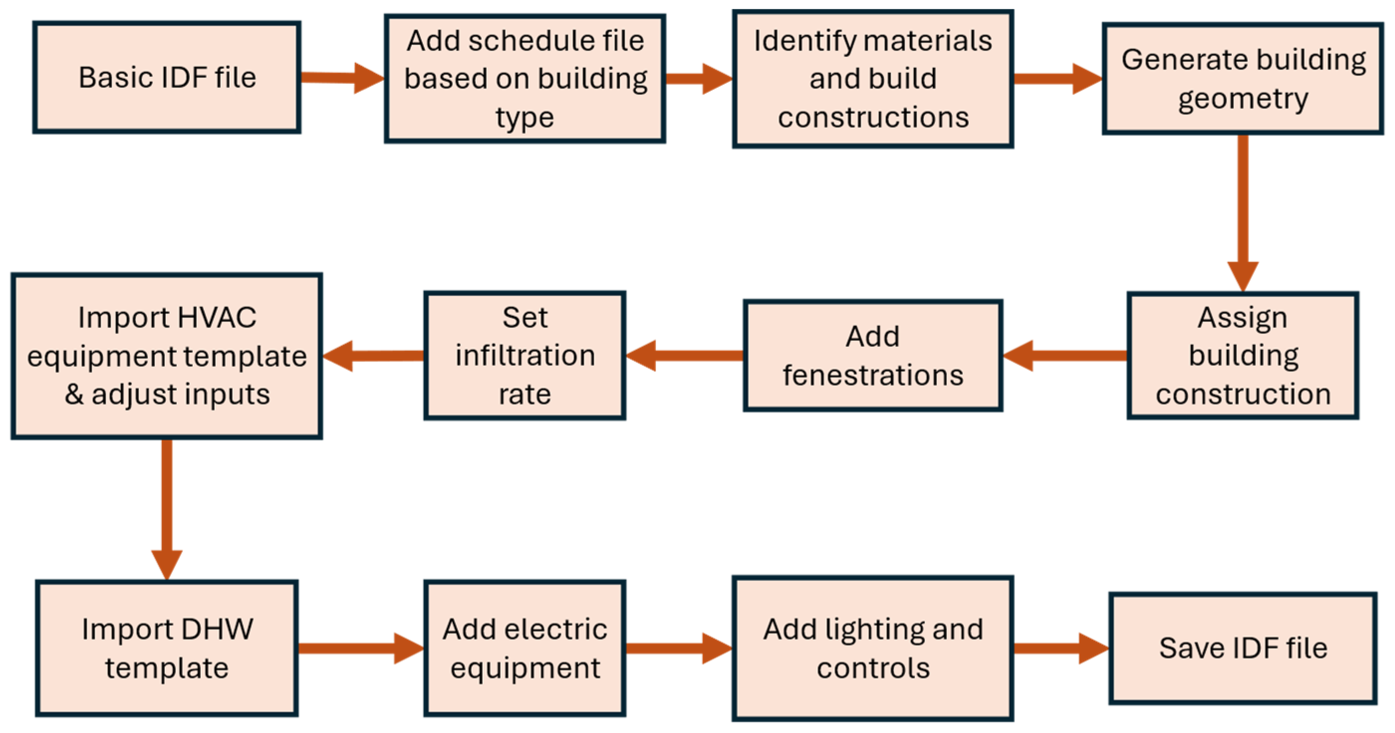
As depicted in Figure 3, a simplified automatic approach is used to develop an energy model suitable for conducting a detailed whole-building energy analysis using EnergyPlus Version 22.2 [14]. First, a pre-specified generic EnergyPlus Input Data File (IDF) template is used to import some basic simulation parameters. This generic IDF template is adjusted to account for the user-defined building type to identify the appropriate building operation schedules, including typical occupancy profiles and lighting and equipment usages, based on established prototypical building energy models [31]. Then, the specifications for the building geometry, surface constructions, fenestration specifications, air infiltration rates, HVAC systems, domestic water heaters, appliances, and lighting systems are added based on the user-provided information collected through the SABER input screens in the order illustrated in Figure 3.

Figure 3. Flowchart showing steps used to generate EnergyPlus Input Data File (IDF) in SABER.

The IDF descriptions of the user-selected HVAC and domestic hot water systems are imported using pre-existing templates, included as part of SABER. Based on the building location, the closest available weather data for a Typical Meteorological Year (TMY3) is queried using an EnergyPlus Weather (EPW) file. The final building-specific IDF file generated by this module, along with the corresponding tool inputs, is saved in the project directory and used to execute a primary energy simulation of the building.

4. Automatic Calibration of Building Energy Model

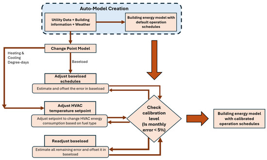
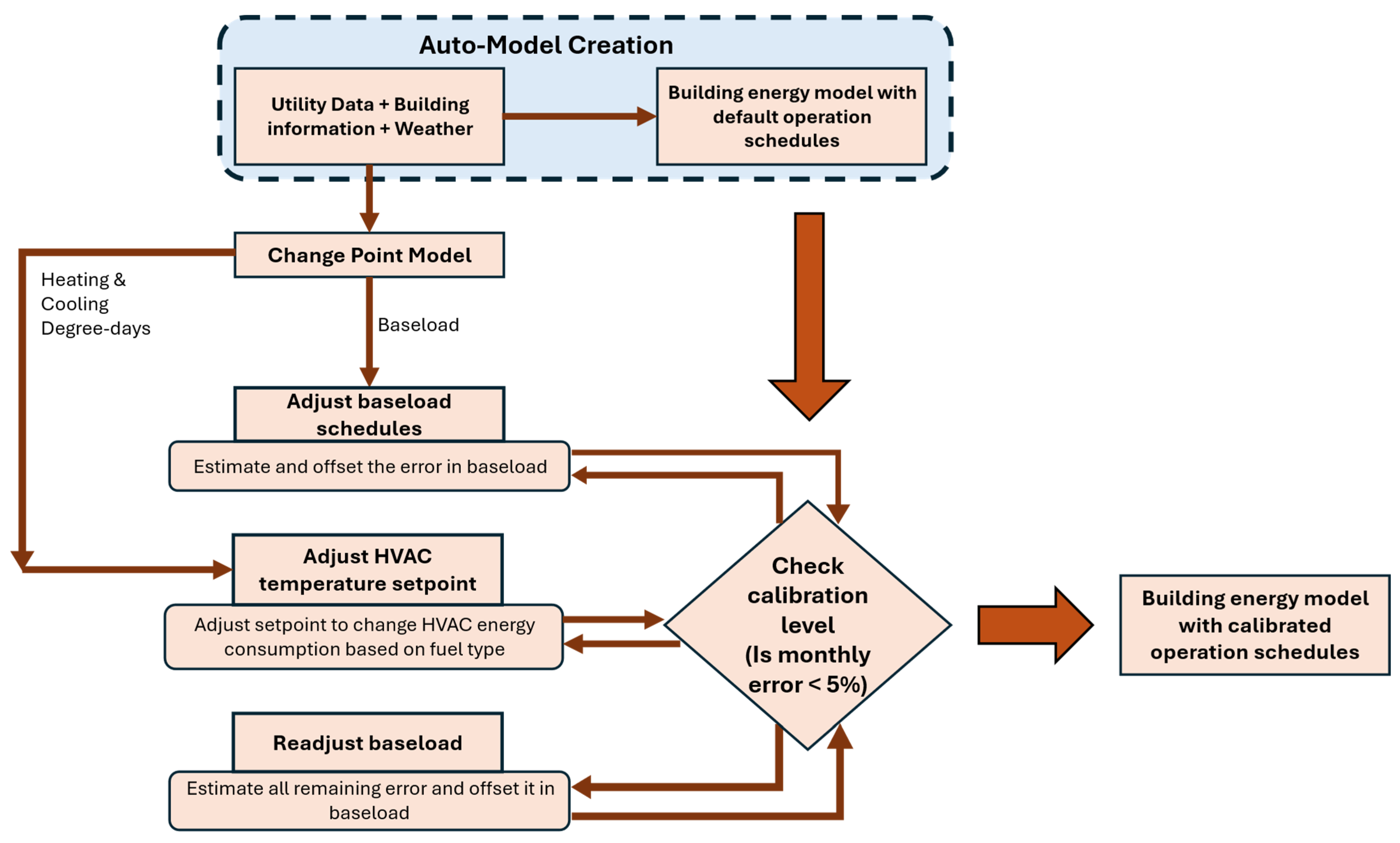
The initial predictions from the developed preliminary energy model for the existing building are based on default operation schedules and thus may not match the utility data entered by the user into the SABER input screens. The actual operating schedules for any building are often challenging to determine since a significant amount of monitored data is required to pinpoint actual occupancy levels, lighting on/off status, and indoor temperature settings. SABER overcomes this difficulty by adjusting the default operation schedules sequentially using an automated calibration algorithm based on information inferred from the utility data. As summarized in Figure 4, the building energy model calibration is accomplished by SABER using three steps.

Figure 4. Description of automatic schedule calibration algorithm used in SABER.

First, the baseload energy consumption levels are adjusted to the values estimated from the utility data analysis. Second, the monthly HVAC energy demands are adjusted by changing the temperature setpoints appropriately. Finally, the remaining prediction discrepancies between the modeled and actual monthly energy usages are reduced by readjusting the baseload levels. For each month, the relative differences between the model predictions and utility data for electricity (${\delta }_E^i$) and natural gas (${\delta }_G^i$) are estimated as shown in Equations (1) and (2):

$${\delta }_E^i={\displaystyle \frac{{\widehat{E}}^i-E^i}{{\widehat{E}}^i}}$$

(1)

$${\delta }_G^i={\displaystyle \frac{{\widehat{G}}^i-G^i}{{\widehat{G}}^i}}$$

(2)

where ${\widehat{E}}^i$ and ${\widehat{G}}^i$ are the electricity and natural gas consumption predicted by the simulation model, and $E^i$ and $G^i$ are the values obtained from the utility data for month i.

In SABER, the building energy model is said to be calibrated when its prediction errors, ${\delta }_E^i$ and ${\delta }_G^i$, do not exceed a predefined threshold of 5%. These calibration thresholds are slightly more stringent that the requirements set by the ASHRAE Guideline 14 [37]. The details of the calibration method implementation are provided in the following sections.

4.1. Adjustment of Baseload Energy Consumption

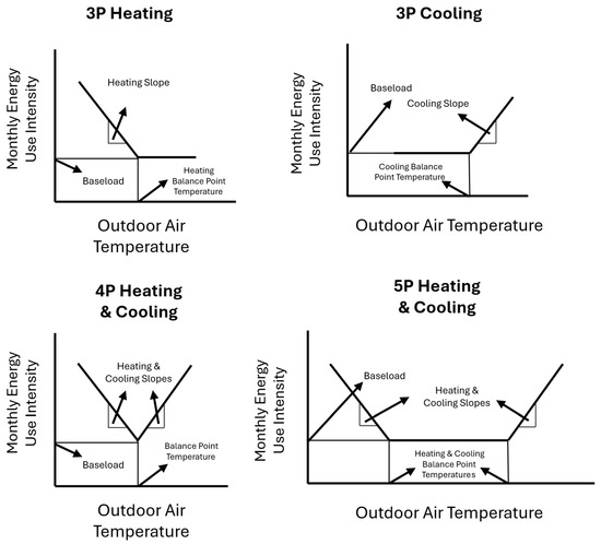
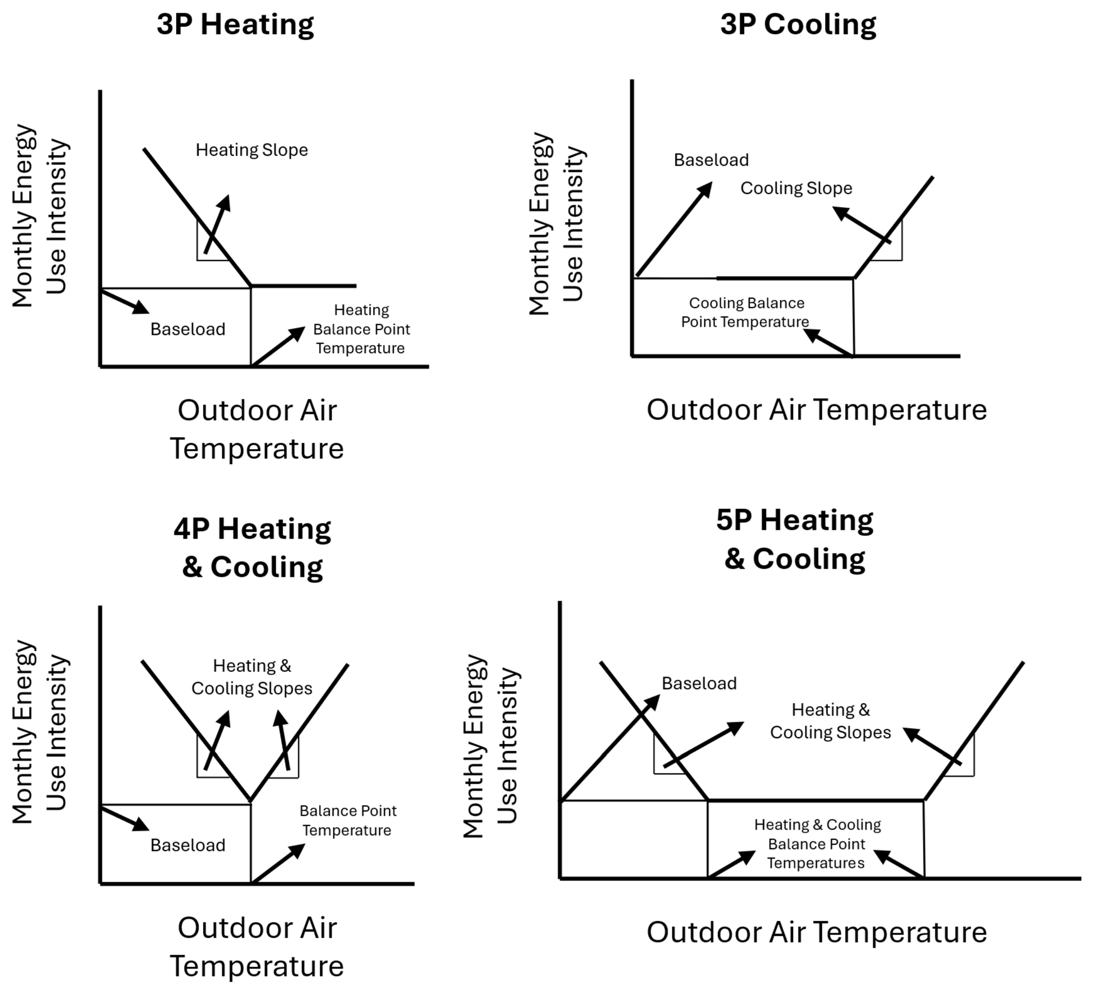
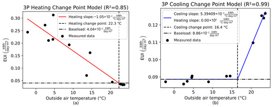
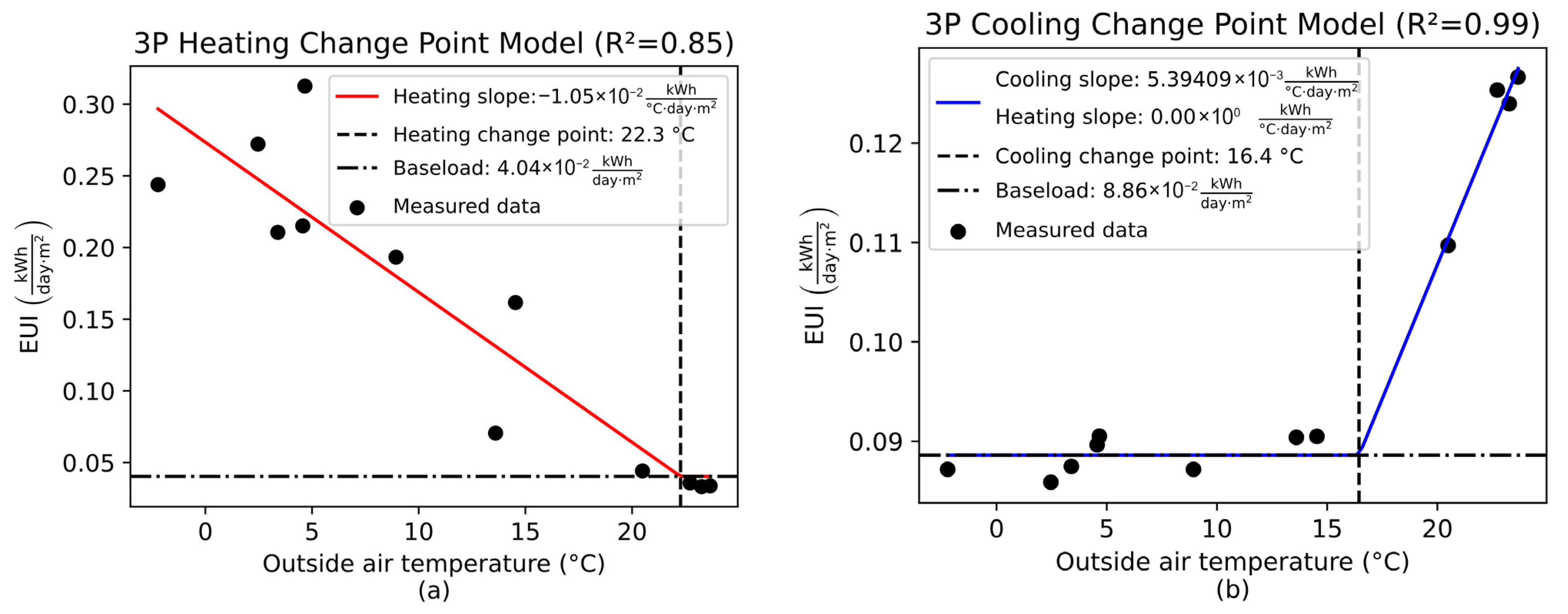
The automated calibration approach of SABER utilizes the results obtained from the energy signature analysis of a building using change point models [38]. Change point models fit a piecewise linear regression model between the building’s energy consumption and various outdoor weather variables, including the outdoor air temperature and heating or cooling degree-days. Figure 5 shows the temperature-based change point for a residential building case study located in US climate zone 5B [39]. A change point model for any building is defined at most by five parameters, namely, the heating and cooling balance point temperatures, heating and cooling slopes, and the baseload energy consumption. The balance point temperatures represent the outdoor air temperature at which no additional heating or cooling is required to maintain indoor thermal comfort. The heating and cooling slopes represent the additional heating or cooling required due to a unit change in the outdoor air temperature. Finally, the baseload energy consumption represents the baseline energy consumption of the building throughout the year, irrespective of the outdoor weather conditions. In the case of electricity, the baseload typically corresponds to lighting and electric equipment energy end-uses, and in the case of natural gas to domestic hot water and cooking energy needs.

Figure 5. Temperature-based change point models with 3, 4, and 5 parameters.

Change point models have previously been used to calibrate energy models [40] and to evaluate the impact of energy conservation measures [41]. For instance, Kim and Haberl [40] used the relative change in the change point model parameters as the yardstick to calibrate the input parameters of an energy model of a residential building using the DOE2.1E simulation engine. In SABER, the change point model is used to estimate the energy use baseloads for an evaluated building. Indeed, the baseload energy consumption does not vary significantly throughout the year, irrespective of outdoor air temperatures, as it includes only non-HVAC energy end-uses. For instance, Equation (3) estimates the monthly electricity baseloads when only lighting and electrical equipment are considered as the corresponding non-HVAC systems.

$$E_{Base}^i=E_{Ltg}^i+E_{ElecEqp}^i$$

(3)

where $E_{Ltg}^i$ and $E_{ElecEqp}^i$ are the lighting and electric energy consumption in month $i,$ respectively. In most detailed whole-building energy simulation analysis tools, including EnergyPlus, each of these monthly energy consumptions are computed as a summation of a fraction of usage and the rated power consumption, as depicted by Equations (4) and (5).

$$E_{Ltg}^i=N_{wkdy}\sum _{h=1}^{24}{f}_{Ltg,wkdy}^{ih}{P}_{Ltg}+N_{wknd}\sum _{h=1}^{24}{f}_{Ltg,wknd}^{ih}{P}_{Ltg}$$

(4)

$$E_{ElecEqp}^i=N_{wkdy}\sum _{h=1}^{24}{f}_{ElecEqp,wkdy}^{ih}{P}_{ElecEqp}+N_{wknd}\sum _{h=1}^{24}{f}_{ElecEqp,wknd}^{ih}{P}_{ElecEqp}$$

(5)

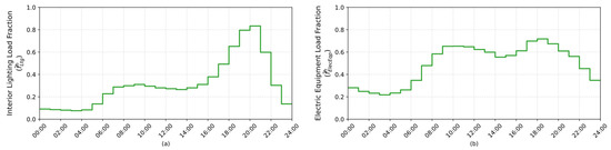
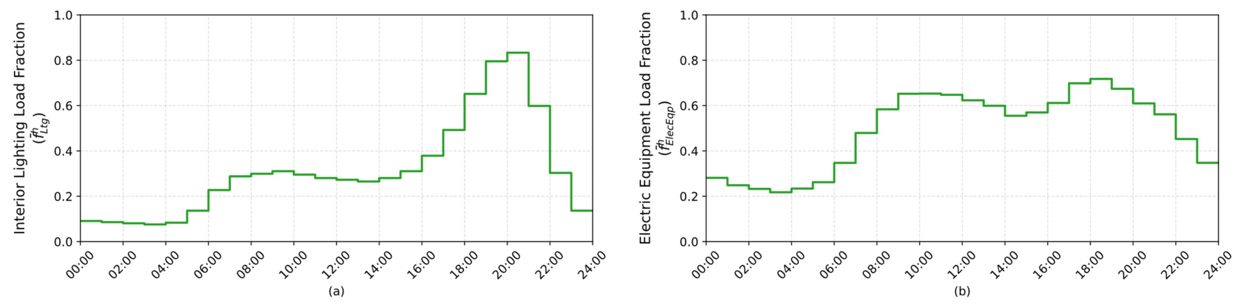
where $f_{Ltg,wkdy}^{ih}$, $f_{Ltg,wknd}^{ih}$, $f_{ElecEqp,wkdy}^{ih}$, and $f_{ElecEqp,wknd}^{ih}$ are the fractions of rated power consumption for lighting and electric equipment during the $h^{th}$ hour of the $i^{th}$ month for a weekday and weekend, respectively, and $P_{Ltg}$ and $P_{ElecEqp}$ are the rated hourly lighting and electric equipment power demands. In SABER, the energy end-uses of different electric equipment, including clothes washer, dryer, dishwasher, cooking range, refrigerator, and miscellaneous plug loads, are computed separately using Equation (5). Figure 6 shows examples of the mean daily lighting and electric equipment schedules for a weekday applied by default when generating energy models for residential buildings before any calibration is initiated.

Figure 6. Mean load fraction values for (a) interior lighting and (b) electric equipment used as initial default weekday schedules for single-family residential buildings in SABER.

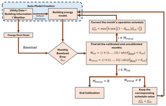
To adjust the baseload energy consumption, SABER adjusts the value of load fraction of each electric and gas piece of equipment that contributes to the baseload energy consumption. As shown in Figure 7, SABER uses the results of the change point model to correct the baseload for both electricity and natural gas separately.

Figure 7. Algorithm used to adjust baseload energy consumption in SABER.

The errors between the monthly energy use baseloads calculated from the change point model illustrated in Figure 5 and those predicted by the generated building energy model can be used to adjust the usage fraction values for each of the schedules. Equations (6) and (7) are used to calculate the errors in the baseload energy consumption for electricity and natural gas:

$${\delta }_{E,Base}^i={\displaystyle \frac{{\widehat{E}}_{Base}^i-E_{Base}}{{\widehat{E}}_{Base}^i}}$$

(6)

$${\delta }_{G,Base}^i={\displaystyle \frac{{\widehat{G}}_{Base}^i-G_{Base}}{{\widehat{G}}_{Base}^i}}$$

(7)

where $E_{Base}$ and $G_{Base}$ are the mean monthly baseload values obtained from the change point model, ${\delta }_{E,Base}^i$ and ${\delta }_{G,Base}^i$ are the relative errors in the baseload, and ${\widehat{E}}_{Base}^i$ and ${\widehat{G}}_{Base}^i$ are the values of monthly baseload as predicted by the simulation model. After estimating the electricity and natural gas baseload errors for each month, all the months where the absolute error is less than a given threshold $\left({\delta }_{Cal}\right)$ are categorized as calibrated months $\left(M_{Cal}\right),$ and the rest are categorized as uncalibrated months $\left(M_{UnCal}\right)$, as shown in Figure 7. For the uncalibrated months $\left(M_{UnCal}\right),$ the load fraction values for each of the schedules are adjusted based on Equation (8):

$${\mathit{f}}_{Sch}^{*i}=max\left(0,min\left(\left(1-{\delta }_{Base}^i\right){\mathit{f}}_{Sch}^i,1\right)\right)$$

(8)

$${\mathit{f}}_{Sch}^i=\left[\begin{array}{cccc}{f}_{Sch,wkdy}^{i1}& f_{Sch,wkdy}^{i2}& \cdots & f_{Sch,wkdy}^{i24}\\ f_{Sch,wknd}^{i1}& f_{Sch,wknd}^{i2}& \cdots & f_{Sch,wknd}^{i24}\end{array}\right]$$

(9)

where $f_{Sch}^i$ is the matrix containing the load fraction value of each corresponding schedule for the $i^{th}$ month in the current iteration for each hour of a weekday and weekend, as show in Equation (9); and $f_{Sch}^{*i}$ is the corrected value. Depending on the end-use of the schedule, the baseload error can refer to either electricity or natural gas. So, for instance, for the case of lighting and electric equipment schedules, ${\delta }_{Base}^i$ refers to the error in the electricity baseload consumption calculated using Equation (6). For the case of domestic hot water and gas-based cooking schedules, ${\delta }_{Base}^i$ refers to the error in the natural gas baseload consumption.

Therefore, if the baseload value of a particular energy source calculated from the change point model is 50% lower than the value from the model predictions, then the corresponding load fraction values of each schedule are multiplied by 0.5. Equation (8) ensures that adjustments of the schedules are restricted to between a minimum value of 0 and a maximum value of 1. The same procedure is used to adjust the domestic hot water and cooking energy consumption to calibrate the monthly baseloads for natural gas and other energy sources.

4.2. Adjustment of Heating and Cooling Temperature Setpoints

After adjusting the monthly electricity and natural gas baseloads, the remaining model prediction errors are associated with estimating the HVAC energy consumption. The HVAC energy consumption of a building is primarily controlled by the heating and cooling temperature setpoints. To provide more flexibility to the calibration algorithm, SABER adjusts the temperature setpoints on a monthly basis rather than yearly or seasonally. Before adjusting the temperature setpoints, each month is first assigned to one of three types, heating dominated, cooling dominated, and neutral, as shown in Equations (10) and (11). Both the cooling ($CD{D}_i$) and heating degree days ($HD{D}_i$) for each month, calculated based on the balance point temperatures obtained from the change point model, are used to determine the month’s type.

$$M^H=\left\{i\in \left\{1,\dots 12\right\}|{\displaystyle \frac{HD{D}_i}{HD{D}_i+CD{D}_i}}>{\delta }_{DD}\right\}$$

(10)

$$M^C=\left\{i\in \left\{1,\dots 12\right\}|{\displaystyle \frac{HD{D}_i}{HD{D}_i+CD{D}_i}}<{\delta }_{DD}\right\}$$

(11)

where the heating and cooling degree days are calculated as follows,

$$HD{D}_i=\sum _{d=1}^{N_i}max\left(T_b^H-T_o^d,0\right)$$

(12)

$$CD{D}_i=\sum _{d=1}^{N_i}max\left(T_o^d-T_b^C,0\right)$$

(13)

where $T_b^H$ and $T_b^C$ are the heating and cooling balance point temperatures obtained from the change point model, $T_o^d$ is the daily mean outdoor air temperature, and $N_i$ is the total number of days in month $i$. A threshold, ${\delta }_{DD},$ is chosen to categorize whether a month is heating or cooling dominated. The value of this threshold is always between 0 and 1; a default value of 0.25 is used in SABER.

Based on whether a month is heating or cooling dominated, only the corresponding temperature setpoint is adjusted. For neutral months, both the heating and cooling temperature setpoints are adjusted. The adjustment of the setpoint value in each month is dependent on the error in the natural gas (${\delta }_G^i$) and electricity consumption (${\delta }_E^i$) predictions, as calculated using Equation (1) and Equation (2), respectively.

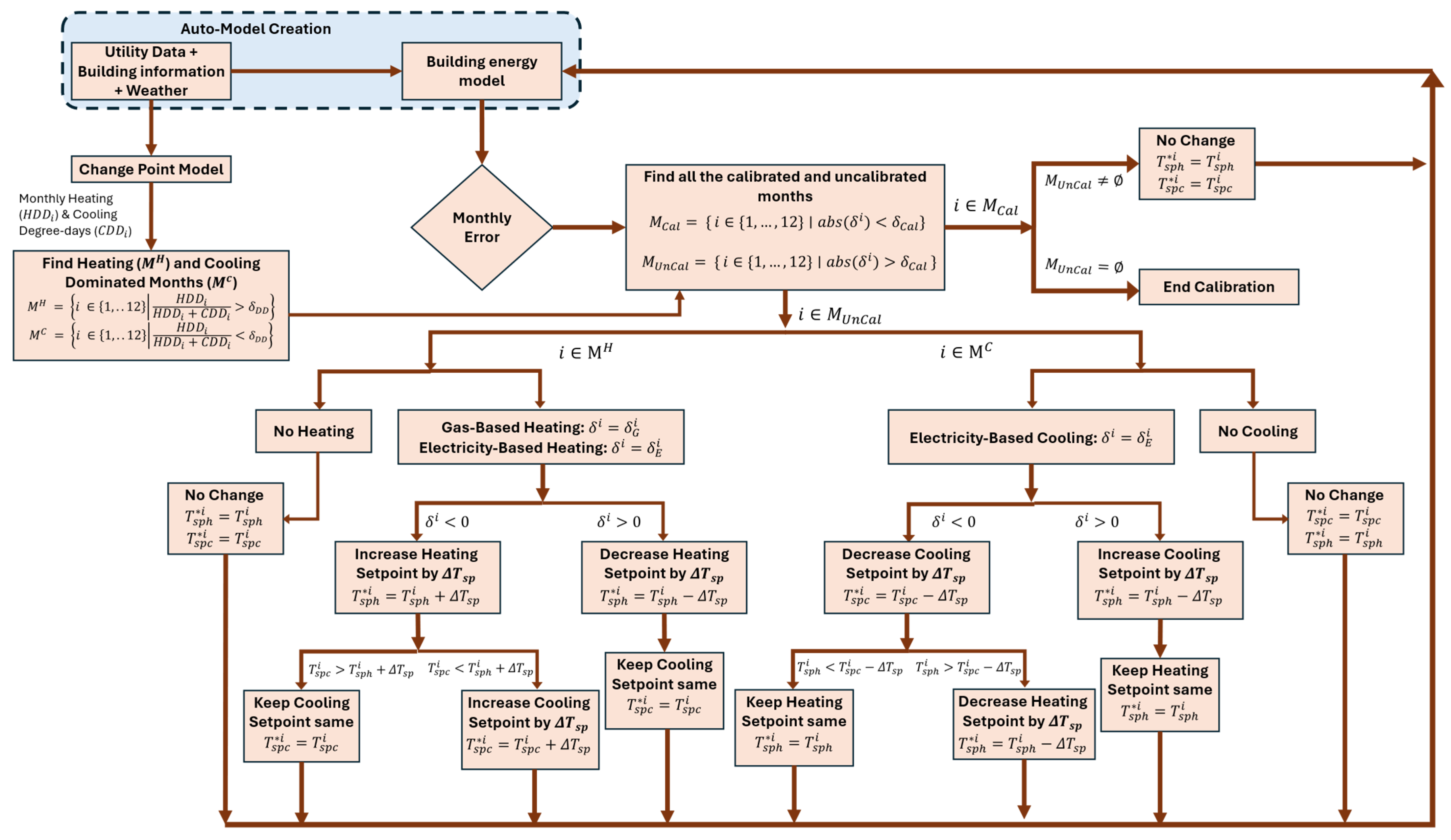
The monthly energy consumption predicted by the building model depends on the heating and cooling temperature setpoints, denoted by $T_{sph}^i$ and $T_{spc}^i$, respectively. The calibration process of the energy model, which adjusts the heating and cooling temperature setpoints, is conducted using multiple iterations as illustrated in Figure 8. At the beginning of each iteration, the error values ${\delta }_E^i$ and ${\delta }_G^i$ are calculated using Equation (1) and Equation (2), respectively. Depending on the magnitude of the errors, the months are categorized into calibrated and uncalibrated months based on the threshold, ${\delta }_{Cal}$. Therefore, each month has two labels, one to indicate if it is calibrated and one to indicate if it is heating or cooling dominated. For each of the uncalibrated months, based on the dominating HVAC energy end-use, the corresponding schedule is adjusted. If the error in that month is positive that means the simulated energy consumption is more than the utility data value and so must be reduced. To do so, the heating temperature setpoint is decreased by a given $\Delta T_{sp}$ in a heating-dominated month and the cooling temperature setpoint is increased by $\Delta T_{sp}$ in a cooling-dominated month and vice versa. In the case of gas-based heating temperature setpoint adjustment, the value of ${\delta }_G^i$ triggers a change in the setpoint, whereas for an electricity-based heating system (such as a heat pump), the value of ${\delta }_E^i$ triggers a change in the heating temperature setpoint. Finally, a change in the heating or cooling temperature setpoints is carried out only under the condition that the cooling setpoint is always greater than the heating setpoint. Therefore, in a heating-dominated month, if increasing the heating temperature setpoint would cause its value to be greater than the cooling temperature setpoint, then both the heating and cooling setpoints are increased by $\Delta T_{sp},$ thereby maintaining the dual setpoint band. Conversely, in a cooling-dominated month, if decreasing the cooling temperature setpoint would cause its value to be less than the heating temperature setpoint, then both setpoints are simultaneously decreased.

Figure 8. Algorithm flowchart used to adjust HVAC energy consumption in SABER.

As stated previously, the adjustment of temperature setpoints is an iterative process, with the errors being recalculated and updated after each iteration. When the model prediction error for the building energy use for a given month is less than ${\delta }_{Cal}$, then that month is dropped from the calibration process but adjustments of temperature setpoints continue for the remaining months. In SABER, adjustments of temperature setpoints for all months are set to remain within reasonable ranges, defined to be between 10 °C and 25 °C for heating and 15 °C and 35 °C for cooling. These bounds are set as default limits to ensure that indoor thermal comfort levels can be achieved for most building types. However, these default upper and lower limits for temperature setpoints can be reset by the user. The normalized total squared error is used as a metric to keep track of the accuracy level of the calibration process, as shown in Equation (14). Temperature setpoint adjustments are carried out if the calibration accuracy level continues to improve after each iteration or until the building energy usage for all months is calibrated with the set tolerance (i.e., ${\delta }_{Cal}= 5\%$).

$$S=\sqrt{\sum _{i=1}^{12}\left({\left({\delta }_E^i\right)}^2+{\left({\delta }_G^i\right)}^2\right)}$$

(14)

4.3. Baseload Readjustment

Even after the correction of heating and cooling temperature setpoints, the model prediction errors could still remain above the set tolerance (${\delta }_{Cal}$) for a few months of the year. The source of the remaining errors could be due to several reasons, from uncertainty in the building energy simulation parameter estimates to the temperature setpoint adjustments conducted at $\Delta T_{sp}$ intervals. To finalize the calibration of the energy model, any remaining significant errors are reduced by readjusting the baseloads. The same calibration process outlined in Figure 7 is used for readjusting the baseloads with the remaining errors ${\delta }_E^i$ and ${\delta }_G^i$, as calculated by Equations (1) and (2), set as the references in place of ${\delta }_{Base}^i$.

4.4. Verification of Automatic Calibration Approach

To verify the performance of the automatic calibration algorithm, the calibration of well-established prototypical residential building energy model is considered [39]. The main features of a prototypical building specific to climate region 5B are given in Table 3. Figure 9 shows the results of the energy simulation using EnergyPlus for both electricity and natural gas throughout the year. These simulation results are used as the reference utility data to verify the calibration algorithms implemented in SABER outlined in Section 4.1, Section 4.2 and Section 4.3.

Table 3. Main characteristics of prototypical residential building energy model in climate region 5B used for verification analysis of SABER’s calibration algorithm.

Property	Value
Total Floor Area	$331 \mathrm{s}\mathrm{q}\mathrm{m}\left(3566 \mathrm{s}\mathrm{f}\mathrm{t}\right)$
Exterior Wall	Synthetic stucco/sheathing/${\displaystyle \frac{7}{16}} \mathrm{i}\mathrm{n}.$ OSB/R13 wall insulation/$0.5 \mathrm{i}\mathrm{n}.$ drywall
Foundation	Concrete slab-on-grade floor
Roof	Asphalt shingles with R40 ceiling insulation
Window	Standard glass with U factor of $1.7 \mathrm{W}/{\mathrm{m}}^2\mathrm{K}$ and SHGC of $0.33$ with interior blinds
Window-To-Wall Ratio	14.12% (2 windows on each wall)
Number Of Occupants	$3$
Electric Equipment	Dishwasher ($65.7 \mathrm{W}$), refrigerator ($91.05 \mathrm{W}$), clothes washer ($28.47 \mathrm{W}$), clothes dryer ($213.06 \mathrm{W}$), misc. electric equipment ($507.14 \mathrm{W}$), misc. plug loads ($2.28 \mathrm{W}/{\mathrm{m}}^2$)
Gas Equipment	Cooking range ($540 \mathrm{W}$)
Lighting Power Density	Hardwired ($1.05 \mathrm{W}/{\mathrm{m}}^2$), plug-in ($0.47 \mathrm{W}/{\mathrm{m}}^2$)
Temperature Setpoint	Heating setpoint—22.222 °C (72 °F) Cooling setpoint—23.888 °C (75 °F)
Heating Equipment	Gas furnace (80% AFUE)
Cooling Equipment	Air conditioner (13 SEER)
Hot Water Equipment	Gas boiler (92% AFUE)

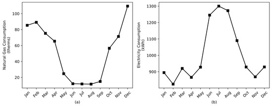
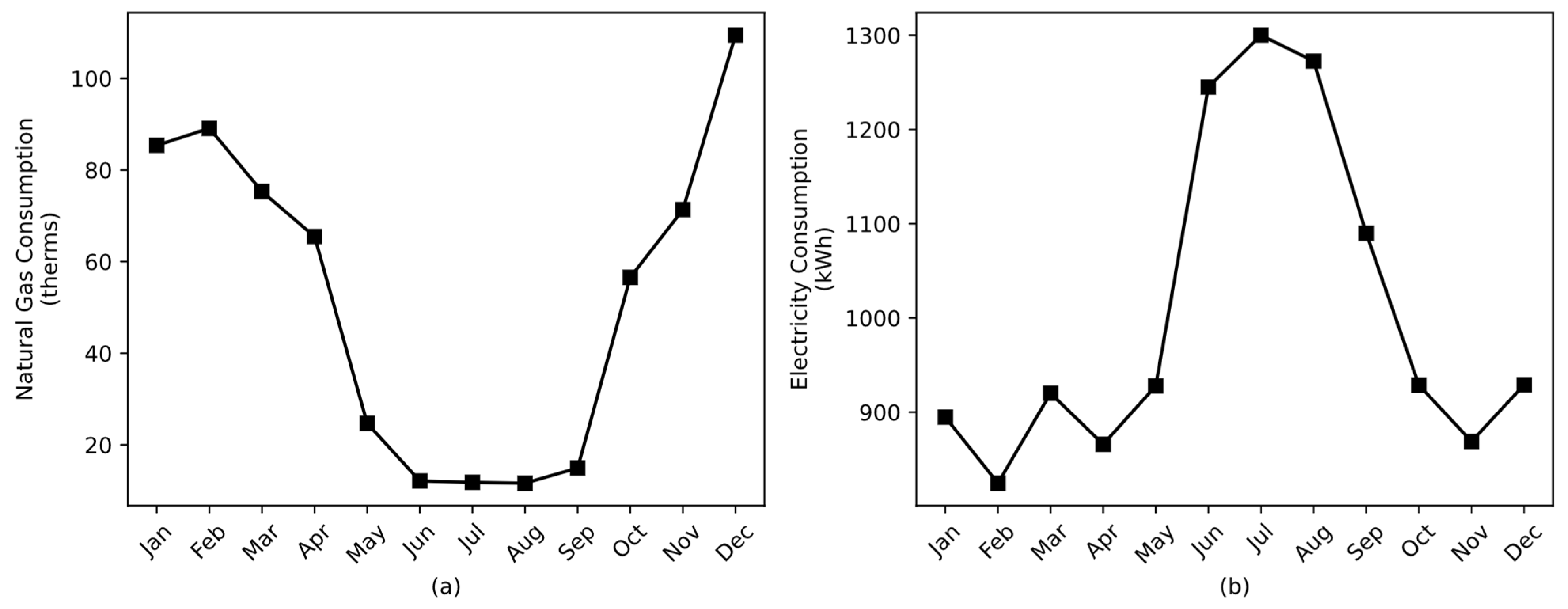
Figure 9. Monthly (a) natural gas and (b) electricity use of prototypical residential building model with constant baseloads.

To verify the calibration algorithm, the default schedules defined in SABER are used to develop an energy model for a prototypical residential building in addition to the input data listed in Table 3. Using the utility data outlined in Figure 9, SABER is used to conduct an energy signature analysis of this residential building using the temperature and degree day-based change point models. The temperature-based change point models for both electricity and natural gas data are illustrated in Figure 10.

Figure 10. Temperature-based change point models for (a) natural gas and (b) electricity consumption for prototypical residential building case study in climate zone 5B.

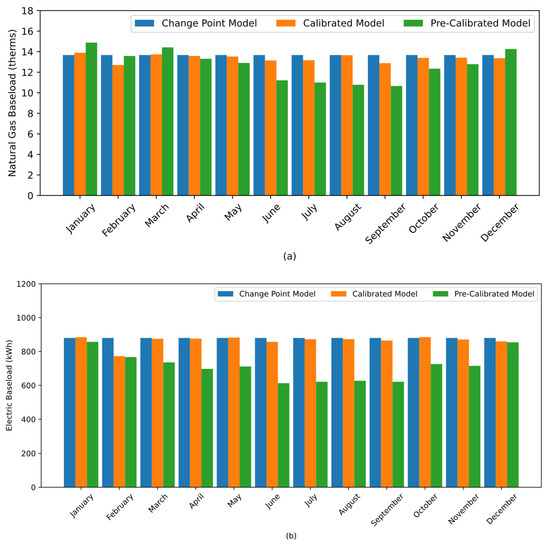
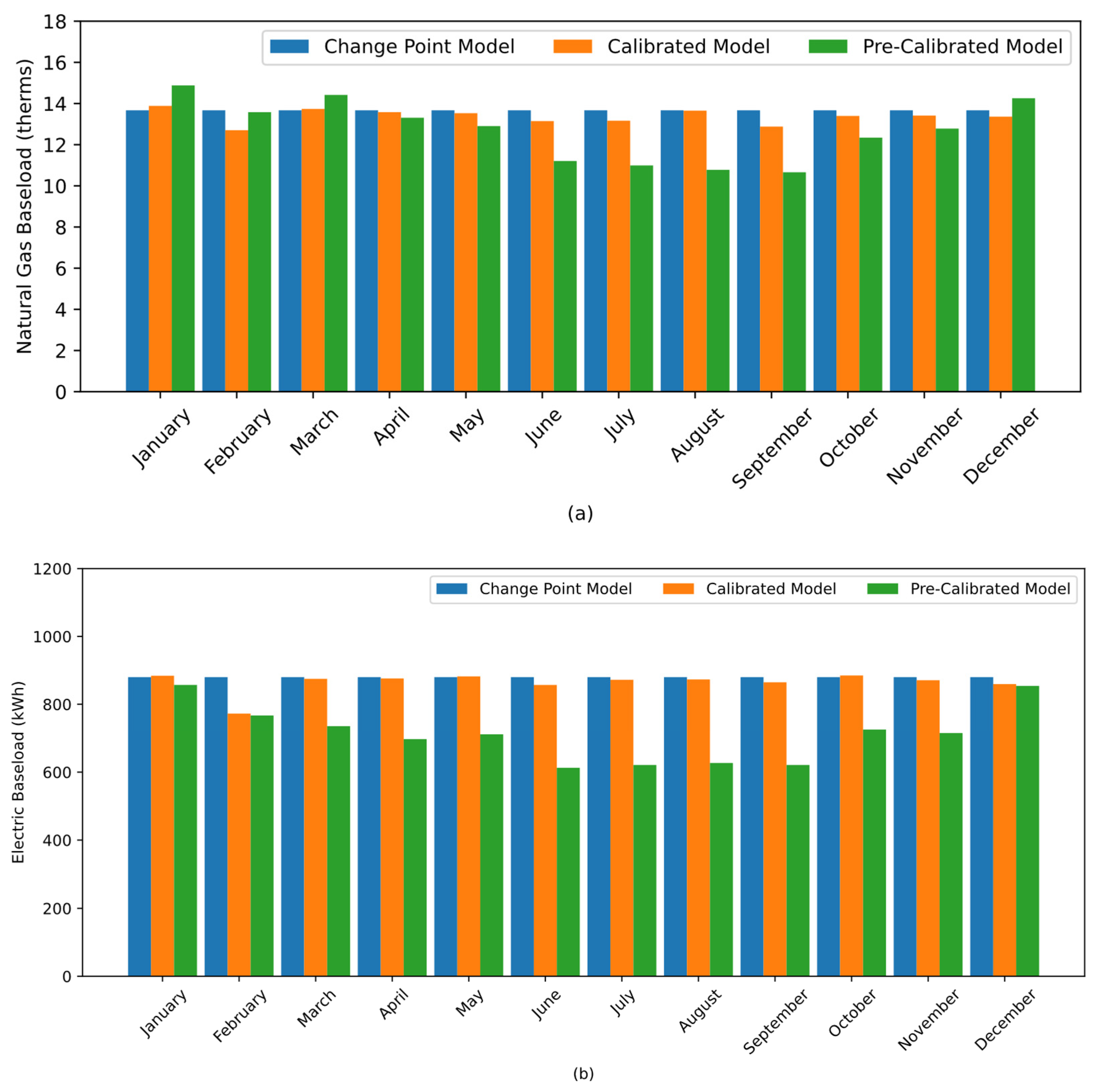
As indicated in Figure 10, the monthly baseloads for this prototypical residential building are estimated to be 879.97 kWh for electricity and 13.67 therms for natural gas. SABER adjusts the schedules for lighting, electric equipment, domestic hot water, and cooking using the calibration approach method described in Section 4.1 to match the baseload values obtained from the change point model. Figure 11 shows the monthly variation in the natural gas and electricity baseloads before and after the calibration process is completed, along with the reference values estimated from the utility data using change point modeling. For most of the months, the pre-calibrated schedules almost consistently underpredict the baseloads estimated from the utility data.

Figure 11. Monthly variation in baseloads for (a) natural gas and (b) electricity consumption for pre- and post-calibrated energy models, along with reference baseload values obtained from change point model analysis of utility data. Proposed calibration algorithm approaches baseload values estimated from change point models of both energy sources.

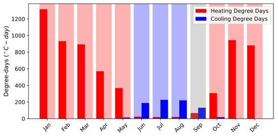
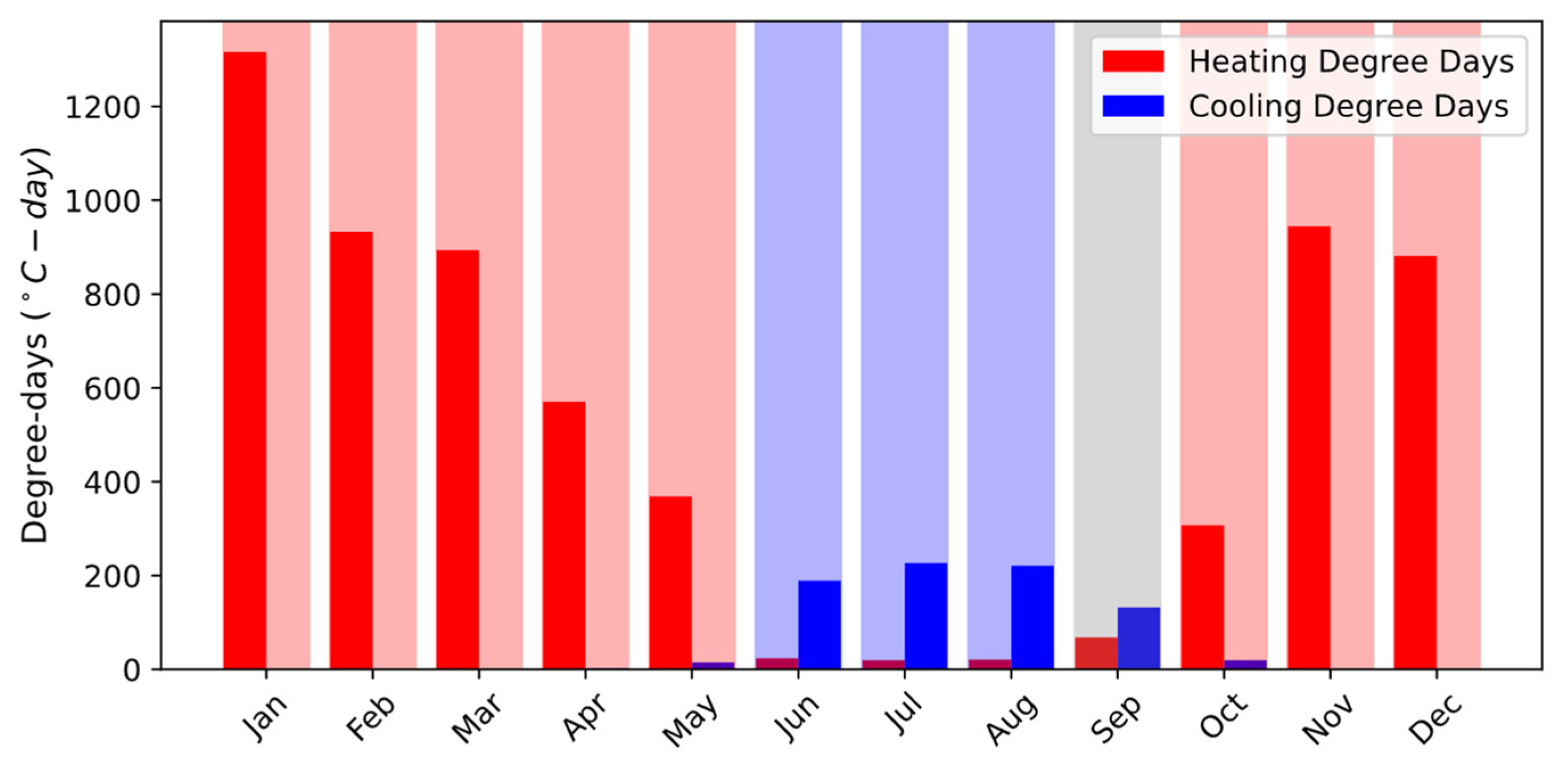
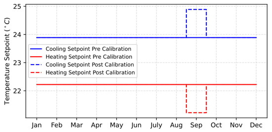
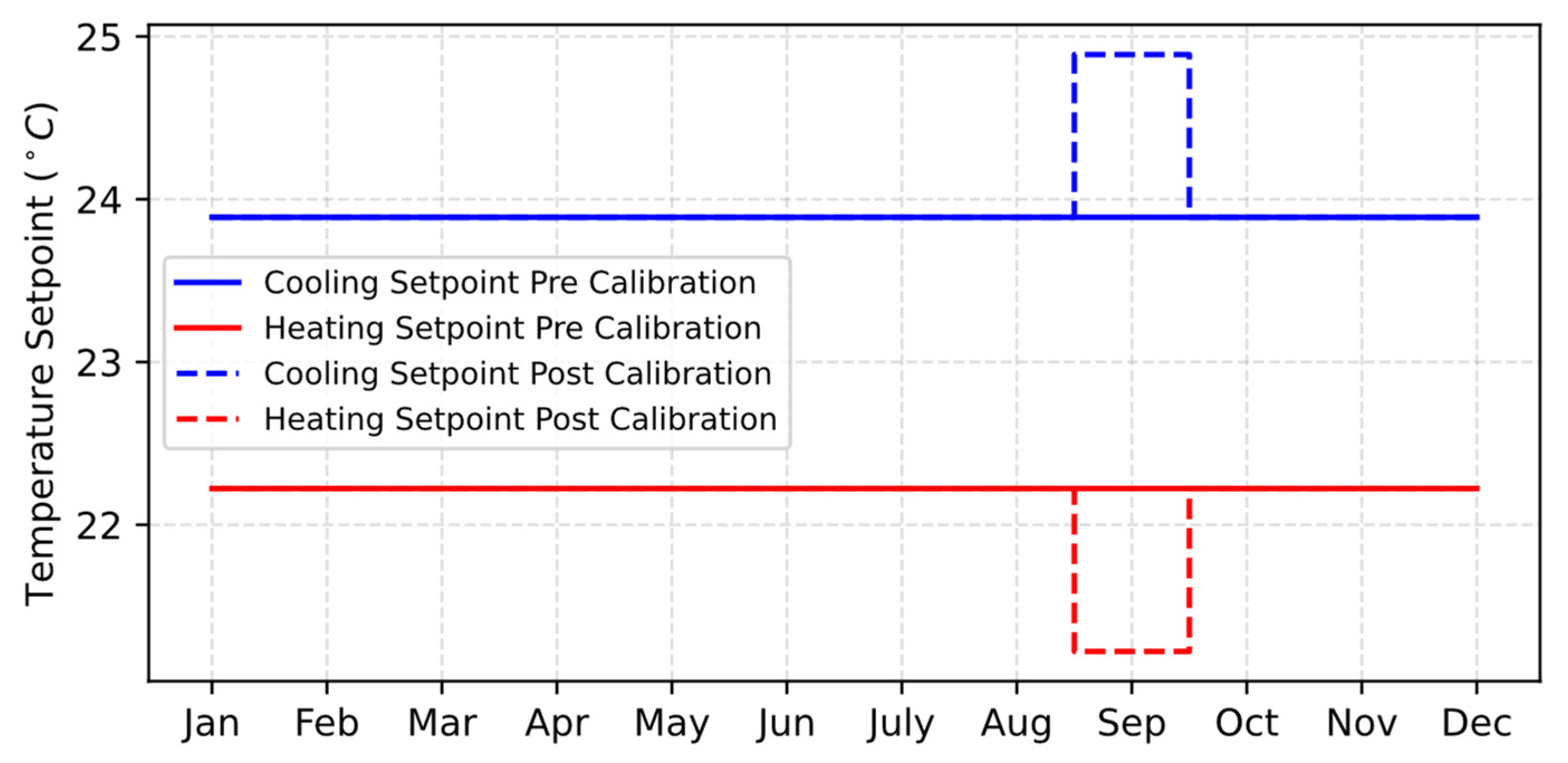
To adjust the HVAC energy end-use, all the months of the year are first segregated into heating- and cooling-dominated categories based on the number of heating and cooling degree days calculated using the best-fit change point model, as shown in Figure 12. Using the classification and the algorithm described in Section 4.2, the final temperature setpoint schedules are adjusted, as shown in Figure 13.

Figure 12. Number of heating and cooling degree days calculated using the change point model, along with their classification into neutral (in grey) and heating- (in red) and cooling-dominated months (in blue).

Figure 13. HVAC temperature setpoint schedule for each month before and after calibration, showing minimal deviations.

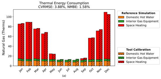
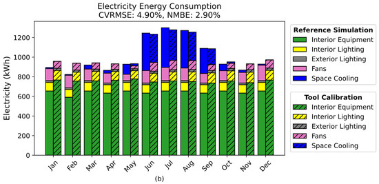
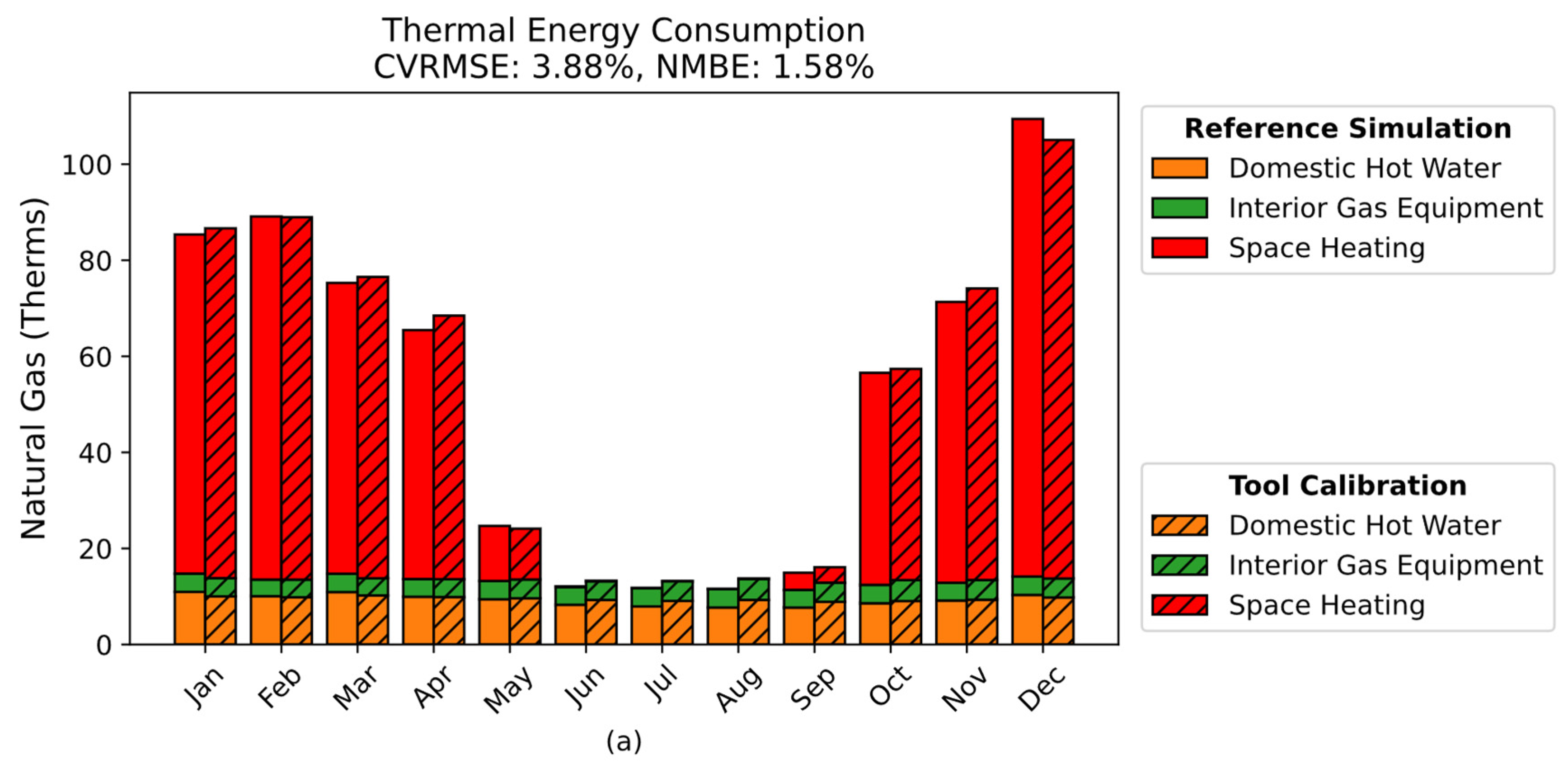
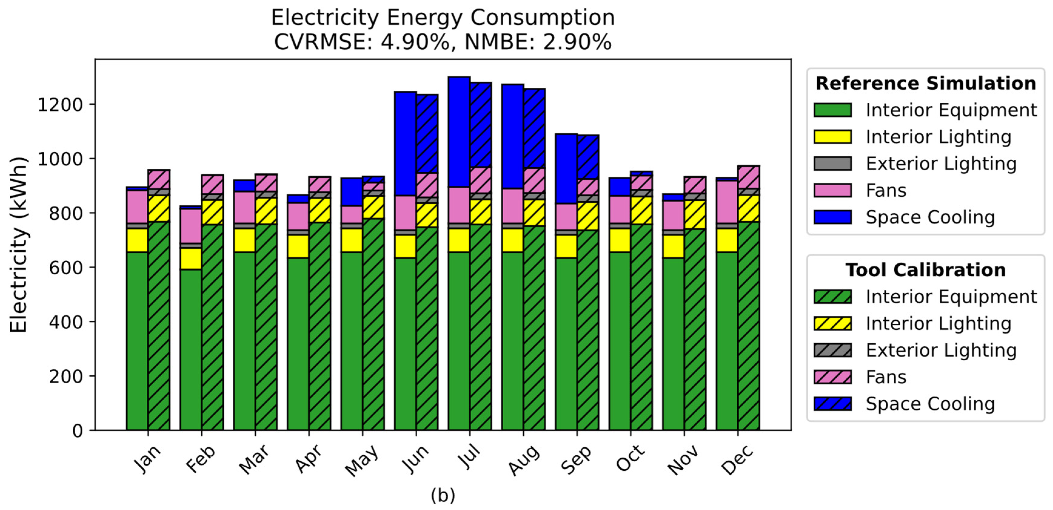
Finally, the remaining errors are lowered using the baseload readjustment approach described in Section 4.3, and the calibration process of energy mode defined in SABER is completed. Figure 14 compares the end-use energy distributions of the final building energy models determined by SABER using the proposed automated calibration algorithm. The striped bars represent the results obtained from the tool calibration while the solid bars represent the end-use distributions obtained from the direct simulation of the prototypical reference building energy model. For both electricity and natural gas, the Coefficient of Variation of Root Mean Squared Error (CVRMSE) and Normalized Mean Bias Error (NMBE) both lie within the requirements set by the ASHRAE Guideline 14 [37] for monthly calibration. Furthermore, Table 4 compares the total number of equivalent full-load hours from the reference and calibrated energy models. The calibrated model overestimates the lighting and equipment electricity use levels but underestimates the domestic hot water natural gas use. However, these deviations are compensated for by adjustments in the cooling and heating energy end-uses.

Figure 14. Comparison of results of calibrated simulated model obtained from SABER against prototypical residential building simulation data, with constant baseload used as calibration reference for (a) natural gas consumption and (b) electricity consumption.

Table 4. Comparison of total number of equivalent full-load hours for various schedules from reference and SABER-calibrated models.

Month	Interior Lighting		Electric Equipment		Domestic Hot Water
	Reference Simulation	Tool Calibration	Reference Simulation	Tool Calibration	Reference Simulation	Tool Calibration
January	9.12	8.66 (−5%)	98.03	93.14 (−5%)	8.55	8.09 (−5%)
February	8.51	8.51 (0%)	98.35	98.35 (0%)	8.55	8.55 (0%)
March	7.82	8.69 (+11%)	84.77	91.39 (+8%)	8.55	6.47 (−24%)
April	7.13	8.02 (+12%)	84.5	89.49 (+6%)	8.55	3.75 (−56%)
May	6.44	7.12 (+11%)	84.77	90.76 (+7%)	8.55	6.9 (−19%)
June	6.13	8.87 (+45%)	75.29	103.36 (+37%)	8.55	8.24 (−4%)
July	6.28	8.97 (+43%)	75.13	101.99 (+36%)	8.55	8.28 (−3%)
August	6.74	9.5 (+41%)	75.13	101.23 (+35%)	8.55	8.29 (−3%)
September	7.51	10.44 (+39%)	75.29	103.1 (+37%)	8.55	9.65 (+13%)
October	8.2	8.98 (+10%)	85.32	91.61 (+7%)	8.55	6.7 (−22%)
November	8.89	9.57 (+8%)	85.12	89.97 (+6%)	8.55	4.89 (−43%)
December	9.2	9.2 (0%)	98.03	98.03 (0%)	8.55	8.55 (0%)
Annual	91.9	106.5 (+16%)	1019.7	1152.4 (+13%)	102.6	88.36 (−14%)

4.5. Sensitivity of Calibration Metrics Using ${\delta }_{Cal}$ and $\mathit{\Delta }{T}_{sp}$

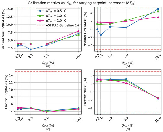
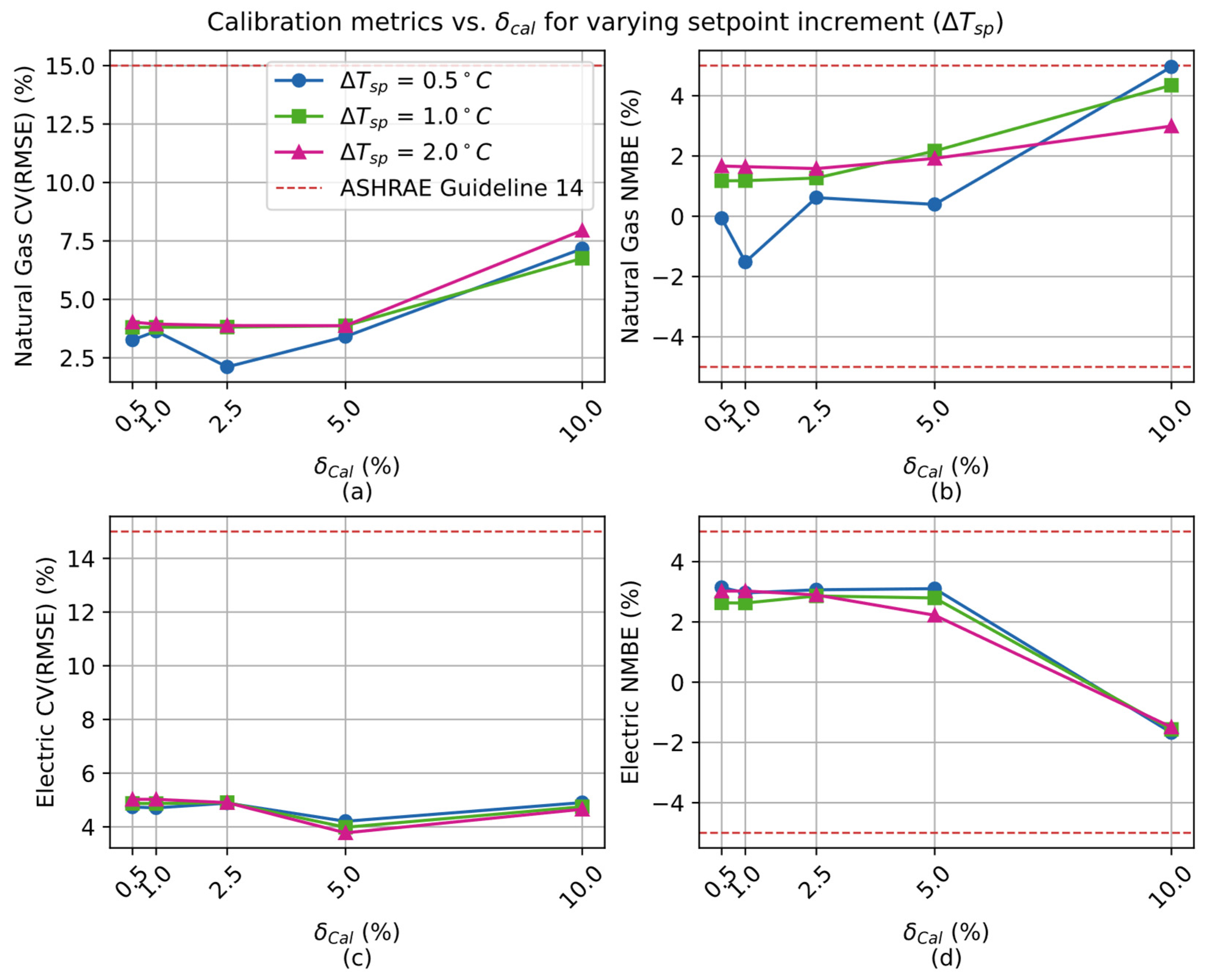
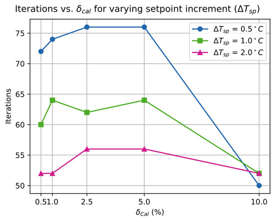
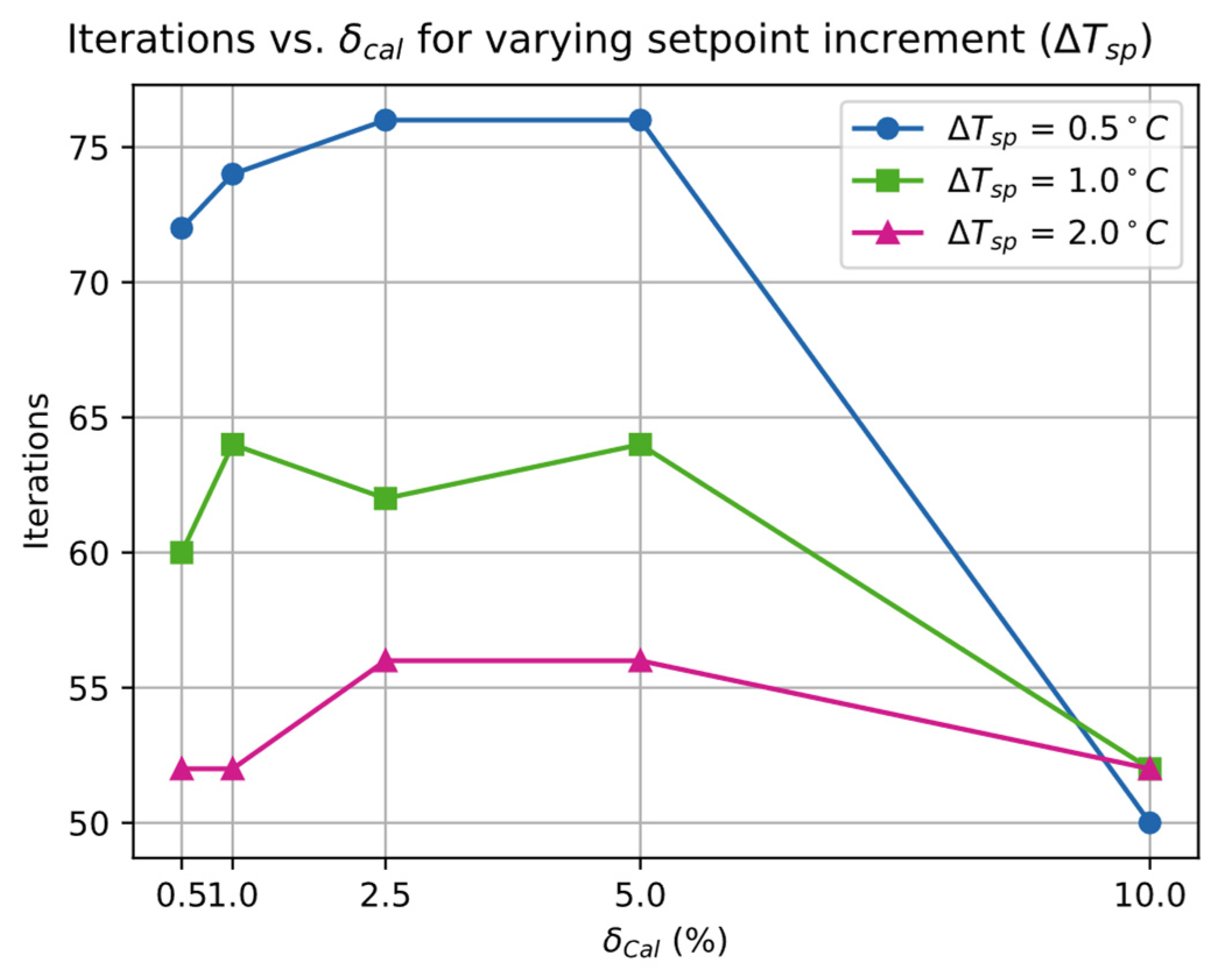
Finally, to verify the impacts of error threshold, ${\delta }_{Cal}$, and the temperature setpoint increment, $\Delta T_{sp}$, on the accuracy of the calibration algorithm, a series of sensitivity analyses is conducted. First, the error threshold value (${\delta }_{Cal}$) is varied from 0.5% to 10% while the temperature setpoint increment, $\Delta T_{sp}$, is changed from 0.5 °C to 2 °C. Figure 15 shows the sensitivity analysis results of model calibration accuracy levels for different error thresholds and temperature setpoint increments. Irrespective of the error threshold chosen, the model is calibrated to within the ASHRAE Guideline 14 requirements for both electricity and natural gas. While the variation in the results for different error thresholds is low, a ${\delta }_{Cal}$ of 10% does have the potential to lead to an uncalibrated model, as shown in Figure 15d. The results shown in Figure 15 indicate that the temperature setpoint increment has a limited effect on the accuracy of calibrated model. Figure 16 shows the number of iterations required for each of the evaluated cases with different combinations of ${\delta }_{Cal}$ and $\Delta T_{sp}$. A higher temperature setpoint increment leads to fewer iterations required for convergence, but a higher error threshold does not necessarily result in fewer iterations. Thus, values of ${\delta }_{Cal}$ of 5% and $\Delta T_{sp}$ of 1 °C are considered the default values for the SABER tool to achieve acceptable model calibration accuracy levels while keeping the number of iterations for convergence to an acceptable degree.

Figure 15. Sensitivity analysis results of (a) CVRMSE for natural gas, (b) NMBE for natural gas, (c) CVRMSE for electricity, and (d) NMBE for electricity to monthly error thresholds and temperature setpoint increments show that all configurations satisfy ASHRAE Guideline 14 requirements.

Figure 16. Number of iterations for convergence for different error thresholds and temperature setpoint increment values. A higher setpoint increment step leads to longer time for convergence.

5. Evaluation of Energy Retrofit Measures

SABER is also capable of evaluating the cost and energy benefits of the deployment of different energy efficiency measures for a building using its calibrated energy model. Specifically, it can model a predefined set of retrofit measures by adjusting the corresponding input parameters within the calibrated energy model. Furthermore, SABER can also evaluate the energy and cost benefits of both individual measures and combinations (i.e., packages) of retrofit measures. Table 5 shows the various energy efficiency measures that are available in the current version of SABER, along with the corresponding description and the change in the EnergyPlus Input Data File (IDF) field required to model each measure.

Table 5. Retrofit measures available in SABER and corresponding IDF field change within EnergyPlus input file.

Measure	Description	IDF Field
Wall Insulation	Improves the exterior wall insulation to the chosen value.	Changes the conductivity of wall insulation material.
Ceiling Insulation	Improves the ceiling insulation to chosen value.	Changes the conductivity of ceiling insulation material.
Window Material	Changes the window material.	Uses the chosen option as the window material to define the window construction.
Infiltration Rate	Reduces the air infiltration.	Changes the effective leakage area by recalculating it based on the chosen value.
Night Setback	Implements a night setback of the heating setpoint.	Changes the value of the daily heating setpoint schedule from 10 pm to 6 am each month by the setback provided.
Daylighting Controls	Implements daylighting controls for lighting system.	Creates a daylighting controls object with the sensor at a location central to the building floor plan.
Percentage LED	Changes the percentage of lighting fixtures using LEDs.	Changes the lighting power density of interior and exterior lighting based on the percentage change in the wattage of fixtures.
Occupancy Sensor	Adds occupancy sensor controls for lighting.	Reduces the lighting schedule by a fixed percentage.
Heating System	Changes system type, efficiency, and capacity of existing heating system.	Replaces the existing HVAC template file with an appropriate one and inputs corresponding efficiency and capacity.
Cooling System	Changes system type, efficiency, and capacity of existing cooling system.	Replaces the existing HVAC template file with an appropriate one and inputs corresponding efficiency and capacity.
Domestic Hot Water System	Changes system type and capacity of existing DHW system.	Replaces the existing DHW template file with an appropriate one and inputs corresponding tank capacity.

The cost and energy metrics are evaluated against each other relative to the calibrated building energy model, giving the user the ability to compare the performance of different retrofit measures. Currently, SABER uses the life cycle cost (LCC) as the metric for the cost-benefit analysis by accounting for both the capital costs required for the implementation of the retrofit measures and the energy costs over the entire lifetime of the retrofit project [42]. The LCC is calculated as indicated by Equation (16) using a user-defined discount rate (d); project lifetime, N; and the uniform series present worth (USPW) factor, as defined by Equation (15):

$$USPW\left(d,N\right)={\displaystyle \frac{1-{\left(1+d\right)}^{-N}}{d}}$$

(15)

$$LCC=IC+USPW\ast EC$$

(16)

where IC is the capital cost needed to implement the individual or packaged measures and EC is the annual energy cost. The default data for the capital costs for various measures are used in the LCC calculations in case the user does not provide this information [31].

Measure Package Optimization

In addition to evaluating the energy and cost benefits of individual and packaged retrofit measures, SABER can also identify the best combination of retrofit measures to minimize a given objective function within a set of constraints. Currently, SABER uses sequential search techniques [36] to optimize the retrofit package, but it is equipped to handle other meta-heuristic techniques, including Genetic Algorithm (GA) [43,44] and Particle Swarm Optimization (PSO) [45], to perform the optimization analysis. The problem of finding the most optimal combination of retrofit measures to minimize a given objective function can be expressed as follows:

$$min \mathit{F}\left(\mathit{X}\right)={\left[f_1\left(\mathit{X}\right),f_2\left(\mathit{X}\right)\dots \right]}^T$$

(17)

This is subject to the following set of constraints:

$$g_i\left(\mathit{X}\right)\le 0$$

(18)

where $F\left(X\right)$ represents a vector of objective functions, such as the life cycle costs or source energy savings; and $g_i\left(X\right)$ is the set of inequality constraints, like the thermal comfort level, initial retrofit budget, and/or electric panel rating. $X$ represents a vector for a set of measure options as shown by Equation (19):

$$\mathit{X}={\left[m_{1j_1},m_{2j_2},m_{3j_3}\dots m_{P{j}_P}\right]}^T$$

(19)

where each $m_{p{j}_p}$ represents an option for each measure category $M_p$, where $p$ varies from $1$ to the total number of measure categories $P$; and $j_p$ represents the corresponding option in that category. For instance, if the category $M_p$ represents a retrofit consisting of adding wall insulation and has five wall insulation level options, including R-13 ($m_{p0}$), R-15 ($m_{p1}$), R-19 ($m_{p2}$), R-23 ($m_{p3}$), and R-36 ($m_{p4}$), then the index of $j_p$ in Equation (19) varies between $0$ and $4$. By convention, index $0$ refers to the baseline option for each category, which corresponds to the existing conditions of the evaluated building. Indices $1$ to $4$ represent each retrofit option and should improve the energy performance of the baseline.

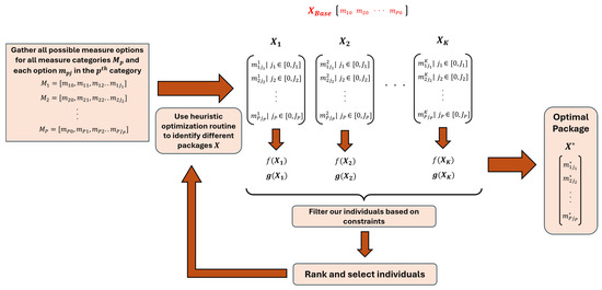
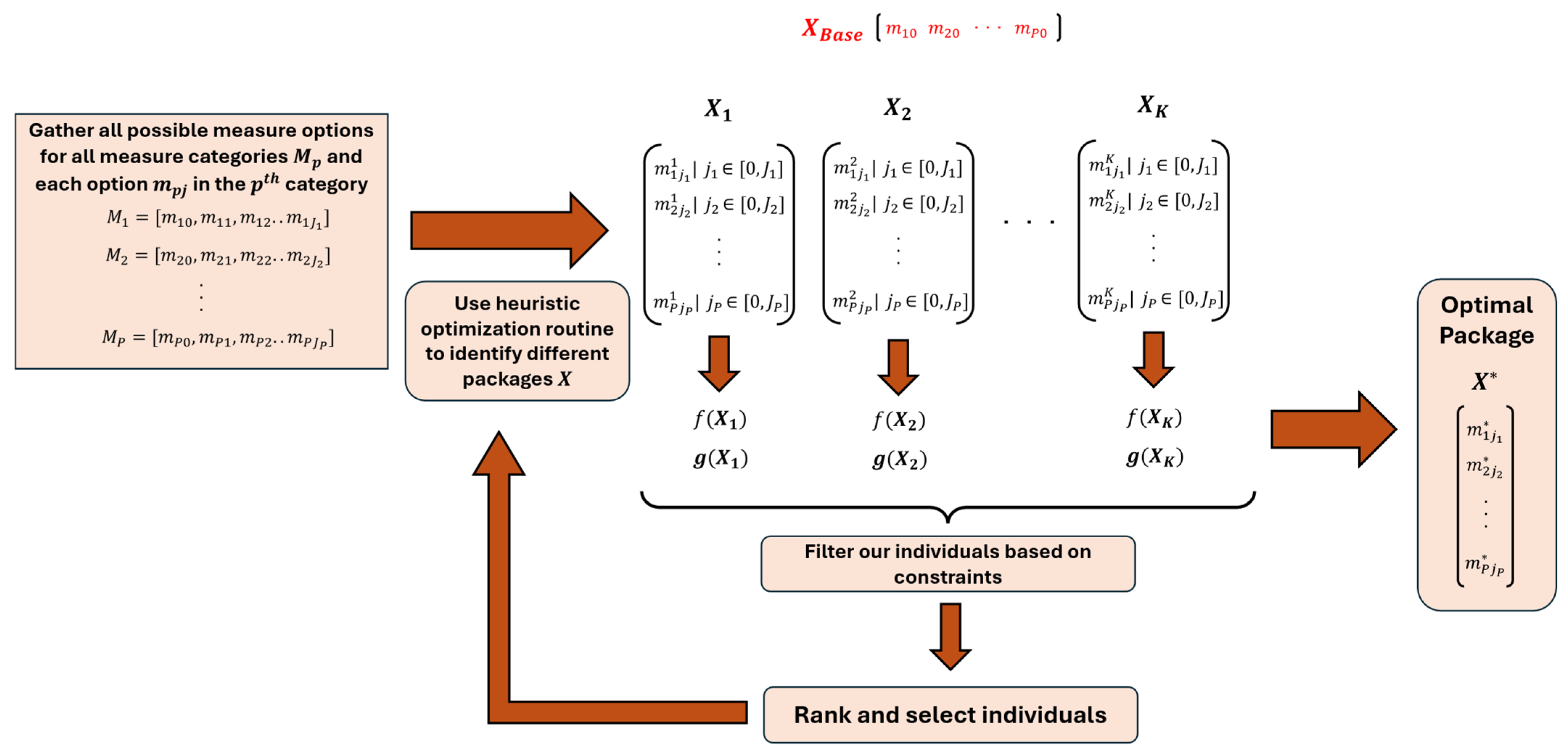
Figure 17 describes the generalized optimization algorithm used to find the best measures package that minimizes a given objective under a set of constraints. First, all possible measure options in each measure category $M_p$ are identified. These options include the baseline represented by index $0$ and the other remaining options going from $1$ to $J_p$. From all existing options, a heuristic optimization method is used to select $K$ individuals, each representing a measures package. Each of the measure packages are evaluated and the values of the objective function $f\left(X\right)$ and constraints $g_i\left(X\right)$ are estimated. All packages that violate the constraints are eliminated. Among the remaining options, a ranking procedure is used to select the best individuals, which are then used to generate a new generation of individuals, each representing a different measures package. This process continues until the value of the objective function does not change significantly. The routine used to select a new generation of individuals can be based on any of the three optimization techniques, including Genetic Algorithm, Particle Swarm Optimization, and sequential search.

Figure 17. Generalized algorithm to identify the most optimal measures package from a given list of individual measures implemented in SABER.

6. Application of SABER to Case Studies

In this section, two case studies are considered to demonstrate and assess the capabilities of SABER to perform energy retrofit analyses for existing residential buildings. Table 6 summarizes the main characteristics of the two single-family homes located in cold-dominated climates.

Table 6. Main characteristics of two different residential building case studies analyzed using SABER.

Case Study	Building A	Building B
Location	Lakewood, CO	Boulder, CO
Floor Area	$1800 \mathrm{s}\mathrm{f}\mathrm{t} \left(167.2 \mathrm{s}\mathrm{q}\mathrm{m}\right)$	$1382 \mathrm{s}\mathrm{f}\mathrm{t} \left(128.4 \mathrm{s}\mathrm{q}\mathrm{m}\right)$
Shape	Rectangle	L-shaped
Orientation	East	Northeast
Floor Quantity	2	1
Exterior Wall Construction	Uninsulated 2 × 4 insulated wood studs with brick finish	2 × 4 insulated wood studs with brick finish and R19 insulation
Exterior Roof Construction	Asphalt shingles with R30 attic insulation	Asphalt shingles with R49 attic insulation
Infiltration Rate	$0.2 \mathrm{A}\mathrm{C}\mathrm{H}$	$0.969 \mathrm{A}\mathrm{C}\mathrm{H}$
Window Material	Single-pane storm windows with metal frames	Double-pane clear windows
WWR	5.1%	14.8%
Lighting Power Density (LPD)	$1.02 \mathrm{W}/\mathrm{s}\mathrm{f}\mathrm{t}$ $(11 \mathrm{W}/\mathrm{s}\mathrm{q}\mathrm{m})$	$0.82 \mathrm{W}/\mathrm{s}\mathrm{f}\mathrm{t}(8.8 \mathrm{W}/\mathrm{s}\mathrm{q}\mathrm{m})$
Equipment Power Density (EPD)	$2 \mathrm{W}/\mathrm{s}\mathrm{f}\mathrm{t} (21 \mathrm{W}/\mathrm{s}\mathrm{q}\mathrm{m})$	$3.74 \mathrm{W}/\mathrm{s}\mathrm{f}\mathrm{t} (40.2 \mathrm{W}/\mathrm{s}\mathrm{q}\mathrm{m})$
Heating Equipment	Forced air gas furnace (AFUE 92%)	Forced air gas furnace (AFUE 80%)
Cooling Equipment	Central air conditioner (SEER 11)	No cooling
DHW Equipment	$40 \mathrm{g}\mathrm{a}\mathrm{l}$ natural gas boiler	$40 \mathrm{gal}$ natural gas boiler
Heating Setpoint	$65 °\mathrm{F} (18.3 °\mathrm{C})$	$70 °\mathrm{F} (21.1 °\mathrm{C})$
Cooling Setpoint	$74 °\mathrm{F} (23.3 °\mathrm{C})$	NA

6.1. Modeling and Calibration

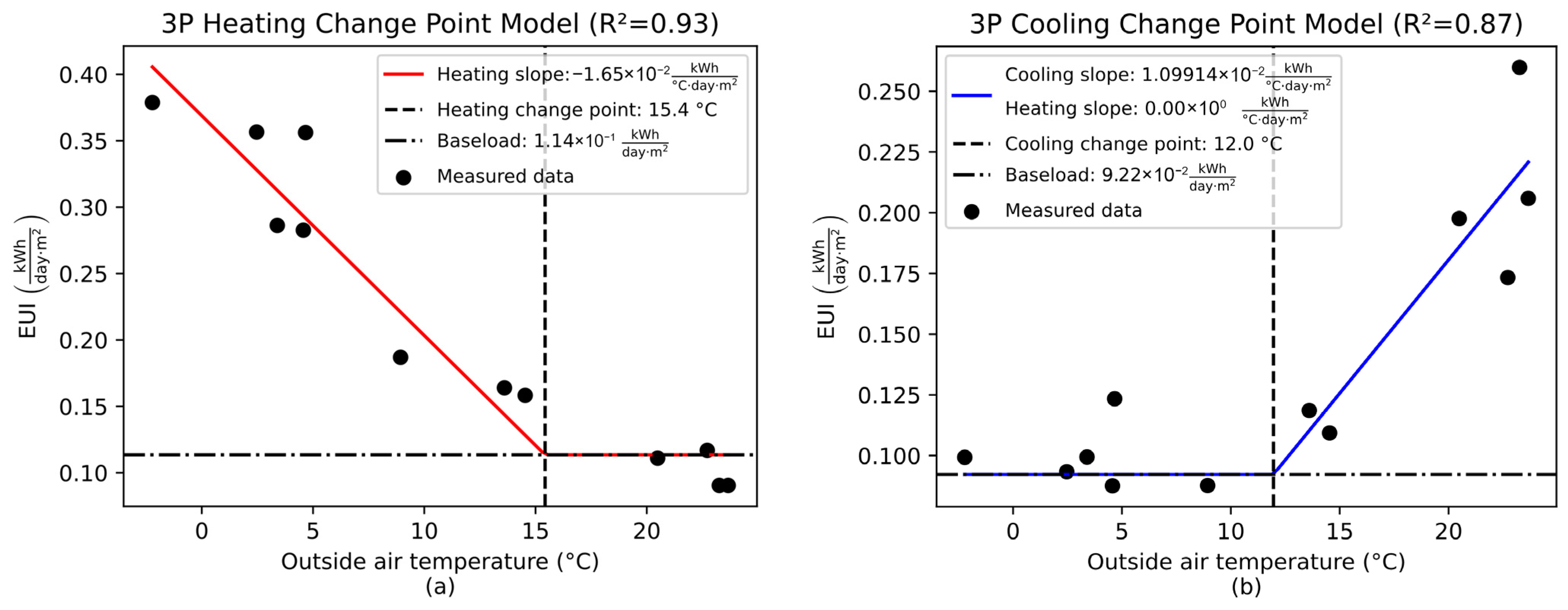
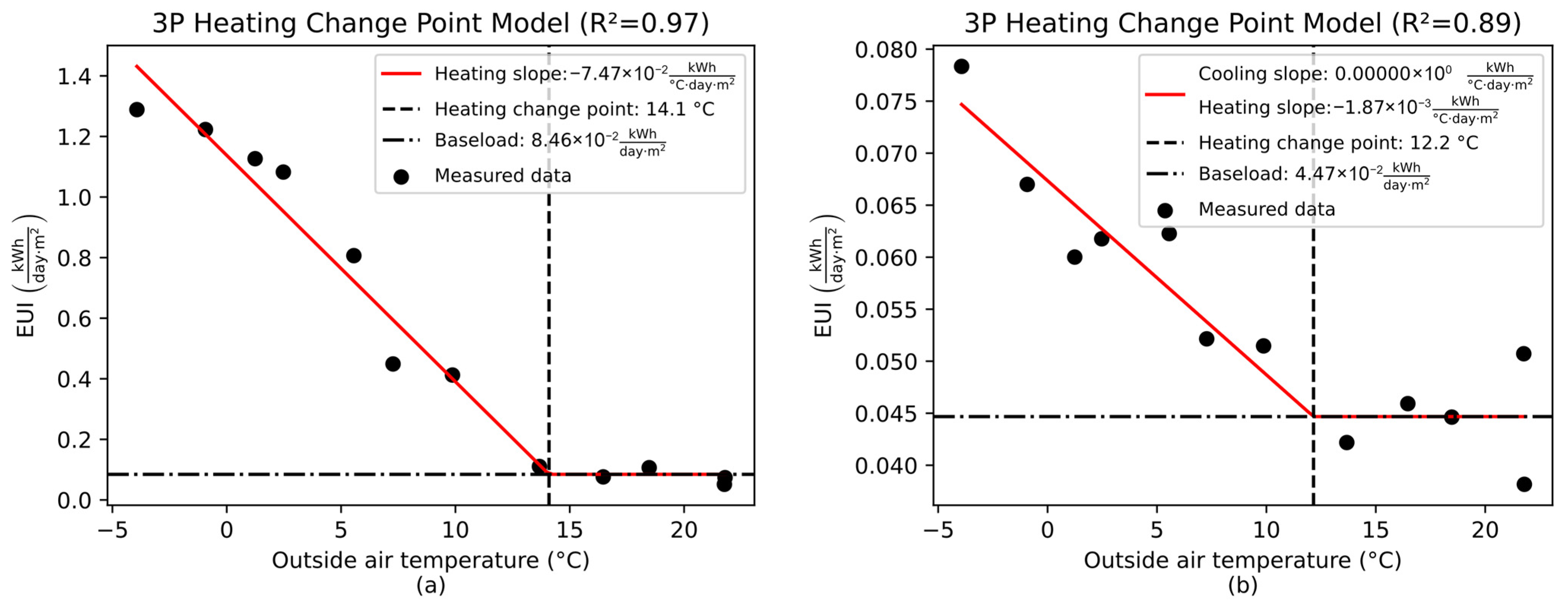
The basic building information outlined in Table 6 is used to develop an energy model for each case study suitable for EnergyPlus using the automatic model creation procedure described in Figure 3. In addition, the monthly utility data is collected for the two sites and processed to calibrate the default schedules used in the EnergyPlus model. First, the change point models are determined for both case studies, as illustrated in Figure 18 and Figure 19 and summarized in Table 7.

Figure 18. Temperature-based change point models for (a) natural gas use and (b) electricity use show obtained energy signature characteristics obtained for Building A.

Figure 19. Temperature-based change point models for (a) natural gas use and (b) electricity use show obtained energy signature characteristics obtained for Building B.

Table 7. Summary of temperature-based change point model parameters obtained by SABER for two case studies.

	Building A		Building B
Utility	Natural Gas	Electricity	Natural Gas	Electricity
Model Type	3P Heating	3P Cooling	3P Heating	3P Heating
Monthly Baseload	$19.4 \mathrm{t}\mathrm{h}\mathrm{e}\mathrm{r}\mathrm{m}\mathrm{s}$	$475 \mathrm{k}\mathrm{W}\mathrm{h}$	$12 \mathrm{t}\mathrm{h}\mathrm{e}\mathrm{r}\mathrm{m}\mathrm{s}$	$170.2 \mathrm{k}\mathrm{W}\mathrm{h}$
Heating Slope	$-162 \mathrm{k}\mathrm{B}\mathrm{t}\mathrm{u}/\mathrm{℉}$ $\left(-85.4 \mathrm{k}\mathrm{W}\mathrm{h}/\mathrm{℃}\right)$	-	$-580.3 \mathrm{k}\mathrm{B}\mathrm{t}\mathrm{u}/\mathrm{℉}$ $\left(-306.1 \mathrm{k}\mathrm{W}\mathrm{h}/\mathrm{℃}\right)$	$-13.6 \mathrm{k}\mathrm{B}\mathrm{t}\mathrm{u}/\mathrm{℉}$ $\left(-7.1 \mathrm{k}\mathrm{W}\mathrm{h}/\mathrm{℃}\right)$
Cooling Slope	-	$102.6 \mathrm{k}\mathrm{B}\mathrm{t}\mathrm{u}/\mathrm{℉}$ $\left(54.1 \mathrm{k}\mathrm{W}\mathrm{h}/\mathrm{℃}\right)$	-	-
Heating Change Point	$59.77 °\mathrm{F}$ $(15.4 °\mathrm{C})$	-	$57.35 °\mathrm{F}$ $(14 °\mathrm{C})$	$53.8 °\mathrm{F}$ $(12.1 °\mathrm{C})$
Cooling Change Point	-	$53.5 °\mathrm{F}$ $(11.9 °\mathrm{C})$	-	-
Model Performance ($R^2)$	$0.925$	$0.752$	$0.94$	$0.9$

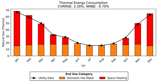
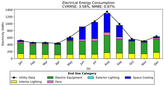
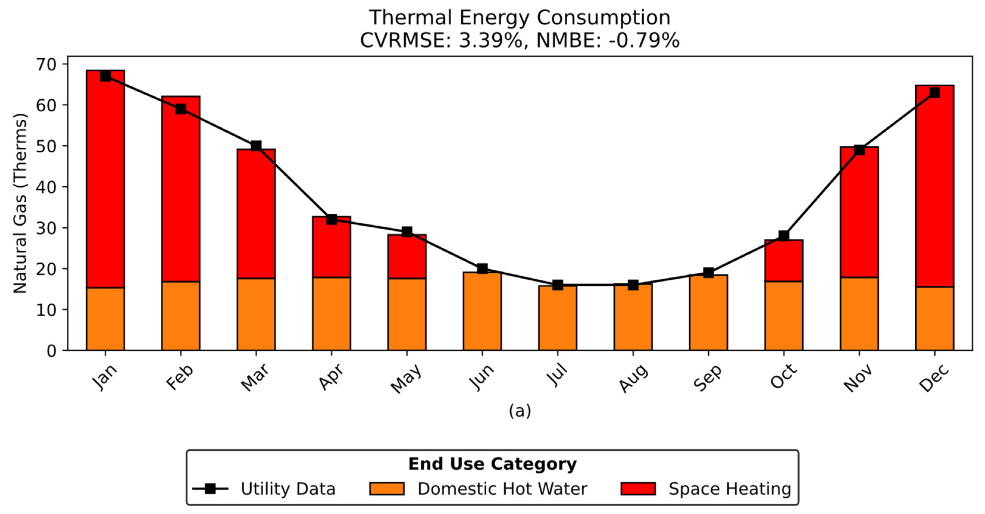
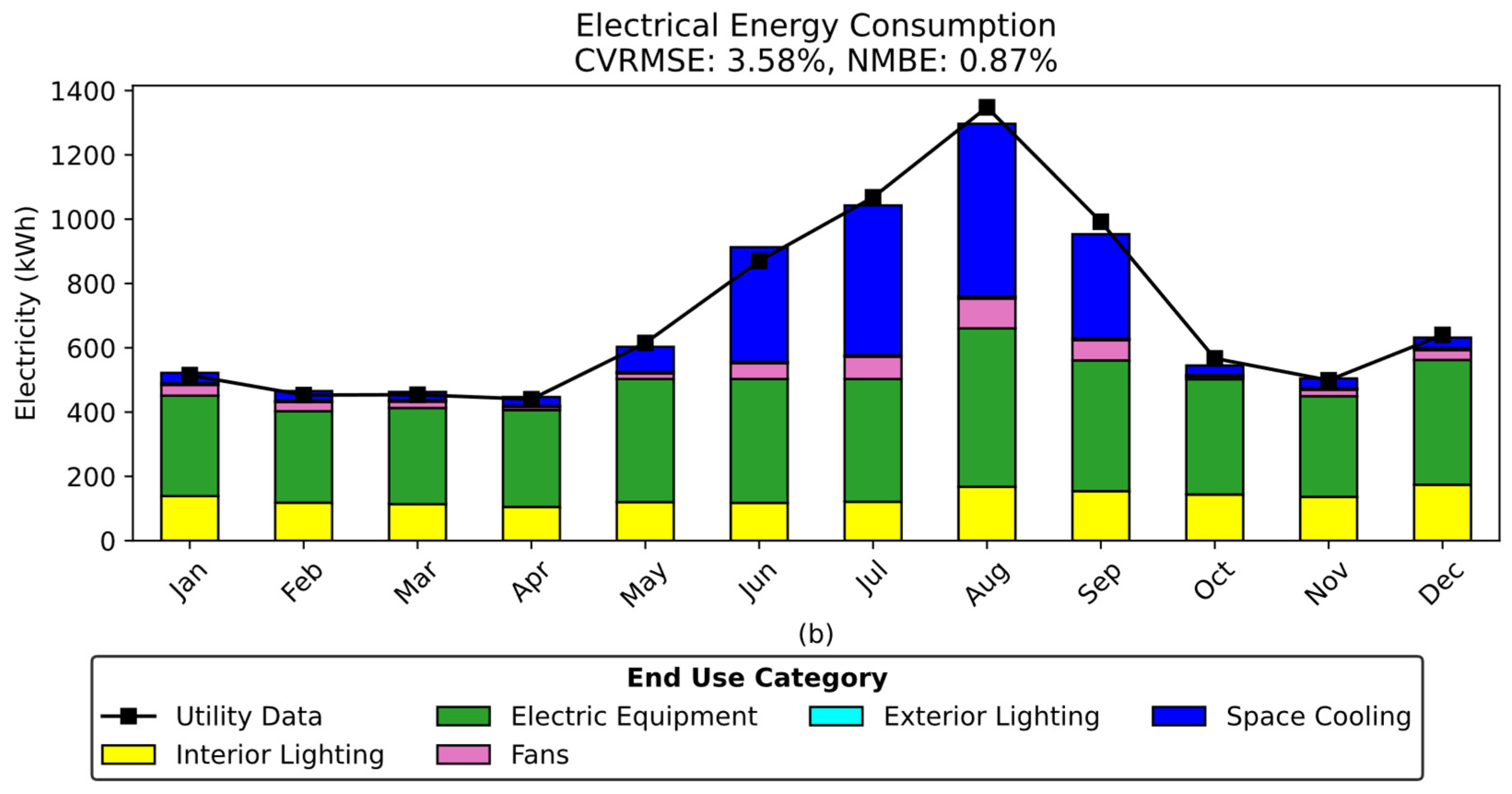
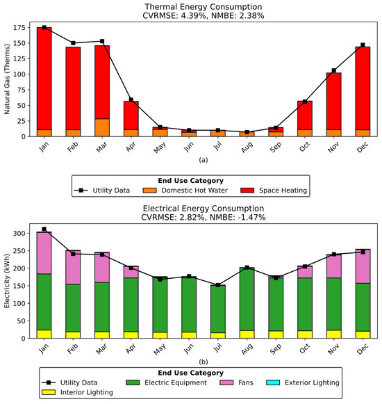
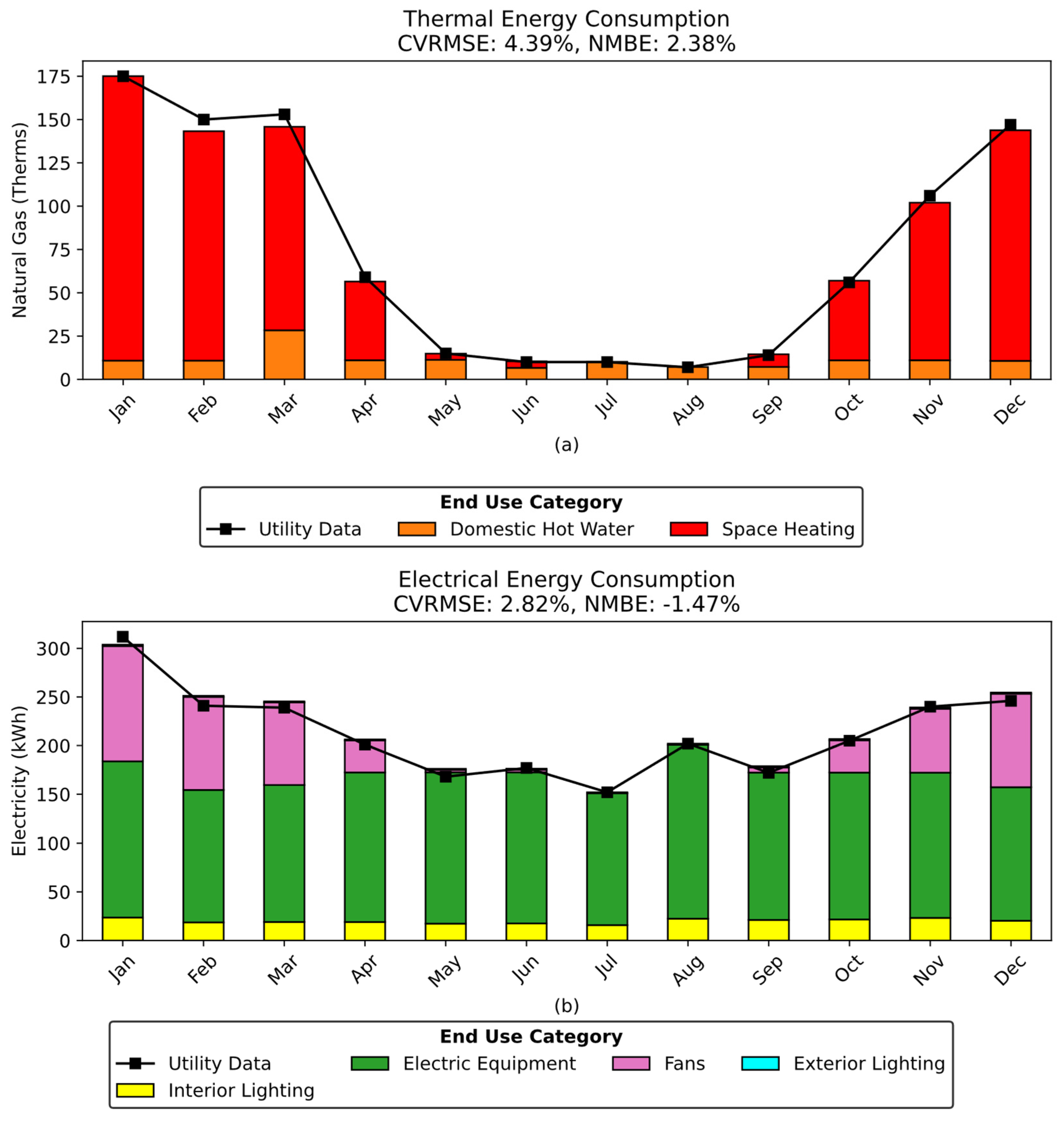
The electricity consumption of Building B, as shown in Figure 19, indicates that there is electricity-based heating but no cooling. The heating electricity consumption is due to the fan being used to drive hot air during the winter season. Using the results of the change point models, detailed building energy models are developed for both homes and are calibrated with the corresponding utility data. Figure 20 and Figure 21 show the monthly energy end-uses obtained from the SABER-calibrated energy models against the utility data. As indicated by the CVRMSE and NMBE values, the monthly electricity and natural gas usages predicted by the SABER-developed models are within the threshold specified by the ASHRAE Guideline 14 requirements [37].

Figure 20. Comparison of monthly energy end-use consumption for (a) natural gas and (b) electricity obtained from SABER-calibrated building model against utility data for Building A.

Figure 21. Comparison of monthly energy end-use consumption for (a) natural gas use and (b) electricity use obtained from the SABER-calibrated building simulation model against the utility data collected from the site for Building B, showing the prediction accuracy of the calibrated model.

6.2. Evaluation of Individual Retrofit Measures

SABER is used to evaluate the impact of retrofit measures for each of the two case studies. The implementation costs of the different measures considered here are summarized in Table 8. Table 9 shows the annual electricity and natural gas energy usages and life cycle costs. The energy and cost benefits estimated by the SABER analysis, using the calibrated energy models for the four measures, are outlined in Table 10 for both building case studies. Here, an electricity utility rate of $\$0.144/\mathrm{k}\mathrm{W}\mathrm{h}$ and a natural gas utility rate of $\$0.944/\mathrm{t}\mathrm{h}\mathrm{e}\mathrm{r}\mathrm{m}(\$0.032/\mathrm{k}\mathrm{W}\mathrm{h})$ are used. For the LCC analysis, a lifetime of $N=15 \mathrm{y}\mathrm{e}\mathrm{a}\mathrm{r}\mathrm{s}$ and a discount rate of $d=5\%$ are considered for the cost benefit analysis carried out by SABER.

Table 8. Summary of implementation costs for four retrofit measures considered in two case studies.

Measure Category	Measure Option	Fixed Cost	Variable Cost per Unit	Measure Unit
Wall Insulation	R36 Spray Foam	$0$	$\$5.69/\mathrm{s}\mathrm{f}\mathrm{t}$ $(\$61.2/\mathrm{s}\mathrm{q}\mathrm{m})$	Exterior Wall Area
Window Material	Low-e Double Pane, Medium SHGC, Argon Filled, Insulated	$0$	$\$35.6/\mathrm{s}\mathrm{f}\mathrm{t}$ $(\$383.2/\mathrm{s}\mathrm{q}\mathrm{m})$	Window Area
Occupancy Sensor Lighting Controls	Yes	$0$	$\$0.12/\mathrm{s}\mathrm{f}\mathrm{t}$ $(\$1.3/\mathrm{s}\mathrm{q}\mathrm{m})$	Floor Area
HVAC Electrification	Heat Pump (HSPF8.8–SEER15)	$\$2856$	$\$42/\mathrm{k}\mathrm{B}\mathrm{t}\mathrm{u}/\mathrm{h}$ $(\$143.3/\mathrm{k}\mathrm{W})$	Main Coil Capacity

Table 9. Annual energy usages and utility costs for two case studies.

Case	Building A	Building B
Total Electricity Consumption	$8387 \mathrm{k}\mathrm{W}\mathrm{h}$	$2593 \mathrm{k}\mathrm{W}\mathrm{h}$
Total Natural Gas Consumption	$451 \mathrm{t}\mathrm{h}\mathrm{e}\mathrm{r}\mathrm{m}\mathrm{s}$	$881 \mathrm{t}\mathrm{h}\mathrm{e}\mathrm{r}\mathrm{m}\mathrm{s}$
Annual Site Energy	$\mathrm{21,617} \mathrm{k}\mathrm{W}\mathrm{h}$	$\mathrm{28,392} \mathrm{k}\mathrm{W}\mathrm{h}$
Annual Source Energy	$\mathrm{40,904} \mathrm{k}\mathrm{W}\mathrm{h}$	$\mathrm{36,178} \mathrm{k}\mathrm{W}\mathrm{h}$
Annual Operation Cost ($)	$\$1628$	$\$1202$
Life Cycle Cost	$\$\mathrm{16,899}$	$\$\mathrm{12,484}$

Table 10. Energy and cost benefits estimated by SABER for four retrofit measures deployed in two case studies.

Property Type	Study	Base Value	New Value	Source Energy Savings (%)	Ratio of Life Cycle Cost with Respect to the Baseline	Simple Payback Period (yrs)
Wall Insulation	Building A	Uninsulated	R36 Spray Foam	8.35%	1.5	81.8
	Building B	R19 Fiberglass	R36 Spray Foam	1.34%	1.55	470.2
Window Material	Building A	Single Pane, Clear	Low-e Double Pane, Medium SHGC, Argon Filled, Insulated	3.19%	1.13	57.7
	Building B	Double Pane, Clear	Low-e Double Pane, Medium SHGC, Argon Filled, Insulated	7.2%	1.68	115.7
Occupancy Sensor Lighting Controls	Building A	No	Yes	3.6%	0.96	3
	Building B	No	Yes	0.6%	1.01	10.8
Heat Pumps	Building A	Gas Furnace (92.5%) Air Conditioner (10 SEER)	Heat Pump (HSPF8.8–SEER15)	3.15%	1.23	−53
	Building B	Gas Furnace (80%)	Heat Pump (HSPF8.8–SEER15)	−15.4%	1.31	−5.4

As noted in Table 10, SABER estimates the annual savings in source energy use and energy cost as well as the life cycle costs and simple payback periods for all the evaluated retrofit measures. For instance, the heat pump retrofit measure, consisting of replacing the existing HVAC system with a heat pump, shows an increase in source energy use compared to the existing situation, which uses gas furnaces for supplying heating to both evaluated buildings. This source energy increase is explained by the relatively high site-to-source conversion of electricity supplied by the grid, estimated at 3.17 for both sites. Further, a life cycle cost ratio of more than one indicates that replacing the HVAC system is not cost-effective using a lifetime of 15 years. The cost-ineffectiveness of retrofitting the gas furnaces with heat pumps in the two considered case studies can be attributed to the low cost of natural gas, set at $\$0.032/\mathrm{k}\mathrm{W}\mathrm{h},$ compared to the electricity rate of $\$0.144/\mathrm{k}\mathrm{W}\mathrm{h}$. Therefore, the results in Table 10 call for the exploration of optimized retrofit packages that include multiple retrofit measures that could make electrification cost-beneficial for the evaluated case studies.

6.3. Evaluation of Optimized Retrofit Measures Package

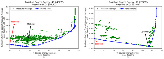
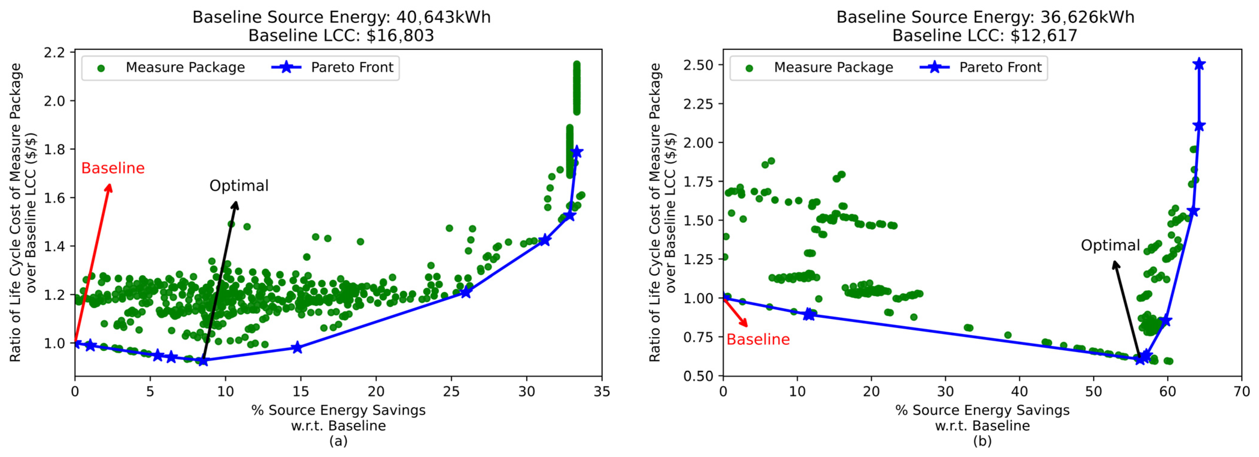
The optimization module in SABER is used to evaluate the optimal combination of individual retrofit measures for both case studies considered in Section 6. The sequential search technique is used to identify the best combination of retrofit measures that can minimize the life cycle costs while maximizing the annual source energy use savings. Figure 22 illustrates the Pareto front obtained for both case study buildings, along with the other sub-optimal retrofit packages.

Figure 22. Results of sequential search optimization technique for (a) Building A and (b) Building B, showing the search path for reaching the optimal solution.

For both case studies, the Pareto fronts exhibit retrofit packages with minimum life cycle costs. Table 11 summarizes the lists of measures and their energy and cost benefits for the optimal packages identified by SABER for the two case studies.

Table 11. Impact of individual measures and combined measures package for different case studies for the optimal package obtained using sequential search.

Case Study	Measure	% Source Energy Savings	% Change in Annual Operating Cost	Ratio of LCC w.r.t. Baseline	Simple Payback Period (yrs)
Building A	Optimal Package	8.5%	9.9%	0.92	2.8
	Implement daylighting sensor control	1.01%	1.2%	0.98	1.11
	Change all existing lighting fixtures to LEDs	4.88%	5.9%	0.95	2.26
	Implement a night setback of 2C	0.88%	0.7%	0.99	-
	Implement occupancy sensor controls	3.89%	4.7%	0.96	2.83
Building B	Optimal Package	56.2%	52.3%	0.6	2.55
	Implement a night setback of 10C	10.5%	9.7%	0.9	-
	Implement daylighting sensor controls	0.31	0.46%	0.99	4.3
	Reduce infiltration rate from 0.96ACH to 0.1ACH	53.6%	49.7%	0.65	3.18

For each of the measures there is a reduction in consumption of electricity and natural gas and a similar reduction in energy costs. Table 11 indicates that the optimized retrofit packages are highly cost-effective, with payback periods of less than 3 years. Moreover, the results listed in Table 11 allow us to assess the level of the interactive effects among the different measures for both optimized retrofit packages. For instance, the sum of source energy savings of the individual measures for Building B is estimated to be 64.4%, whereas the associated optimal package shows source savings of only 56.2%. The difference in these results confirms that the summation of individual measures tends to overestimate the total amount of savings, which can be avoided by SABER considering all of them together.

7. Summary and Conclusions

A new retrofit audit tool for buildings, referred to as the Simplified and Automated Building Energy Retrofit analysis tool or SABER, is described and demonstrated in this paper. The tool has an easy-to-use intuitive graphical user interface and provides four main functionalities: (i) create, from basic user input data, a detailed EnergyPlus building energy model; (ii) conduct an effective calibration of the building energy model using monthly utility data; (iii) perform energy and cost benefit analyses of individual and packaged retrofit measures; and (iv) optimize the selection of retrofit measures to minimize the life cycle costs and maximize energy savings.

The capabilities of the tool are verified and demonstrated using various case studies. The results of both the verification analysis and the demonstrated case studies confirm that SABER is able to develop well-calibrated energy models for existing buildings. Moreover, the tool can effectively handle the interactive effects of various retrofit measures and thus more accurately assess the energy and cost benefits of any given retrofit measures package. Finally, SABER is shown to be capable of performing optimized retrofit analyses and identifying the best retrofit set of energy efficiency measures that minimize the life cycle costs.

SABER is currently limited to generating a single-zone model of a building in EnergyPlus. Although this method is best suited for residential buildings, SABER could potentially be used to model any building typology upon the expansion of the existing HVAC equipment templates and inclusion of diverse operation schedules. Further, to maintain its user-friendliness and broad accessibility, SABER limits itself to building calibration models using monthly utility data only.

The tool is also being prepared for deployment as an online platform for testing and use by the academic community. Although SABER currently supports only rectangular and L-shaped building geometries with a limited set of wall and roof assemblies and HVAC system types, its flexible approach allows for easy expansion of its capabilities. In addition, future work will explore the use of machine learning-based methods for energy signature analysis and unknown parameter estimation using hourly measured data. Moreover, future work could expand SABER to select retrofit measures under uncertain conditions using sophisticated optimization methods to satisfy a range of objectives, like cost and carbon emissions, under constraints such as limited retrofit budgets, acceptable thermal comfort levels, and desired electrical panel capacities.

The primary strength of SABER is its integration of different functionalities required for a detailed retrofit analysis into a single tool. Thus, SABER has significant benefits compared to existing tools for automating whole-building energy modeling and calibration to facilitate retrofit analysis of existing buildings. Future enhancements of SABER will include the incorporation of input parameter identification during the calibration process for cases where the physical features of existing buildings are difficult to obtain. Moreover, other optimization cost functions and constraints will be integrated in the tool to consider non-energy benefits and the space and budgetary limitations of retrofit analyses.

References

- IEA. Sustainable Recovery; IEA: Paris, France, 2020; Available online: https://www.iea.org/reports/sustainable-recovery (accessed on 9 April 2026).
- Zhou, Z.; Zhang, S.; Wang, C.; Zuo, J.; He, Q.; Rameezdeen, R. Achieving energy efficient buildings via retrofitting of existing buildings: A case study. J. Clean. Prod. 2016, 112, 3605–3615. [Google Scholar] [CrossRef] [Scilit]
- Dall’O’, G.; Galante, A.; Pasetti, G. A methodology for evaluating the potential energy savings of retrofitting residential building stocks. Sustain. Cities Soc. 2012, 4, 12–21. [Google Scholar] [CrossRef] [Scilit]
- Liang, J.; Qiu, Y.; James, T.; Ruddell, B.L.; Dalrymple, M.; Earl, S.; Castelazo, A. Do energy retrofits work? Evidence from commercial and residential buildings in Phoenix. J. Environ. Econ. Manag. 2018, 92, 726–743. [Google Scholar] [CrossRef] [Scilit]
- Cohen, S.; Goldman, C.; Harris, J. Energy savings and economics of retrofitting single-family buildings. Energy Build. 1991, 17, 297–311. [Google Scholar] [CrossRef] [Scilit]
- Giandomenico, L.; Papineau, M.; Rivers, N. A Systematic Review of Energy Efficiency Home Retrofit Evaluation Studies. Annu. Rev. Resour. Econ. 2022, 14, 689–708. [Google Scholar] [CrossRef] [Scilit]
- Bouckaert, S.; Pales, A.F.; McGlade, C.; Remme, U.; Wanner, B.; Varro, L.; D’Ambrosio, D.; Spencer, T. Net Zero by 2050: A Roadmap for the Global Energy Sector. 2021. Available online: https://www.iea.org/reports/net-zero-by-2050 (accessed on 9 April 2026).
- IEA. Renovation of Near 20% of Existing Building Stock to Zero-Carbon-Ready by 2030 Is Ambitious But Necessary; IEA: Paris, France, 2022; Available online: https://www.iea.org/reports/renovation-of-near-20-of-existing-building-stock-to-zero-carbon-ready-by-2030-is-ambitious-but-necessary (accessed on 4 April 2026).
- Pérez-Navarro, J.; Bueso, M.C.; Vázquez, G. Drivers of and Barriers to Energy Renovation in Residential Buildings in Spain—The Challenge of Next Generation EU Funds for Existing Buildings. Buildings 2023, 13, 1817. [Google Scholar] [CrossRef] [Scilit]
- O’Malley, E.; Scott, S.; Sorrell, S. Barriers to Energy Efficiency: Evidence from Selected Sectors. Res. Ser. 2003, PRS47. Available online: https://ideas.repec.org//b/esr/resser/prs47.html (accessed on 18 November 2025).
- Gonzalez-Caceres, A.; Rabani, M.; Wegertseder Martínez, P.A. A systematic review of retrofitting tools for residential buildings. IOP Conf. Ser. Earth Environ. Sci. 2019, 294, 012035. [Google Scholar] [CrossRef] [Scilit]
- Seddiki, M.; Bennadji, A.; Laing, R.; Gray, D.; Alabid, J.M. Review of Existing Energy Retrofit Decision Tools for Homeowners. Sustainability 2021, 13, 10189. [Google Scholar] [CrossRef] [Scilit]
- ANSI/ASHRAE/IES 211-2018; Standard Practice for Inspection and Maintenance of Commercial Building HVAC Systems. ANSI/ASHRAE/IES: Peachtree Corners, GA, USA, 2018.
- “EnergyPlusTM,” National Renewable Energy Laboratory (NREL), Golden, CO (United States); Lawrence Berkeley National Laboratory (LBNL), Berkeley, CA (United States), EnergyPlusTM (e+); 005462MLTPL00, September 2017. Available online: https://www.osti.gov/biblio/1395882 (accessed on 6 July 2023).
- eQUEST. Available online: https://www.doe2.com/equest/ (accessed on 18 November 2025).
- Qu, K.; Chen, X.; Ekambaram, A.; Cui, Y.; Gan, G.; Økland, A.; Riffat, S. A novel holistic EPC related retrofit approach for residential apartment building renovation in Norway. Sustain. Cities Soc. 2020, 54, 101975. [Google Scholar] [CrossRef] [Scilit]
- Lee, S.H.; Hong, T.; Piette, M.A.; Taylor-Lange, S.C. Energy retrofit analysis toolkits for commercial buildings: A review. Energy 2015, 89, 1087–1100. [Google Scholar] [CrossRef] [Scilit]
- Forouzandeh, N.; Tahsildoost, M.; Zomorodian, Z.S. A review of web-based building energy analysis applications. J. Clean. Prod. 2021, 306, 127251. [Google Scholar] [CrossRef] [Scilit]
- Szum, C.; Li, H.; Snyder, S.C.; Bekhit, A.; Nesler, C.G.; Lisauskas, S. Building Efficiency Targeting Tool for Energy Retrofits (BETTER) Analytical Engine; Lawrence Berkeley National Laboratory (LBNL): Berkeley, CA, USA, 2018.
- U.S. Environmental Protection Agency. ENERGY STAR Portfolio Manager. Available online: https://www.energystar.gov/portfoliomanager (accessed on 20 February 2026).
- Green Upgrade Calculator. Rocky Mountain Institute (RMI). Web Application. Available online: https://greenup.rmi.org/ (accessed on 19 September 2025).
- Wang, N.; Gorrissen, W.J. Commercial Building Energy Asset Score System: Program Overview and Technical Protocol (Version 1.0); PNNL—22045; Pacific Northwest National Laboratory (PNNL): Richland, WA, USA, 2012.
- Hong, T.; Piette, M.A.; Chen, Y.; Lee, S.H.; Taylor-Lange, S.C.; Zhang, R.; Sun, K.; Price, P. Commercial Building Energy Saver: An energy retrofit analysis toolkit. Appl. Energy 2015, 159, 298–309. [Google Scholar] [CrossRef] [Scilit]
- Sun, K.; Hong, T.; Taylor-Lange, S.C.; Piette, M.A. A pattern-based automated approach to building energy model calibration. Appl. Energy 2016, 165, 214–224. [Google Scholar] [CrossRef] [Scilit]
- Weatherization Assistant. Available online: https://weatherization.ornl.gov/softwaredescription/ (accessed on 14 October 2025).
- Macumber, D.; Parker, A.; Lisell, L.; Metzger, I.; Brown, M. Simuwatt—A Tablet Based Electronic Auditing Tool; International Building Performance Simulation Association (IBPSA), NREL/CP-5500-61418, May 2014. Available online: https://www.osti.gov/biblio/1274097 (accessed on 14 October 2025).
- How It Works | Buildee. Available online: https://buildee.com/how-it-works/ (accessed on 14 October 2025).
- Title 24 Nonresidential Compliance Software. Available online: https://bees.noresco.com/index.html (accessed on 14 October 2025).
- Kesik, T.; Lio, M.; Associates, D. HOT2.XP: Energuide for Houses and the New Housing Market, Presented at the eSim 2001, in eSim, Vol. 1. IBPSA-Canada, 2001. Available online: https://publications.ibpsa.org/conference/paper/?id=esim2001_14 (accessed on 14 October 2025).
- Canada, N.R. HOT2XP. Available online: https://natural-resources.canada.ca/science-data/data-analysis/geospatial-data-tools-services/hot2xp (accessed on 14 October 2025).
- Christensen, C.; Anderson, R.; Horowitz, S.; Courtney, A.; Spencer, J. BEopt(TM) Software for Building Energy Optimization: Features and Capabilities; National Renewable Energy Laboratory: Golden, CO, USA, 2006. [CrossRef] [Scilit]
- Chen, Y.; Hong, T.; Piette, M.A. Automatic generation and simulation of urban building energy models based on city datasets for city-scale building retrofit analysis. Appl. Energy 2017, 205, 323–335. [Google Scholar] [CrossRef] [Scilit]
- Xero Home App. Available online: https://xerohome.com/app/#/ (accessed on 14 October 2025).
- Starke, A.; Willemsen, M.; Snijders, C. Effective User Interface Designs to Increase Energy-efficient Behavior in a Rasch-based Energy Recommender System. In Proceedings of the Eleventh ACM Conference on Recommender Systems in RecSys ’17; Association for Computing Machinery: New York, NY, USA, 2017; pp. 65–73. [Google Scholar]
- Adan, H.; Fuerst, F. Do energy efficiency measures really reduce household energy consumption? A difference-in-difference analysis. Energy Effic. 2016, 9, 1207–1219. [Google Scholar] [CrossRef] [Scilit]
- Christensen, C. A Sequential Search Technique for Identifying Optimal Building Designs on the Path to Zero Energy Buildings. In Proceedings of the Solar Conference, Portland, OR, USA, 11–14 July 2004; Available online: https://www.academia.edu/125086921/A_Sequential_Search_Technique_for_Identifying_Optimal_Building_Designs_on_the_Path_to_Zero_Energy_Buildings (accessed on 21 September 2025).
- ASHRAE. Guideline 14-2023: Measurement of Energy, Demand, and Water Savings; American Society of Heating, Refrigerating and Air-Conditioning Engineers: Atlanta, GA, USA, 2023. [Google Scholar]
- Kissock, J.K.; Haberl, J.S.; Claridge, D.E. Inverse Modeling Toolkit: Numerical Algorithms. ASHRAE Trans. 2003, 109, 425–434. [Google Scholar]
- American Society of Heating, Refrigerating and Air-Conditioning Engineers. 2021 ASHRAE Handbook Fundamentals (SI Edition); American Society of Heating Refrigerating and Air-Conditioning Engineers Inc.: Peachtree Corners, GA, USA, 2021. [Google Scholar]
- Kim, K.H.; Haberl, J.S. Development of methodology for calibrated simulation in single-family residential buildings using three-parameter change-point regression model. Energy Build. 2015, 99, 140–152. [Google Scholar] [CrossRef] [Scilit]
- Kim, K.H.; Haberl, J.S. Development of a home energy audit methodology for determining energy-efficient, cost-effective measures in existing single-family houses using an easy-to-use simulation. Build. Simul. 2015, 8, 515–528. [Google Scholar] [CrossRef] [Scilit]
- Krarti, M. Energy Audit of Building Systems: An Engineering Approach, Second Edition, 2nd ed.; CRC Press: Boca Raton, FL, USA, 2016; ISBN 978-0-429-19637-9. [Google Scholar]
- Siddharth, V.; Ramakrishna, P.V.; Geetha, T.; Sivasubramaniam, A. Automatic generation of energy conservation measures in buildings using genetic algorithms. Energy Build. 2011, 43, 2718–2726. [Google Scholar] [CrossRef] [Scilit]
- Tuhus-Dubrow, D.; Krarti, M. Comparative Analysis of Optimization Approaches to Design Building Envelope for Residential Buildings. ASHRAE Trans. 2009, 115, 554–562. [Google Scholar]
- Delgarm, N.; Sajadi, B.; Kowsary, F.; Delgarm, S. Multi-objective optimization of the building energy performance: A simulation-based approach by means of particle swarm optimization (PSO). Appl. Energy 2016, 170, 293–303. [Google Scholar] [CrossRef] [Scilit]
Disclaimer/Publisher’s Note: The statements, opinions and data contained in all publications are solely those of the individual author(s) and contributor(s) and not of MDPI and/or the editor(s). MDPI and/or the editor(s) disclaim responsibility for any injury to people or property resulting from any ideas, methods, instructions or products referred to in the content. |
© 2026 by the authors. Licensee MDPI, Basel, Switzerland. This article is an open access article distributed under the terms and conditions of the Creative Commons Attribution (CC BY) license.