Coordinated Planning of Unbalanced Flexible Interconnected Distribution Networks Based on Distributed Optimization

Abstract

Rapid increases in distributed photovoltaic (PV) penetration have brought additional challenges to distribution network planning and operation. Meanwhile, flexible interconnection devices such as soft open point integrated with battery energy storage system (E-SOP) can significantly enhance the regulatory capability and operational adaptability of the distribution system and have been widely applied in recent years. First, to improve both economic performance and voltage quality, a coordinated planning method for the multi-region flexible interconnected distribution system based on E-SOP is proposed. Second, with the ongoing growth of interconnected distribution networks, centralized optimization methods exhibit limitations in computational efficiency and privacy protection. To address this, the planning model is decomposed into several subproblems by applying the Alternating Direction Method of Multipliers (ADMM), allowing each region to optimize its local subproblem in a fully distributed manner. Additionally, a Shapley value-based cost allocation mechanism is applied to ensure fair and rational cost distribution among different distribution networks. Finally, case studies are conducted to validate the effectiveness of the proposed method. Case studies show that the proposed method reduces the system’s total annual cost by 14.90% and the electricity purchase cost by 28.61% compared with the pre-planning case. Meanwhile, the maximum voltage imbalance is reduced to within the standard range. These results validate the effectiveness of the proposed method in enhancing both economic efficiency and power quality for flexible interconnected distribution systems.

1. Introduction

Renewable energy sources are abundant, secure, and environmentally friendly and have experienced rapid development worldwide in recent years. It is foreseeable that the large-scale grid integration of high-penetration renewable distributed generations (DGs) such as photovoltaic (PV) will become an inevitable trend and a key characteristic of future distribution networks. However, the integration of DGs significantly alters power flow patterns, rendering the planning and operation of distribution systems more complex and technically challenging [1,2,3]. Concurrently, a large number of single-phase loads and asymmetric line parameters often result in three-phase imbalance in distribution networks, which increases system operating losses and adversely affects the safe operation of distribution equipment [4,5]. Studies have shown that a 3% voltage imbalance can increase motor losses by approximately 9% and reduce the service life of the windings to about one-quarter of their expected lifespan [6,7]. Under such circumstances, traditional regulation methods such as transformer tap changing, switching of capacitor banks, and network reconfiguration exhibit slow response and insufficient control precision and are increasingly unable to meet the operational requirements of modern distribution networks [8,9,10,11].

Advances in high-performance power electronic devices, exemplified by soft open point (SOP), provide effective solutions to these challenges. As fully controllable power electronic components, soft open point serves as an alternative to traditional sectionalizing and tie switches, enabling connection between different feeders in distribution networks. Through voltage source converter (VSC) port power control, SOP facilitates power flow redistribution between different feeders, achieving flexible closed-loop operation of distribution systems [12]. Furthermore, SOP can be configured as multi-terminal devices by integrating multiple voltage source converters with a shared DC bus, enabling active power flow management across multiple feeders. Compared with conventional mechanical switches, SOP features an unlimited number of state changes, possesses reactive power compensation capability, and allows independent and continuous control of three-phase power, thus effectively mitigating the problem of insufficient power flow regulation capability in distribution systems. Consequently, investigating the planning of flexible interconnected distribution networks based on SOP is of considerable significance. Currently, several researchers have investigated the planning of SOP in distribution networks. References [13,14,15] considered the impact of DG on system operation and optimized the siting and sizing of SOP accordingly. Distributed renewable energy (DRE) and load uncertainties were considered in [16], where an SOP optimal placement model was proposed to improve three-phase imbalance in distribution networks. In [17], a multi-terminal SOP siting and sizing strategy was proposed to meet the requirements for flexible interconnection of multiple distribution substations under rapid load growth and high-penetration DG integration. In terms of engineering applications, industrial projects of SOP have already been implemented worldwide, including the “Flexible Urban Network—Low Voltage” project in the UK [18], the four-port SOP project in Suzhou, China [19], ABB’s “Mackinac HVDC Flow-Control” project in the US [20], and the “REEL Chapelle-sur-Moudon” project in Switzerland [21].

To enhance equipment flexibility and utilization efficiency, some studies have proposed integrating a battery energy storage (BES) system with the DC port of SOP, forming the soft open point integrated with the battery energy storage system (E-SOP). Through E-SOP, the power released or absorbed by the BES can be flexibly distributed across different feeders, enabling shared utilization of battery energy storage resources among multiple regions. From an operational perspective, E-SOP not only achieves dynamic power allocation between feeders or substations but also provides functionalities including smoothing power fluctuations, peak shaving and valley filling. These capabilities significantly enhance the flexibility of SOP control and play an important role in facilitating renewable energy integration and improving distribution network operational efficiency. In terms of economy, the coordinated construction mode combining SOP with BES improves equipment utilization rates compared to standalone installations and reduces the integrated system operational costs. A multi-stage expansion planning method for E-SOP considering tie-line reconfiguration was proposed in [22], which significantly improved equipment utilization efficiency and the cost-effectiveness of distribution network planning. Reference [23] studied the coordinated planning of multi-port SOP and energy storage, demonstrating that their joint deployment can enhance the hosting capacity of distribution networks and improve operational efficiency while satisfying expected cost-effectiveness.

The existing literature typically limits the planning of SOP and battery energy storage systems to a single investment entity. Under this independent construction and operation paradigm, SOP and energy storage face challenges in cost and fail to fully exploit the value of resources, making it difficult to achieve aggregation effects and leverage cluster support capabilities. In contrast, a multi-stakeholder co-construction and sharing investment and operation model for E-SOP can strengthen inter-cluster energy exchange by sharing flexibility resources, improve the utilization efficiency of SOP and energy storage, and enhance the economic performance of system operation. Furthermore, existing studies generally adopt centralized methods to solve multi-region coordinated planning problems, whereby an individual distribution network uploads internal data to a central system that makes unified planning decisions [24]. However, as the scale of the flexible interconnected distribution system continues to grow, centralized approaches face critical challenges. First, the massive data transmission required in centralized computation increases communication burdens and is constrained by communication bandwidth limits. Second, the expansion of system scale significantly increases the computational difficulty of centralized solvers, resulting in decreased solution efficiency and reduced applicability. Moreover, centralized approaches require sharing internal operational data from each distribution network, which makes it difficult to meet the data privacy and information security requirements of different stakeholders. In contrast, distributed optimization methods such as the Alternating Direction Method of Multipliers (ADMM) allow each distribution network to independently solve its local planning subproblem while only exchanging a small amount of interaction information to achieve global optimization. Such methods exhibit high computational efficiency and strong confidentiality of information [25]. However, the existing literature primarily focuses on applying ADMM to power system operational scheduling problems, with limited exploration of its application to power system planning problems [26,27,28]. Therefore, further research is needed on ADMM-based distributed planning methods for multi-region flexible interconnected distribution system.

Table 1 summarizes the key characteristics of representative studies on SOP planning in distribution networks, including the optimization methods employed and whether factors such as three-phase imbalance, multi-area coordination, energy storage integration, and benefit allocation were considered. As shown in the table, most existing works adopt centralized optimization, overlook unbalanced operation, and focus on single-region planning. Moreover, the integration of distributed optimization with shared energy storage and cost allocation remains largely unexplored. Based on the above comparison, the main research gap lies in the lack of a coordinated planning framework that simultaneously addresses three-phase unbalanced operation, multi-region coupling, distributed solution, energy storage integration, and fair benefit distribution. To fill this gap, this paper develops a distributed planning model for unbalanced flexible interconnected distribution networks, solves it using an improved ADMM algorithm, and allocates the resulting costs through a Shapley value-based mechanism. As a result, the main contributions of this research are as follows:

(1)

A coordinated planning model for multi-region flexible interconnected distribution networks that integrate PV, multi-terminal SOP, and shared energy storage. Unlike existing works that treat SOP and BES separately or limit planning to a single network, the proposed model enables joint investment and operation across regions, thereby improving economic efficiency and voltage quality.

(2)

A fully distributed solution framework based on an improved ADMM algorithm with an adaptive penalty factor update strategy. Compared to centralized methods, the proposed approach preserves the privacy of each distribution network’s internal data and reduces communication burdens. Compared to standard ADMM, it achieves faster convergence and higher solution accuracy.

(3)

A fair cost allocation mechanism using the Shapley value to apportion the total cost among multiple stakeholders. This ensures that each distribution network benefits from cooperation, enhancing the willingness to participate in co-construction and sharing of flexibility resources.

Table 1. Comparison of the existing literature and this study.

Ref.	Optimization Method	Three-Phase Unbalance	Multi-Region	Energy Storage Integration	Benefit Distribution	Main Limitation
[13,14]	Centralized	No	No	No	-	No three-phase unbalance model or energy storage coordination.
[15,22,23]	Centralized	No	No	Yes	-	No unbalance model or multi-region coordination.
[16]	Centralized	Yes	Yes	No	No	Centralized model; no energy storage integration.
[17,24]	Centralized	No	Yes	No	No	No distributed optimization or benefit allocation.
This study	Distributed	Yes	Yes	Yes	Yes	-

Table 1. Comparison of the existing literature and this study.

Ref.	Optimization Method	Three-Phase Unbalance	Multi-Region	Energy Storage Integration	Benefit Distribution	Main Limitation
[13,14]	Centralized	No	No	No	-	No three-phase unbalance model or energy storage coordination.
[15,22,23]	Centralized	No	No	Yes	-	No unbalance model or multi-region coordination.
[16]	Centralized	Yes	Yes	No	No	Centralized model; no energy storage integration.
[17,24]	Centralized	No	Yes	No	No	No distributed optimization or benefit allocation.
This study	Distributed	Yes	Yes	Yes	Yes	-

2. Coordinated Planning Model for Flexible Interconnected Distribution Networks

2.1. Flexible Interconnected Distribution Networks Based on E-SOP

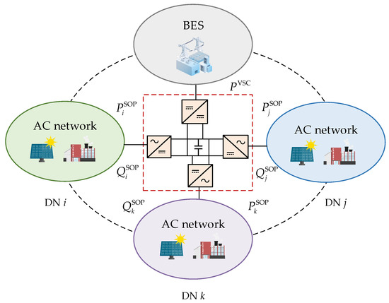
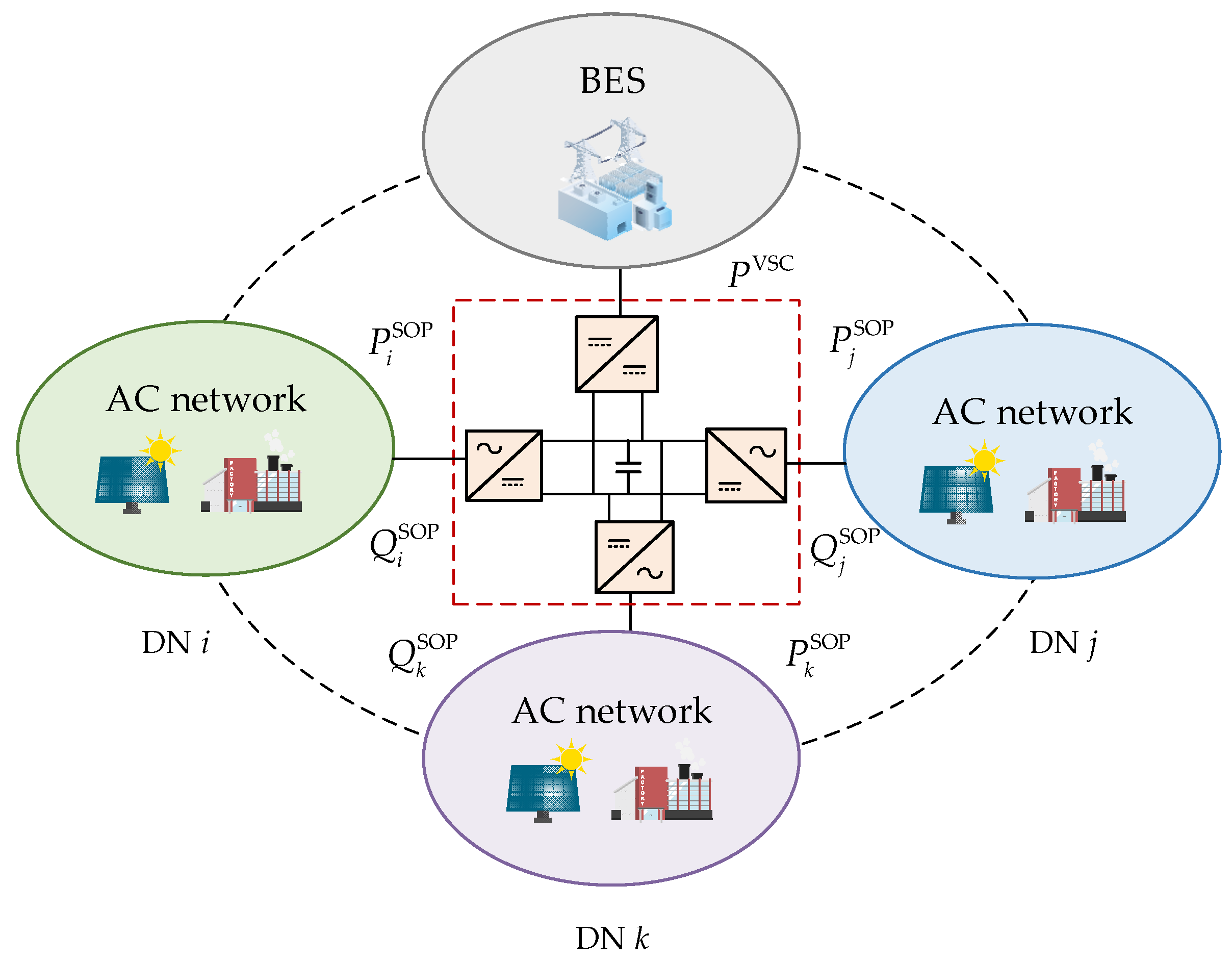
This paper investigates the flexible interconnected distribution system based on E-SOP, with its topological structure illustrated in Figure 1. Regional interconnection and energy exchange between distribution networks are achieved through SOP. By integrating an energy storage unit, SOP is endowed with an energy storage capability in addition to its original power transfer function. As a result, an interconnected distribution system with high operational flexibility is formed.

Figure 1. Flexible interconnected distribution system based on E-SOP.

The E-SOP in the flexible interconnected distribution system is capable of precisely controlling the active and reactive power of every port. However, it must satisfy the active power balance constraint during operation. The reactive power outputs of individual converters, due to DC isolation, do not interfere with each other and can be independently controlled. Furthermore, due to conduction and various switching losses of semiconductor devices, non-negligible power losses occur during E-SOP operation, which must be incorporated into the optimization framework. This leads to the formulation of the E-SOP optimization model, with the following constraints:

$$\sqrt{{\left(P_{i,s,t}^{\mathrm{SOP},\phi }\right)}^2+{\left(Q_{i,s,t}^{\mathrm{SOP},\phi }\right)}^2}\le S_{i,\phi ,\mathrm{SOP}}$$

(1)

$${\displaystyle \sum _{i\in {\mathsf{\Omega }}_{\mathrm{SOP}}}{\displaystyle \sum _{\phi \in \left\{a,b,c\right\}}\left(P_{i,s,t}^{\mathrm{SOP},\phi }+P_{i,s,t}^{\mathrm{SOP},\mathrm{loss},\phi }\right)}}+P_{s,t}^{\mathrm{VSC}}=0$$

(2)

$$P_{i,s,t}^{\mathrm{SOP},\mathrm{loss},\phi }=A_i^{\mathrm{SOP}}\sqrt{{\left(P_{i,s,t}^{\mathrm{SOP},\phi }\right)}^2+{\left(Q_{i,s,t}^{\mathrm{SOP},\phi }\right)}^2}$$

(3)

$$Q_{i,\min }^{\mathrm{SOP},\phi }\le Q_{i,s,t}^{\mathrm{SOP},\phi }\le Q_{i,\max }^{\mathrm{SOP},\phi }$$

(4)

where $P_{i,s,t}^{\mathrm{SOP},\phi }$ and $Q_{i,s,t}^{\mathrm{SOP},\phi }$ represent the active and reactive power outputs of phase $\phi$ of the AC/DC converter at time $t$ in scenario $s$, respectively; $S_{i,\phi ,\mathrm{SOP}}$ is the single-phase capacity of the SOP port; $P_{i,s,t}^{\mathrm{SOP},\mathrm{loss},\phi }$ denotes the SOP’s power dissipation; and $P_{s,t}^{\mathrm{VSC}}$ represents the port power of DC/DC converter at time $t$ under scenario $s$. $A_i^{\mathrm{SOP}}$ is the loss coefficient associated with the SOP loss model.

The operation constraints of battery energy storage in E-SOP include power balance constraints, charging mode constraints, and state-of-charge (SOC) capacity constraints:

$$P_{s,t}^{\mathrm{VSC}}=P_{s,t,ch}^{\mathrm{BES}}-P_{s,t,dis}^{\mathrm{BES}}$$

(5)

$$0\le P_{s,t,ch}^{\mathrm{BES}}\le u_{s,t}^{ch}{S}_{\mathrm{DCDC}}$$

(6)

$$0\le P_{s,t,dis}^{\mathrm{BES}}\le u_{s,t}^{dis}{S}_{\mathrm{DCDC}}$$

(7)

$$u_{s,t}^{ch}+u_{s,t}^{dis}\le 1$$

(8)

$$E_{s,t}^{\mathrm{BES}}=E_{s,t-1}^{\mathrm{BES}}+\left({\eta }_c{P}_{s,t,ch}^{\mathrm{BES}}-{\eta }_d^{-1}{P}_{s,t,dis}^{\mathrm{BES}}\right)\Delta t$$

(9)

$$S_{\min }^{\mathrm{SOC}}{S}_{\mathrm{BES}}\le E_{s,t}^{\mathrm{BES}}\le S_{\max }^{\mathrm{SOC}}{S}_{\mathrm{BES}}$$

(10)

$$E_{s,t=1}^{\mathrm{BES}}=E_{s,t=T}^{\mathrm{BES}}$$

(11)

where $P_{s,t,ch}^{\mathrm{BES}}$ and $P_{s,t,dis}^{\mathrm{BES}}$ refer to the charging and discharging power of the battery energy storage, respectively; $S_{\mathrm{DCDC}}$ represents the capacity of the DC/DC converter; $u_{s,t}^{ch}$ and $u_{s,t}^{dis}$ are the charging and discharging state variables of the energy storage, which are binary variables. ${\eta }_c$ and ${\eta }_d$ are the charging and discharging efficiencies of the energy storage, $E_{s,t}^{\mathrm{BES}}$ represents the stored energy at time $t$, while $\Delta t$ denotes the discrete time step. $S_{\min }^{\mathrm{SOC}}$ and $S_{\max }^{\mathrm{SOC}}$ define the lower and upper bounds of the SOC, respectively.

2.2. Coordinated Planning Model

This study proposes a coordinated planning model for multi-region distribution networks with PV and E-SOP integration. The objective is to minimize the total cost, including investment cost, operation and maintenance cost, and electricity purchasing cost. The main decision variables include the installation capacities of PV, SOP, DC/DC converter, and BES. The model is subject to power flow constraints based on a three-phase branch flow formulation, operational limits of PV, SOP, and energy storage systems, voltage magnitude and imbalance constraints, and network security constraints. This frame enables coordinated planning and operation of interconnected distribution networks under unbalanced conditions.

2.2.1. Objective Function

This paper takes the minimization of the annual comprehensive cost of the flexible interconnected distribution system as the objective, which is calculated as follows:

$$\min F=C_{inv}+C_{op}+C_g$$

(12)

$$C_{inv}={\displaystyle \frac{d{(1+d)}^y}{{(1+d)}^y-1}}({\displaystyle \sum _{i\in {\mathsf{\Omega }}_{\mathrm{PV}}}{c}_{\mathrm{PV}}{S}_{i,3\phi ,\mathrm{PV}}}+{\displaystyle \sum _{i\in {\mathsf{\Omega }}_{\mathrm{SOP}}}{c}_{\mathrm{SOP}}{S}_{i,3\phi ,\mathrm{SOP}}}+c_{\mathrm{DCDC}}{S}_{\mathrm{DCDC}}+c_{\mathrm{BES}}{S}_{\mathrm{BES}})$$

(13)

$$C_{op}=N_d{\displaystyle \sum _{s\in S}{p}_s{\displaystyle \sum _{i\in {\mathsf{\Omega }}_{\mathrm{PV}}}{\displaystyle \sum _{t=1}^T{\displaystyle \sum _{\phi \in \left\{a,b,c\right\}}{c}_{op}^{\mathrm{PV}}{P}_{i,s,t}^{\mathrm{PV},\phi }}\Delta t}}}+\gamma ({\displaystyle \sum _{i\in {\mathsf{\Omega }}_{\mathrm{SOP}}}{c}_{\mathrm{SOP}}{S}_{i,3\phi ,\mathrm{SOP}}}+c_{\mathrm{DCDC}}{S}_{\mathrm{DCDC}}+c_{\mathrm{BES}}{S}_{\mathrm{BES}})$$

(14)

$$C_g=N_d{\displaystyle \sum _{s\in S}{p}_s}{\displaystyle \sum _{t=1}^T{\displaystyle \sum _{\phi \in \left\{a,b,c\right\}}{c}_{g,t}{P}_{i,s,t}^{\phi }}\Delta t}$$

(15)

where $C_{inv}$ denotes the investment cost of the equipment, $C_{op}$ denotes the operation and maintenance (O&M) cost of the equipment, and $C_g$ represents the cost of purchasing power from the upstream grid. The parameters $d$ and $y$ are the depreciation rate and useful lifetime of the assets, respectively. The terms $c_{\mathrm{PV}}$, $c_{\mathrm{SOP}}$, $c_{\mathrm{DCDC}}$, and $c_{\mathrm{BES}}$ denote the unit investment cost coefficient of PV, SOP, DC/DC converter, and battery energy storage, respectively; $S_{i,3\phi ,\mathrm{PV}}$, $S_{i,3\phi ,\mathrm{SOP}}$, $S_{\mathrm{DCDC}}$, and $S_{\mathrm{BES}}$ are the total installed capacities of PV, SOP, DC/DC converter, and energy storage, respectively; $c_{op}^{\mathrm{PV}}$ denotes the O&M cost of PV; and $\gamma$ is the annual operation and maintenance cost coefficient of the E-SOP. $P_{i,s,t}^{\mathrm{PV},\phi }$ denotes the active power output of the PV at node $i$ under scenario $s$ and time $t$; $N_d$ is the total number of days in a year and $p_s$ is the scenario probability. Finally, $c_{g,t}$ denotes the electricity purchase price, and $P_{i,s,t}^{\phi }$ is the power purchased by the distribution network from the upstream grid.

2.2.2. Constraints

• Three-Phase Power Flow Constraints

The power flow constraints for the three-phase unbalanced distribution networks are formulated using the branch flow model proposed in [29,30]:

$$s_{j,s,t}={\displaystyle \sum }_{k:j\to k}diag\left(S_{jk,s,t}\right)-{\displaystyle \sum }_{i:i\to j}diag\left(S_{ij,s,t}-z_{ij}{l}_{ij,s,t}\right)$$

(16)

$$s_{j,s,t}=p_{j,s,t}+\mathrm{j}{q}_{j,s,t}=\left(P_{j,s,t}^{\phi }+{\mathrm{jQ}}_{j,s,t}^{\phi }\right)+\left(P_{j,s,t}^{\mathrm{PV},\phi }+\mathrm{j}{Q}_{j,s,t}^{\mathrm{PV},\phi }\right)+\left(P_{j,s,t}^{\mathrm{SOP},\phi }+\mathrm{j}{Q}_{j,s,t}^{\mathrm{SOP},\phi }\right)-\left(P_{j,s,t}^{\mathrm{Load},\phi }+\mathrm{j}{Q}_{j,s,t}^{\mathrm{Load},\phi }\right)$$

(17)

$$v_{j,s,t}=v_{i,s,t}-\left(S_{ij,s,t}{z}_{ij}^H+S_{ij,s,t}^H{z}_{ij}\right)+z_{ij}{I}_{ij,s,t}{z}_{ij}^H$$

(18)

$$\left[\begin{array}{cc}{v}_{i,s,t}& S_{ij,s,t}\\ S_{ij,s,t}^H& l_{ij,s,t}\end{array}\right]\ge 0$$

(19)

$$rank\left[\begin{array}{cc}{v}_{i,s,t}& S_{ij,s,t}\\ S_{ij,s,t}^H& l_{ij,s,t}\end{array}\right]=1$$

(20)

In the above expressions, $s_{j,s,t}$ denotes the three-phase power injection vector at node $j$; $S_{ij,s,t}$ is the 3 × 3 complex power matrix for the branch $ij$; $p_{j,s,t}$ and $q_{j,s,t}$ are the active and reactive power injections, respectively; and $P_{j,s,t}^{\mathrm{Load},\phi }$ and $Q_{j,s,t}^{\mathrm{Load},\phi }$ are the active and reactive load of node $j$. $z_{ij}$ refers to the branch impedance matrix; $v_{i,s,t}$ and $l_{ij,s,t}$ denote the Hermitian voltage matrix at node $i$ and the Hermitian current matrix of branch $ij$, respectively. Equation (18) represents Ohm’s law constraint. Equations (19) and (20) are the positive semidefinite constraint and rank-one constraint of the matrices, respectively. The node voltages, branch currents, and associated second-order decision variables are defined as follows:

$$\left\{\begin{array}{l}{U}_{i,s,t}={\left[\begin{array}{ccc}{U}_{i,s,t}^a& U_{i,s,t}^b& U_{i,s,t}^c\end{array}\right]}^T\\ I_{ij,s,t}={\left[\begin{array}{ccc}{I}_{ij,s,t}^a& I_{ij,s,t}^b& I_{ij,s,t}^c\end{array}\right]}^T\\ S_{ij,s,t}=U_{i,s,t}{I}_{ij,s,t}^H\\ v_{i,s,t}=U_{i,s,t}{U}_{i,s,t}^H\\ l_{ij,s,t}=I_{ij,s,t}{I}_{ij,s,t}^H\end{array}\right.$$

(21)

where $U_{i,s,t}$ represents the three-phase voltage vector at node $i$, and $I_{ij,s,t}$ denotes the three-phase current vector of branch $ij$.

2.

Security Constraints for Distribution Networks

$$U_{\min }^2\le diag\left(v_{i,s,t}\right)\le U_{\max }^2$$

(22)

$$0\le diag\left(l_{ij,s,t}\right)\le I_{\max }^2$$

(23)

In the equations, $U_{\min }$ and $U_{\max }$ denote the node voltage magnitude limits, set to 0.95 p.u. and 1.05 p.u., respectively. $I_{\max }$ is the three-phase branch current upper limit.

3.

PV Capacity and Power Constraints

$$0\le S_{i,3\phi ,\mathrm{PV}}\le S_{i,\mathrm{PV}}^{\max }$$

(24)

$$S_{i,\phi ,\mathrm{PV}}=S_{i,3\phi ,\mathrm{PV}}/3$$

(25)

$$\left\{\begin{array}{l}{P}_{i,s,t}^{\mathrm{PV},\phi }={\chi }_{s,t}^{\mathrm{PV}}{S}_{i,\phi ,\mathrm{PV}}\\ -P_{i,s,t}^{\mathrm{PV},\phi }\tan \left({\cos }^{-1}{\theta }_{\min }^{\mathrm{PV}}\right)\le Q_{i,s,t}^{\mathrm{PV},\phi }\le P_{i,s,t}^{\mathrm{PV},\phi }\tan \left({\cos }^{-1}{\theta }_{\min }^{\mathrm{PV}}\right)\\ \sqrt{{(P_{i,s,t}^{\mathrm{PV},\phi })}^2+{(Q_{i,s,t}^{\mathrm{PV},\phi })}^2}\le S_{i,\phi ,\mathrm{PV}}\end{array}\right.$$

(26)

where $S_{i,\mathrm{PV}}^{\max }$ is the upper limit of PV installation capacity; $S_{i,\phi ,\mathrm{PV}}$ is the single-phase capacity of PV at node $i$; ${\chi }_{s,t}^{\mathrm{PV}}$ is the PV active power output coefficient; and $\cos {\theta }_{\min }^{\mathrm{PV}}$ is the minimum power factor of PV.

4.

E-SOP Capacity and Power Constraints

The power constraints of the E-SOP are specified in Equations (1)–(11), and the capacity constraints of the E-SOP are given by Equations (27) and (28):

$$0\le S_{i,3\phi ,\mathrm{SOP}}\le S_{i,\mathrm{SOP}}^{\max }$$

(27)

$$S_{i,\phi ,\mathrm{SOP}}=S_{i,3\phi ,\mathrm{SOP}}/3$$

(28)

where $S_{i,\mathrm{SOP}}^{\max }$ is the upper limit of SOP installation capacity at node $i$, and $S_{i,\phi ,\mathrm{SOP}}$ is the single-phase capacity of SOP configured at node $i$.

5.

Voltage Imbalance Constraints

$$PVUR={\displaystyle \frac{\max \left[\left|v_i^a-v_i^{avg}\right|,\left|v_i^b-v_i^{avg}\right|,\left|v_i^c-v_i^{avg}\right|\right]}{v_i^{avg}}}\times 100\%\le \epsilon$$

(29)

$$v_i^{avg}={\displaystyle \frac{v_i^a+v_i^b+v_i^c}{3}}$$

(30)

where $\epsilon$ is used to limit voltage imbalance. According to IEEE Std 1159™-2019 and IEEE Std 141-1993 [31,32], the maximum allowable voltage imbalance is set to 2%. The voltage constraints considered in this paper include both the voltage magnitude limits in (22) and the voltage unbalance constraints. The voltage magnitude is restricted within 0.95–1.05 p.u. to ensure secure operation of the distribution network. The voltage unbalance constraints are introduced as a power quality requirement.

3. Formulation and Solution of the Distributed Optimization Model

In Section 2, a centralized mixed-integer nonlinear programming (MINLP) model was formulated for the coordinated planning of PV and E-SOP across multiple distribution networks. Due to the power coupling relationships among distribution networks and shared energy storage system, traditional centralized optimization requires the collection of global information, which imposes high communication demands and compromises the privacy of internal data within individual networks. As the scale of interconnected distribution networks increases, centralized optimization becomes increasingly difficult to solve efficiently because of the increased scale of the model and the need for full global data exchange. In contrast, distributed optimization is more suitable for this problem, since it decomposes the large-scale planning model into smaller local subproblems and coordinates them through limited information exchange. Among distributed algorithms, ADMM strikes a good balance between scalability, parallel computing capabilities, privacy protection, and ease of implementation [25]. Therefore, it is widely used in large-scale energy and optimal power flow coordination problems [33,34]. To reduce the model scale solved in a single iteration, alleviate communication burdens, and protect stakeholder privacy, an improved ADMM algorithm is applied in this section for a distributed solution. This method relaxes the coupling constraints between the distribution networks and shared energy storage through an augmented Lagrangian function. After relaxation, the original problem can be decomposed into multiple local subproblems, each of which can be solved independently by corresponding region.

3.1. Distributed Optimization Model

Let $P_{n,s,t}^{\mathrm{SOP},\phi ,e}=\left(P_{n,s,t}^{\mathrm{SOP},\phi }+P_{n,s,t}^{\mathrm{SOP},\mathrm{loss},\phi }\right)$. Under the centralized optimization framework, the coordinated optimization problem of distribution networks can be formulated as follows:

$$\begin{array}{c}\min F=C_{inv}+C_{op}+C_g\\ s.t.\left\{\begin{array}{l}{\displaystyle \sum _{n=1}^N{\displaystyle \sum _{\phi \in \left\{a,b,c\right\}}{P}_{n,s,t}^{\mathrm{SOP},\phi ,e}+P_{s,t}^{\mathrm{VSC}}}}=0\\ \left(1\right),\left(3\right)-\left(11\right),\left(13\right)-\left(30\right)\end{array}\right.\end{array}$$

(31)

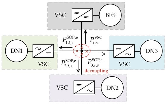
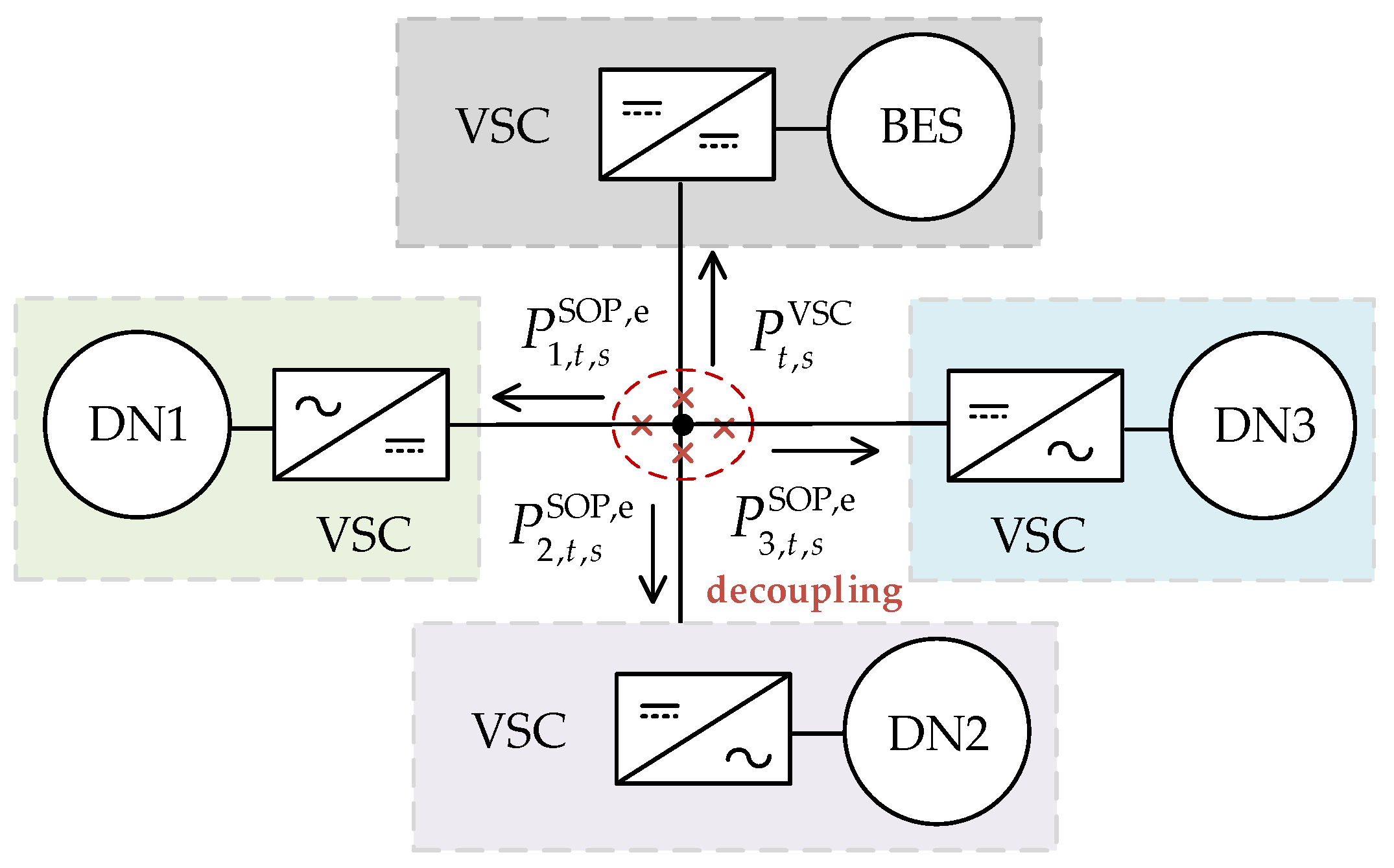
To achieve the distributed solution, the flexible interconnected distribution system is partitioned and decoupled at the common DC bus of multi-port SOP. The centralized problem is then decomposed into multiple subproblems according to subsystems, as illustrated in Figure 2.

Figure 2. Schematic diagram of E-SOP power decoupling.

The coupling relationship in Equation (31) exists among different regions. To facilitate distributed coordination, the coupling constraints are relaxed by introducing Lagrange multipliers $\lambda$, and an augmented Lagrangian function is constructed. This relaxation enables the original centralized problem to be decomposed into multiple regional subproblems, allowing the planning problem for each distribution network and shared energy storage to be represented as Equations (32) and (33), respectively.

$$\left\{\begin{array}{l}\min L_n=F_n+{\displaystyle \sum _{s\in S}{\displaystyle \sum _{t=1}^T{\lambda }_{n,s,t}\left({\displaystyle \sum _{\phi \in \left\{a,b,c\right\}}{P}_{n,s,t}^{\mathrm{SOP},\phi ,e}}+{\displaystyle \sum _{i=1,i\ne n}^N{\displaystyle \sum _{\phi \in \left\{a,b,c\right\}}{P}_{i,s,t}^{\mathrm{SOP},\phi ,e}}}+P_{s,t}^{\mathrm{VSC}}\right)}}\\ +{\displaystyle \sum _{s\in S}{\displaystyle \sum _{t=1}^T\frac{\rho }{2}{‖{\displaystyle \sum _{\phi \in \left\{a,b,c\right\}}{P}_{n,s,t}^{\mathrm{SOP},\phi ,e}}+{\displaystyle \sum _{i=1,i\ne n}^N{\displaystyle \sum _{\phi \in \left\{a,b,c\right\}}{P}_{i,s,t}^{\mathrm{SOP},\phi ,e}}}+P_{s,t}^{\mathrm{VSC}}‖}_2^2}}\\ s.t. \left(1\right),\left(3\right)-\left(4\right),\left(13\right)-\left(30\right)\end{array}\right.$$

(32)

$$\left\{\begin{array}{l}\min L=C_{inv}+C_{op}+{\displaystyle \sum _{s\in S}{\displaystyle \sum _{t=1}^T{\lambda }_{s,t}\left({\displaystyle \sum _{n=1}^N{\displaystyle \sum _{\phi \in \left\{a,b,c\right\}}{P}_{n,s,t}^{\mathrm{SOP},\phi ,e}+P_{s,t}^{\mathrm{VSC}}}}\right)}}+{\displaystyle \sum _{s\in S}{\displaystyle \sum _{t=1}^T\frac{\rho }{2}{‖{\displaystyle \sum _{n=1}^N{\displaystyle \sum _{\phi \in \left\{a,b,c\right\}}{P}_{n,s,t}^{\mathrm{SOP},\phi ,e}+P_{s,t}^{\mathrm{VSC}}}}‖}_2^2}}\\ s.t. \left(5\right)-\left(11\right),\left(13\right)-\left(14\right)\end{array}\right.$$

(33)

where ${\lambda }_{n,s,t}$ and $\rho$ denote the Lagrange multiplier and the penalty factor, respectively. By the method described above, the original problem shown in Equation (31) is decomposed into multiple local subproblems, each of which can be solved independently by the corresponding distribution network and shared energy storage unit. Each region only exchanges the optimized results of coupling variables $P_{n,s,t}^{\mathrm{SOP},\phi ,e}$ and $P_{s,t}^{\mathrm{VSC}}$, without uploading all local data. This protects the privacy of each stakeholder’s internal information while enabling coordinated distributed optimization.

3.2. Convex Reformulation of Nonconvex Constraints

The established model contains nonconvex constraints, which cannot be directly solved by existing solvers and require reformulation through convex relaxation combined with linear approximation.

3.2.1. Convex Reformulation of Rank-One Constraint

In Equation (20), the rank-one constraint represents a non-convex constraint. By relaxing the rank-one constraint and retaining only the positive semidefiniteness constraint, the remaining feasible region becomes convex, allowing the problem to be convexified and solved efficiently as a semidefinite program (SDP). After solving the relaxed SDP, if the resulting optimal matrix satisfies the rank-one condition, then this solution is also optimal for the original non-convex problem. In such cases, the semidefinite relaxation can be regarded as exact, meaning that no optimality is lost through the relaxation process [29].

3.2.2. Convex Reformulation of Capacity Constraints

The SOP capacity limit described in Equation (1) can be relaxed and reformulated as the following positive semidefinite constraint:

$$\left[\begin{array}{cc}{S}_{i,\phi ,\mathrm{SOP}}& P_{i,s,t}^{\mathrm{SOP},\phi }+j{Q}_{i,s,t}^{\mathrm{SOP},\phi }\\ P_{i,s,t}^{\mathrm{SOP},\phi }-j{Q}_{i,s,t}^{\mathrm{SOP},\phi }& S_{i,\phi ,\mathrm{SOP}}\end{array}\right]\ge 0$$

(34)

Similarly, Equation (3) and the PV capacity constraints in Equation (26) can be correspondingly relaxed into the following constraints:

$$\left[\begin{array}{cc}{S}_{i,\phi ,\mathrm{PV}}& P_{i,s,t}^{\mathrm{PV},\phi }+j{Q}_{i,s,t}^{\mathrm{PV},\phi }\\ P_{i,s,t}^{\mathrm{PV},\phi }-j{Q}_{i,s,t}^{\mathrm{PV},\phi }& S_{i,\phi ,\mathrm{PV}}\end{array}\right]\ge 0$$

(35)

$$\left[\begin{array}{cc}{P}_{i,s,t}^{\mathrm{SOP},\mathrm{loss},\phi }/A_i^{\mathrm{SOP}}& P_{i,s,t}^{\mathrm{SOP},\phi }+j{Q}_{i,s,t}^{\mathrm{SOP},\phi }\\ P_{i,s,t}^{\mathrm{SOP},\phi }-j{Q}_{i,s,t}^{\mathrm{SOP},\phi }& P_{i,s,t}^{\mathrm{SOP},\mathrm{loss},\phi }/A_i^{\mathrm{SOP}}\end{array}\right]\ge 0$$

(36)

3.2.3. Convex Reformulation of Voltage Imbalance Constraint

Equation (29) can be equivalently transformed into the following:

$$\left\{\begin{array}{l}{v}_i^a\le \left(1+\epsilon \right)v_i^{avg}\\ v_i^a\ge \left(1-\epsilon \right)v_i^{avg}\\ v_i^b\le \left(1+\epsilon \right)v_i^{avg}\\ v_i^b\ge \left(1-\epsilon \right)v_i^{avg}\\ v_i^c\le \left(1+\epsilon \right)v_i^{avg}\\ v_i^c\ge \left(1-\epsilon \right)v_i^{avg}\end{array}\right.$$

(37)

3.3. Distributed Solution Method Based on ADMM

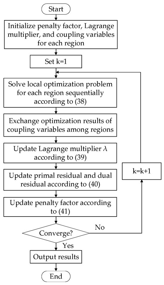
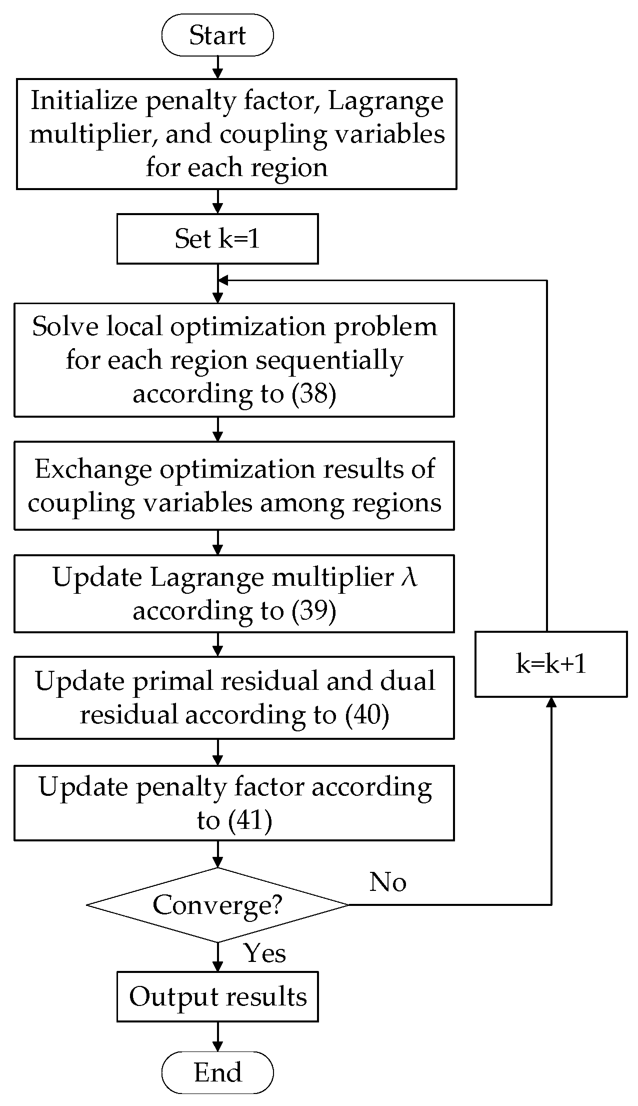
Based on the augmented Lagrangian, the ADMM decomposes the global problem into independently solvable subproblems. Taking the number of distribution networks $N=3$ as an example, the specific steps are summarized below:

Step 1: Initialize the Lagrange multiplier $\lambda$, penalty parameter $\rho$, and coupling variables for all regions. Set the iteration counter $k=1$.

Step 2: Based on the coupling power and multiplier values from the previous iteration, solve the local optimization problems sequentially:

$$\left\{\begin{array}{l}{P}_{1,s,t}^{\mathrm{SOP},\phi ,e(k+1)}=\arg \min L_1\left(P_{1,s,t}^{\mathrm{SOP},\phi ,e},P_{2,s,t}^{\mathrm{SOP},\phi ,e(k)},P_{3,s,t}^{\mathrm{SOP},\phi ,e(k)},P_{s,t}^{\mathrm{VSC}(k)},{\lambda }_{1,s,t}^{(k)}\right)\\ P_{2,s,t}^{\mathrm{SOP},\phi ,e(k+1)}=\arg \min L_2\left(P_{1,s,t}^{\mathrm{SOP},\phi ,e(k+1)},P_{2,s,t}^{\mathrm{SOP},\phi ,e},P_{3,s,t}^{\mathrm{SOP},\phi ,e(k)},P_{s,t}^{\mathrm{VSC}(k)},{\lambda }_{2,s,t}^{(k)}\right)\\ P_{3,s,t}^{\mathrm{SOP},\phi ,e(k+1)}=\arg \min L_3\left(P_{1,s,t}^{\mathrm{SOP},\phi ,e(k+1)},P_{2,s,t}^{\mathrm{SOP},\phi ,e(k+1)},P_{3,s,t}^{\mathrm{SOP},\phi ,e},P_{s,t}^{\mathrm{VSC}(k)},{\lambda }_{3,s,t}^{(k)}\right)\\ P_{s,t}^{\mathrm{VSC}(k+1)}=\arg \min L\left(P_{1,s,t}^{\mathrm{SOP},\phi ,e(k+1)},P_{2,s,t}^{\mathrm{SOP},\phi ,e(k+1)},P_{3,s,t}^{\mathrm{SOP},\phi ,e(k+1)},P_{s,t}^{\mathrm{VSC}},{\lambda }_{s,t}^{(k)}\right)\end{array}\right.$$

(38)

Step 3: Exchange the optimized results of coupling variables across regions and update the Lagrange multiplier.

$${\lambda }_{n,s,t}^{\left(k+1\right)}={\lambda }_{n,s,t}^{\left(k\right)}+\rho \left({\displaystyle \sum _{\phi \in \left\{a,b,c\right\}}\left(P_{1,s,t}^{\mathrm{SOP},\phi ,e\left(k+1\right)}+P_{2,s,t}^{\mathrm{SOP},\phi ,e\left(k+1\right)}+P_{3,s,t}^{\mathrm{SOP},\phi ,e\left(k+1\right)}\right)}+P_{s,t}^{\mathrm{VSC}\left(k+1\right)}\right)$$

(39)

Step 4: Convergence check. If the primal residual ${\delta }_1$ and dual residual ${\delta }_2$ satisfy the convergence criteria in Equation (40), terminate the iteration; otherwise, set $k=k+1$ and return to Step 2.

$$\left\{\begin{array}{l}{\delta }_1^{k+1}={‖{\displaystyle \sum _{n=1}^N{\displaystyle \sum _{\phi \in \left\{a,b,c\right\}}{P}_{n,s,t}^{\mathrm{SOP},\phi ,e(k+1)}+P_{s,t}^{\mathrm{VSC}(k+1)}}}‖}_2\le \tau \\ {\delta }_2^{k+1}=\rho {‖{\displaystyle \sum _{n=1}^N{\displaystyle \sum _{\phi \in \left\{a,b,c\right\}}\left(P_{n,s,t}^{\mathrm{SOP},\phi ,e\left(k+1\right)}-P_{n,s,t}^{\mathrm{SOP},\phi ,e\left(k\right)}\right)}}+\left(P_{s,t}^{\mathrm{VSC}(k+1)}-P_{s,t}^{\mathrm{VSC}(k)}\right)‖}_2\le \tau \end{array}\right.$$

(40)

3.4. Adaptive Penalty Factor Update Strategy

Standard ADMM’s convergence behavior and the global optimality of its solution are closely tied to the choice of the quadratic penalty factor $\rho$, whose value significantly impacts optimization outcomes [35]. When $\rho$ is fixed at an inappropriate value, standard ADMM may result in significant errors or become trapped in infeasible regions without convergence. Since it is difficult to predict a suitable $\rho$ value in advance, this paper introduces an automatic penalty factor update strategy within ADMM to ensure convergence [36]. Unlike standard ADMM with fixed $\rho$, under the proposed strategy, the quadratic penalty factor $\rho$ in the augmented Lagrangian function changes with the iteration count $k$. After each iteration, its value is updated based on the relative magnitudes of the primal residual ${\delta }_1$ and dual residual ${\delta }_2$. The update mechanism is defined as follows:

$${\rho }^{k+1}=\left\{\begin{array}{l}\alpha {\rho }^k\hspace{1em}\hspace{1em}\hspace{1em}{\delta }_1^k\ge \beta {\delta }_2^k\\ {\displaystyle \frac{{\rho }^k}{\alpha }}\hspace{1em}\hspace{1em}\hspace{1em}{\delta }_2^k\ge \beta {\delta }_1^k\\ {\rho }^k\hspace{1em}\hspace{1em}\hspace{1em}\mathrm{otherwise}\end{array}\right.$$

(41)

where $\alpha$ is a constant greater than 1, and $\beta$ denotes the residual ratio threshold between the primal and dual residuals. In this work, $\alpha =1.2$ and $\beta =10$ are used. When the primal residual ${\delta }_1^k$ is significantly larger than the dual residual ${\delta }_2^k$, the penalty factor $\rho$ is appropriately increased to place more emphasis on reducing the primal violation; conversely, when ${\delta }_1^k$ is relatively smaller than ${\delta }_2^k$, $\rho$ is decreased to give relatively more weight to the dual conditions. This adaptive strategy helps avoid convergence failure associated with an unsuitable initial choice of penalty parameter.

Algorithm steps for solving the unbalanced flexible interconnected distribution networks coordinated planning model using the above accelerated ADMM method are shown in Figure 3.

Figure 3. Model solution flowchart.

3.5. Cost Allocation Based on the Shapley Value

When distribution networks belong to different stakeholders, a fair cost-sharing mechanism must be established to allocate the total cost among the different networks when multiple distribution networks jointly invest in PV and E-SOP. The Shapley value method is a solution concept from cooperative game theory that allocates the cooperative gains or costs based on the marginal contribution of each participant to the coalitions they join [37]. This approach effectively resolves conflicts that arise from benefit or cost allocation among multiple agents during cooperation, and it ensures both rationality and fairness of the allocation.

The core principle of the Shapley value method is that the cost borne by a participant is determined by the incremental cost generated when joining the coalition. Since the marginal contribution varies depending on the joining sequence, the Shapley value considers all possible permutations of participant entry and computes a weighted average. Based on this method, assume the set of distribution networks participating in the cooperative game is $N$, with $n$ representing the total number of networks. When $n$ networks form a cooperative coalition in random sequences, the probability $p$ of each sequence occurring is as follows:

$$p={\displaystyle \frac{1}{n!}}$$

(42)

Considering the scenario where distribution network $i$ joins to form a sub-coalition $m$ of size $\left|m\right|$, before network $i$ joins, there are already $\left|m\right|-1$ participants in the coalition, and after its inclusion, there remain $n-\left|m\right|$ participants. In this situation, there are $(|m|-1)!(n-|m|)!$ different ordering permutations of the coalition. Let $\varphi \left(m_i\right)$ represent the probability of such a coalition sequence occurring. Then $\varphi \left(m_i\right)$ can be calculated as follows:

$$\varphi \left(m_i\right)=p(|m|-1)!(n-|m|)!={\displaystyle \frac{(|m|-1)!(n-|m|)!}{n!}}$$

(43)

Based on Equation (43), the cost apportioned to distribution network $i$ can be calculated as follows [38]:

$$C_i\left(v\right)={\displaystyle \sum }_{m\subseteq N,i\in m}{\displaystyle \frac{(|m|-1)!(n-|m|)!}{n!}}[v(m)-v(m\backslash \{i\})]$$

(44)

where $v(m)$ represents the total cost of coalition $m$ when the distribution network $i$ participates in it, and $v(m\backslash \{i\})$ denotes the cost of coalition $m$ without network $i$. The term $[v(m)-v(m\backslash \left\{i\right\})]$ represents the incremental cost contributed by the distribution network $i$ upon joining the coalition. When applying the Shapley value method for cost allocation, the cost allocated to each distribution network depends on the marginal cost it contributes to the coalition as a result of joining, i.e., the amount by which the coalition’s cost increases due to that network’s participation. This reflects the Shapley value’s core principle of allocating based on marginal contributions.

4. Case Study

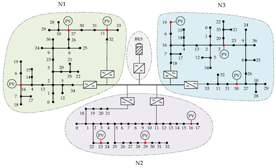
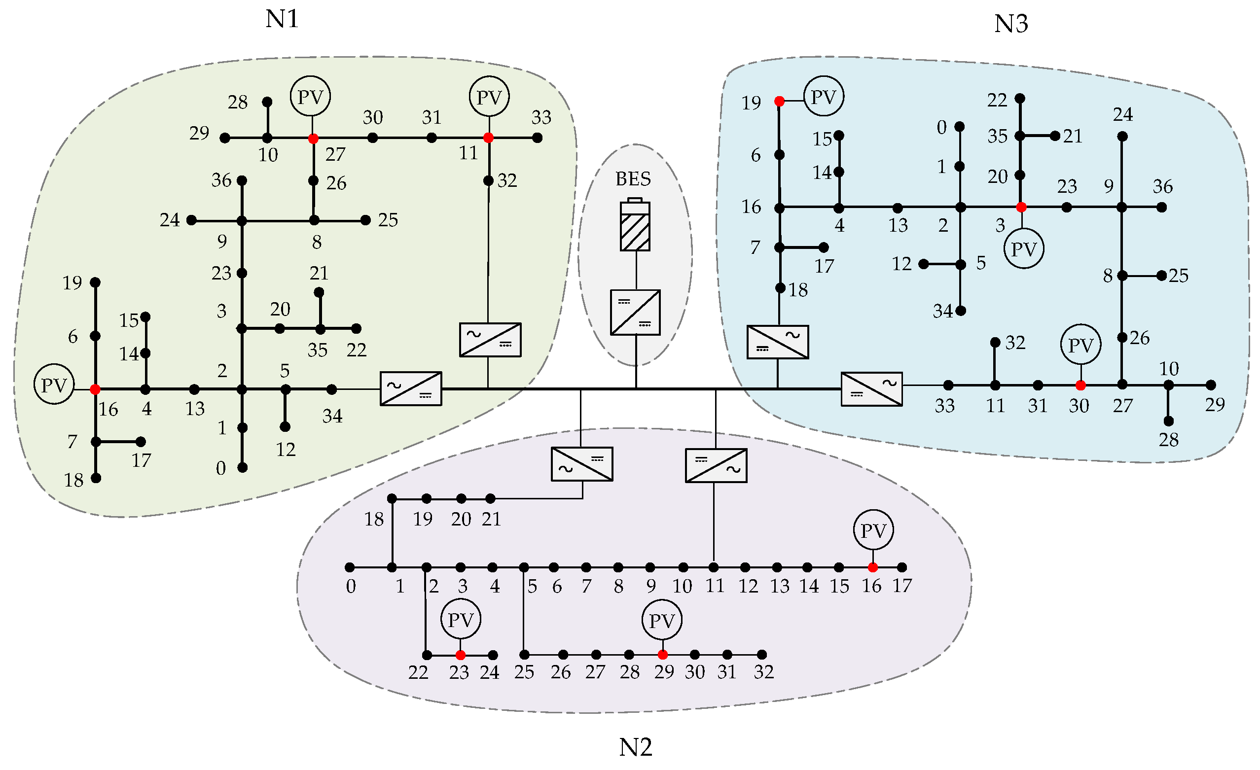
In this section, the effectiveness of the proposed method is validated using the flexible interconnected distribution system shown in Figure 4. The system is composed of three distribution networks, N1, N2, and N3, which are flexibly interconnected through E-SOP. N1 and N3 are constructed based on the modified IEEE 37 bus distribution feeder [39], while N2 is developed from the modified IEEE 33 node distribution feeder [40]. The IEEE 33 bus and IEEE 37 bus feeders are widely used benchmark systems in distribution network studies and can represent the typical characteristics of practical distribution networks. During the planning phase, the connection locations of the multi-terminal SOP can be determined based on the actual conditions of the distribution system. For the convenience of research, this paper selects nodes at traditional tie switches, as well as several nodes with high load proportions and frequent voltage violations, as the access points for the E-SOP. In addition, nodes 11, 16, and 27 in distribution network N1, nodes 16, 23, and 29 in network N2, and nodes 3, 19, and 30 in network N3 are set as candidate PV access nodes for their respective networks.

Figure 4. Topology of flexible interconnected distribution system.

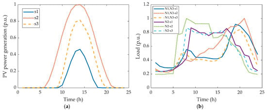
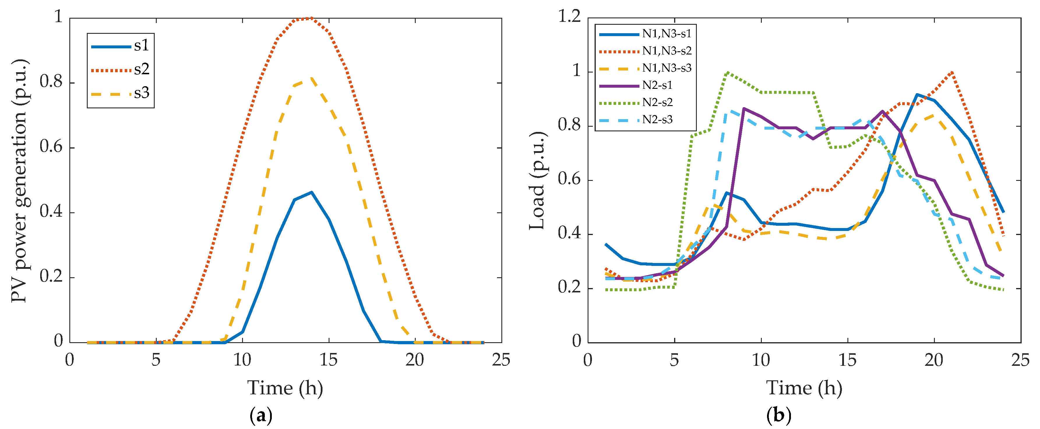
In this study, three representative scenarios are considered to capture different operating conditions. This scenario-based approach is used to balance modeling accuracy and computational efficiency. Figure 5 shows the PV output and load curves under three typical scenarios (i.e., s1, s2, and s3). The scenario probabilities are defined as 0.25 for s1 and s2, and 0.50 for s3. The PV generation profiles and load scenarios are derived from the Open Energy Information platform [41]. The PV output curves of the three distribution networks are identical, and the load curves of distribution networks N1 and N3 are the same. Other case parameters are listed in Table 2, while the admissible ranges of the optimization variables are specified in Table 3. These parameters used in this study are set based on typical values in the related literature [42,43].

Figure 5. Photovoltaic and load curves of distribution networks. (a) PV output; (b) load curves.

Table 2. System parameters.

Parameter	Value	Parameter	Value	Parameter	Value
$d$	0.08	$c_{\mathrm{DCDC}}$ *	0.5	${\eta }_d$	0.9
$y$	20	$c_{op}^{\mathrm{PV}}$ *	0.0001	$S_{\min }^{\mathrm{SOC}}$	0.1
$c_{\mathrm{PV}}$ *	5	$A_i^{\mathrm{SOP}}$	0.02	$S_{\max }^{\mathrm{SOC}}$	0.9
$c_{\mathrm{SOP}}$ *	1.5	$\cos {\theta }_{\min }^{\mathrm{PV}}$	0.9	$\gamma$	0.01
$c_{\mathrm{BES}}$ *	2	${\eta }_c$	0.9	$\tau$	0.01

* Unit: $c_{\mathrm{PV}}$ is in 10³ CNY/kW; $c_{\mathrm{BES}}$ and $c_{op}^{\mathrm{PV}}$ are in 10³ CNY/kWh $c_{\mathrm{SOP}}$ and $c_{\mathrm{DCDC}}$ are in 10³ CNY/kVA.

Table 3. Variable range.

Variable	Minimum	Maximum	Variable	Minimum	Maximum
$S_{i,3\phi ,\mathrm{PV}}$	0	2 MW	$u_{s,t}^{ch}$	0	1
$S_{i,3\phi ,\mathrm{SOP}}$	0	1.5 MVA	$u_{s,t}^{dis}$	0	1
$Q_{i,s,t}^{\mathrm{SOP},\phi }$	−500 kvar	500 kvar	$v_{i,s,t}$	0.9025 p.u.	1.1025 p.u.

4.1. Benefit Analysis of E-SOP

4.1.1. Economic Analysis

To evaluate the effectiveness of coordinated E-SOP configuration among different distribution networks, four schemes are employed for simulation and comparative analysis:

• Case I: The original three-phase unbalanced network.
• Case II: Coordinated configuration of PV and multi-terminal SOP in distribution networks without battery energy storage integration.
• Case III: Individual planning of PV and E-SOP in each distribution network, which means integrating energy storage systems into the two-terminal SOP of each network, and the networks are not interconnected.
• Case IV: Coordinated configuration of PV and multi-terminal E-SOP in distribution networks.

The optimization results for the different schemes are presented in Table 4, Table 5, Table 6 and Table 7:

Table 4. Cost optimization results of different cases.

Cost (103 CNY)	Case I	Case II	vs. Case I	Case III	vs. Case I	Case IV	vs. Case I
Total Cost	46,950.4	40,216.3	−14.34%	40,216.0	−14.34%	39,952.7	−14.90%
Investment Cost	-	3646.3	-	5038.4	-	4997.6	-
O&M Cost	-	1303.1	-	1439.8	-	1435.7	-
Electricity Purchase Cost	46,950.4	35,266.9	−24.88%	33,737.8	−28.14%	33,519.4	−28.61%

Table 5. PV configuration results in each case.

Network	Case I Node (MW)	Case II Node (MW)	Case III Node (MW)	Case IV Node (MW)
N1	-	11 (0.34)	11 (0.34)	11 (0.25)
		16 (0.34)	16 (0.35)	16 (0.38)
		27 (0.62)	27 (0.61)	27 (0.66)
N2	-	16 (0.62)	16 (0.60)	16 (0.59)
		23 (0.06)	23 (0.19)	23 (0.14)
		29 (1.51)	29 (1.39)	29 (1.45)
N3	-	3 (1.12)	3 (1.27)	3 (1.23)
		19 (0.58)	19 (0.60)	19 (0.58)
		30 (1.54)	30 (1.37)	30 (1.43)

Table 6. SOP configuration results in each case.

Network	Case I Node (MVA)	Case II Node (MVA)	Case III Node (MVA)	Case IV Node (MVA)
N1	-	32 (0.19)	32 (0.73)	32 (0.51)
		34 (0)	34 (0.26)	34 (0.30)
N2	-	11 (0.29)	11 (0.75)	11 (0.56)
		21 (0)	21 (0.14)	21 (0.11)
N3	-	18 (0.21)	18 (0.28)	18 (0.28)
		33 (0.78)	33 (0.80)	33 (0.80)

Table 7. Energy storage and DC/DC converter configuration results in each case.

Network	Case I (MWh/MVA)	Case II (MWh/MVA)	Case III (MWh/MVA)	Case IV (MWh/MVA)
N1	-	-	2.18/0.97	5.61/2.49
N2	-	-	1.96/0.87
N3	-	-	1.37/0.61

In Case I, the total cost is determined solely by the amount paid for power supplied by the upstream network. Compared with Case I, Cases II–IV significantly reduce the total system cost by introducing PV generation and SOP. In Cases II–IV, the total installed PV capacity across all distribution networks reaches the predefined maximum PV penetration level, though installation capacities vary slightly across nodes. Compared with Case II, Case III enables more flexible control of active power transmission between nodes through integrated energy storage. This allows energy to be exchanged not only among networks but also optimized across time periods via storage-based dispatching, thereby enhancing power flow optimization capability and substantially reducing electricity purchase costs. However, due to increased investment in SOP port capacity and battery energy storage construction, the overall investment and O&M costs of equipment increase substantially. Consequently, the total cost only slightly decreases compared to Case II.

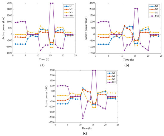
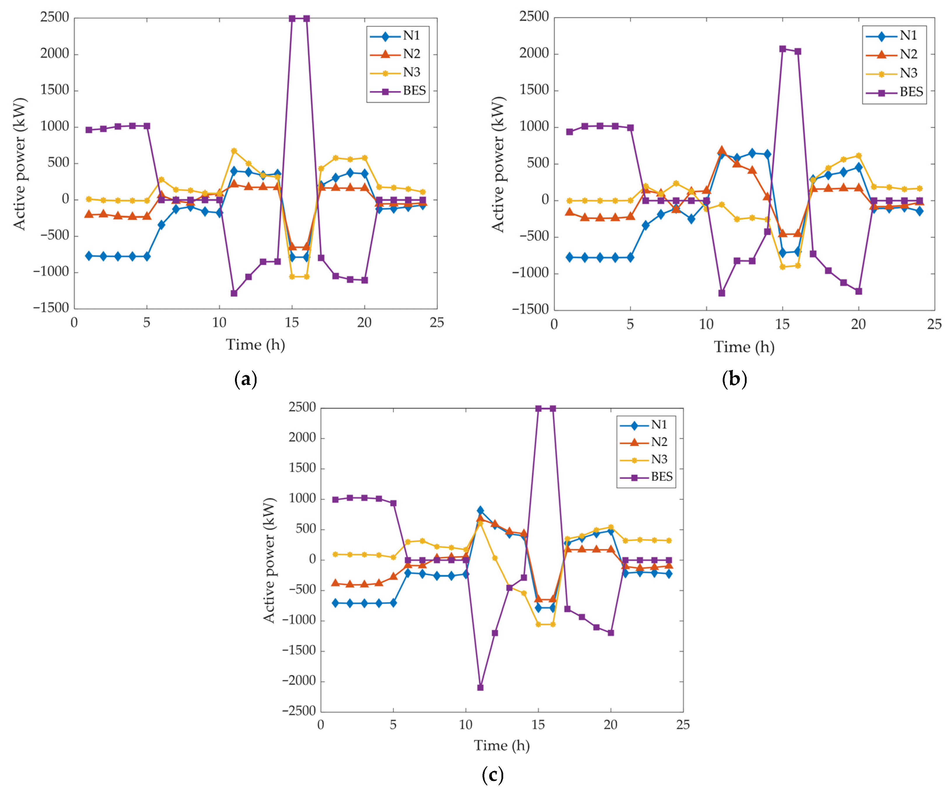
Compared to Case III, Case IV achieves cross-regional resource sharing through collaborative planning and utilization of E-SOP across different distribution networks. In Case IV, the shared BES is connected to the common DC bus of the multi-terminal SOP, allowing energy to be dispatched across all three networks. Unlike dedicated storage that serves only a single network, the shared configuration enables temporal and spatial flexibility: excess PV generation from one network can be stored and later released to another network during peak load hours. The shared E-SOP can enhance operational flexibility, improve the utilization of both SOP and storage resources, and avoid redundant investments, thus resulting in reduced total investment and O&M costs. As shown in Table 4, Case IV exhibits the best economic performance, with the electricity purchase cost decreased by 13.431 million CNY (28.61%) and the total annual comprehensive system cost reduced by 6.998 million CNY (14.90%) compared to the pre-planning stage. Figure 6 shows the active power output of the E-SOP to each distribution network under different scenarios, as well as the charge and discharge power of the shared energy storage.

Figure 6. Active power output of E-SOP to each region under different scenarios. (a) scenario 1; (b) scenario 2; (c) scenario 3.

As shown in Figure 6, in Case IV, multi-terminal SOP enables active power exchange both within feeder lines of the same network and between different subnetworks. There is no longer only a single power flow path between nodes within a network, and active power support can be provided between different networks. The integration of energy storage further contributes positively to peak shaving and valley filling, reducing the system’s peak power purchases and minimizing electrical energy losses. Compared to individual planning of PV and E-SOP within separate distribution networks, collaborative planning and utilization of PV and E-SOP fully leverage distributed energy resources. This approach reduces overall system planning and operational costs and improves the economic performance of the flexible interconnected distribution system.

4.1.2. Voltage Quality Analysis

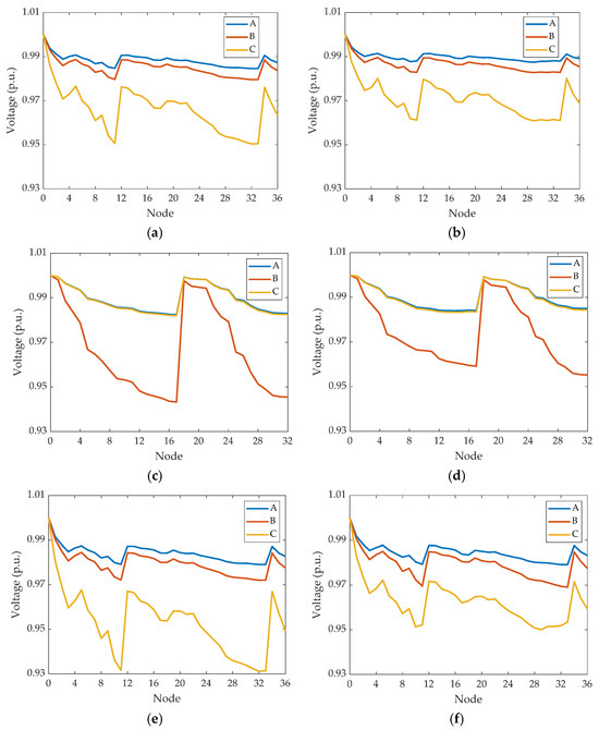
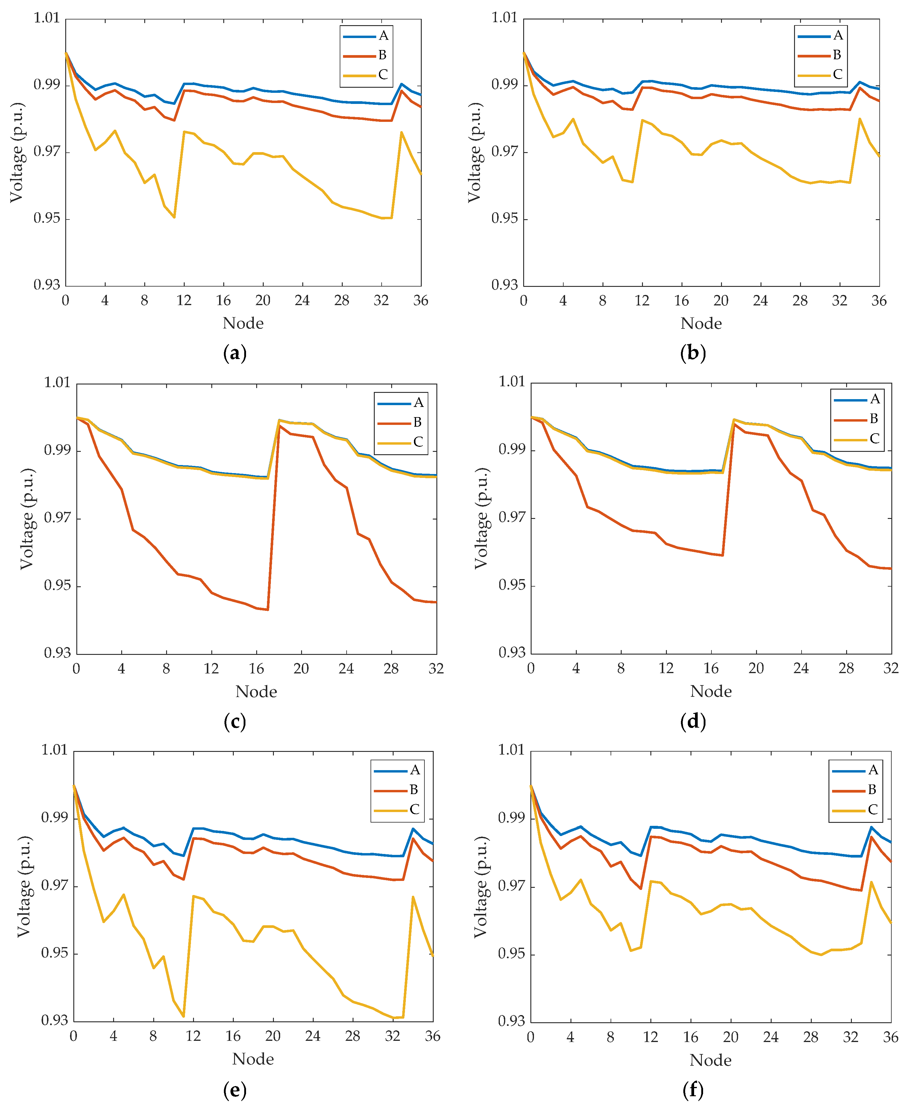
Table 8 presents the maximum voltage imbalance of each distribution network in Cases I–IV. Figure 7 depicts the three-phase voltage curves at the moment of maximum voltage imbalance for each distribution network without PV and E-SOP, as well as the corresponding three-phase voltage curves under Case IV at the same time instant.

Table 8. The maximum voltage imbalance of each distribution network in different cases.

Network	Case I	Case II	Case III	Case IV
N1	2.18%	2%	2%	2%
N2	2.68%	2%	2%	2%
N3	3.08%	2%	2%	2%

Figure 7. Three-phase voltage profile of each distribution network at the same moment in Case I and IV. (a) N1 in Case I; (b) N1 in Case IV; (c) N2 in Case I; (d) N2 in Case IV; (e) N3 in Case I; (f) N3 in Case IV.

As shown in Table 8 and Figure 7, in the initial state, the three-phase voltages of each distribution network differ significantly, and the voltage imbalance for all networks exceeds the threshold of 2% [32]. Furthermore, without PV and E-SOP integration, the voltages in distribution networks 2 and 3 fall below the safety voltage lower limit. Case IV demonstrates substantial voltage quality improvement through optimized PV and E-SOP configuration. The voltage magnitudes of N1, N2, and N3 increased, and the maximum voltage unbalance reduced from 2.18%, 2.68%, and 3.08% in Case I to 2.00% in Case IV for N1, N2, and N3, respectively. This corresponds to reductions of 0.18, 0.68, and 1.08 percentage points, or 8.26%, 25.37%, and 35.06% in relative terms. Table 8 and Figure 7 demonstrate that the proposed coordinated planning effectively improves the overall voltage profile by simultaneously reducing phase unbalance and increasing voltage magnitudes.

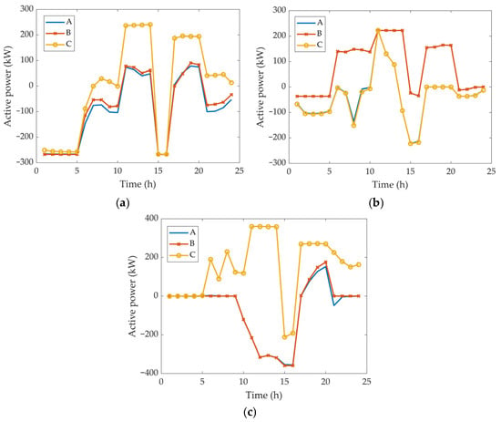
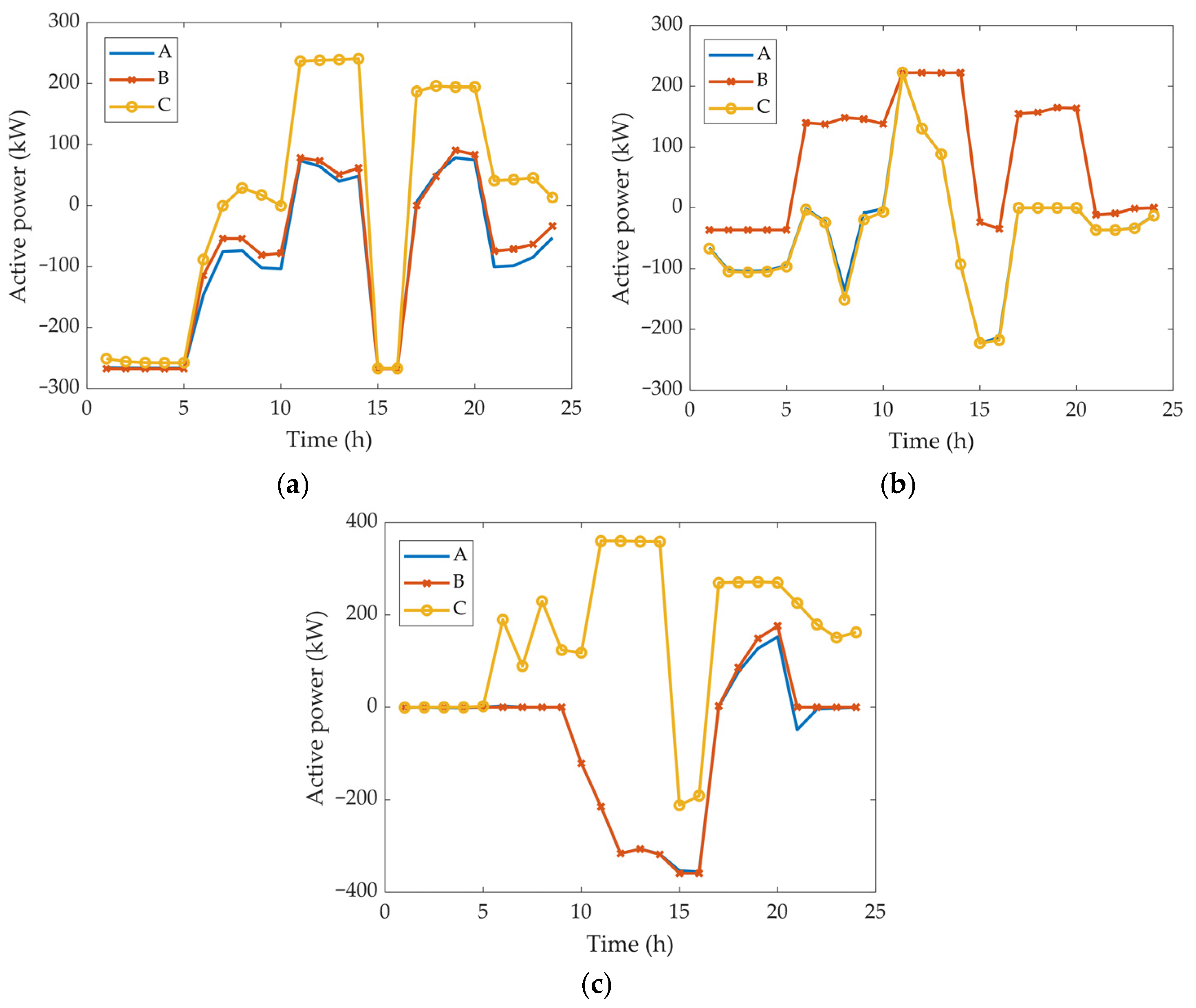
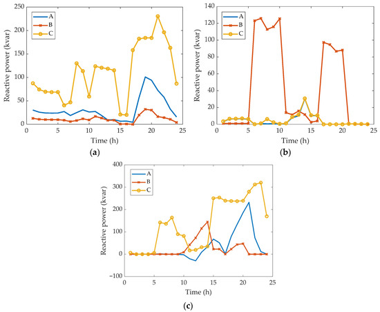
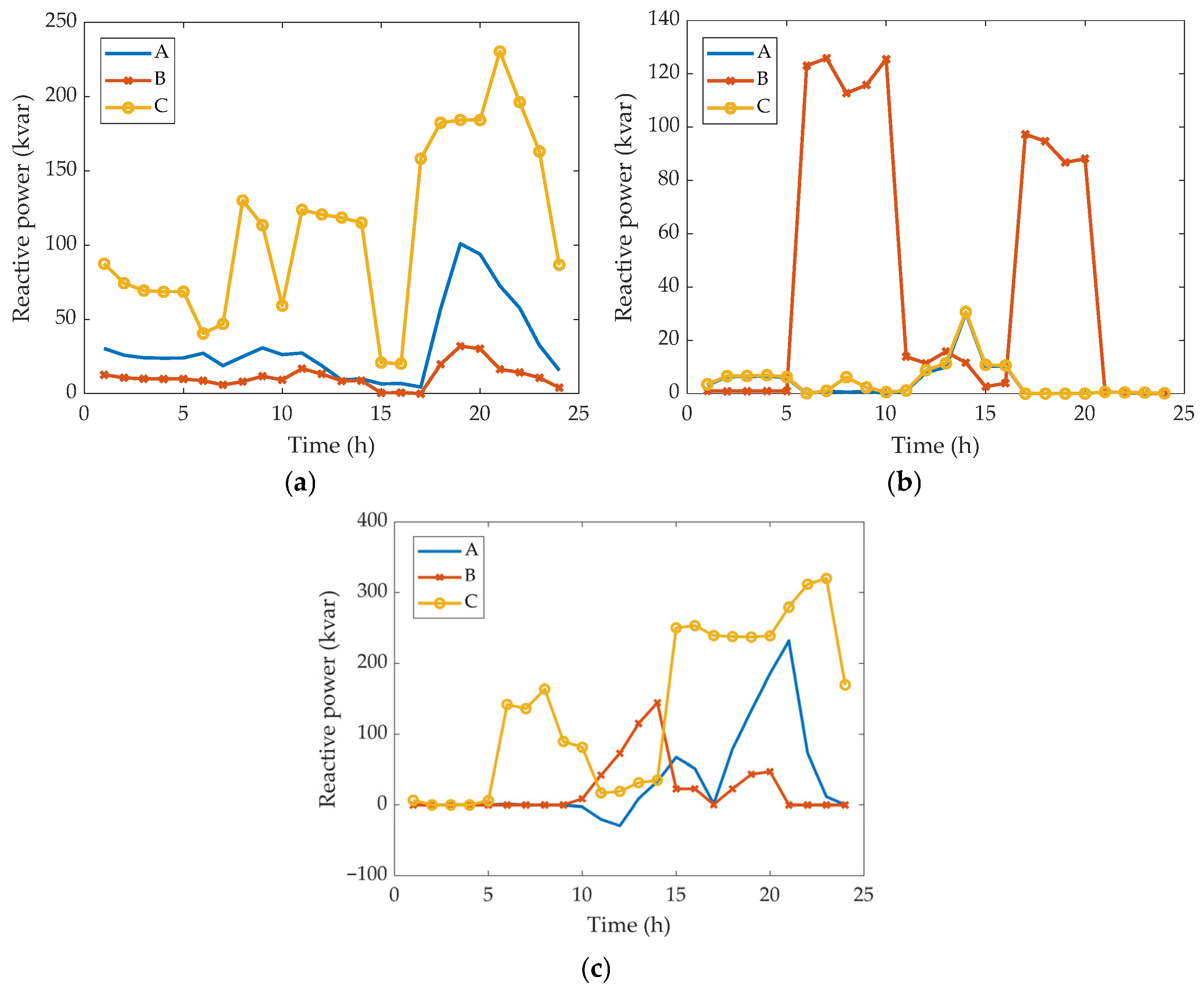
Figure 8 shows the 24 h active power outputs of the SOP in each distribution network under the corresponding scenarios, and Figure 9 shows the 24 h reactive power outputs of the SOP in each network for Case IV. By leveraging the flexible phase-wise power control capability of E-SOP, not only can active power be transferred and optimally allocated between different phases within the same feeder, but three-phase power support can also be realized across subnetworks, further enhancing the system’s power flow control capability. Furthermore, the converters connected in each distribution network can provide phase-specific reactive power compensation within their capacity limits. Ultimately, Case IV significantly reduces voltage imbalance and improves voltage waveforms.

Figure 8. Three-phase active power output of SOP in each network. (a) Active power output of SOP in N1; (b) active power output of SOP in N2; (c) active power output of SOP in N3.

Figure 9. Three-phase reactive power output of SOP in each network. (a) Reactive power output of SOP in N1; (b) reactive power output of SOP in N2; (c) reactive power output of SOP in N3.

4.2. Cost Allocation

Coordinated planning of PV and E-SOP across multiple distribution networks can effectively reduce the system’s comprehensive operational cost. However, as this involves more than one participant, the issue of apportioning the total cost among stakeholders arises. To address this cost-sharing problem, the Shapley value method proposed in Section 3 is applied in the following analysis. In this study, the participants considered are the three distribution networks, and there are five possible strategy patterns as shown in Table 9, where each game mode corresponds to a different degree of cooperation among the distribution networks.

Table 9. Possible strategy patterns.

Game Mode	Description	Degree of Cooperation
{N1} {N2} {N3}	N1, N2, and N3 plan completely independently.	Non-cooperative
{N1 N2} {N3}	N1 and N2 form a coalition for coordinated planning; N3 plans independently.	Partial cooperation
{N1 N3} {N2}	N1 and N3 form a coalition for coordinated planning; N2 plans independently.	Partial cooperation
{N2 N3} {N1}	N2 and N3 form a coalition for coordinated planning; N1 plans independently.	Partial cooperation
{N1 N2 N3}	N1, N2, and N3 plan collaboratively.	Full cooperation

The cost of each coalition under different game modes, as well as the cost allocation results for each distribution network using the Shapley value method, are presented in Table 10 and Table 11, respectively.

Table 10. Cost of each coalition under different game modes.

Coalition	Cost (103 CNY)
{N1}	12,429.1
{N2}	13,505.4
{N3}	14,281.6
{N1 N2}	25,933.1
{N1 N3}	26,537.7
{N2 N3}	27,606.3
{N1 N2 N3}	39,952.7

Table 11. Cost allocation results for each distribution network.

Game Mode	N1 (103 CNY)	N2 (103 CNY)	N3 (103 CNY)	Total Cost (103 CNY)
{N1} {N2} {N3}	12,429.1	13,505.4	14,281.6	40,216.1
{N1 N2} {N3}	12,428.4	13,504.7	14,281.6	40,214.7
{N1 N3} {N2}	12,342.6	13,505.4	14,195.1	40,043.1
{N2 N3} {N1}	12,429.1	13,415.1	14,191.2	40,035.4
{N1 N2 N3}	12,372.5	13,444.9	14,135.3	39,952.7

It is evident from Table 11 that as the degree of cooperation increases, the overall system cost gradually decreases. Under the mode where each distribution network independently configures PV and E-SOP, the system exhibits the highest overall annual cost. In contrast, participating in co-construction and sharing of flexibility resources reduces the operational costs for each distribution network. The total cost of the fully cooperative coalition {N1 N2 N3} is significantly lower than the total cost under the non-cooperative condition and also lower than that under partial cooperation. This indicates that by engaging in coordinated planning, the three distribution networks fully leverage economies of scale and complementarities, thereby achieving minimization of the total cost. These cost savings arise from resource sharing and power exchange, avoiding redundant investment and inefficient operation, which reflects collective rationality of cooperative games.

The stability of a coalition depends on the individual rationality of each distribution network. It is necessary to determine whether any sub-coalition or single member has an incentive to deviate, that is, whether any sub-coalition or single participant can achieve a lower individual cost by abandoning the fully cooperative arrangement. When using the Shapley value for cost allocation, in the fully cooperative coalition {N1 N2 N3}, the allocated cost for each distribution network is lower than its cost under non-cooperative circumstances. Therefore, each distribution network has an incentive to participate in the fully cooperative coalition, satisfying individual rationality. Although certain sub-coalitions might benefit specific networks—for instance, Network 1 incurs lower costs in sub-coalition {N1 N3}, and Network 2 in {N2 N3}—Network 3’s allocated costs in these sub-coalitions exceed those in the full cooperation coalition. Consequently, Network 3 lacks motivation to join sub-coalitions and prefers full cooperation, making these sub-coalitions unstable. No sub-coalition is able to improve the costs of all its members simultaneously, indicating that the fully cooperative coalition lies within the core of the cooperative game.

In summary, the coalition {N1 N2 N3} is the cost-optimal coalition structure. Moreover, the allocation strategy based on the Shapley value ensures fairness and rationality in cost apportionment among distribution networks, thereby enhancing the enthusiasm of each region to participate in joint construction. This fully demonstrates the economic value and cooperative stability of multi-distribution network coordinated planning.

4.3. Algorithm Convergence Analysis

4.3.1. Convergence Performance Under Different Initial Penalty Factors

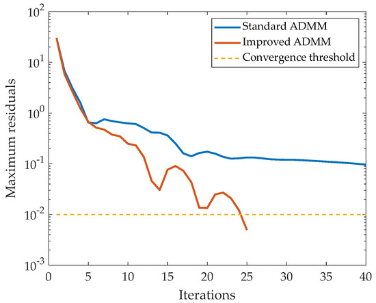
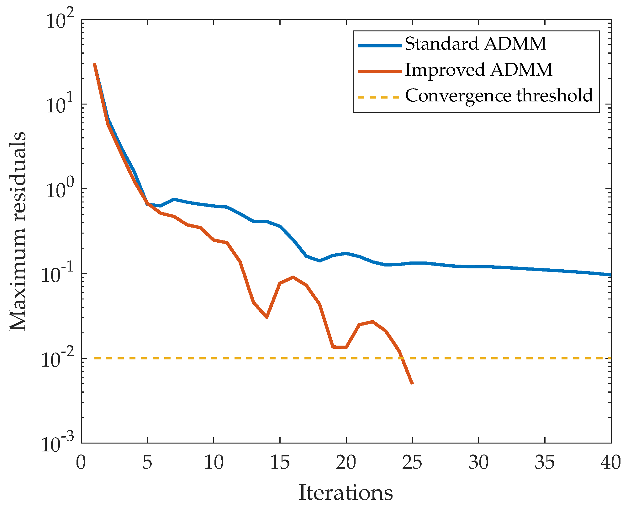
This paper introduces an adaptive penalty factor update strategy to improve the ADMM algorithm. To evaluate the proposed distributed solution strategy, three representative methods are compared in this study. The centralized method is used as the benchmark for solution quality and optimality reference, the standard ADMM is selected as a widely used baseline distributed algorithm, and the improved ADMM is adopted to verify the effectiveness of the proposed adaptive penalty update strategy. This comparison focuses on convergence behavior, computational efficiency, and solution accuracy under the same planning model. The annual comprehensive costs obtained by the three methods are presented in Table 12. The residual iteration processes during the solution of the distributed planning model using the standard ADMM algorithm and the improved ADMM algorithm are illustrated in Figure 10. The residual in the figure represents the maximum value between the primal and dual residuals during the iterative process.

Table 12. Solution results of different algorithms.

Algorithm	Cost (103 CNY)	Number of Iterations	Relative Gap vs. Centralized
Centralized Method	39,944.9	-	0
Standard ADMM	-	40 times	-
Improved ADMM	39,952.7	25 times	0.02%

Figure 10. Comparison of residual iteration trends between standard and improved ADMM.

Table 12 and Figure 10 demonstrate that with an initial penalty factor $\rho =0.02$, the standard ADMM algorithm fails to converge even after 40 iterations. In contrast, the improved ADMM algorithm achieves convergence to a value close to the centralized optimization result within 25 iterations. The experimental results prove that inappropriate penalty parameters can prevent standard ADMM from converging. By introducing an automatic penalty factor update strategy, the penalty parameter can be adjusted to a suitable magnitude during iterations, which both ensures the convergence of ADMM and accelerates its convergence speed. The proposed improved ADMM algorithm therefore exhibits good applicability in distributed planning problems.

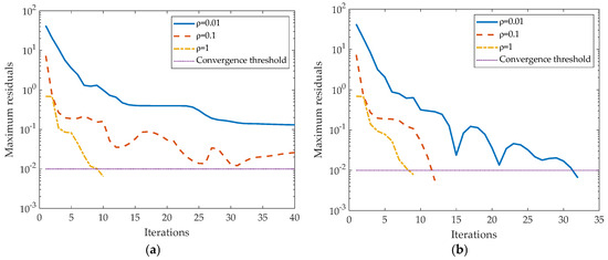
To further investigate the effect of the penalty factor $\rho$ on algorithmic convergence performance, this case study examines the iteration performance of the standard ADMM and the improved ADMM under different initial penalty factors. The model is solved using both methods with varying initial $\rho$ values. The results are presented in Table 13, and the residual iteration processes are illustrated in Figure 11.

Table 13. Solution results under different initial penalty parameters.

Initial Penalty Parameter	Algorithm	Cost (103 CNY)	Number of Iterations	Relative Gap vs. Centralized
0.01	Standard ADMM	-	40 times	-
	Improved ADMM	39,962.3	32 times	0.04%
0.1	Standard ADMM	-	40 times	-
	Improved ADMM	40,023.0	12 times	0.20%
1	Standard ADMM	40,175.6	10 times	0.58%
	Improved ADMM	40,173.8	9 times	0.57%

Figure 11. Comparison of residual iteration trends under different initial penalty parameters. (a) Standard ADMM; (b) improved ADMM.

Table 13 and Figure 11 reveal that the convergence of standard ADMM cannot be guaranteed when the penalty factor is inappropriately set. Specifically, with $\rho =0.01$ and $\rho =0.1$, the standard ADMM still does not converge to within the allowable residual threshold after 40 iterations. When $\rho$ increases to 1, the number of iterations decreases significantly, but the objective value deviates from the centralized optimal solution. These simulation results confirm that the performance of the standard ADMM is highly sensitive to the selection of the penalty parameter. When $\rho$ is too small, the local subproblems tend to focus primarily on minimizing their own local cost, partially neglecting the coupling constraints with neighboring regions, which leads to slow overall convergence. Conversely, when $\rho$ is overly large, the augmented penalty term may become overly dominant, making it difficult for the algorithm to balance between feasibility and optimality, thus negatively affecting the quality of the final solution.

Compared with the standard ADMM, the improved ADMM exhibits clear advantages under the same initial $\rho$ settings. For $\rho =0.01$ and $\rho =0.1$, the improved ADMM converges within 32 and 12 iterations, respectively, which is significantly faster than the traditional ADMM. When $\rho =1$, the improved ADMM also requires fewer iterations and produces results that are closer to the centralized optimal value. These results validate that the convergence of ADMM is sensitive to the penalty factor selection and prove that the residual ratio-based dynamic penalty parameter updating strategy effectively enhances convergence efficiency and solution quality.

4.3.2. Influence of Adaptive Update Strategy Parameters on Optimality

To further justify the selection of hyperparameters in the adaptive penalty factor update strategy, a sensitivity analysis was conducted regarding the growth coefficient $\alpha$ and the residual ratio threshold $\beta$. The impact of changes in these parameters on the total planning cost and the number of iterations is summarized and discussed. The results are shown in Table 14 and Table 15.

Table 14. Solution results with different initial penalty parameters and growth coefficients.

Initial Penalty Parameter	$\mathit{\alpha }$	$\mathit{\beta }$	Cost (103 CNY)	Number of Iterations	Relative Gap vs. Centralized
0.01	1.2	10	39,962.3	32 times	0.04%
	2.4	10	40,690.6	11 times	1.87%
	3.6	10	40,561.7	11 times	1.54%
0.1	1.2	10	40,023.0	12 times	0.20%
	2.4	10	40,067.5	11 times	0.31%
	3.6	10	40,061.1	11 times	0.29%
1	1.2	10	40,173.8	9 times	0.57%
	2.4	10	40,155.9	8 times	0.53%
	3.6	10	40,128.3	9 times	0.46%

Table 15. Solution results with different initial penalty parameters and residual ratio thresholds.

Initial Penalty Parameter	$\mathit{\alpha }$	$\mathit{\beta }$	Cost (103 CNY)	Number of Iterations	Relative Gap vs. Centralized
0.01	1.2	5	39,972.9	21 times	0.07%
	1.2	10	39,962.3	32 times	0.04%
	1.2	15	39,960.1	32 times	0.04%
0.1	1.2	5	40,054.7	12 times	0.27%
	1.2	10	40,023.0	12 times	0.20%
	1.2	15	40,023.0	12 times	0.20%
1	1.2	5	40,173.8	9 times	0.57%
	1.2	10	40,173.8	9 times	0.57%
	1.2	15	40,173.8	9 times	0.57%

Based on the results in Table 14, the following conclusions can be drawn. When $\rho =0.01$ and $\rho =0.1$, although increasing $\alpha$ from 1.2 to 2.4 or 3.6 can reduce the number of iterations, this leads to an increase in the total planning cost. For example, the cost rises from 39,962.3 to 40,690.6 when $\rho =0.01$. This suggests that an aggressive increase in the penalty factor may cause the algorithm to converge prematurely to a sub-optimal solution. In comparison, when $\rho =1$, the excessively large initial penalty factor imposes an extremely high penalty on constraint violations during the early iterations, forcing the algorithm into a sub-optimal feasible region. In this case, the adjustment of the $\alpha$ value has a limited impact. The relative gaps between the distributed results and the centralized solution remain above 0.4% across different $\alpha$ values.

The results in Table 15 show that the proposed algorithm is not highly sensitive to $\beta$. When $\alpha$ is fixed at 1.2, varying $\beta$ from 5 to 15 leads to only minor changes in the final annual cost, while the number of iterations remains within a similar range under most initial penalty settings. This indicates that $\beta$ mainly affects the triggering frequency of the update rule but has a limited impact on the final optimization result. Therefore, following the common practice in the distributed optimization literature [44], $\beta =10$ is adopted as a balanced threshold and is advisable to maintain a stable ratio between primal and dual residuals.

In summary, selecting a relatively smaller initial penalty factor to preserve flexibility in the search space, while setting a relatively mild growth strategy, enables the improved ADMM algorithm to accelerate convergence compared to the standard ADMM while ensuring optimality.

4.4. Verification of SDP Relaxation Accuracy

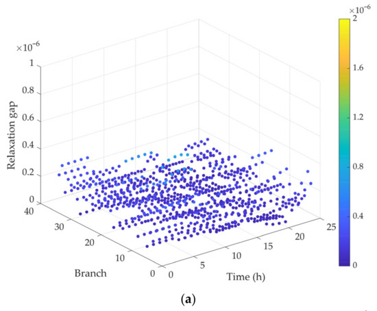
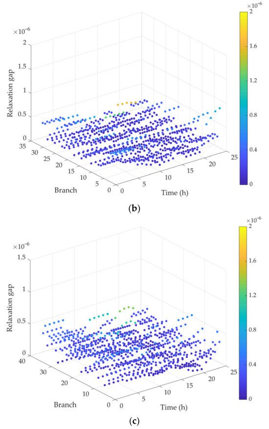
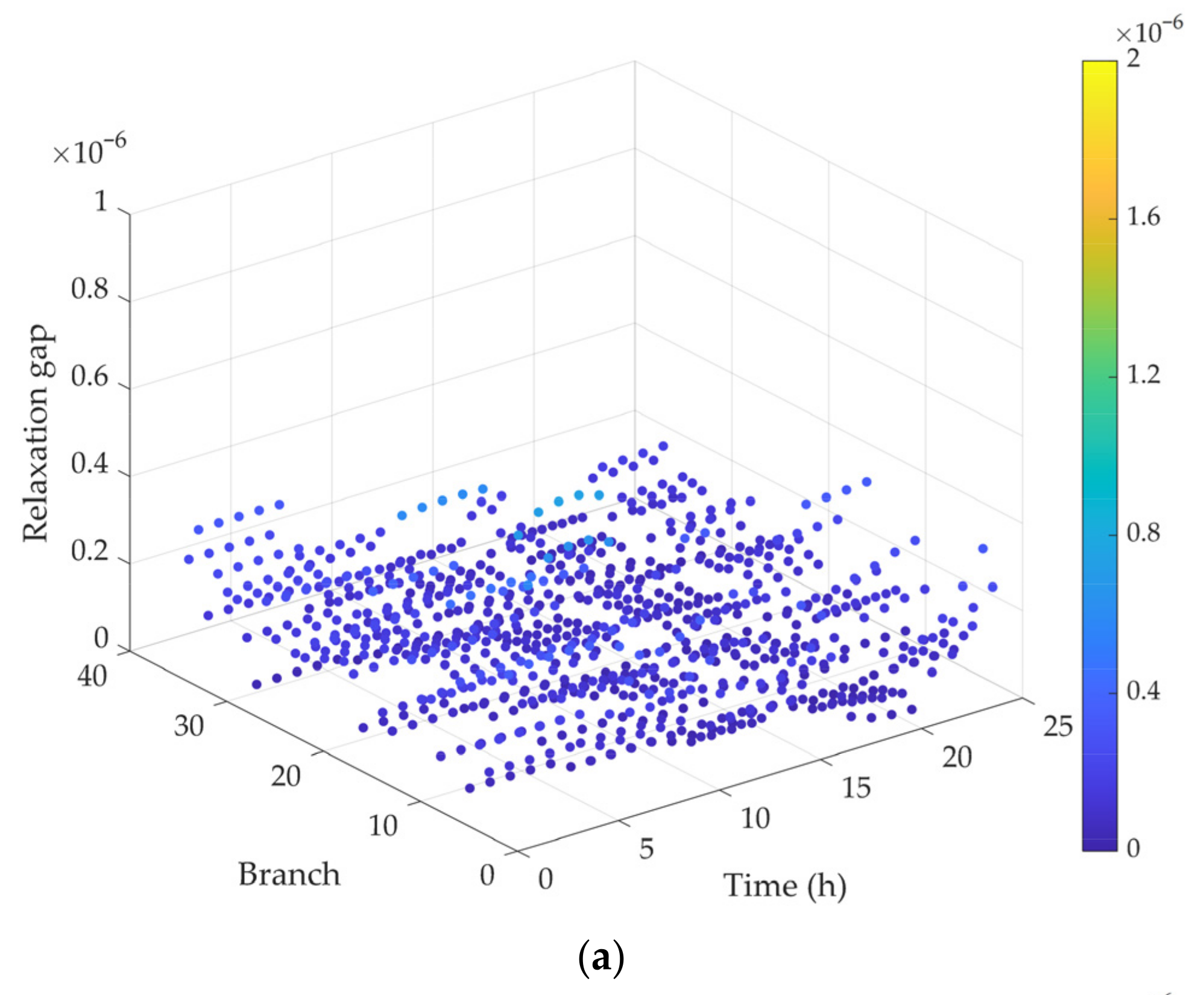
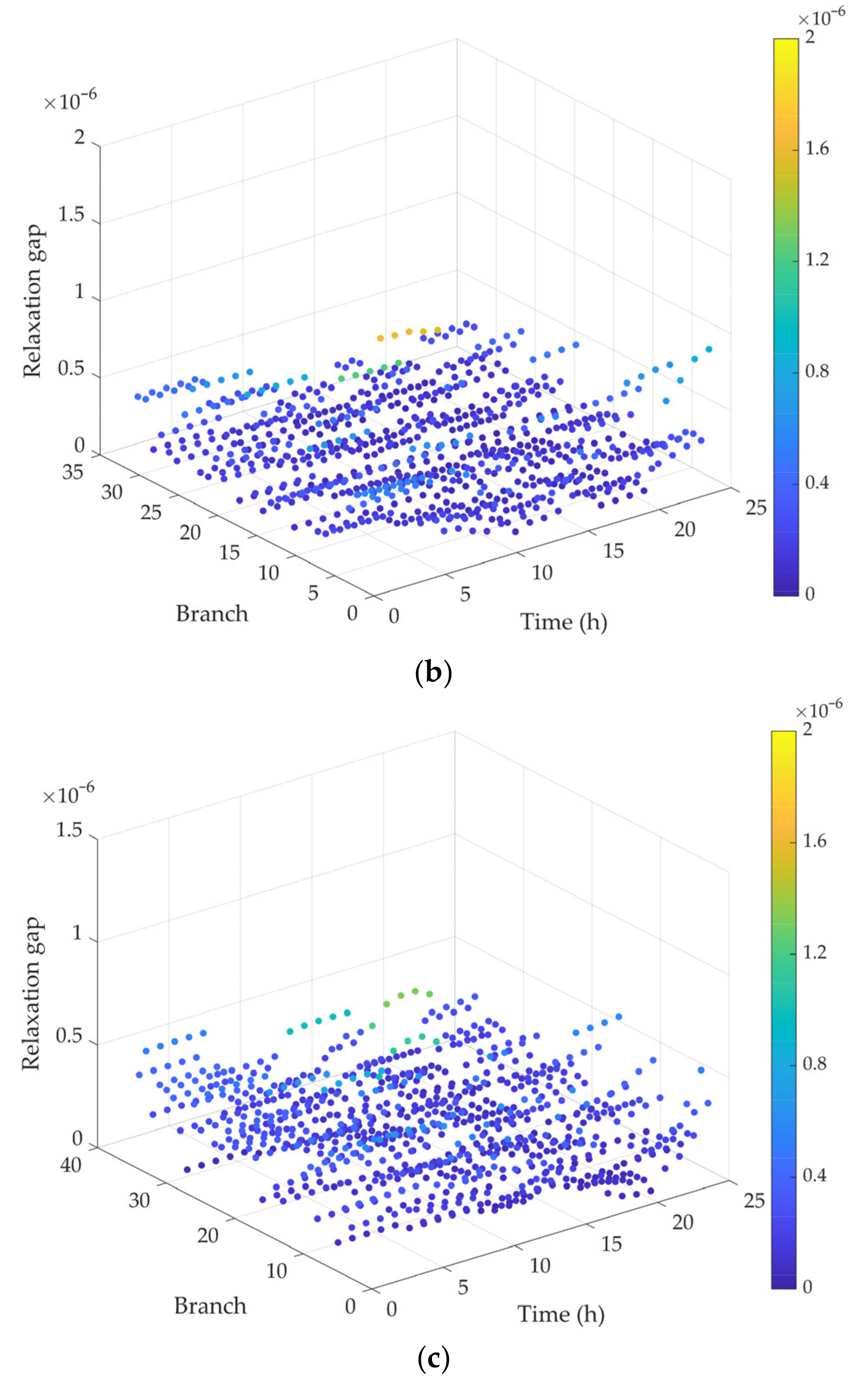
The rank-one constraint is relaxed during model solution, so it is necessary to analyze the solution accuracy of this relaxation. In fact, when the objective function is a strictly increasing function of the system’s injected currents, it is generally believed that the rank-1 constraint remains satisfied and the relaxation is exact [45]. However, if the objective function does not satisfy the strictly increasing condition, the SDP relaxation may become inexact, and the resulting solution could have a rank greater than 1. To evaluate the accuracy of the SDP relaxation in the proposed strategy—specifically, to assess how closely the matrix variable in Equation (19) approximates rank-1—the maximum two eigenvalues ${\alpha }_1$ and ${\alpha }_2$ ($\left|{\alpha }_1\right|\ge \left|{\alpha }_2\right|\ge 0$) of the matrix are computed, and their ratio $R=\left|{\alpha }_2\right|/\left|{\alpha }_1\right|$ is defined as the semidefinite relaxation gap. $R$ serves as an indicator of the accuracy of the rank-1 constraint relaxation. The smaller the value of $R$, the closer the matrix is to rank-1. A sufficiently small ratio indicates that relaxation achieves numerical exactness [46]. Otherwise, it may be necessary to strengthen the constraint by adding effective inequalities or by tightening variable bounds in the semidefinite program. The computed average semidefinite relaxation gaps for each branch of the three distribution networks under multiple scenarios are illustrated in Figure 12.

Figure 12. Semidefinite relaxation gaps for all branches of each network. (a) Semidefinite relaxation gaps of N1; (b) semidefinite relaxation gaps of N2; (c) semidefinite relaxation gaps of N3.

Figure 12 shows that the semidefinite relaxation gaps for all branches of each network are less than 1.0 × 10⁻⁵. Therefore, it can be concluded that the ranks of the matrices in Equation are numerically very close to rank-1, and the semidefinite relaxation in this case can be regarded as numerically exact. In other words, the SDP relaxation solution is also optimal for the original nonconvex problem. By employing the convex relaxation approach for the original problem, the constructed SDP model maintains convexity while ensuring solution accuracy.

4.5. Sensitivity Analysis of BES Investment Cost Coefficient

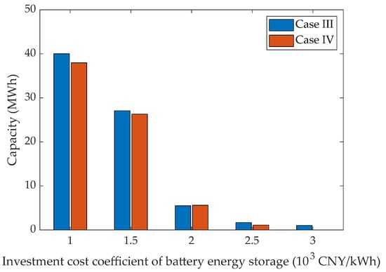
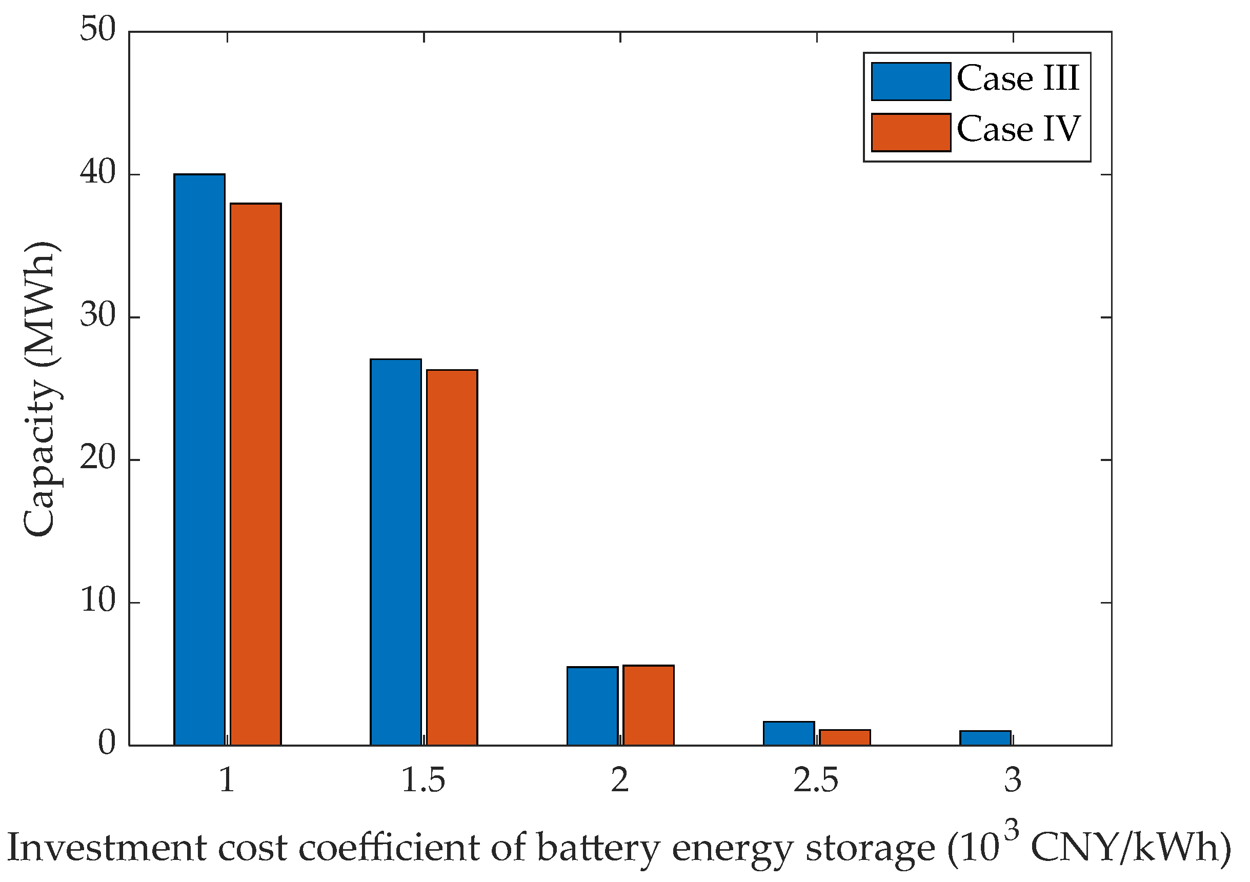
To further evaluate the robustness and economic adaptability of the proposed coordinated planning method, a sensitivity analysis was conducted regarding the unit investment cost coefficient of the battery energy storage, denoted as $c_{\mathrm{BES}}$. The BES investment cost varies from 1 × 10³ to 3 × 10³ CNY/kWh, while all other parameters remain unchanged. Table 16 summarizes the cost results for the independent planning scheme (Case III) and coordinated planning scheme (Case IV) with varying battery energy storage investment cost coefficients. Figure 13 shows the optimal total configuration capacity of the battery energy storage in E-SOP under different cases.

Table 16. Cost results with different battery energy storage investment cost coefficients.

${\mathit{c}}_{\mathit{B}\mathit{E}\mathit{S}}$	Case	Total Cost	Investment Cost	O&M Cost	Electricity Purchase Cost
1	Case III	37,593.1	9305.1	1858.8	26,429.2
	Case IV	37,494.9	9069.1	1835.5	26,590.3
1.5	Case III	39,555.5	8891.8	1818.1	28,845.6
	Case IV	39,377.3	8695.2	1798.8	28,883.3
2	Case III	40,216.0	5038.4	1439.8	33,737.8
	Case IV	39,952.7	4997.6	1435.7	33,519.4
2.5	Case III	40,396.2	4080.1	1345.7	34,970.4
	Case IV	40,193.3	3952.1	1333.1	34,908.1
3	Case III	40,468.6	3962.1	1334.1	35,172.4
	Case IV	40,216.4	3646.3	1303.1	35,267.0

Unit: The unit of $c_{\mathrm{BES}}$ is 10³ CNY/kWh. The unit of total cost, investment cost, O&M cost, and electricity purchase cost is 10³ CNY.

Figure 13. Total configuration capacity of battery energy storage with varying investment cost coefficients.

As shown in Table 16, the total planning cost of both schemes increases monotonically with the BES investment cost. Specifically, when the BES cost coefficient rises from 1 × 10³ to 3 × 10³ CNY/kWh, the total cost increases from 37.59 to 40.47 million CNY in the independent scheme and from 37.50 to 40.22 million CNY in the coordinated scheme. A more detailed decomposition of the cost components shows that the investment and operation and maintenance costs decrease as the BES cost increases, whereas the electricity purchase cost increases. This result suggests that when storage becomes more expensive, the optimization model tends to reduce the installed storage-related capacity and rely more heavily on grid electricity purchase. In other words, the planning outcome shifts from a strategy of extensively deploying energy storage to a more conservative investment strategy. The installed capacity results in Figure 13 also confirm this tendency. The optimal BES capacity is highly sensitive to its investment cost. In both cases, configuration capacity of BES decreases significantly as $c_{\mathrm{BES}}$ rises.

Furthermore, a comparative analysis between the two schemes reveals that the proposed coordinated planning (Case IV) consistently achieves lower total annual costs than the independent planning (Case IV) across the entire range of $c_{\mathrm{BES}}$. Table 16 shows that investment and O&M costs are consistently lower under coordinated planning than that under independent planning. Figure 13 also shows that the energy storage capacity configured under coordinated planning is generally smaller. This suggests that the cost improvement is mainly attributed to the cross-regional resource sharing enabled by the coordinated planning scheme, which allows the BES and other resources to be jointly configured and more efficiently utilized across different distribution networks. This effectively reduces redundant investment. As a result, the coordinated scheme consistently yields a lower total cost than the independent scheme, which confirms the robustness of the approach and highlights its practical value for multi-stakeholder distribution systems.

5. Conclusions and Prospects

In this paper, a coordinated planning model for a flexible interconnected distribution system is proposed and solved in a distributed manner using an improved ADMM algorithm. The primary conclusions can be summarized as follows:

(1)

Coordinated planning framework based on shared E-SOP proposed in this study significantly improves system economic efficiency while mitigating voltage imbalances. Not only does the maximum voltage imbalance across all distributed grids decrease to 2.00%, but the proposed coordinated planning also reduces the system’s total annual cost from 40,216.0 × 10³ CNY to 39,952.7 × 10³ CNY compared to independent planning. These savings stem from cross-regional resource sharing, which avoids redundant investment and achieves optimal utilization of PV generation and energy storage resources across power grids.

(2)

The distributed ADMM algorithm with an adaptive penalty factor update strategy offers an effective solution tool for multi-region coordinated planning. Compared with centralized methods, the distributed solution method achieves an optimality gap of less than 0.1% while protecting the data privacy of each distribution network. Compared with traditional ADMM algorithms, the proposed improved ADMM algorithm demonstrates good adaptability to different initial penalty factors, ensuring fast and stable convergence.

(3)

The cost-sharing mechanism based on Shapley values described in this paper provides a fair and reasonable approach to allocating cooperative costs among multiple stakeholders. While maximizing the overall benefits of the interconnected system, it also protects the interests of each participant, thereby enhancing the willingness of each region to participate in joint construction. This is important for the practical implementation of multi-region coordinated planning.

In addition, future work will expand the proposed framework in several promising directions:

(1)

In this paper, the model considers three typical scenarios to represent PV generation and load variations. The uncertainty of PV and load is not fully captured by this discrete-scenario-based approach. Future work will extend the model to a robust or distributionally robust optimization framework to better handle uncertainties.

(2)

The distributed optimization is implemented using an improved ADMM algorithm in this study. In future work, we will further examine other distributed algorithms beyond ADMM, including primal–dual methods, consensus-based approaches, and second-order distributed Newton-type methods. This will provide deeper insights into the trade-offs between convergence speed, communication burden, and solution quality across different distributed frameworks.

References

- Dong, F.; Hou, Y.; Li, W.; Wang, Y. Intelligent Decision-Making of Distribution Network Planning Scheme with Distributed Wind Power Generations. Int. J. Electr. Power Energy Syst. 2022, 136, 107673. [Google Scholar] [CrossRef] [Scilit]
- Vita, V.; Alimardan, T.; Ekonomou, L. The Impact of Distributed Generation in the Distribution Networks’ Voltage Profile and Energy Losses. In Proceedings of the 2015 IEEE European Modelling Symposium (EMS), Madrid, Spain, 6–8 October 2015; pp. 260–265. [Google Scholar]
- Fotopoulou, M.; Tsekouras, G.; Rakopoulos, D.; Kontargyri, V. Demand Response Optimization for the Enhancement of the Distribution System’s Operation. Sustain. Energy Grids Netw. 2025, 44, 102051. [Google Scholar] [CrossRef] [Scilit]
- Ma, K.; Fang, L.; Kong, W. Review of Distribution Network Phase Unbalance: Scale, Causes, Consequences, Solutions, and Future Research Directions. CSEE J. Power Energy Syst. 2020, 6, 479–488. [Google Scholar] [CrossRef] [Scilit]
- Gnacinski, P. Windings Temperature and Loss of Life of an Induction Machine under Voltage Unbalance Combined with Over- or Undervoltages. IEEE Trans. Energy Convers. 2008, 23, 363–371. [Google Scholar] [CrossRef] [Scilit]
- Kostic, M. Effects of Voltage Quality on Induction Motors’ Efficient Energy Usage. In Induction Motors—Modelling and Control; IntechOpen: London, UK, 2012; ISBN 978-953-51-0843-6. [Google Scholar]
- Yung, C. Stopping a Costly Leak: The Effects of Unbalanced Voltage on the Life and Efficiency of Three-Phase Electric Motors; Department of Energy, Office of Energy Efficiency and Renewable Energy: Washington, DC, USA, 2005. [Google Scholar]
- Zhang, Q.; Dehghanpour, K.; Wang, Z. Distributed CVR in Unbalanced Distribution Systems with PV Penetration. IEEE Trans. Smart Grid 2019, 10, 5308–5319. [Google Scholar] [CrossRef] [Scilit]
- Saurav, P.K.; Mansani, S.; Kayal, P. Multi-Faceted Sustainability Improvement in Low Voltage Power Distribution Network Employing DG and Capacitor Bank. Comput. Electr. Eng. 2024, 120, 109789. [Google Scholar] [CrossRef] [Scilit]
- Zhou, A.; Zhai, H.; Yang, M.; Lin, Y. Three-Phase Unbalanced Distribution Network Dynamic Reconfiguration: A Distributionally Robust Approach. IEEE Trans. Smart Grid 2022, 13, 2063–2074. [Google Scholar] [CrossRef] [Scilit]
- Jimenez, V.A.; Will, A.L.E.; Lizondo, D.F. Phase Reassignment for Load Balance in Low-Voltage Distribution Networks. Int. J. Electr. Power Energy Syst. 2022, 137, 107691. [Google Scholar] [CrossRef] [Scilit]
- Bloemink, J.M.; Green, T.C. Increasing Distributed Generation Penetration Using Soft Normally-Open Points. In Proceedings of the IEEE PES General Meeting, Minneapolis, MN, USA, 25–29 July 2010; pp. 1–8. [Google Scholar]
- Wang, C.; Song, G.; Li, P.; Ji, H.; Zhao, J.; Wu, J. Optimal Siting and Sizing of Soft Open Points in Active Electrical Distribution Networks. Appl. Energy 2017, 189, 301–309. [Google Scholar] [CrossRef] [Scilit]
- Tao, A.; Zhou, N.; Chi, Y.; Wang, Q.; Dong, G. Multi-Stage Coordinated Robust Optimization for Soft Open Point Allocation in Active Distribution Networks with PV. J. Mod. Power Syst. Clean Energy 2023, 11, 1553–1563. [Google Scholar] [CrossRef] [Scilit]
- Pamshetti, V.B.; Singh, S.; Thakur, A.K.; Singh, S.P.; Babu, T.S.; Patnaik, N.; Krishna, G.H. Cooperative Operational Planning Model for Distributed Energy Resources with Soft Open Point in Active Distribution Network. IEEE Trans. Ind. Appl. 2023, 59, 2140–2151. [Google Scholar] [CrossRef] [Scilit]
- Xiao, H.; Pei, W.; Li, K. Optimal Sizing and Siting of Soft Open Point for Improving the Three Phase Unbalance of the Distribution Network. In Proceedings of the 2018 21st International Conference on Electrical Machines and Systems (ICEMS), Jeju, Republic of Korea, 7–10 October 2018; pp. 2080–2084. [Google Scholar]
- Zhang, J.; Wang, T.; Liao, Z.; Tang, Z.; Wang, H.; Yue, J.; Shu, J.; Dong, Z. Flexible Interconnection Strategy for Distribution Networks Considering Multiple Soft Open Points Siting and Sizing. Electr. Power Syst. Res. 2025, 241, 111335. [Google Scholar] [CrossRef] [Scilit]
- Newton, C.; Lang, P.; Terry, S. Field Trial Results of Power Electronics in Low-Voltage Distribution Networks. In Proceedings of the CIRED—Open Access Proceedings Journal; Glasgow, UK, 2017; Volume 2017, pp. 184–188. [Google Scholar]
- Jiang, X.; Zhou, Y.; Ming, W.; Yang, P.; Wu, J. An Overview of Soft Open Points in Electricity Distribution Networks. IEEE Trans. Smart Grid 2022, 13, 1899–1910. [Google Scholar] [CrossRef] [Scilit]
- Marz, M.; Dickmander, D.; Johansson, F.; Irwin, G.; Sankar, S.; Copp, K.; Danielsson, J.; Holmberg, P.; Electranix; Manty, A.; et al. Converter Automatic Runback Utilizing Locally Measured Quantities; CIGRE Canada: Montreal, QC, Canada, 2014. [Google Scholar]
- Favre-Perrod, P.; Auberson, E.; Bernasconi, C.; Demierre, A.; Gavin, S.; Carpita, M.; Bifrare, A. Application of Soft-Open Points for the Interconnection of Neighbouring Low Voltage Distribution Networks. IET Conf. Proc. 2021, 2021, 1076–1080. [Google Scholar] [CrossRef] [Scilit]
- Li, P.; Ji, J.; Chen, S.; Ji, H.; Xu, J.; Song, G.; Zhao, J.; Wu, J.; Wang, C. Multi-Stage Expansion Planning of Energy Storage Integrated Soft Open Points Considering Tie-Line Reconstruction. Prot. Control Mod. Power Syst. 2022, 7, 45. [Google Scholar] [CrossRef] [Scilit]
- Diao, H.; Li, P.; Tu, C.; Che, L. Optimal Co-Planning of Multi-Port Soft Open Points and Energy Storage Systems for Improving Hosting Capacity and Operation Efficiency in Distribution Networks. IEEE Trans. Power Deliv. 2025, 40, 459–471. [Google Scholar] [CrossRef] [Scilit]
- Wang, P.; Li, H. Coordinated Planning of Soft Open Point and Energy Store System in Active Distribution Networks under Source-Load Imbalance. Electr. Power Syst. Res. 2024, 231, 110324. [Google Scholar] [CrossRef] [Scilit]
- Boyd, S.; Parikh, N.; Chu, E.; Peleato, B.; Eckstein, J. Distributed Optimization and Statistical Learning via the Alternating Direction Method of Multipliers. Found. Trends Mach. Learn. 2011, 3, 1–122. [Google Scholar] [CrossRef] [Scilit]
- Erseghe, T. Distributed Optimal Power Flow Using ADMM. IEEE Trans. Power Syst. 2014, 29, 2370–2380. [Google Scholar] [CrossRef] [Scilit]
- Lu, C.-F.; Liu, G.-P.; Cui, J. ADMM-Based Distributed Economic Dispatch Approach for Distributed Generators and Energy Storage Systems with Time-Varying Network. Control Eng. Pract. 2026, 167, 106635. [Google Scholar] [CrossRef] [Scilit]
- Zhang, T.; Pu, T.; Dong, L.; Yuan, X.; Mu, Y.; Jia, H. Distributed Reactive Power Optimization for Flexible Distribution Networks with Successive Relaxation Iteration Method. IEEE Trans. Sustain. Energy 2025, 16, 452–468. [Google Scholar] [CrossRef] [Scilit]
- Li, P.; Ji, H.; Wang, C.; Zhao, J.; Song, G.; Ding, F.; Wu, J. Optimal Operation of Soft Open Points in Active Distribution Networks under Three-Phase Unbalanced Conditions. IEEE Trans. Smart Grid 2019, 10, 380–391. [Google Scholar] [CrossRef] [Scilit]
- Lou, C.; Yang, J.; Vega-Fuentes, E.; Meena, N.K.; Min, L. Multi-Terminal Phase-Changing Soft Open Point SDP Modeling for Imbalance Mitigation in Active Distribution Networks. Int. J. Electr. Power Energy Syst. 2022, 142, 108228. [Google Scholar] [CrossRef] [Scilit]
- Std 141-1993; IEEE Recommended Practice for Electric Power Distribution for Industrial Plants. IEEE: New York, NY, USA, 1994; pp. 1–768. [CrossRef] [Scilit]
- IEEE Std 1159-2019 (Revis. IEEE Std 1159-2009); IEEE Recommended Practice for Monitoring Electric Power Quality. IEEE: New York, NY, USA, 2019; pp. 1–98. [CrossRef] [Scilit]
- Lanza, L.; Faulwasser, T.; Worthmann, K. Distributed Optimization for Energy Grids: A Tutorial on ADMM and ALADIN; The Institution of Engineering and Technology: Stevenage, UK, 2024; pp. 121–145. ISBN 978-1-78561-876-5. [Google Scholar]
- Sun, J.; Xi, H.; Yu, K.; Xiang, Y.; Qu, H.; Wu, L. Hierarchical Distributed Energy Interaction Management Strategy for Multi-Island Microgrids Based on the Alternating Direction Multiplier Method. Electronics 2025, 14, 4238. [Google Scholar] [CrossRef] [Scilit]
- Hong, M.; Luo, Z.-Q.; Razaviyayn, M. Convergence Analysis of Alternating Direction Method of Multipliers for a Family of Nonconvex Problems. In Proceedings of the 2015 IEEE International Conference on Acoustics, Speech and Signal Processing (ICASSP), South Brisbane, Australia, 19–24 April 2015; pp. 3836–3840. [Google Scholar]
- Xu, Z.; Figueiredo, M.; Goldstein, T. Adaptive ADMM with Spectral Penalty Parameter Selection. arXiv 2016, arXiv:1605.07246. [Google Scholar] [CrossRef] [Scilit]
- Shapley, L.S. A Value for N-Person Games. In The shapley Value: Essays in Honor of Lloyd S. Shapley; Roth, A.E., Ed.; Cambridge University Press: Cambridge, UK, 1988; pp. 31–40. ISBN 978-0-521-36177-4. [Google Scholar]
- Singh, V.P.; Ahmad, A.; Jagtap, K.M. Weighted Shapley Value: A Cooperative Game Theory for Loss Allocation in Distribution Systems. Front. Energy Res. 2023, 11, 1129846. [Google Scholar] [CrossRef] [Scilit]
- Schneider, K.P.; Mather, B.A.; Pal, B.C.; Ten, C.-W.; Shirek, G.J.; Zhu, H.; Fuller, J.C.; Pereira, J.L.R.; Ochoa, L.F.; de Araujo, L.R.; et al. Analytic Considerations and Design Basis for the IEEE Distribution Test Feeders. IEEE Trans. Power Syst. 2018, 33, 3181–3188. [Google Scholar] [CrossRef] [Scilit]
- Tian, Z.; Wu, W.; Zhang, B.; Bose, A. Mixed-Integer Second-Order Cone Programing Model for VAR Optimisation and Network Reconfiguration in Active Distribution Networks. IET Gener. Transm. Distrib. 2016, 10, 1938–1946. [Google Scholar] [CrossRef] [Scilit]
- Open Energy Data Initiative (OEDI). Available online: https://data.openei.org/ (accessed on 23 March 2026).
- Jia, Y.; Li, Q.; Liao, X.; Liu, L.; Wu, J. Research on the Access Planning of SOP and ESS in Distribution Network Based on SOCP-SSGA. Processes 2023, 11, 1844. [Google Scholar] [CrossRef] [Scilit]
- Ju, Y.; Li, H.; Yu, Z.; Yan, Y.; Zheng, L. Bi-Level Robust Capacity Planning of Micro-Grid Considering Multivariate Uncertainties and Reserve Demand. Power Syst. Technol. 2022, 47, 3343–3354. (In Chinese) [Google Scholar]
- Wohlberg, B. ADMM Penalty Parameter Selection by Residual Balancing. arXiv 2017, arXiv:1704.06209. [Google Scholar] [CrossRef] [Scilit]
- Dall’Anese, E.; Zhu, H.; Giannakis, G.B. Distributed Optimal Power Flow for Smart Microgrids. IEEE Trans. Smart Grid 2013, 4, 1464–1475. [Google Scholar] [CrossRef] [Scilit]
- Gan, L.; Low, S.H. Convex Relaxations and Linear Approximation for Optimal Power Flow in Multiphase Radial Networks. In Proceedings of the 2014 Power Systems Computation Conference, Wroclaw, Poland, 18–22 August 2014; pp. 1–9. [Google Scholar]
Disclaimer/Publisher’s Note: The statements, opinions and data contained in all publications are solely those of the individual author(s) and contributor(s) and not of MDPI and/or the editor(s). MDPI and/or the editor(s) disclaim responsibility for any injury to people or property resulting from any ideas, methods, instructions or products referred to in the content. |
© 2026 by the authors. Licensee MDPI, Basel, Switzerland. This article is an open access article distributed under the terms and conditions of the Creative Commons Attribution (CC BY) license.