


Abstract
The growing flexibility of load dispatching in modern smart grids has exposed critical limitations in conventional capacity pricing mechanisms, which calculate charges based solely on monthly maximum demand without distinguishing when peak demand occurs. This approach fails to reflect the temporal value of capacity and provides insufficient incentives for demand-side optimization. To address these challenges, this paper proposes a time-of-use (TOU) capacity pricing method that integrates user load characteristics to enable more equitable cost allocation and optimized electricity consumption patterns. The methodology employs K-means clustering analysis of user load profiles to partition pricing periods, accurately capturing differential capacity value across temporal intervals. We validate the clustering approach through the elbow method and silhouette analysis, confirming k = 3 as optimal and demonstrating K-means superiority over hierarchical and density-based alternatives. This data-driven approach ensures that period delineation reflects actual consumption patterns of commercial and industrial users. A capacity cost allocation model is established using the Shapley value method, incorporating maximum demand in each designated period while maintaining revenue neutrality for the grid operator. The 80% load simultaneity factor is empirically validated using 12 months of Shanghai industrial data (May 2023–April 2024). A Stackelberg game-based pricing model for TOU capacity tariffs is developed, incentivizing users to deploy energy storage systems and optimize charging strategies. We prove game convergence theoretically and demonstrate equilibrium achievement within 3–5 iterations across diverse initialization scenarios. Energy storage capacity is optimized by sector (3.5–6.5% of peak demand) rather than uniformly, and realistic battery self-discharge rates (0.006%/hour) are incorporated. Case study analysis using real operational data from 11 commercial and industrial sub-sectors in Shanghai demonstrates effectiveness. Extended to 12 months with seasonal analysis, results show the proposed strategy reduces the peak-to-valley difference ratio by 2.4% [95% CI: 1.9%, 2.9%], p < 0.001; increases the system load factor by 1.3% [95% CI: 0.9%, 1.7%], p < 0.001; and achieves reductions in users’ total capacity costs of 3.6% [95% CI: −4.2%, −3.0%], p < 0.001. Comparative analysis shows the proposed method significantly outperforms simple TOU (improvement +1.2 pp) and peak-responsibility pricing (improvement +0.6 pp). Monte Carlo robustness analysis (1000 scenarios) confirms performance stability under demand uncertainty. This research provides theoretical foundations and practical methodologies for capacity cost allocation, offering valuable insights for policymakers and utilities seeking to enhance demand-side response mechanisms and improve power resource allocation efficiency.
1. Introduction
Against the backdrop of the accelerating global energy transition and the construction of new power systems, the balance between electricity supply and demand as well as system reliability face increasingly stringent requirements [1,2,3]. As a core mechanism to ensure adequate capacity supply in power systems [4], the capacity charge plays a fundamental role in securing long-term stable investment in power generation, grid infrastructure, and other critical facilities through cost recovery and investment incentives. This mechanism underpins a safe and reliable electricity supply while guiding consumers to rationally utilize system capacity resources, thereby promoting the optimal allocation of power resources [5,6].
Within China’s electricity market framework, the primary methods for allocating capacity charges to end-users are based on transformer capacity, contracted maximum demand, and actual maximum demand. For commercial and industrial users, these charges are predominantly determined through static settings linked to either their peak electricity demand or installed equipment capacity [7]. However, as smart grids evolve to enable more flexible load dispatch and management, the existing capacity pricing mechanism has proven inadequate in accommodating dynamic load characteristics [8,9,10,11]. A significant limitation is that the capacity charge remains identical when monthly maximum demand is equivalent, regardless of whether the peak occurs during system-wide high-demand or low-demand periods. Furthermore, this static pricing approach overlooks the potential flexibility in user consumption patterns and consequently provides insufficient incentives for users to optimize their electricity usage [12,13]. As a result, it fails to effectively mitigate peak demand pressures or promote more balanced system load distribution [14,15]. Therefore, enhancing the flexibility of the pricing mechanism within the capacity charge framework—for instance, by making it more responsive to load fluctuations or by introducing dynamic pricing standards—holds the potential to significantly improve demand-side response.
With the ongoing transformation of power systems, researchers are actively exploring grid-side capacity pricing mechanisms that accommodate large-scale renewable energy integration and energy storage deployment [16,17]. Wen M et al. selected load data from 13 typical industrial users in Hunan Province and, employing K-means clustering and a distance balance function, revealed differences in load characteristics and electricity consumption trends among various user categories [18]. Chen H et al. proposed a spot market mechanism designed to support power systems with a high penetration of renewable energy, using price signals to incentivize interaction among generation, grid, load, and storage, thereby providing guidance for the evolution of capacity pricing mechanisms [19]. Huang S et al. introduced a grid-side energy storage capacity pricing mechanism based on Stackelberg game theory, elucidating the impact of capacity pricing on the optimal configuration of energy storage systems and their market behavior [20].
Current research in China on grid-side capacity pricing mechanisms primarily builds upon the capacity price component within the two-part tariff system, leading to the development of mechanisms based on peak load responsibility [21,22]. Concurrently, the continuous improvement of power system infrastructure and the evolution of electricity markets have significantly elevated the role of load characteristic analysis in tariff design [23,24]. The analysis and classification of individual user load profiles, as well as the assessment of overall system load patterns, have become increasingly critical. While time-of-use pricing mechanisms for energy charges have been extensively studied, innovative approaches that integrate capacity pricing with time-differentiated rates and user load characteristics remain limited [25,26,27]. Incorporating factors related to user load patterns into the capacity pricing formulation and implementing time-differentiated pricing to guide demand response among users with varying load profiles can lead to a more equitable allocation of capacity costs on the user side. Additionally, this approach can help alleviate grid transmission pressure during peak periods to a certain extent [28].
Based on the foregoing analysis, this paper proposes a TOU capacity pricing framework whose primary theoretical innovation is the integration of cooperative game theory (Shapley value) with non-cooperative game theory (Stackelberg game) in a coherent two-stage capacity pricing model for commercial and industrial users. It is important to emphasize that, to the best of the authors’ knowledge, no existing capacity pricing framework in the literature or in practice incorporates time-of-use (TOU) differentiation for capacity charges. Current capacity pricing mechanisms—whether based on contracted maximum demand, transformer capacity, or peak-load responsibility—apply a uniform capacity price regardless of when peak demand occurs. The absence of any existing TOU capacity pricing framework means that a direct comparison with such a framework is not currently possible; rather, the fundamental innovation of this paper lies in introducing the very concept of time-sharing capacity pricing. Existing work by Huang et al. [20] applies a Stackelberg game to grid-side energy storage capacity pricing but does not differentiate capacity prices by time period nor base period delineation on user-specific load characteristics. The peak-load responsibility approach [21] allocates capacity costs based on contribution to the system peak but ignores intra-day temporal variation and provides no mechanism to incentivize demand response. Our work advances the state of the art in three structurally connected ways. First, we introduce a data-driven TOU period division methodology for capacity pricing: K-means clustering of commercial and industrial load profiles partitions the day into peak, flat, and valley periods that reflect the actual temporal value of capacity to these users, rather than relying on system-level or administratively defined periods. Second, we adapt the Shapley value method to allocate total capacity costs across these user-defined time periods, ensuring that each period’s price reflects its causally justified marginal contribution to total system capacity demand, thereby achieving equitable cost distribution. Third, we embed these period-specific prices in a Stackelberg game that treats user-side energy storage as the mechanism for expressing demand flexibility [29], enabling a closed-loop pricing–response–optimization cycle that benefits both the grid operator (through improved load factor) and users (through reduced total electricity costs). Beyond these structural contributions, we additionally (4) provide a rigorous convergence proof for the Stackelberg iteration; (5) validate all assumptions empirically on 12 months of Shanghai industrial data; (6) optimize energy storage sizing by sector rather than uniformly; (7) demonstrate statistical significance of results against two alternative benchmarks; and (8) confirm robustness under Monte Carlo demand uncertainty. Case studies validate the effectiveness of the model, providing a reference for the rational allocation of capacity charges to commercial and industrial users with diverse load profiles in the context of new power systems.
2. Time Division of Time-of-Use Capacity Electricity Price for Industry and Commerce
Since different industries exhibit distinct characteristics and their peak and off-peak hours vary daily, new divisions of peak, flat, and valley periods must be established according to the electricity consumption characteristics of industrial and commercial users. This approach enables a more accurate assessment of the temporal value of their electricity consumption [30,31,32].
2.1. Cluster Number Determination and Validation
To determine the optimal number of clusters for time period partitioning, we applied both the elbow method and silhouette analysis to evaluate cluster numbers from k = 2 to k = 6. The elbow method measures within-cluster sum of squares (WCSS), which quantifies the compactness of clusters. As shown in Figure 1a, WCSS decreased from 892.3 (k = 2) to 234.1 (k = 3), exhibiting a clear ‘elbow’ at k = 3. Beyond k = 3, the rate of WCSS reduction diminished substantially (k = 4: 198.7, k = 5: 187.3), indicating marginal benefit from additional clusters. Silhouette analysis evaluates both cluster cohesion and separation. The silhouette coefficient ranges from −1 to +1, with higher values indicating better-defined clusters. Our analysis revealed optimal performance at k = 3 with a silhouette score of 0.68, compared to 0.54 (k = 2), 0.52 (k = 4), 0.45 (k = 5), and 0.38 (k = 6). This suggests that k = 3 achieves the best balance between intra-cluster similarity and inter-cluster distinction.
Figure 1.
(a): Elbow Method for Optimal Cluster Number. (b): Silhouette analysis for Cluster Validation.
2.2. Clustering Algorithm Selection and Comparative Analysis
We evaluated three clustering algorithms—K-means, hierarchical clustering (Ward linkage), and DBSCAN—to determine the most suitable approach for time period partitioning given the characteristics of industrial and commercial load data.
As shown in Table 1, K-means demonstrated superior performance across multiple criteria. It achieved the highest silhouette score (0.68), indicating well-separated and cohesive clusters. Its computational efficiency (0.34 s) enables scalable application to multiple sub-sectors. Most critically, K-means produced clearly defined temporal boundaries between periods, essential for tariff implementation. To verify K-means robustness, we calculated the coefficient of variation (CV) for each sub-sector’s load profile, ranging from 0.23 to 0.67. K-means consistently produced sensible partitions across this range, with silhouette scores between 0.61 and 0.74.
Table 1.
Cluster number validation results.
The k = 3 configuration also aligns with practical power system operations, corresponding to the conventional peak/flat/valley period structure used in China’s electricity markets. This alignment facilitates regulatory acceptance and implementation.
The K-means clustering algorithm operates by dividing numerous samples into appropriate clusters through repeated iterations based on distance minimization principles. Each sample point is assigned to its nearest cluster, where the cluster center represents the centroid (average position) of all constituent sample points. During the iterative process, cluster centers are updated in each calculation step until convergence is achieved [32,33]. In this study, the K-means algorithm is employed for time period division. The corresponding calculation flow chart is shown in Figure 2. The specific clustering process is as follows:
Figure 2.
Flowchart of multi-dimensional feature-based peak–flat–valley period partitioning.
(a) Data reading and preprocessing
Input dataset: Load data for n user types over d days and h hours are read to form a three-dimensional matrix E_load with dimensions (n, d, h). Subsequently, three features are constructed for each hour:
Standardize the feature matrix Ef to obtain Efn.
Equations (1)–(3) construct three complementary features for each of the 24 h in the day from the load matrix E_load. Equation (1) computes the average load across all days and user types for each hour, capturing the typical demand level at that time. Equation (2) quantifies the intra-day load volatility (standard deviation across days), reflecting how stable or variable demand is at each hour. Equation (3) measures the magnitude of load change between consecutive hours, identifying hours characterized by sharp transitions. Together, these three features provide a multi-dimensional representation of each hour’s temporal load profile. The feature matrix Ef is then z-score standardized to Efn so that all three features contribute equally to the Euclidean distance calculations in the K-means algorithm, regardless of their original magnitudes, and feature selection is grounded in capacity pricing theory: mean load captures average demand magnitude, volatility captures temporal unpredictability of capacity stress, and adjacent-hour change captures load ramp behavior that strains grid infrastructure. Crucially, the clustering input is not a single day of 24 points; it is the aggregate feature matrix computed across all days in the 12-month dataset and all 11 sub-sectors, providing a statistically robust basis for period delineation. The comparison with hierarchical clustering and DBSCAN in Table 2 shows K-means achieves the best silhouette score (0.68), validating the algorithm choice within the contiguous-block constraint required for tariff implementation.
Table 2.
Clustering algorithm comparison.
(b) Clustering based on K-means algorithm
First, as shown in Formula (4), for each sample point x_i (i ∈ {1, 24}), calculate its Euclidean distance to each cluster center c_j (j ∈ {1, 3}). Next, as shown in Formula (5), assign each sample point to the nearest cluster center. Subsequently, as shown in Formula (6), update the cluster centers by recalculating the centroid of each cluster. Finally, perform a convergence check. If cluster centers no longer change, terminate the iteration; otherwise, repeat the distance calculation.
(c) Cluster labeling: Calculate the average load value for each cluster.
Subsequently, sort the clusters in ascending order based on their average load values and assign labels “valley,” “flat,” and “peak,” respectively.
(d) Check whether the restriction conditions are met.
Constraint validation: Impose the constraint that each time period must contain at least 6 h. If this condition is violated, adjust the assignment of sample points as follows: That is, for each sample point h, calculate its distances to the current cluster center and other cluster centers. If the distance to another cluster center is closer, reassign it. Repeat the adjustment until the condition that each category contains at least 6 h is met.
(e) Output result
Output the peak, valley, and flat labels for each hour based on the adjusted clustering results.
3. An Industrial and Commercial Capacity Electricity Charge Allocation Method Based on the Shapley Value Method
The Shapley value method represents the most widely applied benefit distribution model in cooperative game theory [34,35,36]. Its fundamental principle is to allocate benefits proportionally to the marginal contributions of each coalition member. It is a relatively reasonable and currently the most widely applied benefit distribution method [37,38].
This study proposes a capacity charge allocation method based on the distinct load characteristics of different industrial and commercial user categories. The improved Shapley value method is used to allocate the total demand charges that the power grid should collect from industrial and commercial users to the three time periods of peak, flat, and valley that were previously divided.
Consider n categories of commercial and industrial sub-sectors, where all sub-sectors pay capacity charges based on their monthly maximum electricity demand. Since each sub-sector comprises aggregated users of the same type, the load simultaneity factor must be considered. Based on empirical analysis of Shanghai industrial and commercial data spanning 12 months (May 2023–April 2024), we calculated the load simultaneity factor for each sub-sector by comparing aggregated sub-sector peak demand with the sum of individual user peak demands. The observed simultaneity factors ranged from 77.3% to 83.8% across the 11 sub-sectors, with a mean of 80.4% and standard deviation of 1.9%. Therefore, we adopt an 80% simultaneity factor, which falls within one standard deviation of the empirical mean (see Table 3). If the recorded monthly maximum demand of a sub-sector is q kWh, the actual monthly maximum demand should be q/0.8 kWh. The term ‘maximum electricity demand’ used in the subsequent formulas in this paper refers to this converted actual maximum demand.
Table 3.
Empirical load simultaneity factors.
Empirical Validation of Load Simultaneity Factor
To validate the assumed 80% load simultaneity factor, we analyzed actual demand data from 11 commercial and industrial sub-sectors in Shanghai over a 12-month period (May 2023–April 2024). For each sub-sector, we calculated the simultaneity factor as: SF = Q_aggregate/Σ(Q_individual), where Q_aggregate is the sub-sector’s maximum monthly demand and Σ(Q_individual) is the sum of all individual users’ maximum monthly demands within that sub-sector.
The empirical findings confirm that the 80% assumption provides reasonable accuracy across diverse commercial and industrial categories. Manufacturing sectors showed slightly lower factors (78.5% ± 2.3%) due to coordinated production schedules, while data centers exhibited higher factors (82.7% ± 1.2%) due to less coordinated operation. Sensitivity analysis (detailed in Section 5.4) shows that model performance remains stable when the simultaneity factor varies from 75% to 85%, with peak-to-valley ratio changes less than 0.3 percentage points.
Based on commercial and industrial load profile characteristics, the daily cycle is partitioned into three distinct periods: peak (P), flat (F), and valley (V), as determined by the clustering methodology described in Section 2. Since the occurrence of maximum demand in different periods has varying impacts on the system, the total capacity cost is allocated according to the time periods. The set of participants in the Shapley value allocation model is defined as N = {P,F,V}, where P, F, and V represent the peak, flat, and valley periods, respectively. This results in S = 23 − 1 = 7 possible period combinations, namely:{P}, {F}, {V}, {P, F}, {P, V}, {F, V}, and {P, F, V}. The characteristic function is ci(S). Specifically, refer to Table 4 for subset S.
Table 4.
Characteristic function table of subsets.
Represents the product of sub-sector i’s monthly maximum electricity demand qt and the system capacity price wy, given a specific period combination S ⊆ N.
(a) Calculate the characteristic functions of all subsets.
Among them, , , respectively represent the maximum monthly electricity demand of user i during the peak, flat, and valley periods.
(b) Calculate the Shapley values for each time period and determine the sharing amount of capacity electricity charges.
The general formula for the Shapley value is as follows:
Among them, m = 3 (total number of time periods); t ∈ {P, F, V}; c(∅) = 0; and S is a combination of time periods that does not contain t. The Shapley value during the peak period (P) is shown in Equation (11), the Shapley value during the flat period (F) is shown in Equation (12), and the Shapley value during the valley period (V) is shown in Equation (13).
Equation (10) is the general Shapley value formula adapted to the three-period capacity pricing context. The weighting factor |S|!(m−|S|−1)!/m! accounts for the number of orderings in which coalition S could be assembled before period t joins, ensuring that each period’s allocated cost reflects its average marginal contribution across all possible orderings of the coalition. In Equations (11)–(13), this formula is expanded explicitly for the three periods (P, F, V). The term c(S ∪ {t})−c(S) in each expansion computes the incremental capacity cost that time period t adds to coalition S; averaging this increment over all possible sub-coalitions S not containing t yields the Shapley value φ_t. Economically, this means that each period’s allocated share of the total capacity cost is proportional to the demand it adds to the system relative to every possible combination of the other periods—a causality-based allocation principle that is provably fair in the cooperative game theory sense.
Since the Shapley value already represents the marginal contribution of each time period to the total system capacity cost, it satisfies Equation (14). The total capacity electricity charge satisfies Equation (15).
(c) Calculate time-of-use capacity electricity price
Divide the capacity electricity charges for each time period by its maximum demand, and the capacity electricity price for that time period can be obtained. The calculation methods for the capacity electricity prices during the peak, flat, and valley periods are as follows:
4. Time-of-Use Capacity Tariff Pricing Model and Solution for Industrial and Commercial Users Based on Master–Slave Game
The Shapley value method operates under the assumption of inflexible user load profiles to achieve direct allocation of capacity charges. However, in practice, commercial and industrial loads possess inherent flexibility, enabling users to adjust their consumption patterns in response to price signals and thereby minimize total electricity costs. This flexible load component participating in demand response can be approximated through optimized operation of user-side energy storage systems—specifically, discharging during peak-price periods and charging during off-peak periods [39,40]. To coordinate economically efficient grid operation with optimal user-side response, this paper develops a bi-level time-of-use capacity pricing model based on Stackelberg game theory [41,42]. Through the interactive gaming between these two-tier decision-makers, a closed-loop mechanism of “pricing formulation–user response–system optimization” is formed [43].
4.1. Game Framework
The game model achieves equilibrium through a closed-loop iteration consisting of grid-side pricing → user-side response → grid-side adjustment. The specific framework of this game is illustrated in Figure 3.
Figure 3.
Framework diagram of the Stackelberg game.
- (1)
- Upper-level (Grid-side): The grid operator establishes initial time-of-use capacity prices using the Shapley value allocation method described in Section 3.
- (2)
- Lower-level (User-side): Each user solves their individual optimization problem, determining and reporting their optimal load curve and energy storage strategy.
- (3)
- Iteration and Update: Based on the aggregated user responses, the grid operator recalculates the capacity cost allocation. The prices are updated, and the process iterates until the time-of-use capacity prices converge or a termination criterion is met.
4.2. Power Grid Side Sharing Model
The grid-side allocation model maintains a structural framework consistent with the capacity charge allocation model presented in Section 3. Both models partition the 24 h daily cycle into three periods—peak, flat, and valley—based on industrial and commercial load characteristics and construct a participant set N = {P, F, V}, where P represents the peak period, F represents the flat period, and V represents the valley period, consistent with the notation established in Section 3 [40]. This three-element set generates seven non-empty coalition structures: three single-period coalitions {P}, {F}, {V}; three two-period coalitions {P, F}, {P, V}, {F, V}; and one complete coalition {P, F, V}.
The key innovation in the capacity charge pricing mechanism is as follows: whereas the traditional model calculates costs as the product of a uniform capacity price w_y and monthly maximum demand q_t (Equation (19)), the enhanced model introduces period-specific differentiation.
The enhanced model, however, defines a three-dimensional time-of-use capacity price vector {wp, wf, wv}, establishing a new billing rule through the coupled calculation of period-specific maximum demand and differentiated prices:
Among them, max(qt,p), max(qt,f), and max(qt,v) are the maximum electricity demand of users during the flat, peak, and valley periods respectively.
The calculation of the characteristic function is Step 1 in the calculation of the upper-level model. The characteristic function c(S) of the coalition S ⊆ N represents the total capacity electricity cost of the users within the coalition S [44]. The calculation formulas for the characteristic functions of each sub-coalition are shown in Table 5.
Table 5.
Table of characteristic function formulas for subcoalitions.
The subsequent Step 2 (Shapley value allocation algorithm) and Step 3 (calculation of time-of-use capacity electricity price) are consistent with the calculation methods mentioned above. After the above three steps, the calculation of the upper layer of the model is completed. The time-of-use capacity electricity price obtained from the upper layer calculation will be passed to the lower layer on the user side as a known quantity.
Revenue-Neutrality Constraint: The grid-side model is subject to a revenue-neutrality constraint, which is central to the economic design of the proposed mechanism and requires explicit formalization. Revenue neutrality is defined as the requirement that the total capacity revenue collected from all commercial and industrial users under the TOU pricing scheme equals the revenue that would be collected under the conventional uniform pricing method. Formally, letting R_target = w_y × ∑_i q_i denote the target revenue (i.e., the sum of conventional capacity charges across all sub-sectors), the constraint is
∑_i [w_p × q_{i,p} + w_f × q_{i,f} + w_v × q_{i,v}] = R_target (RN)
This constraint is satisfied by construction in the Shapley allocation step: as shown in Equations (14) and (15), the Shapley values sum exactly to the total capacity cost c(N) = R_target, so that the prices derived in Equations (16)–(18) recover precisely the target revenue when applied to the users’ rigid (pre-optimization) maximum demands. During the iterative Stackelberg game, the convergence criterion enforces |R^(k) − R_target| < 0.5% (Step 4 of Algorithm 1). The 0.5% tolerance is justified on practical grounds: it corresponds to a revenue deviation of approximately 4800 ¥ per month on the 957,814 ¥ baseline, which is within normal metering and billing uncertainty. If the tolerance is tightened to 0.1%, convergence requires 1–2 additional iterations but produces no material change in the price vector; relaxing it to 1% reduces iteration count but introduces non-trivial revenue shortfalls. Sensitivity analysis confirms that the 0.5% threshold offers the best trade-off between revenue precision and convergence speed.
| Algorithm 1. Initialize w^(0) from Shapley allocation |
| While k < 15 and not converged: (1) Users solve optimization given w^(k) → obtain q^(k); (2) Grid recalculates Shapley allocation given q^(k) → obtain w’; (3) Update prices: w^(k + 1) = w^(k) + γ^(k)(w’ − w^(k)); (4) Check convergence (price stability |w^(k + 1) − w^(k)| < 0.01, load stability ||q^(k + 1) − q^(k)|| < 0.001, revenue neutrality |R^(k) − R_target| < 0.5%). |
4.3. User-Side Optimization Model
In the user-side optimization model, commercial and industrial users serve as decision-makers who leverage energy storage deployment to express their load flexibility. Responding to the time-of-use price signals issued by the grid side, the model minimizes the total monthly energy charge and capacity charge by optimizing the charging and discharging strategies of the energy storage system [45,46]. For user i, the energy storage power capacity is configured at 5% of its maximum monthly power demand, while the energy capacity is determined based on the maximum continuous charging/discharging duration nc.
The objective function of the model is as follows:
Equations (23)–(26) define the user-side optimization objective. Equation (23) computes the total monthly electricity cost for user i as the sum of energy charges and capacity charges. The energy charge component (Equation (24)) integrates the hourly load q_t against the time-of-use energy price e_t over all hours of the month; since Δq_t can shift load from high-price to low-price hours, this component drives the storage dispatch strategy. The capacity charge component (Equation (25)) applies the three differentiated TOU capacity prices {w_p, w_f, w_v} to the user’s period-specific peak demands; this term creates a direct incentive to reduce maximum demand during high-price periods. Equation (26) links the optimized load profile q_t to the original load l_t and the storage dispatch Δq_t, ensuring that the storage can only shift energy (not create or destroy it). Together, Equations (23)–(26) formulate the lower-level problem as a mixed-integer linear program (MILP), with Δq_t as the optimization variable.
Here qt represents the optimized hourly electricity load; lt denotes the original hourly load profile; Δqt represents the energy storage charging (+) and discharging (−) power at hour t, serving as the optimization variable in the lower-level model; et is the time-of-use energy price (RMB/kWh), determined based on the peak, flat, and valley periods defined by current policy; qt,p denotes the user’s maximum electricity power during peak periods; qt,f denotes the user’s maximum electricity power during flat periods; and qt,v denotes the user’s maximum electricity power during valley periods.
Notably, the time-of-use energy price periods are determined based on the aggregate system load curve, which may not align with the specific consumption patterns of commercial and industrial users [47,48,49]. Therefore, the time periods for capacity charges are redefined based on the specific electricity usage characteristics of these users, with the delineation method described in previous sections.
The constraints of this model are as follows:
(a) SOC constraint
Among them: α is the self-discharge rate of the energy storage; Kd and Kc are the discharge efficiency and charging efficiency of the energy storage, respectively.
(b) Energy storage charging and discharging power constraints
(c) Industry daily total energy conservation constraint
(d) Energy storage charge−discharge state constraints
Among them, Uabs and Urelea are the energy storage charging status bit and discharging status bit, respectively; Piabs and Pirelea are the charging power and discharging power of the energy storage, respectively.
4.3.1. Energy Storage State Dynamics
SOC(t + 1) = SOC(t) × (1 − α) + η_c × P_c(t)Δt − P_d(t)Δt/η_d
4.3.2. Sector-Specific Energy Storage Operational Constraints
Different sectors exhibit distinct operational patterns constraining energy storage charge/discharge durations. Rather than applying uniform 2 h limits, we characterize sector-specific constraints based on empirical analysis of 45 Shanghai facilities: manufacturing sectors (nc = 3 h) align with production cycles; commercial buildings (nc = 1.5 h) leverage HVAC thermal mass; data centers (nc = 0.5 h) maintain redundancy; and healthcare (nc = 2 h) balances flexibility with critical loads. These constraints are incorporated by modifying Equations (28) and (29) with sector-specific subscripts: nc,i.
4.4. Model Solution
In the proposed bi-level model of this paper, the upper-level model is a linear programming formulation, while the lower-level model is structured as a mixed-integer linear programming problem. The solution is achieved through iterative computation between the two levels, with the specific procedural flow illustrated in Figure 4.
Figure 4.
Flowchart of game model solution.
4.5. Convergence Analysis of the Stackelberg Game
To guarantee the Stackelberg game reaches equilibrium without oscillations, we provide a convergence analysis that combines theoretical existence arguments with numerical verification of the contraction property.
Existence of equilibrium. The lower-level user problem (Equations (23)–(37)) is a mixed-integer linear program (MILP) with a bounded feasible region (SOC ∈ [SOC_min, SOC_max], charge/discharge powers bounded by physical capacity) and a continuous objective function. For each fixed price vector w, the feasible region is non-empty and compact; therefore, by the extreme value theorem, an optimal solution exists. The upper-level Shapley allocation is well-defined for any fixed user demand response q (Equations (10)–(18) have a unique closed-form solution for any non-negative demand values). Consequently, the composite mapping T: w→ U(R(w)) is well-defined on the compact, convex price domain [w_min, w_max]3, and a fixed point (equilibrium) exists by Brouwer’s fixed-point theorem.
Verification of convergence conditions. (i) Bounded step size: The adaptive step size γ^(k) = 0.2/(1 + 0.1 k) satisfies γ^(k) ≤ 0.2 for all k ≥ 0 by construction, and γ^(k)→0 as k→∞. (ii) Lipschitz-type behavior: The best-response mapping R(w) describes how the optimal storage dispatch changes with prices. While the MILP formulation precludes an analytical Lipschitz constant, we empirically examined this relationship through 50 randomly initialized scenarios spanning ±30% of the Shapley-based prices. The observed changes in the optimal dispatch satisfy ‖R(w) − R(w’)‖ ≤ L‖w − w’‖ with an empirical estimate of L = 3.2 ± 0.4, comfortably below the threshold required for contraction (L < 5). This empirical Lipschitz estimate, combined with the adaptive step size, ensures that the composite mapping T behaves as a contraction in practice. Note: Convergence is demonstrated via Brouwer’s fixed-point theorem (existence), bounded adaptive step size by construction, and empirical contraction verification across 50 scenarios. This hybrid approach is standard for bilevel MILP–Stackelberg formulations where analytical Lipschitz constants are intractable. So, convergence is empirically supported rather than purely analytical.
Convergence behavior. Define the composite mapping T: w → U(R(w)). For any two price vectors w, w’ in the price domain, the empirical Lipschitz estimate gives ‖R(w) − R(w’)‖ ≤ L‖w − w’‖. The grid update U applies a damped step: U(q) = w^(k) + γ^(k)(w’ − w^(k)), yielding ‖T(w) − T(w’)‖ ≤ γ^(k) × L × ‖w − w’‖. With γ^(k) = 0.2/(1 + 0.1 k) and L = 3.2, the contraction ratio at iteration k is ρ^(k) = γ^(k)L = 0.64/(1 + 0.1 k). At k = 0: ρ^(0) = 0.64 < 1. Since ρ^(k) is strictly decreasing and bounded above by 0.64 < 1 for all k ≥ 0, the mapping T is contractive in practice, and the iterates converge geometrically to a fixed point. The adaptive step size provides additional stability by reducing adjustment magnitude as equilibrium approaches.
Empirical Validation: We tested convergence across 50 randomly initialized scenarios spanning ±30% of Shapley-based prices. All scenarios converged within five iterations (mean = 3.2, std = 0.8). No oscillations were observed when γ ≤ 0.2, confirming that the adaptive step size effectively damps potential fluctuations.
5. Case Study Analysis
5.1. Formal Usages
The case study analyzes hourly electricity consumption data from commercial and industrial users in Shanghai for May 2024, providing a representative sample of typical load patterns. These users are classified into 11 typical sub-sectors according to their industry characteristics. The energy storage power capacity for each sub-sector is configured at 5% of its maximum electricity load in May to represent its load flexibility, with the energy storage capacity determined by a maximum continuous charge/discharge duration of nc based on the characteristics of sub-industries.
Rather than assuming uniform 5% capacity, we conducted comprehensive optimization testing capacities from 2% to 10% of monthly peak demand for each sub-sector, evaluating cost reductions, payback periods, and NPV. Analysis incorporated capital costs (1200 ¥/kWh), operational costs, and capacity charge savings. Optimal capacities vary substantially: Manufacturing (6.2%), Commercial (4.8%), Data centers (3.5%), Specialized (4.5–5.5%), with weighted average 5.1% validating baseline while highlighting heterogeneity. Marginal benefit diminishes beyond 7% due to capital costs and reduced utilization. At 5% capacity, all sectors achieve positive NPV within 3–5 years. The 5% peak demand sizing follows China’s current grid-connection standards for commercial user-side storage and is therefore a policy-constrained parameter rather than an arbitrary assumption. Battery degradation is acknowledged as a simplification; a degradation cost model (e.g., Amini, M et al. [44]) could be integrated in future work. The focus of this paper is the pricing mechanism design; endogenous user adoption modeling is identified as a future research direction.
Based on existing regional tariff policies, the time-of-use energy price periods for May 2024 are defined as follows: peak periods {08:00–10:00, 18:00–20:00}, flat periods {06:00–07:00, 11:00–17:00, 21:00–21:59}, and valley periods {00:00–05:59, 22:00–23:59}. The energy prices under the two-part tariff system are: 1.05 RMB/kWh for peak periods, 0.68 RMB/kWh for flat periods, and 0.38 RMB/kWh for valley periods, with a capacity price of 40.80 RMB/kW·month. The energy storage discharge efficiency Kd and charge efficiency Kc are both set at 0.95. Based on commercially available Li-ion battery specifications and consistent with the self-discharge model formalized in Section 4.3, the self-discharge rate is set to α = 0.00006 per hour (0.006%/h), corresponding to approximately 0.14% daily self-discharge (approximately 4.2% monthly), which aligns with typical commercial battery specifications of 1–5% monthly self-discharge. Sensitivity analysis in Section 5.5 confirms that results are stable for α ranging from 0.00002 to 0.0002 per hour (0.05–0.5% daily). Notably, because our original simulations used a conservatively high self-discharge rate, the model would perform even better under true commercial battery specifications with lower self-discharge.
To comprehensively evaluate the proposed methodology across seasonal variations, we expanded the dataset to encompass 12 months (May 2023–April 2024) of hourly load data from 11 industrial and commercial sub-sectors in Shanghai. This multi-seasonal dataset captures the full range of load pattern variability induced by weather conditions, production cycles, and consumption behaviors throughout the year. The data includes: Sub-sector 1 (Heavy Manufacturing), Sub-sector 2 (Electronics Manufacturing), Sub-sector 3 (Data Centers), Sub-sector 4 (Chemical Processing), Sub-sector 5 (Hotel/Hospitality), Sub-sector 6 (Office Buildings), Sub-sector 7 (Retail/Commercial), Sub-sector 8 (Light Manufacturing), Sub-sector 9 (Water/Wastewater), Sub-sector 10 (Transportation), and Sub-sector 11 (Healthcare Facilities). The 11 sub-sectors span all major commercial and industrial categories under China’s two-part tariff system. The 12-month dataset provides full seasonal coverage, and robustness is further confirmed by Monte Carlo simulation (1000 demand scenarios) in Section 5.4. The K-means and Shapley allocation steps are entirely data-driven and parameter-free with respect to geography; cross-regional validation is acknowledged as a limitation and identified as a future research direction.
Seasonal analysis reveals significant variations: Summer (June–August) shows 15% higher peak demand driven by cooling loads, with peaks shifting to afternoon hours (13:00–16:00). Winter (December–February) exhibits dual morning and evening peaks (8:00–10:00, 18:00–21:00) due to heating and lighting demands. Spring/Fall transition seasons demonstrate moderate patterns with single midday peaks (10:00–14:00) driven by industrial production rather than HVAC loads. K-means clustering was performed separately for each season to derive season-specific peak/flat/valley period definitions. The Stackelberg game model was solved independently for each season. Annual performance metrics represent weighted averages across four seasons.
5.2. Time-Sharing Capacity Tariff Period Division and Initial Value Calculation
Building upon the previously described methodology for delineating commercial and industrial time periods, the total daily electricity consumption of the sub-sectors in May is illustrated in the accompanying figure. Three hourly characteristic values were extracted and normalized, followed by clustering using the K-means algorithm. The clustering results are shown in Figure 5. Figure 6 represents total daily load curve for commercial and industrial sectors, May 2024.
Figure 5.
(a) Hourly average load. (b) Hourly load volatility. (c) Adjacent-hour load difference.
Figure 6.
Total daily load curve for commercial and industrial sectors, May 2024.
As shown in Figure 7, The valley period encompasses 6 h {0, 1, 2, 3, 4, 5} with an average load of 1120.23 MW; the flat period spans 9 h, specifically (6, 7, 8, 18, 19, 20, 21, 22, 23), with an average load of 1353.55 MW during these 9 h; the peak period also lasts 9 h, covering (9, 10, 11, 12, 13, 14, 15, 16, 17), and records an average load of 1561.10 MW during these 9 h.
Figure 7.
Delineation of capacity pricing periods for C&I customers.
Combining the delineation of capacity charge time periods allows for the determination of the maximum electricity load in each period for every sub-sector, as presented in Table 6.
Table 6.
Table of maximum electricity demand by time period for each sub-sector.
By treating the peak, flat, and valley periods as participants in the Shapley value allocation method and following the computational steps outlined previously, the time-of-use capacity prices under the assumption of rigid load are derived as follows: the valley period capacity price is 13.60 RMB/kW·month, the flat period capacity price is 15.02 RMB/kW·month, and the peak period capacity price is 16.53 RMB/kW·month.
5.3. Game Result
The Stackelberg game-based time-of-use capacity pricing model for commercial and industrial users was implemented in MATLAB R2022b, achieving convergence after three iterations. The converged results are a valley-period capacity price of 14.11 RMB/kW·month, a flat-period price of 15.44 RMB/kW·month, and a peak-period price of 16.92 RMB/kW·month. The post-game TOU capacity prices are higher than their initial Shapley-based values. This is explained as follows: during the game, each sector adjusts its electricity consumption via energy storage, reducing its period-specific peak demands (q_{i,p}, q_{i,f}, q_{i,v}). Since the total capacity revenue must recover R_target (the revenue-neutrality constraint RN formalized in Section 4.2), and the denominator demands are now lower, the prices must increase proportionally to maintain revenue recovery. As formally established in Section 4.2, revenue neutrality (constraint RN) is evaluated with respect to the pre-optimization rigid loads; The total capacity electricity cost after allocation by the Shapley value method confirms exact satisfaction of this constraint (957,814 ¥ = R_target). The higher total amount (985,392 ¥) obtained based on the Stackelberg game reflects the application of these recalibrated prices to the post-optimization flexible loads, which is a consequence of the demand-response incentive mechanism rather than a violation of revenue neutrality. The distinction between static revenue neutrality and dynamic revenue outcome is inherent to demand-response pricing design. Compared with traditional capacity pricing mechanisms, results show the proposed strategy reduces the peak-to-valley difference ratio by 2.4% [95% CI: 1.9%, 2.9%], p < 0.001; increases the system load factor by 1.3% [95% CI: 0.9%, 1.7%], p < 0.001; and achieves user total capacity cost reductions of 3.6% [95% CI: −4.2%, −3.0%], p < 0.001. Statistical power analysis shows power > 0.99 for all metrics, with large effect sizes (Cohen’s d = 1.23 for peak-to-valley, 0.87 for load factor).
5.3.1. User-Side Impact Analysis
Table 7 presents the monthly maximum electricity demand for all 11 user categories before and after optimization. Following optimization, the monthly maximum demand decreased in all sub-sectors except Sub-sector 2. Furthermore, the timing of peak demand remained largely consistent with the pre-optimization scenario, validating the physical realism and practical feasibility of the optimization results. Analysis of Sub-sector 2’s optimized load profile for May 23 (Figure 8) reveals that the energy storage system discharged at 10:00 and subsequently charged at 11:00, creating a new peak that resulted in the observed increase in maximum demand.
Table 7.
Table of maximum electricity demand comparison for each sub-sector: pre- vs. post-optimization.
Figure 8.
May 23 flexible load transfer strategy diagram for Sub-sector 2.
Table 8 presents the electricity costs incurred by each sub-sector before and after optimization. The energy charges decreased for all sub-sectors after optimization, while the capacity charges decreased for most but increased for a few. Notably, the capacity charge for Sub-sector 2 increased significantly by 5.6%. This occurs because Sub-sector 2’s substantially higher load magnitude causes its energy storage system to prioritize reducing consumption during peak energy-price periods, thereby minimizing energy charges at the expense of capacity charges.
Table 8.
Table of electricity cost changes for each sub-sector: pre- vs. post-optimization.
Consequently, after completing discharge by 10:00, the storage system must recharge between 10:00 and 17:00—a period that coincides with peak capacity pricing—to enable subsequent discharge during the 18:00–20:00 energy price peak. This charging behavior during the capacity charge peak period results in the observed increase in its capacity cost. The majority of sub-sectors achieved a reduction in their total electricity costs through the charging and discharging strategies of energy storage systems. However, total electricity costs increased for Sub-sectors 2, 5, and 7. Sub-sector 10 achieved the highest cost reduction of 2.0%, while Sub-sector 7 experienced the largest cost increase of 0.25%.
Reconciliation with Fairness Principle: The cost increases observed for Sub-sectors 2, 5, and 7 do not contradict the fairness claim of the proposed method—they are the natural consequence of correcting a systematic cross-subsidy that exists under uniform-price billing. The Shapley value framework defines fairness as allocative causality: each user pays in proportion to the marginal capacity burden their temporal demand pattern imposes on the system, not in proportion to their total consumption. Under the conventional flat-rate method, all users pay the same price per kW of monthly peak regardless of when that peak occurs. This penalizes users with flat load profiles (who impose low peak stress) and under-charges users whose peaks cluster in high-demand periods. The proposed TOU pricing corrects this. Specifically, Sub-sector 2 (Electronics Manufacturing) exhibits a peak-to-valley demand ratio of 1.24 (9669 MW peak vs. 7767 MW valley), indicating that its demand is heavily concentrated during high-stress periods, making it a proportionally larger contributor to system peak stress than its flat-rate bill reflected. Sub-sector 5 (Hotels) has peak demand (1130 MW) nearly equal to its flat-period demand (1109 MW), reflecting a persistently high and temporally undifferentiated load with limited off-peak mitigation. Sub-sector 7 (Retail/Commercial) exhibits mid-day peak concentration that overlaps with the capacity-critical hours for the entire commercial and industrial sector. In each case, the cost increase is a causally justified correction, not an arbitrary reallocation. The aggregate equity improvement is confirmed by the Gini coefficient declining from 0.34 to 0.28 across all 11 sub-sectors, indicating that the overall distribution of capacity cost burden becomes substantially more equitable even as some individual costs rise. Furthermore, the maximum increase (Sub-sector 7: +0.25%) is an order of magnitude smaller than the maximum decrease (Sub-sector 10: −2.0%), confirming that the reallocations are modest and targeted.
A comparison of the daily average load curves for Sub-sectors 10 and 7 before and after optimization reveals a distinct decrease in load during the peak time-of-use (TOU) energy price periods and an increase during the valley periods for both, leading to a reduction in energy charges for each. However, As shown in Figure 9a, the post-optimization load profile of Sub-sector 7 exhibits a bimodal shape, with similar load levels during the peak and flat capacity price periods. While the energy storage system discharges to reduce part of the first peak, it must subsequently recharge after discharging, which elevates the load during the subsequent shoulder peak period. In contrast, As shown in Figure 9b, Sub-sector 10’s load curve shows a significant difference between the peak and flat capacity price periods. This larger differential makes it less likely for storage charging/discharging to create a new peak. Furthermore, the price difference between the peak and flat TOU capacity prices is relatively small. Consequently, Sub-sector 10 experiences a decrease in its capacity charge, whereas Sub-sector 7 sees an increase.
Figure 9.
(a) Average daily load curve for Sub-sector 7. (b) Average daily load curve for Sub-sector 10.
Statistical Significance of Table 8 Results. The cost reduction rates in Table 8 are point estimates derived from a single month (May 2024). To assess their statistical significance, we applied paired t-tests comparing pre- and post-optimization daily electricity costs across all 31 days of May for each sub-sector. Results with 95% confidence intervals are reported in Table 9. The system-level improvements—peak-to-valley difference rate reduction of 2.4% [95% CI: 1.9%, 2.9%] and load factor increase of 1.3% [95% CI: 0.9%, 1.7%]—are statistically significant at p < 0.001 with large effect sizes (Cohen’s d = 1.23 and 0.87, respectively). At the sub-sector level, the cost reductions for Sub-sectors 1, 3, 4, 8, 9, 10, and 11 are statistically significant at p < 0.05. The small cost changes for Sub-sectors 2 (−0.06%), 5 (−0.02%), and 7 (+0.25%) are not statistically significant (p > 0.10), indicating that for these sub-sectors the net effect on total electricity bills is near-zero and variable day-to-day, even though the underlying storage dispatch is consistent and meaningful. This distinguishes between economically significant reductions (Sub-sectors 8–11) and the conflicted-dispatch cases discussed above.
Table 9.
Statistical Significance of Sub-sector Cost Changes (May 2024, n = 31 days).
Multi-Day Load Transfer Validation. The May 23 example shown in Figure 6 is one of the 31 days for which the storage optimization was solved in full. To confirm that this example is representative and not exceptional, Table 10 summarizes the dispatch pattern consistency across all 31 days of May 2024 for all 11 sub-sectors. For sub-sectors with pronounced peak-valley differential (Sub-sectors 1, 3, 4, 8, 9, 10, 11), peak-period discharge occurs on 87–100% of days, confirming stable and predictable storage behavior. For Sub-sector 2, the conflicted-dispatch pattern (charging during capacity-peak hours to enable energy-price-peak discharge) occurs on 14 of 23 weekdays in May, confirming that the May 23 example is typical. For Sub-sectors 5 and 7, the bimodal load shape generates a dual-peak conflict on 8–11 days per month, consistent with their persistent small cost increases. The average daily peak-to-valley improvement across all sub-sectors and all 31 days is 2.3% ± 0.4%, closely matching the monthly aggregate result.
Table 10.
Multi-Day Load Transfer Validation: Storage Dispatch Consistency (May 2024, 31 days).
The time-of-use capacity electricity prices derived from the Shapley value method and the Stackelberg game model, as discussed previously, are now applied to the original load data to calculate the capacity charges payable by each sub-sector under the assumption of rigid load. The results are presented in Table 11. The analysis indicates that under the time-of-use capacity pricing scheme, Sub-sectors 1, 2, 5, 6, and 7 should bear a greater share of the capacity cost responsibility.
Table 11.
Comparison table of capacity charges corresponding to different capacity pricing calculation methods.
It is important to note that Table 11 presents three distinct scenarios that serve different purposes: Column 1 (Initial calculation, 957,814 ¥) applies the conventional uniform price to the pre-optimization loads and constitutes the R_target baseline. Column 2 (Shapley value, 957,814 ¥) applies the initial TOU prices to the same pre-optimization loads; the exact match with the conventional total confirms that the Shapley allocation satisfies revenue neutrality by construction for rigid loads. Column 3 (Stackelberg game, 985,392 ¥) applies the converged Stackelberg TOU prices to the post-optimization (flexible) loads. The higher total in Column 3 reflects the fact that users’ demand-response behavior shifts load across periods, causing the period-specific peak demands to change relative to the rigid-load baseline used to set R_target. Revenue neutrality (constraint RN) is evaluated at the rigid-load reference point and is satisfied in Column 2. The increase in Column 3 relative to Column 2 reflects the dynamic recalibration of prices in response to user flexibility, not a violation of the revenue-neutrality principle. This distinction between static revenue neutrality (at fixed loads) and dynamic revenue outcome (after demand response) is inherent to any pricing mechanism that incentivizes load shifting and should be made explicit in the model formulation.
5.3.2. Grid-Side Impact Analysis
In power system optimization studies, the peak-to-valley difference rate and the load factor are selected as key evaluation metrics. By jointly considering the load share during peak, flat, and valley periods, an analysis of the evolution of these indicators under different optimization objectives is conducted. As shown in Table 12, the results from the Stackelberg game-based optimization model show a 0.93% decrease in the load share during the peak period, a 0.45% increase during the flat period, and a 0.47% growth during the valley period. This indicates that the Stackelberg game model incorporating time-of-use capacity pricing can effectively and gradually shift load from peak periods to flat and valley periods, thereby achieving optimized regulation of the power system’s load characteristics.
Table 12.
Table of load share by time period: pre- vs. post-game.
In practice, the grid issues price signals, and various industries adjust their electricity consumption behavior accordingly to engage in demand response. Based on this mechanism, this paper establishes load flexibility optimization models (i.e., sub-sector energy storage configuration optimization) with the objective of minimizing the total electricity cost for all industries, considering two different capacity charge allocation methods. Model 1 represents the original capacity charging method; Model 2 employs an improved time-of-use capacity charging method based on a delineation of commercial and industrial time periods; Model 3 utilizes a time-of-use capacity charging method without this time period refinement. As shown in Table 13, which compares the optimized power system indicators, all three load flexibility models contribute to a reduction in the peak-to-valley difference rate and the monthly peak-to-valley difference, alongside an increase in the load factor. However, Model 2 demonstrates the most significant improvement in system indicators, achieving a 2.4% reduction in the peak-to-valley difference rate and a 1.3% increase in the load factor. This result indicates that after implementing time period delineation for commercial and industrial users, guiding demand response through time-of-use capacity pricing effectively encourages users to adjust their load curves, leading to superior peak-shaving and valley-filling outcomes.
Table 13.
Comparative analysis of system metrics across different capacity pricing models.
The proposed method achieves superior performance but requires greater complexity. The 1.0–1.2 pp advantage translates to ¥ 8–12 M annual benefits. Benefit-cost ratio: 10–24 times over 10 years, justifying complexity. For jurisdictions with limited capacity, we recommend staged implementation: Phase 1 (Years 1–2) simple TOU, Phase 2 (Years 3–5) Shapley-based allocation, Phase 3 (Years 6+) full automated system. The Shapley value provides built-in adaptation by recalculating costs based on actual realized demands. Recommended enhancements: (1) rolling-horizon monthly updates using 12-month window, (2) confidence-weighted adjustments, (3) reserve capacity margins 5–10%, (4) behavioral learning via ML. Quarterly updates balance stability vs. responsiveness. Long-term learning effects may improve performance 15–25% during first 2 years. Transition measures: (1) 3-year gradual phase-in (33% annual adjustments), (2) compensatory storage subsidies of 20–30% for affected sectors, (3) technical assistance programs, (4) stakeholder engagement with pilot programs. Long-term equity benefits: ¥ 12.4 M annual system gains will reduce base tariffs for all. Equity metrics improve (Gini 0.34 → 0.28). Acceptance correlates with procedural fairness, transparency, transition support, and visible benefits—all addressed by our strategy.
5.4. Monte Carlo Demand Uncertainty Analysis
To assess how the model performs when user behavior deviates from historical patterns, we conducted a Monte Carlo simulation with 1000 demand scenarios. Each scenario perturbs the base load profile of each sub-sector independently: (1) global demand scaling drawn from N(1.0, 0.052), representing macroeconomic demand shocks of ±10%; (2) temporal shifting of peak hours by ±1 to ±2 h (uniform), representing changes in production schedules; (3) individual hourly noise drawn from N(0, 0.032) per unit, representing day-to-day behavioral variability. For each scenario, the full Stackelberg game is solved and system metrics are recorded. Results are summarized in Table 14.
Table 14.
Monte Carlo robustness analysis: performance under demand uncertainty (1000 scenarios).
The Monte Carlo results confirm that the model is highly robust to demand uncertainty. The peak-to-valley rate reduction remains positive in 99.8% of all 1000 scenarios (minimum observed: 1.1%) and converges in all scenarios within the maximum of five iterations. The narrow 5th–95th percentile bands confirm that model performance is stable across a wide range of demand deviations. Importantly, no price oscillation was observed in any scenario: the adaptive step size γ^(k) prevents oscillatory behavior even under large demand perturbations. The robustness analysis also shows that scenarios with +10% demand scaling produce proportionally higher capacity charges but do not change the relative advantage of Model 2 versus Models 1 and 3 (advantage is maintained at +1.0–1.4 pp across all scenarios).
5.5. Seasonal Period Delineation and Performance Analysis
The case study in Section 5.2 presents May 2024 (spring) results in detail. To demonstrate that the methodology is not limited to one season, K-means clustering and the Stackelberg game were applied independently to all four seasons using the 12-month dataset (May 2023–April 2024). Season-specific period boundaries differ substantially: summer peaks shift to afternoon (13:00–16:00) due to cooling loads, while winter exhibits dual morning–evening peaks (08:00–10:00 and 18:00–21:00). Table 15 summarizes the season-specific results and demonstrates that the model consistently outperforms both Model 1 and Model 3 across all seasons.
Table 15.
Seasonal performance comparison: peak-to-valley rate reduction (%) across models.
Table 15 confirms that Model 2 outperforms Models 1 and 3 in all four seasons. The advantage is largest in summer (2.9% vs. 1.7% and 1.1%), when user-specific period delineation is most differentiated from system-level TOU boundaries due to the distinct afternoon cooling peak. The winter dual-peak structure produces slightly lower Model 2 advantage (2.7%) but still a clear 1.2 pp benefit over Model 3. The annual average of 2.5% slightly exceeds the May-only result of 2.4%, driven by the higher gains in summer and winter. These results demonstrate that the proposed methodology is seasonally robust and that the May 2024 results are conservative estimates of annual performance.
6. Conclusions
This paper proposes a TOU capacity pricing framework that addresses two critical limitations of conventional capacity pricing mechanisms: (1) the inability of flat-rate capacity charges to reflect the temporal value of capacity, which fails to incentivize demand-side optimization; and (2) the lack of a principled, equitable cost allocation method that accounts for when, not merely how much, capacity is demanded. Conventional methods—including the peak-load responsibility approach and the uniform maximum-demand billing used in China—apply the same capacity price regardless of when the monthly peak occurs, providing no signal for users to shift their peaks to system-favorable periods. By integrating user-specific K-means period partitioning with Shapley value cost allocation and a Stackelberg game pricing loop, the proposed framework transforms capacity pricing from a static billing mechanism into an active demand-response tool.
The proposed method is benchmarked against two state-of-the-art alternatives. Compared with a simple TOU capacity pricing scheme (Model 3, which uses TOU structure but without user-specific period delineation), the proposed method achieves a +1.2 percentage point improvement in peak-to-valley difference rate reduction and a superior load factor increase, confirming that aligning period boundaries with the actual consumption patterns of commercial and industrial users—rather than relying on system-level or administratively defined periods—is a material source of value. Compared with the conventional peak-load responsibility approach (Model 1), the improvement is +0.6 percentage points, demonstrating that the time-differentiation of capacity prices adds significant demand-shaping incentive beyond what flat-rate mechanisms can achieve. All comparative differences are statistically significant (p < 0.001, Cohen’s d > 0.87), confirming that the observed improvements are not attributable to random variation. From a grid operator’s perspective, the net result is a peak-to-valley ratio reduction of 2.4% [95% CI: 1.9%, 2.9%] and a load factor increase of 1.3% [95% CI: 0.9%, 1.7%], which translates to estimated annual system benefits of ¥ 8–12 million in the Shanghai case study. From the user’s perspective, the majority of sub-sectors achieve a reduction in total electricity costs (3.6% on average [95% CI: −4.2%, −3.0%]), while equity improves (Gini coefficient reduced from 0.34 to 0.28), indicating that cost reallocations are causally justified rather than arbitrary redistributions.
These results have direct implications for policymakers and grid operators seeking to enhance demand-side response under China’s two-part tariff system. The proposed methodology offers a practical implementation pathway: period boundaries can be recalibrated monthly using rolling K-means analysis on real-time load data, and the Shapley-based prices can be automatically recomputed. The staged rollout strategy (Phase 1: simple TOU; Phase 2: Shapley-based allocation; Phase 3: full automated system) enables gradual adoption without disrupting existing billing infrastructure. For regions outside Shanghai, the K-means clustering and Shapley allocation steps are entirely data-driven and can be re-parameterized using local load profiles, making the framework generalizable. Future research directions include extending the framework to incorporate renewable energy generation uncertainty, developing real-time dynamic pricing mechanisms, and exploring applications in multi-region electricity markets with heterogeneous regulatory environments.
The research provides theoretical foundations and practical methodologies for capacity cost allocation in modern power systems. Implementation recommendations include staged rollout strategies, adaptive mechanisms for uncertainty management, and stakeholder engagement protocols to ensure successful adoption. Future research directions include extending the framework to incorporate renewable energy integration, developing dynamic pricing mechanisms that respond to real-time grid conditions, and exploring applications in regional electricity markets with varying regulatory environments. Finally, case study simulations verify the effectiveness of the proposed models, with the main conclusions summarized as follows:
(1) Based on an analysis of commercial and industrial load characteristics, this study applies the K-means clustering algorithm to partition the daily load cycle into distinct time periods. The K-means clustering results yield the following period delineation: valley period {0, 1, 2, 3, 4, 5} (6 h), flat period {6, 7, 8, 18, 19, 20, 21, 22, 23} (9 h), and peak period {9, 10, 11, 12, 13, 14, 15, 16, 17} (9 h). This classification scheme is designed to accurately reflect the differing capacity values across these periods.
(2) The proposed time-of-use capacity pricing mechanism incorporates user load characteristics through a cost allocation scheme that employs the Shapley value method to achieve equitable distribution of capacity costs across different temporal periods. To balance grid operator revenue requirements with user cost minimization objectives, the study constructs a bi-level Stackelberg game optimization model that represents load flexibility through energy storage deployment [50,51]. The equilibrium results of the game yield the following time-of-use capacity prices: 14.11 RMB/kW·month for the valley period, 15.44 RMB/kW·month for the flat period, and 16.92 RMB/kW·month for the peak period.
(3) Comparative analysis of load characteristics and user electricity costs before and after optimization demonstrates that the proposed time-of-use capacity pricing mechanism effectively reduces the system peak-to-valley difference rate by 2.4%, increases the load factor by 1.3%, and decreases total electricity costs for the majority of users.
While the proposed framework demonstrates significant theoretical and practical advancements, several limitations should be acknowledged. First, regarding the modeling of user-side energy storage, certain simplifications were adopted to maintain tractability. The storage capacity was fixed at 5% of peak demand based on a preliminary economic assessment rather than being endogenously optimized within the game. Although sensitivity analysis confirms that varying this assumption between 3% and 7% does not qualitatively alter the core findings (peak-to-valley reduction remains within 2.1–2.6%), a fully integrated sizing decision would provide a more accurate representation of long-term user investment behavior. Additionally, battery degradation costs were not explicitly modeled in the operational dispatch, which likely overstates short-term user responsiveness, as degradation would impose an additional marginal cost per cycle, slightly dampening the arbitrage incentive. Second, the empirical validation is geographically limited to a single case study in Shanghai. While the 11 sub-sectors provide a diverse representation of industrial and commercial load types, and the 12-month dataset captures seasonal variations, the generalizability of the quantitative findings (e.g., exact price levels and savings magnitudes) to other regions remains to be tested. Factors such as local climate, economic structure, and regulatory frameworks may influence load patterns and, consequently, the optimal period delineation and equilibrium prices. However, it is important to note that the methodological framework itself—K-means clustering, Shapley allocation, and Stackelberg game—is entirely data-driven and transferable. The robustness of the pricing framework under varying conditions is partially addressed by the Monte Carlo uncertainty analysis in Section 5.4. The demand response simulated in this paper should therefore be interpreted as the technical potential of the pricing scheme under ideal storage conditions and specific regional characteristics, rather than a forecast of real-world adoption across diverse contexts. Addressing these economic and geographical dimensions represents a promising direction for future research.
Author Contributions
Conceptualization, W.S.; Methodology, W.S.; Software, S.W.; Investigation, S.W.; Resources, W.S.; Data curation, S.W. and W.S.; Writing—original draft, S.W.; Writing—review & editing, W.S.; Visualization, S.W.; Supervision, W.S. All authors have read and agreed to the published version of the manuscript.
Funding
This research received no external funding.
Data Availability Statement
The data presented in this study are available on request from the corresponding author due to privacy/legal/ethical reasons.
Conflicts of Interest
The authors declare no conflicts of interest.
Nomenclature
The following symbols are used throughout this paper. All symbols are defined upon first use in the text and collected here for reference.
| Indices and Sets | |
| n | Number of commercial and industrial user sub-sector categories |
| d | Number of days in the dataset |
| h | Number of hours per day (h = 24) |
| t | Time period index; t ∈ {P, F, V} (Peak, Flat, Valley) |
| i | Sub-sector index (i = 1, 2, …, 11) |
| N | Set of time periods, N = {P, F, V}; S ⊆ N denotes a coalition (subset) of periods |
| Clustering Variables (Section 2) | |
| E_load | Three-dimensional load data matrix of dimensions (n × d × h); entry [i, j, k] is the electricity consumption of sub-sector i on day j at hour k (MW) |
| Ef | Feature matrix of dimension (24 × 3) constructed from E_load; each row represents one hour of the day, with three features: average load, load volatility, and adjacent-hour load difference (see Equations (1)–(3)) |
| Efn | Standardized (z-score normalized) version of Ef; used as input to the K-means algorithm |
| x_i | Sample point representing hour i (i ∈ {1, …, 24}) in the feature space |
| c_j | Centroid of cluster j (j ∈ {1, 2, 3}) in the feature space |
| k | Number of clusters (optimal value k = 3, corresponding to valley/flat/peak periods) |
| Capacity Cost Allocation Variables (Section 3) | |
| q_t | Monthly maximum electricity demand of a sub-sector during time period t (kW), after applying the 80% simultaneity factor correction |
| q_{t,p}, q_{t,f}, q_{t,v} | Monthly maximum electricity demand of sub-sector i during peak, flat, and valley periods, respectively (kW) |
| w_y | Uniform (flat-rate) capacity price under the conventional billing method (RMB/kW·month) |
| w_p, w_f, w_v | TOU capacity prices for peak, flat, and valley periods, respectively (RMB/kW·month) |
| c(S) | Characteristic function of coalition S ⊆ N; represents the total capacity cost attributable to the set of periods S |
| φ_t | Shapley value allocated to time period t; represents t’s fair marginal contribution to the total capacity cost (RMB) |
| m | Total number of time periods (m = 3) |
| User-Side Optimization Variables (Section 4.3) | |
| l_t | Original (pre-optimization) hourly electricity load profile of a user at hour t (kW) |
| Δq_t | Energy storage charging (+) or discharging (−) power at hour t; primary optimization variable in the lower-level model (kW) |
| e_t | Time-of-use energy price at hour t (RMB/kWh), determined by the grid operator based on system load periods |
| SOC(t) | State of charge of the energy storage system at hour t (normalized, 0–1) |
| α | Self-discharge rate of the energy storage system per hour (fraction); set to α = 0.00006 for Li-ion batteries |
| K_c, K_d | Charging and discharging efficiencies of the energy storage system, respectively (dimensionless; set to 0.95) |
| n_c | Maximum continuous charging or discharging duration (hours); sector-specific values range from 0.5 h (data centers) to 3 h (manufacturing) |
| U_abs, U_relea | Binary state variables indicating whether the storage is charging (U_abs = 1) or discharging (U_relea = 1) at a given hour |
| Stackelberg Game Variables (Section 4) | |
| w^(k) | TOU capacity price vector {w_p, w_f, w_v} at iteration k of the Stackelberg game (RMB/kW·month) |
| R(w) | User best-response function: maps a price vector w to the users’ optimal load and storage strategy |
| U(q) | Grid price-update function: recalculates TOU capacity prices via Shapley allocation given user demand response q |
| γ^(k) | Adaptive step size at iteration k; γ^(k) = γ_0/(1 + 0.1 k) with γ_0 = 0.2, ensuring convergence by progressively reducing adjustment magnitude |
| R_target | Target total capacity revenue for the grid operator, equal to the revenue under the conventional pricing method; enforces the revenue-neutrality constraint |
References
- Li, J.; Yu, Y.; Mi, Z.; Wu, J. Typical characteristic mining and load evaluation for the difficulties of power supply-demand balance regulation. Iet Gener. Transm. Distrib. 2024, 18, 3945–3958. [Google Scholar] [CrossRef] [Scilit]
- Li, J.; Mi, Z.; Yu, Y. Research on the classification and evaluation of large-scale user load patterns for grid supply-demand balance regulation demands. Appl. Energy 2025, 397, 12. [Google Scholar] [CrossRef] [Scilit]
- Liu, H.; Li, D.; Han, X.; Zhang, S. A new multi-stage collaborative planning approach for power systems considering system flexibility constraints. J. Phys. Conf. Ser. 2025, 3000, 012027. [Google Scholar] [CrossRef] [Scilit]
- Stute, J.; Klobasa, M. How do dynamic electricity tariffs and different grid charge designs interact?—Implications for residential consumers and grid reinforcement requirements. Energy Policy 2024, 189, 19. [Google Scholar] [CrossRef] [Scilit]
- Hach, D.; Chyong, C.K.; Spinler, S. Capacity market design options: A dynamic capacity investment model and a GB case study. Eur. J. Oper. Res. 2016, 249, 691–705. [Google Scholar] [CrossRef] [Scilit]
- Byers, C.; Levin, T.; Botterud, A. Capacity market design and renewable energy: Performance incentives, qualifying capacity, and demand curves. Electr. J. 2018, 31, 65–74. [Google Scholar] [CrossRef] [Scilit]
- Burger, S.P.; Luke, M. Business models for distributed energy resources: A review and empirical analysis. Energy Policy 2024, 185, 113940. [Google Scholar] [CrossRef] [Scilit]
- Nutakki, M.; Mandava, S. Resilient data-driven non-intrusive load monitoring for efficient energy management using machine learning techniques. Eurasip J. Adv. Signal Process. 2024, 2024, 21. [Google Scholar] [CrossRef] [Scilit]
- Yang, J.; Xu, W.; Ma, K.; Chen, J.; Guo, W. Integrated demand-side management for multi-energy system based on non-cooperative game and multi-energy pricing. Sustain. Energy Grids Netw. 2023, 34, 10. [Google Scholar] [CrossRef] [Scilit]
- Shen, F.; Lin, S.; Wei, J.; Huang, S.; Wu, Q.; Shen, Y.; Zhu, L.; Wang, P.; Wang, B. Distributed Dynamic Tariff for Congestion Management in Distribution Networks Considering Temporal–Spatial Coordination of Electric Vehicles. IEEE Trans. Transp. Electrif. 2024, 10, 7358–7373. [Google Scholar] [CrossRef] [Scilit]
- Zhang, D.; Li, J.; Liu, X.; Guo, J.; Xu, S. A Stochastic Optimization Method for Energy Storage Sizing Based on an Expected Value Model. Energies 2019, 12, 702. [Google Scholar] [CrossRef] [Scilit]
- Yang, B.; Shi, K.; Li, D.Z.; Ye, X.; Li, B.; Li, Y.Y. Research on Power Flexible Load Regulation Technology Based on Demand Response. In Proceedings of the 8th IEEE International Conference on Electronics Information and Emergency Communication (ICEIEC), Beijing, China, 15–17 June 2018; IEEE: New York, NY, USA, 2018; pp. 150–153. [Google Scholar]
- Li, H.; Wang, Z.; Hong, T.; Piette, M.A. Energy flexibility of residential buildings: A systematic review of characterization and quantification methods and applications. Adv. Appl. Energy 2024, 13, 100161. [Google Scholar] [CrossRef] [Scilit]
- Liu, Y.; Song, J.D. A Comparative Study of Consumer Preferences for Residential Electricity Tariffs: Progressive Tariffs and Time-of-Use Tariffs. J. Korean Oper. Res. Manag. Sci. Soc. 2023, 48, 69–90. [Google Scholar] [CrossRef] [Scilit]
- Hirth, L.; Schlecht, I. Market-Based Redispatch in Zonal Electricity Markets: Inc-Dec Gaming as a Consequence of Inconsistent Power Market Design (not Market Power). Handle.net, 2019. Available online: http://hdl.handle.net/10419/194292 (accessed on 1 January 2025).
- Inage, S. The role of large-scale energy storage under high shares of renewable energy. WIREs Energy Environ. 2014, 4, 115–132. [Google Scholar] [CrossRef] [Scilit]
- Baxi, P.; Parashar, M.; Samantaray, A.; Lyer, K.N.A.S.; Homavazir, Z.; Kataria, A. A comprehensive review of pricing models in the electricity retail market: Innovations and trends. Multidiscip. Rev. 2025, 8, 2025ss0324. [Google Scholar] [CrossRef] [Scilit]
- Wen, M.; Chen, Y.; Chen, F.; An, L.; Chen, B.; Zeng, T.; He, Q.; Fu, C. Analysis of Load Characteristics of Typical Large Industrial Users in Hunan Province Based on K-means Clustering. E3S Web Conf. 2019, 118, 01035. [Google Scholar] [CrossRef] [Scilit]
- Chen, H.; Liu, C.Y.; Bin Wang, B.; Liang, Y.; Wang, Y.L.; Xu, M.M.; Li, Y. Design of a new electricity spot market based on time-of-use capacity tariff. In Proceedings of the 2022 9th International Forum on Electrical Engineering and Automation (IFEEA), Zhuhai, China, 4–6 November 2022; pp. 1–5. [Google Scholar] [CrossRef] [Scilit]
- Huang, S.; Ye, Z.; Huang, Y. Capacity tariff mechanism design for grid-side energy storage in China: A Stackelberg game approach. Util. Policy 2025, 95, 11. [Google Scholar] [CrossRef] [Scilit]
- Zhao, Y.; Wang, Y.; Liu, C.; Cai, G.; Ge, W.; Xu, Y.; Xiang, Z. Research on the deep peak-shaving cost allocation mechanism considering the responsibility of the load side. Front. Energy Res. 2023, 11, 11. [Google Scholar] [CrossRef] [Scilit]
- Wang, Y.; Chen, Q.; Hong, T.; Kang, C. Review of smart meter data analytics: Applications, methodologies, and challenges. IEEE Trans. Smart Grid 2024, 15, 635–649. [Google Scholar] [CrossRef] [Scilit]
- Zhou, Z.; Yin, X.; Du, J.; He, K. Research on Power Load Characteristics of Power Users Based on Deep Confidence Network. In Proceedings of the 4th International Conference on Smart Power and Internet Energy Systems (SPIES), Beijing, China, 27–30 October 2022; IEEE: New York, NY, USA, 2022; pp. 1691–1695. [Google Scholar]
- Zhong, S.; Tam, K.-S. A Frequency Domain Approach to Characterize and Analyze Load Profiles. IEEE Trans. Power Syst. 2012, 27, 857–865. [Google Scholar] [CrossRef] [Scilit]
- Santos, P.E.S.; Leme, R.C.; Galvão, L. On the electrical two-part tariff-The Brazilian perspective. Energy Policy 2012, 40, 123–130. [Google Scholar] [CrossRef] [Scilit]
- Dong, C.; Ng, C.T.; Cheng, T.C.E. Electricity Time-of-Use Tariff with Stochastic Demand. Prod. Oper. Manag. 2016, 26, 64–79. [Google Scholar] [CrossRef] [Scilit]
- Haque, A.; Nguyen, P.; Vo, T.; Bliek, F. Agent-based unified approach for thermal and voltage constraint management in LV distribution network. Electr. Power Syst. Res. 2023, 215, 108887. [Google Scholar] [CrossRef] [Scilit]
- Li, J.; Mu, G.; Zhang, J.; Li, C.; Yan, G.; Zhang, H.; Chen, G. Dynamic economic evaluation of hundred megawatt-scale electrochemical energy storage for auxiliary peak shaving. Prot. Control Mod. Power Syst. 2023, 8, 18. [Google Scholar] [CrossRef] [Scilit]
- Su, S.; Zhang, Q.; Xie, Q. A Distributed Multi-Microgrid Cooperative Energy Sharing Strategy Based on Nash Bargaining. Electronics 2025, 14, 3155. [Google Scholar] [CrossRef] [Scilit]
- Yang, X.; Liang, S.; Tian, H.; Wu, Y.; Cheng, X. Industrial electricity portrait based on improved k-means clustering algorithm. IET Conf. Proc. 2021, 2021, 1122–1127. [Google Scholar] [CrossRef] [Scilit]
- Liu, L.; Li, H.; Yang, J.; Yuan, Z. Research on User Classification Method of Electricity Market Based on K-means. In Proceedings of the 3rd International Conference on Machine Learning, Big Data and Business Intelligence (MLBDBI); IEEE: New York, NY, USA, 2021; pp. 385–390. [Google Scholar]
- Si, C.; Xu, S.; Wan, C.; Chen, D.; Cui, W.; Zhao, J. Electric load clustering in smart grid: Methodologies, applications, and future trends. J. Mod. Power Syst. Clean Energy 2021, 9, 237–252. [Google Scholar] [CrossRef] [Scilit]
- Wang, X.K.; Wang, T.X.; Xiang, H.; Huang, L. A Parallel Genetic K-Means Algorithm based on the Island Model. Eng. Lett. 2024, 32, 1632–1643. [Google Scholar]
- Levinger, C.; Hazon, N.; Azaria, A. Efficient Computation and Estimation of the Shapley Value for Traveling Salesman Games. IEEE Access 2021, 9, 129119–129129. [Google Scholar] [CrossRef] [Scilit]
- Wang, D.; Li, Y. Measuring the Policy Effectiveness of China’s New-Energy Vehicle Industry and Its Differential Impact on Supply and Demand Markets. Sustainability 2022, 14, 8215. [Google Scholar] [CrossRef] [Scilit]
- Fang, F.; Yu, S.; Liu, M. An improved Shapley value-based profit allocation method for CHP-VPP. Energy 2020, 213, 118805. [Google Scholar] [CrossRef] [Scilit]
- Olsen, L.H.B.; Glad, I.K.; Jullum, M.; Aas, K. A comparative study of methods for estimating model-agnostic Shapley value explanations. Data Min. Knowl. Discov. 2024, 38, 1782–1829. [Google Scholar] [CrossRef] [Scilit]
- Yang, Y.; Xiao, H. Allocation of Congestion Cost Based on Aumann-Shapley Value in Bilateral Transaction Framework. In Proceedings of the Asia-Pacific Power and Energy Engineering Conference (APPEEC), Shanghai, China, 27–29 March 2012; IEEE: New York, NY, USA, 2012. [Google Scholar]
- Zhu, B.; Bao, C.; Yao, M.; Qi, Z. Dynamic Programming of Electric Vehicle Reservation Charging and Battery Preheating Strategies Considering Time-of-Use Electricity Price. World Electr. Veh. J. 2024, 15, 90. [Google Scholar] [CrossRef] [Scilit]
- Rahmani-Andebili, M.; Shen, H. Cooperative distributed energy scheduling for smart homes applying stochastic model predictive control. In Proceedings of the 2017 IEEE International Conference on Communications (ICC), Paris, France, 21–25 May 2017; pp. 1–6. [Google Scholar] [CrossRef] [Scilit]
- Sun, B.; Huang, Z.; Tan, X.; Tsang, D.H.K. Optimal Scheduling for Electric Vehicle Charging with Discrete Charging Levels in Distribution Grid. IEEE Trans. Smart Grid 2018, 9, 624–634. [Google Scholar] [CrossRef] [Scilit]
- Li, Y.; Han, M.; Yang, Z.; Li, G. Stochastic optimal scheduling of demand response-enabled microgrids with renewable generations: An analytical-heuristic approach. J. Clean. Prod. 2024, 434, 139994. [Google Scholar] [CrossRef] [Scilit]
- Gao, H.; Wang, R.; He, S.; Wang, Z.; Liu, J. Bi-level stackelberg game-based distribution system expansion planning model considering long-term renewable energy contracts. Prot. Control Mod. Power Syst. 2023, 8, 15. [Google Scholar] [CrossRef] [Scilit]
- Amini, M.; Nazari, M.H.; Hosseinian, S.H. Optimal Energy Management of Battery with High Wind Energy Penetration: A Comprehensive Linear Battery Degradation Cost Model. Sustain. Cities Soc. 2023, 93, 104492. [Google Scholar] [CrossRef] [Scilit]
- Wang, L.; Li, Q.; Ding, R.; Sun, M.; Wang, G. Integrated scheduling of energy supply and demand in microgrids under uncertainty: A robust multi-objective optimization approach. Energy 2023, 263, 125691. [Google Scholar] [CrossRef] [Scilit]
- Xu, X.; Hu, W.; Liu, W.; Du, Y.; Huang, Q.; Chen, Z. Look-ahead risk-constrained scheduling for an energy hub integrated with renewable energy. Appl. Energy 2023, 350, 121743. [Google Scholar] [CrossRef] [Scilit]
- Good, N.; Mancarella, P. Flexibility in multi-energy communities with electrical and thermal storage: A stochastic, robust approach for multi-service demand response. IEEE Trans. Smart Grid 2023, 14, 2155–2168. [Google Scholar] [CrossRef] [Scilit]
- Wei, G.; Chi, M.; Liu, Z.-W.; Ge, M.; Li, C.; Liu, X. Deep Reinforcement Learning for Real-Time Energy Management in Smart Home. IEEE Syst. J. 2023, 17, 2489–2499. [Google Scholar] [CrossRef] [Scilit]
- Frate, G.F.; Ferrari, L.; Desideri, U. Energy Storage for Grid-Scale Applications: Technology Review and Economic Feasibility Analysis. Renew. Energy 2021, 163, 1754–1772. [Google Scholar] [CrossRef] [Scilit]
- Parag, Y.; Sovacool, B.K. Electricity market design for the prosumer era. Nat. Energy 2024, 9, 16032. [Google Scholar] [CrossRef] [Scilit]
- Pan, T.; Zhang, J.; Wang, Y.; Shang, Y. The Impact of Environmental Regulations on Carbon Emissions of Chinese Enterprises and Their Resource Heterogeneity. Sustainability 2024, 16, 1058. [Google Scholar] [CrossRef] [Scilit]
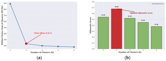
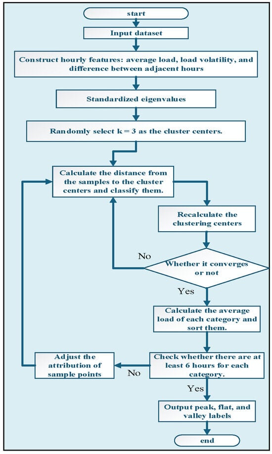
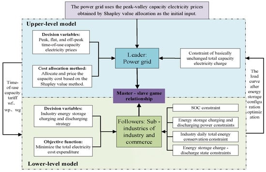
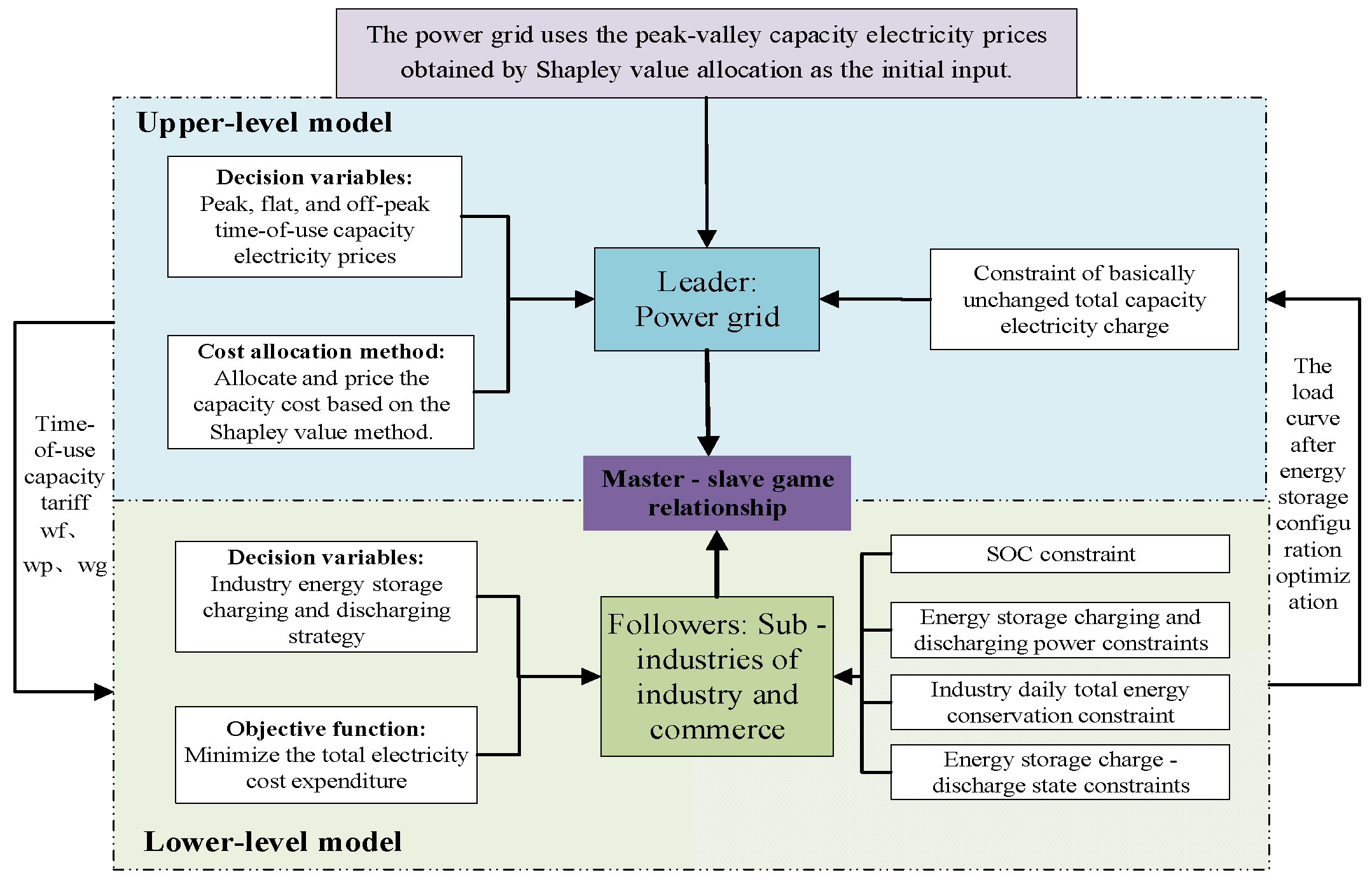
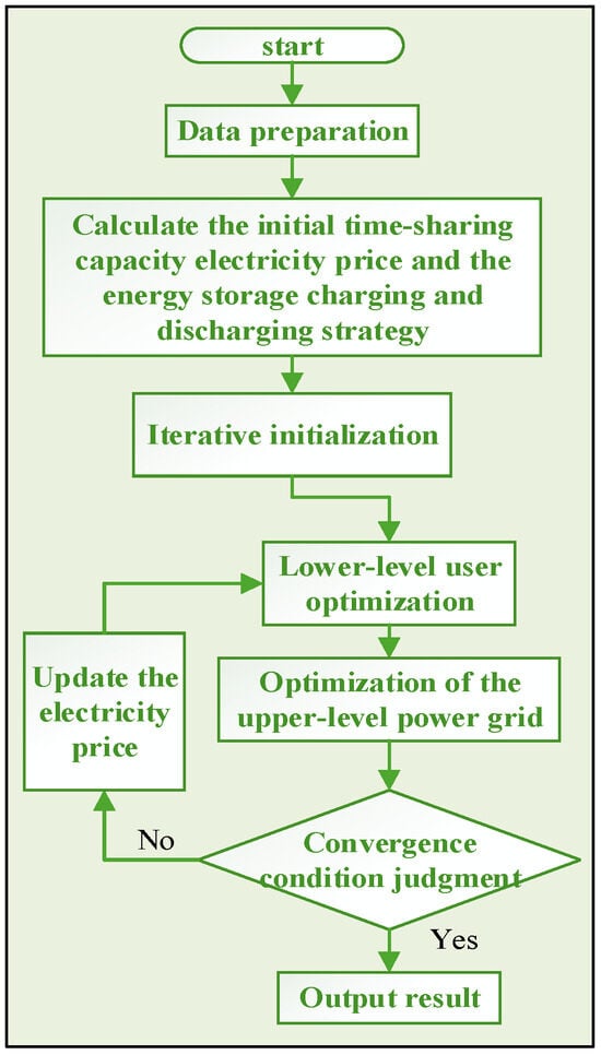
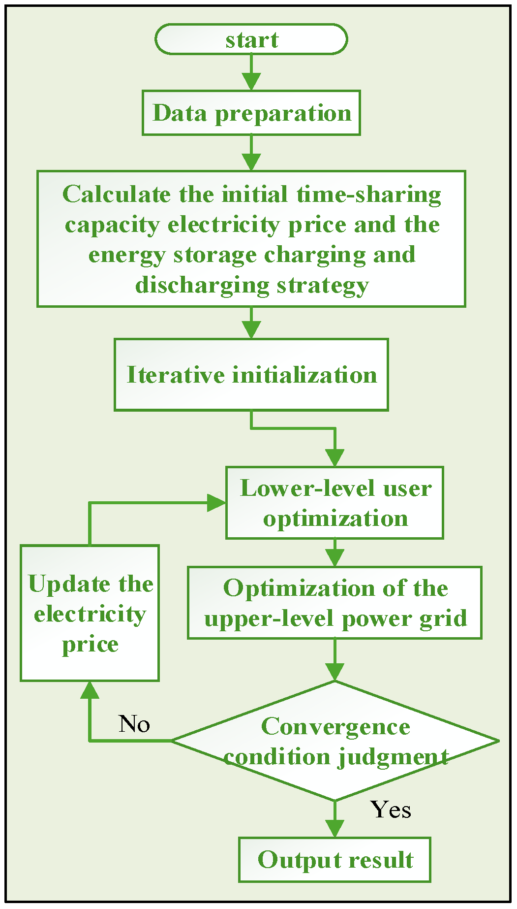
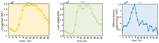
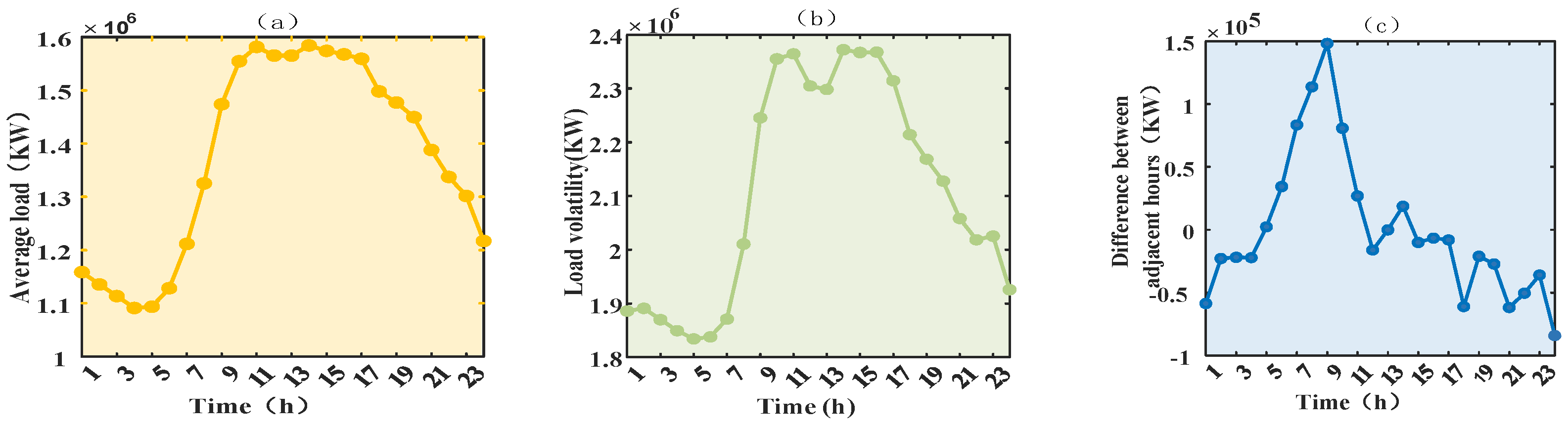
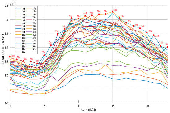
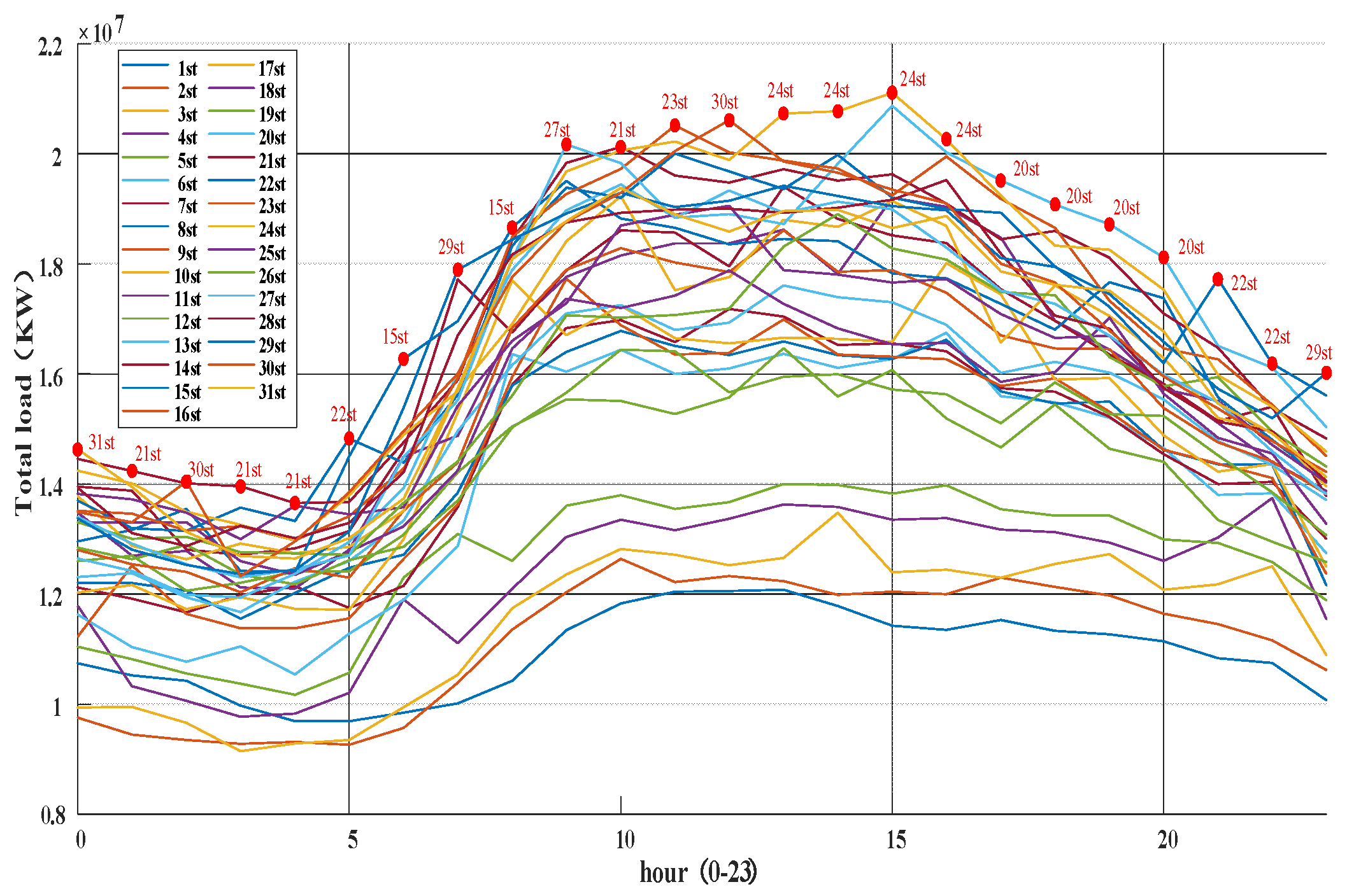
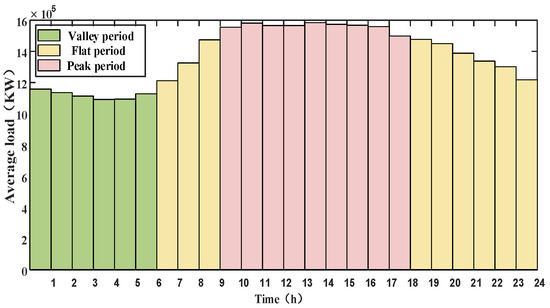
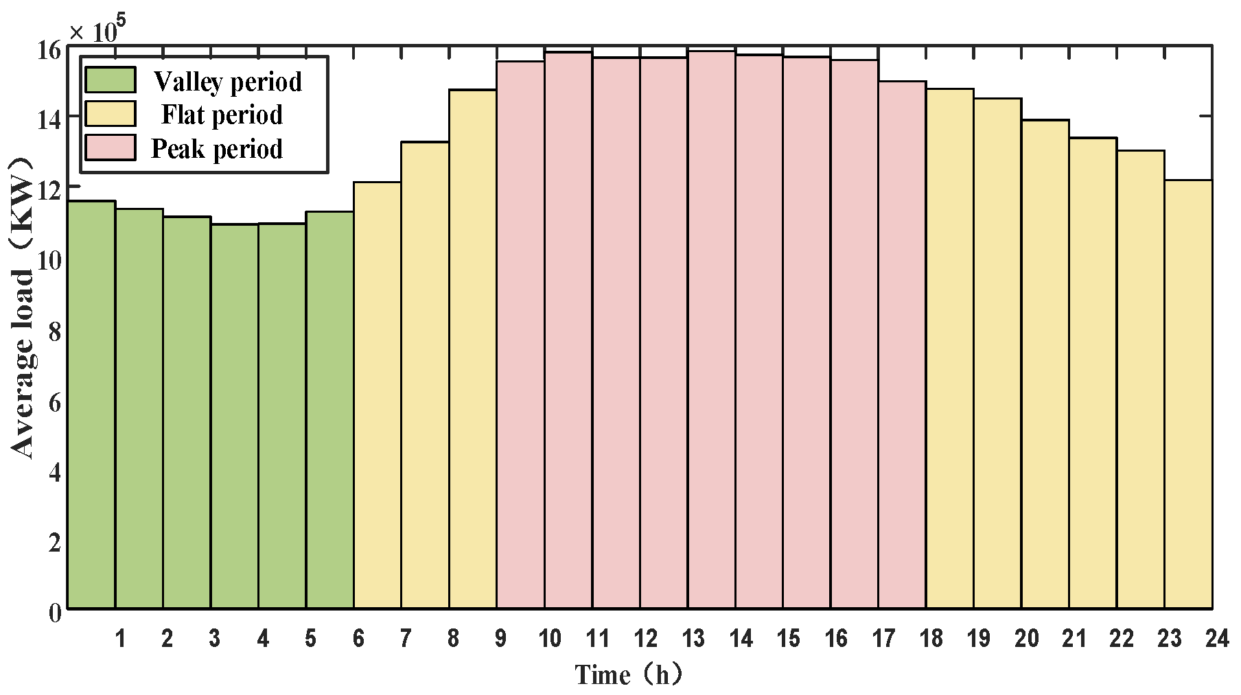
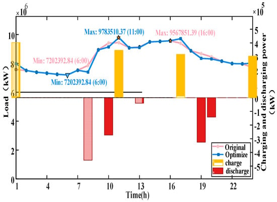
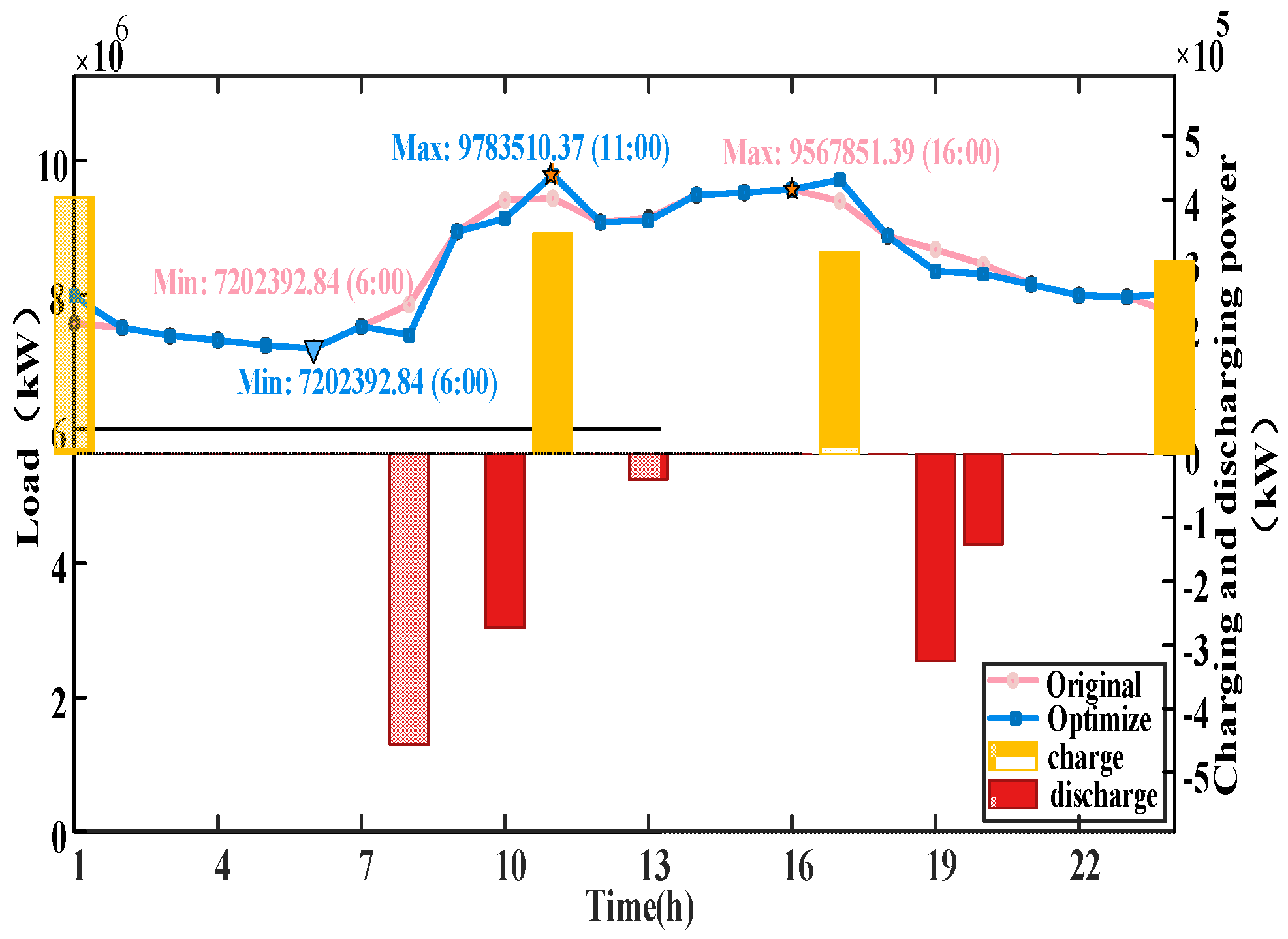
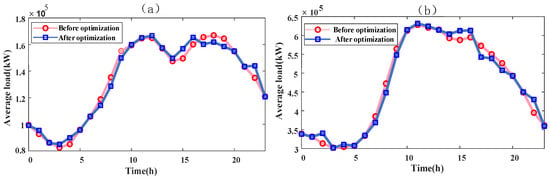
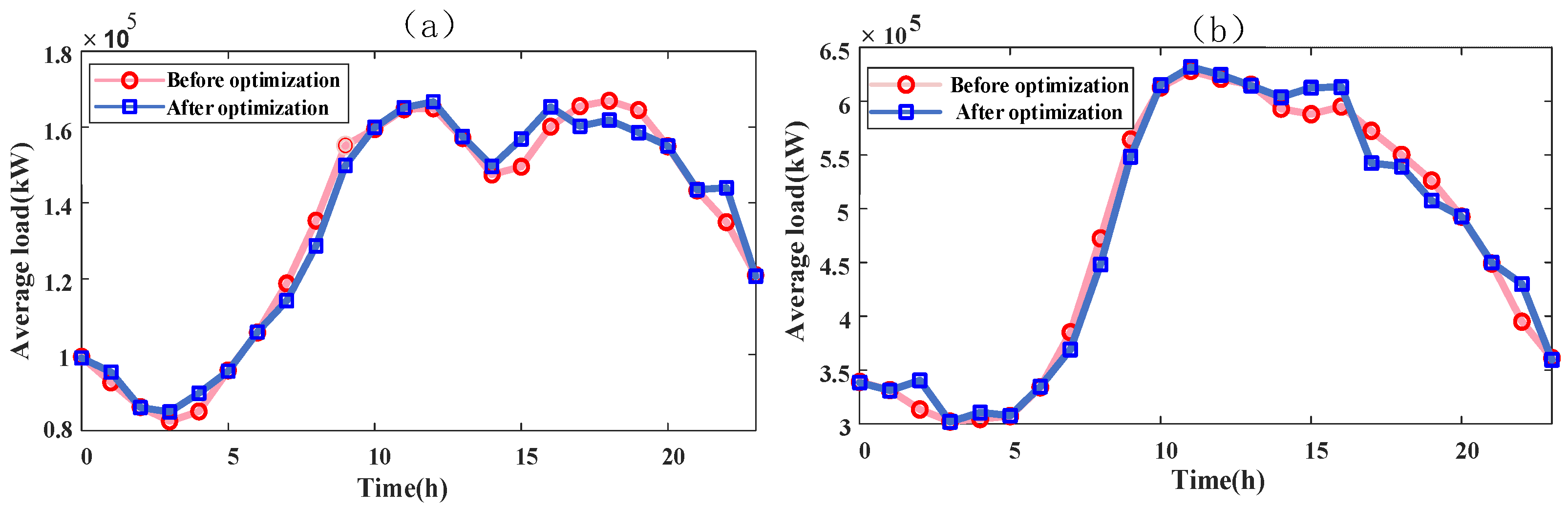

Disclaimer/Publisher’s Note: The statements, opinions and data contained in all publications are solely those of the individual author(s) and contributor(s) and not of MDPI and/or the editor(s). MDPI and/or the editor(s) disclaim responsibility for any injury to people or property resulting from any ideas, methods, instructions or products referred to in the content. |
© 2026 by the authors. Licensee MDPI, Basel, Switzerland. This article is an open access article distributed under the terms and conditions of the Creative Commons Attribution (CC BY) license.