Low-Complexity Monitoring of DC Motor Speed Sensor Additive Faults Using a Discrete Kalman Filter Observer

Abstract

This article presents an online additive fault-detection system for the speed sensor of a 200 W shunt-type direct current (DC) motor, integrated into a power module controlled by an Insulated Gate Bipolar Transistor (IGBT). The system is designed to trigger an alarm signal when an additive fault occurs by comparing the Kalman Filter (KF) residual against a predefined detection threshold. Three specific fault types in the speed sensor were analyzed: offset, disconnection, and sinusoidal noise. Experimental results demonstrate effective fault detection across a speed range of 80 to 690 rpm under no-load conditions. However, when a constant torque of 0.5 Nm is applied, both the detection threshold and the subset of reliably identifiable faults must be adjusted. The main contribution of this study is the development of a customized real-time fault detection framework and the characterization of residual variations caused by unmodeled load disturbances in actual hardware. This approach improves the monitoring and fault-diagnosis capabilities of sensor systems in DC motors by quantifying the stochastic behavior of residuals under different operating constraints.

1. Introduction

Rotating electrical machines, commonly referred to as electric motors, convert electrical energy into mechanical energy and are an essential component of modern industrial systems. Although early power systems were dominated by direct current (DC) machines, since the late 19th century, alternating current (AC) motors have gained prominence due to their robustness and ease of integration into electrical networks [1]. However, DC motors continue to be widely used in industrial and mechatronic applications due to their low inertia, high dynamic response, and ease of speed and position control, characteristics that are particularly relevant in automation, robotics, and precision motion control. In these contexts, the quality of measurements (e.g., speed) directly influences the performance of the control loop and operational reliability, making the diagnosis of sensing-related faults critical.

The increasing complexity of industrial processes responds to the need to increase the productivity, improve the product quality, reduce the operating costs, and comply with strict safety and environmental regulations [2]. Under these conditions, physical degradation mechanisms such as wear, component aging, and thermal stress induce parametric variations that can deteriorate system performance and lead to failures. If not detected in a timely manner, these failures can spread to other subsystems, shorten equipment life, cause unscheduled shutdowns, and even lead to accidents in critical applications. Consequently, early detection becomes a direct enabler of predictive maintenance and safe operation strategies, particularly when decisions are based on noisy measurements and require real-time acquisition.

Fault detection and diagnosis have been extensively studied as fundamental tools for improving the reliability and availability of dynamic systems. Classic approaches based on mathematical models allow the nominal behavior of the system to be estimated and deviations associated with faults to be detected [3]. These methods have been applied in robotic platforms [4] and unmanned aerial systems using robust observer techniques [5]. With the transition to Industry 4.0 environments, fault diagnosis is increasingly integrated into intelligent monitoring architectures and cyber–physical systems [6,7], where distributed instrumentation and sensing enable online detection schemes supported by industrial sensor networks [8]. In the specific field of electric drives, recent reviews highlight the need for reliable, interpretable, and computationally inexpensive methods that can operate under the typical constraints of embedded platforms and continuous monitoring [9].

In electric drive systems, sensor faults are particularly critical, as control strategies depend directly on the reliability of measurements. These faults are generally classified as additive faults, characterized by constant biases or offsets in the measured signals, and multiplicative faults, characterized by variations in the system’s internal parameters [10]. Additive faults can be caused by miscalibration, electrical noise, signal conditioning degradation, or partial disconnections, and usually manifest as persistent discrepancies that degrade control, increase the tracking error, and induce incorrect decisions in monitoring systems. Therefore, robust measurement noise diagnostic strategies are required that are compatible with discrete sampling and feasible for real-time implementation.

In this context, the main objective of this work is to develop a fault-detection system for the speed sensor of a direct current motor using state-observation techniques. Specifically, a discrete Kalman Filter Observer (KF) is designed for linear systems to minimize the mean-square error (MSE) of the estimate and to provide robustness against measurement noise. Based on the discrepancy between the measurement and estimation, residuals are generated to identify deviations consistent with sensing faults, while maintaining an architecture suitable for execution on platforms with limited resources.

The main scientific contributions of this work are as follows:

• Formulation and experimental implementation of a fault detection scheme for DC motor speed sensors based on a KF, aimed at systems with limited computational resources and online diagnostics.
• Obtaining a state space model from experimental identification in the linear operating region of a 200 W DC shunt motor, intended for model-based diagnostics under realistic operating conditions.
• Proposal of a method for generating and evaluating residuals using RMS analysis ($J_{RMS}$) that allows the detection of additive faults in sensors (offset, disconnection, and periodic disturbances) without requiring complex signal processing, which favors embedded implementability.
• Comprehensive experimental validation of the diagnostic scheme on an industrial platform (Lucas–Nülle), demonstrating its real-time applicability and viability for low-cost monitoring systems.
• Experimental characterization of the stochastic behavior of the KF residual under load disturbances, providing insight into how unmodeled mechanical effects influence the reliability of RMS-based fault detection metrics.

In summary, although there are various techniques for diagnosing faults in electric drives, many advanced approaches require complex models, high computational costs, or large volumes of data, which limit their implementation in industrial platforms with restricted resources and strict online operating requirements. In this context, the proposed method provides a model-based, experimentally validated, low-computational-load solution for detecting faults in speed sensing in DC motors, helping to bridge the gap between robust diagnostic techniques and their practical implementation in real-time monitoring systems.

Related Work

Sensor fault detection and isolation (SFDI) is a widely developed topic due to its direct impact on the reliability of control and monitoring systems. In electric drives, sensing faults are particularly critical because they affect both state variable estimation and controller feedback. From a modeling perspective, sensor faults are often described using additive components (bias/offsets, partial disconnections, superimposed periodic disturbances) and multiplicative components (gain or scaling errors), which allows for the design of detection schemes based on inconsistencies between measurements and models [2,3,10].

In general, diagnostic approaches can be grouped into (i) data- and learning-based methods, (ii) hybrid methods, and (iii) model-based methods. Data-based approaches have gained popularity due to their ability to capture non-linearities and complex patterns when large volumes of labelled data are available; however, their performance can degrade under changes in operating regime, unseen parametric variations, or the absence of representative faults during training, in addition to requiring computing resources and validation procedures that are not always compatible with online and embedded deployments. For these reasons, in industrial applications where interpretability, traceability, and low computational cost are required, model-based methods remain a competitive and widely used alternative [2,3].

Among model-based methods, state observers are a central strategy for SFDI, as they allow the nominal behavior of the system to be reconstructed and generate a residual (or innovation) as a fault indicator signal [11]. In this context, deterministic (e.g., Luenberger, robust observers) and stochastic observers have been proposed, among which KFs stand out for their ability to incorporate process and measurement noise statistics explicitly and to produce an innovation signal with useful properties for detection [2,3]. In particular, for discrete linear systems with Gaussian noise, the Kalman Filter innovation is a natural candidate for constructing consistent quantifiable detectors, which are highly relevant in sensor applications where measurement noise and discrete sampling are unavoidable.

A well-established line of work uses innovation (the difference between measurement and prediction) and its covariance to perform statistical tests and design thresholds with probabilistic interpretation. In this context, criteria such as NIS (Normalized Innovation Squared) or hypothesis-based tests (e.g., GLR) are used, which allow the false alarm rate to be controlled under known or estimated noise assumptions. This type of formulation is particularly attractive for real-time platforms, as the calculation of innovation and its covariance is part of the standard KF flow, avoiding additional costly signal processing steps [2,3]. Alternatively, simplified industrial implementations have also used energy metrics of the residual (e.g., RMS in sliding windows), which are easier to implement. However, they typically require careful threshold calibration and sensitivity analysis to noise and operational variations.

In electric drives, and specifically in DC motors, fault diagnosis faces practical challenges associated with load variations, saturations, friction, quantization, and electromagnetic noise, which can induce non-zero noise even under nominal conditions. Therefore, recent reviews emphasize the need for methods that balance robustness, low complexity, and viability in embedded platforms, particularly for continuous monitoring and integration into Industry 4.0 architectures [6,7,9]. In this scenario, schemes based on discrete observers are appropriate when an identified model is available in the region of operation of interest, and a solution with physical traceability is sought, capable of operating within memory and computational time constraints.

Based on this literature, a specific opportunity is identified: to design an additive fault monitoring scheme for DC motor speed sensors that is (i) consistent with the stochastic Kalman Filter framework, (ii) implementable in real time with limited resources, and (iii) experimentally validated under realistic operating conditions. Consequently, this work adopts an KF as the core of the estimation and uses residuals as diagnostic signals to monitor typical additive faults (offset, disconnection, and superimposed periodic disturbances), aiming to maintain a practical balance between detection performance and implementation complexity. Despite the extensive literature on observer-based fault detection, there is little experimental evidence on how unmodeled load disturbances affect the statistical behavior of Kalman filter residuals in real DC motor systems. This work addresses this gap by experimentally analyzing the residual behavior and its impact on RMS-based detection thresholds.

The rest of the article is organized as follows. Section 2 describes the study’s general methodology. Section 3 presents the system model and the identification procedure. Section 4 details the observer design and the fault detection algorithm. Section 5 presents the main experimental results. In Section 6, the study’s results are analyzed and discussed. Finally, Section 7 and Section 8 present the conclusions and future lines of work, respectively.

2. Methodology

This study is based on design science research (DSR) [12,13], a methodology used to develop technological devices to solve engineering problems and applied in this line of research [14,15,16]. Based on this framework, an online additive fault detection system was developed and applied to the speed sensor of a 200 W shunt DC motor, integrated into a power module controlled by an Insulated Gate Bipolar Transistor (IGBT). The methodological procedure included several iterative stages: first, the expected behavior of the sensor was modeled using a KF that estimates the nominal signal and generates a $J_{RMS}$ [17]. This $J_{RMS}$ was then compared with a predefined threshold ($T_h$) to identify additive anomalies. Finally, three types of faults were analyzed: phase shift, disconnection, and sinusoidal noise, and the system’s ability to detect them under different operating conditions was evaluated. The prototype was validated over a speed range of 80 to 690 rpm with a constant torque of 0.5 Nm, and the detection efficiency for each fault type was measured as described in [18]. A custom block was also implemented in the MATLAB toolbox, allowing real-time measurement of additive faults in the speed sensor.

3. Overall System

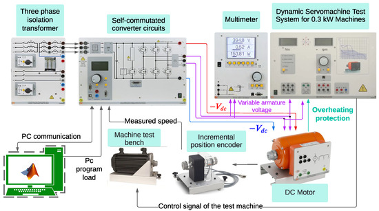
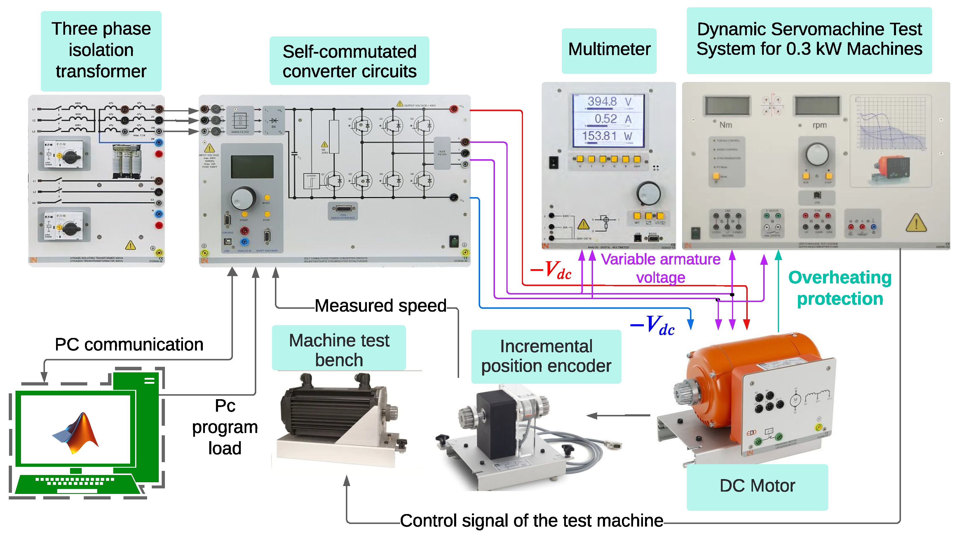
The experimental system is implemented on the Lucas Nülle (LN) modular platform, which allows the dynamic behavior of a DC motor to be evaluated under different operating and load conditions. The system’s general configuration is shown in Figure 1. The general operation of the experimental system is described below, with detailed descriptions of its main components.

Figure 1. System connection diagram.

• Power supply: Three-phase delta-star connection transformers, used to adapt, isolate, and stabilize the voltage of the electrical network that powers the experimental system.
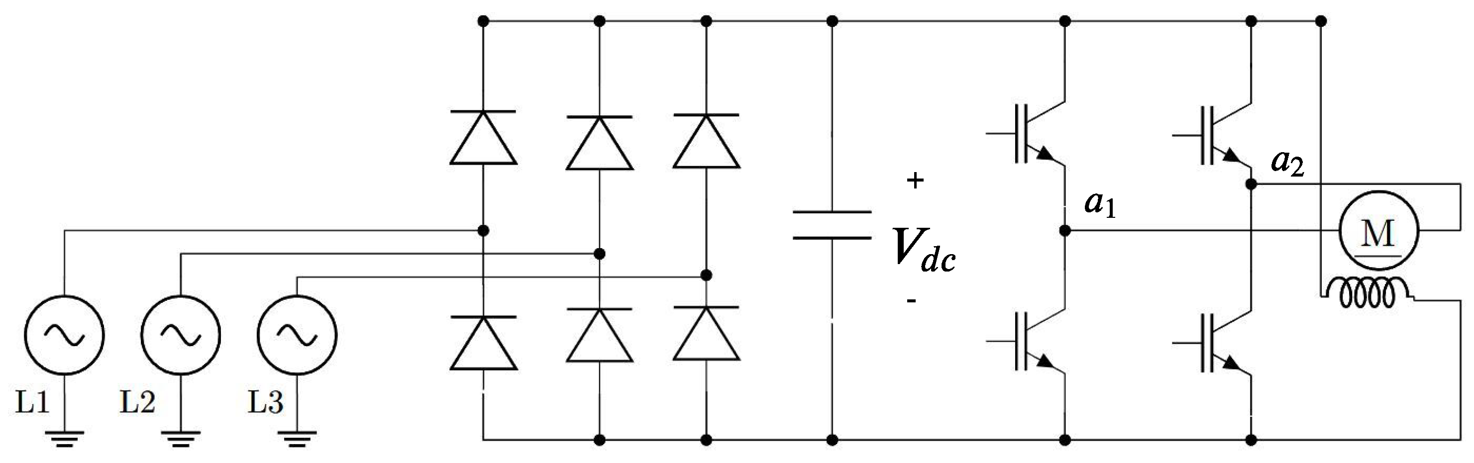
• Conversion and control: The LN CO3636-3B module integrates a switching converter based on IGBT transistors, powered by a three-phase rectifier that converts the AC input voltage to DC and a capacitor bank that stabilizes the DC bus ($V_{dc}$), reducing ripple ($\Delta V_r$) [19,20]. The voltage applied to the motor armature at terminals $a_1$ and $a_2$ is modulated to control the speed (Figure 2). During the experimental tests, the armature operating range was set to 10–70 V, while the field voltage was kept constant at $V_{dc}$ = 236 V, ensuring reproducible conditions for system modeling and identification [21,22,23].
• Test bench: LN CO3636-6V module, used to evaluate the dynamic behavior of the motor under different load conditions.
• Measurement and visualization: LN SE2663-3T incremental encoder and LN Scope toolbox, used for the acquisition and monitoring of motor speed and other relevant variables.
• Actuator: LN SE2682-3D DC motor, with a rated power of 0.2 kW, coupled to the load brake and the incremental encoder to measure speed.

Figure 2. Power supply circuit diagram for the Shunt DC Motor.

Figure 2. Power supply circuit diagram for the Shunt DC Motor.

On the other hand, the representation of a fault-free system and its analysis are divided into four parts: the system’s mathematical model, system identification, system observability, and sensor faults. Each of these is developed in Section 3.1, Section 3.2, Section 3.3 and Section 3.4, respectively. Table 1 summarizes the notations used in this article.

Table 1. General notation used in this article.

Description	Notation
System matrices	A, B, C
Fault matrix	F
Disturbance vector	V
Identity matrix	I
Observability matrix	O
Covariance matrix	$X_0$, P, M, N
Inverse matrix	$A^{-1}$
Transpose matrix	$A^T$
Gain matrix	K
Discrete time	k
Continuous time	t
Time-domain fault signal	$f\left(t\right)$
Time-domain sensor noise signal	$n\left(t\right)$
Time-domain input signal	$u\left(t\right)$
Discrete-time input signal	$u\left(k\right)$
Time-domain disturbance signal	$v\left(t\right)$
Discrete-time disturbance signal	$v\left(k\right)$
Continuous-time state vector	$x\left(t\right)$
Discrete-time state vector	$x\left(k\right)$
Discrete-time estimated state	$\widehat{x}\left(k\right)$
Continuous-time output signal	$y\left(t\right)$
Discrete-time estimated output	$\widehat{y}\left(k\right)$
Difference between the output and the estimated output	r
Expectation of a random variable	$E\{·\}$
Residual signal	$J_{\mathrm{RMS}}$
Threshold	$T_h$
Mean	${\mu }_{J_{RMS}}$
Standard deviation	${\sigma }_{J_{RMS}}$
Confidence factor	$\eta$

3.1. Mathematic Model

The state-space model defined by Equations (1) and (2) represents a linear time-invariant (LTI) system

$$\begin{array}{cc}\hfill \dot{x}\left(t\right)& =Ax\left(t\right)+Bu\left(t\right)+Vv\left(t\right),\hfill \end{array}$$

(1)

$$\begin{array}{cc}\hfill y\left(t\right)& =Cx\left(t\right),\hfill \end{array}$$

(2)

where $x\left(t\right)$ is the state vector, $u\left(t\right)$ represents the input signal, $y\left(t\right)$ corresponds to the output signal, and $v\left(t\right)$ is the disturbance vector. Matrices A, B, and C constitute the system parameters that describe the internal dynamics, input coupling, and the relationship between the state and output, respectively.

3.2. System Identification

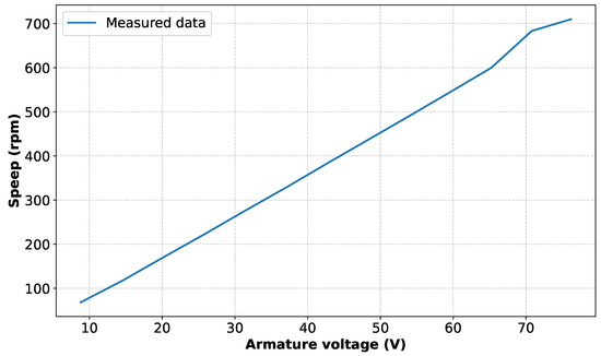
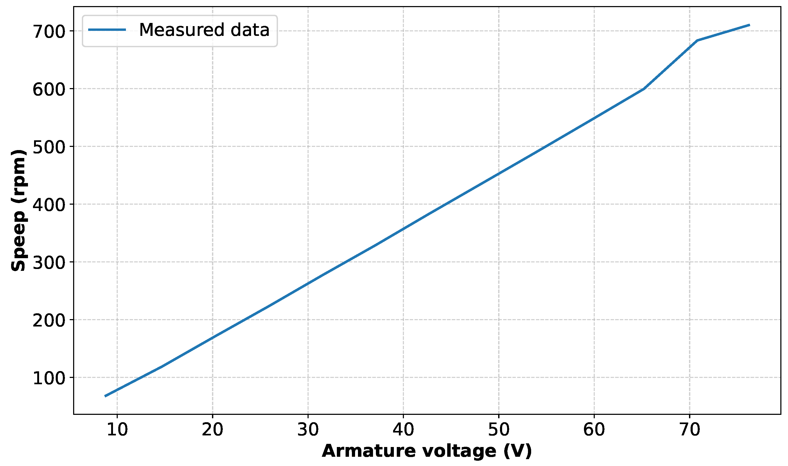
The system’s dynamic model was identified by analyzing the linear operating range from 10 V to 70 V, as shown in Figure 3.

Figure 3. Characteristic curve of the engine’s linear range.

Based on Equations (1) and (2), the system identification process was carried out using MATLAB’s System Identification Toolbox (Ident). Several model structures and parameter adjustments were evaluated to obtain the most accurate representation of the system dynamics. In addition, the perturbation matrix (V) was obtained, representing the effect of external disturbances on the system during the identification process. To ensure the reliability and generalization capability of the identified model, a cross-validation procedure was performed using independent datasets. After this validation process, the model achieved a best fit of 94.89%. Based on this result, the state-space matrices A, B, and C in Equations (1) and (2) were determined, leading to the state-space representation given in Equations (3) and (4), with the inclusion of V accounting for perturbations in the system.

$$\begin{array}{c}\hfill \left[\begin{array}{c}{\dot{x}}_1\left(t\right)\\ {\dot{x}}_2\left(t\right)\end{array}\right]=\left[\begin{array}{cc}0& 1\\ -1980.5772& -77.9790\end{array}\right]\left[\begin{array}{c}{x}_1\left(t\right)\\ x_2\left(t\right)\end{array}\right]+\left[\begin{array}{c}0\\ -20879.13\end{array}\right]u\left(t\right)+\left[\begin{array}{c}448.0265\\ 6263.0274\end{array}\right]v\left(t\right)\end{array}$$

(3)

$$\begin{array}{c}\hfill y\left(t\right)=\left[\begin{array}{cc}1& 0\end{array}\right]\left[\begin{array}{c}{x}_1\left(t\right)\\ x_2\left(t\right)\end{array}\right]\end{array}$$

(4)

On the other hand, the matrix resulting from the eigenvalues of $|sI-A|$ is determined by Equation (5), which confirms that the eigenvalues are in the left half-plane of the complex plane and indicates that the system is stable.

$$\begin{array}{c}\hfill |sI-A|=\left[\begin{array}{c}-38.9895+21.4568i\\ -38.9895-21.4568i\end{array}\right]\end{array}$$

(5)

3.3. System Observability

The LTI system is considered observable if and only if the initial state $x\left(t_0\right)$ can be determined from knowledge of the input $u\left(t\right)$, the output $y\left(t\right)$, and the system matrices A, B, and C in a finite time interval $t_0\le t\le t_f$. In summary, the observability property guarantees that, for some finite value $t_f$, each internal state of the system can be inferred from the output measurements [24]. Equation (6) defines the observability matrix O of the system.

$$\begin{array}{c}\hfill O=\left[\begin{array}{c}C\\ C{A}^2\\ ⋮\\ C{A}^{n-1}\end{array}\right]\end{array}$$

(6)

The observability property of the system is evaluated by analyzing the pair of matrices [$A,C$]. A system is completely observable if and only if the observability matrix O has full rank ($\mathrm{rank}\left(O\right)=n$, where n is the order of the system). Based on A, C and Equations (3) and (4), we obtain $\mathrm{rank}\left(O\right)$. Since $\mathrm{rank}\left(O\right)=2$, we confirm that the system is fully observable.

$$\begin{array}{c}\hfill \mathrm{rank}\left(O\right)=\mathrm{rank}\left(\left[\begin{array}{c}C\\ CA\end{array}\right]\right)=\mathrm{rank}\left(\left[\begin{array}{cc}1& 0\\ 0& 1\end{array}\right]\right)=2\end{array}$$

(7)

3.4. Sensors Failures

Sensor faults are caused by factors such as incorrect calibration, noise coupling, disconnection, and scaling errors. Therefore, based on Equations (1) and (2), sensor faults are modeled using Equations (8) and (9), considering the factors as additive.

$$\begin{array}{cc}\hfill \dot{x}& =Ax\left(t\right)+Bu\left(t\right)+Vv\left(t\right)\hfill \end{array}$$

(8)

$$\begin{array}{cc}\hfill y\left(t\right)& =Cx\left(t\right)+Ff\left(t\right)+n\left(t\right),\hfill \end{array}$$

(9)

where $n\left(t\right)$ is the sensor noise signal and F is the fault matrix. Decalibration faults are deviations from the actual measurement and can be positive or negative. Other faults include sinusoidal noise, which represents encoder wear and can cause oscillations in its measurements. The frequency set in the analysis is based on [25]. Finally, disconnection is represented as a value of 0 in the sensor. Table 2 shows the values of the additive faults of the sensor.

Table 2. Additional sensor faults.

Failures Type	Value (rpm)
Off set	10
Disconnection	0
Sinusoidal noise	$10·sin$

4. The Proposed KF Design

This section presents the KF design, the $J_{RMS}$ evaluation, and the development of the fault detection algorithm.

4.1. KF Design

The discrete-time KF is affected by stochastic noise in the input $v\left(k\right)$ and output $n\left(k\right)$ [26,27]. In continuous time, $v\left(t\right)$ represents physical forces such as the load torque; the discrete-time term $v\left(k\right)$ captures the integrated effect of these disturbances over the sampling interval $T_s$. This approach allows the model to account for discretization errors and unmodeled mechanical dynamics that are not explicitly defined in the state equations. It is based on a state-space model defined by Equations (10) and (11), assuming a linear time-invariant process.

$$\begin{array}{cc}\hfill x(k+1)& =Ax\left(k\right)+Bu\left(k\right)+Vv\left(k\right)\hfill \end{array}$$

(10)

$$\begin{array}{cc}\hfill y\left(k\right)& =Cx\left(k\right)+n\left(k\right)\hfill \end{array}$$

(11)

The matrices A, B, C, and V are known from the identified system. Although the initial state is unknown, the probabilistic information about $x\left(0\right)$, $v\left(k\right)$, and $n\left(k\right)$ is known. It is assumed that these stochastic variables are statistically independent and are Gaussian distributed, with mean values defined by $E\left\{x\right(0\left)\right\}$, $E\left\{v\right(k\left)\right\}$, and $E\left\{n\right(k\left)\right\}$.

$$\begin{array}{c}\hfill E\left\{x\left(0\right)\right\}=x_0;E\left\{v\left(k\right)\right\}=0;E\left\{n\left(k\right)\right\}=0\end{array}$$

(12)

On the other hand, Equations (13)–(15) define the covariance matrices $X_0$, M and N

$$\begin{array}{cc}\hfill X_0& =E\left\{(x\left(0\right)-x_0){(x\left(0\right)-x-0)}^T\right\}\hfill \end{array}$$

(13)

$$\begin{array}{cc}\hfill M& =E\left\{v\left(k\right)v^T\left(k\right)\right\}\hfill \end{array}$$

(14)

$$\begin{array}{cc}\hfill N& =E\left\{n\left(k\right)n^T\left(k\right)\right\},\hfill \end{array}$$

(15)

where M and N are known to provide a measure of the noise size. Likewise, KF is divided into two parts: the prediction defined by Equations (16) and (17) and the correction defined by Equations (18)–(20):

$$\begin{array}{cc}\hfill & \widehat{x}(k+1|k)=A\widehat{x}\left(k\right|k)+Bu\left(k\right)\hfill \end{array}$$

(16)

$$\begin{array}{cc}\hfill & P^{-}(k+1)=AP\left(k\right)A^T+VM{V}^T\hfill \end{array}$$

(17)

$$\begin{array}{cc}\hfill K(k+1)& =P^{-}(k+1)C^T{[C{P}^{-}(k+1)C^T+N]}^{-1}\hfill \end{array}$$

(18)

$$\begin{array}{cc}\hfill \widehat{x}(k+1|k+1)& =\widehat{x}(k+1|k)+\widehat{K}[y(k+1)-C\widehat{x}(k+1|k)]\hfill \end{array}$$

(19)

$$\begin{array}{cc}\hfill P(k+1)& =[I-K(k+1)C]P^{-}(k+1),\hfill \end{array}$$

(20)

where P is the covariance matrix, I is the identity matrix, and K is the correction matrix. Based on Equations (16)–(20), the recursive estimate $\widehat{x}(k+1|k+1)$ of KF defined in Equation (21) is obtained.

$$\begin{array}{c}\hfill \widehat{x}(k+1|k+1)=A\widehat{x}\left(k\right|k)+Bu\left(k\right)+K(k+1)[y(k+1)-C(A\widehat{x}\left(k\right|k)+Bu\left(k\right))]\end{array}$$

(21)

4.2. Residual Evaluation

The evaluation of $J_{RMS}$ based on the root mean square (RMS) value is defined in Equation (22), while the configuration $T_h$ is established by Equation (23). $J_{RMS}$ measures the average energy of the residual in the interval $(k+N)$. Likewise, $T_h$ allows the tolerance limit to be determined in relation to model uncertainties under fault-free operating conditions. In this way, fault detection is effective by comparing the evaluation of $J_{RMS}$ and $T_h$:

$$\begin{array}{c}\hfill J_{RMS}={\parallel r\left(k\right)\parallel }_{RMS}=\sqrt{{\displaystyle \frac{1}{N}}\sum _{j=1}^N{\parallel r(k+j)\parallel }^2},\end{array}$$

(22)

$$T_h={\mu }_{J_{RMS}}+\eta {\sigma }_{J_{RMS}},$$

(23)

where ${\mu }_{J_{RMS}}$ is the mean of the $J_{RMS}$, ${\sigma }_{J_{RMS}}$ is the standard deviation, and $\eta =2$ is the confidence factor. The value of $T_h$ was obtained through statistical analysis of the RMS of the residuals under fault-free conditions, considering the variability associated with model uncertainties and measurement noise. The final value selected ensures an adequate compromise between false alarm reduction and fault detection sensitivity. The statistical parameters ${\mu }_{J_{RMS}}$ and ${\sigma }_{J_{RMS}}$ were estimated from experimental data collected under nominal operating conditions, allowing the threshold to represent the natural stochastic variability of the residual in fault-free operation.

The detection logic is defined by a decision rule that uses the established threshold. In particular, when $J_{RMS}>T_h$, the fault is detected. Conversely, if $J_{RMS}\le T_h$, the system operates in a fault-free condition.

Furthermore, it should be noted that the residual evaluation metric was intentionally designed to be computationally light. The proposed fault detection strategy is intended to be implemented in an embedded controller performing fluid control tasks, with only approximately 80 kB of memory allocated specifically to the diagnostic module. This memory limitation restricts the use of computationally more demanding statistical detection tests, such as the normalized innovation squared (NIS) or the generalized likelihood ratio (GLR). For this reason, the RMS-based residual metric was selected as a practical compromise, enabling real-time execution with low computational and memory requirements while providing reliable fault detection performance for operating conditions that remain reasonably close to the identified operating point.

4.3. Fault Detection Algorithm

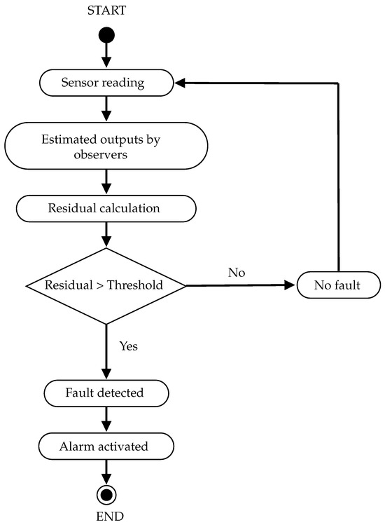
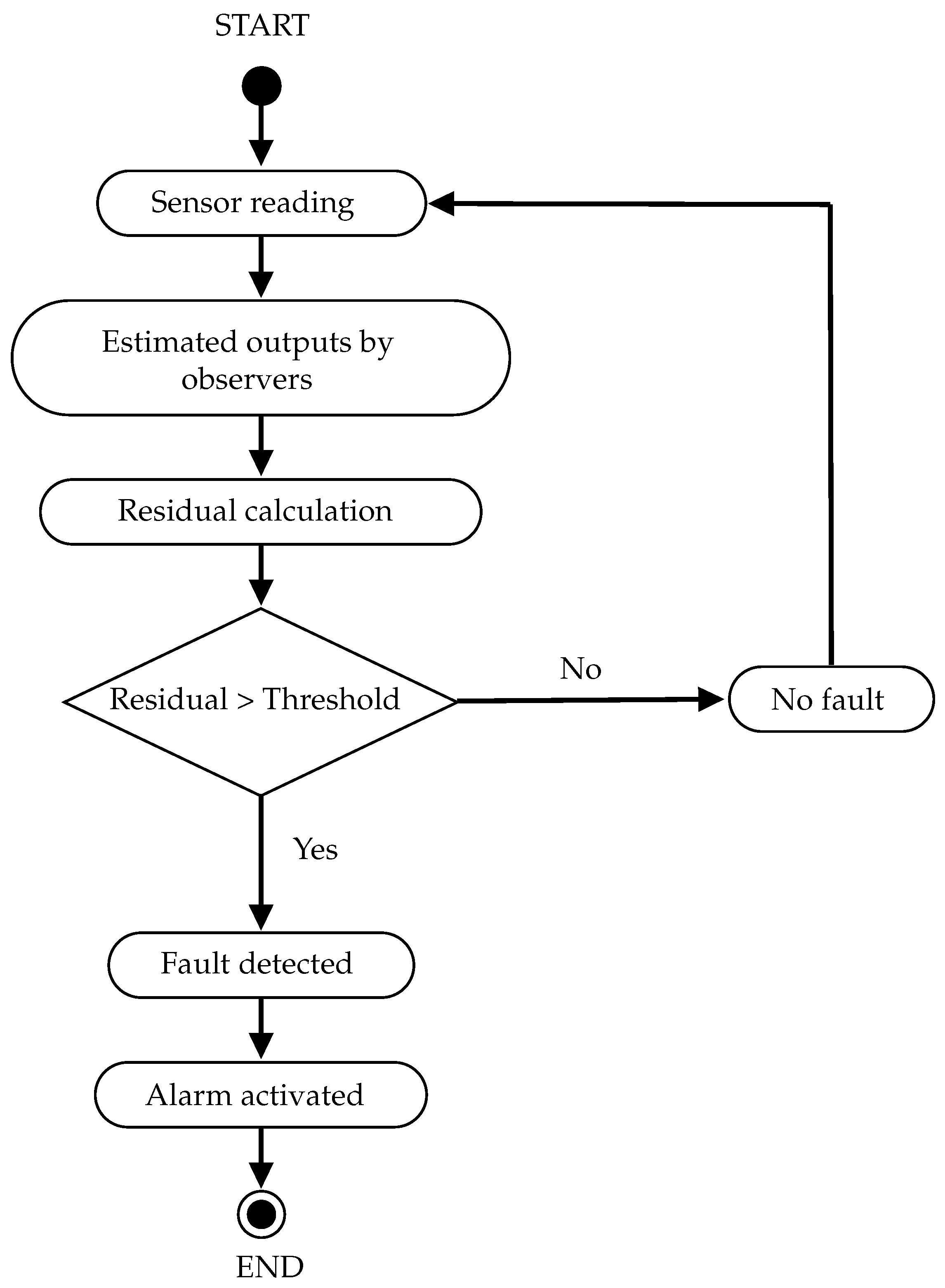
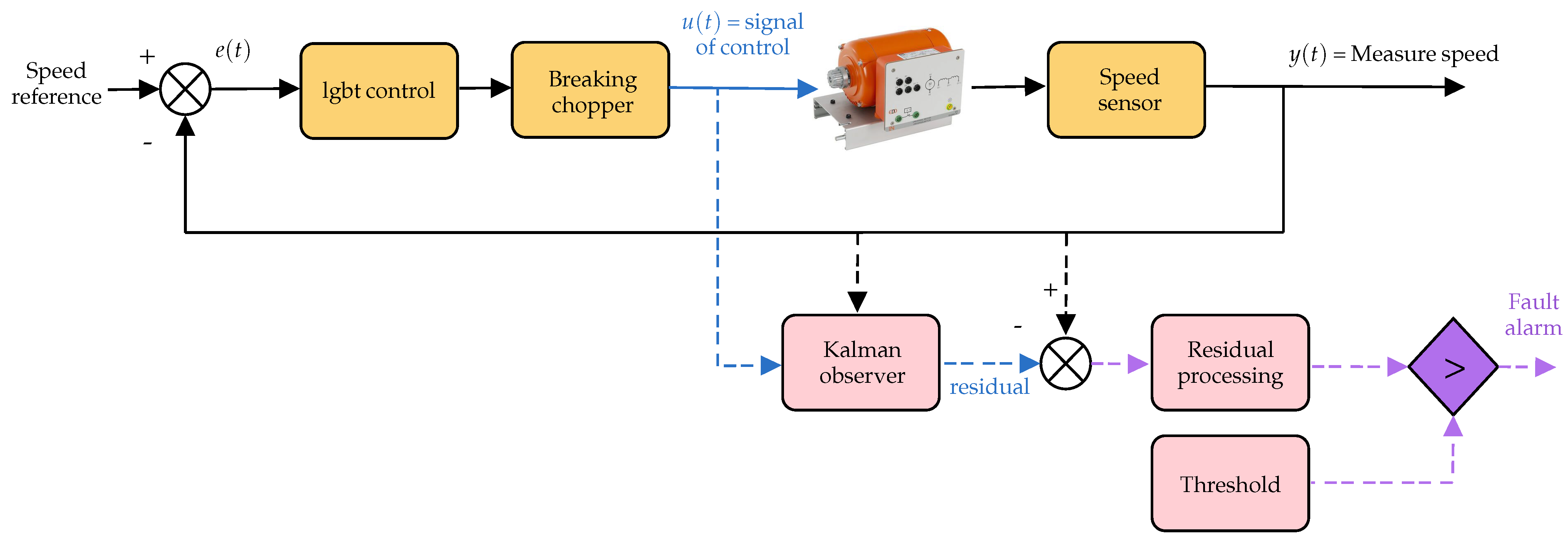
Figure 4 shows the logical sequence of the fault detection process. It begins with the acquisition of the input variables $y\left(t\right)$ and $u\left(t\right)$. Then, the KF estimates the motor speed $\widehat{y}\left(t\right)$. Furthermore, the difference between $y\left(t\right)$ and $\widehat{y}\left(t\right)$ generates the estimation error, whose magnitude is evaluated using an RMS over a 5-sample window, allowing for rapid detection at low computational cost. If this value exceeds a predefined threshold calculated using Equations (22) and (23), the system activates a fault alarm; otherwise, the process continues in normal operation. This approach allows anomalies to be detected in advance without compromising system stability.

Figure 4. General block diagram of the system implemented in MATLAB/Simulink.

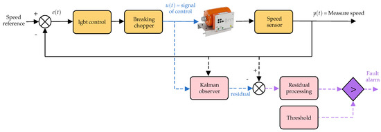
Figure 5 shows the general block diagram of the system implemented in MATLAB/Simulink R2023b. It also shows the interaction between the main control loop, the braking chopper, the speed feedback, and the fault detection subsystem. The latter integrates the KF, the calculation of $J_{RMS}$, and the logic for activating the alarm.

Figure 5. Block diagram of the fault detection system.

The KF block uses a discrete representation of the system. For its implementation, the values of A, B, C, and V obtained from Equations (3) and (4) in their discrete representation were used. The matrices were discretized with a sampling time of $T_s=0.000125$ s. This value was selected to ensure consistency with the IGBT module’s 8 kHz operating frequency, thereby guaranteeing the temporal synchrony of operations. Based on this procedure, new values of A, B, C and V are obtained in Equation (24).

$$\begin{array}{c}\hfill A=\left[\begin{array}{cc}1& 0.0001\\ -0.2464& 0.9903\end{array}\right],B=\left[\begin{array}{c}-0.0035\\ 2.5976\end{array}\right],V=\left[\begin{array}{c}0.0561\\ 0.7722\end{array}\right]\end{array}$$

(24)

Based on Equations (14) and (15), we obtain $M=0.1$ and $N=0.01$ (found from the system identification). At the same time, the gain (K) is calculated using Equation (18), taking the initial value of the matrix P defined in Equation (25).

$$\begin{array}{c}\hfill P=\left[\begin{array}{cc}0.001& 0\\ 0& 0.001\end{array}\right]\end{array}$$

(25)

Algorithm 1 presents the implementation of the proposed KF, incorporating the discretized model matrices, along with the prediction, gain calculation, state update, and estimated output stages.

Algorithm 1 Discrete Kalman Filter State Estimation

Require:

System Matrices: $A,B,C,V,M$ y N.          ▹ See Equation (24)

Initialize the estimated state vector: $\widehat{x}\left(0\right)=\left|\begin{array}{c}0\\ 0\end{array}\right|$.

Initialize the error covariance matrix: $P\left(0\right)$.      ▹ See Equation (25)

Ensure: Estimated state vector $\widehat{x}$ and estimated output value $\widehat{y}$.

State Prediction: Compute $\widehat{x}=A\widehat{x}+Bu$.

Covariance Prediction: Compute $P=AP{A}^{\prime }+VM{V}^{\prime }$.

Kalman Gain: Compute the gain matrix $K=P{C}^{\prime }{(CP{C}^{\prime }+N)}^{-1}$.

State Update: Compute $\widehat{x}=\widehat{x}+K(y-C\widehat{x})$.

Covariance Update: Compute $P=(I-KC)P$.

Output Estimation: $\widehat{y}=C\widehat{x}$.

5. Results

This section presents the main results obtained from the proposed models. The fault detection system is validated through numerical simulations and experimental tests. Initially, the accuracy of the implemented model is verified; subsequently, different fault occurrence scenarios are analyzed to evaluate the performance of the proposed method.

The experimental results are organized into two operating conditions. First, the behavior of the detection system under normal operating conditions (without faults) is analyzed. Next, the results obtained when the system operates in the presence of faults are presented. In both cases, the correct functioning of the detection system is evaluated and validated experimentally. Finally, a comparison is made between the results obtained under normal and fault conditions, identifying the main differences observed.

The hardware used for the experimental development consisted of the CO3636-3B module, a self-switched power electronics training system based on IGBT devices. The hardware also integrates a control and measurement unit based on a digital signal processor (DSP), which acquires variables such as speed and voltage and provides electronic protection against overvoltage and overload. The acquisition and analysis of the experimental data were carried out using blocks connected to the hardware, enabling the real-time monitoring and systematic recording of the electrical variables. Likewise, the MATLAB interface facilitated the implementation and experimental validation of the fault detection algorithms on real hardware.

5.1. Experimental Setup and Implementation

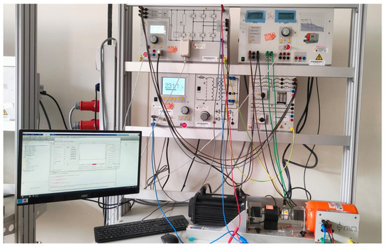
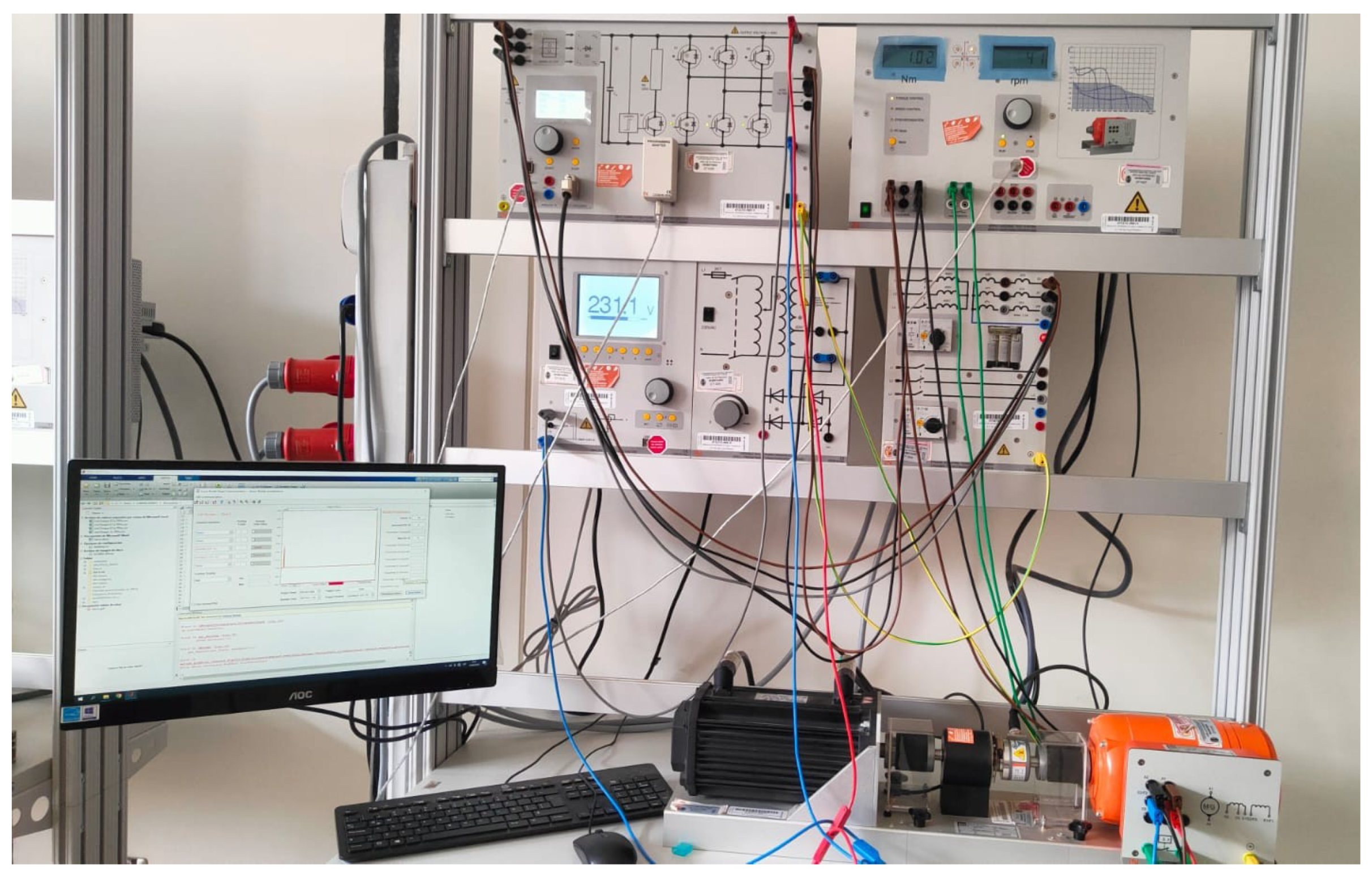
Figure 6 shows the physical implementation of the proposed fault detection system on the LN modular platform. The configuration comprises the power supply stage, the CO3636-3B converter, the CO3636-6V test bench, the SE2682-3D DC motor, and the SE2663-3T encoder integrated with the LN Scope toolbox for data acquisition and monitoring. This experimental configuration was used to validate the proposed method under different operating and load conditions.

Figure 6. Experimental setup of the proposed fault detection system implemented on the LN modular platform.

5.2. Experimental Validation Without Failure

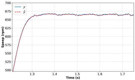
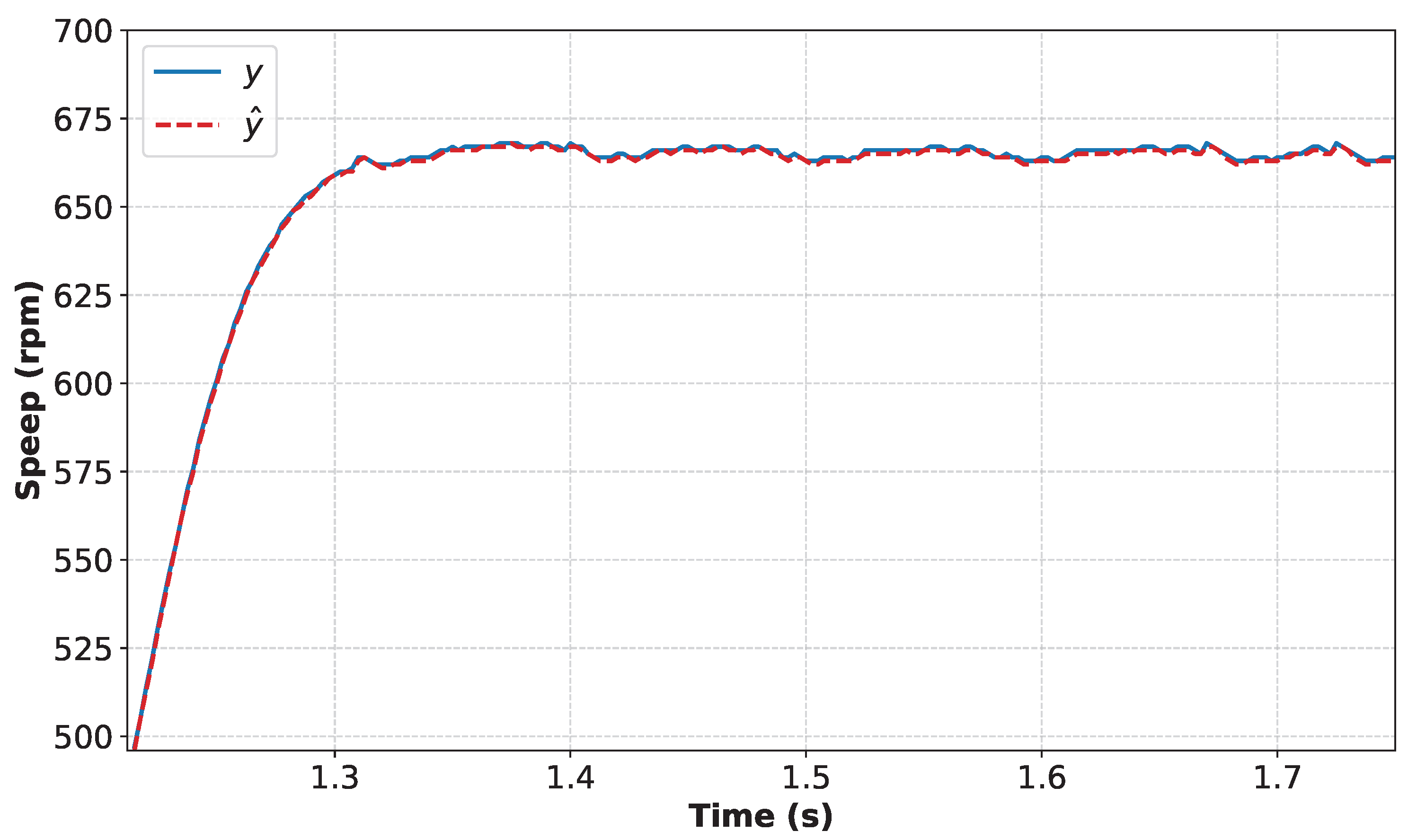
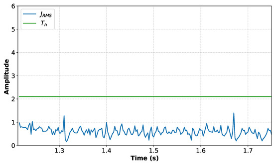
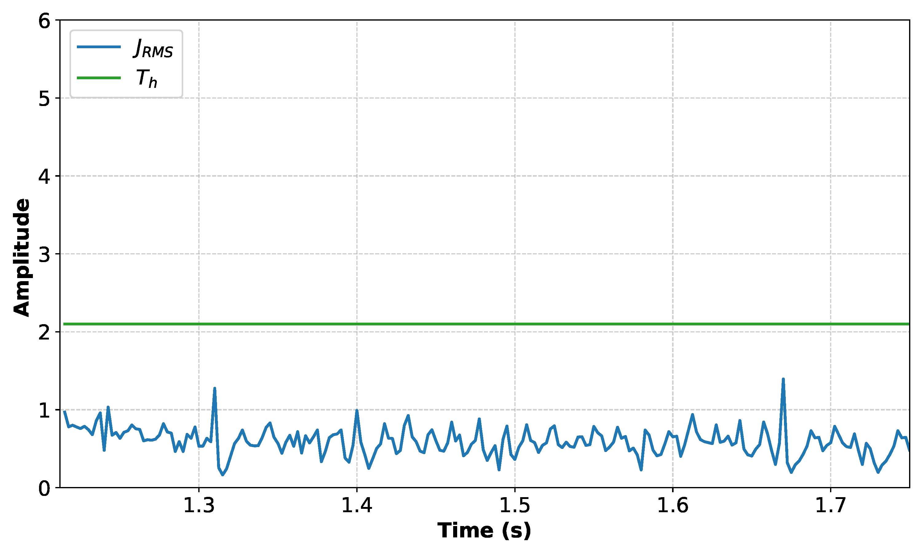
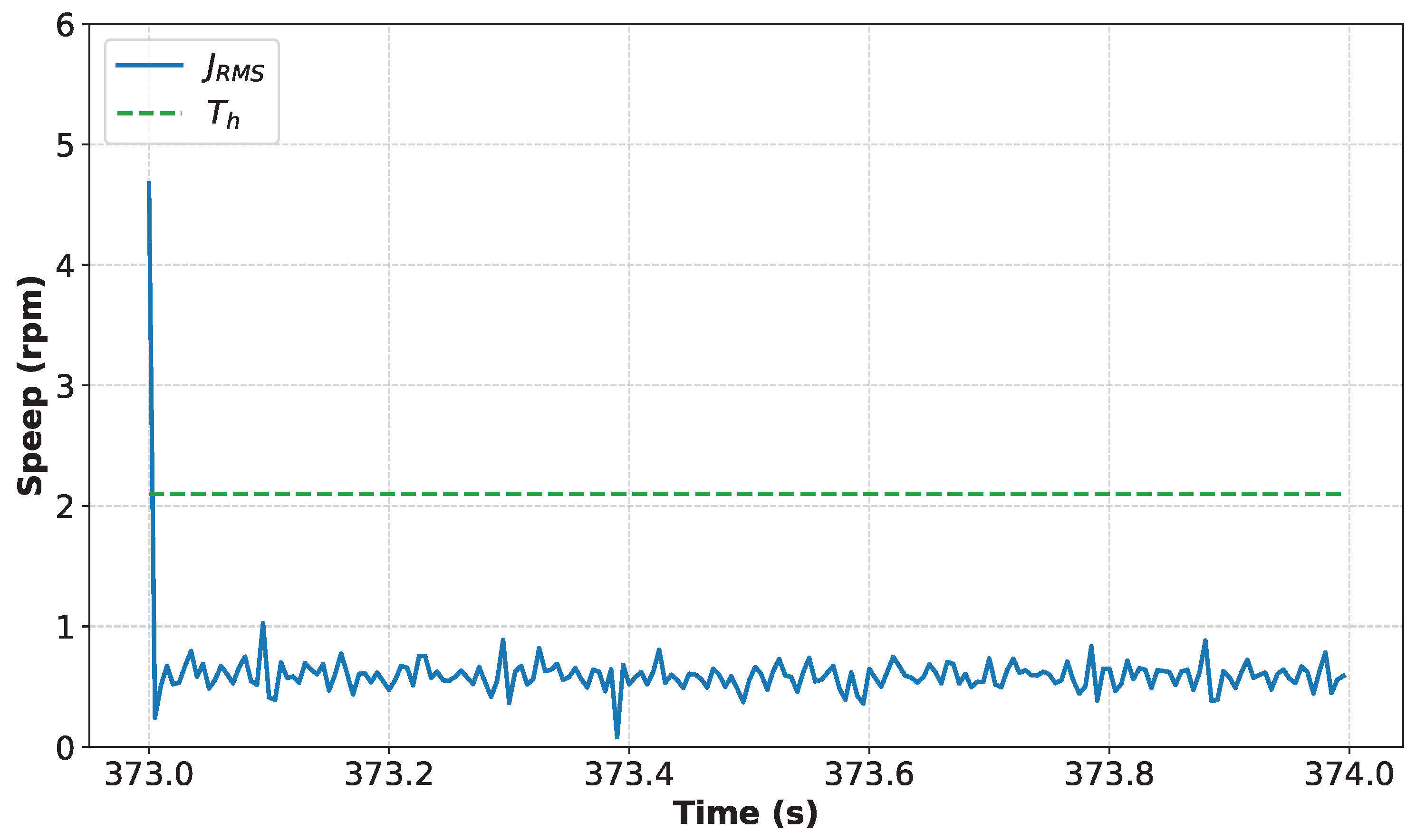
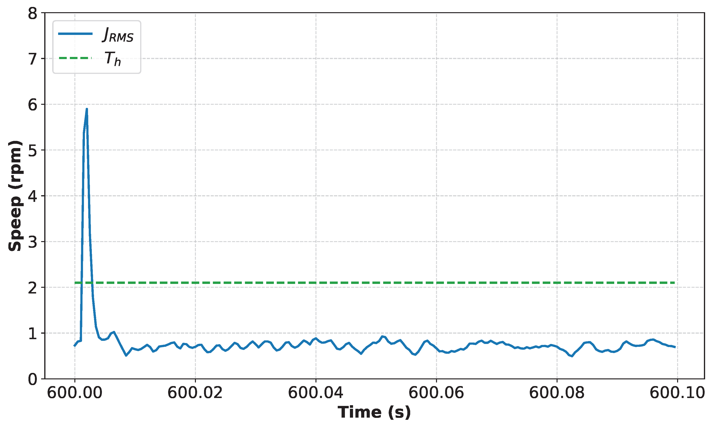
Figure 7 shows the estimated fault-free speed of the KF performance. It can be seen that the measured output speed y and the estimated output speed $\widehat{y}$ exhibit the same behavior as the time increases and in response to variations in the voltage applied to the motor armature. Figure 8 shows $J_{RMS}$ and $T_h$ as a function of time. $J_{RMS}$ has significant peaks, while $T_h$ is constant, as it was set to 2.1 after testing within the operating range of the system (10–70 V on the armature) based on Equation (23). The KF has a high estimation accuracy. Despite an MSE of 0.64, the corresponding RMSE is less than 0.2 % of the nominal speed, confirming the effectiveness of the KF in tracking the system dynamics.

Figure 7. System response in the absence of faults.

Figure 8. $J_{RMS}$ of the fault-free system.

5.3. Experimental Validation with Faults

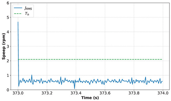
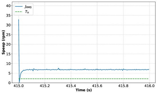
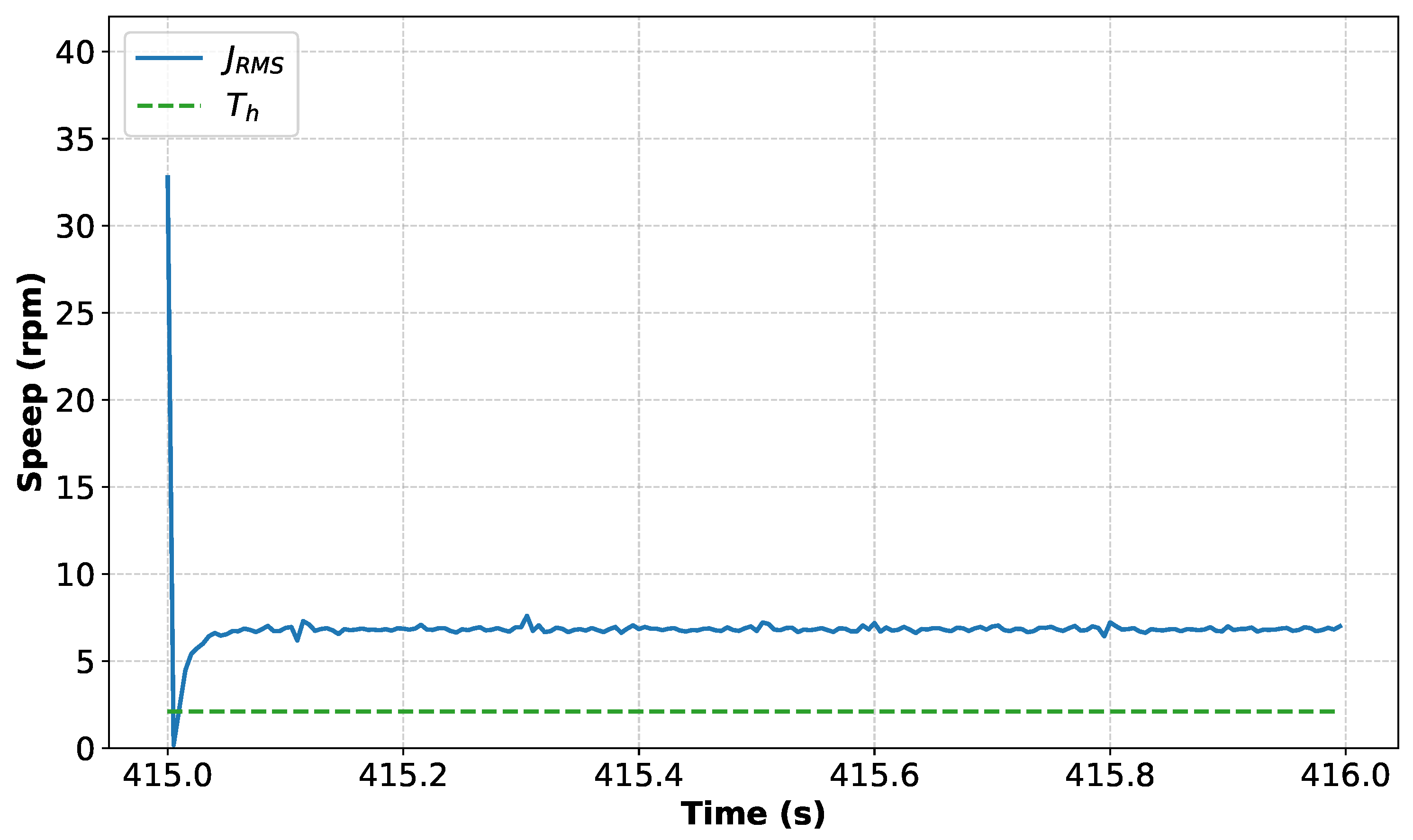
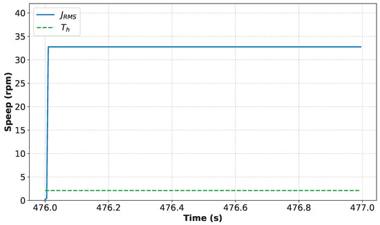
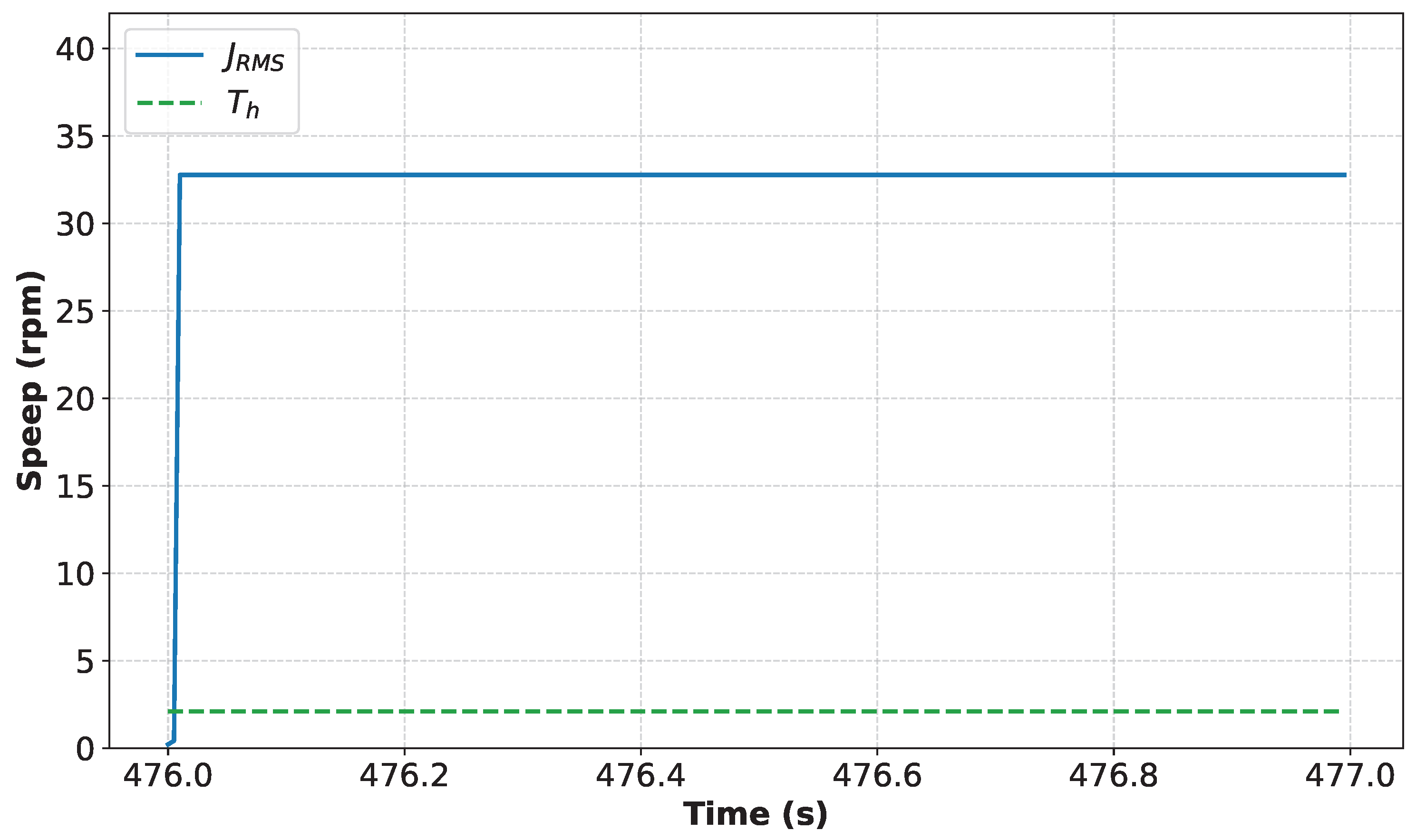
Figure 9 shows the behavior of $J_{RMS}$ in the event of an offset fault. In this case, a disturbance of +10 rpm was injected into the sensor signal, and a detection $T_h$ of 2.1 rpm was established. Under conditions without applied torque, $J_{RMS}$ exceeds $T_h$, confirming satisfactory detection. However, when applying a constant torque of 0.5 Nm to the rotor, false alarms were observed, as the observer was unable to consistently detect an offset of 10 rpm, requiring an amplitude of 20 rpm or more for reliable detection. For this reason, the detection $T_h$ was increased to ensure the identification of offset faults in the presence of torque. Figure 10 shows the behavior of $J_{RMS}$ in the event of a disconnection-type fault. In this case, the sensor signal was abruptly reduced to simulate a partial loss of measurement. In the absence of torque, the $J_{RMS}$ exceeded the $T_h$ of 2.1 rpm, achieving successful detection. However, when torque was applied to the system, false alarms were recorded; so, the threshold was adjusted to maintain the detection scheme’s reliable performance. Figure 11 shows the response of $J_{RMS}$ to a sinusoidal noise-type fault, generated by adding >$10sin\left(2\pi 60t\right)$ rpm to the sensor signal. In this case, the $J_{RMS}$ also exceeded the $T_h$ of 2.1 rpm, indicating correct detection under no-torque conditions.

Figure 9. $J_{RMS}$ for offset type fault.

Figure 10. $J_{RMS}$ for disconnection type fault.

Figure 11. $J_{RMS}$ for sinusoidal fault.

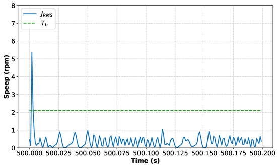
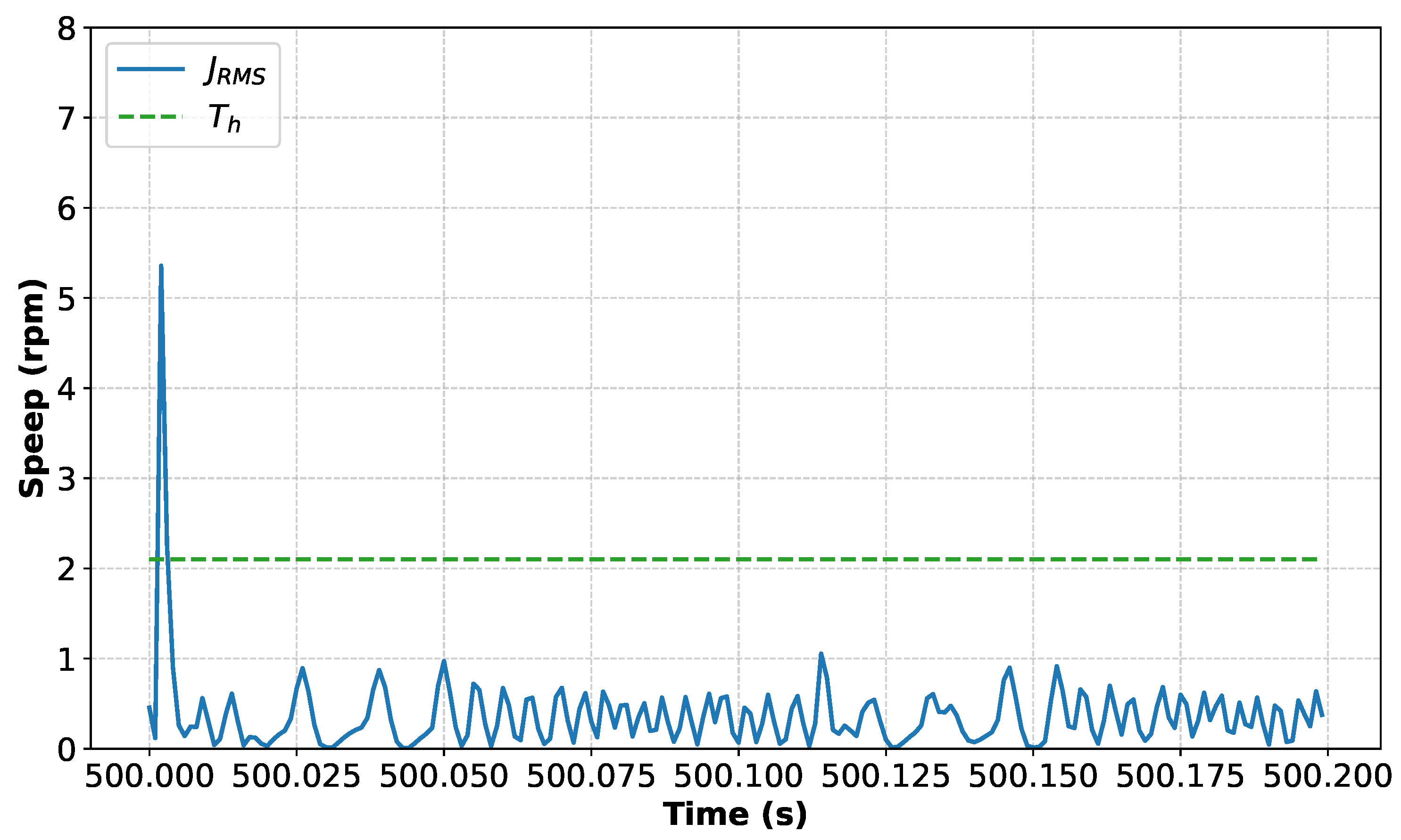
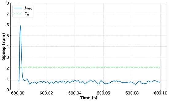
Finally, Figure 12 and Figure 13 show the system response when a torque is applied in the presence of additive faults with amplitudes of 10 and 20, respectively. In both cases, the proposed method achieves correct fault detection, as indicated by the $J_{RMS}$ index exceeding the detection threshold.

Figure 12. $J_{RMS}$ for offset type fault with 0.2 Nm.

Figure 13. $J_{RMS}$ for offset type fault with 0.5 Nm.

Table 3 summarizes the fault detection performance under different perturbations in the speed signal for operating conditions without and with applied torque, respectively. The results indicate that lower values of the threshold $T_h$ increase the detection sensitivity under torque-free conditions, resulting in shorter detection times. To provide a clearer quantitative evaluation, the absolute values of the False Alarm Rate (FAR) are reported under both no-load and load conditions. Table 4 summarizes these metrics for the different operating points. Under no-load conditions, the FAR is 0%, indicating that the fixed threshold $T_h$ remains robust under nominal conditions corresponding to the identified model. However, when a load torque of 0.5 Nm is applied, the FAR increases, due to load-induced disturbances and unmodeled mechanical dynamics, which increase the variability of the residual signal. As a result, the probability of false alarms increases under loaded operating conditions.

Table 3. Fault detection results under different perturbations without and with applied torque.

Torque	Failures	Time	Time Detection
	Type	Fault (s)	Detection (s)
without torque	Offset ($A_m\ge 10$)	373	373
	Disconnection (0)	415	415
	Sinusoidal noise ($A_m>10\sin$)	476	476
0.2 Nm	Offset ($A_m\ge 10$)	500	500
	Disconnection (0)	520	520
	Sinusoidal noise ($A_m>10\sin$)	560	560
0.5 Nm	Offset ($A_m\ge 10$)	600	None
	Offset ($A_m\ge 20$)	630	630
	Disconnection (0)	660	intermittent
	Sinusoidal noise ($A_m>10\sin$)	690	intermittent

Table 4. False alarm rate.

Torque	Total	True	False	False
	Alarm	Alarm	Alarm	Alarm Rate (%)
without torque	10	10	0	0
0.2 Nm	10	10	0	0
0.5 Nm	28	10	18	64.3
0.8 Nm	40	10	30	75

6. Discussion

The experimental results demonstrate that the performance of the KF-based fault detection scheme depends significantly on both the selected threshold $T_h$ and the operating conditions, particularly the applied torque and speed regime. Under no-load conditions (0 Nm), the observer accurately reproduces the nominal dynamics of the system, allowing the $J_{RMS}$ index to clearly exceed the defined threshold $T_h=2.1$ rpm in the presence of offset, disconnection, and sinusoidal noise faults. This confirms that, in the absence of additional mechanical disturbances, the model–observer structure provides sufficient sensitivity for reliable fault detection. When a constant torque of $0.5\mathrm{Nm}$ is applied, a significant increase in the variability of the residual-based index is observed even under fault-free conditions. This behavior is mainly caused by load-induced disturbances and unmodeled mechanical dynamics that are not fully captured by the identified model. Consequently, the residual signal exhibits a larger variance compared to the no-load case, as illustrated in Figure 12 and Figure 13. From a statistical perspective, the RMS-based index can be interpreted as a measure of the energy of the residual signal. When torque is applied, external disturbances and load dynamics increase the variance of the residual signal, resulting in larger values of $J_{RMS}$. As a consequence, the fixed threshold $T_h$ defined under no-load conditions becomes suboptimal in the presence of torque, since the residual distribution shifts toward higher values.

Table 4 summarizes the experimental results, which show an approximate $64.3\%$ increase in the false alarm rate under load conditions, particularly at speeds above $660\mathrm{rpm}$. This behavior is clearly illustrated in Figure 12 and Figure 13, where the index $J_{RMS}$ exhibits a noticeable increase when torque is applied. The additional mechanical load amplifies fluctuations in the residual signal, thereby increasing the sensitivity of the index and leading to a higher probability of false alarms. For offset-type faults, the results indicate that under load conditions, moderate-amplitude deviations (±10 rpm) are not consistently detected. To ensure reliable detection, amplitudes larger than 20 rpm are required to provide a sufficient margin for distinguishing a true fault from load-induced fluctuations and measurement noise. This margin helps maintain a high probability of detection while minimizing false alarms.

This observation highlights an inherent trade-off between robustness and sensitivity. Increasing the threshold improves robustness against disturbances caused by load variations, but it also reduces the sensitivity to low-magnitude faults. Such a balance is characteristic of residual-based detection methods with fixed thresholds and underscores the importance of considering the operating regime when selecting the threshold value. Regarding sinusoidal noise faults, low-amplitude periodic disturbances may be partially masked by load variability, which explains the intermittent detection behavior observed experimentally. This limitation suggests that adaptive strategies or frequency-selective mechanisms could improve the detection performance for periodic disturbances without compromising the overall robustness of the scheme.

Table 5 presents a comparison of representative approaches reported in the literature. Aguayo-Tapia et al. [28] used statistical analysis combined with the Taylor–Fourier Digital Transform for fault diagnosis in induction motors. Tran et al. [29] proposed a logical strategy based on direct signal comparisons for fault detection in current and speed sensors. Choi and Joe [30] implemented deep learning architectures, including convolutional autoencoders and neural networks, which require large volumes of data and higher computational resources. Xia et al. [31] combined wavelet-based feature extraction with NARX and RFVL models for fault detection in speed sensors. In contrast, Fumin et al. [32] evaluated Kalman-filter-based strategies using only simulation data.

Table 5. Comparison of research on methods used.

Reference	Faults Evaluated	Methods Used	Variables Considered	Source of Data	Validation
Aguayo-Tapia et al. [28]	10 faults damage in the bar of induction motor	Digital Taylor–Fourier Transform + ANOVA (statistical analysis)	4 variables (current signal, feature, etc.)	Experimental data	Full experimental
Tran et al. [29]	2 faults (current and speed sensor)	Direct comparison + logic	8 variables (current, speed, etc.)	Experimental data	Simulation and experimental
Choi and Joe [30]	failures in AC motors	Autoencoder convolution + CNN + DNN + FFT, etc.	10 variables	Experimental data	Simulation and experimental
Xia et al. [31]	3 faults on speed sensor	DWT, NARX + RFVL	4 variables	Experimental data	Simulation and experimental
Our research	3 faults on speed sensor	KF + statistical analysis	4 variables	Experimental data	Simulation and experimental
Fumin et al. [32]	faults on sensor and actuator	DWT, NARX + RFVL	3 variables	Simulation data	None

The proposed methodology is less computationally complex and has minimal memory requirements, while maintaining experimental validation compared to hybrid and deep learning-based methods. The implementation occupies approximately $80\mathrm{KB}$ on an embedded platform with a total capacity of $512\mathrm{KB}$ (LN modular system), making it suitable for real-time applications with hardware constraints. Unlike supervised learning approaches, the method does not require large datasets, which simplifies implementation and improves the interpretability of the diagnostic process. Although the detection performance depends on the accuracy of the KF model and the selection of $T_h$, the experimental validation under different load conditions and three failure scenarios confirms the feasibility of the proposed scheme for the real-time detection of speed sensor faults. However, the sensitivity to torque variations indicates that fixed thresholds may not be sufficient in scenarios with varying operating conditions. As future work, adaptive or load-dependent threshold strategies will be investigated to improve the robustness without significantly increasing the computational burden of the system.

Finally, it should be noted that the experimental validation presented in this study was carried out using a single laboratory DC motor platform. While the selected failure scenarios enable a controlled evaluation of the proposed detection approach, additional validation across multiple motors and broader operating conditions would further support the method’s generalization to other industrial applications.

7. Conclusions

This work validates the effectiveness of an online additive fault-detection scheme based on a KF applied to the speed sensor of a 200 W shunt-wound DC motor. The experimental results show that, under operating conditions without torque application, the system reliably detects deviation, disconnection, and sinusoidal noise faults, maintains stable $J_{RMS}$ behavior, and clearly exceeds the established detection $T_h$. However, the application of a constant torque of 0.5 Nm introduces unmodeled mechanical and dynamic disturbances that increase the variability of the $J_{RMS}$ signal, even in the absence of actual faults. Under these conditions, an approximate 63.4% increase in the false alarm rate was observed, especially at speeds above 660 rpm, along with a decrease in the system’s sensitivity to detect low-amplitude deviation faults (±10 rpm). These results highlight the inherent trade-off between sensitivity and robustness, which is strongly influenced by the selection of $T_h$. The suitability of the proposed scheme is based on the availability of an accurate model of the DC motor in state space, obtained via system identification using the MATLAB System Identification Toolbox. This modeling stage enabled consistent calibration of the KF, confirming the importance of reliable model parameters in the design of observer-based diagnostic schemes for electromechanical systems. The proposed fault detection methodology was implemented on a commercial modular LN platform, demonstrating that the observer-based residual assessment strategy can operate in real time with hardware and memory constraints. The implementation required approximately 80 kB of memory, confirming the viability of the proposed diagnostic approach for embedded monitoring applications and low-cost industrial platforms. The results further demonstrate that the proposed KF-based fault detection approach can be implemented in embedded systems with limited computational and memory resources while maintaining reliable detection of common speed sensor failure scenarios within or near the identified operating region. However, when large disturbances are introduced, the system dynamics move further away from the identified operating point, increasing the RMS value of the residual. This effect may reduce the detector’s sensitivity to small faults and may also lead to false alarms when using a predefined detection threshold.

Finally, the experimental characterization of residual variations under load disturbances provides valuable insights into the robustness limits of RMS-based fault detection. These findings provide a foundation for the development of adaptive thresholds and improved detection strategies in future implementations.

8. Future Work

This study opens up different lines of research to further improve the robustness of the proposed fault detection system. Specifically, future developments could address periodic disturbances in the speed sensor signal caused by sinusoidal noise. These future improvements would build on the experimental characterization of residual variations presented in this work, leveraging insights into how load disturbances and unmodeled dynamics affect detection reliability. The incorporation of advanced signal pre-processing techniques, such as adaptive filtering, non-linear observers, and time–frequency analysis methods, would increase the sensitivity of $J_{RMS}$ to this type of fault, while maintaining a low false alarm rate. Another line of research focuses on developing adaptive threshold strategies for evaluating the residual signal. Instead of using a fixed $T_h$, statistical methods or low-complexity learning approaches could be adopted that dynamically adjust $T_h$ based on operating conditions, noise levels, and parametric variations in the system. This approach would improve the balance between the detection capability and robustness against false alarms. In addition, another line could incorporate statistical fault-detection tests, such as the NIS and the GLR, to provide a statistical interpretation of the residual evaluation process. This extension would allow for a systematic characterization of the confidence factor $\eta$ used in the threshold definition, including sensitivity analyses, receiver operating characteristic (ROC) curves, and confidence intervals to better quantify the trade-off between detection capability and false alarm probability. Finally, a relevant extension of this work is to integrate the observer-based fault detection scheme into a fault-tolerant control framework. Once the fault has been detected and isolated, the control system could be reconfigured in real time to preserve stability and acceptable engine performance.

References

- Chapman, S. Máquinas Eléctricas; Mc Graw Hill: New York, NY, USA, 2012. [Google Scholar]
- Blanke, M.; Kinnaert, M.; Lunze, J.; Staroswiecki, M. Introduction to Diagnosis and Fault-Tolerant Control; Springer: Berlin/Heidelberg, Germany, 2016. [Google Scholar]
- Ding, S.X. Model-Based Fault Diagnosis Techniques: Design Schemes, Algorithms, and Tools; Springer: Berlin/Heidelberg, Germany, 2008. [Google Scholar]
- Halder, B.; Sarkar, N. Robust fault detection of robotic systems: New results and experiments. In Proceedings of the 2006 IEEE International Conference on Robotics and Automation, ICRA, Orlando, FL, USA, 15–19 May 2006; IEEE: Piscataway, NJ, USA, 2006; pp. 3795–3800. [Google Scholar]
- Nguyen, N.P.; Hong, S.K. Sliding mode thau observer for actuator fault diagnosis of quadcopter UAVs. Appl. Sci. 2018, 8, 1893. [Google Scholar] [CrossRef] [Scilit]
- Leite, D.; Andrade, E.; Rativa, D.; Maciel, A.M. Fault detection and diagnosis in industry 4.0: A review on challenges and opportunities. Sensors 2024, 25, 60. [Google Scholar] [CrossRef] [Scilit] [PubMed]
- Yan, W.; Wang, J.; Lu, S.; Zhou, M.; Peng, X. A review of real-time fault diagnosis methods for industrial smart manufacturing. Processes 2023, 11, 369. [Google Scholar] [CrossRef] [Scilit]
- Kaur, G.; Chanak, P.; Bhattacharya, M. Obstacle-aware intelligent fault detection scheme for industrial wireless sensor networks. IEEE Trans. Ind. Inform. 2021, 18, 6876–6886. [Google Scholar] [CrossRef] [Scilit]
- Gultekin, M.A.; Bazzi, A. Review of fault detection and diagnosis techniques for AC motor drives. Energies 2023, 16, 5602. [Google Scholar] [CrossRef] [Scilit]
- Isermann, R. Fault-Diagnosis Systems: An Introduction from Fault Detection to Fault Tolerance; Springer Science & Business Media: Berlin/Heidelberg, Germany, 2006. [Google Scholar]
- Al-Bayati, A.H.; Skaf, Z. A comparative study of linear observers applied to a DC servo motor. In Proceedings of the 2010 International Conference on Modelling, Identification and Control, Innsbruck, Austria, 15–17 February 2010; pp. 785–790. [Google Scholar]
- Hevner, A.R.; March, S.T.; Park, J.; Ram, S. Design science in information systems research. MIS Q. 2004, 28, 75–105. [Google Scholar] [CrossRef] [Scilit]
- Peffers, K.; Tuunanen, T.; Rothenberger, M.A.; Chatterjee, S. A design science research methodology for information systems research. J. Manag. Inf. Syst. 2007, 24, 45–77. [Google Scholar] [CrossRef] [Scilit]
- Quispe-Astorga, A.; Coaquira-Castillo, R.J.; Utrilla Mego, L.W.; Herrera-Levano, J.C.; Concha-Ramos, Y.; Sacoto-Cabrera, E.J.; Moreno-Cardenas, E. Data-Driven Fault Detection and Diagnosis in Cooling Units Using Sensor-Based Machine Learning Classification. Sensors 2025, 25, 3647. [Google Scholar] [CrossRef] [Scilit] [PubMed]
- Calizaya-Neira, C.R.; Coaquira-Castillo, R.J.; Utrilla Mego, L.W.; Herrera-Levano, J.C.; Palomino Lopez, A.; Moreno-Cardenas, E.; Sacoto-Cabrera, E.J. Prototype Design for Irradiance Estimation Using Closed-Form Models and an Optimized MPPT IC Algorithm. Electronics 2025, 14, 1652. [Google Scholar] [CrossRef] [Scilit]
- Escalante-Mamani, J.C.; Sacoto-Cabrera, E.J.; Coaquira-Castillo, R.J.; Mego, L.W.U.; Herrera-Levano, J.C.; Concha-Ramos, Y.; Moreno-Cardenas, E. Design and Validation of an IoT-Integrated Fuzzy Logic Controller for High-Altitude NFT Hydroponic Systems: A Case Study in Cusco, Peru. Electronics 2025, 14, 3740. [Google Scholar] [CrossRef] [Scilit]
- Naseri, F.; Schaltz, E.; Lu, K.; Farjah, E. Real-time open-switch fault diagnosis in automotive permanent magnet synchronous motor drives based on Kalman filter. IET Power Electron. 2020, 13, 2450–2460. [Google Scholar] [CrossRef] [Scilit]
- Momtaz, M.I.; Banerjee, S.; Chatterjee, A. Real-time dc motor error detection and control compensation using linear checksums. In Proceedings of the 2016 IEEE 34th VLSI Test Symposium (VTS), Las Vegas, NV, USA, 25–27 April 2016; IEEE: Piscataway, NJ, USA, 2016; pp. 1–6. [Google Scholar]
- Wilamowski, B.M.; Irwin, J.D. Power Electronics and Motor Drives; CRC Press: Boca Raton, FL, USA, 2018. [Google Scholar]
- Rashid, M.H. Power Electronics Handbook; Butterworth-Heinemann: Oxford, UK, 2017. [Google Scholar]
- Lucas-Nülle. Electrical Drives—Training System; Technical Report; Lucas-Nülle: Kerpen, Germany, 2009. [Google Scholar]
- Ljung, L. System identification. In Signal Analysis and Prediction; Birkhäuser: Boston, MA, USA, 1998; pp. 163–173. [Google Scholar]
- Ljung, L. Perspectives on system identification. Annu. Rev. Control 2010, 34, 1–12. [Google Scholar] [CrossRef] [Scilit]
- Kuo, B.C. Automatic Control Systems; Prentice Hall PTR: Hoboken, NJ, USA, 1996. [Google Scholar]
- Nguyen, H.X.; Tran, T.N.C.; Park, J.W.; Jeon, J.W. Auto-calibration and noise reduction for the sinusoidal signals of magnetic encoders. In Proceedings of the IECON 2017—43rd Annual Conference of the IEEE Industrial Electronics Society, Beijing, China, 29 October–1 November 2017; IEEE: Piscataway, NJ, USA, 2017; pp. 3286–3291. [Google Scholar]
- Isermann, R. Fault-Diagnosis Applications: Model-Based Condition Monitoring: Actuators, Drives, Machinery, Plants, Sensors, and Fault-Tolerant Systems; Springer Science & Business Media: Berlin/Heidelberg, Germany, 2011. [Google Scholar]
- Ding, S.X. Advanced Methods for Fault Diagnosis and Fault-Tolerant Control; Springer: Berlin/Heidelberg, Germany, 2021. [Google Scholar]
- Aguayo-Tapia, S.; Avalos-Almazan, G.; Rangel-Magdaleno, J.d.J.; Paternina, M.R. Broken bar fault detection using taylor–fourier filters and statistical analysis. Entropy 2022, 25, 44. [Google Scholar] [CrossRef] [Scilit] [PubMed]
- Tran, C.D.; Palacky, P.; Kuchar, M.; Brandstetter, P.; Dinh, B.H. Current and speed sensor fault diagnosis method applied to induction motor drive. IEEE Access 2021, 9, 38660–38672. [Google Scholar] [CrossRef] [Scilit]
- Choi, Y.; Joe, I. Motor fault diagnosis and detection with convolutional autoencoder (cae) based on analysis of electrical energy data. Electronics 2024, 13, 3946. [Google Scholar] [CrossRef] [Scilit]
- Xia, Y.; Xu, Y.; Gou, B.; Deng, Q. A learning-based method for speed sensor fault diagnosis of induction motor drive systems. IEEE Trans. Instrum. Meas. 2021, 71, 3504410. [Google Scholar] [CrossRef] [Scilit]
- Guo, F.; Ren, X.; Li, Z.; Han, C. Kalman filter based fault detection of dual motor systems. In Proceedings of the 2017 36th Chinese Control Conference (CCC), Dalian, Chian, 26–28 July 2017; IEEE: Piscataway, NJ, USA, 2017; pp. 7133–7137. [Google Scholar]
Disclaimer/Publisher’s Note: The statements, opinions and data contained in all publications are solely those of the individual author(s) and contributor(s) and not of MDPI and/or the editor(s). MDPI and/or the editor(s) disclaim responsibility for any injury to people or property resulting from any ideas, methods, instructions or products referred to in the content. |
© 2026 by the authors. Licensee MDPI, Basel, Switzerland. This article is an open access article distributed under the terms and conditions of the Creative Commons Attribution (CC BY) license.